Pruning Before Training May Improve Generalization, Provably
Abstract
It has been observed in practice that applying pruning-at-initialization methods to neural networks and training the sparsified networks can not only retain the testing performance of the original dense models, but also sometimes even slightly boost the generalization performance. Theoretical understanding for such experimental observations are yet to be developed. This work makes the first attempt to study how different pruning fractions affect the model’s gradient descent dynamics and generalization. Specifically, this work considers a classification task for overparameterized two-layer neural networks, where the network is randomly pruned according to different rates at the initialization. It is shown that as long as the pruning fraction is below a certain threshold, gradient descent can drive the training loss toward zero and the network exhibits good generalization performance. More surprisingly, the generalization bound gets better as the pruning fraction gets larger. To complement this positive result, this work further shows a negative result: there exists a large pruning fraction such that while gradient descent is still able to drive the training loss toward zero (by memorizing noise), the generalization performance is no better than random guessing. This further suggests that pruning can change the feature learning process, which leads to the performance drop of the pruned neural network.
1 Introduction
Neural network pruning can be dated back to the early stage of the development of neural networks (LeCun et al., 1989). Since then, many research works have been focusing on using neural network pruning as a model compression technique, e.g. (Molchanov et al., 2019; Luo and Wu, 2017; Ye et al., 2020; Yang et al., 2021). However, all these work focused on pruning neural networks after training to reduce inference time, and, thus, the efficiency gain from pruning cannot be directly transferred to the training phase. It is not until the recent days that Frankle and Carbin (2018) showed a surprising phenomenon: a neural network pruned at the initialization can be trained to achieve competitive performance to the dense model. They called this phenomenon the lottery ticket hypothesis. The lottery ticket hypothesis states that there exists a sparse subnetwork inside a dense network at the random initialization stage such that when trained in isolation, it can match the test accuracy of the original dense network after training for at most the same number of iterations. On the other hand, the algorithm Frankle and Carbin (2018) proposed to find the lottery ticket requires many rounds of pruning and retraining which is computationally expensive. Many subsequent works focused on developing new methods to reduce the cost of finding such a network at the initialization (Lee et al., 2018; Wang et al., 2019; Tanaka et al., 2020; Liu and Zenke, 2020; Chen et al., 2021a). A further investigation by Frankle et al. (2020) showed that some of these methods merely discover the layer-wise pruning ratio instead of sparsity pattern.
The discovery of the lottery ticket hypothesis sparkled further interest in understanding this phenomenon. Another line of research focused on finding a subnetwork inside a dense network at the random initialization such that the subnetwork can achieve good performance (Zhou et al., 2019; Ramanujan et al., 2020). Shortly after that, Malach et al. (2020) formalized this phenomenon which they called the strong lottery ticket hypothesis: under certain assumption on the weight initialization distribution, a sufficiently overparameterized neural network at the initialization contains a subnetwork with roughly the same accuracy as the target network. Later, Pensia et al. (2020) improved the overparameterization parameters and Sreenivasan et al. (2021) showed that such a type of result holds even if the weight is binary. Unsurprisingly, as it was pointed out by Malach et al. (2020), finding such a subnetwork is computationally hard. Nonetheless, all of the analysis is from a function approximation perspective and none of the aforementioned works have considered the effect of pruning on gradient descent dynamics, let alone the neural networks’ generalization.
Interestingly, via empirical experiments, people have found that sparsity can further improve generalization in certain scenarios (Chen et al., 2021b; Ding et al., 2021; He et al., 2022). There have also been empirical works showing that random pruning can be effective (Frankle et al., 2020; Su et al., 2020; Liu et al., 2021b). However, theoretical understanding of such benefit of pruning of neural networks is still limited. In this work, we take the first step to answer the following important open question from a theoretical perspective:
How does pruning fraction affect the training dynamics and the model’s generalization, if the model is pruned at the initialization and trained by gradient descent?
We study this question using random pruning. We consider a classification task where the input data consists of class-dependent sparse signal and random noise. We analyze the training dynamics of a two-layer convolutional neural network pruned at the initialization. Specifically, this work makes the following contributions:
-
•
Mild pruning. We prove that there indeed exists a range of pruning fraction where the pruning fraction is small and the generalization error bound gets better as pruning fraction gets larger. In this case, the signal in the feature is well-preserved and due to the effect of pruning purifying the feature, the effect from noise is reduced. We provide detailed explanation in Section 3.
-
•
Over pruning. To complement the above positive result, we also show a negative result: if the pruning fraction is larger than a certain threshold, then the generalization performance is no better than a simple random guessing, although gradient descent is still able to drive the training loss toward zero. This further suggests that the performance drop of the pruned neural network is not solely caused by the pruned network’s own lack of trainability or expressiveness, but also by the change of gradient descent dynamics due to pruning.
-
•
Technically, we develop novel analysis to bound pruning effect to weight-noise and weight-signal correlation. Further, in contrast to many previous works that considered only the binary case, our analysis handles multi-class classification with general cross-entropy loss. Here, a key technical development is a gradient upper bound for multi-class cross-entropy loss, which might be of independent interest.
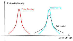
Pictorially, our result is summarized in Figure 1. We point out that the neural network training we consider is in the feature learning regime, where the weight parameters can go far away from their initialization. This is fundamentally different from the popular neural tangent kernel regime, where the neural networks essentially behave similar to its linearization.
1.1 Related Works
The Lottery Ticket Hypothesis and Sparse Training. The discovery of the lottery ticket hypothesis (Frankle and Carbin, 2018) has inspired further investigation and applications. One line of research has focused on developing computationally efficient methods to enable sparse training: the static sparse training methods are aiming at identifying a sparse mask at the initialization stage based on different criterion such as SNIP (loss-based) (Lee et al., 2018), GraSP (gradient-based) (Wang et al., 2019), SynFlow (synaptic strength-based) (Tanaka et al., 2020), neural tangent kernel based method (Liu and Zenke, 2020) and one-shot pruning (Chen et al., 2021a). Random pruning has also been considered in static sparse training such as uniform pruning (Mariet and Sra, 2015; He et al., 2017; Gale et al., 2019; Suau et al., 2018), non-uniform pruning (Mocanu et al., 2016), expander-graph-related techniques (Prabhu et al., 2018; Kepner and Robinett, 2019) Erdös-Rényi (Mocanu et al., 2018) and Erdös-Rényi-Kernel (Evci et al., 2020). On the other hand, dynamic sparse training allows the sparse mask to be updated (Mocanu et al., 2018; Mostafa and Wang, 2019; Evci et al., 2020; Jayakumar et al., 2020; Liu et al., 2021c, d, a; Peste et al., 2021). The sparsity pattern can also be learned by using sparsity-inducing regularizer (Yang et al., 2020). Recently, He et al. (2022) discovered that pruning can exhibit a double descent phenomenon when the data-set labels are corrupted.
Another line of research has focused on studying pruning the neural networks at its random initialization to achieve good performance (Zhou et al., 2019; Ramanujan et al., 2020). In particular, Ramanujan et al. (2020) showed that it is possible to prune a randomly initialized wide ResNet-50 to match the performance of a ResNet-34 trained on ImageNet. This phenomenon is named the strong lottery ticket hypothesis. Later, Malach et al. (2020) proved that under certain assumption on the initialization distribution, a target network of width and depth can be approximated by pruning a randomly initialized network that is of a polynomial factor (in ) wider and twice deeper even without any further training. However finding such a network is computationally hard, which can be shown by reducing the pruning problem to optimizing a neural network. Later, Pensia et al. (2020) improved the widening factor to being logarithmic and Sreenivasan et al. (2021) proved that with a polylogarithmic widening factor, such a result holds even if the network weight is binary. A follow-up work shows that it is possible to find a subnetwork achieving good performance at the initialization and then fine-tune (Sreenivasan et al., 2022). Our work, on the other hand, analyzes the gradient descent dynamics of a pruned neural network and its generalization after training.
Analyses of Training Neural Networks by Gradient Descent. A series of work (Allen-Zhu et al., 2019; Du et al., 2019; Lee et al., 2019; Zou et al., 2020; Zou and Gu, 2019; Ji and Telgarsky, 2019; Chen et al., 2020b; Song and Yang, 2019; Oymak and Soltanolkotabi, 2020) has proved that if a deep neural network is wide enough, then (stochastic) gradient descent provably can drive the training loss toward zero in a fast rate based on neural tangent kernel (NTK) (Jacot et al., 2018). Further, under certain assumption on the data, the learned network is able to generalize (Cao and Gu, 2019; Arora et al., 2019). However, as it is pointed out by Chizat et al. (2019), in the NTK regime, the gradient descent dynamics of the neural network essentially behaves similarly to its linearization and the learned weight is not far away from the initialization, which prohibits the network from performing any useful feature learning. In order to go beyond NTK regime, one line of research has focused on the mean field limit (Song et al., 2018; Chizat and Bach, 2018; Rotskoff and Vanden-Eijnden, 2018; Wei et al., 2019; Chen et al., 2020a; Sirignano and Spiliopoulos, 2020; Fang et al., 2021). Recently, people have started to study the neural network training dynamics in the feature learning regime where data from different class is defined by a set of class-related signals which are low rank (Allen-Zhu and Li, 2020, 2022; Cao et al., 2022; Shi et al., 2021; Telgarsky, 2022). However, all previous works did not consider the effect of pruning. Our work also focuses on the aforementioned feature learning regime, but for the first time characterizes the impact of pruning on the generalization performance of neural networks.
A prior work that is related to ours is (Zhang et al., 2021) which assumes the underlying data is generated by a sparse network and some variant of the true mask is known before training. They analyze training a sparse neural network and show that the sparse network can enjoy both faster convergence and smaller sample complexity. Our work also analyzes training a sparse neural network using gradient descent. However, different from their work, we don’t assume any information related to sparsity of the data is known before training and we prune the neural network simply by random pruning.
2 Preliminaries and Problem Formulation
In this section, we introduce our notation, data generation process, neural network architecture and the optimization algorithm.
Notations. We use lower case letters to denote scalars and boldface letters and symbols (e.g. ) to denote vectors and matrices. We use to denote element-wise product. For an integer , we use to denote the set of integers . We use to denote that there exists a constant such that respectively. We use and to hide polylogarithmic factor in these notations. Finally, we use if for some positive constant , and if .
2.1 Settings
Definition 2.1 (Data distribution of classes).
Consider we are given the set of signal vectors , where denotes the strength of the signal, and denotes the -th standard basis vector with its -th entry being 1 and all other coordinates being 0. Each data point with and is generated from the following distribution :
-
1.
The label is generated from a uniform distribution over .
-
2.
A noise vector is generated from the Gaussian distribution .
-
3.
With probability , assign ; with probability , assign where .
The sparse signal model is motivated by the empirical observation that during the process of training neural networks, the output of each layer of ReLU is usually sparse instead of dense. This is partially due to the fact that in practice the bias term in the linear layer is used (Song et al., 2021). For samples from different classes, usually a different set of neurons fire. Our study can be seen as a formal analysis on pruning the second last layer of a deep neural network in the layer-peeled model as in Zhu et al. (2021); Zhou et al. (2022). We also point out that our assumption on the sparsity of the signal is necessary for our analysis. If we don’t have this sparsity assumption and only make assumption on the norm of the signal, then in the extreme case, the signal is uniformly distributed across all coordinate and the effect of pruning to the signal and the noise will be essentially the same: their norm will both be reduced by a factor of .
Network architecture and random pruning. We consider a two-layer convolutional neural network model with polynomial ReLU activation , where we focus on the case when 111We point out that as many previous works (Allen-Zhu and Li, 2020; Zou et al., 2021; Cao et al., 2022), polynomial ReLU activation can help us simplify the analysis of gradient descent, because polynomial ReLU activation can give a much larger separation of signal and noise (thus, cleaner analysis) than ReLU. Our analysis can be generalized to ReLU activation by using the arguments in (Allen-Zhu and Li, 2022). The network is pruned at the initialization by mask where each entry in the mask is generated i.i.d. from . Let denotes the -th row of . Given the data , the output of the neural network can be written as where the -th output is given by
The mask is only sampled once at the initialization and remains fixed through the entire training process. From now on, we use tilde over a symbol to denote its masked version, e.g., and .
Since with probability , some neurons will not receive the corresponding signal at all and will only learn noise. Therefore, for each class , we split the neurons into two sets based on whether it receives its corresponding signal or not:
Gradient descent algorithm. We consider the network is trained by cross-entropy loss with softmax. We denote by and the cross-entropy loss can be written as . The convolutional neural network is trained by minimizing the empirical cross-entropy loss given by
where is the training data set. Similarly, we define the generalization loss as
The model weights are initialized from a i.i.d. Gaussian . The gradient of the cross-entropy loss is given by . Since
we can write the full-batch gradient descent update of the weights as
for and , where .
Condition 2.2.
We consider the parameter regime described as follows: (1) Number of classes . (2) Total number of training samples . (3) Dimension for some sufficiently large constant . (4) Relationship between signal strength and noise strength: . (5) The number of neurons in the network . (6) Initialization variance: . (7) Learning rate: . (8) Target training loss: .
Conditions (1) and (2) ensure that there are enough samples in each class with high probability. Condition (3) ensures that our setting is in high-dimensional regime. Condition (4) ensures that the full model can be trained to exhibit good generalization. Condition (5), (6) and (7) ensures that the neural network is sufficiently overparameterized and can be optimized efficiently by gradient descent. Condition (7) and (8) further ensures that training time is polynomial in . We further discuss the practical consideration of and to justify their condition in Remark D.9.
3 Mild Pruning
3.1 Main result
The first main result shows that there exists a threshold on the pruning fraction such that pruning helps the neural network’s generalization.
Theorem 3.1 (Main Theorem for Mild Pruning, Informal).
Under Condition 2.2, if for some constant , then with probability at least over the randomness in the data, network initialization and pruning, there exists such that
-
1.
The training loss is below : .
-
2.
The generalization loss can be bounded by .
Theorem 3.1 indicates that there exists a threshold in the order of such that if is above this threshold (i.e., the fraction of the pruned weights is small), gradient descent is able to drive the training loss towards zero (as item 1 claims) and the overparameterized network achieves good testing performance (as item 2 claims). In the next subsection, we explain why pruning can help generalization via an outline of our proof, and we defer all the detailed proofs in Appendix D.
3.2 Proof Outline
Our proof contains the establishment of the following two properties:
-
•
First we show that after mild pruning the network is still able to learn the signal, and the magnitude of the signal in the feature is preserved.
-
•
Then we show that given a new sample, pruning reduces the noise effect in the feature which leads to the improvement of generalization.
We first show the above properties for three stages of gradient descent: initialization, feature growing phase, and converging phase, and then establish the generalization property.
Initialization. First of all, readers might wonder why pruning can even preserve signal at all. Intuitively, a network will achieve good performance if its weights are highly correlated with the signal (i.e., their inner product is large). Two intuitive but misleading heuristics are given by the following:
-
•
Consider a fixed neuron weight. At the random initialization, in expectation, the signal correlation with the weights is given by and the noise correlation with the weights is given by by Jensen’s inequality. Based on this argument, taking a sum over all the neurons, pruning will hurt weight-signal correlation more than weight-noise correlation.
-
•
Since we are pruning with , a given neuron will not receive signal at all with probability . Thus, there is roughly fraction of the neurons receiving the signal and the rest fraction will be purely learning from noise. Even though for every neuron, roughly portion of mass from the noise is reduced, at the same time, pruning also creates fraction of neurons which do not receive signals at all and will purely output noise after training. Summing up the contributions from every neuron, the signal strength is reduced by a factor of while the noise strength is reduced by a factor of . We again reach the conclusion of pruning under any rate will hurt the signal more than noise.
The above analysis shows that under any pruning rate, it seems pruning can only hurt the signal more than noise at the initialization. Such analysis would be indicative if the network training is under the neural tangent kernel regime, where the weight of each neuron does not travel far from its initialization so that the above analysis can still hold approximately after training. However, when the neural network training is in the feature learning regime, this average type analysis becomes misleading. Namely, in such a regime, the weights with large correlation with the signal at the initialization will quickly evolve into singleton neurons and those weights with small correlation will remain small. In our proof, we focus on the featuring learning regime, and analyze how the network weights change and what are the effect of pruning during various stages of gradient descent.
We now analyze the effect of pruning on weight-signal correlation and weight-noise correlation at the initialization. Our first lemma leverages the sparsity of our signal and shows that if the pruning is mild, then it will not hurt the maximum weight-signal correlation much at the initialization. On the other hand, the maximum weight-noise correlation is reduced by a factor of .
Lemma 3.2 (Initialization).
With probability at least , for all ,
Further, suppose , with probability , for all ,
Given this lemma, we now prove that there exists at least one neuron that is heavily aligned with the signal after training. Similarly to previous works (Allen-Zhu and Li, 2020; Zou et al., 2021; Cao et al., 2022), the analysis is divided into two phases: feature growing phase and converging phase.
Feature Growing Phase. In this phase, the gradient of the cross-entropy is large and the weight-signal correlation grows much more quickly than weight-noise correlation thanks to the polynomial ReLU. We show that the signal strength is relatively unaffected by pruning while the noise level is reduced by a factor of .
Lemma 3.3 (Feature Growing Phase, Informal).
Under Condition 2.2, there exists time such that
-
1.
The max weight-signal correlation is large: for .
-
2.
The weight-noise and cross-class weight-signal correlations are small: if , then and .
Converging Phase. We show that gradient descent can drive the training loss toward zero while the signal in the feature is still large. An important intermediate step in our argument is the development of the following gradient upper bound for multi-class cross-entropy loss which introduces an extra factor of in the gradient upper bound.
Lemma 3.4 (Gradient Upper Bound, Informal).
Under Condition 2.2, we have
Proof Sketch.
To prove this upper bound, note that for a given input , should make major contribution to . Further note that . Now, apply the property that is small for (which we prove in the appendix), the numerator will contribute a factor of . To bound the rest, we utilize the special property of multi-class cross-entropy loss: . However, a naive application of this inequality will result in a factor of instead in our bound. The trick is to further use the fact that . ∎
Using the above gradient upper bound, we can show that the objective can be minimized.
Lemma 3.5 (Converging Phase, Informal).
Notice that the weight-noise correlation still remains reduced by a factor of after training. Lemma 3.5 proves the statement of the training loss in Theorem 3.1.
Generalization Analysis. Finally, we show that pruning can purify the feature by reducing the variance of the noise by a factor of when a new sample is given. The lemma below shows that the variance of weight-noise correlation for the trained weights is reduced by a factor of .
Lemma 3.6.
The neural network weight after training satisfies that
Using this lemma, we can show that pruning yields better generalization bound (i.e., the bound on the generalization loss) claimed in Theorem 3.1.
4 Over Pruning
Our second result shows that there exists a relatively large pruning fraction (i.e., small ) such that the learned model yields poor generalization, although gradient descent is still able to drive the training error toward zero. The full proof is defered to Appendix E.
Theorem 4.1 (Main Theorem for Over Pruning, Informal).
Under Condition 2.2 if , then with probability at least over the randomness in the data, network initialization and pruning, there exists such that
-
1.
The training loss is below : .
-
2.
The generalization loss is large: .
Remark 4.2.
The above theorem indicates that in the over-pruning case, the training loss can still go to zero. However, the generalization loss of our neural network behaves no much better than random guessing, because given any sample, random guessing will assign each class with probability , which yields a generalization loss of . The readers might wonder why the condition for this to happen is instead of . Indeed, the generalization will still be bad if is too small. However, now the neural network is not only unable to learn the signal but also cannot efficiently memorize the noise via gradient descent.
Proof Outline.
Now we analyze the over-pruning case. We first show that there is a good chance that the model will not receive any signal after pruning due to the sparse signal assumption and mild overparameterization of the neural network. Then, leveraging such a property, we bound the weight-signal and weight-noise properties for the feature growing and converging phases of gradient descent, as stated in the following two lemmas, respectively. Our result indicates that the training loss can still be driven toward zero by letting the neural network memorize the noise, the proof of which further exploits the fact that high dimensional Gaussian noise are nearly orthogonal.
Lemma 4.3 (Feature Growing Phase, Informal).
Under Condition 2.2, there exists such that
-
•
Some weights has large correlation with noise: for all .
-
•
The cross-class weight-noise and weight-signal correlations are small: if , then and .
Lemma 4.4 (Converging Phase, Informal).
Under Condition 2.2, there exists a time such that , the results from phase 1 still holds (up to constant factors) and .
Finally, since the above lemmas show that the network is purely memorizing the noise, we further show that such a network yields poor generalization performance as stated in Theorem 4.1. ∎
5 Experiments
5.1 Simulations to Verify Our Results
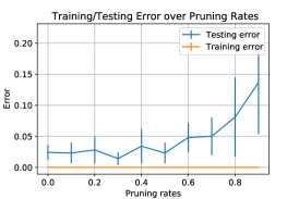
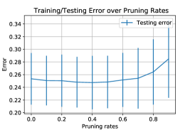
In this section, we conduct simulations to verify our results. We conduct our experiment using binary classification task and show that our result holds for ReLU networks. Our experiment settings are the follows: we choose input to be and , where is sampled from a Gaussian distribution. The class labels are . We use 100 training examples and 100 testing examples. The network has width and is initialized with random Gaussian distribution with variance 0.01. Then, fraction of the weights are randomly pruned. We use the learning rate of 0.001 and train the network over 1000 iterations by gradient descent.
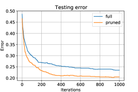
The observations are summarized as follows. In Figure 2a, when the noise level is , the pruned network usually can perform at the similar level with the full model when and noticably better when . When , the test error increases dramatically while the training accuracy still remains perfect. On the other hand, when the noise level becomes large (Figure 2b), the full model can no longer achieve good testing performance but mild pruning can improve the model’s generalization. Note that the training accuracy in this case is still perfect (omitted in the figure). We observe that in both settings when the model test error is large, the variance is also large. However, in Figure 2b, despite the large variance, the mean curve is already smooth. In particular, Figure 2c plots the testing error over the training iterations under pruning rate. This suggests that pruning can be beneficial even when the input noise is large.
5.2 On the Real World Dataset
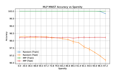
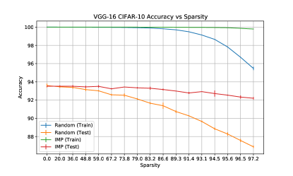
To further demonstrate the mild/over pruning phenomenon, we conduct experiments on MNIST (Deng, 2012) and CIFAR-10 (Krizhevsky et al., 2009) datasets. We consider neural network architectures including MLP with 2 hidden layers of width 1024, VGG, ResNets (He et al., 2016) and wide ResNet (Zagoruyko and Komodakis, 2016). In addition to random pruning, we also add iterative-magnitude-based pruning Frankle and Carbin (2018) into our experiments. Both pruning methods are prune-at-initialization methods. Our implementation is based on Chen et al. (2021c).
Under the real world setting, we do not expect our theorem to hold exactly. Instead, our theorem implies that (1) there exists a threshold such that the testing performance is no much worse than (or sometimes may slightly better than) its dense counter part; and (2) the training error decreases later than the testing error decreases. Our experiments on MLP (Figure 3a) and VGG-16 (Figure 3b) show that this is the case: for MLP the test accuracy is steady competitive to its dense counterpart when the sparsity is less than and for VGG-16. We further provide experiments on ResNet in the appendix for validation of our theoretical results.
6 Discussion and Future Direction
In this work, we provide theory on the generalization performance of pruned neural networks trained by gradient descent under different pruning rates. Our results characterize the effect of pruning under different pruning rates: in the mild pruning case, the signal in the feature is well-preserved and the noise level is reduced which leads to improvement in the trained network’s generalization; on the other hand, over pruning significantly destroys signal strength despite of reducing noise variance. One open problem on this topic still appears challenging. In this paper, we characterize two cases of pruning: in mild pruning the signal is preserved and in over pruning the signal is completely destroyed. However, the transition between these two cases is not well-understood. Further, it would be interesting to consider more general data distribution, and understand how pruning affects training multi-layer neural networks. We leave these interesting directions as future works.
References
- Allen-Zhu and Li (2020) Allen-Zhu, Z. and Li, Y. (2020). Towards understanding ensemble, knowledge distillation and self-distillation in deep learning. arXiv preprint arXiv:2012.09816 .
- Allen-Zhu and Li (2022) Allen-Zhu, Z. and Li, Y. (2022). Feature purification: How adversarial training performs robust deep learning. In 2021 IEEE 62nd Annual Symposium on Foundations of Computer Science (FOCS). IEEE.
- Allen-Zhu et al. (2019) Allen-Zhu, Z., Li, Y. and Song, Z. (2019). A convergence theory for deep learning via over-parameterization. In International Conference on Machine Learning. PMLR.
- Arora et al. (2019) Arora, S., Du, S., Hu, W., Li, Z. and Wang, R. (2019). Fine-grained analysis of optimization and generalization for overparameterized two-layer neural networks. In International Conference on Machine Learning. PMLR.
- Cao et al. (2022) Cao, Y., Chen, Z., Belkin, M. and Gu, Q. (2022). Benign overfitting in two-layer convolutional neural networks. arXiv preprint arXiv:2202.06526 .
- Cao and Gu (2019) Cao, Y. and Gu, Q. (2019). Generalization bounds of stochastic gradient descent for wide and deep neural networks. Advances in neural information processing systems 32.
- Chen et al. (2021a) Chen, T., Ji, B., Ding, T., Fang, B., Wang, G., Zhu, Z., Liang, L., Shi, Y., Yi, S. and Tu, X. (2021a). Only train once: A one-shot neural network training and pruning framework. Advances in Neural Information Processing Systems 34.
- Chen et al. (2021b) Chen, T., Zhang, Z., Balachandra, S., Ma, H., Wang, Z., Wang, Z. et al. (2021b). Sparsity winning twice: Better robust generalization from more efficient training. In International Conference on Learning Representations.
- Chen et al. (2021c) Chen, X., Cheng, Y., Wang, S., Gan, Z., Liu, J. and Wang, Z. (2021c). The elastic lottery ticket hypothesis. Github Repository, MIT License .
- Chen et al. (2020a) Chen, Z., Cao, Y., Gu, Q. and Zhang, T. (2020a). A generalized neural tangent kernel analysis for two-layer neural networks. Advances in Neural Information Processing Systems 33 13363–13373.
- Chen et al. (2020b) Chen, Z., Cao, Y., Zou, D. and Gu, Q. (2020b). How much over-parameterization is sufficient to learn deep relu networks? In International Conference on Learning Representations.
- Chizat and Bach (2018) Chizat, L. and Bach, F. (2018). On the global convergence of gradient descent for over-parameterized models using optimal transport. Advances in neural information processing systems 31.
- Chizat et al. (2019) Chizat, L., Oyallon, E. and Bach, F. (2019). On lazy training in differentiable programming. Advances in Neural Information Processing Systems 32.
- Deng (2012) Deng, L. (2012). The mnist database of handwritten digit images for machine learning research [best of the web]. IEEE signal processing magazine 29 141–142.
- Ding et al. (2021) Ding, S., Chen, T. and Wang, Z. (2021). Audio lottery: Speech recognition made ultra-lightweight, noise-robust, and transferable. In International Conference on Learning Representations.
- Du et al. (2019) Du, S., Lee, J., Li, H., Wang, L. and Zhai, X. (2019). Gradient descent finds global minima of deep neural networks. In International conference on machine learning. PMLR.
- Evci et al. (2020) Evci, U., Gale, T., Menick, J., Castro, P. S. and Elsen, E. (2020). Rigging the lottery: Making all tickets winners. In International Conference on Machine Learning. PMLR.
- Fang et al. (2021) Fang, C., Lee, J., Yang, P. and Zhang, T. (2021). Modeling from features: a mean-field framework for over-parameterized deep neural networks. In Conference on learning theory. PMLR.
- Frankle and Carbin (2018) Frankle, J. and Carbin, M. (2018). The lottery ticket hypothesis: Finding sparse, trainable neural networks. In International Conference on Learning Representations.
- Frankle et al. (2020) Frankle, J., Dziugaite, G. K., Roy, D. and Carbin, M. (2020). Pruning neural networks at initialization: Why are we missing the mark? In International Conference on Learning Representations.
- Gale et al. (2019) Gale, T., Elsen, E. and Hooker, S. (2019). The state of sparsity in deep neural networks. arXiv preprint arXiv:1902.09574 .
- He et al. (2016) He, K., Zhang, X., Ren, S. and Sun, J. (2016). Deep residual learning for image recognition. In Proceedings of the IEEE conference on computer vision and pattern recognition.
- He et al. (2017) He, Y., Zhang, X. and Sun, J. (2017). Channel pruning for accelerating very deep neural networks. In Proceedings of the IEEE international conference on computer vision.
- He et al. (2022) He, Z., Xie, Z., Zhu, Q. and Qin, Z. (2022). Sparse double descent: Where network pruning aggravates overfitting. In International Conference on Machine Learning. PMLR.
- Jacot et al. (2018) Jacot, A., Gabriel, F. and Hongler, C. (2018). Neural tangent kernel: Convergence and generalization in neural networks. Advances in neural information processing systems 31.
- Jayakumar et al. (2020) Jayakumar, S., Pascanu, R., Rae, J., Osindero, S. and Elsen, E. (2020). Top-kast: Top-k always sparse training. Advances in Neural Information Processing Systems 33 20744–20754.
- Ji and Telgarsky (2019) Ji, Z. and Telgarsky, M. (2019). Polylogarithmic width suffices for gradient descent to achieve arbitrarily small test error with shallow relu networks. In International Conference on Learning Representations.
- Kepner and Robinett (2019) Kepner, J. and Robinett, R. (2019). Radix-net: Structured sparse matrices for deep neural networks. In 2019 IEEE International Parallel and Distributed Processing Symposium Workshops (IPDPSW). IEEE.
- Krizhevsky et al. (2009) Krizhevsky, A., Hinton, G. et al. (2009). Learning multiple layers of features from tiny images .
- LeCun et al. (1989) LeCun, Y., Denker, J. and Solla, S. (1989). Optimal brain damage. Advances in neural information processing systems 2.
- Lee et al. (2019) Lee, J., Xiao, L., Schoenholz, S., Bahri, Y., Novak, R., Sohl-Dickstein, J. and Pennington, J. (2019). Wide neural networks of any depth evolve as linear models under gradient descent. Advances in neural information processing systems 32.
- Lee et al. (2018) Lee, N., Ajanthan, T. and Torr, P. (2018). Snip: Single-shot network pruning based on connection sensitivity. In International Conference on Learning Representations.
- Liu et al. (2021a) Liu, S., Chen, T., Chen, X., Atashgahi, Z., Yin, L., Kou, H., Shen, L., Pechenizkiy, M., Wang, Z. and Mocanu, D. C. (2021a). Sparse training via boosting pruning plasticity with neuroregeneration. Advances in Neural Information Processing Systems 34.
- Liu et al. (2021b) Liu, S., Chen, T., Chen, X., Shen, L., Mocanu, D. C., Wang, Z. and Pechenizkiy, M. (2021b). The unreasonable effectiveness of random pruning: Return of the most naive baseline for sparse training. In International Conference on Learning Representations.
- Liu et al. (2021c) Liu, S., Mocanu, D. C., Matavalam, A. R. R., Pei, Y. and Pechenizkiy, M. (2021c). Sparse evolutionary deep learning with over one million artificial neurons on commodity hardware. Neural Computing and Applications 33 2589–2604.
- Liu et al. (2021d) Liu, S., Yin, L., Mocanu, D. C. and Pechenizkiy, M. (2021d). Do we actually need dense over-parameterization? in-time over-parameterization in sparse training. In International Conference on Machine Learning. PMLR.
- Liu and Zenke (2020) Liu, T. and Zenke, F. (2020). Finding trainable sparse networks through neural tangent transfer. In International Conference on Machine Learning. PMLR.
- Luo and Wu (2017) Luo, J.-H. and Wu, J. (2017). An entropy-based pruning method for cnn compression. arXiv preprint arXiv:1706.05791 .
- Malach et al. (2020) Malach, E., Yehudai, G., Shalev-Schwartz, S. and Shamir, O. (2020). Proving the lottery ticket hypothesis: Pruning is all you need. In International Conference on Machine Learning. PMLR.
- Mariet and Sra (2015) Mariet, Z. and Sra, S. (2015). Diversity networks: Neural network compression using determinantal point processes. arXiv preprint arXiv:1511.05077 .
- Mocanu et al. (2016) Mocanu, D. C., Mocanu, E., Nguyen, P. H., Gibescu, M. and Liotta, A. (2016). A topological insight into restricted boltzmann machines. Machine Learning 104 243–270.
- Mocanu et al. (2018) Mocanu, D. C., Mocanu, E., Stone, P., Nguyen, P. H., Gibescu, M. and Liotta, A. (2018). Scalable training of artificial neural networks with adaptive sparse connectivity inspired by network science. Nature communications 9 1–12.
- Molchanov et al. (2019) Molchanov, P., Tyree, S., Karras, T., Aila, T. and Kautz, J. (2019). Pruning convolutional neural networks for resource efficient inference. In 5th International Conference on Learning Representations, ICLR 2017-Conference Track Proceedings.
- Mostafa and Wang (2019) Mostafa, H. and Wang, X. (2019). Parameter efficient training of deep convolutional neural networks by dynamic sparse reparameterization. In International Conference on Machine Learning. PMLR.
- Oymak and Soltanolkotabi (2020) Oymak, S. and Soltanolkotabi, M. (2020). Toward moderate overparameterization: Global convergence guarantees for training shallow neural networks. IEEE Journal on Selected Areas in Information Theory 1 84–105.
- Pensia et al. (2020) Pensia, A., Rajput, S., Nagle, A., Vishwakarma, H. and Papailiopoulos, D. (2020). Optimal lottery tickets via subset sum: Logarithmic over-parameterization is sufficient. Advances in Neural Information Processing Systems 33 2599–2610.
- Peste et al. (2021) Peste, A., Iofinova, E., Vladu, A. and Alistarh, D. (2021). Ac/dc: Alternating compressed/decompressed training of deep neural networks. Advances in Neural Information Processing Systems 34.
- Prabhu et al. (2018) Prabhu, A., Varma, G. and Namboodiri, A. (2018). Deep expander networks: Efficient deep networks from graph theory. In Proceedings of the European Conference on Computer Vision (ECCV).
- Ramanujan et al. (2020) Ramanujan, V., Wortsman, M., Kembhavi, A., Farhadi, A. and Rastegari, M. (2020). What’s hidden in a randomly weighted neural network? In Proceedings of the IEEE CVF Conference on Computer Vision and Pattern Recognition.
- Rotskoff and Vanden-Eijnden (2018) Rotskoff, G. M. and Vanden-Eijnden, E. (2018). Neural networks as interacting particle systems: Asymptotic convexity of the loss landscape and universal scaling of the approximation error. stat 1050 22.
- Shi et al. (2021) Shi, Z., Wei, J. and Liang, Y. (2021). A theoretical analysis on feature learning in neural networks: Emergence from inputs and advantage over fixed features. In International Conference on Learning Representations.
- Sirignano and Spiliopoulos (2020) Sirignano, J. and Spiliopoulos, K. (2020). Mean field analysis of neural networks: A law of large numbers. SIAM Journal on Applied Mathematics 80 725–752.
- Song et al. (2018) Song, M., Montanari, A. and Nguyen, P. (2018). A mean field view of the landscape of two-layers neural networks. Proceedings of the National Academy of Sciences 115 E7665–E7671.
- Song et al. (2021) Song, Z., Yang, S. and Zhang, R. (2021). Does preprocessing help training over-parameterized neural networks? Advances in Neural Information Processing Systems 34.
- Song and Yang (2019) Song, Z. and Yang, X. (2019). Quadratic suffices for over-parametrization via matrix chernoff bound. arXiv preprint arXiv:1906.03593 .
- Sreenivasan et al. (2021) Sreenivasan, K., Rajput, S., Sohn, J.-y. and Papailiopoulos, D. (2021). Finding everything within random binary networks. arXiv preprint arXiv:2110.08996 .
- Sreenivasan et al. (2022) Sreenivasan, K., Sohn, J.-y., Yang, L., Grinde, M., Nagle, A., Wang, H., Lee, K. and Papailiopoulos, D. (2022). Rare gems: Finding lottery tickets at initialization. arXiv preprint arXiv:2202.12002 .
- Su et al. (2020) Su, J., Chen, Y., Cai, T., Wu, T., Gao, R., Wang, L. and Lee, J. D. (2020). Sanity-checking pruning methods: Random tickets can win the jackpot. Advances in Neural Information Processing Systems 33 20390–20401.
- Suau et al. (2018) Suau, X., Zappella, L. and Apostoloff, N. (2018). Network compression using correlation analysis of layer responses .
- Tanaka et al. (2020) Tanaka, H., Kunin, D., Yamins, D. L. and Ganguli, S. (2020). Pruning neural networks without any data by iteratively conserving synaptic flow. Advances in Neural Information Processing Systems 33 6377–6389.
- Telgarsky (2022) Telgarsky, M. (2022). Feature selection with gradient descent on two-layer networks in low-rotation regimes. arXiv preprint arXiv:2208.02789 .
- Wang et al. (2019) Wang, C., Zhang, G. and Grosse, R. (2019). Picking winning tickets before training by preserving gradient flow. In International Conference on Learning Representations.
- Wei et al. (2019) Wei, C., Lee, J. D., Liu, Q. and Ma, T. (2019). Regularization matters: Generalization and optimization of neural nets vs their induced kernel. Advances in Neural Information Processing Systems 32.
- Yang et al. (2020) Yang, H., Wen, W. and Li, H. (2020). Deephoyer: Learning sparser neural network with differentiable scale-invariant sparsity measures. In International Conference on Learning Representations.
- Yang et al. (2021) Yang, Q., Mao, J., Wang, Z. and Hai, H. L. (2021). Dynamic regularization on activation sparsity for neural network efficiency improvement. ACM Journal on Emerging Technologies in Computing Systems (JETC) 17 1–16.
- Ye et al. (2020) Ye, M., Gong, C., Nie, L., Zhou, D., Klivans, A. and Liu, Q. (2020). Good subnetworks provably exist: Pruning via greedy forward selection. In International Conference on Machine Learning. PMLR.
- Zagoruyko and Komodakis (2016) Zagoruyko, S. and Komodakis, N. (2016). Wide residual networks. In British Machine Vision Conference 2016. British Machine Vision Association.
- Zhang et al. (2021) Zhang, S., Wang, M., Liu, S., Chen, P.-Y. and Xiong, J. (2021). Why lottery ticket wins? a theoretical perspective of sample complexity on sparse neural networks. Advances in Neural Information Processing Systems 34 2707–2720.
- Zhou et al. (2019) Zhou, H., Lan, J., Liu, R. and Yosinski, J. (2019). Deconstructing lottery tickets: Zeros, signs, and the supermask. Advances in neural information processing systems 32.
- Zhou et al. (2022) Zhou, J., Li, X., Ding, T., You, C., Qu, Q. and Zhu, Z. (2022). On the optimization landscape of neural collapse under mse loss: Global optimality with unconstrained features. arXiv preprint arXiv:2203.01238 .
- Zhu et al. (2021) Zhu, Z., Ding, T., Zhou, J., Li, X., You, C., Sulam, J. and Qu, Q. (2021). A geometric analysis of neural collapse with unconstrained features. Advances in Neural Information Processing Systems 34.
- Zou et al. (2021) Zou, D., Cao, Y., Li, Y. and Gu, Q. (2021). Understanding the generalization of adam in learning neural networks with proper regularization. arXiv preprint arXiv:2108.11371 .
- Zou et al. (2020) Zou, D., Cao, Y., Zhou, D. and Gu, Q. (2020). Gradient descent optimizes over-parameterized deep relu networks. Machine Learning 109 467–492.
- Zou and Gu (2019) Zou, D. and Gu, Q. (2019). An improved analysis of training over-parameterized deep neural networks. Advances in neural information processing systems 32.
Appendix A Experiment Details
The experiments of MLP, VGG and ResNet-32 are run on NVIDIA A5000 and ResNet-50 and ResNet-20-128 is run on 4 NIVIDIA V100s. We list the hyperparameters we used in training. All of our models are trained with SGD and the detailed settings are summarized below.
| Model | Data | Epoch | Batch Size | LR | Momentum | LR Decay, Epoch | Weight Decay |
| LeNet | MNIST | 120 | 128 | 0.1 | 0 | 0 | 0 |
| VGG | CIFAR-10 | 160 | 128 | 0.1 | 0.9 | 0.1 [80, 120] | 0.0001 |
| ResNets | CIFAR-10 | 160 | 128 | 0.1 | 0.9 | 0.1 [80, 120] | 0.0001 |
Appendix B Further Experiment Results
We plot the experiment result of ResNet-20-128 in Figure 4. This figure further verifies our results that there exists pruning rate threshold such that the testing performance of the pruned network is on par with the testing performance of the dense model while the training accuracy remains perfect.

Appendix C Preliminary for Analysis
In this section, we introduce the following signal-noise decomposition of each neuron weight from Cao et al. (2022), and some useful properties for the terms in such a decomposition, which are useful in our analysis.
Definition C.1 (signal-noise decomposition).
For each neuron weight , there exist coefficients such that
where .
It is straightforward to see the following:
where are increasing sequences and are decreasing sequences, because when , and when . By Lemma D.4, we have , and hence the set of vectors is linearly independent with probability measure 1 over the Gaussian distribution for each . Therefore the decomposition is unique.
Appendix D Proof of Theorem 3.1
We first formally restate Theorem 3.1.
Theorem D.1 (Formal Restatement of Theorem 3.1).
Under Condition 2.2, choose initialization variance and learning rate . For , if for some sufficiently large constant , then with probability at least over the randomness in the data, network initialization and pruning, there exists such that the following holds:
-
1.
The training loss is below : .
-
2.
The weights of the CNN highly correlate with its corresponding class signal: for all .
-
3.
The weights of the CNN doesn’t have high correlation with the signal from different classes: .
-
4.
None of the weights is highly correlated with the noise: .
Moreover, the testing loss is upper-bounded by
The proof of Theorem 3.1 consists of the analysis of the pruning on the signal and noise for three stages of gradient descent: initialization, feature growing phase, and converging phase, and the establishment of the generalization property. We present these analysis in detail in the following subsections. A special note is that the constant showing up in the following proof of each subsequent Lemmas is defined locally instead of globally, which means the constant within each Lemma is the same but may be different across different Lemma.
D.1 Initialization
We analyze the effect of pruning on weight-signal correlation and weight-noise correlation at the initialization. We first present a few supporting lemmas, and finally provide our main result of Lemma D.7, which shows that if the pruning is mild, then it will not hurt the max weight-signal correlation much at the initialization. On the other hand, the max weight-noise correlation is reduced by a factor of .
Lemma D.2.
Assume . Then, with probability at least ,
Proof.
By Hoeffding’s inequality, with probability at least , for a fixed , we have
Therefore, as long as , we have
Taking a union bound over and making yield the result. ∎
Lemma D.3.
Assume and . Then, with probability , for all , we have , which implies that for all .
Proof.
When , by multiplicative Chernoff’s bound, for a given , we have
Take a union bound over , we have
∎
Lemma D.4.
Assume . Then with probability at least , for all , , .
Proof.
By multiplicative Chernoff’s bound, we have for a given
Take a union bound over , we have
where the last inequality follows from our choices of . ∎
Lemma D.5.
Suppose , and . With probability at least , we have
for all and .
Proof.
From Lemma D.4, we have with probability at least ,
For a set of Gaussian random variable , by Bernstein’s inequality, with probability at least , we have
Thus, by a union bound over , with probability at least , we have
For , again by Bernstein’s bound, we have with probability at least ,
for all . Plugging in gives the result. The proof for is similar. ∎
Lemma D.6.
Suppose we have independent Gaussian random variables . Then with probability ,
Proof.
By the standard tail bound of Gaussian random variable, we have for every ,
We want to pick a such that
∎
Lemma D.7 (Formal Restatement of Lemma 3.2).
With probability at least , for all ,
Further, suppose . Then with probability , for all ,
Proof.
We first give a proof for the second inequality. From Lemma D.3, we know that . The upper bound can be obtained by taking a union bound over . To prove the lower bound, applying Lemma D.6, with probability at least , we have for a given
Now, notice that we can control the constant in (by controlling the constant in the lower bound of ) such that . Thus, taking a union bound over and setting yield the result.
The proof of the first inequality is similar. ∎
D.2 Supporting Properties for Entire Training Process
This subsection establishes a few properties (summarized in Proposition D.10) that will be used in the analysis of feature growing phase and converging phase of gradient descent presented in the next two subsections. Define . Denote . We need the following bound holds for our subsequent analysis.
| (D.1) |
Remark D.8.
To see why Equation D.1 can hold under 2.2, we convert everything in terms of . First recall from 2.2 that and . In both mild pruning and over pruning we require . Since , if we assume for a moment (which we are going to justify in the next paragraph), then . Then if we set to be large enough, we have . Finally for the quantity , by Lemma 3.2, our assumption of in 2.2 and our choice of in Theorem 3.1 (or Theorem D.1), we can easily see that this quantity can also be made smaller than 1.
Now, to justify that , we only need to justify that all the quantities depend on is polynomial in . First of all, based on 2.2, and further implies . Since Theorem 3.1 only requires , this implies . Hence . Together with our assumption that (which implies ), we have justified that all terms involved in are at most of order . Hence .
Remark D.9.
Here we make remark on our assumption on and in 2.2.
For our assumption on , since the cross-entropy loss is (1) not strongly-convex and (2) achieves its infimum at infinity. In practice, the cross-entropy loss is minimized to a constant level, say 0.001. We make this assumption to avoid the pathological case where is exponentially small in (say ) which is unrealistic. Thus, for realistic setting, we assume or .
To deal with , the only restriction we have is in Theorem 3.1 and Theorem 4.1. However, in practice, we don’t use a learning rate that is exponentially small, say . Thus, like dealing with , we assume or .
We make the above assumption to simplify analysis when analyzing the magnitude of for given sample .
Proposition D.10.
Under 2.2, during the training time , we have
-
1.
,
-
2.
.
-
3.
.
Notice that the lower bound has absolute value smaller than the upper bound.
Proof of Proposition D.10.
We use induction to prove Proposition D.10.
Induction Hypothesis:
Suppose Proposition D.10 holds for all .
We next show that this also holds for via the following a few lemmas.
Lemma D.11.
Under 2.2, for , there exists a constant such that
Proof.
From Lemma D.5, there exists a constant such that with probability at least ,
Using the signal-noise decomposition and assuming , we have
where the second last inequality is by Lemma D.5 and the last inequality is by induction hypothesis.
To prove the second equality, for ,
where the last inequality is by and . The proof for the case of is similar. ∎
Lemma D.12 (Off-diagonal Correlation Upper Bound).
Under 2.2, for , , we have that
Proof.
If , then and we have that
Further, we can obtain
Then, we have the following bound:
where the first inequality is by Equation D.1. ∎
Lemma D.13 (Diagonal Correlation Upper Bound).
Proof.
Lemma D.14.
Under 2.2, for , we have that
-
1.
;
-
2.
.
Proof.
When , we have . We only need to consider the case of . When , by Lemma D.11 we have
Thus,
When , we have
where the last inequality is by setting and is the constant such that for all in Lemma D.5.
For , the proof is similar. Consider . When , by Lemma D.11, we have
Hence,
When , we have
where the first inequality follows from the fact that there are samples such that , and the last inequality follows from picking . ∎
Lemma D.15.
Under 2.2, for , we have .
Proof.
For or , .
We first bound . Let be the last time that . Then we have
We bound separately. We first bound as follows.
where the first inequality follows from Lemma D.13, the second inequality follows because and , and the last inequality follows because .
For , by Lemma D.11, we have that and .
Now we bound as follows
where the first inequality follows from Equation (D.2), the second inequality follows because , the fourth inequality follows by choosing , and the last inequality follows by choosing .
Plugging the bounds on finishes the proof for .
To prove , we pick and the rest of the proof is similar. ∎
Induction Ends
∎
D.3 Feature Growing Phase
In this subsection, we first present a supporting lemma, and then provide our main result of Lemma D.17, which shows that the signal strength is relatively unaffected by pruning while the noise level is reduced by a factor of .
During the feature growing phase of training, the output of for all . Therefore, and until reaches .
Lemma D.16.
Under the same assumption as Theorem D.1, for , the following results hold:
-
•
for all and .
-
•
for all and .
Proof.
Define . Then we have
where the second inequality follows by and applying the bounds from Lemma D.5, and the last inequality follows by choosing . Let be the constants for the upper bound to hold in the big O notation. For any , we use induction to show that
| (D.3) |
Suppose that Equation (D.3) holds for for . Then
where the last inequality follows by picking . Therefore, by induction, we have for all . ∎
Lemma D.17 (Formal Restatement of Lemma 3.3).
Under the same assumption as Theorem D.1, there exists time such that
-
1.
for .
-
2.
for all and .
-
3.
for all and .
Proof.
Consider a fixed class . Denote to be the last time for satisfying . Then for , and . Thus, by Lemma D.13, we obtain that . Thus, . For , we have
Let and . Note that by our choice of , we have . Since by Lemma D.7, . Then we have
Therefore, the sequence will exponentially grow and will reach within . Thus, .
Now we prove that under the same assumption as Theorem D.1, for , we have for all and .
We show that there exists a time such that for all , . Let .
Define . Since we assume , by Lemma D.16, we have .
where the first inequality follows because , the second inequality follows because there are samples from a given class and , and the last inequality follows because . Now, let be the constant such that the above holds with big O. Then, we use induction to show that for all . We proceed as follows.
where the last inequality follows by picking . ∎
D.4 Converging Phase
In this subsection, we show that gradient descent can drive the training loss toward zero while the signal in the feature is still large. An important intermediate step in our argument is the development of the following gradient upper bound for multi-class cross-entropy loss.
In this phase, we are going to show that
-
•
for all .
-
•
where .
-
•
where
Define as follows:
Lemma D.18.
Based on the result from the feature growing phase, .
Proof.
We first compute
where the first inequality follows from triangle inequality, the second inequality follows from Lemma D.17, and the last inequality follows from our choice of . On the other hand,
Thus, we obtain
∎
Lemma D.19 (Gradient Upper Bound).
Under 2.2, for , there exists constant such that
Proof.
We need to prove that . Assume . Then we obtain
where the first and second inequality follow from triangle inequality, the third inequality follows from Hölder’s inequality, and the last inequality follows from Lemma D.12. Similarly, on the other hand, if , then
Therefore,
and
where the inequality follows from Equation (D.2). Thus,
| (D.4) |
where the first inequality follows because , and the last inequality uses the fact that for all .
The gradient norm can be bounded by
where the first inequality uses triangle inequality, the second inequality follows because , the third inequality uses the bound (D.4), the fourth inequality uses Jensen’s inequality and the last inequality follows because . ∎
Lemma D.20.
For , we have for all ,
Proof of Lemma D.20.
The proof of this lemma depends on the next two lemmas.
Lemma D.21.
For and , we have .
Proof.
By Lemma D.17, we have
where the last inequality follows by picking . On the other hand,
| (D.5) |
where the first inequality follows from Lemma D.11 and the second inequality follows from Equation D.1 and Proposition D.10. Therefore,
where the last inequality follows because and by our choices of . ∎
Lemma D.22.
For and , we have .
Proof.
Lemma D.23.
Under the same assumption as Theorem D.1, we have
Proof.
To simplify our notation, we define .
Lemma D.24 (Formal Restatement of Lemma 3.5).
Under the same assumption as Theorem D.1, choose . Then for any time during this stage, we have for all , , and
Proof.
From Lemma D.17, we have and since is an increasing sequence over , we have for all . We have
Taking a telescopic sum from to yields
Combining Lemma D.18, we have
| (D.7) |
Define and and . Now we use induction to prove and . Suppose the result holds for time . Then
where the second inequality follows by and applying the bounds from Lemma D.5, and the last inequality follows by choosing . Unrolling the recursion by taking a sum from to we have
where (i) follows from induction hypothesis , (ii) follows from the property of cross-entropy loss with softmax , (iii) follows from Equation (D.7), (iv) follows from our choice of , and (v) follows because . Therefore, by induction holds for time .
D.5 Generalization Analysis
In this subsection, we show that pruning can purify the feature by reducing the variance of the noise by a factor of when a new sample is given.
Now the network has parameter
We have .
Lemma D.25 (Formal Restatement of Lemma 3.6).
With probability at least ,
Proof.
Since follows a Gaussian distribution with variance , we have
Applying a union bound over gives the result. ∎
Theorem D.26 (Formal Restatement of Generalization Part of Theorem 3.1).
Under the same assumptions as Theorem D.1, within iterations, we can find such that
-
•
.
-
•
.
Proof.
Let be the event that Lemma D.25 holds. Then, we can divide into two parts:
Since , for each class there must exist one training sample with such that by pigeonhole principle. This implies that . Conditioning on the event , by Lemma D.25, we have
Thus, we have . Next we bound the term .
| (D.8) |
where the first inequality follows because , the second and third inequalities follow from the property of log function, and the last inequality follows from our choice of . We further have
where the first inequality follows from Cauchy-Schwarz inequality, the second inequality follows from Equation (D.5), the third inequality follows from Lemma D.25, and the last inequality follows because .
∎
Appendix E Proof of Theorem 4.1
In this section, we show that there exists a relatively large pruning fraction (i.e., small ) such that while gradient descent is still able to drive the training error toward zero, the learned model yields poor generalization. We first provide a formal restatement of Theorem 4.1.
Theorem E.1 (Formal Restatement of Theorem 4.1).
Under Condition 2.2, choose initialization variance and learning rate . For , if , then with probability at least , there exists such that the following holds:
-
1.
The training loss is below : .
-
2.
The model weight doesn’t learn any of its corresponding signal at all: for all .
-
3.
The model weights is highly correlated with the noise: if .
Moreover, the testing loss is large:
The proof of Theorem 4.1 consists of the analysis of the over-pruning for three stages of gradient descent: initialization, feature growing phase, and converging phase, and the establishment of the generalization property. We present these analysis in detail in the following subsections.
E.1 Initialization
Lemma E.2.
When and , with probability , for all class we have .
Proof.
First, the probability that a given class receives no signal is . We use the inequality that
Then the probability that is given by
∎
E.2 Feature Growing Phase
E.3 Converging Phase
From the first stage we know that
Now we define as follows:
Lemma E.4.
Based on the result from feature growing phase, .
Proof.
We derive the following bound:
where the first inequality follows from triangle inequality, the second inequality follows from the expression of , and the third inequality follows from Lemma D.5 and the fact that if and only if . ∎
Lemma E.5.
For , we have
Lemma E.6.
For and , we have
Lemma E.7.
For and , we have
Proof.
Lemma E.8.
Under the same assumption as Theorem E.1, we have
Proof.
To simplify our notation, we define . The proof is exactly the same as the proof of Lemma D.23.
where the first inequality follows from the convexity of the cross-entropy loss with softmax, the second inequality follows from Lemma D.20, the third inequality follows because , and the last inequality follows from Lemma D.19 for some constant . ∎
Lemma E.9 (Formal Restatement of Lemma 4.4).
Under the same assumption as Theorem E.1, choose . Then for any time during this stage we have and
Proof.
E.4 Generalization Analysis
Theorem E.10 (Formal Restatement of the Generalization Part of Theorem 4.1).
Under the same assumption as Theorem E.1, within iterations, we can find such that , and .
Proof.
First of all, from Lemma E.9 we know there exists such that . Then, we can bound
Consider a new example . Taking a union bound over , with probability at least , we have
for all . Then,
where the last inequality follows because and . Thus, with probability at least ,
∎