DensePose From WiFi

Abstract.

Advances in computer vision and machine learning techniques have led to significant development in 2D and 3D human pose estimation from RGB cameras, LiDAR, and radars. However, human pose estimation from images is adversely affected by occlusion and lighting, which are common in many scenarios of interest. Radar and LiDAR technologies, on the other hand, need specialized hardware that is expensive and power-intensive. Furthermore, placing these sensors in non-public areas raises significant privacy concerns.

To address these limitations, recent research has explored the use of WiFi antennas (1D sensors) for body segmentation and key-point body detection. This paper further expands on the use of the WiFi signal in combination with deep learning architectures, commonly used in computer vision, to estimate dense human pose correspondence. We developed a deep neural network that maps the phase and amplitude of WiFi signals to UV coordinates within 24 human regions. The results of the study reveal that our model can estimate the dense pose of multiple subjects, with comparable performance to image-based approaches, by utilizing WiFi signals as the only input. This paves the way for low-cost, broadly accessible, and privacy-preserving algorithms for human sensing.

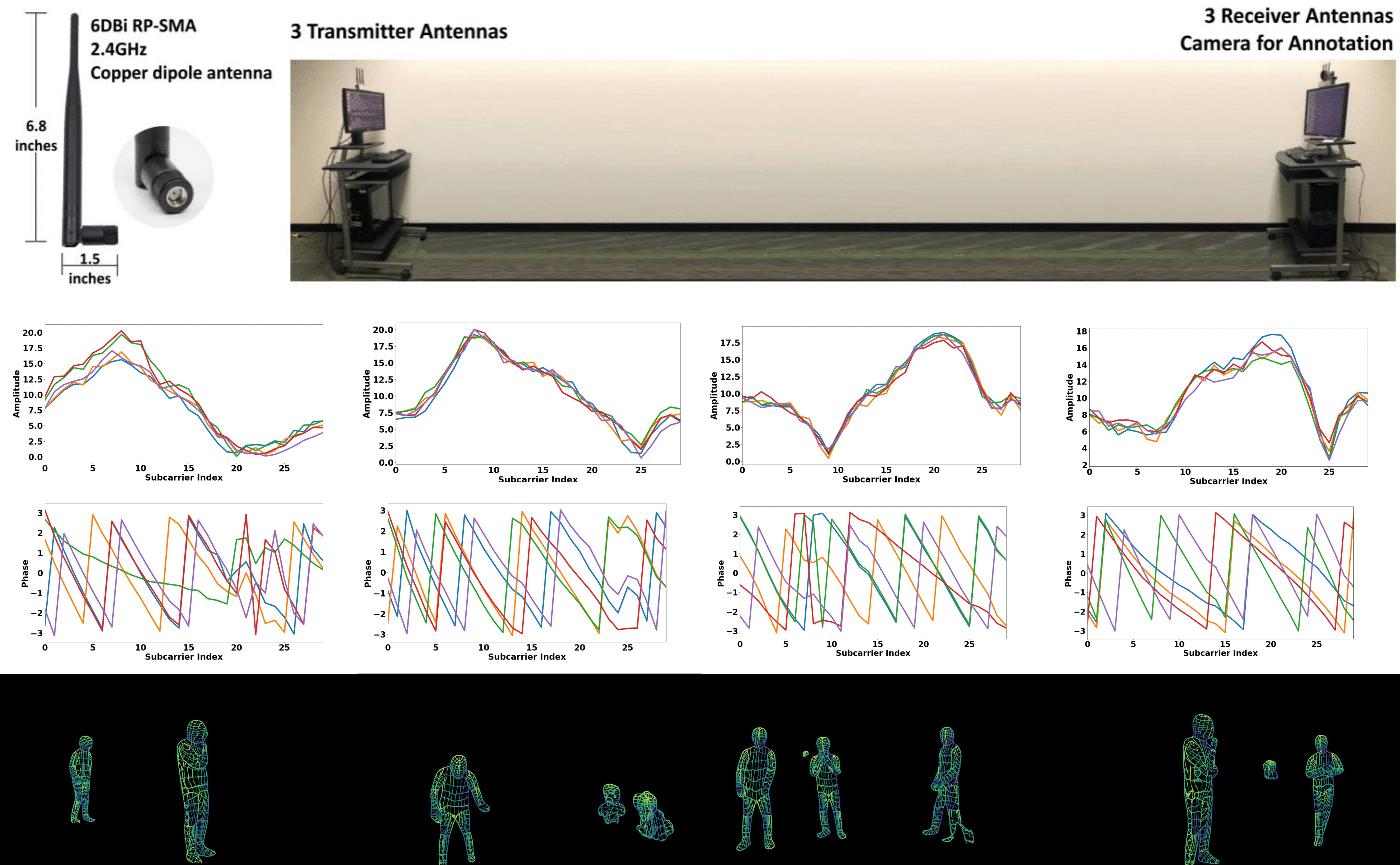
Figure 1. The first row illustrates the hardware setup. The second and third rows are the clips of amplitude and phase of the input WiFi signal. The fourth row contains the dense pose estimation of our algorithm from only the WiFi signal.

1. Introduction

Much progress has been made in human pose estimation using 2D (Güler et al., 2018; Wei et al., 2016; Sun et al., 2021; Kocabas et al., 2020; Saito et al., 2019; Cao et al., 2019) and 3D (Wang et al., 2018; Maturana and Scherer, 2015) sensors in the last few years (e.g., RGB sensors, LiDARs, radars), fueled by applications in autonomous driving and augmented reality. These traditional sensors, however, are constrained by both technical and practical considerations. LiDAR and radar sensors are frequently seen as being out of reach for the average household or small business due to their high cost. For example, the medium price of one of the most common COTS LiDAR, Intel L515, is around 700 dollars, and the prices for ordinary radar detectors range from 200 dollars to 600 dollars. In addition, these sensors are too power-consuming for daily and household use. As for RGB cameras, narrow field of view and poor lighting conditions, such as glare and darkness, can have a severe impact on camera-based approaches. Occlusion is another obstacle that prevents the camera-based model from generating reasonable pose predictions in images. This is especially worrisome for indoors scenarios, where furniture typically occludes people.

More importantly, privacy concerns prevent the use of these technologies in non-public places. For instance, most people are uncomfortable with having cameras recording them in their homes, and in certain areas (such as the bathroom) it will not be feasible to install them. These issues are particularly critical in healthcare applications, that are increasingly shifting from clinics to homes, where people are being monitored with the help of cameras and other sensors. It is important to resolve the aforementioned problems in order to better assist the aging population, which is the most susceptible (especially during COVID) and has a growing demand to keep them living independently at home.

We believe that WiFi signals can serve as a ubiquitous substitute for RGB images for human sensing in certain instances. Illumination and occlusion have little effect on WiFi-based solutions used for interior monitoring. In addition, they protect individuals’ privacy and the required equipment can be bought at a reasonable price. In fact, most households in developed countries already have WiFi at home, and this technology may be scaled to monitor the well-being of elder people or just identify suspicious behaviors at home.

The issue we are trying to solve is depicted in Fig. 1 (first row). Given three WiFi transmitters and three aligned receivers, can we detect and recover dense human pose correspondence in cluttered scenarios with multiple people (Fig. 1 fourth row). It should be noted that many WiFi routers, such as TP-Link AC1750, come with 3 antennas, so our method only requires 2 of these routers. Each of these router is around 30 dollars, which means our entire setup is still way cheaper than LiDAR and radar systems. Many factors make this a difficult task to solve. First of all, WiFi-based perception(Wang et al., 2019b; Kefayati et al., 2020) is based on the Channel-state-information (CSI) that represents the ratio between the transmitted signal wave and the received signal wave. The CSIs are complex decimal sequences that do not have spatial correspondence to spatial locations, such as the image pixels. Secondly, classic techniques rely on accurate measurement of time-of-fly and angle-of-arrival of the signal between the transmitter and receiver (Soltanaghaei et al., 2018a; Ledergerber and D’Andrea, 2019). These techniques only locate the object’s center; moreover, the localization accuracy is only around $0.5$ meters due to the random phase shift allowed by the IEEE 802.11n/ac WiFi communication standard and potential interference with electronic devices under similar frequency range such as microwave oven and cellphones.

To address these issues, we derive inspiration from recent proposed deep learning architectures in computer vision, and propose a neural network architecture that can perform dense pose estimation from WiFi. Fig 1 (bottom row) illustrates how our algorithm is able to estimate dense pose using only WiFi signal in scenarios with occlusion and multiple people.

2. Related Work

This section briefly describes existing work on dense estimation from images and human sensing from WiFi.

Our research aims to conduct dense pose estimation via WiFi. In computer vision, the subject of dense pose estimation from pictures and video has received a lot of attention (Güler et al., 2018; Neverova et al., 2020; Bristow et al., 2015; Zhou et al., 2016). This task consists of finding the dense correspondence between image pixels and the dense vertices indexes of a 3D human body model. The pioneering work of Güler et al. (Güler et al., 2018) mapped human images to dense correspondences of a human mesh model using deep networks. DensePose is based on instance segmentation architectures such as Mark-RCNN (He et al., 2017), and predicts body-wise UV maps for each pixel, where UV maps are flattened representations of 3d geometry, with coordinate points usually corresponding to the vertices of a 3d dimensional object. In this work, we borrow the same architecture as DensePose (Güler et al., 2018); however, our input will not be an image or video, but we use 1D WiFi signals to recover the dense correspondence.

Recently, there have been many extensions of DensePose proposed, especially in 3D human reconstruction with dense body parts (Xu et al., 2019; Alldieck et al., 2019; Yao et al., 2019; Zhang et al., 2020). Shapovalov et al.’s (Shapovalov et al., 2021) work focused on lifting dense pose surface maps to 3D human models without 3D supervision. Their network demonstrates that the dense correspondence alone (without using full 2D RGB images) contains sufficient information to generate posed 3D human body. Compared to previous works on reconstructing 3D humans with sparse 2D keypoints, DensePose annotations are much denser and provide information about the 3D surface instead of 2D body joints.

While there is a extensive literature on detection (Ren et al., 2015a; Redmon and Farhadi, 2018), tracking (Andriluka et al., 2018; Xiao et al., 2018), and dense pose estimation (Güler et al., 2018; Neverova et al., 2020) from images and videos, human pose estimation from WiFi or radar is a relatively unexplored problem. At this point, it is important to differentiate the current work on radar-based systems and WiFi. The work of Adib et.al. (Adib et al., 2014) proposed a Frequency Modulated Continuous Wave (FMCW) radar system (broad bandwidth from 5.56GHz to 7.25GHz) for indoor human localization. A limitation of this system is the specialized hardware for synchronizing the transmission, refraction, and reflection to compute the Time-of-Flight (ToF). The system reached a resolution of 8.8 cm on body localization. In the following work (Adib et al., 2015), they improved the system by focusing on a moving person and generated a rough single-person outline with depth maps. Recently, they applied deep learning approaches to do fine-grained human pose estimation using a similar system, named RF-Pose (Zhao et al., 2018). These systems do not work under the IEEE 802.11n/ac WiFi communication standard (40MHz bandwidth centered at 2.4GHz). They rely on additional high-frequency and high-bandwidth electromagnetic fields, which need specialized technology not available to the general public. Recently, significant improvements have been made to radar-based human sensing systems. mmMesh (Xue et al., 2021) generates 3D human mesh from commercially portable millimeter-wave devices. This system can accurately localize the vertices on the human mesh with an average error of 2.47 cm. However, mmMesh does not work well with occlusions since high-frequency radio waves cannot penetrate objects.

Unlike the above radar systems, the WiFi-based solution (Wang et al., 2019b; Kefayati et al., 2020) used off-the-shelf WiFi adapters and 3dB omnidirectional antennas. The signal propagate as the IEEE 802.11n/ac WiFi data packages transmitting between antennas, which does not introduce additional interference. However, WiFi-based person localization using the traditional time-of-flight (ToF) method is limited by its wavelength and signal-to-noise ratio. Most existing approaches only conduct center mass localization (BASRI and Khadimi, 2016; Soltanaghaei et al., 2018b) and single-person action classification (Sheng et al., 2020; Wang et al., 2019a). Recently, Fei Wang et.al. (Wang et al., 2019c) demonstrated that it is possible to detect $17$ 2D body joints and perform 2D semantic body segmentation mask using only WiFi signals. In this work, we go beyond (Wang et al., 2019c) by estimating dense body pose, with much more accuracy than the 0.5m that the WiFi signal can provide theoretically. Our dense posture outputs push above WiFi’s signal constraint in body localization, paving the road for complete dense 2D and possibly 3D human body perception through WiFi. To achieve this, instead of directly training a randomly initialized WiFi-based model, we explored rich supervision information to improve both the performance and training efficiency, such as utilizing the CSI phase, adding keypoint detection branch, and transfer learning from the image-based model.

3. Methods

Our approach produces UV coordinates of the human body surface from WiFi signals using three components: first, the raw CSI signals are cleaned by amplitude and phase sanitization. Then, a two-branch encoder-decoder network performs domain translation from sanitized CSI samples to 2D feature maps that resemble images. The 2D features are then fed to a modified DensePose-RCNN architecture (Güler et al., 2018) to estimate the UV map, a representation of the dense correspondence between 2D and 3D humans. To improve the training of our WiFi-input network, we conduct transfer learning, where we minimize the differences between the multi-level feature maps produced by images and those produced by WiFi signals before training our main network.

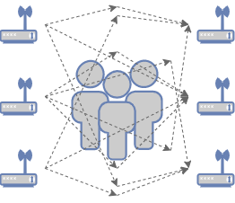
(a) Layout of WiFi devices and human bodies

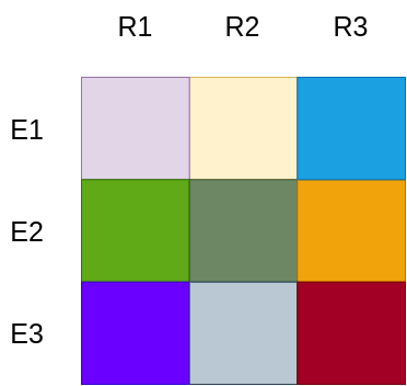
(b) The $3\times 3$ dimensions of the CSI tensor

Figure 2. CSI samples from Wifi. (a) the layout of WiFi devices and human bodies, and (b) the $3\times 3$ tensor dimension corresponds to the $3\times 3$ transmitter-receiver antenna pairs. For instance, $E1$ denotes the first emitter and $R1$ denotes the first receiver, etc. By incorporating the 5 consecutive complex-valued CSI samples (100 samples/second) under 30 subcarrier frequencies, the two input tensors to our network are a $150\times 3\times 3$ amplitude tensor and a $150\times 3\times 3$ phase tensor.

The raw CSI data are sampled in 100Hz as complex values over 30 subcarrier frequencies (linearly spaced within 2.4GHz$\pm$20MHz) transmitting among 3 emitter antennas and 3 reception antennas (see Figure 2). Each CSI sample contains a $3\times 3$ real integer matrix and a $3\times 3$ imaginary integer matrix. The inputs of our network contained 5 consecutive CSI samples under 30 frequencies, which are organized in a $150\times 3\times 3$ amplitude tensor and a $150\times 3\times 3$ phase tensor respectively. Our network outputs include a $17\times 56\times 56$ tensor of keypoint heatmaps (one $56\times 56$ map for each of the 17 kepoints) and a $25\times 112\times 112$ tensor of UV maps (one $112\times 112$ map for each of the 24 body parts with one additional map for background).

3.1. Phase Sanitization

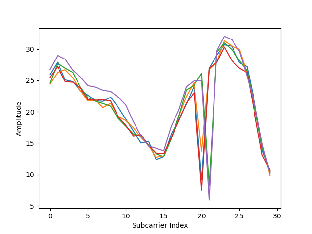
(a) Original CSI Amplitude

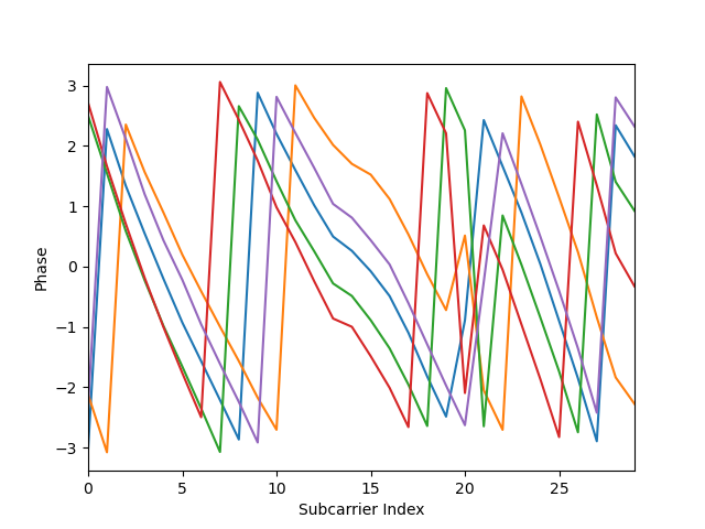
(b) Original CSI Phase

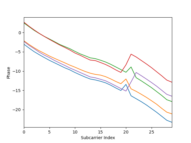
(c) Phase after unwrapping

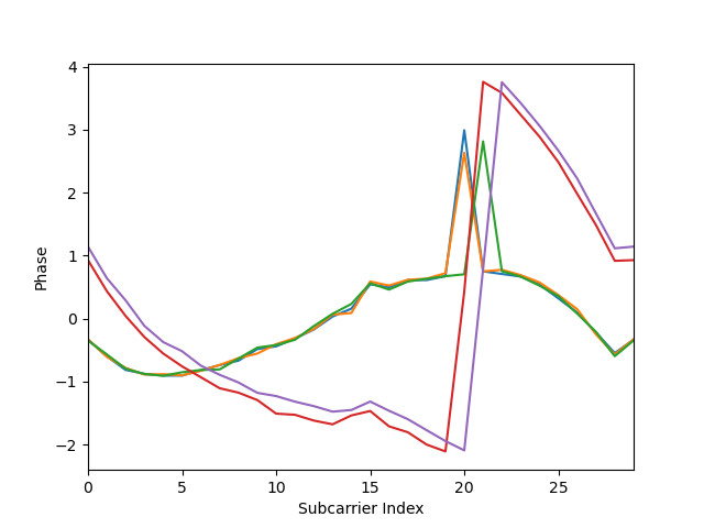
(d) Phase after unwrapping + linear fitting

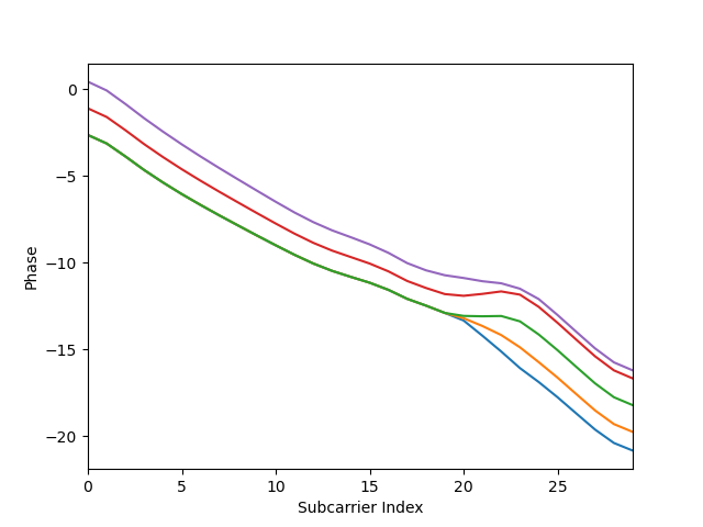
(e) Phase after unwrapping + filtering

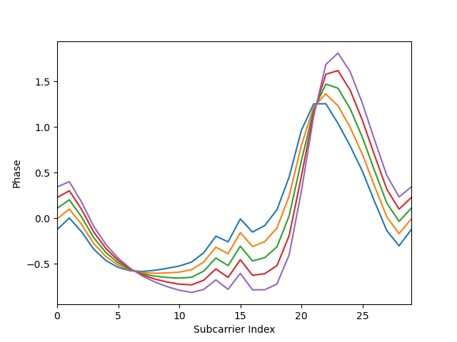
(f) Phase after unwrapping + filtering + linear fitting

Figure 3. Sanitization steps of CSI sequences described in Section 3.1. In each subfigure, we plot five consecutive samples (five colored curves) each containing CSI data of 30 IEEE 802.11n/ac sub-Carrier frequencies (horizontal axis).

The raw CSI samples are noisy with random phase drift and flip (see Figure 3(b)). Most WiFi-based solutions disregard the phase of CSI signals and rely only on their amplitude (see Figure 3 (a)). As shown in our experimental validation, discarding the phase information have a negative impact on the performance of our model. In this section, we perform sanitization to obtain stable phase values to enable full use of the CSI information.

In raw CSI samples (5 consecutive samples visualized in Figure 3(a-b)), the amplitude ($A$) and phase ($\Phi$) of each complex element $z=a+bi$ are computed using the formulation $A=\sqrt{(a^{2}+b^{2})}$ and $\Phi=arctan(b/a)$. Note that the range of the $\arctan$ function is from $-\pi$ to $\pi$ and the phase values outside this range get wrapped, leading to a discontinuity in phase values. Our first sanitization step is to unwrap the phase following (Jiang et al., 2017):

(1) $$\Delta\phi_{i,j} =\Phi_{i,j+1}-\Phi_{i,j}$$

$$\text{if }\Delta\phi_{i,j}>\pi,\Phi_{i,j+1} =\Phi_{i,j}+\Delta\phi_{i,j}-2\pi$$

$$\text{if }\Delta\phi_{i,j}<-\pi,\Phi_{i,j+1} =\Phi_{i,j}+\Delta\phi_{i,j}+2\pi,$$

where $i$ denotes the index of the measurements in the five consecutive samples, and $j$ denotes the index of the subcarriers(frequencies). Following unwrapping, each of the flipping phase curves in Figure 3(b) are restored to continuous curves in Figure 3(c).

Observe that among the 5 phase curves captured in 5 consecutive samples in Figure 3(c), there are random jiterings that break the temporal order among the samples. To keep the temporal order of signals, previous work (Sen et al., 2012) mentioned linear fitting as a popular approach. However, directly applying linear fitting to Figure 3(c) further amplified the jitering instead of fixing it (see the failed results in Figure 3(d)).

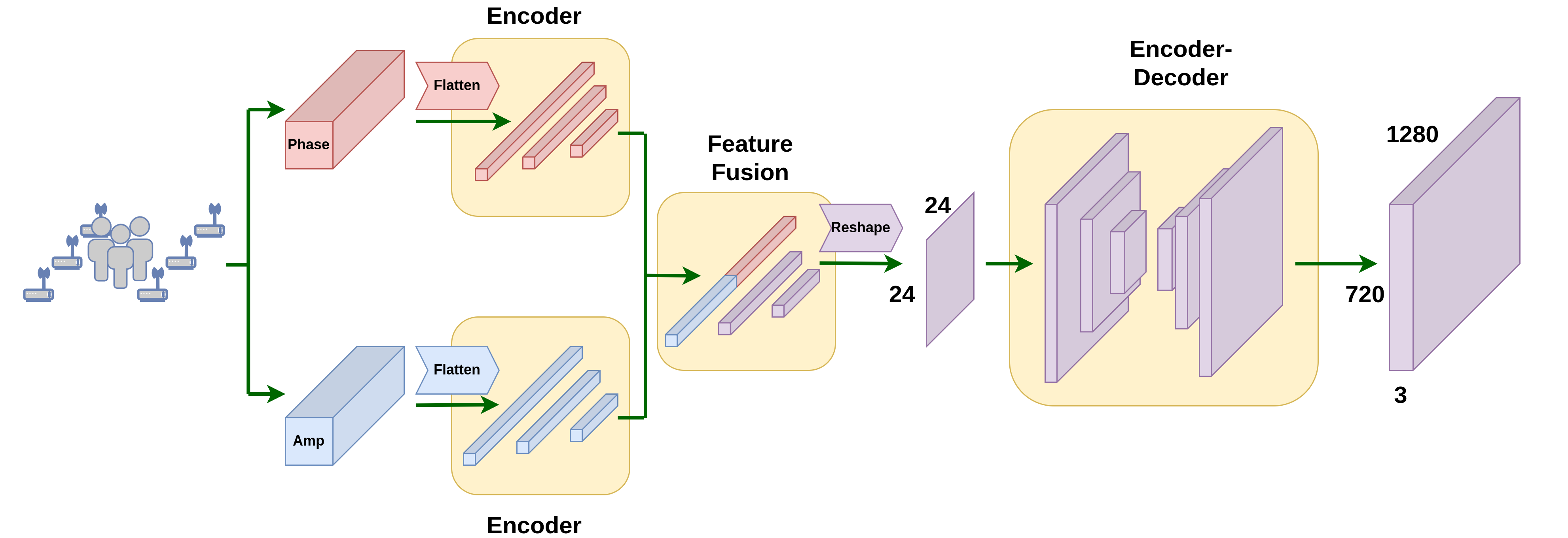
Figure 4. Modality Translation Network. Two encoders extract the features from the amplitude and phase in the CSI domain. Then the features are fused and reshaped before going through an encoder-decoder network. The output is a $3\times 720\times 1280$ feature map in the image domain.

From Figure 3(c), we use median and uniform filters to eliminate outliers in both the time and frequency domain which leads to Figure 3(e). Finally, we obtain the fully sanitized phase values by applying the linear fitting method following the equations below:

(2) $$\alpha_{1} =\frac{\Phi_{F}-\Phi_{1}}{2\pi F}$$

$$\alpha_{0} =\frac{1}{F}\sum_{1\leq f\leq F}\phi_{f}$$

$$\hat{\phi_{f}} =\phi_{f}-(\alpha_{1}f+a_{0}),$$

where $F$ denotes the largest subcarrier index (30 in our case) and $\hat{\phi_{f}}$ is the sanitized phase values at subcarrier $f$ (the $f$th frequency). In Figure 3(f), the final phase curves are temporally consistent.

3.2. Modality Translation Network

In order to estimate the UV maps in the spatial domain from the 1D CSI signals, we first transform the network inputs from the CSI domain to the spatial domain. This is done with the Modality Translation Network (see Figure 4). We first extract the CSI latent space features using two encoders, one for the amplitude tensor and the other for the phase tensor, where both tensors have the size of $150\times 3\times 3$ (5 consecutive samples, 30 frequencies, 3 emitters and 3 receivers). Previous work on human sensing with WiFi (Wang et al., 2019b) stated that Convolutional Neural Network (CNN) can be used to extract spatial features from the last two dimensions (the $3\times 3$ transmitting sensor pairs) of the input tensors. We, on the other hand, believe that locations in the $3\times 3$ feature map do not correlate with the locations in the 2D scene. More specifically, as depicted in Figure 2(b), the element that is colored in blue represents a 1D summary of the entire scene captured by emitter 1 and receiver 3 (E1 - R3), instead of local spatial information of the top right corner of the 2D scene. Therefore, we consider that each of the 1350 elements (in both tensors) captures a unique 1D summary of the entire scene. Following this idea, the amplitude and phase tensors are flattened and feed into two separate multi-layer perceptrons (MLP) to obtain their features in the CSI latent space. We concatenated the 1D features from both encoding branches, then the combined tensor is fed to another MLP to perform feature fusion.

The next step is to transform the CSI latent space features to feature maps in the spatial domain. As shown in Figure 4, the fused 1D feature is reshaped into a $24\times 24$ 2D feature map. Then, we extract the spatial information by applying two convolution blocks and obtain a more condensed map with the spatial dimension of $6\times 6$. Finally, four deconvolution layers are used to upsample the encoded feature map in low dimensions to the size of $3\times 720\times 1280$. We set such an output tensor size to match the dimension commonly used in RGB-image-input network. We now have a scene representation in the image domain generated by WiFi signals.

3.3. WiFi-DensePose RCNN

After we obtain the $3\times 720\times 1280$ scene representation in the image domain, we can utilize image-based methods to predict the UV maps of human bodies. State-of-the-art pose estimation algorithms are two-stage; first, they run an independent person detector to estimate the bounding box and then conduct pose estimation from person-wise image patches. However, as stated before, each element in our CSI input tensors is a summary of the entire scene. It is not possible to extract the signals corresponding to a single person from a group of people in the scene. Therefore, we decide to adopt a network structure similar to DensePose-RCNN (Güler et al., 2018), since it can predict the dense correspondence of multiple humans in an end-to-end fashion.

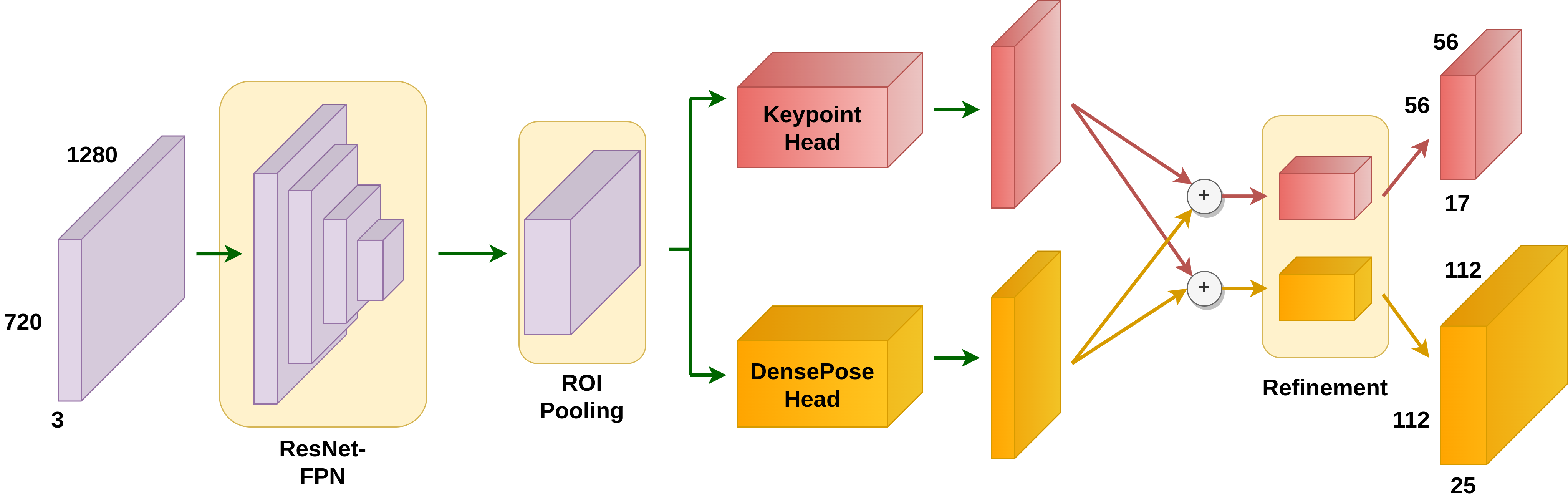
Figure 5. WiFi-DensePose RCNN. The $3\times 720\times 1280$ feature map from Figure 4 first goes through standard ResNet-FPN and ROI pooling to extract person-wise features. The features are then processed by two heads:the Keypoint Head and the DensePose Head.

More specifically, in the WiFi-DensePose RCNN (Figure 5), we extract the spatial features from the obtained $3\times 720\times 1280$ image-like feature map using the ResNet-FPN backbone (Lin et al., 2016). Then, the output will go through the region proposal network (Ren et al., 2015a). To better exploit the complementary information of different sources, the next part of our network contains two branches: DensePose head and Keypoint head. Estimating keypoint locations is more reliable than estimating dense correspondences, so we can train our network to use keypoints to restrict DensePose predictions from getting too far from the body joints of humans. The DensePose head utilizes a Fully Convolutional Network (FCN) (Long et al., 2014) to densely predict human part labels and surface coordinates (UV coordinates) within each part, while the keypoint head uses FCN to estimate the keypoint heatmap. The results are combined and then fed into the refinement unit of each branch, where each refinement unit consists of two convolutional blocks followed by an FCN. The network outputs a $17\times 56\times 56$ keypoint mask and a $25\times 112\times 112$ IUV map. The process is demonstrated in Figure 5. It should be noted that the modality translation network and the WiFi-DensePose RCNN are trained together.

3.4. Transfer Learning

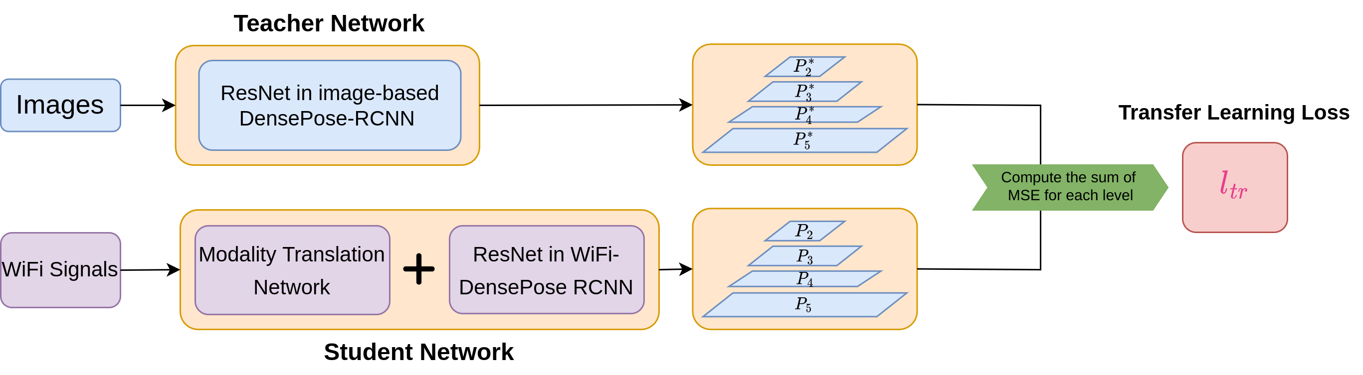
Figure 6. Transfer learning from an image-based teacher network to our WiFi-based network.

Training the Modality Translation Network and WiFi-DensePose RCNN network from a random initialization takes a lot of time (roughly 80 hours). To improve the training efficiency, we conduct transfer learning from an image-based DensPose network to our WiFi-based network (See Figure 6 for details).

The idea is to supervise the training of the WiFi-based network with the pre-trained image-based network. Directly initializing the WiFi-based network with image-based network weights does not work because the two networks get inputs from different domains (image and channel state information). Instead, we first train an image-based DensePose-RCNN model as a teacher network. Our student network consists of the modality translation network and the WiFi-DensePose RCNN. We fix the teacher network weights and train the student network by feeding them with the synchronized images and CSI tensors, respectively. We update the student network such that its backbone (ResNet) features mimic that of our teacher network. Our transfer learning goal is to minimize the differences of multiple levels of feature maps generated by the student model and those generated by the teacher model. Therefore we calculate the mean squared error between feature maps. The transfer learning loss from the teacher network to the student network is:

(3) $$L_{tr}=MSE(P_{2},P^{*}_{2})+MSE(P_{3},P^{*}_{3})+MSE(P_{4},P^{*}_{4})+MSE(P_{5},P^{*}_{5}),$$

where $MSE(\cdot)$ computes the mean squared error between two feature maps, $\{P_{2},P_{3},P_{4},P_{5}\}$ is a set of feature maps produced by the teacher network (Lin et al., 2016), and $\{P^{*}_{2},P^{*}_{3},P^{*}_{4},P^{*}_{5}\}$ is the set of feature maps produced by the student network (Lin et al., 2016).

Benefiting from the additional supervision from the image-based model, the student network gets higher performance and takes fewer iterations to converge (Please see results in Table 5).

3.5. Losses

The total loss of our approach is computed as:

$$L = L_{cls}+L_{box}+\lambda_{dp}L_{dp}+\lambda_{kp}L_{kp}+\lambda_{tr}L_{tr},$$

where $L_{cls},L_{box},L_{dp},L_{kp},L_{tr}$ are losses for the person classification, bounding box regression, DensePose, keypoints, and transfer learning respectively. The classification loss $L_{cls}$ and the box regression loss $L_{box}$ are standard RCNN losses (Ren et al., 2015b; He et al., 2017). The DensePose loss $L_{dp}$(Güler et al., 2018) consists of several sub-components: (1) Cross-entropy loss for the coarse segmentation tasks. Each pixel is classified as either belonging to the background or one of the 24 human body regions. (2) Cross-entropy loss for body part classification and smooth L1 loss for UV coordinate regression. These losses are used to determine the exact coordinates of the pixels, i.e., 24 regressors are created to break the full human into small parts and parameterize each piece using a local two-dimensional UV coordinate system, that identifies the position UV nodes on this surface part.

We add $L_{kp}$ to help the DensePose to balance between the torso with more UV nodes and limbs with fewer UV nodes. Inspired by Keypoint RCNN (He et al., 2017), we one-hot-encode each of the $17$ ground truth keypoints in one $56\times 56$ heatmap, generating $17\times 56\times 56$ keypoints heatmaps and supervise the output with the Cross-Entropy Loss. To closely regularize the Densepose regression, the keypoint heatmap regressor takes the same input features used by the Denspose UV maps.

4. Experiments

This section presents the experimental validation of our WiFi-based DensePose.

4.1. Dataset

We used the dataset described in (Wang et al., 2019c), which contains CSI samples taken at $100$Hz from receiver antennas and videos recorded at $20$ FPS. Time stamps are used to synchronize CSI and the video frames such that 5 CSI samples correspond to 1 video frame. The dataset was gathered in sixteen spatial layouts: six captures in the lab office and ten captures in the classroom. Each capture is around 13 minutes with 1 to 5 subjects (8 subjects in total for the entire dataset) performing daily activities under the layout described in Figure 2 (a). The sixteen spatial layouts are different in their relative locations/orientations of the WiFi-emitter antennas, person, furniture, and WiFi-receiver antennas.

There are no manual annotations for the data set. We use the MS-COCO-pre-trained dense model ”R_101_FPN_s1x_legacy” and MS-COCO-pre-trained Keypoint R-CNN ”R101-FPN” to produce the pseudo ground truth. We denote the ground truth as ”R101-Pseudo-GT” (see an annotated example in Figure 7). The R101-Pseudo-GT includes person bounding boxes, person-instance segmentation masks, body-part UV maps, and person-wise keypoint coordinates.

Throughout the section, we use R101-Puedo-GT to train our WiFi-based DensePose model as well as finetuning the image-based baseline ”R_50_FPN_s1x_legacy”.

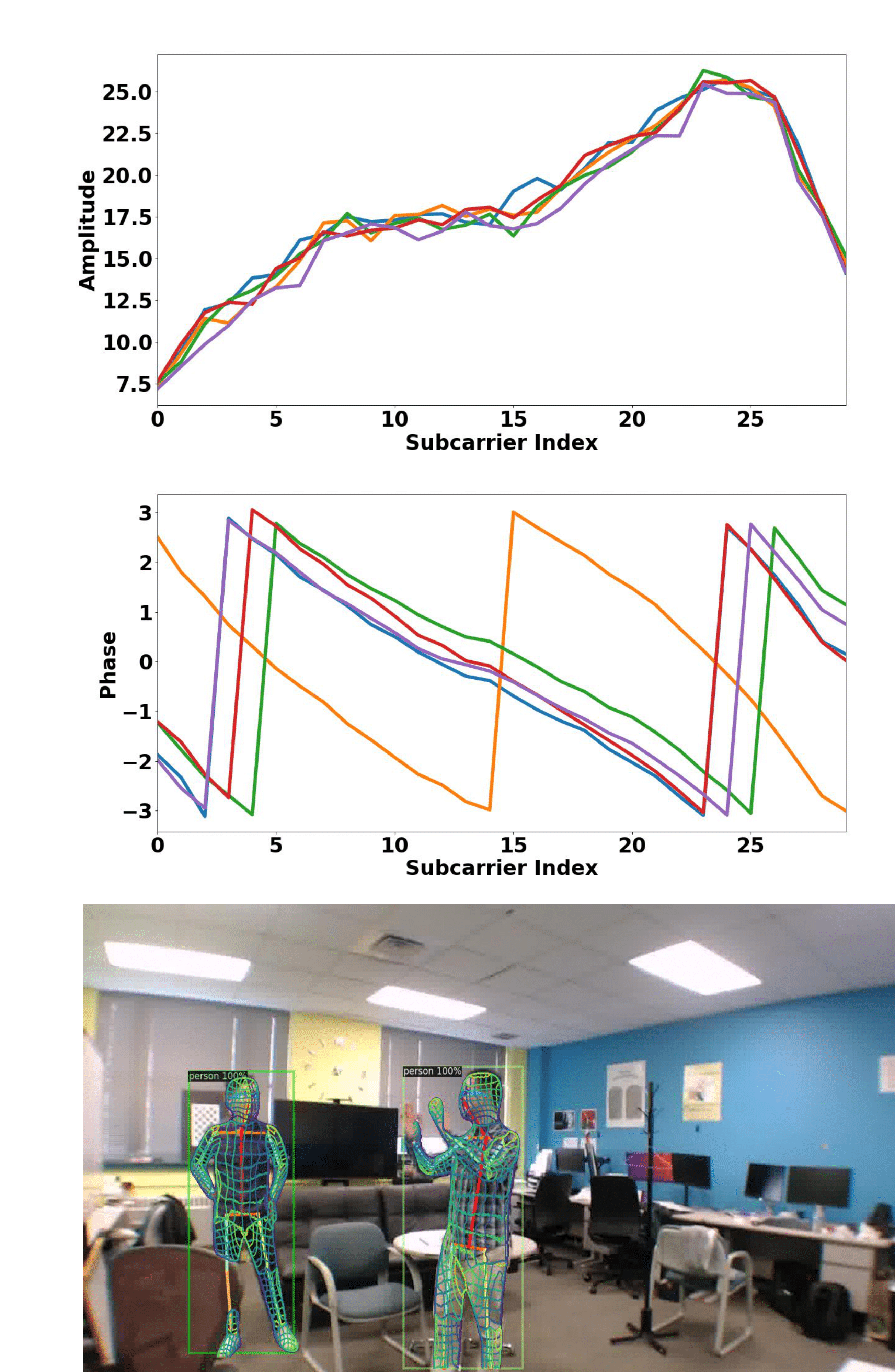
Figure 7. Top two rows are the amplitude and phase of the input WiFi signal. The bottom row shows R101-Psuedo-GT: the ground truth dense pose and keypoints annotated by running a pretrained image-based Densepose network on the corresponding RGB image (see Section 4.1 for details).

4.2. Training/Testing protocols and Metrics

We report results on two protocols: (1) Same layout: We train on the training set in all $16$ spatial layouts, and test on remaining frames. Following (Wang et al., 2019c), we randomly select 80$\%$ of the samples to be our training set, and the rest to be our testing set. The training and testing samples are different in the person’s location and pose, but share the same person’s identities and background. This is a reasonable assumption since the WiFi device is usually installed in a fixed location. (2) Different layout: We train on 15 spatial layouts and test on 1 unseen spatial layout. The unseen layout is in the classroom scenarios.

We evaluate the performance of our algorithm in two aspects: the ability to detect humans (bounding boxes) and accuracy of the dense pose estimation.

To evaluate the performance of our models in detecting humans, we calculate the standard average precision (AP) of person bounding boxes at multiple IOU thresholds ranging from 0.5 to 0.95.

In addition, by MS-COCO (Lin et al., 2014) definition, we also compute AP-m for median bodies that are enclosed in bounding boxes with sizes between $32\times 32$ and $96\times 96$ pixels in a normalized $640\times 480$ pixels image space, and AP-l for large bodies that are enclosed in bounding boxes larger than $96\times 96$ pixels.

To measure the performance of DensePose detection, we follow the original DensePose paper (Güler et al., 2018). We first compute Geodesic Point Similarity (GPS) as a matching score for dense correspondences:

(4) $$GPS_{j}=\frac{1}{|P_{j}|}\sum_{p\in P_{j}}\exp(\frac{-g(i_{p},\hat{i}_{p})^{2}}{2\kappa^{2}}),$$

where $g$ calculates the geodesic distance, $P_{j}$ denotes the ground truth point annotations of person $j$, $i_{p}$ and $\hat{i}_{p}$ are the estimated and ground truth vertex at point $p$ respectively, and $\kappa$ is a normalizing parameter (set to be 0.255 according to (Güler et al., 2018)).

One issue of GPS is that it does not penalize spurious predictions. Therefore, estimations with all pixels classified as foreground are favored. To alleviate this issue, masked geodesic point similarity (GPSm) was introduced in (Güler et al., 2018), which incorporates both GPS and segmentation masks. The formulation is as follows:

(5) $$GPSm=\sqrt{GPS\cdot I},I=\frac{M\cap\hat{M}}{M\cup\hat{M}},$$

where $M$ and $\hat{M}$ are the predicted and ground truth foreground segmentation masks.

Next, we can calculate DensePose average precision with GPS (denoted as dpAP$\cdot$ GPS) and GPSm (denoted as dpAP$\cdot$ GPSm) as thresholds, following the same logic behind the calculation of bounding box AP.

4.3. Implementation Details

We implemented our approach in PyTorch. We set the training batch size to 16 on a 4 GPU (Titan X) server. We empirically set $\lambda_{dp}=0.6,\lambda_{kp}=0.3,\lambda_{tr}=0.1$. We used a warmup multi-step learning rate scheduler and set the initial learning rate as $1e-5$. The learning rate increases to $1e-3$ during the first 2000 iterations, then decreases to $\frac{1}{10}$ of its value every 48000 iterations. We trained for $145,000$ iterations for our final model.

4.4. WiFi-based DensePose under Same Layout

Under the Same Layout protocol, we compute the AP of human bounding box detections as well as dpAP$\cdot$ GPS and dpAP$\cdot$ GPSm of dense correspondence predictions. Results are presented in Table 1 and Table 2, respectively.

Method	AP	AP@50	AP@75	AP-m	AP-l
WiFi	43.5	87.2	44.6	38.1	46.4

Table 1. Average precision (AP) of WiFi-based DensePose under the Same Layout protocol. All metrics are the higher the better.

From Table 1, we can observe a high value (87.2) of AP@50, indicating that our model can effectively detect the approximate locations of human bounding boxes. The relatively low value (35.6) for AP@75 suggests that the details of the human bodies are not perfectly estimated.

Method	dpAP $\cdot$ GPS	dpAP $\cdot$ GPS@50	dpAP $\cdot$ GPS@75	dpAP $\cdot$ GPSm	dpAP $\cdot$ GPSm@50	dpAP $\cdot$ GPSm@75
WiFi	45.3	76.7	47.7	44.8	73.6	44.9

Table 2. DensePose Average precision (dpAP $\cdot$ GPS, dpAP $\cdot$ GPSm) of WiFi-based DensePose under the Same Layout protocol. All metrics are the higher the better.

A similar pattern can be seen from the results of DensePose estimations (see Table 2 for details). Experiments report high values of dpAP $\cdot$ GPS@50 and dpAP $\cdot$ GPSm@50, but low values of dpAP $\cdot$ GPS@75 and dpAP $\cdot$ GPSm@75. This demonstrates that our model performs well at estimating the poses of human torsos, but still struggles with detecting details like limbs.

4.5. Comparison with Image-based DensePose

Method	AP	AP@50	AP@75	AP-m	AP-l
WiFi	43.5	87.2	44.6	38.1	46.4
Image	84.7	94.4	77.1	70.3	83.8

Table 3. Average precision (AP) of WiFi-based and image-based DensePose under the Same Layout protocol. All metrics are the higher the better.

As discussed in Section 4.1, since there are no manual annotations on the WiFi dataset, it is difficult to compare the performance of WiFi-based DensePose with its Image-based counterpart. This is a common drawback of many WiFi perception works including (Wang et al., 2019c).

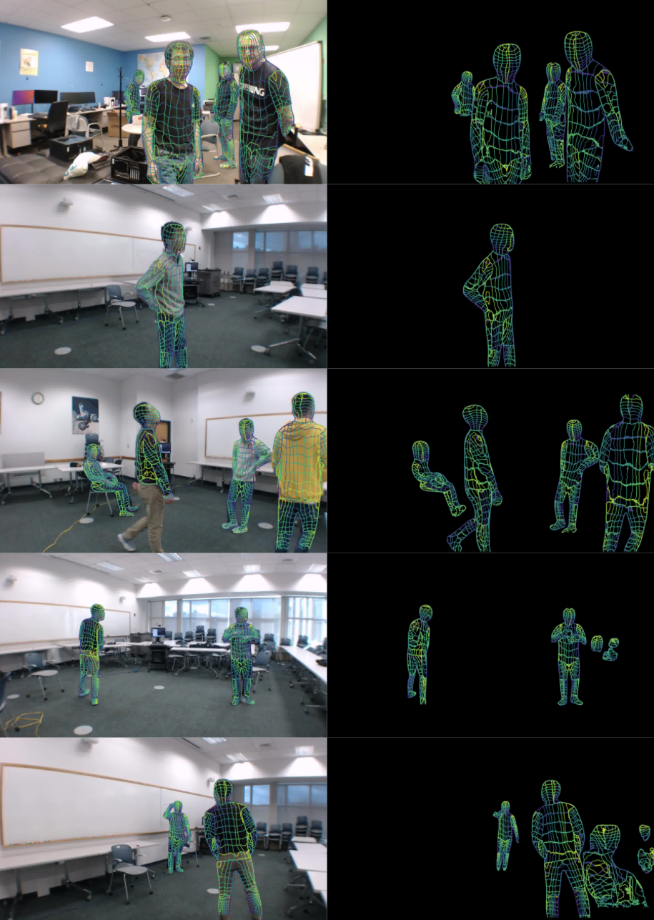
Figure 10. More qualitative comparison using synchronized images and WiFi signals. (Left Column) image-based DensePose (Right Column) our WiFi-based DensePose.

Nevertheless, conducting such a comparison is still worthwhile in assessing the current limit of WiFi-based perception. We tried an image-based DensePose baseline ”R_50_FPN_s1x_legacy” finetuned on R101-Pseudo-GT under the Same Layout protocol. In addition, as shown in Figure 9 and Figure 10, though certain defects still exist, the estimations from our WiFi-based model are reasonably well compared to the results produced by Image-based DensePose.

In the quantitative results in Table 3 and Table 4, the image-based baseline produces very high APs due to the small difference between its ResNet50 backbone and the Resnet101 backbone used to generate R101-Pseudo-GT. This is to be expected. Our WiFi-based model has much lower absolute metrics. However, it can be observed from Table 3 that the difference between AP-m and AP-l values is relatively small for the WiFi-based model. We believe this is because individuals who are far away from cameras occupy less space in the image, which leads to less information about these subjects. On the contrary, WiFi signals incorporate all the information in the entire scene, regardless of the subjects’ locations.

Method	dpAP $\cdot$ GPS	dpAP $\cdot$ GPS@50	dpAP $\cdot$ GPS@75	dpAP $\cdot$ GPSm	dpAP $\cdot$ GPSm@50	dpAP $\cdot$ GPSm@75
WiFi	45.3	79.3	47.7	43.2	77.4	45.5
Image	81.8	93.7	86.2	84.0	94.9	86.8

Table 4. DensePose Average precision (dpAP $\cdot$ GPS, dpAP $\cdot$ GPSm) of WiFi-based and image-based DensePose under the Same Layout protocol. All metrics are the higher the better.

Method	AP	AP@50	AP@75	AP-m	AP-l	Number of Trained Iterations
Amplitude-only Model	39.5	85.4	41.3	34.4	43.7	174000
+ Sanitized Phase Input	40.3	85.9	41.9	34.6	44.5	180000
+ Keypoint Supervision	42.9	86.8	44.1	38.0	45.8	186000
+ Transfer Learning	43.5	87.2	44.6	38.1	46.4	145000

Table 5. Ablation study of human detection under the Same-layout protocol. All metrics are the higher the better.

Method	dpAP $\cdot$ GPS	dpAP $\cdot$ GPS@50	dpAP $\cdot$ GPS@75	dpAP $\cdot$ GPSm	dpAP $\cdot$ GPSm@50	dpAP $\cdot$ GPSm@75
Amplitude-only Model	40.6	76.6	41.5	39.7	75.1	40.3
+ Sanitized Phase Input	41.2	77.4	42.3	40.1	75.7	40.5
+ Keypoint Supervision	44.6	78.8	46.9	42.9	76.8	44.9
+ Transfer Learning	45.3	79.3	47.7	43.2	77.4	45.5

Table 6. Ablation study of DensePose estimation under the Same-layout protocol. All metrics are the higher the better.

4.6. Ablation Study

This section describes the ablation study to understand the effects of phase information, keypoint supervision, and transfer learning on estimating dense correspondences. Similar to section 4.4, the models analyzed in this section are all trained under the same-layout mentioned in section 4.2.

We start by training a baseline WiFi model, which does not include the phase encoder, the keypoint detection branch, or transfer learning. The results are presented in the first row of both Table 5 and Table 6 as a reference.

Addition of Phase information: We first examine whether the phase information can enhance the baseline performance. As shown in the second row of Table 5 and Table 6, the results for all the metrics have slightly improved from the baseline. This proves our hypothesis that the phase can reveal relevant information about the dense human pose.

Addition of a keypoint detection branch: Having established the advantage of incorporating phase information, we now evaluate the effect of adding a keypoint branch to our model. The quantitative results are summarized in the third row of Table 5 and Table 6.

Comparing with the numbers on the second row, we can observe a slight increase in performance in terms of dpAP$\cdot$GPS@50(from 77.4 to 78.8) and dpAP$\cdot$GPSm@50 (from 75.7 to 76.8), and a more noticeable improvement in terms of dpAP$\cdot$GPS@75 (from 42.3 to 46.9) and dpAP$\cdot$GPSm@75 (from 40.5 to 44.9). This indicates that the keypoint branch provides effective references to dense pose estimations, and our model becomes significantly better at detecting subtle details (such as the limbs).

Effect of Transfer Learning: We aim to reduce the training time for our model with the help of transfer learning. For each model in Table 5, we continue training the model until there are no significant changes in terms of performance. The last row of Table 5 and Table 6 represents our final model with transfer learning. Though the final performance does not improve too much compared to the model (with phase information and keypoints) without transfer learning, it should be noted that the number of training iterations decreases significantly from 186000 to 145000 (this number includes the time to perform transfer learning as well as training the main model).

4.7. Performance in different layouts

Method	AP	AP@50	AP@75	AP-m	AP-l
WiFi (base)	23.5	48.1	20.3	19.4	24.5
WiFi (final)	27.3	51.8	24.2	22.1	28.6
Image	60.6	80.4	52.1	48.3	65.8

Table 7. Average precision (AP) of WiFi-based and image-based DensePose under the Different Layout protocol. All metrics are the higher the better.

Method	dpAP $\cdot$ GPS	dpAP $\cdot$ GPS@50	dpAP $\cdot$ GPS@75	dpAP $\cdot$ GPSm	dpAP $\cdot$ GPSm@50	dpAP $\cdot$ GPSm@75
WiFi (base)	22.3	47.3	21.5	20.9	44.6	21.8
WiFi (final)	25.4	50.2	24.7	23.2	47.4	26.5
Image	60.2	70.1	62.3	54.0	72.7	58.8

Table 8. DensePose Average precision (dpAP $\cdot$ GPS, dpAP $\cdot$ GPSm) of WiFi-based and image-based DensePose under the Different Layout protocol. All metrics are the higher the better.

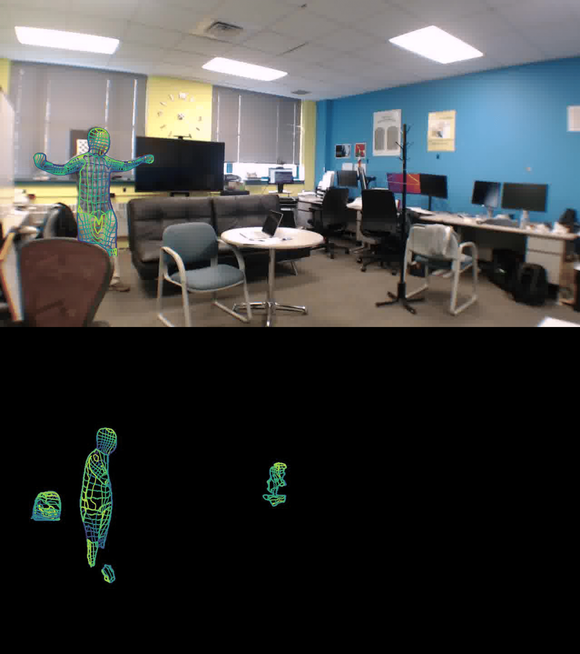
(a)

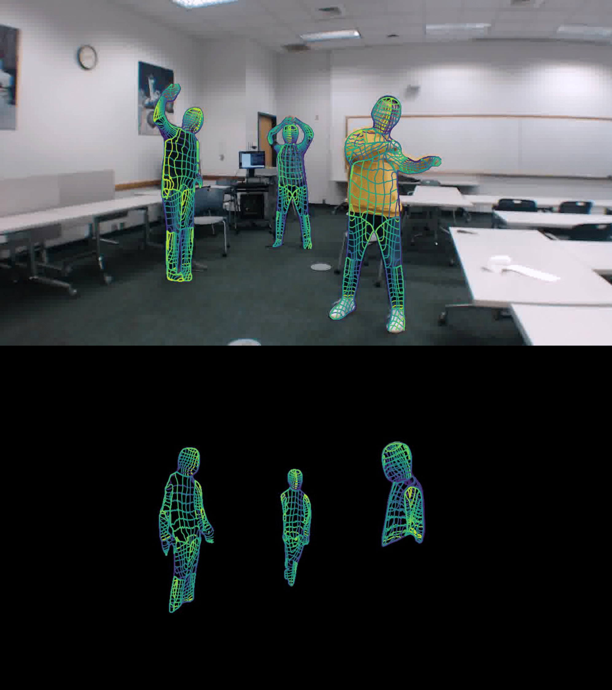
(b)

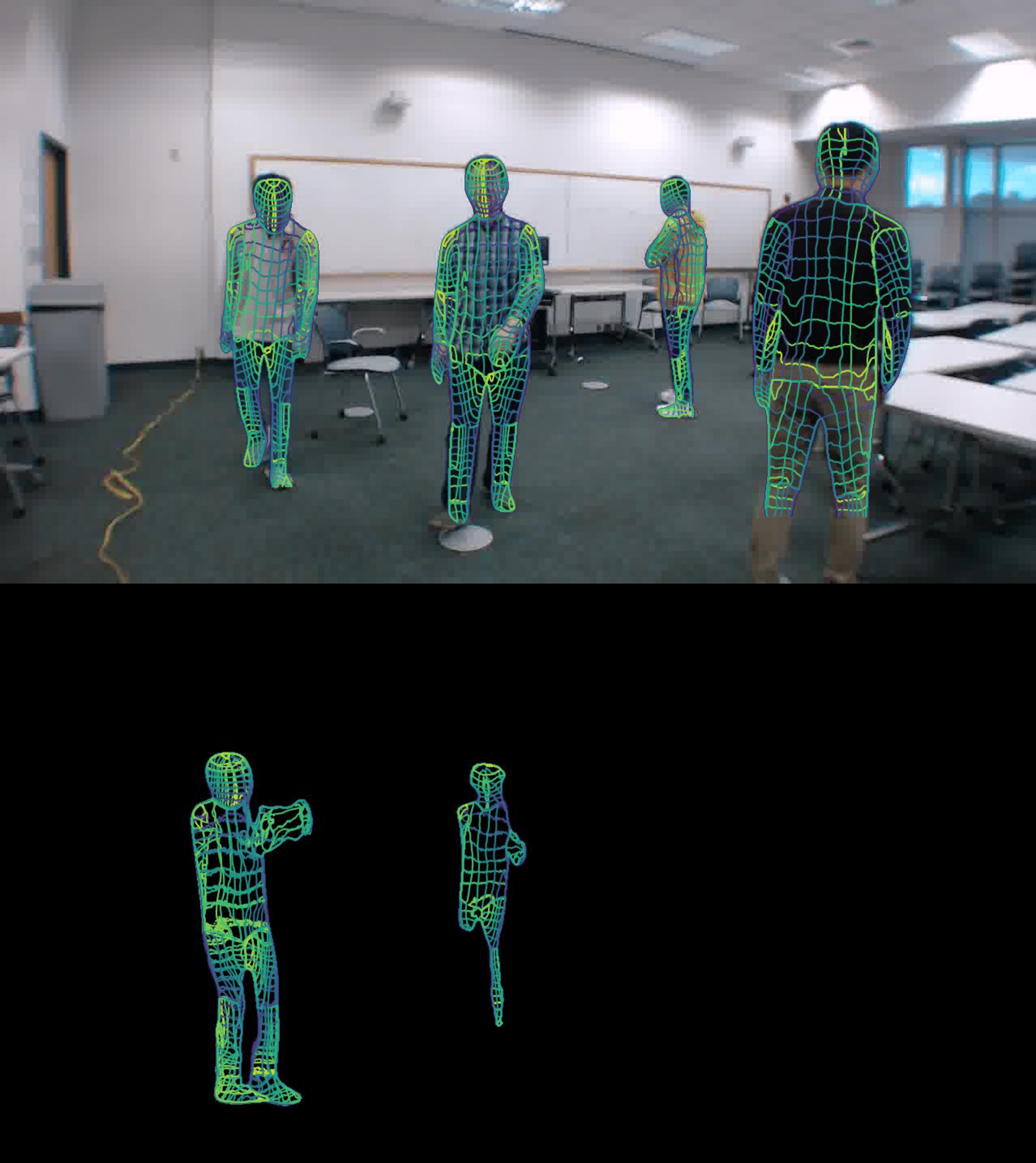
(c)

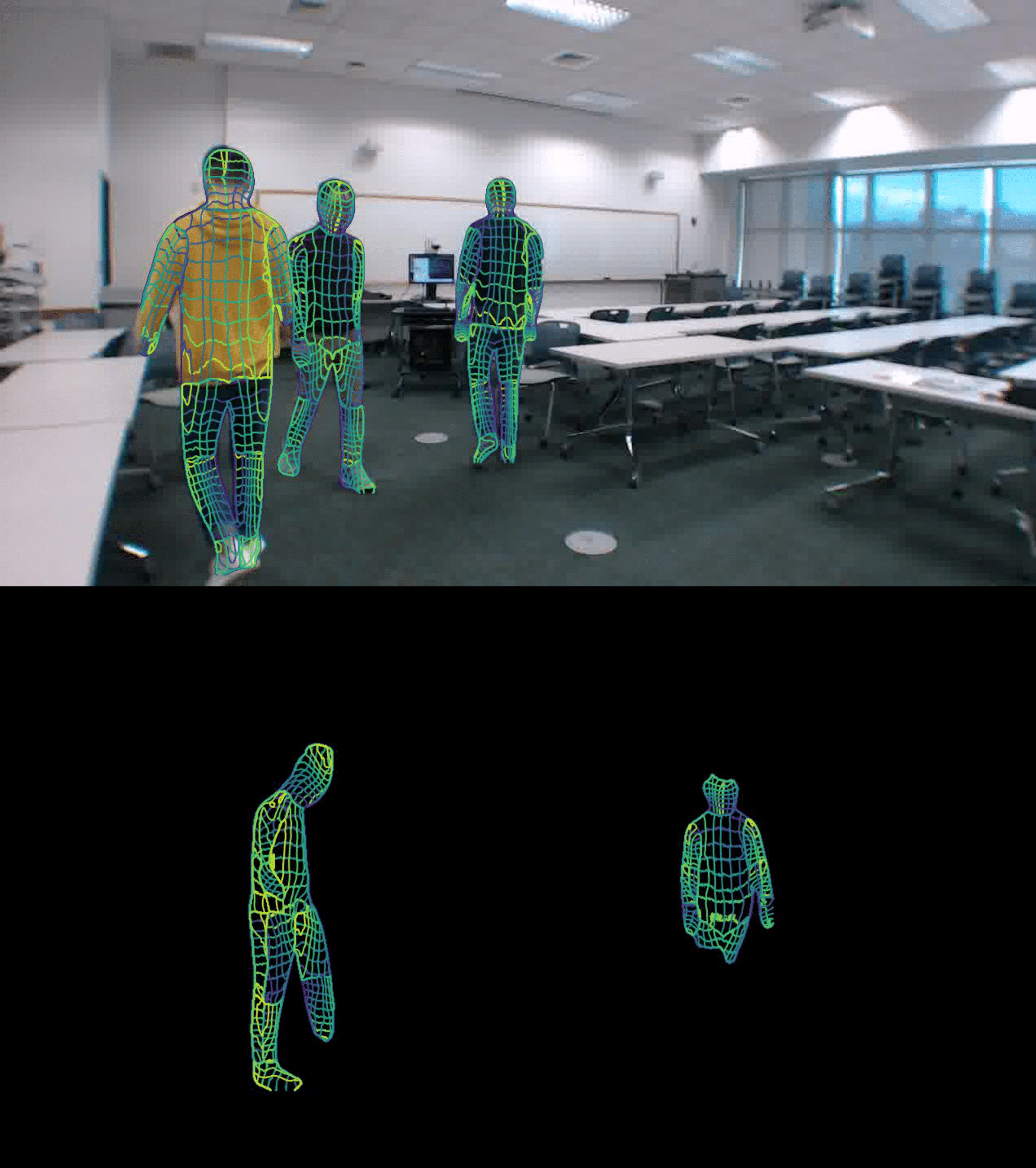
(d)

Figure 8. Examples pf failure cases: (a-b) rare poses; (c-d) Three or more concurrent subjects. The first row is ground truth dense pose estimation. The second row illustrates the predicted dense pose.

All above results are obtained using the same layout for training and testing. However, WiFi signals in different environments exhibit significantly different propagation patterns. Therefore, it is still a very challenging problem to deploy our model on data from an untrained layout.

To test the robustness of our model, we conducted the previous experiment under the different layout protocols, where there are 15 training layouts and 1 testing layout. The experimental results are recorded in Table 7 and Table 8.

We can observe that our final model performs better than the baseline model in the unseen domain, but the performance decreases significantly from that under the same layout protocol: the AP performance drops from $43.5$ to $27.3$ and dpAP$\cdot$GPS drops from $45.3$ to $25.4$. However, it should also be noted that the image-based model suffers from the same domain generalization problem. We believe a more comprehensive dataset from a wide range of settings can alleviate this issue.

Figure 9. Qualitative comparison using synchronized images and WiFi signals. (Left Column) image-based DensePose (Right Column) our WiFi-based DensePose.

4.8. Failure cases

We observed two main types of failure cases. (1) When there are body poses that rarely occurred in the training set, the WiFi-based model is biased and is likely to produce wrong body parts (See examples (a-b) in Figure 8). (2) When there are three or more concurrent subjects in one capture, it is more challenging for the WiFi-based model to extract detailed information for each individual from the amplitude and phase tensors of the entire capture. (See examples (c-d) in Figure 8). We believe both of these issues can be resolved by obtaining more comprehensive training data.

5. Conclusion and future work

In this paper, we demonstrated that it is possible to obtain dense human body poses from WiFi signals by utilizing deep learning architectures commonly used in computer vision. Instead of directly training a randomly initialized WiFi-based model, we explored rich supervision information to improve both the performance and training efficiency, such as utilizing the CSI phase, adding keypoint detection branch, and transfer learning from an image-based model. The performance of our work is still limited by the public training data in the field of WiFi-based perception, especially under different layouts. In future work, we also plan to collect multi-layout data and extend our work to predict 3D human body shapes from WiFi signals. We believe that the advanced capability of dense perception could empower the WiFi device as a privacy-friendly, illumination-invariant, and cheap human sensor compared to RGB cameras and Lidars.

References

- (1)
- Adib et al. (2015) Fadel Adib, Chen-Yu Hsu, Hongzi Mao, Dina Katabi, and Frédo Durand. 2015. Capturing the Human Figure through a Wall. ACM Trans. Graph. 34, 6, Article 219 (oct 2015), 13 pages. https://doi.org/10.1145/2816795.2818072
- Adib et al. (2014) Fadel Adib, Zach Kabelac, Dina Katabi, and Robert C. Miller. 2014. 3D Tracking via Body Radio Reflections. In 11th USENIX Symposium on Networked Systems Design and Implementation (NSDI 14). USENIX Association, Seattle, WA, 317–329. https://www.usenix.org/conference/nsdi14/technical-sessions/presentation/adib
- Alldieck et al. (2019) Thiemo Alldieck, Gerard Pons-Moll, Christian Theobalt, and Marcus Magnor. 2019. Tex2Shape: Detailed Full Human Body Geometry From a Single Image. arXiv:1904.08645 [cs.CV]
- Andriluka et al. (2018) Mykhaylo Andriluka, Umar Iqbal, Eldar Insafutdinov, Leonid Pishchulin, Anton Milan, Juergen Gall, and Bernt Schiele. 2018. PoseTrack: A Benchmark for Human Pose Estimation and Tracking. arXiv:1710.10000 [cs.CV]
- BASRI and Khadimi (2016) Chaimaa BASRI and Ahmed El Khadimi. 2016. Survey on indoor localization system and recent advances of WIFI fingerprinting technique. In International Conference on Multimedia Computing and Systems.
- Bristow et al. (2015) Hilton Bristow, Jack Valmadre, and Simon Lucey. 2015. Dense Semantic Correspondence where Every Pixel is a Classifier. arXiv:1505.04143 [cs.CV]
- Cao et al. (2019) Zhe Cao, Gines Hidalgo, Tomas Simon, Shih-En Wei, and Yaser Sheikh. 2019. OpenPose: Realtime Multi-Person 2D Pose Estimation using Part Affinity Fields. arXiv:1812.08008 [cs.CV]
- Güler et al. (2018) Riza Alp Güler, Natalia Neverova, and Iasonas Kokkinos. 2018. DensePose: Dense Human Pose Estimation In The Wild. CoRR abs/1802.00434 (2018). arXiv:1802.00434 http://arxiv.org/abs/1802.00434
- He et al. (2017) Kaiming He, Georgia Gkioxari, Piotr Dollár, and Ross B. Girshick. 2017. Mask R-CNN. CoRR abs/1703.06870 (2017). arXiv:1703.06870 http://arxiv.org/abs/1703.06870
- Jiang et al. (2017) Weipeng Jiang, Yongjun Liu, Yun Lei, Kaiyao Wang, Hui Yang, and Zhihao Xing. 2017. For Better CSI Fingerprinting Based Localization: A Novel Phase Sanitization Method and a Distance Metric. In 2017 IEEE 85th Vehicular Technology Conference (VTC Spring). 1–7. https://doi.org/10.1109/VTCSpring.2017.8108351
- Kefayati et al. (2020) Mohammad Hadi Kefayati, Vahid Pourahmadi, and Hassan Aghaeinia. 2020. Wi2Vi: Generating Video Frames from WiFi CSI Samples. CoRR abs/2001.05842 (2020). arXiv:2001.05842 https://arxiv.org/abs/2001.05842
- Kocabas et al. (2020) Muhammed Kocabas, Nikos Athanasiou, and Michael J. Black. 2020. VIBE: Video Inference for Human Body Pose and Shape Estimation. arXiv:1912.05656 [cs.CV]
- Ledergerber and D’Andrea (2019) Anton Ledergerber and Raffaello D’Andrea. 2019. Ultra-Wideband Angle of Arrival Estimation Based on Angle-Dependent Antenna Transfer Function. Sensors 19, 20 (2019). https://doi.org/10.3390/s19204466
- Lin et al. (2016) Tsung-Yi Lin, Piotr Dollár, Ross B. Girshick, Kaiming He, Bharath Hariharan, and Serge J. Belongie. 2016. Feature Pyramid Networks for Object Detection. CoRR abs/1612.03144 (2016). arXiv:1612.03144 http://arxiv.org/abs/1612.03144
- Lin et al. (2014) Tsung-Yi Lin, Michael Maire, Serge J. Belongie, Lubomir D. Bourdev, Ross B. Girshick, James Hays, Pietro Perona, Deva Ramanan, Piotr Dollár, and C. Lawrence Zitnick. 2014. Microsoft COCO: Common Objects in Context. CoRR abs/1405.0312 (2014). arXiv:1405.0312 http://arxiv.org/abs/1405.0312
- Long et al. (2014) Jonathan Long, Evan Shelhamer, and Trevor Darrell. 2014. Fully Convolutional Networks for Semantic Segmentation. CoRR abs/1411.4038 (2014). arXiv:1411.4038 http://arxiv.org/abs/1411.4038
- Maturana and Scherer (2015) Daniel Maturana and Sebastian Scherer. 2015. VoxNet: A 3D Convolutional Neural Network for real-time object recognition. In 2015 IEEE/RSJ International Conference on Intelligent Robots and Systems (IROS). 922–928. https://doi.org/10.1109/IROS.2015.7353481
- Neverova et al. (2020) Natalia Neverova, David Novotny, Vasil Khalidov, Marc Szafraniec, Patrick Labatut, and Andrea Vedaldi. 2020. Continuous Surface Embeddings. Advances in Neural Information Processing Systems.
- Redmon and Farhadi (2018) Joseph Redmon and Ali Farhadi. 2018. YOLOv3: An Incremental Improvement. arXiv:1804.02767 [cs.CV]
- Ren et al. (2015a) Shaoqing Ren, Kaiming He, Ross B. Girshick, and Jian Sun. 2015a. Faster R-CNN: Towards Real-Time Object Detection with Region Proposal Networks. CoRR abs/1506.01497 (2015). arXiv:1506.01497 http://arxiv.org/abs/1506.01497
- Ren et al. (2015b) Shaoqing Ren, Kaiming He, Ross B. Girshick, and Jian Sun. 2015b. Faster R-CNN: Towards Real-Time Object Detection with Region Proposal Networks. CoRR abs/1506.01497 (2015). arXiv:1506.01497 http://arxiv.org/abs/1506.01497
- Saito et al. (2019) Shunsuke Saito, , Zeng Huang, Ryota Natsume, Shigeo Morishima, Angjoo Kanazawa, and Hao Li. 2019. PIFu: Pixel-Aligned Implicit Function for High-Resolution Clothed Human Digitization. arXiv preprint arXiv:1905.05172 (2019).
- Sen et al. (2012) Souvik Sen, Božidar Radunovic, Romit Roy Choudhury, and Tom Minka. 2012. You Are Facing the Mona Lisa: Spot Localization Using PHY Layer Information. In Proceedings of the 10th International Conference on Mobile Systems, Applications, and Services (Low Wood Bay, Lake District, UK) (MobiSys ’12). Association for Computing Machinery, New York, NY, USA, 183–196. https://doi.org/10.1145/2307636.2307654
- Shapovalov et al. (2021) Roman Shapovalov, David Novotný, Benjamin Graham, Patrick Labatut, and Andrea Vedaldi. 2021. DensePose 3D: Lifting Canonical Surface Maps of Articulated Objects to the Third Dimension. CoRR abs/2109.00033 (2021). arXiv:2109.00033 https://arxiv.org/abs/2109.00033
- Sheng et al. (2020) B. Sheng, F. Xiao, L. Sha, and L. Sun. 2020. Deep Spatial–Temporal Model Based Cross-Scene Action Recognition Using Commodity WiFi. IEEE Internet of Things Journal 7 (2020).
- Soltanaghaei et al. (2018a) Elahe Soltanaghaei, Avinash Kalyanaraman, and Kamin Whitehouse. 2018a. Multipath Triangulation: Decimeter-Level WiFi Localization and Orientation with a Single Unaided Receiver. In Proceedings of the 16th Annual International Conference on Mobile Systems, Applications, and Services (Munich, Germany) (MobiSys ’18). Association for Computing Machinery, New York, NY, USA, 376–388. https://doi.org/10.1145/3210240.3210347
- Soltanaghaei et al. (2018b) Elahe Soltanaghaei, Avinash Kalyanaraman, and Kamin Whitehouse. 2018b. Multipath Triangulation: Decimeter-level WiFi Localization and Orientation with a Single Unaided Receiver. In Proceedings of the 16th Annual International Conference on Mobile Systems, Applications, and Services.
- Sun et al. (2021) Yu Sun, Qian Bao, Wu Liu, Yili Fu, Michael J. Black, and Tao Mei. 2021. Monocular, One-stage, Regression of Multiple 3D People. arXiv:2008.12272 [cs.CV]
- Wang et al. (2019a) Fei Wang, Yunpeng Song, Jimuyang Zhang, Jinsong Han, and Dong Huang. 2019a. Temporal Unet: Sample Level Human Action Recognition using WiFi. arXiv Preprint arXiv:1904.11953 (2019).
- Wang et al. (2019b) Fei Wang, Sanping Zhou, Stanislav Panev, Jinsong Han, and Dong Huang. 2019b. Person-in-WiFi: Fine-grained Person Perception using WiFi. CoRR abs/1904.00276 (2019). arXiv:1904.00276 http://arxiv.org/abs/1904.00276
- Wang et al. (2019c) Fei Wang, Sanping Zhou, Stanislav Panev, Jinsong Han, and Dong Huang. 2019c. Person-in-WiFi: Fine-grained Person Perception using WiFi. In ICCV.
- Wang et al. (2018) Zhe Wang, Yang Liu, Qinghai Liao, Haoyang Ye, Ming Liu, and Lujia Wang. 2018. Characterization of a RS-LiDAR for 3D Perception. In 2018 IEEE 8th Annual International Conference on CYBER Technology in Automation, Control, and Intelligent Systems (CYBER). 564–569. https://doi.org/10.1109/CYBER.2018.8688235
- Wei et al. (2016) Shih-En Wei, Varun Ramakrishna, Takeo Kanade, and Yaser Sheikh. 2016. Convolutional Pose Machines. arXiv:1602.00134 [cs.CV]
- Xiao et al. (2018) Bin Xiao, Haiping Wu, and Yichen Wei. 2018. Simple Baselines for Human Pose Estimation and Tracking. arXiv:1804.06208 [cs.CV]
- Xu et al. (2019) Yuanlu Xu, Song-Chun Zhu, and Tony Tung. 2019. DenseRaC: Joint 3D Pose and Shape Estimation by Dense Render-and-Compare. CoRR abs/1910.00116 (2019). arXiv:1910.00116 http://arxiv.org/abs/1910.00116
- Xue et al. (2021) Hongfei Xue, Yan Ju, Chenglin Miao, Yijiang Wang, Shiyang Wang, Aidong Zhang, and Lu Su. 2021. mmMesh: towards 3D real-time dynamic human mesh construction using millimeter-wave. In Proceedings of the 19th Annual International Conference on Mobile Systems, Applications, and Services. 269–282.
- Yao et al. (2019) Pengfei Yao, Zheng Fang, Fan Wu, Yao Feng, and Jiwei Li. 2019. DenseBody: Directly Regressing Dense 3D Human Pose and Shape From a Single Color Image. arXiv:1903.10153 [cs.CV]
- Zhang et al. (2020) Hongwen Zhang, Jie Cao, Guo Lu, Wanli Ouyang, and Zhenan Sun. 2020. Learning 3D Human Shape and Pose from Dense Body Parts. arXiv:1912.13344 [cs.CV]
- Zhao et al. (2018) Mingmin Zhao, Tianhong Li, Mohammad Abu Alsheikh, Yonglong Tian, Hang Zhao, Antonio Torralba, and Dina Katabi. 2018. Through-Wall Human Pose Estimation Using Radio Signals. In 2018 IEEE/CVF Conference on Computer Vision and Pattern Recognition. 7356–7365. https://doi.org/10.1109/CVPR.2018.00768
- Zhou et al. (2016) Tinghui Zhou, Philipp Krähenbühl, Mathieu Aubry, Qixing Huang, and Alexei A. Efros. 2016. Learning Dense Correspondence via 3D-guided Cycle Consistency. arXiv:1604.05383 [cs.CV]