Bounds on heat transport for two-dimensional buoyancy driven flows between rough boundaries

Abstract

We consider the two-dimensional Rayleigh-Bénard convection in a layer of fluid between rough Navier-slip boundaries. The top and bottom boundaries are described by the same height function $h$. We prove rigorous upper bounds on the Nusselt number which capture the dependence on the curvature of the boundary $\kappa$ and the (non-constant) friction coefficient $\alpha$ explicitly. For $h\in W^{2,\infty}$ and $\kappa$ satisfying a smallness condition with respect to $\alpha$, we find

$${\rm{Nu}}\lesssim{\rm{Ra}}^{\frac{1}{2}}+\|\kappa\|_{\infty}\,,$$

which agrees with the predicted Spiegel-Kraichnan scaling when $\kappa=0$. This bound is obtained via local regularity estimates in a small strip at the boundary. When $h\in W^{3,\infty}$ and the functions $\kappa$ and $\alpha$ are sufficiently small in $L^{\infty}$, we prove upper bounds using the background field method, which interpolate between ${\rm{Ra}}^{\frac{1}{2}}$ and ${\rm{Ra}}^{\frac{5}{12}}$ with non-trivial dependence on $\alpha$ and $\kappa$. These bounds agree with the result in [DNN22] for flat boundaries and constant friction coefficient. Furthermore, in the regime $\Pr\geq{\rm{Ra}}^{\frac{5}{7}}$, we improve the ${\rm{Ra}}^{\frac{1}{2}}$-upper bound, showing

$${\rm{Nu}}\lesssim_{\alpha,\kappa}{\rm{Ra}}^{\frac{3}{7}}\,,$$

where $\lesssim_{\alpha,\kappa}$ hides an additional dependency of the implicit constant on $\alpha$ and $\kappa$.

Keywords: Rayleigh-Bénard convection, Navier-slip boundary conditions, rough boundaries, scaling laws, upper bounds

1 Introduction

In this paper we deal with the Rayleigh-Bénard convection problem, modelled by the Boussinesq system for the velocity field $u=(u_{1},u_{2})\in{\mathbb{R}}^{2}$, the scalar temperature field $T$ and the pressure $p$

$$\frac{1}{\rm{Pr}}(u_{t}+u\cdot\nabla u)-\Delta u+\nabla p ={\rm{Ra}}Te_{2}$$ (NS)

$$\nabla\cdot u =0$$ (DF)

$$T_{t}+u\cdot\nabla T-\Delta T =0$$ (AD)

set in the regular and bounded domain

$$\Omega=\{(y_{1},y_{2})\in\mathbb{R}^{2}\ |\ 0<y_{1}<\Gamma,h(y_{1})<y_{2}<1+h(y_{1})\}$$

where $h$ describes the height of the bottom boundary and $e_{2}=(0,1)$. The nondimensional numbers ${\rm{Ra}}$ and $\Pr$ are the Rayleigh and Prandtl number respectively. We assume periodicity of all variables in the $e_{1}=(1,0)$-direction and impose

$$T =1 \textnormal{ on }\gamma^{-}$$ (1)

$$T =0 \textnormal{ on }\gamma^{+}$$

where $\gamma^{-}=\{(y_{1},y_{2})\in\mathbb{R}^{2}\ |\ 0<y_{1}<\Gamma,y_{2}=h(y_{1})\}$ and $\gamma^{+}=\{(y_{1},y_{2})\in\mathbb{R}^{2}\ |\ 0<y_{1}<\Gamma,y_{2}=1+h(y_{1})\}$ are the bottom and top boundary respectively. Our goal is to derive physically meaningful upper bounds for the Nusselt number, a quantity that measures the average heat transport in the vertical direction. In the last thirty years, the problem of deriving scaling laws for the Nusselt number in turbulent convection between two horizontal plates has been highly investigated both in experiments and numerical studies (cf.[AGL09] and references therein). Our analysis wants to capture the role of geometry and boundary conditions in the scaling laws for the Nusselt number.

Intentionally, we did not yet specify the boundary conditions for $u$ at $\gamma^{+}$ and $\gamma^{-}$. Before doing that, we recall some important results under no-slip and free-slip boundary conditions, which are the most studied for this problem. The no-slip boundary conditions in the case of flat boundaries (i.e. $h=0$) read

$$u=0\quad\mbox{ at }\quad y_{2}=\{0,1\}\,.$$

In this setting, Doering and Constantin in 1996 [DC96] rigorously proved the upper bound ${\rm{Nu}}\lesssim{\rm{Ra}}^{\frac{1}{2}}$ in three-dimensions. From this seminal result, many works followed aiming at optimizing the ${\rm{Ra}}^{\frac{1}{2}}$-upper bound (see [Nob23], [FAW22] and references therein). In the infinite-Prandtl number setting, a series of works [CD99], [DOR06], [OS11] established the bound ${\rm{Nu}}\lesssim{\rm{Ra}}^{\frac{1}{3}}$ up to a logarithmic correction. A lower bound within the method proposed in [CD99] was proved in [NO17]. In the finite Prandtl number case, Choffrut, Otto and the second author of this paper in [CNO16] improved the perturbative result of Wang [Wan08] showing ${\rm{Nu}}\lesssim({\rm{Ra}}\ln{\rm{Ra}})^{\frac{1}{3}}$ for $\rm{Pr}\gtrsim({\rm{Ra}}\ln{\rm{Ra}})^{\frac{1}{3}}$ and the crossover to the bound ${\rm{Nu}}\lesssim(\Pr^{-1}{\rm{Ra}}\ln{\rm{Ra}})^{\frac{1}{2}}$ for $\rm{Pr}\lesssim({\rm{Ra}}\ln{\rm{Ra}})^{\frac{1}{3}}$. The methods proposed by Doering and Constantin in the nineties to produce scaling laws for the Nusselt number in boundary-driven convection continues to be fruitfully employed in other (related) problems [Tob22],[DC01],[FNW20], [Ars+21] (see also [Gol16] and references therein). Recently, remarkable results have been produced concerning the saturation of the upper bounds [DT19],[Kum22]. The question around the ”ultimate scaling law” in the Rayleigh-Bénard convection problem was recently object of animated discussions [DTW19] and it remains unclear whether at large Rayleigh number the scaling ${\rm{Nu}}\sim{\rm{Ra}}^{\frac{1}{2}}$ will prevail over the scaling ${\rm{Nu}}\sim{\rm{Ra}}^{\frac{1}{3}}$ or whether another scaling arises.

The no-slip boundary conditions are the most used in theoretical and numerical studies, but whether or not they represent the most ”realistic” conditions, is subject to debate (see [Nob23] and references therein). In 2011 Doering and Whitehead [WD11] remarkably proved ${\rm{Nu}}\lesssim{\rm{Ra}}^{\frac{5}{12}}$ in the two-dimensional Rayleigh-Bénard convection problem between flat horizontal boundaries, with free-slip boundary conditions, i.e.

$$u_{2}=0\quad\mbox{ and }\quad\partial_{2}u_{1}=0\quad\mbox{ at }\quad y_{2}=\{0,1\}\,.$$

This result rules out the ${\rm{Nu}}\sim{\rm{Ra}}^{\frac{1}{2}}$ scaling in this setting. But the question about the optimality of this upper bound remains along with the question whether the scaling ${\rm{Nu}}\sim{\rm{Ra}}^{\frac{5}{12}}$ carries a physical meaning. Motivated by this result, in [DNN22] Drivas, Nguyen and the second author of this paper considered the two-dimensional Rayleigh-Bénard convection problem with the following conditions on the horizontal plates:

$$u_{2}=0\quad\mbox{ and }\quad\partial_{2}u_{1}=\frac{1}{L_{s}}u_{1}\quad\mbox{ at }\quad y_{2}=\{0,1\}\,,$$ (2)

where $L_{s}$ is the (constant) ”slip-length”. Under these assumptions the authors proved the interpolation bound

$${\rm{Nu}}\lesssim{\rm{Ra}}^{\frac{5}{12}}+\frac{1}{L_{s}^{2}}{\rm{Ra}}^{\frac{1}{2}}\qquad\mbox{ in the regime }\qquad\Pr\gtrsim\frac{1}{L_{s}^{2}}{\rm{Ra}}^{\frac{3}{4}}\,.$$

Relatively few theoretical works have addressed the problem of the Nusselt number scaling in the case of rough boundaries in Rayleigh-Bénard convection: In [SW11] Shishkina and Wagner developed an analytical model to estimate the Nusselt number deviations caused by the wall roughness and in [WS15] the same authors performed direct numerical simulations. In [GD16] Goluskin and Doering considered the three-dimensional Rayleigh-Bénard problem between rough boundaries. In particular, under the assumption that the profile $h$ (which may differ at the top and bottom boundaries) is a continuous and piecewise differentiable function of the horizontal coordinates and has squared-integrable gradients, the authors showed ${\rm{Nu}}\lesssim C(\|\nabla h\|_{2}^{2}){\rm{Ra}}^{\frac{1}{2}}$. Here we want to cite also [Ker16] and [Ker18], where Kerswell derives an upper bound for the energy dissipation rate per unit mass for a pressure-driven flow in a rough channel.

The boundary conditions in (2) are the simplified version of the original Navier-slip boundary conditions [Nav23]

$$\tau\cdot\mathbb{D}u\cdot n+\alpha u_{\tau} =0 \textnormal{ on }\gamma^{+}\cup\gamma^{-}$$ (3)

$$u\cdot n =0 \textnormal{ on }\gamma^{+}\cup\gamma^{-},$$

Here we denoted with $n$ and $\tau$ the outward unit normal and tangential vector to the boundary respectively, with $u_{\tau}=u\cdot\tau$ the tangential velocity and with $\mathbb{D}u_{ij}=\frac{1}{2}(\partial_{i}u_{j}+\partial_{j}u_{i})$ the strain tensor. The space-dependent function $\alpha\geq 0$ is the friction coefficient and measures the tendency of the fluid to slip on the boundary. It may vary along $\gamma^{-}$ and $\gamma^{+}$. The problem is illustrated in Figure 1. We notice that the Navier-slip boundary conditions have been studied in a variety of problems in fluid mechanics. They have been considered in problems related to mixing [HW18] as well as rotating systems [DG17]. In [AEG21] and [Ace+19] the authors studied the Stokes operator with Navier-slip boundary conditions and the convergence to no-slip boundary conditions as $\alpha\to\infty$.

In this paper we want to generalize the result in [DNN22], considering the original Navier-slip boundary conditions (3), hence allowing a non-constant (space dependent) friction coefficient. Furthermore, we allow a certain degree of roughness at the upper and lower plates.

Our first, more general result is the following

Theorem 1.1.

Let $u$ and $T$ solve system (NS)-(DF)-(AD), with boundary conditions (1) and (3). Assume $h\in W^{2,\infty}[0,\Gamma]$, $\alpha>0$ and $\kappa$ satisfies

$$|\kappa|\leq 2\alpha+\frac{1}{4\sqrt{1+(h^{\prime})^{2}}}\min\left\{1,\sqrt{\alpha}\right\}$$ (4)

pointwise almost everywhere on $\gamma^{-}\cup\gamma^{+}$. Then there exists a constant $C>0$ depending only on $\|h^{\prime}\|_{\infty}$ and $|\Omega|$ such that

$${\rm{Nu}}\leq C{\rm{Ra}}^{\frac{1}{2}}+C\|\kappa\|_{\infty}$$ (5)

for all ${\rm{Ra}}\geq 1$.

This upper bound catches the classical Kraichnan-Spiegel scaling ${\rm{Ra}}^{\frac{1}{2}}$ and is uniform in the Prandtl number. The novelty of this (expected) result is to show explicitly the role played by the functions $\alpha$ and $\kappa$ in the bound. We notice that the bound holds under assumption (4) which relates the magnitude of $|\kappa|$ and $\alpha$. Since $\kappa$ changes sign, this assumption is crucial to obtain the energy decay estimate (see Lemma 3.3). As we can see from (5), the bound deteriorates as roughness (quantified by $\|\kappa\|_{\infty}$) increases.

Under more restrictive regularity assumptions on the height-function, we can prove the following

Theorem 1.2.

Let $u$ and $T$ solve the system (NS)-(DF)-(AD), with boundary conditions (1) and (3). Let $h\in W^{3,\infty}[0,\Gamma]$, $\alpha\in W^{1,\infty}(\gamma^{-}\cup\gamma^{+})$ and $u_{0}\in W^{1,r}(\Omega)$ for some $r>2$. Set $\underline{\alpha}:=\min_{\gamma^{-}\cup\gamma^{+}}\alpha>0$. Then there exists a constant $0<\bar{C}<1$ such that for all $\alpha$ and $\kappa$ with

$$\|\alpha+\kappa\|_{\infty}\leq\bar{C}$$ (6)

the following bounds on the Nusselt number hold:

1. If $|\kappa|\leq\alpha$ on $\gamma^{-}\cup\gamma^{+}$, $\rm{Pr}\geq\underline{\alpha}^{-\frac{3}{2}}{\rm{Ra}}^{\frac{3}{4}}$ and ${\rm{Ra}}^{-\frac{1}{2}}\leq\underline{\alpha}$ then

   $${\rm{Nu}}\leq C_{\frac{1}{2}}\|\alpha+\kappa\|_{W^{1,\infty}}^{2}{\rm{Ra}}^{\frac{1}{2}}+C_{\frac{5}{12}}{\rm{Ra}}^{\frac{5}{12}}.$$ (7)

2. If $|\kappa|\leq 2\alpha+\frac{1}{4\sqrt{1+(h^{\prime})^{2}}}\sqrt{\alpha}$ on $\gamma^{-}\cup\gamma^{+}$, $\rm{Pr}\geq\underline{\alpha}^{-\frac{3}{2}}{\rm{Ra}}^{\frac{3}{4}}$ and ${\rm{Ra}}^{-1}\leq\underline{\alpha}$ then

   $${\rm{Nu}}\leq C_{\frac{1}{2}}\sqrt{\underline{\alpha}}\|\alpha+\kappa\|_{W^{1,\infty}}^{2}{\rm{Ra}}^{\frac{1}{2}}+C_{\frac{5}{12}}\underline{\alpha}^{-\frac{1}{12}}{\rm{Ra}}^{\frac{5}{12}}.$$ (8)

3. If $|\kappa|\leq 2\alpha+\frac{1}{4\sqrt{1+(h^{\prime})^{2}}}\sqrt{\alpha}$ on $\gamma^{-}\cup\gamma^{+}$ and $\rm{Pr}\geq{\rm{Ra}}^{\frac{5}{7}}$ then

   $${\rm{Nu}}\leq C_{\frac{3}{7}}{\rm{Ra}}^{\frac{3}{7}}.$$ (9)

The constants are given by

$$C_{\frac{1}{2}} =C(1+\|u_{0}\|_{W^{1,r}}^{2})^{-1}$$

$$C_{\frac{5}{12}} =C\left(\|u_{0}\|_{W^{1,r}}+\|\dot{\alpha}\|_{\infty}+\|\dot{\kappa}\|_{\infty}+1\right)^{\frac{1}{3}}$$

$$C_{\frac{3}{7}} =C\left(\|\alpha+\kappa\|_{W^{1,\infty}}^{2}+\underline{\alpha}^{-\frac{1}{2}}+\underline{\alpha}^{-\frac{1}{6}}(\|u_{0}\|_{W^{1,r}}+\|\dot{\alpha}\|_{\infty}+\|\dot{\kappa}\|_{\infty}+1)^{\frac{1}{3}}\right),$$

where $\dot{\alpha}$ and $\dot{\kappa}$ are the derivatives of $\alpha$ and $\kappa$ along the boundary and $C>0$ denotes a constant depending only on the size of the domain $|\Omega|$, $\|h^{\prime}\|_{\infty}$ and $r$.

First of all, we notice that our results in Theorem 1.1 and Theorem 1.2 also cover the case of flat-boundaries and generic friction coefficient $\alpha$. In fact, all results (i.e. (5), (7), (8) and (9)) hold setting $\kappa=0$.

We observe that Theorem 1.2 only holds under the smallness assumption (6), while there is no such restriction in Theorem 1.1. If $\kappa$ and $\alpha$ are big, and related through (4), then the bound (5) holds. Additionally, note that Theorem 1.2 requires the rather restrictive assumption $h\in W^{3,\infty}$ to ensure $\kappa\in W^{1,\infty}$.

The interpolation bound (7) coincides with the result in [DNN22], when $\kappa=0$ and $\alpha=\frac{1}{L_{s}}$. The main advantage of the interpolation results (7) and (8) is in the regime of small $\|\alpha\|_{W^{1,\infty}}$ and $\|\kappa\|_{W^{1,\infty}}$. In fact, notice that if $\kappa\sim{\rm{Ra}}^{-\nu}$ and $\alpha\sim{\rm{Ra}}^{-\mu}$, then (7) translates into

$${\rm{Nu}}\lesssim\begin{cases}{\rm{Ra}}^{-2\mu+\frac{1}{2}}&\mbox{ if }\mu<\frac{1}{24}\\ {\rm{Ra}}^{\frac{5}{12}}&\mbox{ if }\frac{1}{24}\leq\mu<\frac{1}{2}\end{cases}$$

and $\nu\geq\mu$. This means that the best bound is achieved in the case $\frac{1}{24}\leq\mu<\frac{1}{2}$ and $\Pr\gtrsim{\rm{Ra}}^{\frac{3}{2}\mu+\frac{3}{4}}$. Notice that, while (7) holds only under the assumption $|\kappa|\leq\alpha$, the upper bound (8) holds under the weaker assumption $|\kappa|\leq 2\alpha+\frac{1}{4\sqrt{1+(h^{\prime})^{2}}}\sqrt{\alpha}$ on $\gamma^{-}\cup\gamma^{+}$, allowing $|\kappa|>\alpha$ especially when $\alpha$ and $|\kappa|$ are very small. We observe that in the regime of small $\alpha$ and $\kappa$, say $\|\alpha\|_{W^{1,\infty}},\|\kappa\|_{W^{1,\infty}}\leq 1$, the constant $C_{\frac{5}{12}}$ becomes independent of $\alpha$ and $\kappa$. Finally we remark that if the condition ${\rm{Ra}}^{-1}\leq\underline{\alpha}$ for (8) is violated, then (5) yields a stricter bound.

Interestingly (9) improves the upper bound (5) in the case of small $\|\alpha+\kappa\|_{\infty}$ and big $\rm{Pr}$, i.e. $\rm{Pr}\geq{\rm{Ra}}^{\frac{5}{7}}$. While the interpolation bound (7) yields a better result if $\alpha\sim{\rm{Ra}}^{-\mu}$, (9) provides the sharpest bound if $\alpha$ and $\kappa$ are independent of ${\rm{Ra}}$. Notice that, differently from the constant prefactor in (5), the constant $C_{\frac{3}{7}}$ also depends on $\alpha$ and $\kappa$.

2 Preliminaries

We start with introducing some notation and facts we will use in the whole paper. We will often use that the tangential vector to the boundary $\tau$ can be written as $\tau=n^{\perp}=(-n_{2},n_{1})$, where $n$ is outward unit normal and $u_{\tau}=u\cdot\tau$. The curvature of the boundaries $\kappa$ is given by $\frac{d}{d\lambda}\tau=\kappa n$, where $\lambda$ is the parameterization of the boundaries by arc length in $\tau$-direction. The problem is illustrated in Figure 1.

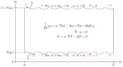
Figure 1: Illustration of the Rayleigh-Bénard convection problem with Navier-slip boundary conditions and rough boundaries considered in this paper: (NS), (DF), (AD), (1),(3).

We will use the following notation to denote space-time averages

$$\langle f\rangle =\limsup_{t\to\infty}\frac{1}{t}\int_{0}^{t}\frac{1}{|\Omega|}\int_{\Omega}f\ dy\ dt,$$

$$\langle f\rangle_{\gamma^{-}} =\limsup_{t\to\infty}\frac{1}{t}\int_{0}^{t}\frac{1}{|\Omega|}\int_{\gamma^{-}}f\ dS\ dt,$$

$$\langle f\rangle_{\gamma^{-}\cup\gamma^{+}} =\limsup_{t\to\infty}\frac{1}{t}\int_{0}^{t}\frac{1}{|\Omega|}\int_{\gamma^{-}\cup\gamma^{+}}f\ dS\ dt.$$

Moreover, on the set

$$\gamma(x_{2})=\left\{(y_{1},y_{2})\ \middle|\ 0<y_{1}<\Gamma,y_{2}=h(y_{1})+x_{2}\right\},$$ (10)

where $0\leq x_{2}\leq 1$, illustrated in Figure 2, we define the average

$$\langle f\rangle_{\gamma(x_{2})} =\limsup_{t\to\infty}\frac{1}{t}\int_{0}^{t}\frac{1}{|\Omega|}\int_{\gamma(x_{2})}f\ dS\,dt.$$

In what follows we will consider $0\leq T_{0}\leq 1$, implying

$$\|T\|_{\infty}\leq 1$$ (11)

for all times $t>0$, by the maximum principle for the temperature.

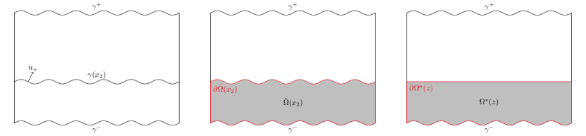
Figure 2: Illustrations of $\gamma(x_{2})$, $\tilde{\Omega}(x_{2})$ and $\Omega^{\star}(z)$

Next we define the Nusselt number.

Definition 2.1.

The Nusselt number is defined as

$${\rm{Nu}}=\langle|\nabla T|^{2}\rangle.$$ (12)

It also admits other equivalent representations, as stated in the following.

Proposition 2.1.

The Nusselt number satisfies

$${\rm{Nu}}={} \langle n\cdot\nabla T\rangle_{\gamma^{-}}$$ (13)

$$={} \langle(uT-\nabla T)\cdot n_{+}\rangle_{\gamma(x_{2})}$$ (14)

$$\geq{} \frac{1}{1+\max h-\min h}\langle(u_{2}-\partial_{2})T\rangle\,.$$ (15)

where $n_{+}$ is the normal at the curve $\gamma(x_{2})$ pointing in the same direction as $n$ on $\gamma^{+}$, illustrated in Figure 2.

Proof.

Argument for (13): Testing the temperature equation with $T$, integrating by parts and using the the divergence-free condition and the boundary conditions for $T$, we obtain

$$\frac{1}{2}\frac{d}{dt}\|T\|_{2}^{2}=-\|\nabla T\|_{2}^{2}+\int_{\gamma^{-}}n\cdot\nabla T.$$

Taking the long-time averages and using (11), the maximum principle for the temperature, $T$ is universally bounded in time and we get

$$0=\lim_{t\to\infty}\frac{1}{2t}\frac{1}{|\Omega|}\left(\|T\|_{2}^{2}-\|T_{0}\|_{2}^{2}\right)=-\langle|\nabla T|^{2}\rangle+\langle n\cdot\nabla T\rangle_{\gamma^{-}}.$$

Argument for (14): For $0\leq x_{2}\leq 1$, we define the sets

$$\tilde{\Omega}(x_{2})=\left\{(y_{1},y_{2})\in\mathbb{R}^{2}\ \middle|\ 0<y_{1}<\Gamma,\ h(y_{1})<y_{2}<h(y_{1})+x_{2}\right\},$$ (16)

illustrated in Figure 2, and integrate the equation for $T$, obtaining

$$\int_{\tilde{\Omega}(x_{2})}T_{t} =\int_{\tilde{\Omega}(x_{2})}\nabla\cdot(\nabla T-uT)=\int_{\partial\tilde{\Omega}(x_{2})}n\cdot(\nabla T-uT)$$

$$=\int_{\gamma^{-}}n_{-}\cdot(\nabla T-uT)+\int_{\gamma(x_{2})}n_{+}\cdot(\nabla T-uT)$$

$$=\int_{\gamma^{-}}n_{-}\cdot\nabla T+\int_{\gamma(x_{2})}n_{+}\cdot(\nabla T-uT)$$

where we used the incompressibility condition and that $u\cdot n=0$ at $\gamma^{-}$. Taking the long-time average we get

$$\langle n\cdot\nabla T\rangle_{\gamma^{-}}=\langle(uT-\nabla T)\cdot n_{+}\rangle_{\gamma(x_{2})}.$$

In particular, from this identity we infer that the Nusselt number is independent of $x_{2}$.

Argument for (15): Let us define the set $\Omega^{\star}(z)=\{y_{2}\leq z\}\cap\Omega$, as shown in Figure 2, and write

$$\int_{\partial\Omega^{\star}(z)}n\cdot(\nabla T-uT) =\int_{\gamma^{-}\cap\{y_{2}\leq z\}}n_{-}\cdot(\nabla T-uT)+\int_{\gamma^{+}\cap\{y_{2}\leq z\}}n_{+}\cdot(\nabla T-uT)$$

$$\qquad+\int_{\Omega\cap\{y_{2}=z\}}n_{+}\cdot(\nabla T-uT).$$

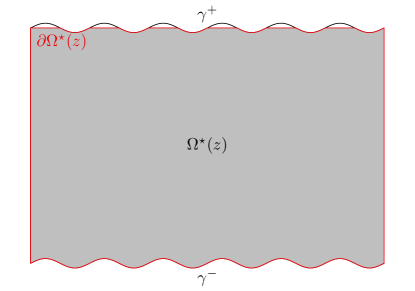
Figure 3: Illustration of $\Omega^{\star}(z)$

Integrate the previous equation in $z$ between $\min h$ and $1+\max h$ and write

$$\int_{\min h}^{1+\max h}\int_{\partial\Omega^{\star}(z)}n\cdot(\nabla T-uT)\,dS\,dz=A+B+C,$$

where

$$A =\int_{\min h}^{1+\max h}\int_{\gamma^{-}\cap\{y_{2}\leq z\}}n_{-}\cdot(\nabla T-uT)\,dS\,dz$$

$$B =\int_{\min h}^{1+\max h}\int_{\gamma^{+}\cap\{y_{2}\leq z\}}n_{+}\cdot(\nabla T-uT)\,dS\,dz$$

$$C =\int_{\min h}^{1+\max h}\int_{\Omega\cap\{y_{2}=z\}}n_{+}\cdot(\nabla T-uT)\,dS\,dz.$$

We analyze the three terms separately:

Term C: We notice that this term can be simply rewritten as

$$C=\int_{\min h}^{1+\max h}\int_{\Omega\cap\{y_{2}=z\}}(\partial_{2}T-u_{2}T)\,dS\,dz=\int_{\Omega}(\partial_{2}T-u_{2}T).$$

Term B: This integral has a sign, in fact

$$B=\int_{\min h}^{1+\max h}\int_{\gamma^{+}\cap\{y_{2}\leq z\}}n_{+}\cdot\nabla T\,dS\,dz\leq 0,$$

since, at $\gamma^{+}$ we have $n_{+}\cdot\nabla T\leq 0$.

Term A: We decompose the integral in A further:

$$A=\left(\int_{\min h}^{\max h}+\int_{\max h}^{1+\max h}\right)\int_{\gamma^{-}\cap\{y_{2}\leq z\}}n_{-}\cdot(\nabla T-uT)\,dS\,dz=:A_{1}+A_{2}.$$

Notice that

$$A_{2} =\int_{\max h}^{1+\max h}\int_{\gamma^{-}}n_{-}\cdot(\nabla T-uT)\,dS\,dz=\int_{0}^{1}dz\int_{\gamma^{-}}n_{-}\cdot(\nabla T-uT)\,dS$$

$$=\int_{\gamma^{-}}n_{-}\cdot\nabla T.$$

The term $A_{1}$ instead will be estimated as follows

$$\int_{\min h}^{\max h} \int_{\gamma^{-}\cap\{y_{2}\leq z\}}n_{-}\cdot(\nabla T-uT)\,dS\,dz$$

$$=\int_{\min h}^{\max h}\int_{\gamma^{-}\cap\{y_{2}\leq z\}}n_{-}\cdot\nabla T\,dS\,dz\leq\int_{\min h}^{\max h}\int_{\gamma^{-}}n_{-}\cdot\nabla T\,dS\,dz$$

$$=(\max h-\min h)\int_{\gamma^{-}}n_{-}\cdot\nabla T,$$

where in the first inequality we used that $n_{-}\cdot\nabla T\geq 0$ at $\gamma^{-}$.

Putting all together, we obtain

$$\int_{\min h}^{1+\max h} \int_{\partial\Omega^{\star}}n\cdot(\nabla T-uT)\,dS\,dz$$

$$\leq(1+\max h-\min h)\int_{\gamma^{-}}n_{-}\cdot\nabla T+\int_{\Omega}(\partial_{2}T-u_{2}T).$$

Taking the long-time average and observing that

$$\limsup_{t\rightarrow\infty}\frac{1}{t}\int_{0}^{t} \int_{\min h}^{1+\max h}\int_{\partial\Omega^{\star}(z)}n\cdot(\nabla T-uT)\ dS\ dz\ dt$$

$$=\limsup_{t\rightarrow\infty}\frac{1}{t}\int_{0}^{t}\int_{\min h}^{1+\max h}\int_{\Omega^{\star}(z)}(\Delta T-u\cdot\nabla T)\ dy\ dz\ dt$$

$$=\limsup_{t\rightarrow\infty}\frac{1}{t}\int_{0}^{t}\frac{d}{dt}\int_{\min h}^{1+\max h}\int_{\Omega^{\star}(z)}T\ dy\ dz\ dt=0\,$$

by the maximum principle for $T$, we have

$$0\leq(1+\max h-\min h)\langle n_{-}\cdot\nabla T\,\rangle_{\gamma^{-}}+\langle\partial_{2}T-u_{2}T\rangle$$

implying

$$\langle u_{2}T-\partial_{2}T\rangle\leq(1+\max h-\min h)\langle n_{-}\cdot\nabla T\rangle_{\gamma^{-}}.$$

∎

3 A-priori bounds

In this section we collect a-priori bounds on the energy and enstrophy of the solution $u$ and derive pressure estimates that will be used to prove the main result in the Section 4.

3.1 A-priori estimate for the velocity

Proposition 3.1 (Energy Balance).

Strong solutions of (NS), (DF), (3) satisfy

$$\frac{1}{2\rm{Pr}}\frac{d}{dt}\|u\|_{2}^{2}+\|\nabla u\|_{2}^{2}+\int_{\gamma^{+}\cup\gamma^{-}}(2\alpha+\kappa)u_{\tau}^{2}={\rm{Ra}}\int_{\Omega}Tu_{2}.$$ (17)

Proof.

The balance follows by testing the Navier Stokes equations with $u$, integrating by parts and observing that

$$\int_{\Omega}u\cdot\nabla p=0$$

and

$$\int_{\Omega}u\cdot(u\cdot\nabla)u=-\int_{\Omega}u\cdot(u\cdot\nabla)u$$

by the incompressibility and boundary conditions, and

$$\int_{\Omega}u\cdot\Delta u =-\|\nabla u\|_{2}^{2}+\int_{\partial\Omega}n_{i}u_{j}\partial_{i}u_{j}$$

$$=-\|\nabla u\|_{2}^{2}+2\int_{\gamma^{+}\cup\gamma^{-}}u\cdot(\mathbb{D}u\ n)-\int_{\gamma^{+}\cup\gamma^{-}}n_{i}u_{j}\partial_{j}u_{i}$$

$$=-\|\nabla u\|_{2}^{2}-2\int_{\gamma^{+}\cup\gamma^{-}}\alpha u_{\tau}^{2}-\int_{\gamma^{+}\cup\gamma^{-}}n\cdot(u\cdot\nabla)u$$

$$=-\|\nabla u\|_{2}^{2}-\int_{\gamma^{+}\cup\gamma^{-}}(2\alpha+\kappa)u_{\tau}^{2}\,.$$

In this identity we used the algebraic identity

$$n_{i}u_{j}\partial_{i}u_{j}=2u\cdot(\mathbb{D}u\,n)-n_{i}u_{j}\partial_{j}u_{i},$$

the Navier slip boundary conditions to deduce

$$u\cdot(\mathbb{D}u\,n)+\alpha u_{\tau}^{2}=0$$

and the equality

$$n\cdot(u\cdot\nabla)u=\kappa u_{\tau}^{2}\,,$$ (18)

proved in (84) in the Appendix.

∎

Under a smallness assumption on $\kappa$, the second and third term on the left-hand side of (17) are positive and bounded from below by the $H^{1}$-norm of $u$ even though $(2\alpha+\kappa)$ might be negative on some parts of the boundary. This will be essential in what follows, especially in order to prove the energy decay and the main theorem.

Lemma 3.2.

Assume $\alpha\geq\underline{\alpha}$ almost everywhere on $\gamma^{-}\cup\gamma^{+}$ for some constant $\underline{\alpha}>0$ and $\kappa$ satisfies

$$|\kappa|\leq 2\alpha+\frac{1}{4\sqrt{1+(h^{\prime})^{2}}}\min\left\{1,\sqrt{\alpha}\right\}$$ (19)

almost everywhere on $\gamma^{-}\cup\gamma^{+}$. Then

$$\frac{3}{4}\|\nabla u\|_{2}^{2}+\int_{\gamma^{-}\cup\gamma^{+}}(2\alpha+\kappa)u_{\tau}^{2}\geq\frac{1}{4}\min\{1,\underline{\alpha}\}\|u\|_{H^{1}}^{2}.$$ (20)

Proof.

In this proof we use the notation

$$\kappa_{-} =\kappa(y_{1},h(y_{1})), \alpha_{-} =\alpha(y_{1},h(y_{1})), u_{-} =u_{\tau}(y_{1},h(y_{1})),$$ (21)

$$\kappa_{+} =\kappa(y_{1},1+h(y_{1})), \alpha_{+} =\alpha(y_{1},1+h(y_{1})), u_{+} =u_{\tau}(y_{1},1+h(y_{1})),$$

which is the evaluation of the functions on the bottom or top boundary. Notice that, because of the symmetry of the domain, $\kappa_{-}=-\kappa_{+}$.

The idea of the proof is that if $\kappa_{-}$ is negative for some $y_{1}$, then $\kappa_{+}$ is positive and we can compensate by the fundamental theorem of calculus.

By the fundamental theorem of calculus, Young’s and Hölder’s inequality

$$|u(y_{1},y_{2})|^{2} \leq\left(u_{-}+\int_{h(y_{1})}^{y_{2}}\partial_{2}u(y_{1},z)\ dz\right)^{2}$$ (22)

$$\leq(1+\epsilon)u_{-}^{2}+(1+\epsilon^{-1})\left(\int_{h(y_{1})}^{y_{2}}\partial_{2}u(y_{1},z)\ dz\right)^{2}$$

$$\leq(1+\epsilon)u_{-}^{2}+(1+\epsilon^{-1})(y_{2}-h(y_{1}))\|\partial_{2}u\|_{L^{2}(\gamma^{-},\gamma^{+})}^{2}$$

for all $\epsilon>0$, where $\|\partial_{2}u\|_{L^{2}(\gamma^{-},\gamma^{+})}^{2}=\int_{h(y_{1})}^{1+h(y_{1})}|\partial_{2}u(y_{1},y_{2})|^{2}dy_{2}$ and analogously

$$|u(y_{1},y_{2})|^{2} \leq(1+\epsilon)u_{+}^{2}+(1+\epsilon^{-1})(1+h(y_{1})-y_{2})\|\partial_{2}u\|_{L^{2}(\gamma^{-},\gamma^{+})}^{2}.$$ (23)

Integrating (22) and (23) in $y_{2}$ one gets

$$\|u\|_{L^{2}(\gamma^{-},\gamma^{+})}^{2} \leq(1+\epsilon)\min\{u_{-}^{2},u_{+}^{2}\}+\frac{1+\epsilon^{-1}}{2}\|\partial_{2}u\|_{L^{2}(\gamma^{-},\gamma^{+})}^{2}$$ (24)

$$\leq(1+\epsilon)\max\{\alpha_{-}^{-1},\alpha_{+}^{-1},1\}\Big{(}\min\{\alpha_{-},\alpha_{+}\}\sqrt{1+(h^{\prime})^{2}}\min\{u_{-}^{2},u_{+}^{2}\}$$

$$\qquad\qquad\qquad+(2\epsilon)^{-1}\|\partial_{2}u\|_{L^{2}(\gamma^{-},\gamma^{+})}^{2}\Big{)},$$

where in the last inequality we have smuggled in the factor $\sqrt{1+(h^{\prime})^{2}}>1$. Next we claim that

$$\min\{\alpha_{-},\alpha_{+}\}\sqrt{1+(h^{\prime})^{2}}u_{i}^{2} \leq\frac{5}{16}\|\partial_{2}u\|_{L^{2}(\gamma^{-},\gamma^{+})}^{2}+(2\alpha_{-}+\kappa_{-})\sqrt{1+(h^{\prime})^{2}}u_{-}^{2}$$ (25)

$$\qquad+(2\alpha_{+}+\kappa_{+})\sqrt{1+(h^{\prime})^{2}}u_{+}^{2}$$

holds for either $i=+$ or $i=-$. Using (25), (24) turns into

$$\|u\|_{L^{2}(\gamma^{-},\gamma^{+})}^{2} \leq(1+\epsilon)\max\{\alpha_{-}^{-1},\alpha_{+}^{-1},1\}\bigg{[}(2\alpha_{-}+\kappa_{-})\sqrt{1+(h^{\prime})^{2}}u_{-}^{2}$$

$$\qquad+(2\alpha_{+}+\kappa_{+})\sqrt{1+(h^{\prime})^{2}}u_{+}^{2}+\left(\frac{5}{16}+(2\epsilon)^{-1}\right)\|\partial_{2}u\|_{L^{2}(\gamma^{-},\gamma^{+})}^{2}\bigg{]}.$$

Integrating in $y_{1}$ and choosing $\epsilon=3$ yields

$$\|u\|_{2}^{2} \leq 4\max\{\underline{\alpha}^{-1},1\}\left[\int_{\gamma^{-}\cup\gamma^{+}}(2\alpha+\kappa)u_{\tau}^{2}+\frac{1}{2}\|\partial_{2}u\|_{2}^{2}\right]$$

which implies the following bound for the $H^{1}$-norm

$$\|u\|_{H^{1}}^{2} \leq 4\max\{\underline{\alpha}^{-1},1\}\left[\int_{\gamma^{-}\cup\gamma^{+}}(2\alpha+\kappa)u_{\tau}^{2}+\frac{3}{4}\|\nabla u\|_{2}^{2}\right].$$

It is only left to show that (25) holds. In order to prove the claim we distinguish between two cases.

• If $|\kappa|\leq 2\alpha$, then both $2\alpha_{\pm}+\kappa_{\pm}>0$ and as $\kappa_{-}=-\kappa_{+}$ either $\kappa_{-}$ or $\kappa_{+}$ is non-negative. Assume first $\kappa_{-}\geq 0$. Then by these observations

  $$\min\{ \alpha_{-},\alpha_{+}\}\sqrt{1+(h^{\prime})^{2}}u_{i}^{2}$$

  $$\leq 2\alpha_{-}\sqrt{1+(h^{\prime})^{2}}u_{-}^{2}$$

  $$\leq(2\alpha_{-}+\kappa_{-})\sqrt{1+(h^{\prime})^{2}}u_{-}^{2}+(2\alpha_{+}+\kappa_{+})\sqrt{1+(h^{\prime})^{2}}u_{+}^{2}$$

  The case $\kappa_{+}>0$ follows similar with $u_{+}^{2}$ instead of $u_{-}^{2}$.

• Now assume that $\kappa_{+}<0$ and $|\kappa_{+}|>2\alpha_{+}$. The case $\kappa_{-}<0$ and $|\kappa_{-}|>2\alpha_{-}$ follows similarly by exchanging $+$ and $-$. Using (22) with $y_{2}=1+h(y_{1})$, respectively (23) with $y_{2}=h(y_{1})$, and observing that $\kappa_{-}=-\kappa_{+}>2\alpha_{+}>0$ it holds

  $$-(2\alpha_{-}+\kappa_{-}) \sqrt{1+(h^{\prime})^{2}}u_{-}^{2}-(2\alpha_{+}+\kappa_{+})\sqrt{1+(h^{\prime})^{2}}u_{+}^{2}$$

  $$=-(2\alpha_{-}+\kappa_{-})\sqrt{1+(h^{\prime})^{2}}u_{-}^{2}+(\kappa_{-}-2\alpha_{+})\sqrt{1+(h^{\prime})^{2}}u_{+}^{2}$$

  $$\leq(\kappa_{-}-2\alpha_{+})(1+\epsilon^{-1})\sqrt{1+(h^{\prime})^{2}}\|\partial_{2}u\|_{L^{2}(\gamma^{-},\gamma^{+})}^{2}$$

  $$\qquad-\left[2\alpha_{-}+2\alpha_{+}-\epsilon(\kappa_{-}-2\alpha_{+})\right]\sqrt{1+(h^{\prime})^{2}}u_{-}^{2}.$$

  In order for the squared bracket to be positive we choose $\epsilon=\frac{\alpha_{-}+\alpha_{+}}{\kappa_{-}-2\alpha_{+}}$ to get

  $$-(2\alpha_{-}+\kappa_{-}) \sqrt{1+(h^{\prime})^{2}}u_{-}^{2}-(2\alpha_{+}+\kappa_{+})\sqrt{1+(h^{\prime})^{2}}u_{+}^{2}$$

  $$\leq\left(\kappa_{-}-2\alpha_{+}+\frac{(\kappa_{-}-2\alpha_{+})^{2}}{\alpha_{-}+\alpha_{+}}\right)\sqrt{1+(h^{\prime})^{2}}\|\partial_{2}u\|_{L^{2}(\gamma^{-},\gamma^{+})}^{2}$$

  $$\qquad-\left[\alpha_{-}+\alpha_{+}\right]\sqrt{1+(h^{\prime})^{2}}u_{-}^{2}.$$

  Then, as the smallness condition (19) implies

  $$\kappa_{-} =|\kappa_{+}|\leq 2\alpha_{+}+\frac{1}{4\sqrt{1+(h^{\prime})^{2}}}\min\left\{1,\sqrt{\alpha_{+}}\right\}$$

  $$\leq 2\alpha_{+}+\frac{1}{4}\min\left\{\frac{1}{\sqrt{1+(h^{\prime})^{2}}},\frac{\sqrt{\alpha_{+}+\alpha_{-}}}{(1+(h^{\prime})^{2})^{\frac{1}{4}}}\right\},$$

  we get

  $$-(2\alpha_{-}+\kappa_{-}) \sqrt{1+(h^{\prime})^{2}}u_{-}^{2}-(2\alpha_{+}+\kappa_{+})\sqrt{1+(h^{\prime})^{2}}u_{+}^{2}$$

  $$\leq\frac{5}{16}\|\partial_{2}u\|_{L^{2}(\gamma^{-},\gamma^{+})}^{2}-\left[\alpha_{-}+\alpha_{+}\right]\sqrt{1+(h^{\prime})^{2}}u_{-}^{2},$$

  proving the claim.

∎

Remark 3.1.

Note that this Lemma can be improved: In fact for every $\kappa$ and $\alpha$ with $\kappa_{\mp}<\sqrt{\frac{2\alpha_{\mp}+2\alpha_{\pm}}{\sqrt{1+(h^{\prime})^{2}}}+(2\alpha_{\pm})^{2}}$, where we use the notation (21), it holds $\|\nabla u\|_{2}^{2}+\int(2\alpha+\kappa)u_{\tau}^{2}>0$. This implies energy decay in (17).
Nevertheless, in order to simplify the estimates and improve readability we will work with assumption (19) instead. This choice will have no effects in terms of optimality of the bounds for the Nusselt number.

We will use the energy balance and (20) to prove the following decay estimate for the energy of $u$:

Lemma 3.3 (Energy Decay).

Let the assumptions of Lemma 3.2 be satisfied. Then the energy of $u$ is bounded by

$$\|u\|_{2}^{2}\leq e^{-\frac{1}{4}\min\{1,\underline{\alpha}\}\rm{Pr}\phantom{.}t}\|u_{0}\|_{2}^{2}+256\max\left\{1,\underline{\alpha}^{-2}\right\}|\Omega|{\rm{Ra}}^{2}.$$ (26)

Proof.

By the energy balance (17), Young’s inequality and the maximum principle (11), we obtain

$$\frac{1}{2\rm{Pr}}\frac{d}{dt}\|u\|_{2}^{2} \leq-\|\nabla u\|_{2}^{2}-\int_{\gamma^{+}\cup\gamma^{-}}(2\alpha+\kappa)u_{\tau}^{2}+\epsilon\|u_{2}\|_{2}^{2}+\frac{4}{\epsilon}|\Omega|{\rm{Ra}}^{2}\,.$$ (27)

Plugging (20) into (27), we find

$$\frac{1}{2\rm{Pr}}\frac{d}{dt}\|u\|_{2}^{2} \leq-\left(\frac{1}{4}\min\{1,\underline{\alpha}\}-\epsilon\right)\|u\|_{2}^{2}+\frac{4}{\epsilon}|\Omega|{\rm{Ra}}^{2}\,,$$

and choosing $\epsilon=\frac{1}{8}\min\{1,\underline{\alpha}\}$ yields

$$\frac{d}{dt}\|u\|_{2}^{2} \leq-\frac{1}{4}\min\{1,\underline{\alpha}\}\rm{Pr}\|u\|_{2}^{2}+64\rm{Pr}\max\{1,\underline{\alpha}^{-1}\}|\Omega|{\rm{Ra}}^{2}\,.$$

Applying Grönwall’s inequality we obtain (26). ∎

Taking the long-time average of the energy balance (17), using the fact that

$$\limsup_{t\to\infty}\frac{1}{t}\int_{0}^{t}\frac{d}{dt}\|u\|_{2}^{2}=\limsup_{t\to\infty}\frac{1}{t}\left(\|u\|_{2}^{2}-\|u_{0}\|_{2}^{2}\right)=0$$

thanks to the uniform bound (26) one gets

$$\langle|\nabla u|^{2}\rangle+\langle(2\alpha+\kappa)u_{\tau}^{2}\rangle_{\gamma^{-}\cup\gamma^{+}}={\rm{Ra}}\langle Tu_{2}\rangle$$

and observing that, by (15),

$${\rm{Ra}}\langle Tu_{2}\rangle={\rm{Ra}}(\langle u_{2}T-\partial_{2}T\rangle-1)\leq{\rm{Ra}}\left((1+\max h-\min h){\rm{Nu}}-1\right),$$

we deduce the following

Corollary 3.4.

$$\langle|\nabla u|^{2}\rangle+\langle(2\alpha+\kappa)u_{\tau}^{2}\rangle_{\gamma^{+}\cup\gamma^{-}}\leq{\rm{Ra}}\left((1+\max h-\min h){\rm{Nu}}-1\right).$$ (28)

3.2 A-priori estimate for the vorticity

We now introduce the two-dimensional vorticity $\omega=\nabla^{\perp}\cdot u$, where $\nabla^{\perp}=(-\partial_{2},\partial_{1})$. It is easy to see that $\omega$ satisfies the equation

$$\frac{1}{\rm{Pr}}\left(\omega_{t}+(u\cdot\nabla)\omega\right)-\Delta\omega ={\rm{Ra}}\partial_{1}T \Omega,$$ in (29)

$$\omega =-2(\alpha+\kappa)u_{\tau} \gamma^{\pm}.$$ on

Notice that the boundary term is deduced from the following computation

$$\omega =\omega(\tau\cdot\tau)=\omega(-\tau_{1}n_{2}+\tau_{2}n_{1})=\tau_{i}n_{j}(-\partial_{i}u_{j}+\partial_{j}u_{i})$$

$$=2\tau\cdot\mathbb{D}u\cdot n-2n\cdot(\tau\cdot\nabla)u=-2(\alpha+\kappa)u_{\tau},$$

where we used that $\tau=(-n_{2},n_{1})$, the boundary conditions (3) and the identity

$$\kappa u_{\tau}=n\cdot(\tau\cdot\nabla)u,$$ (30)

proved in (83) in the Appendix.

Proposition 3.5.

The following vorticity balance holds

$$\frac{1}{2\rm{Pr}}\frac{d}{dt} \|\omega\|^{2}+\frac{1}{\rm{Pr}}\frac{d}{dt}\int_{\gamma^{-},\gamma^{+}}(\alpha+\kappa)u_{\tau}^{2}+\|\nabla\omega\|_{2}^{2}-{\rm{Ra}}\int_{\Omega}\omega\partial_{1}T$$

$$=-2\int_{\gamma^{-}\cup\gamma^{+}}(\alpha+\kappa)u\cdot\nabla p-\frac{2}{3\rm{Pr}}\int_{\gamma^{-}\cup\gamma^{+}}(\alpha+\kappa)u\cdot(u\cdot\nabla)u$$

$$\qquad-2{\rm{Ra}}\int_{\gamma^{-}}(\alpha+\kappa)u_{\tau}n_{1}.$$

Proof.

Testing the vorticity equation with $\omega$ yields

$$\frac{1}{2\rm{Pr}}\frac{d}{dt}\|\omega\|_{2}^{2}=-\frac{1}{\rm{Pr}}\int_{\Omega}\omega(u\cdot\nabla)\omega+\int_{\Omega}\omega\Delta\omega+{\rm{Ra}}\int_{\Omega}\omega\partial_{1}T$$ (31)

Using the incompressibility condition, it is easy to see that the first term on the right-hand side vanishes since $u\cdot n=0$ at $\partial\Omega$. In order to analyze the second term, we first notice that

$$n\cdot\nabla\omega=\tau\cdot\Delta u=\frac{1}{\rm{Pr}}\tau\cdot u_{t}+\frac{1}{\rm{Pr}}\tau\cdot(u\cdot\nabla)u+\tau\cdot\nabla p-{\rm{Ra}}Tn_{1}\,,$$ (32)

where we used incompressibility in the first identity. Then, using the boundary conditions for the vorticity and temperature and (32), we have

$$\int_{\Omega}\omega\Delta\omega =-\|\nabla\omega\|_{2}^{2}+\int_{\gamma^{-}\cup\gamma^{+}}\omega n\cdot\nabla\omega$$

$$=-\|\nabla\omega\|_{2}^{2}-2\int_{\gamma^{-}\cup\gamma^{+}}(\alpha+\kappa)u_{\tau}n\cdot\nabla\omega$$

$$=-\|\nabla\omega\|_{2}^{2}-\frac{2}{\rm{Pr}}\int_{\gamma^{-}\cup\gamma^{+}}(\alpha+\kappa)u_{\tau}\tau\cdot u_{t}-\frac{2}{\rm{Pr}}\int_{\gamma^{-}\cup\gamma^{+}}(\alpha+\kappa)u_{\tau}\tau\cdot(u\cdot\nabla)u$$

$$\qquad-2\int_{\gamma^{-}\cup\gamma^{+}}(\alpha+\kappa)u_{\tau}\tau\cdot\nabla p+2{\rm{Ra}}\int_{\gamma^{-}\cup\gamma^{+}}(\alpha+\kappa)u_{\tau}Tn_{1}$$

$$=-\|\nabla\omega\|_{2}^{2}-\frac{1}{\rm{Pr}}\frac{d}{dt}\int_{\gamma^{-}\cup\gamma^{+}}(\alpha+\kappa)u_{\tau}^{2}-\frac{2}{\rm{Pr}}\int_{\gamma^{-}\cup\gamma^{+}}(\alpha+\kappa)u\cdot(u\cdot\nabla)u$$

$$\qquad-2\int_{\gamma^{-}\cup\gamma^{+}}(\alpha+\kappa)u\cdot\nabla p+2{\rm{Ra}}\int_{\gamma^{-}}(\alpha+\kappa)u_{\tau}n_{1}\,.$$

Plugging it into (31) yields

$$\frac{1}{2\rm{Pr}}\frac{d}{dt}\|\omega\|_{2}^{2} =\int_{\Omega}\omega\Delta\omega+{\rm{Ra}}\int_{\Omega}\omega\partial_{1}T$$

$$=-\|\nabla\omega\|_{2}^{2}-\frac{1}{\rm{Pr}}\frac{d}{dt}\int_{\gamma^{-}\cup\gamma^{+}}(\alpha+\kappa)u_{\tau}^{2}-\frac{2}{\rm{Pr}}\int_{\gamma^{-}\cup\gamma^{+}}(\alpha+\kappa)u\cdot(u\cdot\nabla)u$$

$$\qquad-2\int_{\gamma^{-}\cup\gamma^{+}}(\alpha+\kappa)u\cdot\nabla p-2{\rm{Ra}}\int_{\gamma^{-}}(\alpha+\kappa)u_{\tau}n_{1}+{\rm{Ra}}\int_{\Omega}\omega\partial_{1}T\,.$$

Let us observe that the term $\int(\alpha+\kappa)u\cdot(u\cdot\nabla)u$ is, in general, non-zero as the parameters $\alpha$ and $\kappa$ depend on the space variables. ∎

We now want to relate the $L^{2}$-norm of the vorticity with the $L^{2}$-norm of the enstrophy.

Lemma 3.6.

Let $2\leq q\leq p$. If $h\in W^{3,\infty}$ and $\omega\in W^{1,p}$

$$\|\nabla u\|_{2}^{2} =\|\omega\|_{2}^{2}+\int_{\gamma^{-}\cup\gamma^{+}}\kappa u_{\tau}^{2}$$

$$\|u\|_{W^{1,p}} \leq C\left(\|\omega\|_{p}+\left(1+\|\kappa\|_{\infty}^{1+\frac{2}{q}-\frac{2}{p}}\right)\|u\|_{q}\right)$$

$$\|u\|_{W^{2,p}} \leq C\left(\|\nabla\omega\|_{p}+(1+\|\kappa\|_{\infty})\|\omega\|_{p}+\left(1+\|\kappa\|_{\infty}^{2}+\|\dot{\kappa}\|_{\infty}\right)\|u\|_{p}\right)$$

holds, where the constant $C$ only depends on $p$, $|\Omega|$ and $\|h^{\prime}\|_{\infty}$.

Remark 3.2.

Note that in the case of flat boundaries the estimates simplify to

$$\|\nabla u\|_{2}^{2}=\|\omega\|_{2}^{2},\qquad\|\nabla u\|_{W^{m,p}}\leq C\|\omega\|_{W^{m,p}}$$

as proven in Lemma 7 in [DNN22].

Proof.

• Integrating by parts twice, we find

  $$\|\nabla u\|_{2}^{2} =\int_{\gamma^{-}\cup\gamma^{+}}u\cdot(n\cdot\nabla)u-\int u\cdot\Delta u$$ (33)

  $$=\int_{\gamma^{-}\cup\gamma^{+}}u\cdot(n\cdot\nabla)u+\int u^{\perp}\cdot\nabla\omega$$

  $$=\int_{\gamma^{-}\cup\gamma^{+}}u\cdot(n\cdot\nabla)u-\int_{\gamma^{-}\cup\gamma^{+}}u_{\tau}\omega+\|\omega\|_{2}^{2},$$

  where we used the identity

  $$\nabla^{\perp}\omega=\begin{pmatrix}\partial_{2}^{2}u_{1}-\partial_{1}\partial_{2}u_{2}\\ -\partial_{1}\partial_{2}u_{1}+\partial_{1}^{2}u_{2}\end{pmatrix}=\Delta u,$$

  due to incompressibility. Next notice that $\tau_{i}\tau_{j}+n_{i}n_{j}=\delta_{ij}$. Therefore the second boundary term of the right-hand side of (33) can be rewritten as

  $$-\int_{\gamma^{-}\cup\gamma^{+}}u_{\tau}\omega =-\int_{\gamma^{-}\cup\gamma^{+}}u_{\tau}\tau\cdot(\tau\cdot\nabla^{\perp})u-\int_{\gamma^{-}\cup\gamma^{+}}u_{\tau}n\cdot(n\cdot\nabla^{\perp})u$$ (34)

  $$=-\int_{\gamma^{-}\cup\gamma^{+}}u\cdot(n\cdot\nabla)u+\int_{\gamma^{-}\cup\gamma^{+}}n\cdot(u\cdot\nabla)u,$$

  where in the last identity we used that $\tau\cdot\nabla^{\perp}=-\tau^{\perp}\cdot\nabla=n\cdot\nabla$ and $u_{\tau}n\cdot\nabla^{\perp}=-u_{\tau}\cdot n^{\perp}\cdot\nabla=-u_{\tau}\tau\cdot\nabla=-u\cdot\nabla$. The first term on the right-hand side of (33) cancels with the first term on the right-hand side of (34), implying

  $$\|\nabla u\|_{2}^{2}=\int_{\gamma^{-}\cup\gamma^{+}}n\cdot(u\cdot\nabla)u+\|\omega\|_{2}^{2}$$

  Finally using

  $$n\cdot(u\cdot\nabla)u=\kappa u_{\tau}^{2}$$ (35)

  on $\gamma^{-}\cup\gamma^{+}$, which is proven in (84) in the Appendix, yields the claim.

• Let $\phi$ be the stream function of $u$, i.e. $\nabla^{\perp}\phi=u$, then

  $$\Delta\phi =\omega$$

  $$\phi|_{\gamma^{\pm}} =\phi_{\pm}$$

  with constants $\phi_{+}$ and $\phi_{-}$ and without loss of generality set $\phi_{-}=0$. We can calculate $\phi_{+}$ by

  $$\phi_{+} =\frac{1}{|\Omega|}\int_{0}^{\Gamma}\phi_{+}dy_{1}=\frac{1}{|\Omega|}\int_{0}^{\Gamma}\left[\phi_{-}+\int_{h(y_{1})}^{1+h(y_{1})}\partial_{2}\phi\ dy_{2}\right]dy_{1}=-\frac{1}{|\Omega|}\int_{\Omega}u_{1}\ dy.$$

  Therefore $\bar{\phi}=\phi+(y_{2}-h(y_{1}))\frac{1}{|\Omega|}\int_{\Omega}u_{1}\ dy$ solves

  $$\Delta\bar{\phi} =\omega-h^{\prime\prime}\frac{1}{|\Omega|}\int_{\Omega}u_{1}\ dy$$

  $$\bar{\phi}|_{\gamma^{\pm}} =0.$$

  In order to flatten the boundary we introduce the change of variables

  $$x=\Phi(y)=\begin{pmatrix}y_{1}\\ y_{2}-h(y_{1})\end{pmatrix},\qquad y=\Psi(x)=\begin{pmatrix}x_{1}\\ x_{1}+h(x_{1})\end{pmatrix}.$$

  Here and in the rest of the paper $C>0$ denotes a constant that possibly depends on $\|h^{\prime}\|_{\infty}$, the size of the domain $|\Omega|$ and the Sobolev exponent and may change from line to line. Note that

  $$\|h^{\prime}\|_{\infty}\leq C,\qquad\|h^{\prime\prime}\|_{\infty}\leq C\|\kappa\|_{\infty},\qquad\|h^{\prime\prime\prime}\|_{\infty}\leq C(\|\dot{\kappa}\|_{\infty}+\|\kappa\|_{\infty}),$$

  and for $\xi(x)=\chi(\Psi(x))=\chi(y)$ one has

  $$\|\nabla\xi\|_{p} \leq C\|\nabla\chi\|_{p}$$ (36)

  $$\|\nabla^{2}\xi\|_{p} \leq C(\|\nabla^{2}\chi\|_{p}+\|\kappa\|_{\infty}\|\nabla\chi\|_{p})$$

  $$\|\nabla^{3}\xi\|_{p} \leq C\left(\|\nabla^{3}\chi\|_{p}+\|\kappa\|_{\infty}\|\nabla^{2}\chi\|_{p}+(\|\dot{\kappa}\|_{\infty}+\|\kappa\|_{\infty})\|\nabla\chi\|_{p}\right)$$

  and analogous for the transformation in the other direction. Then

  $$\tilde{L}\tilde{\phi} =\tilde{f} [0,\Gamma]\times[0,1]$$ in (37)

  $$\tilde{\phi} =0 [0,\Gamma]\times\{x_{2}=0\}\cup\{x_{2}=1\},$$ on

  where $\tilde{L}\tilde{\phi}=\sum_{i,j}\partial_{x_{i}}(\tilde{a}_{i,j}\partial_{x_{j}}\tilde{\phi}(x))$ with $\tilde{a}_{1,1}=1$, $\tilde{a}_{1,2}=\tilde{a}_{2,1}=-h^{\prime}$ and $\tilde{a}_{2,2}=1+(h^{\prime})^{2}$, $\tilde{\phi}(x)=\bar{\phi}(\Psi(x))$ and $\tilde{f}=\tilde{\omega}-h^{\prime\prime}\frac{1}{|\Omega|}\int_{\Omega}u_{1}dy$ with $\tilde{\omega}(x)=\omega(\Psi(x))$. As this operator is elliptic we get

  $$\|\tilde{\phi}\|_{W^{2,p}}\leq C\|\tilde{f}\|_{p}$$ (38)

  for some constant $C>0$ depending only on $p$, $|\Omega|$ and $\|h^{\prime}\|_{\infty}$. Using Hölder’s inequality and the estimates for the change of variables (36), (38) becomes

  $$\|\tilde{\phi}\|_{W^{2,p}}\leq C\|\tilde{f}\|_{p}\leq C\|\omega\|_{p}+C\|\kappa\|_{\infty}\|u\|_{p}.$$ (39)

  Going back to the definition of $\bar{\phi}$, we find that (36), Hölder’s inequality and (39) yield

  $$\|\nabla u\|_{p} =\|\nabla^{2}\phi\|_{p}\leq\|\nabla^{2}\bar{\phi}\|_{p}+C\|h^{\prime\prime}\|_{\infty}\|u_{1}\|_{1}$$ (40)

  $$\leq C\left(\|\nabla^{2}\tilde{\phi}\|_{p}+\|\kappa\|_{\infty}\|\nabla\tilde{\phi}\|_{p}+\|h^{\prime\prime}\|_{\infty}\|u_{1}\|_{1}\right)$$

  $$\leq C\left(\|\omega\|_{p}+\|\kappa\|_{\infty}\|u\|_{p}\right),$$

  implying

  $$\|u\|_{W^{1,p}} \leq C\left(\|\omega\|_{p}+(1+\|\kappa\|_{\infty})\|u\|_{p}\right).$$ (41)

  In order to estimate the $L^{p}$-norm of $u$ by the $L^{q}$-norm use interpolation and Young’s inequality to get

  $$\|u\|_{p}\leq C\|\nabla u\|_{p}^{\theta}\|u\|_{q}^{1-\theta}+C\|u\|_{q}\leq\epsilon\theta C\|\nabla u\|_{p}+C\left((1-\theta)\epsilon^{-\frac{\theta}{1-\theta}}+1\right)\|u\|_{q}$$

  for $\frac{1}{p}=\theta\left(\frac{1}{p}-\frac{1}{2}\right)+\frac{1-\theta}{q}$ and all $\epsilon>0$. Then choosing $\epsilon^{-1}=(1+\|\kappa\|_{\infty})$ and plugging in $\theta=\frac{2(q-p)}{2(q-p)-pq}$

  $$(1+\|\kappa\|_{\infty})\|u\|_{p} \leq C\|\nabla u\|_{p}+C\left(1+\|\kappa\|_{\infty}^{\frac{1}{1-\theta}}\right)\|u\|_{q}$$

  $$\leq C\|\nabla u\|_{p}+C\left(1+\|\kappa\|_{\infty}^{1+\frac{2}{q}-\frac{2}{p}}\right)\|u\|_{q}$$

  proving the claim.

• In order to prove the $W^{2,p}$ bound notice that by (37) $\hat{\phi}=\partial_{x_{1}}\tilde{\phi}$ solves

  $$\tilde{L}\hat{\phi} =\hat{f} [0,\Gamma]\times[0,1]$$ in

  $$\hat{\phi} =0 \{x_{2}=0\}\cup\{x_{2}=1\},$$ on

  with $\hat{f}=\partial_{x_{1}}\tilde{\omega}+h^{\prime\prime\prime}\frac{1}{|\Omega|}\int_{\Omega}u_{1}dy+\partial_{x_{1}}(h^{\prime\prime}\partial_{x_{2}}\tilde{\phi})+\partial_{x_{2}}(h^{\prime\prime}\partial_{x_{1}}\tilde{\phi})-2h^{\prime}h^{\prime\prime}\partial_{x_{2}}^{2}\tilde{\phi}\in L^{p}$. Again using elliptic regularity and Hölder’s inequality we find

  $$\|\partial_{x_{1}}\tilde{\phi}\|_{W^{2,p}} =\|\hat{\phi}\|_{W^{2,p}}\leq C\|\hat{f}\|_{p}$$ (42)

  $$\leq C\left(\|\nabla\tilde{\omega}\|_{p}+\|\dot{\kappa}\|_{\infty}(\|u\|_{p}+\|\nabla\tilde{\phi}\|_{p})+\|\kappa\|_{\infty}\|\nabla^{2}\tilde{\phi}\|_{p}\right).$$

  In order to estimate the missing term $\partial_{x_{2}}^{3}\tilde{\phi}$ notice as $h^{\prime}$ is independent of $x_{2}$

  $$\partial_{x_{2}}^{3}\tilde{\phi} =\frac{1}{1+(h^{\prime})^{2}}\partial_{x_{2}}\left(\partial_{x_{2}}((1+(h^{\prime})^{2})\partial_{x_{2}}\tilde{\phi}\right)$$ (43)

  $$=\frac{1}{1+(h^{\prime})^{2}}\partial_{x_{2}}\left(\tilde{L}\tilde{\phi}-\partial_{x_{1}}^{2}\tilde{\phi}+\partial_{x_{1}}(h^{\prime}\partial_{x_{2}}\tilde{\phi})+\partial_{x_{2}}(h^{\prime}\partial_{x_{1}}\tilde{\phi})\right)$$

  $$=\frac{1}{1+(h^{\prime})^{2}}\partial_{x_{2}}\left(\tilde{f}-\partial_{x_{1}}^{2}\tilde{\phi}+\partial_{x_{1}}(h^{\prime}\partial_{x_{2}}\tilde{\phi})+\partial_{x_{2}}(h^{\prime}\partial_{x_{1}}\tilde{\phi})\right).$$

  Taking the norm in (43) we find

  $$\|\partial_{x_{2}}^{3}\tilde{\phi}\|_{p} \leq C\left(\|\nabla\tilde{f}\|_{p}+\|\kappa\|_{\infty}\|\partial_{x_{2}}^{2}\tilde{\phi}\|_{p}+\|\partial_{x_{1}}\tilde{\phi}\|_{W^{2,p}}\right).$$ (44)

  Combining (42) and (44)

  $$\|\tilde{\phi}\|_{W^{3,p}}\leq C\left(\|\nabla\tilde{f}\|_{p}+\|\kappa\|_{\infty}\|\nabla^{2}\tilde{\phi}\|_{p}+\|\nabla\tilde{\omega}\|_{p}+\|\dot{\kappa}\|_{\infty}(\|u\|_{p}+\|\nabla\tilde{\phi}\|_{p})\right).$$

  Using Hölder’s inequality we find

  $$\|\nabla\tilde{f}\|_{p}\leq C(\|\nabla\tilde{\omega}\|_{p}+\|\dot{\kappa}\|_{\infty}\|u\|_{p}),$$

  which together with (39) yields

  $$\|\tilde{\phi}\|_{W^{3,p}} \leq C\left(\|\nabla\tilde{\omega}\|_{p}+\|\kappa\|_{\infty}\|\omega\|_{p}+\|\kappa\|_{\infty}^{2}\|u\|_{p}+\|\dot{\kappa}\|_{\infty}(\|u\|_{p}+\|\nabla\tilde{\phi}\|_{p})\right)$$ (45)

  $$\leq C\left(\|\nabla\omega\|_{p}+\|\kappa\|_{\infty}\|\omega\|_{p}+(\|\kappa\|_{\infty}^{2}+\|\dot{\kappa}\|_{\infty})\|u\|_{p}\right),$$

  where in the last inequality we used

  $$\|\nabla\tilde{\omega}\|_{p}\leq C\|\nabla\omega\|_{p},\qquad\|\nabla\tilde{\phi}\|_{p}\leq C\|\nabla\bar{\phi}\|_{p}\leq C(\|\nabla\phi\|_{p}+\|u_{1}\|_{1})\leq C\|u\|_{p}.$$ (46)

  By the definitions and the change of variables estimate (36) and Hölder’s inequality one gets

  $$\|\nabla^{2}u\|_{p} =\|\nabla^{3}\phi\|_{p}\leq\|\nabla^{3}\bar{\phi}\|_{p}+h^{\prime\prime\prime}\frac{1}{|\Omega|}\int|u_{1}|$$

  $$\leq C\left(\|\nabla^{3}\tilde{\phi}\|_{p}+\|\kappa\|_{\infty}\|\nabla^{2}\tilde{\phi}\|_{p}+(\|\dot{\kappa}\|_{\infty}+\|\kappa\|_{\infty})\|\nabla\tilde{\phi}\|_{p}+\|\kappa\|_{\infty}\|u\|_{p}\right)$$

  $$\leq C\left(\|\nabla\omega\|_{p}+\|\kappa\|_{\infty}\|\omega\|_{p}+(\|\kappa\|_{\infty}+\|\kappa\|_{\infty}^{2}+\|\dot{\kappa}\|_{\infty})\|u\|_{p}\right),$$

  where in the last inequality we used (45), (39) and (46). Finally using the $W^{1,r}$-bound for $u$, (41), and Young’s inequality yields the claim.

∎

The next result concerns a crucial $L_{t}^{\infty}L^{p}_{x}-$bound for the vorticity.

Lemma 3.7.

Let $p\in(2,\infty)$ and assume that the conditions of Lemma 3.2 are satisfied. Then there exists a constant $C$ depending only on $p$, $|\Omega|$ and $\|h^{\prime}\|_{\infty}$ such that

$$\|\omega\|_{p} \leq C\left[\|\omega_{0}\|_{p}+\left(1+\|\alpha+\kappa\|_{\infty}^{\frac{2(p-1)}{p-2}}\right)\|u_{0}\|_{2}+C_{\alpha,\kappa}{\rm{Ra}}\right],$$

where $C_{\alpha,\kappa}=\left(1+\|\alpha+\kappa\|_{\infty}^{\frac{2(p-1)}{p-2}}\right)\max\left\{1,\underline{\alpha}^{-1}\right\}$.

Proof.

Fix an arbitrary time $\bar{t}>0$ and decompose the solution $\omega$ to (29) as

$$\omega=\bar{\omega}_{\pm}+\tilde{\omega}_{\pm}$$

where $\tilde{\omega}_{\pm}$ solves

$$\frac{1}{\rm{Pr}}(\partial_{t}\tilde{\omega}_{\pm}+u\cdot\nabla\tilde{\omega}_{\pm})-\Delta\tilde{\omega}_{\pm} ={\rm{Ra}}\partial_{1}T \Omega$$ in

$$\tilde{\omega}_{\pm} =\pm\Lambda \gamma^{+}\cup\gamma^{-}$$ on

$$\tilde{\omega}_{\pm,0} =\pm|\omega_{0}| \Omega\,,$$ in

with $\Lambda=2\|(\alpha+\kappa)u_{\tau}\|_{L^{\infty}([0,\bar{t}]\times\{\gamma^{+}\cup\gamma^{-}\})}$ and the difference $\bar{\omega}_{\pm}=\omega-\tilde{\omega}_{\pm}$ solves

$$\frac{1}{\rm{Pr}}(\partial_{t}\bar{\omega}_{\pm}+u\cdot\nabla\bar{\omega}_{\pm})-\Delta\bar{\omega}_{\pm} =0 \Omega$$ in

$$\bar{\omega}_{\pm} =-2(\alpha+\kappa)u_{\tau}\mp\Lambda \gamma^{+}\cup\gamma^{-}$$ on

$$\bar{\omega}_{\pm,0} =\omega_{0}\mp|\omega_{0}| \Omega\,.$$ in

Since the boundary and the initial values have a sign, i.e. $\bar{\omega}_{+}\leq 0$ on $\gamma^{+}\cup\gamma^{-}$, $\bar{\omega}_{+,0}\leq 0$ in $\Omega$ and $\bar{\omega}_{-}\geq 0$ on $\gamma^{+}\cup\gamma^{-}$, $\bar{\omega}_{-,0}\geq 0$ in $\Omega$, then, by the maximum principle, $\omega-\tilde{\omega}_{+}=\bar{\omega}_{+}\leq 0$ and $0\leq\bar{\omega}_{-}=\omega-\tilde{\omega}_{-}$ yielding $\tilde{\omega}_{-}\leq\omega\leq\tilde{\omega}_{+}$. In particular

$$|\omega|\leq\max\{|\tilde{\omega}_{-}|,|\tilde{\omega}_{+}|\}\,.$$ (47)

Hence, it remains to find upper bounds for $|\tilde{\omega}_{-}|$ and $|\tilde{\omega}_{+}|$. By symmetry, it suffices to show an upper bound for $\tilde{\omega}_{+}$. We divide the proof in three steps:

Step 1: Omitting the indices, we define

$$\hat{\omega}=\tilde{\omega}-\Lambda,$$

then $\hat{\omega}$ satisfies

$$\frac{1}{\rm{Pr}}(\partial_{t}\hat{\omega}+u\cdot\nabla\hat{\omega})-\Delta\hat{\omega} ={\rm{Ra}}\partial_{1}T \Omega$$ in

$$\hat{\omega} =\Lambda-\Lambda=0 \gamma^{+}\cup\gamma^{-}$$ on

$$\hat{\omega}_{0} =|\omega_{0}|-\Lambda \Omega\,.$$ in

Testing the equation with $\hat{\omega}|\hat{\omega}|^{p-2}$ we obtain

$$\frac{1}{p\rm{Pr}}\frac{d}{dt}\|\hat{\omega}\|_{p}^{p} =-(p-1)\int_{\Omega}|\nabla\hat{\omega}|^{2}|\hat{\omega}|^{p-2}-{\rm{Ra}}\int_{\Omega}T\partial_{1}(|\hat{\omega}|^{p-2}\hat{\omega}).$$

Using $\|T\|_{\infty}=1$, Young’s and Hölder’s inequality, we estimate the second term of the right-hand side as

$$\left|{\rm{Ra}}\int_{\Omega}T\partial_{1}(|\hat{\omega}|^{p-2}\hat{\omega})\right|\leq\frac{p-1}{2}\left({\rm{Ra}}^{2}|\Omega|^{\frac{2}{p}}\|\hat{\omega}\|_{p}^{p-2}+\int_{\Omega}|\nabla\hat{\omega}|^{2}|\hat{\omega}|^{p-2}\right).$$

Then

$$\frac{1}{p\rm{Pr}}\frac{d}{dt}\|\hat{\omega}\|_{p}^{p} \leq\frac{p-1}{2}\left({\rm{Ra}}^{2}|\Omega|^{\frac{2}{p}}\|\hat{\omega}\|_{p}^{p-2}-\int_{\Omega}|\nabla\hat{\omega}|^{2}|\hat{\omega}|^{p-2}\right)$$

$$=\frac{p-1}{2}\left({\rm{Ra}}^{2}|\Omega|^{\frac{2}{p}}\|\hat{\omega}\|_{p}^{p-2}-\frac{4}{p^{2}}\big{\|}\nabla|\hat{\omega}|^{\frac{p}{2}}\big{\|}_{2}^{2}\right).$$

By the Poincaré estimate applied to the second term of the right-hand side (remember that $\hat{\omega}$ vanishes at the boundary by definition), we obtain

$$\frac{1}{p\rm{Pr}}\frac{d}{dt}\|\hat{\omega}\|_{p}^{p}\leq\frac{p-1}{2}{\rm{Ra}}^{2}|\Omega|^{\frac{2}{p}}\|\hat{\omega}\|_{p}^{p-2}-2\frac{p-1}{p^{2}C_{p}^{2}}\|\hat{\omega}\|_{p}^{p}\,,$$

where $C_{p}$ denotes the Poincaré constant. Dividing through by $\|\hat{\omega}\|_{p}^{p-2}$ we obtain the inequality

$$\frac{d}{dt}\|\hat{\omega}\|_{p}^{2}\leq\frac{p-1}{p}\rm{Pr}{\rm{Ra}}^{2}|\Omega|^{\frac{2}{p}}-4\rm{Pr}\frac{p-1}{p^{3}C_{p}^{2}}\|\hat{\omega}\|_{p}^{2}.$$

By the Grönwall inequality

$$\|\hat{\omega}\|_{p}^{2} \leq e^{-4\rm{Pr}\frac{p-1}{p^{3}C_{p}^{2}}t}\|\hat{\omega}_{0}\|_{p}^{2}+\frac{1}{4}C_{p}^{2}p^{2}{\rm{Ra}}^{2}|\Omega|^{\frac{2}{p}}\leq e^{-4\rm{Pr}\frac{p-1}{p^{3}C_{p}^{2}}t}\|\omega_{0}-\Lambda\|_{p}^{2}+\frac{1}{4}C_{p}^{2}p^{2}{\rm{Ra}}^{2}|\Omega|^{\frac{2}{p}}$$

$$\leq e^{-4\rm{Pr}\frac{p-1}{p^{3}C_{p}^{2}}t}(\|\omega_{0}\|_{p}^{2}+\Lambda^{2}|\Omega|^{\frac{2}{p}})+\frac{1}{4}C_{p}^{2}p^{2}{\rm{Ra}}^{2}|\Omega|^{\frac{2}{p}}\leq C^{2}(\|\omega_{0}\|_{p}^{2}+\Lambda^{2}+{\rm{Ra}}^{2}).$$

Step 2: We now turn to the estimate for $\Lambda$. We have

$$\Lambda=2\|(\alpha+\kappa)u_{\tau}\|_{L^{\infty}(\gamma^{-}\cup\gamma^{+})}\leq 2\|\alpha+\kappa\|_{\infty}\|u\|_{L^{\infty}(\Omega\times[0,\bar{t}])},$$

which can be bounded using interpolation and Young’s inequality by

$$2 \|\alpha+\kappa\|_{\infty}\|u\|_{L^{\infty}(\Omega\times[0,\bar{t}])}$$

$$\qquad\leq C\|\alpha+\kappa\|_{\infty}\|\nabla u\|_{L^{\infty}_{t}(L^{p}_{x})}^{\theta}\|u\|_{L^{\infty}_{t}(L^{2}_{x})}^{1-\theta}+C\|\alpha+\kappa\|_{\infty}\|u\|_{L^{\infty}_{t}(L^{2}_{x})}$$

$$\qquad\leq\epsilon C\theta\|\nabla u\|_{L^{\infty}_{t}(L^{p}_{x})}+C\left[1+(1-\theta)\epsilon^{\frac{p}{2-p}}\|\alpha+\kappa\|_{\infty}^{\frac{p}{p-2}}\right]\|\alpha+\kappa\|_{\infty}\|u\|_{L^{\infty}_{t}(L^{2}_{x})}$$

for $p>2$ and arbitrary $\epsilon>0$, where $\theta=\frac{p}{2(p-1)}$ and $L_{t}^{\infty}(L_{x}^{p})=L^{\infty}([0,\bar{t}];L^{p}(\Omega))$. According to Lemma 3.6

$$\|u\|_{W^{1,p}} \leq C\left(\|\omega\|_{p}+\left(1+\|\kappa\|_{\infty}^{2-\frac{2}{p}}\right)\|u\|_{2}\right)$$

resulting in

$$\Lambda \leq\epsilon C\|\omega\|_{L_{t}^{\infty}(L_{x}^{p})}+C\left[\epsilon\left(1+\|\kappa\|_{\infty}^{2-\frac{2}{p}}\right)+\|\alpha+\kappa\|_{\infty}+\epsilon^{\frac{p}{2-p}}\|\alpha+\kappa\|_{\infty}^{\frac{2(p-1)}{p-2}}\right]\|u\|_{L^{\infty}_{t}(L^{2}_{x})}.$$

Step 3: Recalling that $|\omega|\leq\max\{|\tilde{\omega}_{-}|,|\tilde{\omega}_{+}|\}$ and $\hat{\omega}_{+}=\tilde{\omega}_{+}-\Lambda$ and using the results of Step 1 and Step 2 one gets

$$\|\omega\|_{L_{t}^{\infty}(L_{x}^{p})} \leq\|\tilde{\omega}\|_{L_{t}^{\infty}(L_{x}^{p})}=\|\hat{\omega}+\Lambda\|_{L_{t}^{\infty}(L_{x}^{p})}\leq\|\hat{\omega}\|_{L_{t}^{\infty}(L_{x}^{p})}+|\Omega|^{\frac{1}{p}}\Lambda\leq C(\|\omega_{0}\|_{p}+{\rm{Ra}}+\Lambda)$$

$$\leq\epsilon C\|\omega\|_{L_{t}^{\infty}(L_{x}^{p})}+C\|\omega_{0}\|_{p}+C{\rm{Ra}}$$

$$\qquad+C\left[\epsilon\left(1+\|\kappa\|_{\infty}^{2-\frac{2}{p}}\right)+\|\alpha+\kappa\|_{\infty}+\epsilon^{\frac{p}{2-p}}\|\alpha+\kappa\|_{\infty}^{\frac{2(p-1)}{p-2}}\right]\|u\|_{L^{\infty}_{t}(L^{2}_{x})}$$

Choosing $\epsilon$ small we can compensate the vorticity term on the right-hand side. By symmetry of the two boundaries $\max_{\gamma^{-}\cup\gamma^{+}}\kappa=-\min_{\gamma^{-}\cup\gamma^{+}}\kappa$, which, as $\alpha>0$, implies $\|\kappa\|_{\infty}\leq\|\alpha+\kappa\|_{\infty}$. Combining these observations we find

$$\|\omega\|_{L_{t}^{\infty}(L_{x}^{p})}\leq C\|\omega_{0}\|_{p}+C\left(1+\|\alpha+\kappa\|_{\infty}^{\frac{2(p-1)}{p-2}}\right)\|u\|_{L_{t}^{\infty}(L_{x}^{2})}+C{\rm{Ra}}.$$

Finally Lemma 3.3 yields

$$\|\omega\|_{L_{t}^{\infty}(L_{x}^{p})} \leq C\left[\|\omega_{0}\|_{p}+\left(1+\|\alpha+\kappa\|_{\infty}^{\frac{2(p-1)}{p-2}}\right)\|u_{0}\|_{2}+C_{\alpha,\kappa}{\rm{Ra}}\right],$$

where $C_{\alpha,\kappa}=\left(1+\|\alpha+\kappa\|_{\infty}^{\frac{2(p-1)}{p-2}}\right)\max\left\{1,\underline{\alpha}^{-1}\right\}$ and $C$ only depends on $|\Omega|$, $\|h^{\prime}\|_{\infty}$ and $p$. As the constants are independent of $\bar{t}$ this bound holds universally in time.

∎

As $\Omega$ is bounded Hölder inequality and Lemma 3.7 yield that if $\omega_{0}\in L^{p}$ for any $p<\infty$ then $\|\omega\|_{p}$ is universally bounded in time. By trace Theorem and Lemma 3.6

$$\|u\|_{L^{2}(\gamma^{-}\cup\gamma^{+})}\leq\|u\|_{H^{1}}\leq C\left(\|\omega\|_{2}+(1+\|\kappa\|_{\infty})\|u\|_{2}\right).$$

Using Lemma 3.3 this is also universally bounded in time, therefore taking the long time average of the vorticity balance, see Lemma 3.5, we get the following.

Corollary 3.8.

Assume that the conditions of Lemma 3.7 are satisfied and $\omega_{0}\in L^{p}$ for some $p>2$, then

$$0 =\langle|\nabla\omega|^{2}\rangle-2\langle(\alpha+\kappa)u\cdot\nabla p\rangle_{\gamma^{-}\cup\gamma^{+}}-{\rm{Ra}}\langle\omega\partial_{1}T\rangle$$ (48)

$$\qquad+\frac{2}{3\rm{Pr}}\langle(\alpha+\kappa)u\cdot(u\cdot\nabla)u\rangle_{\gamma^{-}\cup\gamma^{+}}+2{\rm{Ra}}\langle(\alpha+\kappa)u_{\tau}n_{1}\rangle_{\gamma^{-}}.$$

3.3 A-priori estimate for the pressure

The pressure satisfies

$$\Delta p =-\frac{1}{\rm{Pr}}(\nabla u)^{T}\colon\nabla u+{\rm{Ra}}\partial_{2}T \Omega$$ in (49)

$$n\cdot\nabla p =-\frac{1}{\rm{Pr}}\kappa u^{2}+2\tau\cdot\nabla\left((\alpha+\kappa)u_{\tau}\right) \gamma^{+}$$ on

$$n\cdot\nabla p =-\frac{1}{\rm{Pr}}\kappa u^{2}+2\tau\cdot\nabla\left((\alpha+\kappa)u_{\tau}\right)+n_{2}{\rm{Ra}} \gamma^{-}$$ on

The equation in the bulk is easy to obtain by applying the divergence to the Navier-Stokes equations, using incompressibility and writing compactly $\nabla\cdot((u\cdot\nabla)u)=(\nabla u)^{T}:\nabla u$. In order to track the pressure at the boundary we look at Navier-Stokes equations at $\gamma^{-}\cup\gamma^{+}$

$$\left(\frac{1}{\rm{Pr}}\left(u_{t}+(u\cdot\nabla)u\right)-\Delta u+\nabla p-{\rm{Ra}}Te_{2}\right)\cdot n=0$$

where $n$ is the normal at the boundary. It is clear that

$$n\cdot u_{t} =\frac{d}{dt}(n\cdot u)=0$$

and

$$n\cdot\Delta u=n\cdot\nabla^{\perp}\omega=-2n\cdot\nabla^{\perp}\left((\alpha+\kappa)u_{\tau}\right)=2\tau\cdot\nabla\left((\alpha+\kappa)u_{\tau}\right),$$

using the boundary condition for the vorticity in (29). Thanks to (84) in the Appendix we also have

$$n\cdot(u\cdot\nabla)u=\kappa u_{\tau}^{2}.$$ (50)

Hence

$$n\cdot\nabla p=-\frac{\kappa}{\rm{Pr}}u_{\tau}^{2}+2\tau\cdot\nabla((\alpha+\kappa)u_{\tau})+n_{2}T{\rm{Ra}}$$

at the boundary. Now, it is only left to observe that $T=0$ at $\gamma^{+}$ and $T=1$ at $\gamma^{-}$.

Proposition 3.9.

For any $r\in(2,\infty)$ there exists a constant $C$ depending on $|\Omega|$, $r$ and $\|h^{\prime}\|_{\infty}$ such that

$$\|p\|_{H^{1}}\leq C\left[{\rm{Ra}}\|T\|_{2}+\|\alpha+\kappa\|_{\infty}\|u\|_{H^{2}}+\left(\frac{1+\|\kappa\|_{\infty}}{\rm{Pr}}\|u\|_{W^{1,r}}+\|\dot{\alpha}+\dot{\kappa}\|_{\infty}\right)\|u\|_{H^{1}}\right].$$

Proof.

On one hand, integrating by parts and using the boundary conditions (for $u$ and $T$), we have

$$\int_{\Omega}p\Delta p =-\|\nabla p\|_{2}^{2}-\frac{1}{\rm{Pr}}\int_{\gamma^{-}\cup\gamma^{+}}p\kappa u_{\tau}^{2}+2\int_{\gamma^{-}\cup\gamma^{+}}p\tau\cdot\nabla\left((\alpha+\kappa)u_{\tau}\right)+{\rm{Ra}}\int_{\gamma^{-}}pn_{2}$$

On the other hand using the equation satisfied by the pressure (49)

$$\int_{\Omega}p\Delta p =-\frac{1}{\rm{Pr}}\int_{\Omega}p(\nabla u)^{T}\colon\nabla u+{\rm{Ra}}\int_{\Omega}p\partial_{2}T$$

$$=-\frac{1}{\rm{Pr}}\int_{\Omega}p(\nabla u)^{T}\colon\nabla u+{\rm{Ra}}\int_{\gamma^{-}\cup\gamma^{+}}pTn_{2}-{\rm{Ra}}\int_{\Omega}T\partial_{2}p$$

$$=-\frac{1}{\rm{Pr}}\int_{\Omega}p(\nabla u)^{T}\colon\nabla u+{\rm{Ra}}\int_{\gamma^{-}}pn_{2}-{\rm{Ra}}\int_{\Omega}T\partial_{2}p,$$

where we used the boundary conditions for $T$ in the last identity. Combining these estimates one gets

$$\|\nabla p\|^{2} =-\frac{1}{\rm{Pr}}\int_{\gamma^{-}\cup\gamma^{+}}p\kappa u_{\tau}^{2}+2\int_{\gamma^{-}\cup\gamma^{+}}p\tau\cdot\nabla\left((\alpha+\kappa)u_{\tau}\right)+\frac{1}{\rm{Pr}}\int_{\Omega}p(\nabla u)^{T}\colon\nabla u$$

$$\qquad+{\rm{Ra}}\int_{\Omega}T\partial_{2}p.$$

We estimate the right-hand side: By Hölder inequality with $\frac{1}{r}+\frac{1}{q}+\frac{1}{2}=1$ and Sobolev embedding

$$\|p(\nabla u)^{T}\colon\nabla u\|_{1} \leq\|p\|_{q}\|\nabla u\|_{2}\|\nabla u\|_{r}\leq C\|p\|_{H^{1}}\|\nabla u\|_{2}\|\nabla u\|_{r},$$ (51)

where $C$ depends on $|\Omega|$, $r$ and $\|h^{\prime}\|_{\infty}$. For the temperature term we apply Hölder’s inequality use that $\|T\|_{\infty}\leq 1$ by the maximum principle (11)

$$\|T\partial_{2}p\|_{1}\leq\|T\|_{2}\|p\|_{H^{1}}\leq|\Omega|^{\frac{1}{2}}\|p\|_{H^{1}}\,,$$

and for the second term we compute

$$\int_{\gamma^{-}\cup\gamma^{+}}\left|p\tau\cdot\nabla((\alpha+\kappa)u_{\tau})\right|$$

$$\quad\leq\|\alpha+\kappa\|_{\infty}\|p\|_{L^{2}(\gamma^{-}\cup\gamma^{+})}\|\nabla u\|_{L^{2}(\gamma^{-}\cup\gamma^{+})}+\|\dot{\alpha}+\dot{\kappa}\|_{\infty}\|p\|_{L^{2}(\gamma^{-}\cup\gamma^{+})}\|u\|_{L^{2}(\gamma^{-}\cup\gamma^{+})}$$

$$\quad\leq C\|\alpha+\kappa\|_{\infty}\|p\|_{H^{1}}\|u\|_{H^{2}}+C\|\dot{\alpha}+\dot{\kappa}\|_{\infty}\|p\|_{H^{1}}\|u\|_{H^{1}},$$

where in the last inequality we use the trace estimate. Finally, we estimate the first term: Similar to (51) for $\frac{1}{r}+\frac{1}{q}+\frac{1}{2}=1$ and every $r>2$

$$\left|\int_{\gamma^{-}\cup\gamma^{+}}\kappa pu_{\tau}^{2}\right| \leq\|\kappa\|_{\infty}\|pu_{\tau}^{2}\|_{L^{1}(\gamma^{-}\cup\gamma^{+})}$$

$$\leq C\|\kappa\|_{\infty}\|pu^{2}\|_{W^{1,1}}$$

$$\leq C\|\kappa\|_{\infty}\left(\|p\|_{q}\|u\|_{2}\|u\|_{r}+\|\nabla p\|_{2}\|u\|_{r}\|u\|_{q}+\|p\|_{q}\|u\|_{r}\|\nabla u\|_{2}\right)$$

$$\leq C\|\kappa\|_{\infty}\left(\|p\|_{H^{1}}\|u\|_{H^{1}}\|u\|_{W^{1,r}}+\|\nabla p\|_{2}\|u\|_{r}\|u\|_{H^{1}}+\|p\|_{H^{1}}\|u\|_{r}\|\nabla u\|_{2}\right)$$

$$\leq C\|\kappa\|_{\infty}\|p\|_{H^{1}}\|u\|_{H^{1}}\|u\|_{W^{1,r}}\,,$$

where $C$ depends on $|\Omega|$, $r$ and $\|h^{\prime}\|_{\infty}$.

Combining the estimates we find

$$\|\nabla p\|_{2}^{2} \leq C\|p\|_{H^{1}}\left[{\rm{Ra}}+\|\alpha+\kappa\|_{\infty}\|u\|_{H^{2}}+\left(\frac{1+\|\kappa\|_{\infty}}{\rm{Pr}}\|u\|_{W^{1,r}}+\|\dot{\alpha}+\dot{\kappa}\|_{\infty}\right)\|u\|_{H^{1}}\right].$$

Using that the pressure $p$ is only defined up to a constant so we choose $p$ to have zero mean such that Poincaré yields $\|p\|_{q}\leq C\|\nabla p\|_{q}$ which implies $\|p\|_{H^{1}}^{2}=\|\nabla p\|_{2}^{2}+\|p\|_{2}^{2}\leq(1+C^{2})\|\nabla p\|_{2}^{2}$. Then

$$\|p\|_{H^{1}}^{2} \leq C\|p\|_{H^{1}}\left[{\rm{Ra}}+\|\alpha+\kappa\|_{\infty}\|u\|_{H^{2}}+\left(\frac{1+\|\kappa\|_{\infty}}{\rm{Pr}}\|u\|_{W^{1,r}}+\|\dot{\alpha}+\dot{\kappa}\|_{\infty}\right)\|u\|_{H^{1}}\right]\,.$$

Finally dividing by $\|p\|_{H^{1}}$ we conclude that there exists a constant $C>0$ depending on $\Omega$ and $r$ such that

$$\|p\|_{H^{1}}\leq C\left[{\rm{Ra}}+\|\alpha+\kappa\|_{\infty}\|u\|_{H^{2}}+\left(\frac{1+\|\kappa\|_{\infty}}{\rm{Pr}}\|u\|_{W^{1,r}}+\|\dot{\alpha}+\dot{\kappa}\|_{\infty}\right)\|u\|_{H^{1}}\right]\,.$$

for any $r>2$. ∎

4 Upper bounds on the Nusselt number

Combining the a-priori estimates derived in the previous section we are now able to prove the ${\rm{Ra}}^{\frac{1}{2}}$ bound, that was first derived for the flat, no slip case in 3 dimensions by Doering and Constantin [DC96].

4.1 Proof of Theorem 1.1

Let $\Omega_{\delta}$ be given by

$$\Omega_{\delta}=\{(y_{1},y_{2})\ |\ 0\leq y_{1}\leq\Gamma,1+h(y_{1})-\delta\leq y_{2}\leq 1+h(y_{1})\}$$

as illustrated in Figure 4.

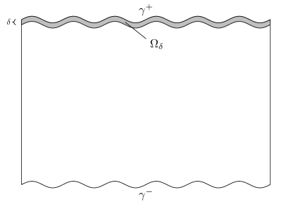
Figure 4: Illustration of $\Omega_{\delta}$.

Taking the average in $z\in(1-\delta,1)$ in the representation of the Nusselt number (14) we find

$${\rm{Nu}} =\limsup_{T\to\infty}\frac{1}{T}\int_{0}^{T}\frac{1}{\delta}\frac{1}{|\Omega|}\int_{1-\delta}^{1}\int_{\gamma(z)}n_{+}\cdot(u-\nabla)T\ dS\ dz\ dt$$ (52)

$$=\limsup_{T\to\infty}\frac{1}{T}\int_{0}^{T}\frac{1}{\delta}\frac{1}{|\Omega|}\int_{\Omega_{\delta}}n_{+}\cdot uT\ dy\ dt-\limsup_{T\to\infty}\frac{1}{T}\int_{0}^{T}\frac{1}{\delta}\frac{1}{|\Omega|}\int_{\Omega_{\delta}}n_{+}\cdot\nabla T\ dy\ dt$$

In order to estimate the first term on the right-hand side notice that by the fundamental theorem of calculus for $(y_{1},y_{2})\in\Omega_{\delta}$

$$|n_{+}\cdot u|(y_{1},y_{2}) =\left|n_{+}\cdot u|_{\gamma^{+}}+\int_{1+h(y_{1})}^{y_{2}}\partial_{2}(n_{+}\cdot u)\ dz\right|\leq\int_{1+h(y_{1})-\delta}^{1+h(y_{1})}|\partial_{2}u|\ dz$$ (53)

$$\leq\delta^{\frac{1}{2}}\|\nabla u\|_{L^{2}(\gamma^{-},\gamma^{+})},$$

where $\|\nabla u\|_{L^{2}(\gamma^{-},\gamma^{+})}=\|\nabla u(y_{1},\cdot)\|_{L^{2}(h(y_{1}),1+h(y_{1}))}$ and we used the non-penetration boundary condition for $u$ and that $n_{+}$ is constant in $y_{2}$-direction in the first inequality and Hölder’s inequality in the second estimate. Analogously for the temperature and $(y_{1},y_{2})\in\Omega_{\delta}$ it holds

$$|T|(y_{1},y_{2})\leq\delta^{\frac{1}{2}}\|\nabla T\|_{L^{2}(\gamma^{-},\gamma^{+})}$$ (54)

as $T=0$ on $\gamma^{+}$. In order to estimate the second integral in (52) partial integration and the boundary condition $T=0$ on $\gamma^{+}$ yields

$$\left|\int_{\Omega_{\delta}}n_{+}\cdot\nabla T\ dy\right|\leq\int_{\gamma^{+}}|T|\ dS+\int_{\gamma(1-\delta)}|n_{+}\cdot n_{-}T|\ dS+\int_{\Omega_{\delta}}|T\nabla\cdot n_{+}|\ dy.$$ (55)

By the maximum principle (11) the temperature is bounded by $\|T\|_{\infty}\leq 1$, so the first two terms on the right-hand side of (55) are bounded by a constant depending on $\|h^{\prime}\|_{\infty}$ and $|\Omega|$. In order to estimate the last term notice that

$$n_{+}=\frac{1}{\sqrt{1+(h^{\prime})^{2}}}\begin{pmatrix}-h^{\prime}\\ 1\end{pmatrix}\qquad\textnormal{ and }\qquad|\kappa|=\frac{|h^{\prime\prime}|}{(1+(h^{\prime})^{2})^{\frac{3}{2}}},$$

where $h^{\prime}=\partial_{1}h(y_{1})$ and $h^{\prime\prime}=\partial_{1}^{2}h(y_{1})$ as derived in (80) and (82) in the Appendix. Therefore $|\nabla\cdot n_{+}|=|\kappa|$, which implies

$$\int_{\Omega_{\delta}}|T\nabla\cdot n_{+}|\ dy\leq\|\kappa\|{{}_{\infty}}|\Omega_{\delta}|$$

for the last term in (55). Combining these observations

$$\left|\int_{\Omega_{\delta}}n_{+}\cdot\nabla T\ dy\right|\leq C(1+\delta\|\kappa\|_{\infty}).$$ (56)

Plugging (53), (54) and (56) into (52) and using Hölder inequality, there exists a constant depending on $\|h^{\prime}\|_{\infty}$ and $|\Omega|$ such that

$${\rm{Nu}} \leq\limsup_{T\to\infty}\frac{1}{T}\int_{0}^{T}\frac{1}{|\Omega|}\int_{\Omega_{\delta}}\|\nabla u\|_{L^{2}(\gamma^{-},\gamma^{+})}\|\nabla T\|_{L^{2}(\gamma^{-},\gamma^{+})}\ dy\ dt+C\left(\frac{1}{\delta}+\|\kappa\|_{\infty}\right)$$

$$\leq C\left(\delta\langle|\nabla u|^{2}\rangle^{\frac{1}{2}}\langle|\nabla T|^{2}\rangle^{\frac{1}{2}}+\frac{1}{\delta}+\|\kappa\|_{\infty}\right).$$

By (12) and (28) we can substitute both gradients and get

$${\rm{Nu}} \leq C\left(\delta{\rm{Ra}}^{\frac{1}{2}}\left((1+\max h-\min h){\rm{Nu}}-1\right)^{\frac{1}{2}}{\rm{Nu}}^{\frac{1}{2}}+\frac{1}{\delta}+\|\kappa\|_{\infty}\right)$$

$$\leq C\left(\delta{\rm{Ra}}^{\frac{1}{2}}{\rm{Nu}}+\frac{1}{\delta}+\|\kappa\|_{\infty}\right).$$

Balancing the terms by choosing $\delta={\rm{Nu}}^{-\frac{1}{2}}{\rm{Ra}}^{-\frac{1}{4}}$ we get

$${\rm{Nu}}\leq C\left({\rm{Ra}}^{\frac{1}{2}}+\|\kappa\|_{\infty}\right)$$

for ${\rm{Ra}}\geq 1$.

4.2 Introduction of the background field method

In order to improve the bound of Theorem 1.1 we follow the ”background field” strategy used [DNN22], which is based on [WD11]. This approach consists of specifying a stationary background field for the temperature and show its ”marginal stability” as we will explain in what follows. This will be achieved by applying the a-priori bounds derived in Section 3.

To this end we define the background profile for the temperature by

$$\eta(y_{1},y_{2})=1-\frac{1}{2\delta}\begin{cases}\begin{aligned} &2\delta+y_{2}-(1+h(y_{1}))&&\textnormal{for}&1+h(y_{1})-\delta&\leq y_{2}\leq 1+h(y_{1})\\ &\delta&&\textnormal{for}&h(y_{1})+\delta&<y_{2}<1+h(y_{1})-\delta\\ &y_{2}-h(y_{1})&&\textnormal{for}&h(y_{1})&\leq y_{2}\leq h(y_{1})+\delta\end{aligned}\end{cases}$$ (57)

for $\delta>0$ and the difference $\theta$ by

$$\theta=T-\eta.$$ (58)

This profile is illustrated in Figure 5.

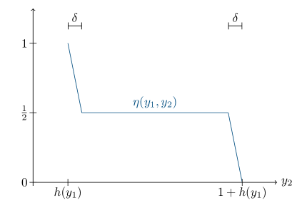
Figure 5: Illustrations of the background profile $\eta$.

Note that $\eta$ fulfills the boundary conditions of $T$, so $\theta$ vanishes on $\gamma^{\pm}$. Also since $n_{-}$ can be expressed by

$$n_{-}=\frac{1}{\sqrt{1+(h^{\prime})^{2}}}\begin{pmatrix}h^{\prime}\\ -1\end{pmatrix}$$

as derived in (80), its gradient is given by

$$\nabla\eta=\begin{cases}\begin{aligned} &0&&\textnormal{for}&h(y_{1})+\delta<y_{2}<1+h(y_{1})-\delta\\ &\frac{1}{2\delta}\sqrt{1+(h^{\prime})^{2}}n_{-}&&\textnormal{else}\end{aligned}\end{cases}$$ (59)

for almost every $y\in\Omega$. Inserting this decomposition in the definition of the Nusselt number, we have

Proposition 4.1.

Let $\eta$ and $\theta$ be defined by (57) and (58). Then

$${\rm{Nu}}=\langle|\nabla\eta|^{2}\rangle-\langle|\nabla\theta|^{2}\rangle-2\langle\theta u\cdot\nabla\eta\rangle$$ (60)

The proof of this identity is essentially the same as the one for Proposition 7 in [DNN22] and we report it here just for convenience of the reader.

Proof.

Plugging the definitions of $\eta$ and $\theta$ into (AD) we have

$$\theta_{t}+u\cdot\nabla\eta+u\cdot\nabla\theta-\Delta\eta-\Delta\theta=0,$$

and, integrating this equation against $\theta$ we find

$$0=\frac{1}{2}\frac{d}{dt}\|\theta\|_{2}^{2}+\int_{\Omega}\theta u\cdot\nabla\eta+\int_{\Omega}\theta u\cdot\nabla\theta-\int_{\Omega}\theta\Delta\eta-\int_{\Omega}\theta\Delta\theta.$$ (61)

The third term on the right-hand side of (61) vanishes since $u\cdot n=0$ and $u$ is divergence-free. For the fourth term on the right-hand side of (61) we get

$$-\int_{\Omega}\theta\Delta\eta =-\int_{\gamma^{-}\cup\gamma^{+}}\theta n\cdot\nabla\eta+\int_{\Omega}\nabla\theta\cdot\nabla\eta=\int_{\Omega}\nabla\theta\cdot\nabla\eta,$$

where in the last equality we used that $\theta$ vanishes on the boundary by definition. Similarly

$$-\int_{\Omega}\theta\Delta\theta=\|\nabla\theta\|_{2}^{2}.$$

Therefore taking the long time average of (61) and using that $\theta$ is universally bounded in time as both $T$ and $\eta$ fulfill $0\leq T,\eta\leq 1$ we find

$$\langle\theta u\cdot\nabla\eta\rangle+\langle\nabla\theta\cdot\nabla\eta\rangle+\langle|\nabla\theta|^{2}\rangle=0.$$

Using this identity in the definition of the Nusselt number (12) we find

$${\rm{Nu}}=\langle|\nabla T|^{2}\rangle=\langle|\nabla\eta|^{2}\rangle+2\langle\nabla\theta\cdot\nabla\eta\rangle+\langle|\nabla\theta|^{2}\rangle=\langle|\nabla\eta|^{2}\rangle-\langle|\nabla\theta|^{2}\rangle-2\langle\theta u\cdot\nabla\eta\rangle$$

as a representation of ${\rm{Nu}}$. ∎

Next we define

$$\mathbf{a} :=\langle|\nabla\omega|^{2}\rangle-2\langle(\alpha+\kappa)u\cdot\nabla p\rangle_{\gamma^{-}\cup\gamma^{+}}-{\rm{Ra}}\langle\omega\partial_{1}T\rangle$$

$$\qquad+\frac{2}{3\rm{Pr}}\langle(\alpha+\kappa)u\cdot(u\cdot\nabla)u\rangle_{\gamma^{-}\cup\gamma^{+}}+2{\rm{Ra}}\langle(\alpha+\kappa)u_{\tau}n_{1}\rangle_{\gamma^{-}}=0,$$

where the last identity is due to (48) and

$$\mathbf{b} :=\langle|\nabla u|^{2}\rangle+\langle(2\alpha+\kappa)u_{\tau}^{2}\rangle_{\gamma^{-}\cup\gamma^{+}}-{\rm{Ra}}\left((1+\max h-\min h){\rm{Nu}}-1\right)\,.$$ (62)

Using (60) we can rewrite the Nusselt number as

$$(1-b(1+ \max h-\min h)){\rm{Nu}}+b=M{\rm{Ra}}^{2}+2\langle|\nabla\eta|^{2}\rangle-\mathcal{Q}[u,\theta,\eta]$$ (63)

where the quadratic form $\mathcal{Q}$ is defined as

$$\mathcal{Q}[u,\theta,\eta]:=M{\rm{Ra}}^{2}+\langle|\nabla\eta|^{2}\rangle+\langle|\nabla\theta|^{2}\rangle+2\langle\theta u\cdot\nabla\eta\rangle\\ \qquad+\frac{b}{{\rm{Ra}}}\langle|\nabla u|^{2}\rangle+\frac{b}{{\rm{Ra}}}\langle(2\alpha+\kappa)u_{\tau}^{2}\rangle_{\gamma^{-}\cup\gamma^{+}}-\frac{b}{{\rm{Ra}}}\mathbf{b}+a\mathbf{a}\,.$$ (64)

In this new representation $a>0$ and $0\leq b<(1+\max h-\min h)^{-1}$ and notice that the balancing term $M{\rm{Ra}}^{2}$, with $M>0$, was introduced. The choice of the parameters $a,b,M$ will follow from an optimization procedure at the end.

We now want to prove that for a suitable choice of $\delta$ the form $\mathcal{Q}$ is non negative. In order to do so we need the following Lemma.

Lemma 4.2.

One has

$$2|\langle\theta u\cdot\nabla\eta\rangle| \leq\delta^{6}C(a\epsilon)^{-1}\langle|\partial_{2}u|^{2}\rangle+a\epsilon\langle|\partial_{2}^{2}u|^{2}\rangle+\frac{1}{2}\langle|\partial_{2}\theta|^{2}\rangle$$

for any $\epsilon>0$.

Proof.

By (59)

$$2\int_{\Omega}\theta u\cdot\nabla\eta =\frac{1}{\delta}\int_{0}^{\Gamma}\int_{h(y_{1})}^{h(y_{1})+\delta}\sqrt{1+(h^{\prime})^{2}}\theta u\cdot n_{-}\ dy_{2}\ dy_{1}$$ (65)

$$\qquad+\frac{1}{\delta}\int_{0}^{\Gamma}\int_{1+h(y_{1})-\delta}^{1+h(y_{1})}\sqrt{1+(h^{\prime})^{2}}\theta u\cdot n_{-}\ dy_{2}\ dy_{1}$$

We focus on the first term on the right-hand side. The second one can be treated similarly. By the fundamental theorem of calculus and Hölder’s inequality

$$|u\cdot n_{-}|(y_{1},y_{2}) =\left|(u\cdot n_{-})(y_{1},h(y_{1}))+\int_{h(y_{1})}^{y_{2}}\partial_{2}(u\cdot n_{-})(y_{1},z)\ dz\right|$$ (66)

$$\leq\delta\|\partial_{2}(u\cdot n_{-})\|_{L^{\infty}(\gamma^{-},\gamma^{+})}$$

for $h(y_{1})\leq y_{2}\leq h(y_{1})+\delta$, where in the last inequality we used the boundary condition for $u$. Similarly

$$|\theta(y_{1},y_{2})|\leq\delta^{\frac{1}{2}}\|\partial_{2}\theta\|_{L^{2}(\gamma^{-},\gamma^{+})}$$ (67)

as $\theta$ vanishes on the boundary. In order to estimate $\partial_{2}(n_{-}\cdot u)$ notice that by partial integration and the boundary condition for $u$

$$\int_{h(y_{1})}^{1+h(y_{1})}\partial_{2}(n_{-}\cdot u)=n_{2}\ n_{-}\cdot u|_{\gamma^{-}}-n_{2}\ n_{-}\cdot u|_{\gamma^{+}}=0.$$

Therefore for every $y_{1}$ there exists $h(y_{1})\leq\bar{y}_{2}\leq 1+h(y_{1})$ such that $\partial_{2}(u\cdot n_{-})(y_{1},\bar{y}_{2})=0$. Applying the fundamental theorem of calculus again we find

$$(\partial_{2}(u\cdot n_{-}))^{2}(y_{1},y_{2}) =(\partial_{2}(u\cdot n_{-}))^{2}(y_{1},\bar{y}_{2})+\int_{\bar{y}_{2}}^{y_{2}}\partial_{2}\left((\partial_{2}(u\cdot n_{-}))^{2}\right)(y_{1},z)\ dz$$ (68)

$$\leq 2\|\partial_{2}u\|_{L^{2}(\gamma^{-},\gamma^{+})}\|\partial_{2}^{2}u\|_{L^{2}(\gamma^{-},\gamma^{+})},$$

where in the last inequality we used Hölder’s inequality, that $n_{-}$ is constant in $e_{2}$ direction and $|n_{-}|=1$. Combing (65) with (66), (67) and (68) and using Young’s inequality twice yields

$$\bigg{|}2\int_{\Omega} \theta u\cdot\nabla\eta\ dy\bigg{|}$$

$$\leq(2\delta)^{\frac{3}{2}}\int_{0}^{\Gamma}\|\partial_{2}u\|_{L^{2}(\gamma^{-},\gamma^{+})}^{\frac{1}{2}}\|\partial_{2}^{2}u\|_{L^{2}(\gamma^{-},\gamma^{+})}^{\frac{1}{2}}\|\partial_{2}\theta\|_{L^{2}(\gamma^{-},\gamma^{+})}\sqrt{1+(h^{\prime})^{2}}\ dy_{1}$$

$$\leq C\delta^{\frac{3}{2}}\int_{0}^{\Gamma}\mu\nu\|\partial_{2}u\|_{L^{2}(\gamma^{-},\gamma^{+})}^{2}+\mu\nu^{-1}\|\partial_{2}^{2}u\|_{L^{2}(\gamma^{-},\gamma^{+})}^{2}+\mu^{-1}\|\partial_{2}\theta\|_{L^{2}(\gamma^{-},\gamma^{+})}^{2}\ dy_{1}$$

for some $\mu,\nu>0$ that will be determined later and $C=\left\|\sqrt{1+(h^{\prime})^{2}}\right\|_{\infty}$.

Taking the long time average

$$2|\langle\theta u\cdot\nabla\eta\rangle|\leq C\delta^{\frac{3}{2}}\left(\mu\nu\langle|\partial_{2}u|^{2}\rangle+\mu\nu^{-1}\langle|\partial_{2}^{2}u|^{2}\rangle+\mu^{-1}\langle|\partial_{2}\theta|^{2}\rangle\right)$$

and setting $\mu=2\delta^{\frac{3}{2}}C$ and $\nu=2\delta^{3}C^{2}(a\epsilon)^{-1}$ yields the result. ∎

With all these preparations at hand we are able to prove the main result in the next subsection.

4.3 Proof of Theorem 1.2

In the following we will extensively use

$$\underline{\alpha}\leq 1,\qquad\|\kappa\|_{\infty}\leq 1.$$ (69)

The first inequality is justified as $\operatorname*{ess\,inf}\alpha\leq\operatorname*{ess\,inf}_{\kappa>0}(\alpha+\kappa)\leq\|\alpha+\kappa\|_{\infty}\leq 1$ by assumption (6) and the second one as $\kappa(y_{1},h(y_{1}))=-\kappa(y_{1},1+h(y_{1}))$ and $\alpha>0$ almost everywhere one has $-\operatorname*{ess\,inf}_{\kappa<0}\kappa=\operatorname*{ess\,sup}_{\kappa>0}\kappa\leq\operatorname*{ess\,sup}_{\kappa>0}\alpha+\kappa\leq\|\alpha+\kappa\|_{\infty}\leq 1$ by assumption (6).

We will show that $\mathcal{Q}$ is non-negative for some appropriate choice of $\delta$. Then (63) will yield the bound.

As $\mathbf{b}\leq 0$ by (28) plugging in the definition of $\mathbf{a}$, i.e. (4.2), yields

$$\mathcal{Q}[u,\theta,\eta] =M{\rm{Ra}}^{2}+\langle|\nabla\eta|^{2}\rangle+\langle|\nabla\theta|^{2}\rangle+2\langle\theta u\cdot\nabla\eta\rangle+\frac{b}{{\rm{Ra}}}\langle|\nabla u|^{2}\rangle+\frac{b}{{\rm{Ra}}}\langle(2\alpha+\kappa)u_{\tau}^{2}\rangle_{\gamma^{-}\cup\gamma^{+}}$$ (70)

$$\qquad-\frac{b}{{\rm{Ra}}}\mathbf{b}+a\mathbf{a}$$

$$\geq M{\rm{Ra}}^{2}+\langle|\nabla\eta|^{2}\rangle+\langle|\nabla\theta|^{2}\rangle+2\langle\theta u\cdot\nabla\eta\rangle+\frac{b}{{\rm{Ra}}}\langle|\nabla u|^{2}\rangle+\frac{b}{{\rm{Ra}}}\langle(2\alpha+\kappa)u_{\tau}^{2}\rangle_{\gamma^{-}\cup\gamma^{+}}$$

$$\qquad+a\langle|\nabla\omega|^{2}\rangle-2a\langle(\alpha+\kappa)u\cdot\nabla p\rangle_{\gamma^{-}\cup\gamma^{+}}-a{\rm{Ra}}\langle\omega\partial_{1}T\rangle$$

$$\qquad+\frac{2}{3\rm{Pr}}a\langle(\alpha+\kappa)u\cdot(u\cdot\nabla)u\rangle_{\gamma^{-}\cup\gamma^{+}}+2a{\rm{Ra}}\langle(\alpha+\kappa)u_{\tau}n_{1}\rangle_{\gamma^{-}}.$$

Next we estimate some of the terms individually.

• For the eighth term on the right-hand side of (70) we can shift the derivative onto $u$ and $\alpha+\kappa$ as the boundary is periodic and get

  $$-\int_{\gamma^{-}\cup\gamma^{+}}(\alpha+\kappa)u\cdot\nabla p\ dS =\langle p\tau\cdot\nabla((\alpha+\kappa)u_{\tau})\rangle_{\gamma^{-}\cup\gamma^{+}}$$

  $$=\langle(\alpha+\kappa)p\tau\cdot\nabla u_{\tau}\rangle_{\gamma^{-}\cup\gamma^{+}}+\langle p(\dot{\alpha}+\dot{\kappa})u_{\tau}\rangle_{\gamma^{-}\cup\gamma^{+}}$$

  Using Hölder’s inequality and Trace Theorem one gets

  $$\left|\int_{\gamma^{-}\cup\gamma^{+}}(\alpha+\kappa)u\cdot\nabla p\ dS\right|\leq C\left(\|\alpha+\kappa\|_{\infty}\|u\|_{H^{2}}+\|\dot{\alpha}+\dot{\kappa}\|_{\infty}\|u\|_{H^{1}}\right)\|p\|_{H^{1}}$$

  where $\dot{\alpha}$ and $\dot{\kappa}$ denotes the derivative of $\alpha$ and $\kappa$ along the boundary. The pressure bound derived in Proposition 3.9 and Young’s inequality imply

  $$2\left|\int_{\gamma^{-}\cup\gamma^{+}}(\alpha+\kappa)u\cdot\nabla p\ dS\right|$$ (71)

  $$\qquad\leq C\left(\|\alpha+\kappa\|_{\infty}\|u\|_{H^{2}}+\|\dot{\alpha}+\dot{\kappa}\|_{\infty}\|u\|_{H^{1}}\right)$$

  $$\qquad\qquad\cdot\left[Ra\|T\|_{2}+\|\alpha+\kappa\|_{\infty}\|u\|_{H^{2}}+\left(\frac{1+\|\kappa\|_{\infty}}{\rm{Pr}}\|u\|_{W^{1,r}}+\|\dot{\alpha}+\dot{\kappa}\|_{\infty}\right)\|u\|_{H^{1}}\right]$$

  $$\qquad\leq\left(\epsilon+C\|\alpha+\kappa\|_{\infty}^{2}\right)\|u\|_{H^{2}}^{2}+C_{\epsilon}\|\alpha+\kappa\|_{W^{1,\infty}}^{2}{\rm{Ra}}^{2}$$

  $$\qquad\qquad+C\left(\left(\frac{1}{\rm{Pr}}\|u\|_{W^{1,r}}\right)^{2}+\|\alpha+\kappa\|_{W^{1,\infty}}^{2}+1\right)\|u\|_{H^{1}}^{2}$$

  for all $\epsilon>0$, where $C_{\epsilon}>0$ depends on $|\Omega|$, $r$, $\|h^{\prime}\|_{\infty}$ and $\epsilon$ and in the last inequality we used that $\|\kappa\|\leq 1$.

• For the ninth term on the right-hand side of (70) Hölder’s and Young’s inequality yield

  $$|a{\rm{Ra}}\langle\omega\partial_{1}T\rangle| =|a{\rm{Ra}}\langle\omega\partial_{1}(\eta+\theta)\rangle|\leq\frac{1}{2}\langle|\nabla\eta|^{2}\rangle+\frac{1}{2}\langle|\nabla\theta|^{2}\rangle+a^{2}{\rm{Ra}}^{2}\langle|\omega|^{2}\rangle.$$

• In order to estimate the tenth term on the right-hand side of (70) we first use Hölder’s inequality and Trace Theorem to get

  $$\frac{1}{\rm{Pr}} \left|\int_{\gamma^{-}\cup\gamma^{+}}(\alpha+\kappa)u\cdot(u\cdot\nabla)u\ dS\right|\leq C\frac{\|\alpha+\kappa\|_{\infty}}{\rm{Pr}}\left\|u^{2}|\nabla u|\right\|_{W^{1,1}}.$$ (72)

  Again Hölder’s inequality with $\frac{1}{r}+\frac{1}{p}+\frac{1}{2}=1$ and Sobolev Theorem as in the proof of Proposition 3.9 imply

  $$\left\|u^{2}|\nabla u|\right\|_{W^{1,1}} \leq C\left(\|u\|_{q}\|u\|_{r}\|\nabla u\|_{2}+\|u\|_{q}\|\nabla u\|_{r}\|\nabla u\|_{2}+\|u\|_{q}\|u\|_{r}\|\nabla^{2}u\|_{2}\right)$$ (73)

  $$\leq C\left(\|u\|_{W^{1,r}}\|u\|_{H^{1}}+\|u\|_{H^{2}}\|u\|_{W^{1,r}}\right)\|u\|_{H^{1}}$$

  for all $r>2$. Combining (72) and (73) and using Young’s inequality and the assumption $\|\alpha+\kappa\|_{\infty}\leq 1$ yields

  $$\frac{2}{3\rm{Pr}}\bigg{|}\int_{\gamma^{-}\cup\gamma^{+}}(\alpha+\kappa) u\cdot(u\cdot\nabla)u\ dS\bigg{|}$$ (74)

  $$\leq C\frac{1}{\rm{Pr}}\left(\|u\|_{W^{1,r}}\|u\|_{H^{1}}+\|u\|_{H^{2}}\|u\|_{W^{1,r}}\right)\|u\|_{H^{1}}$$

  $$\leq\epsilon\|u\|_{H^{2}}^{2}+C\left(C_{\epsilon}\left(\frac{1}{\rm{Pr}}\|u\|_{W^{1,r}}\right)^{2}+1\right)\|u\|_{H^{1}}^{2}$$

  for all $\epsilon>0$ where $C_{\epsilon}>0$ depends on $|\Omega|$, $r$, $\|h^{\prime}\|_{\infty}$ and $\epsilon$.

• In order to estimate the eleventh term on the right-hand side of (70) notice that by Trace Theorem and Young’s inequality

  $$2{\rm{Ra}}\left|\int_{\gamma^{-}\cup\gamma^{+}}(\alpha+\kappa)u_{\tau}n_{1}\ dS\right| \leq C{\rm{Ra}}\|\alpha+\kappa\|_{\infty}\|u\|_{H^{1}}\leq C\|\alpha+\kappa\|_{\infty}^{2}{\rm{Ra}}^{2}+\|u\|_{H^{1}}^{2}.$$ (75)

In order to apply these estimates we first notice that by Lemma 3.6

$$\|u\|_{W^{1,r}}\leq C\left(\|\omega\|_{r}+(1+\|\kappa\|_{\infty})^{2-\frac{2}{r}}\|u\|_{2}\right).$$

The $L^{p}$-norm of the vorticity and energy are bounded by Lemma 3.7 and Lemma 3.3 respectively, implying

$$\|u\|_{W^{1,r}}\leq C\left(\|u_{0}\|_{W^{1,r}}+\underline{\alpha}^{-1}{\rm{Ra}}\right),$$

where we exploited (69). Using this bound for the $W^{1,r}$ norm of $u$, the prefactors in the individual estimates are independent of time. Then taking the long time average of (71), (74) and (75) and plugging the bounds into (70) yields

$$\mathcal{Q}[u,\theta,\eta] \geq M{\rm{Ra}}^{2}+\frac{1}{2}\langle|\nabla\eta|^{2}\rangle+\frac{1}{2}\langle|\nabla\theta|^{2}\rangle+2\langle\theta u\cdot\nabla\eta\rangle+\frac{b}{{\rm{Ra}}}\langle|\nabla u|^{2}\rangle+\frac{b}{{\rm{Ra}}}\langle(2\alpha+\kappa)u_{\tau}^{2}\rangle_{\gamma^{-}\cup\gamma^{+}}$$

$$\qquad+a\langle|\nabla\omega|^{2}\rangle-a\left[2\epsilon+C\|\alpha+\kappa\|_{\infty}^{2}\right]\left\langle\|u\|_{H^{2}}^{2}\right\rangle-C_{\epsilon}a\|\alpha+\kappa\|_{W^{1,\infty}}^{2}{\rm{Ra}}^{2}$$

$$\qquad-aC\left[C_{\epsilon}\left(\frac{1}{\rm{Pr}}\left(\|u_{0}\|_{W^{1,r}}+\underline{\alpha}^{-1}{\rm{Ra}}\right)\right)^{2}+\|\alpha+\kappa\|_{W^{1,\infty}}^{2}+1\right]\left\langle\|u\|_{H^{1}}^{2}\right\rangle$$

$$\qquad-a^{2}{\rm{Ra}}^{2}\langle|\omega|^{2}\rangle.$$

Choosing $M=C_{\epsilon}a\|\alpha+\kappa\|_{W^{1,\infty}}^{2}$

$$\mathcal{Q}[u,\theta,\eta] \geq\frac{1}{2}\langle|\nabla\theta|^{2}\rangle+2\langle\theta u\cdot\nabla\eta\rangle+\frac{b}{{\rm{Ra}}}\langle|\nabla u|^{2}\rangle+\frac{b}{{\rm{Ra}}}\langle(2\alpha+\kappa)u_{\tau}^{2}\rangle_{\gamma^{-}\cup\gamma^{+}}$$ (76)

$$\qquad+a\langle|\nabla\omega|^{2}\rangle-a\left[2\epsilon+C\|\alpha+\kappa\|_{\infty}^{2}\right]\left\langle\|u\|_{H^{2}}^{2}\right\rangle$$

$$\qquad-aC\left[C_{\epsilon}\left(\frac{1}{\rm{Pr}}\left(\|u_{0}\|_{W^{1,r}}+\underline{\alpha}^{-1}{\rm{Ra}}\right)\right)^{2}+\|\alpha+\kappa\|_{W^{1,\infty}}^{2}+1\right]\left\langle\|u\|_{H^{1}}^{2}\right\rangle$$

$$\qquad-a^{2}{\rm{Ra}}^{2}\langle|\omega|^{2}\rangle.$$

In order to estimate the second term on the right-hand side of (76) use Lemma (4.2) to get

$$\mathcal{Q}[u,\theta,\eta] \geq\frac{b}{{\rm{Ra}}}\langle|\nabla u|^{2}\rangle+\frac{b}{{\rm{Ra}}}\langle(2\alpha+\kappa)u_{\tau}^{2}\rangle_{\gamma^{-}\cup\gamma^{+}}$$

$$\qquad+a\langle|\nabla\omega|^{2}\rangle-a\left[3\epsilon+C\|\alpha+\kappa\|_{\infty}^{2}\right]\left\langle\|u\|_{H^{2}}^{2}\right\rangle$$

$$\qquad-aC\left[C_{\epsilon}\left(\frac{1}{\rm{Pr}}\left(\|u_{0}\|_{W^{1,r}}+\underline{\alpha}^{-1}{\rm{Ra}}\right)\right)^{2}+\|\alpha+\kappa\|_{W^{1,\infty}}^{2}+1\right]\left\langle\|u\|_{H^{1}}^{2}\right\rangle$$

$$\qquad-a^{2}{\rm{Ra}}^{2}\langle|\omega|^{2}\rangle-C_{\epsilon}\delta^{6}a^{-1}\langle|\nabla u|^{2}\rangle.$$

Next according to Lemma (3.2) the first two terms on the right-hand side can be estimated by the $H^{1}$ norm, i.e.

$$\frac{3b}{8{\rm{Ra}}}\langle|\nabla u|^{2}\rangle+\frac{b}{2{\rm{Ra}}}\langle(2\alpha+\kappa)u_{\tau}^{2}\rangle_{\gamma^{-}\cup\gamma^{+}}\geq\frac{\underline{\alpha}b}{8{\rm{Ra}}}\langle\|u\|_{H^{1}}^{2}\rangle.$$ (77)

Then

$$\mathcal{Q}[u,\theta,\eta] \geq a\langle|\nabla\omega|^{2}\rangle-a\left[3\epsilon+C\|\alpha+\kappa\|_{\infty}^{2}\right]\left\langle\|u\|_{H^{2}}^{2}\right\rangle$$

$$\qquad+\left[\frac{\underline{\alpha}b}{8{\rm{Ra}}}-aC_{\epsilon}\left(\left(\frac{1}{\rm{Pr}}\left(\|u_{0}\|_{W^{1,r}}+\underline{\alpha}^{-1}{\rm{Ra}}\right)\right)^{2}+\|\alpha+\kappa\|_{W^{1,\infty}}^{2}+1\right)\right]\left\langle\|u\|_{H^{1}}^{2}\right\rangle$$

$$\qquad-a^{2}{\rm{Ra}}^{2}\langle|\omega|^{2}\rangle+\left(\frac{5b}{8{\rm{Ra}}}-C_{\epsilon}\delta^{6}a^{-1}\right)\langle|\nabla u|^{2}\rangle+\frac{b}{2{\rm{Ra}}}\langle(2\alpha+\kappa)u_{\tau}^{2}\rangle_{\gamma^{-}\cup\gamma^{+}}$$

and by Lemma 3.6 and the smallness conditions (69)

$$\langle\|u\|_{H^{2}}^{2}\rangle\leq C\langle|\nabla\omega|^{2}\rangle+C(1+\|\dot{\kappa}\|_{\infty})\langle\|u\|_{H^{1}}^{2}\rangle.$$

For $\mathcal{Q}$ one gets

$$\mathcal{Q}[u,\theta,\eta] \geq a\left[1-3\epsilon C_{1}-C_{2}\|\alpha+\kappa\|_{\infty}^{2}\right]\langle|\nabla\omega|^{2}\rangle$$

$$\qquad+\left[\frac{\underline{\alpha}b}{8{\rm{Ra}}}-a3\epsilon-aC_{\epsilon}\left(\left(\frac{1}{\rm{Pr}}\left(\|u_{0}\|_{W^{1,r}}+\underline{\alpha}^{-1}{\rm{Ra}}\right)\right)^{2}+\|\dot{\alpha}\|_{\infty}^{2}+\|\dot{\kappa}\|_{\infty}^{2}+1\right)\right]\left\langle\|u\|_{H^{1}}^{2}\right\rangle$$

$$\qquad-a^{2}{\rm{Ra}}^{2}\langle|\omega|^{2}\rangle+\left(\frac{5b}{8{\rm{Ra}}}-C\delta^{6}a^{-1}\right)\langle|\nabla u|^{2}\rangle+\frac{b}{2{\rm{Ra}}}\langle(2\alpha+\kappa)u_{\tau}^{2}\rangle_{\gamma^{-}\cup\gamma^{+}},$$

where we used Young’s inequality and that $\|\alpha\|_{\infty}\leq 2$ as $\|\kappa\|_{\infty}\leq 1$ by (69) and $\|\alpha+\kappa\|_{\infty}\leq 1$. Setting $\epsilon=\frac{1}{6C_{1}}$ and using the smallness assumption $\|\alpha+\kappa\|_{\infty}^{2}\leq\bar{C}=\frac{1}{2C_{2}}$ the first bracket is positive and we are left with

$$\mathcal{Q}[u,\theta,\eta] \geq\left[\frac{\underline{\alpha}b}{8{\rm{Ra}}}-aC\left(\left(\frac{1}{\rm{Pr}}\left(\|u_{0}\|_{W^{1,r}}+\underline{\alpha}^{-1}{\rm{Ra}}\right)\right)^{2}+\|\dot{\alpha}\|_{\infty}^{2}+\|\dot{\kappa}\|_{\infty}^{2}+1\right)\right]\left\langle\|u\|_{H^{1}}^{2}\right\rangle$$ (78)

$$\qquad-a^{2}{\rm{Ra}}^{2}\langle|\omega|^{2}\rangle+\left(\frac{5b}{8{\rm{Ra}}}-C\delta^{6}a^{-1}\right)\langle|\nabla u|^{2}\rangle+\frac{b}{2{\rm{Ra}}}\langle(2\alpha+\kappa)u_{\tau}^{2}\rangle_{\gamma^{-}\cup\gamma^{+}}.$$

Next we have to differentiate between the two conditions on $\kappa$.

• Case $|\kappa|\leq\alpha$
  In order to estimate the vorticity term notice that by Lemma 3.6 and the condition $|\kappa|\leq\alpha$ one has

  $$\|\omega\|_{2}^{2} \leq\|\nabla u\|_{2}^{2}+\int_{\gamma^{-}\cup\gamma^{+}}|\kappa|u_{\tau}^{2}\leq\|\nabla u\|_{2}^{2}+\int_{\gamma^{-}\cup\gamma^{+}}\alpha u_{\tau}^{2}$$

  $$\leq\|\nabla u\|_{2}^{2}+\int_{\gamma^{-}\cup\gamma^{+}}(2\alpha+\kappa)u_{\tau}^{2}$$

  and taking the long time average (78) turns into

  $$\mathcal{Q}[u,\theta,\eta] \geq\left[\frac{\underline{\alpha}b}{8{\rm{Ra}}}-aC\left(\left(\frac{1}{\rm{Pr}}\left(\|u_{0}\|_{W^{1,r}}+\underline{\alpha}^{-1}{\rm{Ra}}\right)\right)^{2}+\|\dot{\alpha}\|_{\infty}^{2}+\|\dot{\kappa}\|_{\infty}^{2}+1\right)\right]\left\langle\|u\|_{H^{1}}^{2}\right\rangle$$

  $$\qquad+\left[\frac{b}{2{\rm{Ra}}}-a^{2}{\rm{Ra}}^{2}\right]\langle|\omega|^{2}\rangle+\left(\frac{b}{8{\rm{Ra}}}-C\delta^{6}a^{-1}\right)\langle|\nabla u|^{2}\rangle.$$

  From the second squared bracket on the right-hand side it becomes clear that $a$ has to decay at least as fast as ${\rm{Ra}}^{-\frac{3}{2}}$ for $\mathcal{Q}$ to be non negative. Setting $a=a_{0}{\rm{Ra}}^{-\frac{3}{2}}$

  $$\mathcal{Q}[u,\theta,\eta] \geq\left[\frac{\underline{\alpha}b}{8{\rm{Ra}}}-\frac{a_{0}C}{{\rm{Ra}}^{\frac{3}{2}}}\left(\left(\frac{1}{\rm{Pr}}\left(\|u_{0}\|_{W^{1,r}}+\underline{\alpha}^{-1}{\rm{Ra}}\right)\right)^{2}+\|\dot{\alpha}\|_{\infty}^{2}+\|\dot{\kappa}\|_{\infty}^{2}+1\right)\right]\left\langle\|u\|_{H^{1}}^{2}\right\rangle$$

  $$\qquad+\frac{1}{2{\rm{Ra}}}\left[b-2a_{0}^{2}\right]\langle|\omega|^{2}\rangle+\left(\frac{b}{8{\rm{Ra}}}-C\delta^{6}a_{0}^{-1}{\rm{Ra}}^{\frac{3}{2}}\right)\langle|\nabla u|^{2}\rangle.$$

  The assumption $\rm{Pr}\geq\frac{1}{\underline{\alpha}^{\frac{3}{2}}}{\rm{Ra}}^{\frac{3}{4}}$ implies

  $$\mathcal{Q}[u,\theta,\eta] \geq\frac{\underline{\alpha}}{{\rm{Ra}}}\left[\frac{b}{8}-a_{0}C\left(\|u_{0}\|_{W^{1,r}}^{2}+1+\underline{\alpha}^{-1}{\rm{Ra}}^{-\frac{1}{2}}\left(\|\dot{\alpha}\|_{\infty}^{2}+\|\dot{\kappa}\|_{\infty}^{2}+1\right)\right)\right]\left\langle\|u\|_{H^{1}}^{2}\right\rangle$$

  $$\qquad+\frac{1}{2{\rm{Ra}}}\left[b-2a_{0}^{2}\right]\langle|\omega|^{2}\rangle+\left(\frac{b}{8{\rm{Ra}}}-C\delta^{6}a_{0}^{-1}{\rm{Ra}}^{\frac{3}{2}}\right)\langle|\nabla u|^{2}\rangle$$

  and since ${\rm{Ra}}^{-\frac{1}{2}}<\underline{\alpha}$

  $$\mathcal{Q}[u,\theta,\eta] \geq\frac{\underline{\alpha}}{{\rm{Ra}}}\left[\frac{b}{8}-a_{0}C\left(\|u_{0}\|_{W^{1,r}}^{2}+\|\dot{\alpha}\|_{\infty}^{2}+\|\dot{\kappa}\|_{\infty}^{2}+1\right)\right]\left\langle\|u\|_{H^{1}}^{2}\right\rangle$$

  $$\qquad+\frac{1}{2{\rm{Ra}}}\left[b-2a_{0}^{2}\right]\langle|\omega|^{2}\rangle+\left(\frac{b}{8{\rm{Ra}}}-C\delta^{6}a_{0}^{-1}{\rm{Ra}}^{\frac{3}{2}}\right)\langle|\nabla u|^{2}\rangle,$$

  where without loss of generality $C\geq 1$. In order for the two squared brackets to be non-negative we choose

  $$a_{0}=\frac{b}{8C\left(\|u_{0}\|_{W^{1,r}}^{2}+\|\dot{\alpha}\|_{\infty}^{2}+\|\dot{\kappa}\|_{\infty}^{2}+1\right)}$$

  and get

  $$\mathcal{Q}[u,\theta,\eta] \geq\left(\frac{b}{8{\rm{Ra}}}-C\delta^{6}a_{0}^{-1}{\rm{Ra}}^{\frac{3}{2}}\right)\langle|\nabla u|^{2}\rangle.$$

  Letting $\delta$ solve $\frac{b}{8{\rm{Ra}}}=C\delta^{6}a_{0}^{-1}{\rm{Ra}}^{\frac{3}{2}}$, i.e.

  $$\delta=\left(\frac{a_{0}b}{8C}\right)^{\frac{1}{6}}{\rm{Ra}}^{-\frac{5}{12}}$$

  $\mathcal{Q}$ is non-negative. Now we can come the estimating the Nusselt number. By (63)

  $$(1-b(1+\max h-\min h)){\rm{Nu}}+b\leq M{\rm{Ra}}^{2}+2\langle|\nabla\eta|^{2}\rangle.$$

  The gradient can be estimated by (59), which yields

  $$\langle|\nabla\eta|^{2}\rangle\leq C\delta^{-1}$$

  and plugging in $\delta$ and $M=Ca\|\alpha+\kappa\|_{W^{1,\infty}}^{2}$ and choosing $b=\frac{1}{2(1+\max h-\min h)}$ we find

  $${\rm{Nu}}\leq C_{\frac{1}{2}}\|\alpha+\kappa\|_{W^{1,\infty}}^{2}{\rm{Ra}}^{\frac{1}{2}}+C_{\frac{5}{12}}{\rm{Ra}}^{\frac{5}{12}}$$

  with $C_{\frac{1}{2}}=C(1+\|u_{0}\|_{W^{1,r}}^{2})^{-1}$ and $C_{\frac{5}{12}}=C\left(\|u_{0}\|_{W^{1,r}}+\|\dot{\alpha}\|_{\infty}+\|\dot{\kappa}\|_{\infty}+1\right)^{\frac{1}{3}}$.

• Case $|\kappa|\leq 2\alpha+\frac{1}{4\sqrt{1+(h^{\prime})^{2}}}\sqrt{\alpha}$
  Using Lemma 3.6, Trace Theorem and $\|\kappa\|_{\infty}\leq 1$ we can bound the vorticity term by

  $$\|\omega\|_{2}^{2}\leq C\|u\|_{H^{1}}^{2}$$

  and taking the long time average (78) turns into

  $$\mathcal{Q}[u,\theta,\eta] \geq\left[\frac{\underline{\alpha}b}{8{\rm{Ra}}}-aC\left(\left(\frac{1}{\rm{Pr}}\left(\|u_{0}\|_{W^{1,r}}+\underline{\alpha}^{-1}{\rm{Ra}}\right)\right)^{2}+\|\dot{\alpha}\|_{\infty}^{2}+\|\dot{\kappa}\|_{\infty}^{2}+1\right)\right]\left\langle\|u\|_{H^{1}}^{2}\right\rangle$$

  $$\qquad-Ca^{2}{\rm{Ra}}^{2}\left\langle\|u\|_{H^{1}}^{2}\right\rangle+\left(\frac{5b}{8{\rm{Ra}}}-C\delta^{6}a^{-1}\right)\langle|\nabla u|^{2}\rangle+\frac{b}{2{\rm{Ra}}}\langle(2\alpha+\kappa)u_{\tau}^{2}\rangle_{\gamma^{-}\cup\gamma^{+}}.$$

  Again applying (77) we find

  $$\mathcal{Q}[u,\theta,\eta] \geq\left[\frac{\underline{\alpha}b}{8{\rm{Ra}}}-aC\left(\left(\frac{1}{\rm{Pr}}\left(\|u_{0}\|_{W^{1,r}}+\underline{\alpha}^{-1}{\rm{Ra}}\right)\right)^{2}+\|\dot{\alpha}\|_{\infty}^{2}+\|\dot{\kappa}\|_{\infty}^{2}+1\right)\right]\left\langle\|u\|_{H^{1}}^{2}\right\rangle$$ (79)

  $$\qquad+\left[\frac{\underline{\alpha}b}{8{\rm{Ra}}}-Ca^{2}{\rm{Ra}}^{2}\right]\left\langle\|u\|_{H^{1}}^{2}\right\rangle+\left(\frac{b}{4{\rm{Ra}}}-C\delta^{6}a^{-1}\right)\langle|\nabla u|^{2}\rangle,$$

  which because of the second squared bracket on the right-hand side imposes the condition on $a$ to decay at least as fast as ${\rm{Ra}}^{-\frac{3}{2}}$. We differentiate between two choices of $a$.

  • Setting $a=a_{0}{\rm{Ra}}^{-\frac{3}{2}}$ in (79) and estimating similar to before, using the assumptions ${\rm{Ra}}^{-1}\leq\underline{\alpha}$ and $\rm{Pr}\geq\frac{1}{\underline{\alpha}^{\frac{3}{2}}}{\rm{Ra}}^{\frac{3}{4}}$, we find

    $$\mathcal{Q}[u,\theta,\eta] \geq\frac{\underline{\alpha}}{{\rm{Ra}}}\left[\frac{b}{8}-a_{0}C\left(\|u_{0}\|_{W^{1,r}}^{2}+\underline{\alpha}^{-\frac{1}{2}}\left(\|\dot{\alpha}\|_{\infty}^{2}+\|\dot{\kappa}\|_{\infty}^{2}+1\right)\right)\right]\left\langle\|u\|_{H^{1}}^{2}\right\rangle$$

    $$\qquad+\frac{1}{{\rm{Ra}}}\left(\frac{\underline{\alpha}b}{8}-Ca_{0}^{2}\right)\langle\|u\|_{H^{1}}^{2}\rangle+\left(\frac{b}{4{\rm{Ra}}}-C\delta^{6}a_{0}^{-1}{\rm{Ra}}^{\frac{3}{2}}\right)\langle|\nabla u|^{2}\rangle.$$

    Choosing

    $$\begin{gathered}a_{0}=\frac{\underline{\alpha}^{\frac{1}{2}}b}{8}\frac{1}{C\left(\|u_{0}\|_{W^{1,r}}^{2}+\|\dot{\alpha}\|_{\infty}^{2}+\|\dot{\kappa}\|_{\infty}^{2}+1\right)},\qquad\delta=\left(\frac{a_{0}b}{4C}\right)^{\frac{1}{6}}{\rm{Ra}}^{-\frac{5}{12}},\\ b=\frac{1}{2(1+\max h-\min h)}\end{gathered}$$

    $\mathcal{Q}$ is non-negative and hence

    $${\rm{Nu}} \leq Ca_{0}\|\alpha+\kappa\|_{W^{1,\infty}}^{2}{\rm{Ra}}^{\frac{1}{2}}+C\delta^{-1}$$

    $$\leq C_{\frac{1}{2}}\underline{\alpha}^{\frac{1}{2}}\|\alpha+\kappa\|_{W^{1,\infty}}^{2}{\rm{Ra}}^{\frac{1}{2}}+C_{\frac{5}{12}}\underline{\alpha}^{-\frac{1}{12}}{\rm{Ra}}^{\frac{5}{12}}$$

    with $C_{\frac{1}{2}}=C(1+\|u_{0}\|_{W^{1,r}}^{2})^{-1}$ and $C_{\frac{5}{12}}=C\left(\|u_{0}\|_{W^{1,r}}+\|\dot{\alpha}\|_{\infty}+\|\dot{\kappa}\|_{\infty}+1\right)^{\frac{1}{3}}$.

  • Setting $a=a_{0}{\rm{Ra}}^{-\frac{11}{7}}$ in (79) and estimating similar to before, using $\rm{Pr}\geq{\rm{Ra}}^{\frac{5}{7}}$, we find

    $$\mathcal{Q}[u,\theta,\eta] \geq\frac{1}{{\rm{Ra}}}\left[\frac{\underline{\alpha}b}{8}-a_{0}C\left({\rm{Ra}}^{-\frac{9}{7}}\|u_{0}\|_{W^{1,r}}^{2}+\underline{\alpha}^{-2}+{\rm{Ra}}^{-\frac{4}{7}}\left(\|\dot{\alpha}\|_{\infty}^{2}+\|\dot{\kappa}\|_{\infty}^{2}+1\right)\right)\right]\left\langle\|u\|_{H^{1}}^{2}\right\rangle$$

    $$\qquad+\frac{1}{{\rm{Ra}}}\left(\frac{\underline{\alpha}b}{8}-Ca_{0}^{2}{\rm{Ra}}^{-\frac{1}{7}}\right)\langle\|u\|_{H^{1}}^{2}\rangle+\left(\frac{b}{4{\rm{Ra}}}-C\delta^{6}a_{0}^{-1}{\rm{Ra}}^{\frac{11}{7}}\right)\langle|\nabla u|^{2}\rangle,$$

    which after choosing

    $$\begin{gathered}a_{0}=\frac{\underline{\alpha}b}{8}\frac{1}{C(\|u_{0}\|_{W^{1,r}}^{2}+\underline{\alpha}^{-2}+\|\dot{\alpha}\|_{\infty}^{2}+\|\dot{\kappa}\|_{\infty}^{2}+1)},\qquad\delta=\left(\frac{a_{0}b}{4C}\right)^{\frac{1}{6}}{\rm{Ra}}^{-\frac{3}{7}},\\ b=\frac{1}{2(1+\max h-\min h)}\end{gathered}$$

    is non-negative, implying

    $${\rm{Nu}}\leq Ca\|\alpha+\kappa\|_{W^{1,\infty}}^{2}{\rm{Ra}}^{2}+C\delta^{-1}\leq C_{\frac{3}{7}}{\rm{Ra}}^{\frac{3}{7}},$$

    where $C_{\frac{3}{7}}=C\left(\|\alpha+\kappa\|_{W^{1,\infty}}^{2}+\underline{\alpha}^{-\frac{1}{2}}+\underline{\alpha}^{-\frac{1}{6}}(\|u_{0}\|_{W^{1,r}}+\|\dot{\alpha}\|_{\infty}+\|\dot{\kappa}\|_{\infty}+1)^{\frac{1}{3}}\right)$.

5 Notation

• Perpendicular direction:

  $$a^{\perp}=\begin{pmatrix}-a_{2}\\ a_{1}\end{pmatrix}$$

• Vorticity:

  $$\omega=\nabla^{\perp}\cdot u.$$

• $u_{\tau}=\tau\cdot u$ is the scalar velocity along the boundary.
  

• Tensor product:

  $$A\ \colon B=a_{ij}b_{ij}$$

• If not explicitly stated differently $C$ will denote a positive constant, which might depend on the size of the domain $|\Omega|=\Gamma$, $\|h^{\prime}\|_{\infty}$ and potentially on the exponent of the Sobolev norm.
  

• $n_{+}$ is the normal vector pointing upwards.
  

• $n_{-}$ is the normal vector pointing downwards.
  

• $n$ is the general normal vector with direction pointing outwards its domain.
  

• $\tau=n^{\perp}$ is the tangential vector oriented in the direction of $n^{\perp}$.
  

• $\lambda$ is the parameterization of the boundary by arc-length in the direction of $\tau$.
  

• Variable in the curved domain: $y=\begin{pmatrix}y_{1},y_{2}\end{pmatrix}\in\Omega$
  

• Variable in the straightened domain: $x=\begin{pmatrix}x_{1},x_{2}\end{pmatrix}\in[0,\Gamma]\times[0,1]$
  

• $S$ denotes the integration variable over one-dimensional curves.
  

• If the Lebesgue and Sobolev norms are taken over the whole domain of definition of the function we abbreviate like the following

  $$\|\alpha+\kappa\|_{\infty} =\|\alpha+\kappa\|_{L^{\infty}(\gamma^{-}\cup\gamma^{+})}, \|u\|_{p} =\|u\|_{L^{p}(\Omega)}$$

• For single integrals over the whole domain of integration we skip the integration variable for easier readability, i.e.

  $$\int_{\gamma^{-}}\kappa u_{\tau}^{2} =\int_{\gamma^{-}}\kappa u_{\tau}^{2}\ dS, \int_{\Omega}\omega^{2}=\int_{\Omega}\omega^{2}\ dy$$

• $L^{p}(\gamma^{-},\gamma^{+})$, depending on $y_{1}$, denotes the $L^{p}$-norm along a vertical line defined by

  $$\|u\|_{L^{p}(\gamma^{-},\gamma^{+})}^{p}=\int_{h(y_{1})}^{1+h(y_{1})}|u(y_{1},y_{2})|^{p}\ dy_{2}.$$

6 Appendix

• The curvature on the boundary.
  As the bottom boundary can be parameterized by $(y_{1},h(y_{1}))$ the tangential is parallel to $(1,h^{\prime})$. Taking into consideration the symmetry of the domain, the outward pointing convention for $n$ and the definition of $\tau$, normalizing yields for the normal and tangent vectors

  $$n_{\pm} =\pm\frac{1}{\sqrt{1+(h^{\prime})^{2}}}\begin{pmatrix}-h^{\prime}\\ 1\end{pmatrix}, \tau_{\pm} =\mp\frac{1}{\sqrt{1+(h^{\prime})^{2}}}\begin{pmatrix}1\\ h^{\prime}\end{pmatrix}.$$ (80)

  In order to calculate the curvature we find by explicitly calculating

  $$\frac{d}{dy_{1}}\tau_{\pm}=-\frac{h^{\prime\prime}}{1+(h^{\prime})^{2}}n_{\pm}$$ (81)

  and as the arc length parameterization in direction of $\tau_{\pm}$ is given by

  $$\lambda(y_{1}) =\int_{0}^{y_{1}}\sqrt{1+(h^{\prime}(s))^{2}}\ ds\textnormal{ on }\gamma^{-}, \lambda(y_{1}) =\int_{y_{1}}^{\Gamma}\sqrt{1+(h^{\prime}(s))^{2}}\ ds\textnormal{ on }\gamma^{+}$$

  one gets

  $$\frac{d}{dy_{1}}\lambda(y_{1})=\mp\sqrt{1+(h^{\prime})^{2}}\textnormal{ on }\gamma^{\pm}$$

  and using (81)

  $$\frac{d}{d\lambda}\tau_{\pm}=\mp\frac{1}{\sqrt{1+(h^{\prime})^{2}}}\frac{d}{dy_{1}}\tau_{\pm}=\pm\frac{h^{\prime\prime}}{(1+(h^{\prime})^{2})^{\frac{3}{2}}}n_{\pm},$$

  implying

  $$\kappa=\pm\frac{h^{\prime\prime}}{(1+(h^{\prime})^{2})^{\frac{3}{2}}}\textnormal{ on }\gamma^{\pm}.$$ (82)

• Argument for (30)

  $$n\cdot(\tau\cdot\nabla)u =n\cdot(\tau\cdot\nabla)(u_{\tau}\tau)=n\cdot\frac{d}{d\lambda}(u_{\tau}\tau)=u_{\tau}\kappa\ n\cdot n+n\cdot\tau\frac{d}{d\lambda}u_{\tau}=\kappa u_{\tau}.$$ (83)

• Argument for (18), (35) and (50)
  Using (83)

  $$n\cdot(u\cdot\nabla)u =u_{\tau}n\cdot(\tau\cdot\nabla)u=\kappa u_{\tau}^{2}.$$ (84)

Acknowledgements

The authors thank Steffen Pottel for useful feedback and suggestions regarding the manuscript. FB acknowledges the support by the Deutsche Forschungsgemeinschaft (DFG) within the Research Training Group GRK 2583 ”Modeling, Simulation and Optimization of Fluid Dynamic Applications”. CN was partially supported by DFG-TRR181 and GRK-2583.

References

- [Ace+19] Paul Acevedo, Chérif Amrouche, Carlos Conca and Amrita Ghosh “Stokes and Navier–Stokes equations with Navier boundary condition” In Comptes Rendus Mathematique 357.2, 2019, pp. 115–119 DOI: https://doi.org/10.1016/j.crma.2018.12.002
- [AEG21] Chérif Amrouche, Miguel Escobedo and Amrita Ghosh “Semigroup theory for the Stokes operator with Navier boundary condition on spaces” In Waves in Flows: The 2018 Prague-Sum Workshop Lectures, 2021, pp. 1–51 DOI: 10.1007/978-3-030-68144-9˙1
- [AGL09] Guenter Ahlers, Siegfried Grossmann and Detlef Lohse “Heat transfer and large scale dynamics in turbulent Rayleigh-Bénard convection” In Reviews of modern physics 81.2 APS, 2009, pp. 503
- [Ars+21] Ali Arslan, Giovanni Fantuzzi, John Craske and Andrew Wynn “Bounds on heat transport for convection driven by internal heating” In Journal of Fluid Mechanics 919 Cambridge University Press, 2021, pp. A15
- [CD99] Peter Constantin and Charles R. Doering “Infinite Prandtl number convection” In Journal of Statistical Physics 94.1 Springer, 1999, pp. 159–172
- [CNO16] Antoine Choffrut, Camilla Nobili and Felix Otto “Upper bounds on Nusselt number at finite Prandtl number” In Journal of Differential Equations 260.4, 2016, pp. 3860–3880 DOI: https://doi.org/10.1016/j.jde.2015.10.051
- [DC01] Charles R. Doering and Peter Constantin “On upper bounds for infinite Prandtl number convection with or without rotation” In Journal of Mathematical Physics 42.2 American Institute of Physics, 2001, pp. 784–795
- [DC96] Charles R. Doering and Peter Constantin “Variational bounds on energy dissipation in incompressible flows. III. Convection” In Physical Review E 53.6 APS, 1996, pp. 5957
- [DG17] Anne-Laure Dalibard and David Gérard-Varet “Nonlinear boundary layers for rotating fluids” In Analysis & PDE 10.1 MSP, 2017, pp. 1–42 DOI: 10.2140/apde.2017.10.1
- [DNN22] Theodore D. Drivas, Huy Q. Nguyen and Camilla Nobili “Bounds on heat flux for Rayleigh–Bénard convection between Navier-slip fixed-temperature boundaries” In Philosophical Transactions of the Royal Society A: Mathematical, Physical and Engineering Sciences 380.2225, 2022, pp. 20210025 DOI: 10.1098/rsta.2021.0025
- [DOR06] Charles R. Doering, Felix Otto and Maria G. Reznikoff “Bounds on vertical heat transport for infinite-Prandtl-number Rayleigh–Bénard convection” In Journal of fluid mechanics 560 Cambridge University Press, 2006, pp. 229–241
- [DT19] Charles R. Doering and Ian Tobasco “On the optimal design of wall-to-wall heat transport” In Communications on Pure and Applied Mathematics 72.11 Wiley Online Library, 2019, pp. 2385–2448
- [DTW19] Charles R. Doering, Srikanth Toppaladoddi and John S. Wettlaufer “Absence of evidence for the ultimate regime in two-dimensional Rayleigh-Bénard convection” In Physical review letters 123.25 APS, 2019, pp. 259401
- [FAW22] Giovanni Fantuzzi, Ali Arslan and Andrew Wynn “The background method: theory and computations” In Philosophical Transactions of the Royal Society A 380.2225 The Royal Society, 2022, pp. 20210038
- [FNW20] Giovanni Fantuzzi, Camilla Nobili and Andrew Wynn “New bounds on the vertical heat transport for Bénard–Marangoni convection at infinite Prandtl number” In Journal of Fluid Mechanics 885 Cambridge University Press, 2020, pp. R4
- [GD16] David Goluskin and Charles R. Doering “Bounds for convection between rough boundaries” In Journal of Fluid Mechanics 804 Cambridge University Press, 2016, pp. 370–386 DOI: 10.1017/jfm.2016.528
- [Gol16] David Goluskin “Internally heated convection and Rayleigh-Bénard convection” Springer, 2016 DOI: https://doi.org/10.1007/978-3-319-23941-5
- [HW18] Weiwei Hu and Jiahong Wu “Boundary Control for Optimal Mixing via Navier–Stokes Flows” In SIAM Journal on Control and Optimization 56.4, 2018, pp. 2768–2801 DOI: 10.1137/17M1148049
- [Ker16] Richard R. Kerswell “Energy dissipation rate limits for flow through rough channels and tidal flow across topography” In Journal of Fluid Mechanics 808 Cambridge University Press, 2016, pp. 562–575
- [Ker18] Richard R. Kerswell “Energy dissipation rate limits for flow through rough channels and tidal flow across topography–CORRIGENDUM” In Journal of Fluid Mechanics 834 Cambridge University Press, 2018, pp. 600–604
- [Kum22] Anuj Kumar “Three dimensional branching pipe flows for optimal scalar transport between walls” In arXiv preprint arXiv:2205.03367, 2022
- [Nav23] Claude-Louis M.. Navier “Mémoire sur les lois du mouvement des fluides” In Mémoires de l’Académie des sciences de l’Institut de France 6.1823, 1823, pp. 389–440
- [NO17] Camilla Nobili and Felix Otto “Limitations of the background field method applied to Rayleigh-Bénard convection” In Journal of Mathematical Physics 58.9 AIP Publishing LLC, 2017, pp. 093102
- [Nob23] Camilla Nobili “The role of boundary conditions in scaling laws for turbulent heat transport” In Mathematics in Engineering 5.1, 2023, pp. 1–41 DOI: 10.3934/mine.2023013
- [OS11] Felix Otto and Christian Seis “Rayleigh–Bénard convection: improved bounds on the Nusselt number” In Journal of mathematical physics 52.8 American Institute of Physics, 2011, pp. 083702
- [SW11] Olga Shishkina and Claus Wagner “Modeling the influence of regular wall roughnesses on the heat transport” In Journal of Physics: Conference Series 318.2, 2011, pp. 022034
- [Tob22] Ian Tobasco “Optimal cooling of an internally heated disc” In Philosophical Transactions of the Royal Society A 380.2225 The Royal Society, 2022, pp. 20210040
- [Wan08] Xiaoming Wang “Bound on vertical heat transport at large Prandtl number” In Physica D: Nonlinear Phenomena 237.6 Elsevier, 2008, pp. 854–858
- [WD11] Jared P. Whitehead and Charles R. Doering “Ultimate state of two-dimensional Rayleigh-Bénard convection between free-slip fixed-temperature boundaries” In Physical Review Letters 106 American Physical Society, 2011, pp. 244501 DOI: 10.1103/PhysRevLett.106.244501
- [WS15] Sebastian Wagner and Olga Shishkina “Heat flux enhancement by regular surface roughness in turbulent thermal convection” In Journal of Fluid Mechanics 763 Cambridge University Press, 2015, pp. 109–135