Three-loop QCD matching of the flavor-changing scalar current involving the heavy charm and bottom quark

Abstract

We compute the matching coefficient between the quantum chromodynamics (QCD) and the non-relativistic QCD ( NRQCD) for the flavor-changing scalar current involving the heavy charm and bottom quark, up to the three-loop order within the NRQCD factorization. For the first time, we obtain the analytical expressions for the three-loop renormalization constant $\tilde{Z}_{s}(x,R_{f})$ and the corresponding anomalous dimension $\tilde{\gamma}_{s}(x,R_{f})$ for the NRQCD scalar current with the two heavy bottom and charm quark. We present the precise numerical results for those relevant coefficients $(C_{FF}(x_{0}),\cdots,C_{FBB}(x_{0}))$ with an accuracy of about thirty digits. The three-loop QCD correction turns out to be significantly large. The obtained matching coefficient $C_{s}(\mu_{f},\mu,m_{b},m_{c})$ is helpful to analyze the threshold behaviours when two different heavy quarks are close to each other and form the double heavy $B_{c}$ mesons.

I Introduction

Heavy quark system provides a unique window to understand the perturbative and nonperturbative nature of Quantum Chromodynamics (QCD) theory. The key quantity of the heavy quark system is the heavy quark mass with $m_{Q}\gg\Lambda_{QCD}$, which is naturally employed to distinguish the perturbative and nonperturbative interactions. For the two heavy quark system such as heavy quarkonium and the threshold production of top quark pair, the non-relativistic QCD (NRQCD) effective theory is a very successful approach to separate the long-distance nonperturbative interactions and the short-distance perturbative interactions Bodwin:1994jh . In this effective theory, the QCD observable can be further expanded into the NRQCD effective operator matrix elements with the corresponding matching coefficients. The matching coefficients can be calculated order by order and can be in series of two small parameters, i.e. the strong coupling constant $\alpha_{s}$ and the quark relative velocity $v$.

Up to now, various matching coefficients for the two heavy quark currents, involving the $b\bar{b}$, $\bar{b}c$ and $c\bar{c}$ systems, have been computed to higher-order accuracy within the NRQCD effective theory. Taking the double-heavy $B_{c}^{+}=\bar{b}c$ meson as an example, the next-to-leading order (NLO) matching coefficient for the axial-vector current was first obtained in 1995 Braaten:1995ej . Then, the NLO matching coefficient for the vector current was calculated in 1999 Hwang:1999fc . Later on, the NLO QCD corrections combined with the higher-order relativistic corrections for the axial-vector current and the vector current are investigated in Ref. Lee:2010ts . The approximate results of the next-to-next-to-leading order (NNLO) QCD correction for the axial-vector current matching coefficient was first obtained in 2003 Onishchenko:2003ui . However, the complete analytical expression of the two-loop matching coefficient for the axial-vector current became available in 2015 Chen:2015csa . This year, the next-to-next-to-next-to-leading order (N³LO) QCD correction for the matching coefficient of the axial-vector current was first numerically calculated in Ref. Feng:2022ruy . Very recently, the two-loop matching coefficient of the vector current was evaluated by the authors of this work Tao:2022qxa . After that, the three-loop matching coefficient of the vector current was also achieved in Ref. Sang:2022tnh .

For the case of heavy quark currents with equal masses, the matching coefficient has been evaluated within the NRQCD factorization frame at high order by various literature. For example, the NNLO QCD correction can be found in Ref. Kniehl:2006qw , and the N³LO QCD correction can be found in Refs. Piclum:2007an ; Egner:2022jot . For more higher-order calculations about matching coefficients for doubly heavy quark systems, one can see the following literature  Grozin:2007fh ; Broadhurst:1994se ; Marquard:2006qi ; Egner:2021lxd ; Beneke:1997jm ; Marquard:2009bj ; Marquard:2014pea ; Kniehl:2002yv ; Chen:2017soz ; Piclum:2007an ; Egner:2022jot ; Feng:2022vvk ; Tao:2022yur ; Zhu:2017lqu ; Zhu:2017lwi ; Kiselev:1998wb ; Lee:2018rgs ; Bell:2010mg ; Czarnecki:1997vz ; Beneke:1997jm .

However, the matching coefficient for the flavor-changing scalar current involving the heavy bottom and charm quark has not yet been found in previous works. Considering the state-of-the-art theoretical accuracy of the matching coefficients for other heavy quark currents, we will compute the matching coefficient for the flavor-changing heavy quark scalar current of the $B_{c}$ meson up to the three-loop QCD corrections within the NRQCD factorization frame. The novel calculation is helpful to analyze the threshold behaviours when two different heavy quarks such as the bottom and the charm quark are close to each other. In addition, the three-loop QCD matching procedure for the heavy flavor-changing scalar current of the $B_{c}$ meson provides a window to check the convergence of the perturbative series of the NRQCD effective theory.

The rest of the paper is arranged as follows. In Sec. II, we introduce the matching formula between the full QCD theory and the NRQCD effective theory. We present the analytical results of the three-loop scalar current renormalization constant and the corresponding anomalous dimension in the NRQCD effective theory. We also discuss the matching and running equations for the strong coupling constant $\alpha_{s}$. In Sec. III, we give our calculation procedure and the projection for the heavy flavor-changing scalar current. In Sec. IV, we present our numeric results of the matching coefficient up to the three-loop order accuracy. Finally, we summarize in Sec. V.

II Matching formula  

The heavy flavor-changing scalar current involving $\bar{b}$ and $c$ quark in the full QCD can be written as $j_{s}(y)=\bar{\Psi}_{b}(y)\Psi_{c}(y)$, which can be further expanded into the NRQCD effective scalar current

$$\tilde{j}_{s}(y)=-\frac{\chi^{\dagger}_{b}(y)\vec{p}\cdot\vec{\sigma}\psi_{c}(y)}{2m_{\rm red}},$$ (1)

with the reduced heavy quark mass $m_{\rm red}=m_{b}m_{c}/(m_{b}+m_{c})$ and the quark relative momentum $p$ at the leading order of quark relative velocity, according to the definition as given in Ref. Kniehl:2006qw . $\psi$ is the two-component Pauli spinor field that annihilates a heavy quark, while $\chi$ is the two-component Pauli spinor field that creates a heavy anitiquark. The matching coefficient can be determined through the conventional perturbative matching procedure. Namely, one performs renormalization for the on-shell vertex functions in both the perturbative QCD and the NRQCD sides, then solves the matching coefficient order by order in $\alpha_{s}$.

The matching formula with renormalization procedure reads

$$\sqrt{Z_{2,b}Z_{2,c}}\,Z_{s}\,\Gamma_{s}^{0}=\mathcal{C}_{s}(\mu_{f},\mu,m_{b},m_{c})\,\sqrt{\widetilde{Z}_{2,b}\widetilde{Z}_{2,c}}\,{\widetilde{Z}}_{s}^{-1}\,\widetilde{\Gamma}_{s}^{0}+{\mathcal{O}}(v^{2}),$$ (2)

where the left hand part of the equation represents the renormalization of the full QCD current while the right hand part represents the renormalization of the NRQCD current. The term ${\mathcal{O}}(v^{2})$ denotes the higher order relativistic corrections in powers of the heavy quark relative velocity $v$ between the bottom quark $\bar{b}$ and the charm quark $c$. $\Gamma_{s}^{0}$ ($\widetilde{\Gamma}_{s}^{0}$) denotes the on-shell unrenormalized heavy flavor-changing current vertex function in the QCD (NRQCD) theory, and the leading-order (LO) matching coefficient is normalized into 1. In this paper, we will consider higher-order QCD corrections up to ${\mathcal{O}}(\alpha_{s}^{3})$ but at the lowest order in heavy quark relative velocity $v$ Marquard:2014pea ; Feng:2022vvk . $Z_{s}$ is the QCD current renormalization constant in on-shell ($\mathrm{OS}$) scheme, i.e., $Z_{s}=\frac{m_{b}Z_{m,b}+m_{c}Z_{m,c}}{m_{b}+m_{c}}$. And $\tilde{Z}_{s}$ is the renormalization constant of the NRQCD effective current in the modified-minimal-subtraction ($\mathrm{\overline{MS}}$) scheme. $Z_{2}$ and $Z_{m}$ are QCD on-shell quark field and mass renormalization constants, respectively. The three-loop analytical results of the on-shell quark field and mass renormalization constants allowing for two different non-zero quark masses can be found in literature Bekavac:2007tk ; Marquard:2016dcn ; Fael:2020bgs , which can be evaluated to high numerical precision with the package PolyLogTools Duhr:2019tlz . The QCD coupling $\mathrm{\overline{MS}}$ renormalization constant can be found in literature Mitov:2006xs ; Chetyrkin:1997un ; vanRitbergen:1997va . The NRQCD on-shell quark field renormalization constants $\tilde{Z}_{2,b}=\tilde{Z}_{2,c}=1$, since all light particles in NRQCD are massless. The matching coefficient $\mathcal{C}_{s}(\mu_{f},\mu,m_{b},m_{c})$ depends on the NRQCD factorization scale $\mu_{f}$ and the QCD renormalization scale $\mu$ in a finite order QCD correction calculation.

After implementing the quark field, quark mass and the QCD coupling constant renormalization, the QCD vertex function gets rid of ultra-violet(UV) poles, while still contains uncancelled infra-red(IR) poles starting from order $\alpha_{s}^{2}$. The remaining IR poles in QCD should be exactly cancelled by the UV divergences of ${\widetilde{Z}}_{s}$ in NRQCD, which renders the matching coefficient finite. With the aid of the obtained high-precision numerical results, combined with the features of the NRQCD current renormalization constants investigated in other known literature Feng:2022vvk ; Feng:2022ruy ; Sang:2022tnh ; Egner:2022jot , we have successfully reconstructed the exact analytical expression of the NRQCD renormalization constant for the flavor-changing heavy quark scalar current through numerical fitting recipes ferguson1999analysis ; abramowitz1964handbook ; Duhr:2019tlz . Here we directly present the final result as following

$$\widetilde{Z}_{s}\left(x,{\mu^{2}_{f}\over m_{b}m_{c}}\right) = 1+\left(\frac{\alpha_{s}^{\left(n_{l}\right)}\left(\mu_{f}\right)}{\pi}\right)^{2}\widetilde{Z}_{s}^{(2)}(x)+\left(\frac{\alpha_{s}^{\left(n_{l}\right)}\left(\mu_{f}\right)}{\pi}\right)^{3}\widetilde{Z}_{s}^{(3)}\left(x,\frac{\mu^{2}_{f}}{m_{b}m_{c}}\right)+\mathcal{O}(\alpha_{s}^{4}),$$ (3)

where the coefficients $\widetilde{Z}_{s}^{(2)}(x)$ and $\widetilde{Z}_{s}^{(3)}\left(x,\frac{\mu^{2}_{f}}{m_{b}m_{c}}\right)$ are of the following form

$$\widetilde{Z}_{s}^{(2)}(x) = \pi^{2}C_{F}\frac{1}{\epsilon}\left(\frac{3x^{2}+10x+3}{24\left(1+x\right)^{2}}C_{F}+\frac{1}{24}C_{A}\right),$$ (4)

$$\widetilde{Z}_{s}^{(3)}\left(x,\frac{\mu^{2}_{f}}{m_{b}m_{c}}\right) = \pi^{2}C_{F}\Bigg{\{}\frac{C_{F}^{2}}{\epsilon}\left(\frac{57x^{2}+146x+57}{216(x+1)^{2}}-\frac{\ln 2}{3}\right)-\frac{C_{F}C_{A}}{\epsilon^{2}}\frac{11x^{2}+41x+11}{216(x+1)^{2}}$$ (5)

$$+\frac{C_{F}C_{A}}{1296\epsilon}\bigg{[}\frac{379x^{2}+1086x+379}{(x+1)^{2}}-72\ln 2-\frac{9(5x+11)}{x+1}\ln x$$

$$+144\ln(x+1)+\frac{9\left(11x^{2}+28x+11\right)}{(x+1)^{2}}\ln\frac{\mu_{f}^{2}}{m_{b}m_{c}}\bigg{]}$$

$$+C_{A}^{2}\Bigg{[}\frac{-1}{48\epsilon^{2}}+\frac{1}{648\epsilon}\left(34+72\ln 2-9\ln x+18\ln(x+1)+9\ln\frac{\mu_{f}^{2}}{m_{b}m_{c}}\right)\Bigg{]}$$

$$+C_{F}T_{F}n_{l}\bigg{[}\frac{3x^{2}+10x+3}{108\epsilon^{2}(x+1)^{2}}-\frac{21x^{2}+74x+21}{324\epsilon(x+1)^{2}}\bigg{]}+C_{A}T_{F}n_{l}\bigg{[}\frac{1}{108\epsilon^{2}}-\frac{53}{1296\epsilon}\bigg{]}\Bigg{\}},$$

where $C_{F}=4/3,C_{A}=3,T_{F}=1/2$, and the parameter $x=m_{c}/m_{b}$ representing the ratio of the heavy charm and bottom quark mass.

The corresponding anomalous dimension $\tilde{\gamma}_{s}$ for the NRQCD scalar current is related to $\tilde{Z}_{s}$ by Groote:1996xb ; Kiselev:1998wb ; Henn:2016tyf ; Fael:2022miw ; Grozin:2015kna ; Ozcelik:2021zqt

$$\tilde{\gamma}_{s}\left(x,{\mu^{2}_{f}\over m_{b}m_{c}}\right) \equiv {d\ln\widetilde{Z}_{s}\over d\ln\mu_{f}}\equiv\frac{-2\,\partial{\tilde{Z}_{s}^{[1]}}}{\partial\ln\alpha_{s}^{(n_{l})}(\mu_{f})}$$ (6)

$$= \left(\frac{\alpha_{s}^{(n_{l})}\left(\mu_{f}\right)}{\pi}\right)^{2}\tilde{\gamma}_{s}^{(2)}(x)+\left(\frac{\alpha_{s}^{\left(n_{l}\right)}\left(\mu_{f}\right)}{\pi}\right)^{3}\tilde{\gamma}_{s}^{(3)}\left(x,{\mu^{2}_{f}\over m_{b}m_{c}}\right)+\mathcal{O}(\alpha^{4}_{s}),$$

where $\tilde{Z}_{s}^{[1]}$ denotes the coefficient of the $\frac{1}{\epsilon}$ pole in $\tilde{Z}_{s}$, and the NRQCD factorization scale $\mu_{f}$ is used because both $\tilde{Z}_{s}$ and $\tilde{\gamma}_{s}$ are defined in the NRQCD effective theory. The explicit expressions of the coefficients $\tilde{\gamma}_{s}^{(2)}(x)$ and $\tilde{\gamma}_{s}^{(3)}\left(x,{\mu^{2}_{f}\over m_{b}m_{c}}\right)$ in Eq. (6) are of the form of

$$\tilde{\gamma}_{s}^{(2)}(x) = -\pi^{2}C_{F}\left[C_{F}\frac{3x^{2}+10x+3}{6(x+1)^{2}}+\frac{C_{A}}{6}\right],$$ (7)

$$\tilde{\gamma}_{s}^{(3)}\left(x,{\mu^{2}_{f}\over m_{b}m_{c}}\right) = \pi^{2}C_{F}\Bigg{\{}C_{F}^{2}\left[-\frac{57x^{2}+146x+57}{36(x+1)^{2}}+2\ln 2\right]$$ (8)

$$+C_{A}^{2}\left[-\frac{17}{54}-\frac{2}{3}\ln 2+\frac{1}{12}\ln x-\frac{1}{6}\log(x+1)-\frac{1}{12}\ln\frac{\mu_{f}^{2}}{m_{b}m_{c}}\right]$$

$$+C_{F}C_{A}\bigg{[}-\frac{379x^{2}+1086x+379}{216(x+1)^{2}}+\frac{\ln 2-2\ln(x+1)}{3}+\frac{5x+11}{24(x+1)}\ln x-\frac{11x^{2}+28x+11}{24(x+1)^{2}}\ln\frac{\mu_{f}^{2}}{m_{b}m_{c}}\bigg{]}$$

$$+C_{F}T_{F}n_{l}\frac{21x^{2}+74x+21}{54(x+1)^{2}}+\frac{53}{216}C_{A}T_{F}n_{l}\Bigg{\}}.$$

From above expressions, one can see that both of $\tilde{Z}_{s}$ and $\tilde{\gamma}_{s}$ explicitly depend on the NRQCD factorization scale $\mu_{f}$, which is a feature found in other NRQCD currents Marquard:2014pea ; Egner:2022jot ; Feng:2022vvk ; Feng:2022ruy ; Sang:2022tnh . Note that the above three-loop expressions of $\widetilde{Z}_{s}$ and $\tilde{\gamma}_{s}$ for the flavor-changing scalar current involving the heavy charm and bottom quark are known for the first time. The obtained $\widetilde{Z}_{s}$ and $\tilde{\gamma}_{s}$ have been checked with several different values of $m_{b}$ and $m_{c}$. To verify the correction of our results, on the one hand, one can check that above $\widetilde{Z}_{s}\left(\tilde{\gamma}_{s}\right)$ is symmetric under the combined exchange of $m_{b}\leftrightarrow m_{c}$ and $n_{b}\leftrightarrow n_{c}$. On the other hand, in the equal quark mass case of $x=1$, our $\widetilde{Z}_{s}$ and $\tilde{\gamma}_{s}$ are in full agreement with the known results as given in Refs. Kniehl:2006qw ; Piclum:2007an ; Egner:2022jot .

In our calculation, we include the contributions from the loops of charm quark and bottom quark in the full QCD, which however are decoupled in the NRQCD. To match the QCD with the NRQCD, one need apply the decoupling relation Chetyrkin:2005ia ; Bernreuther:1981sg ; Barnreuther:2013qvf ; Grozin:2007fh ; Ozcelik:2021zqt of $\alpha_{s}$, i.e., the coupling constants $\alpha_{s}^{(n_{l}+1)}(\mu)$ in QCD (with $n_{l}+1$ flavours) and $\alpha_{s}^{(n_{l})}(\mu)$ in the NRQCD (with $n_{l}$ light flavours) are related by Grozin:2007fh

$$\frac{\alpha_{s}^{(n_{l}+1)}(\mu)}{\pi} = \frac{\alpha_{s}^{(n_{l})}(\mu)}{\pi}+\left(\frac{\alpha_{s}^{(n_{l})}(\mu)}{\pi}\right)^{2}T_{F}\bigg{[}\frac{1}{3}L+\left(\frac{1}{6}L^{2}+\frac{1}{36}\pi^{2}\right)\epsilon+\left(\frac{1}{18}L^{3}+\frac{1}{36}\pi^{2}L-\frac{1}{9}\zeta_{3}\right)\epsilon^{2}+\mathcal{O}{(\epsilon^{3})}\bigg{]}$$ (9)

$$+ \left(\frac{\alpha_{s}^{(n_{l})}(\mu)}{\pi}\right)^{3}T_{F}\bigg{\{}\left(\frac{1}{4}L+\frac{15}{16}\right)C_{F}+\left(\frac{5}{12}L-\frac{2}{9}\right)C_{A}+\frac{1}{9}T_{F}L^{2}+\bigg{[}\left(\frac{1}{4}L^{2}+\frac{15}{8}L+\frac{1}{48}\pi^{2}+\frac{31}{32}\right)C_{F}$$

$$+ \left(\frac{5}{12}L^{2}-\frac{4}{9}L+\frac{5}{144}\pi^{2}+\frac{43}{108}\right)C_{A}+\left(\frac{1}{9}L^{3}+\frac{1}{54}\pi^{2}L\right)T_{F}\bigg{]}\epsilon+\mathcal{O}{(\epsilon^{2})}\bigg{\}}+\mathcal{O}{(\alpha_{s}^{4})}\,,$$

where $L=\ln(\mu^{2}/m_{Q}^{2})$ and $m_{Q}$ is the on-shell mass of the decoupled heavy quark.

Besides, we can evolve the strong coupling from the scale $\mu_{f}$ to the scale $\mu$ with renormalization group running equation Abreu:2022cco in $D=4-2\epsilon$ dimensions as following

$$\alpha_{s}^{(n_{l})}\left(\mu_{f}\right)=\alpha_{s}^{(n_{l})}\left(\mu\right)\left(\frac{\mu}{\mu_{f}}\right)^{2\epsilon}\bigg{[}1+\frac{\alpha_{s}^{(n_{l})}\left(\mu\right)}{\pi}\frac{\beta_{0}^{(n_{l})}}{4\epsilon}\left(\left(\frac{\mu}{\mu_{f}}\right)^{2\epsilon}-1\right)\bigg{]}+\mathcal{O}{(\alpha_{s}^{3})}.$$ (10)

To calculate the values of the strong coupling, we also use the renormalization group running equation Chetyrkin:2000yt in $D=4$ dimensions as

$$\frac{\alpha_{s}^{(n_{l})}\left(\mu\right)}{4\pi}=\frac{1}{\beta_{0}^{(n_{l})}L_{\Lambda}}-\frac{b_{1}\ln L_{\Lambda}}{\left(\beta_{0}^{(n_{l})}L_{\Lambda}\right)^{2}}+\frac{b_{1}^{2}(\ln^{2}L_{\Lambda}-\ln L_{\Lambda}-1)+b_{2}}{\left(\beta_{0}^{(n_{l})}L_{\Lambda}\right)^{3}}+\mathcal{O}{\left(\left(\frac{1}{L_{\Lambda}}\right)^{4}\right)},$$ (11)

where $L_{\Lambda}=\ln\left(\mu^{2}/{\Lambda_{QCD}^{(n_{l})}}^{2}\right)$ and $b_{i}=\beta_{i}^{(n_{l})}/{\beta_{0}^{(n_{l})}}$. At the one-, two- and three-loop level, the coefficients of the QCD $\beta$ function are of the form of

$$\beta_{0}^{(n_{l})} = \frac{11}{3}C_{A}-\frac{4}{3}T_{F}n_{l},$$

$$\beta_{1}^{(n_{l})} = \frac{34}{3}C_{A}^{2}-\frac{20}{3}C_{A}T_{F}n_{l}-4C_{F}T_{F}n_{l},$$

$$\beta_{2}^{(n_{l})} = \frac{2857}{54}C_{A}^{3}-\left(\frac{1415}{27}C_{A}^{2}+\frac{205}{9}C_{A}C_{F}-2C_{F}^{2}\right)T_{F}n_{l}+\left(\frac{158}{27}C_{A}+\frac{44}{9}C_{F}\right)T_{F}^{2}n_{l}^{2}.$$ (12)

In our numerical evaluations, $n_{b}=n_{c}=1$ and $n_{l}=3$ are fixed through the decoupling region from $\mu=1\,\mathrm{GeV}$ to $\mu=6.25\,\mathrm{GeV}$, and the typical QCD scale $\Lambda_{QCD}^{(n_{l}=3)}=0.3344\mathrm{GeV}$ is determined using the three-loop formula with the aid of the package RunDec Chetyrkin:2000yt ; Schmidt:2012az ; Deur:2016tte ; Herren:2017osy by inputting the initial value $\alpha_{s}^{(n_{f}=5)}\left(m_{Z}=91.1876\mathrm{GeV}\right)=0.1179$.

III Calculation procedure 

Our high-order calculation consists of the following steps. First, we use FeynCalc Shtabovenko:2020gxv to obtain Feynman diagrams and corresponding Feynman amplitudes. By $Apart Feng:2012iq , we decompose every Feyman amplitude into several Feynman integral families. Second, we use FIRE Smirnov:2019qkx /Kira Klappert:2020nbg / FiniteFlow Peraro:2019svx based on Integration by Parts (IBP) Chetyrkin:1981qh to reduce every Feynman integral family to master integral family. Third, based on symmetry among different integral families and using Kira+FIRE+Mathematica code, we can realize integral reduction among different integral families, and further on, the reduction from all of master integral families to the minimal set Fael:2020njb of master integral families. Last, we use AMFlow Liu:2022chg , which is a proof-of-concept implementation of the auxiliary mass flow method Liu:2017jxz , equipped with Kira Klappert:2020nbg /FiniteFlow Peraro:2019svx to calculate the minimal set of master integral families.

In order to obtain the finite results of the high-order QCD corrections, one has to perform the conventional renormalization procedure Chen:2015csa ; Kniehl:2006qw ; Bonciani:2008wf ; Davydychev:1997vh . Equivalently, we can also use diagrammatic renormalization method deOliveira:2022eeq with the aid of the package FeynCalc Shtabovenko:2020gxv , which at N³LO sums contributions from three-loop diagrams and four kinds of counter-term diagrams, i.e., tree diagram inserted with one $\alpha_{s}^{3}$-order counter-term vertex, one-loop diagram inserted with one $\alpha_{s}^{2}$-order counter-term vertex, one-loop diagram inserted with two $\alpha_{s}$-order counter-term vertexes, two-loop diagrams inserted with one $\alpha_{s}$-order counter-term vertex. Our final finite results by these two renormalization methods are in agreement with each other.

We want to mention that all contributions up to NNLO have been evaluated for general gauge parameter $\xi$ and the NNLO results for the scalar current matching coefficient are all independent of $\xi$, which constitutes an important check on our calculation. At N³LO, we work in Feynman gauge. By FeynCalc, there are 1, 1, 13, 268 bare Feynman diagrams for the QCD vertex function with the flavor-changing heavy quark scalar current at tree, one-loop, two-loop, three-loop orders in $\alpha_{s}$, respectively. Some representative Feynman diagrams up to three loops are displayed in Fig. 1 and Fig. 2. In the calculation of multi-loop diagrams, we have allowed for $n_{b}$ bottom quarks with mass $m_{b}$, $n_{c}$ charm quarks with mass $m_{c}$ and $n_{l}$ massless quarks appearing in the quark loop. Physically, $n_{b}=n_{c}=1$ and $n_{l}=3$. To facilitate our calculation, we take full advantage of computing numerically. Namely, before generating amplitudes, $m_{b}$ and $m_{c}$ are chosen to be particular rational number valuesBronnum-Hansen:2021olh ; Chen:2022vzo ; Chen:2022mre . Following the literature Kniehl:2006qw , we employ the projector constructed for the flavor-changing heavy quark scalar current to obtain intended QCD amplitudes, which means one need extend the scalar current projector with equal heavy quark masses in Eq. (8) of Ref. Kniehl:2006qw to the different heavy quark masses case. Adopting the same notation of Ref. Kniehl:2006qw , we choose $q_{1}=\frac{m_{c}}{m_{b}+m_{c}}q+p$ and $q_{2}=\frac{m_{b}}{m_{b}+m_{c}}q-p$ denoting the on-shell charm and bottom momentum, respectively, and present the projector for the flavor-changing heavy quark scalar current as

$$P_{(s)} = \frac{1}{2(m_{b}+m_{c})^{2}}\Bigg{\{}\frac{m_{c}}{m_{b}+m_{c}}\left(\frac{m_{c}}{m_{b}+m_{c}}\not{q}+m_{c}\right){\bf 1}\left(\frac{m_{b}}{m_{b}+m_{c}}\not{q}+m_{b}\right)$$ (13)

$$+\frac{m_{b}}{m_{b}+m_{c}}\left(-\frac{m_{c}}{m_{b}+m_{c}}\not{q}+m_{c}\right){\bf 1}\left(-\frac{m_{b}}{m_{b}+m_{c}}\not{q}+m_{b}\right)$$

$$+\frac{2m_{b}m_{c}}{m_{b}+m_{c}}\left(\frac{m_{c}}{m_{b}+m_{c}}\not{q}+m_{c}\right)\frac{\not{p}}{p^{2}}\left(-\frac{m_{b}}{m_{b}+m_{c}}\not{q}+m_{b}\right)\Bigg{\}},$$

where the small momentum $p$ refers to relative movement between the bottom and charm, $q$ represents the total momentum of the bottom and charm, $q_{1}^{2}=m_{c}^{2}$, $q_{2}^{2}=m_{b}^{2}$, $q^{2}=(m_{b}+m_{c})^{2}+\mathcal{O}{(p^{2})}$, $q\cdot p=0$.

To match with the NRQCD, one need extract the contribution from the hard region in the full QCD amplitudes for the scalar current, which means one need first introduce the small relative momentum $p$ to momenta in the amplitudes as above and then series expand propagator denominators with respect to $p$ up to $\mathcal{O}{(p)}$ in the hard region of loop momenta Kniehl:2006qw . As a result, the number and powers of propagators in Feynman integrals constituting the amplitudes for the scalar current will remarkably increase compared with the vector current case, the zeroth component of the axial-vector current and the pseudoscalar current case. In our practice, the total number of propagators in a three-loop Feynman integral family is 12. In our calculation, the most difficult thing is the reduction from Feynman integrals with rank 5, dot 4, and 12 propagators to the master integrals. By trial and error, we find it is more appropriate for Fire6 Smirnov:2019qkx to deal with this problem than Kira Klappert:2020nbg or FiniteFlow Peraro:2019svx . After using Kira+FIRE+Mathematica code to achieve the minimal set of the master integral families based on symmetry among different integral families, the number of three-loop master integral families is reduced from 829 to 26, meanwhile the number of three-loop master integrals is reduced from 13251 to 300.

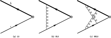
Figure 1: Typical Feynman diagrams for the QCD vertex function with the $\bar{b}c$ system up to two-loop order. The cross “$\bigoplus$” implies the insertion of the flavor-changing heavy quark scalar current.

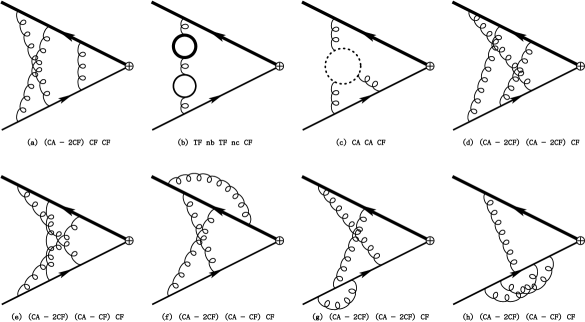
Figure 2: Typical Feynman diagrams labelled with the corresponding color factor for the QCD vertex function with the flavor-changing heavy quark scalar current at three-loop order. The cross “$\bigoplus$” implies the insertion of the scalar current. The thickest solid closed circle represents the bottom quark loop, and the other solid closed circle represents the charm quark loop. The dotted closed circle represents the ghost loop.

IV Results 

Following Refs. Feng:2022vvk ; Feng:2022ruy ; Sang:2022tnh , the dimensionless matching coefficient $\mathcal{C}_{s}$ for the flavor-changing scalar current involving the heavy bottom and charm quark can be decomposed as:

$$\mathcal{C}_{s}(\mu_{f},\mu,m_{b},m_{c}) = 1+\frac{\alpha_{s}^{\left(n_{l}\right)}\left(\mu\right)}{\pi}\mathcal{C}^{(1)}(x)+\left(\frac{\alpha_{s}^{\left(n_{l}\right)}\left(\mu\right)}{\pi}\right)^{2}\left(\mathcal{C}^{(1)}(x)\frac{\beta_{0}^{(n_{l})}}{4}\text{ln}\frac{\mu^{2}}{m_{b}m_{c}}+\frac{\tilde{\gamma}_{s}^{(2)}(x)}{2}\ln\frac{\mu_{f}^{2}}{m_{b}m_{c}}+\mathcal{C}^{(2)}(x)\right)$$ (14)

$$+\left(\frac{\alpha_{s}^{\left(n_{l}\right)}\left(\mu\right)}{\pi}\right)^{3}\Bigg{\{}\left(\frac{\mathcal{C}^{(1)}(x)}{16}\beta_{1}^{(n_{l})}+\frac{\mathcal{C}^{(2)}(x)}{2}\beta_{0}^{(n_{l})}\right)\text{ln}\frac{\mu^{2}}{m_{b}m_{c}}+\frac{\mathcal{C}^{(1)}(x)}{16}{\beta_{0}^{(n_{l})}}^{2}\ln^{2}\frac{\mu^{2}}{m_{b}m_{c}}$$

$$-\frac{1}{8}\left(\frac{d\tilde{\gamma}_{s}^{(3)}\left(x,\frac{\mu_{f}^{2}}{m_{b}m_{c}}\right)}{d\text{ln}\mu_{f}}+\beta_{0}^{(n_{l})}\tilde{\gamma}_{s}^{(2)}(x)\right)\ln^{2}\frac{\mu_{f}^{2}}{m_{b}m_{c}}+\frac{1}{2}\left(\mathcal{C}^{(1)}(x)\tilde{\gamma}_{s}^{(2)}(x)+\tilde{\gamma}_{s}^{(3)}\left(x,\frac{\mu_{f}^{2}}{m_{b}m_{c}}\right)\right)\ln\frac{\mu_{f}^{2}}{m_{b}m_{c}}$$

$$+\frac{\beta_{0}^{(n_{l})}}{4}\tilde{\gamma}_{s}^{(2)}(x)\ln\frac{\mu_{f}^{2}}{m_{b}m_{c}}\,\text{ln}\frac{\mu^{2}}{m_{b}m_{c}}+\mathcal{C}^{(3)}(x)\Bigg{\}}+\mathcal{O}\left(\alpha_{s}^{4}\right),$$

where the coefficients $\tilde{\gamma}_{s}^{(2)}(x)$ and $\tilde{\gamma}_{s}^{(3)}\left(x,\frac{\mu_{f}^{2}}{m_{b}m_{c}}\right)$ have been defined in Eqs. (6,7,8). The parameters $\mathcal{C}^{(i)}(x)(i=1,2,3)$ in above equation are independent of $\ln\mu$ and $\ln\mu_{f}$ and are the nontrivial parts of $\mathcal{C}_{s}$ at $\mathcal{O}\left(\alpha_{s}^{i}\right)$. It’s also well known that the coefficients $\mathcal{C}_{s}$ and $\mathcal{C}^{(i)}(x)$ satisfy the following symmetric replacements  Braaten:1995ej ; Hwang:1999fc ; Lee:2010ts ; Onishchenko:2003ui ; Chen:2015csa ; Feng:2022ruy ; Sang:2022tnh :

$$\mathcal{C}_{s}(\mu_{f},\mu,m_{b},m_{c}) = \mathcal{C}_{s}(\mu_{f},\mu,m_{c},m_{b})|_{n_{b}\leftrightarrow n_{c}},$$ (15)

$$\mathcal{C}^{(i)}(x) = \mathcal{C}^{(i)}\left(\frac{1}{x}\right)|_{n_{b}\leftrightarrow n_{c}}.$$ (16)

The one-loop QCD correction to $\mathcal{C}_{s}$, denoted by $\mathcal{C}^{(1)}(x)$, can be analytically achieved as:

$$\mathcal{C}^{(1)}(x)=\frac{3}{4}C_{F}\left(\frac{x-1}{x+1}\,\ln x-\frac{2}{3}\right).$$ (17)

The two-loop and three-loop matching coefficients in (14) are $\mathcal{C}^{(2)}(x)$ and $\mathcal{C}^{(3)}(x)$, which can be decomposed in terms of the different color/flavor structures by following the conventions as being used in Refs. Marquard:2014pea ; Beneke:2014qea ; Egner:2022jot ; Feng:2022vvk ; Feng:2022ruy ; Sang:2022tnh :

$$\mathcal{C}^{(2)}(x) = C_{F}^{2}\mathcal{C}_{FF}(x)+C_{F}C_{A}\mathcal{C}_{FA}(x)+C_{F}T_{F}n_{b}\mathcal{C}_{FB}(x)+C_{F}T_{F}n_{c}\mathcal{C}_{FC}(x)+C_{F}T_{F}n_{l}\mathcal{C}_{FL}(x),$$ (18)

$$\mathcal{C}^{(3)}(x) = C^{3}_{F}\,\mathcal{C}_{FFF}(x)+C^{2}_{F}\,C_{A}\,\mathcal{C}_{FFA}(x)+C_{A}^{2}C_{F}\,\mathcal{C}_{FAA}(x)+C^{2}_{F}T_{F}n_{l}\,\mathcal{C}_{FFL}(x)+C_{A}C_{F}T_{F}n_{l}\,\mathcal{C}_{FAL}(x)$$ (19)

$$+C_{F}T^{2}_{F}n_{l}\,n_{c}\,\mathcal{C}_{FCL}(x)+C_{F}T^{2}_{F}\,n_{l}n_{b}\,\mathcal{C}_{FBL}(x)+C_{F}T^{2}_{F}\,n^{2}_{l}\,\mathcal{C}_{FLL}(x)+C_{F}T_{F}^{2}\,n_{b}\,n_{c}\,\mathcal{C}_{FBC}(x)$$

$$+C^{2}_{F}T_{F}n_{c}\,\,\mathcal{C}_{FFC}(x)+C_{A}C_{F}T_{F}\,n_{c}\,\mathcal{C}_{FAC}(x)+C_{F}T^{2}_{F}\,n_{c}^{2}\,\mathcal{C}_{FCC}(x)$$

$$+C^{2}_{F}T_{F}\,n_{b}\,\mathcal{C}_{FFB}(x)+C_{A}C_{F}T_{F}\,n_{b}\,\mathcal{C}_{FAB}(x)+C_{F}T^{2}_{F}\,n_{b}^{2}\,\mathcal{C}_{FBB}(x).$$

Due to limited computing resources, we choose to calculate the matching coefficient $\mathcal{C}_{s}$ at three rational numerical points: the physical point $\{m_{b}=\frac{475}{100}\,\mathrm{GeV},m_{c}=\frac{150}{100}\,\mathrm{GeV}\}\left(i.e.,x=x_{0}=\frac{150}{475}\right)$, the check point $\{m_{b}=\frac{475}{100}\,\mathrm{GeV},m_{c}=\frac{475}{100}\times\frac{475}{150}\,\mathrm{GeV}\}\left(i.e.,x=\frac{475}{150}\right)$ and the equal mass point $\{m_{b}=\frac{475}{100}\,\mathrm{GeV},m_{c}=\frac{475}{100}\,\mathrm{GeV}\}\left(i.e.,x=1\right)$, respectively. The results $\mathcal{C}_{s}$ obtained at the physical point and the check point verify the symmetric features of $\mathcal{C}^{(i)}(x)$ in Eq. (16). Our results $\mathcal{C}_{s}$ obtained at the equal mass point $x=1$ are consistent with the known matching coefficient results $\mathcal{C}_{s}$ for the scalar current with the equal quark mass case in the previous literatures Egner:2022jot ; Kniehl:2006qw ; Piclum:2007an . To confirm our calculation, we have also applied the same calculation procedure to the evaluation of the three-loop matching coefficients $\mathcal{C}_{v}$, $\mathcal{C}_{p}$, $\mathcal{C}_{(a,0)}$ for the flavor-changing heavy quark vector current, the flavor-changing heavy quark pseudoscalar current, the zeroth component of the axial-vector current with the flavor-changing heavy quarks, respectively, where our results verify $\mathcal{C}_{p}\equiv\mathcal{C}_{(a,0)}$ and our results $\mathcal{C}_{v}$ and $\mathcal{C}_{(a,0)}$ agree with the known results in previous literature Kniehl:2006qw ; Piclum:2007an ; Marquard:2014pea ; Tao:2022qxa ; Egner:2022jot ; Feng:2022ruy ; Sang:2022tnh .

In the following, we will present the highly accurate numerical results of $\mathcal{C}^{(2)}(x)$ and $\mathcal{C}^{(3)}(x)$ at the physical heavy quark mass ratio $x=x_{0}=1.5/4.75$ with about 30-digit precision. The various components of ${\cal C}^{(2)}(x_{0})$ read:

$$\mathcal{C}_{FF}(x_{0}) = -6.96020737354849312657205418357,$$

$$\mathcal{C}_{FA}(x_{0}) = -4.12970820397051570036738297443,$$

$$\mathcal{C}_{FB}(x_{0}) = 0.048170796075386686136602545271,$$

$$\mathcal{C}_{FC}(x_{0}) = 0.268781876466689639100436656736,$$

$$\mathcal{C}_{FL}(x_{0}) = -0.363661393326874053432216153222.$$ (20)

And the various components of ${\cal C}^{(3)}(x_{0})$ read:

$$\mathcal{C}_{FFF}(x_{0}) = -12.6512824902497489841790999287,$$

$$\mathcal{C}_{FFA}(x_{0}) = -91.3076763843495687930187876995,$$

$$\mathcal{C}_{FAA}(x_{0}) = -67.2034246352357623358462321068,$$

$$\mathcal{C}_{FFL}(x_{0}) = 31.12323218543900065296825277243,$$

$$\mathcal{C}_{FAL}(x_{0}) = 19.49987491622541782889333507621,$$

$$\mathcal{C}_{FCL}(x_{0}) = -0.262383795777090819586462489511,$$

$$\mathcal{C}_{FBL}(x_{0}) = -0.0100054359359386271416783335057,$$

$$\mathcal{C}_{FLL}(x_{0}) = 0.3393017746199103339986949104357,$$

$$\mathcal{C}_{FBC}(x_{0}) = 0.0551829420149711792507691937024,$$

$$\mathcal{C}_{FFC}(x_{0}) = 4.4105666464862568415402096694718,$$

$$\mathcal{C}_{FAC}(x_{0}) = -0.6861454400278606762848799078670,$$

$$\mathcal{C}_{FCC}(x_{0}) = 0.09536045103106728669303211267177,$$

$$\mathcal{C}_{FFB}(x_{0}) = 1.1373781611175929139065523549900,$$

$$\mathcal{C}_{FAB}(x_{0}) = -0.318775996588438248091557753877,$$

$$\mathcal{C}_{FBB}(x_{0}) = 0.00994219408487397025982150577842.$$ (21)

From the numerical results in Eqs. (20,21), we find the dominant contributions in $\mathcal{C}^{(2)}(x_{0})$ and $\mathcal{C}^{(3)}(x_{0})$ come from the components corresponding to the color structures $C_{F}^{2}$, $C_{F}C_{A}$, $C_{F}^{2}C_{A}$ and $C_{F}C_{A}^{2}$, and the contributions from the bottom and charm quark loops are negligible.

Fixing the renormalization scale $\mu=m_{b}=4.75\mathrm{GeV}$, $m_{c}=1.5\mathrm{GeV}$, and setting the factorization scale $\mu_{f}=1\,\mathrm{GeV}$, Eq. (14) then reduces to

$$\mathcal{C}_{s}(x_{0}) = 1-0.06727332\left(\frac{\alpha_{s}^{\left(n_{l}=3\right)}(m_{b})}{\pi}\right)-12.41489\left(\frac{\alpha_{s}^{\left(n_{l}=3\right)}(m_{b})}{\pi}\right)^{2}$$ (22)

$$-930.1229\left(\frac{\alpha_{s}^{\left(n_{l}=3\right)}(m_{b})}{\pi}\right)^{3}+\mathcal{O}(\alpha_{s}^{4}).$$

With the values of $\alpha_{s}^{\left(n_{l}=3\right)}(\mu)$ calculated by the renormalization group running equation in Eq. (11), we investigate the renormalization scale dependence of the matching coefficient $\mathcal{C}_{s}$ for scalar current at LO, NLO, NNLO and N³LO accuracy in Fig. 3.

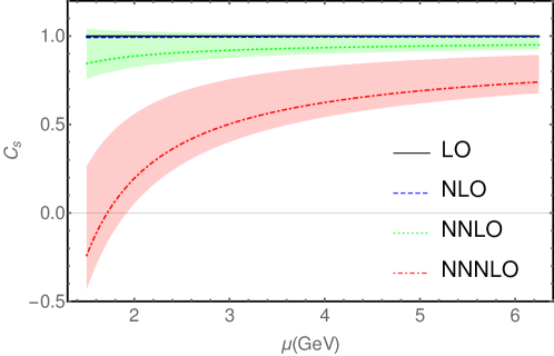
Figure 3: The renormalization scale dependence of the matching coefficient $\mathcal{C}_{s}$ at the LO, NLO, NNLO and N³LO accuracy. The central values of the matching coefficient $\mathcal{C}_{s}$ are calculated inputting the physical values with $\mu_{f}=1~{}\,\mathrm{GeV}$, $m_{b}=4.75\mathrm{GeV}$ and $m_{c}=1.5\mathrm{GeV}$. The error bands come from varying $\mu_{f}$ from 1.5 to 0.4 $\mathrm{GeV}$.

We also present our precise numerical results of the matching coefficient $\mathcal{C}_{s}$ for scalar current at LO, NLO , NNLO and N³LO in Tab. 1. The central values of the matching coefficient $\mathcal{C}_{s}$ are calculated by inputting the physical values with $\mu_{f}=1~{}\mathrm{GeV}$, $\mu=4.75\mathrm{GeV}$, $m_{b}=4.75\mathrm{GeV}$ and $m_{c}=1.5\mathrm{GeV}$. The errors are estimated by varying $\mu_{f}$ from 1.5 to 0.4 $\mathrm{GeV}$, $\mu$ from 6.25 to 3 $\mathrm{GeV}$, respectively.

Table 1: The values of the matching coefficient $\mathcal{C}_{s}$ for the flavor-changing heavy quark scalar current up to N³LO. For details, see the text.

	LO	NLO	NNLO	N3LO
$\mathcal{C}_{s}$	$1$	$0.99557^{-0+0.00037}_{+0-0.00082}$	$0.94186^{-0.03068+0.00873}_{+0.06933-0.02179}$	$0.67714^{-0.07379+0.06332}_{+0.18133-0.17414}$

From Fig. 3 and Tab.  1, one can find that the higher order QCD corrections have large influence compared with the NLO correction. Especially, the ${\cal O}(\alpha_{s}^{3})$ correction looks quite sizable, which confirms the breakdown of the convergence at ${\cal O}(\alpha_{s}^{3})$ for other heavy quark currents in previous literatures Egner:2022jot ; Feng:2022ruy ; Sang:2022tnh . Note that, at each truncated perturbative order, the matching coefficient $\mathcal{C}_{s}$ is renormalization-group invariant Feng:2022ruy ; Sang:2022tnh , e.g., at N³LO, $\mathcal{C}_{s}$ obeys the following renormalization-group running invariance:

$$\mathcal{C}_{s}^{\rm N^{3}LO}(\mu_{f},\mu,m_{b},m_{c})=\mathcal{C}_{s}^{\rm N^{3}LO}(\mu_{f},\mu_{0},m_{b},m_{c})+\mathcal{O}(\alpha_{s}^{4}),$$ (23)

where $\mathcal{C}_{s}^{\rm N^{3}LO}(\mu_{f},\mu,m_{b},m_{c})$ has dropped the $\mathcal{O}(\alpha_{s}^{4})$ terms in Eq. (14). Namely the scale-dependence of the N³LO matching coefficients rises from $\mathcal{O}(\alpha_{s}^{4})$, which is suppressed compared to lower-order. However, the scale-independence coefficients of $\alpha_{s}^{4}$ such as $\mathcal{C}^{(3)}(x)$ and $\ln\mu_{f}$, which come from the $\mathcal{O}(\alpha_{s}^{3})$ order in Eq. (14), are considerably large by aforementioned calculation within the framework of the NRQCD theory. These terms will lead to a significantly larger renormalization scale dependence at N³LO. From Fig. 3, we also find the NRQCD factorization scale $\mu_{f}$ has a large influence on the matching coefficient. When $\mu_{f}$ decreases, both the convergence of $\alpha_{s}$ expansion series and the independence of $\mu$ will be improved. The understanding of the observed large NNNLO corrections in this paper and the previous literatures Egner:2022jot ; Feng:2022ruy ; Sang:2022tnh is another important topic, which may be related to the higher order corrections to NRQCD long-distance nonperturbative matrix elements, higher order relativistic corrections and the resummation techniques. We will leave it in the future work.

V Summary 

In this paper, we have performed the $\rm N^{3}LO$ QCD corrections to the matching coefficient for the flavor-changing heavy quark scalar current involving the bottom and charm quark within the framework of the NRQCD effective theory. For the first time, we obtain the analytical expressions of the three-loop renormalization constant and the corresponding three-loop anomalous dimension of the NRQCD scalar current with different heavy quark mass $m_{b}$ and $m_{c}$. Meanwhile, the three-loop matching coefficient $C_{s}(\mu_{f},\mu,m_{b},m_{c})$ has also been obtained with high numerical accuracy, which is helpful to analyze the threshold behaviours when two different heavy quarks are close to each other. The obtained $\rm N^{3}LO$ QCD corrections are considerably large compared with lower-order corrections, and exhibit stronger dependence on the QCD renormalization scale and the NRQCD factorization scale at higher order, which suggests that higher order QCD corrections should be combined with other techniques in order to get a reliable prediction within the NRQCD effective theory.

- (1) G. T. Bodwin, E. Braaten and G. P. Lepage, Phys. Rev. D 51, 1125-1171 (1995) [erratum: Phys. Rev. D 55, 5853 (1997)].
- (2) E. Braaten and S. Fleming, Phys. Rev. D 52, 181-185 (1995).
- (3) D. S. Hwang and S. Kim, Phys. Rev. D 60, 034022 (1999).
- (4) J. Lee, W. Sang and S. Kim, JHEP 01, 113 (2011).
- (5) A. I. Onishchenko and O. L. Veretin, Eur. Phys. J. C 50, 801-808 (2007).
- (6) L. B. Chen and C. F. Qiao, Phys. Lett. B 748, 443-450 (2015).
- (7) F. Feng, Y. Jia, Z. Mo, J. Pan, W. L. Sang and J. Y. Zhang, [arXiv:2208.04302 [hep-ph]].
- (8) W. Tao, R. Zhu and Z. J. Xiao, Phys.Rev. D 107 (2023) in press. [arXiv:2209.15521 [hep-ph]].
- (9) W. L. Sang, H. F. Zhang and M. Z. Zhou, [arXiv:2210.02979 [hep-ph]].
- (10) B. A. Kniehl, A. Onishchenko, J. H. Piclum and M. Steinhauser, Phys. Lett. B 638, 209-213 (2006).
- (11) J. H. Piclum, doi:10.3204/DESY-THESIS-2007-014.
- (12) M. Egner, M. Fael, F. Lange, K. Schönwald and M. Steinhauser, Phys. Rev. D 105, 114007 (2022).
- (13) A. G. Grozin, P. Marquard, J. H. Piclum and M. Steinhauser, Nucl. Phys. B 789, 277-293 (2008).
- (14) D. J. Broadhurst and A. G. Grozin, Phys. Rev. D 52, 4082-4098 (1995).
- (15) P. Marquard, J. H. Piclum, D. Seidel and M. Steinhauser, Nucl. Phys. B 758, 144-160 (2006).
- (16) M. Egner, M. Fael, J. Piclum, K. Schoenwald and M. Steinhauser, Phys. Rev. D 104, 054033 (2021).
- (17) M. Beneke, A. Signer and V. A. Smirnov, Phys. Rev. Lett. 80, 2535-2538 (1998).
- (18) P. Marquard, J. H. Piclum, D. Seidel and M. Steinhauser, Phys. Lett. B 678, 269-275 (2009).
- (19) P. Marquard, J. H. Piclum, D. Seidel and M. Steinhauser, Phys. Rev. D 89, 034027 (2014).
- (20) B. A. Kniehl, A. A. Penin, M. Steinhauser and V. A. Smirnov, Phys. Rev. Lett. 90, 212001 (2003); [erratum: Phys. Rev. Lett. 91, 139903 (2003)].
- (21) L. B. Chen, J. Jiang and C. F. Qiao, JHEP 04, 080 (2018).
- (22) V. V. Kiselev and A. I. Onishchenko, [arXiv:hep-ph/9810283 [hep-ph]].
- (23) A. Czarnecki and K. Melnikov, Phys. Rev. Lett. 80, 2531-2534 (1998).
- (24) W. Tao, Z. J. Xiao and R. Zhu, Phys. Rev. D 105, 114026 (2022).
- (25) R. Zhu, Y. Ma, X. L. Han and Z. J. Xiao, Phys. Rev. D 95, 094012 (2017).
- (26) R. Zhu, Nucl. Phys. B 931, 359-382 (2018).
- (27) R. N. Lee, A. V. Smirnov, V. A. Smirnov and M. Steinhauser, JHEP 05, 187 (2018).
- (28) G. Bell, M. Beneke, T. Huber and X. Q. Li, Nucl. Phys. B 843, 143-176 (2011).
- (29) F. Feng, Y. Jia, Z. Mo, J. Pan, W. L. Sang and J. Y. Zhang, [arXiv:2207.14259 [hep-ph]].
- (30) S. Bekavac, A. Grozin, D. Seidel and M. Steinhauser, JHEP 10, 006 (2007).
- (31) P. Marquard, A. V. Smirnov, V. A. Smirnov, M. Steinhauser and D. Wellmann, Phys. Rev. D 94, 074025 (2016).
- (32) M. Fael, K. Schönwald and M. Steinhauser, JHEP 10, 087 (2020).
- (33) C. Duhr and F. Dulat, JHEP 08, 135 (2019).
- (34) A. Mitov and S. Moch, JHEP 05, 001 (2007).
- (35) K. G. Chetyrkin, B. A. Kniehl and M. Steinhauser, Nucl. Phys. B 510, 61 (1998).
- (36) T. van Ritbergen, J. A. M. Vermaseren and S. A. Larin, Phys. Lett. B 400, 379 (1997).
- (37) Ferguson, H., Bailey, D. and Arno, S., Mathematics Of Computation 68, 351 (1999).
- (38) M. Abramowitz and I. Stegun, Handbook of Mathematical Functions: With Formulas, Graphs, and Mathematical Tables. Dover Publications, 1964.
- (39) S. Groote, J. G. Korner and O. I. Yakovlev, Phys. Rev. D 54, 3447 (1996).
- (40) J. Henn, A. V. Smirnov, V. A. Smirnov and M. Steinhauser, JHEP 01, 074 (2017).
- (41) M. Fael, F. Lange, K. Schönwald and M. Steinhauser, Phys. Rev. D 106, 034029 (2022).
- (42) A. Grozin, J. M. Henn, G. P. Korchemsky and P. Marquard, JHEP 01, 140 (2016).
- (43) M. A. Özcelik, tel-03362708.
- (44) K. G. Chetyrkin, J. H. Kuhn and C. Sturm, Nucl. Phys. B 744, 121 (2006).
- (45) W. Bernreuther and W. Wetzel, Nucl. Phys. B 197, 228 (1982); [erratum: Nucl. Phys. B 513, 758 (1998)].
- (46) P. Bärnreuther, M. Czakon and P. Fiedler, JHEP 02, 078 (2014).
- (47) S. Abreu, M. Becchetti, C. Duhr and M. A. Ozcelik, [arXiv:2211.08838 [hep-ph]].
- (48) K. G. Chetyrkin, J. H. Kuhn and M. Steinhauser, Comput. Phys. Commun. 133, 43 (2000).
- (49) B. Schmidt and M. Steinhauser, Comput. Phys. Commun. 183, 1845 (2012).
- (50) A. Deur, S. J. Brodsky and G. F. de Teramond, Nucl. Phys. 90, 1 (2016).
- (51) F. Herren and M. Steinhauser, Comput. Phys. Commun. 224, 333 (2018).
- (52) V. Shtabovenko, R. Mertig and F. Orellana, Comput. Phys. Commun. 256, 107478 (2020).
- (53) F. Feng, Comput. Phys. Commun. 183, 2158 (2012).
- (54) A. V. Smirnov and F. S. Chuharev, Comput. Phys. Commun. 247, 106877 (2020).
- (55) J. Klappert, F. Lange, P. Maierhöfer and J. Usovitsch, Comput. Phys. Commun. 266, 108024 (2021).
- (56) T. Peraro, JHEP 07, 031 (2019).
- (57) K. G. Chetyrkin and F. V. Tkachov, Nucl. Phys. B 192, 159-204 (1981).
- (58) M. Fael, K. Schönwald and M. Steinhauser, Phys. Rev. D 103, 014005 (2021).
- (59) X. Liu and Y. Q. Ma, Comput. Phys. Commun. 283, 108565 (2023).
- (60) X. Liu, Y. Q. Ma and C. Y. Wang, Phys. Lett. B 779, 353 (2018).
- (61) R. Bonciani and A. Ferroglia, JHEP 11, 065 (2008).
- (62) A. I. Davydychev, P. Osland and O. V. Tarasov, Phys. Rev. D 58, 036007 (1998).
- (63) T. de Oliveira, D. Harnett, A. Palameta and T. G. Steele, [arXiv:2208.12363 [hep-ph]].
- (64) C. Brønnum-Hansen and C. Y. Wang, JHEP 05, 244 (2021).
- (65) X. Chen, X. Guan, C. Q. He, X. Liu and Y. Q. Ma, [arXiv:2209.14259 [hep-ph]].
- (66) X. Chen, X. Guan, C. Q. He, Z. Li, X. Liu and Y. Q. Ma, [arXiv:2209.14953 [hep-ph]].
- (67) M. Beneke, Y. Kiyo, P. Marquard, A. Penin, J. Piclum, D. Seidel and M. Steinhauser, Phys. Rev. Lett. 112, 151801 (2014).