Infrared behavior in tame hyperbolizable two-field models

Abstract

We discuss the behavior of cosmological curves and their first order infrared approximants near critical ends of the scalar manifold $\Sigma$ and near interior critical points of the scalar potential for tame hyperbolizable two-field cosmological models by determining the universal forms of the asymptotic gradient flow of the classical effective potential with respect to the uniformizing metric near all these points and ends. We compare the asymptotic behavior of gradient flow curves with numerical results for cosmological curves.

1 Introduction

Two-field cosmological models provide the simplest testing ground for multifield cosmological dynamics. The latter are of great importance for connecting cosmology with fundamental theories of gravity and matter, since the effective description of generic string and M-theory compactifications contains many moduli fields. In particular, multifield models are crucial in cosmological applications of the swampland program [1, 2, 3, 4], as pointed out for example in [5, 6, 7], and may also allow for a unified description of inflation, dark matter and dark energy [8].

A two-field cosmological model is parameterized by a connected borderless smooth surface $\Sigma$ (the target manifold of the scalar fields) endowed with a Riemannian metric $\mathcal{G}$ and a scalar potential $\Phi$ which is a smooth function defined on $\Sigma$. We assume that $\Phi$ is positive everywhere. In [9], we used a dynamical RG (renormalization group) flow analysis and the uniformization theorem of Poincaré to show that two-field models whose scalar field metric $\mathcal{G}$ has constant Gaussian curvature $K$ equal to $-1$, $0$ or $+1$ give distinguished representatives for the IR (infrared) universality classes of all two-field cosmological models. Hyperbolizable two-field models (which are defined as those models for which $K=-1$) comprise all two-field models whose target is of general type as well as those models whose target is exceptional (i.e diffeomorphic with $\mathbb{R}^{2}$, the annulus $\mathrm{A}^{2}$ or the Möbius strip $\mathrm{M}^{2}$) and for which the metric belongs to a hyperbolizable conformal class. The uniformized form of a hyperbolizable model is a two-field generalized $\alpha$-attractor model in the sense of [10]. Some aspects of such models were investigated previously in [11, 12, 13, 14, 17, 15, 16] (see [18, 19, 20, 21] for brief reviews).

The infrared behavior of a tractable class of hyperbolizable two-field models was studied in [22], work which we summarize here together with a brief announcement of further results. We will assume that the target manifold $\Sigma$ is oriented and topologically finite in the sense that it has finitely-generated fundamental group. When $\Sigma$ is non-compact, this condition insures that it has a finite number of Freudenthal ends [23] and that its end compactification $\widehat{\Sigma}$ is a smooth and oriented compact surface. Thus $\Sigma$ is recovered from $\widehat{\Sigma}$ by removing a finite number of points. We also assume that the scalar potential $\Phi$ admits a smooth extension ${\hat{\Phi}}$ to $\widehat{\Sigma}$ which is a strictly-positive Morse function defined on $\widehat{\Sigma}$. A two-field cosmological model is called tame when these conditions are satisfied. Thus tame hyperbolizable two-field cosmological models are those classical two-field models whose scalar manifold is a connected, oriented and topologically finite hyperbolizable Riemann surface $(\Sigma,\mathcal{G})$ and whose scalar potential $\Phi$ admits a positive and Morse extension to the end compactification of $\Sigma$.

Notations and conventions.

All surfaces $\Sigma$ considered here are connected, smooth, Hausdorff and paracompact. If $V$ is a smooth real-valued function defined on $\Sigma$, we denote by:

$$\mathrm{Crit}V\stackrel{{\scriptstyle{\rm def.}}}{{=}}\{c\in\Sigma|(\mathrm{d}V)(c)=0\}$$

the set of its critical points. For any $c\in\mathrm{Crit}V$, we denote by $\mathrm{Hess}(V)(c)$ the Hessian of $V$ at $c$, which is a well-defined and coordinate independent symmetric bilinear form on the tangent space $T_{c}\Sigma$. Given a metric $\mathcal{G}$ on $\Sigma$, we define the covariant Hessian tensor of $V$ relative to $\mathcal{G}$ by:

$$\mathrm{Hess}_{\mathcal{G}}(V)\stackrel{{\scriptstyle{\rm def.}}}{{=}}\nabla\mathrm{d}V~{}~{},$$

where $\nabla$ is the Levi-Civita connection of $\mathcal{G}$. This symmetric tensor has the following local expression in coordinates $(x^{1},x^{2})$ on $\Sigma$:

$$\mathrm{Hess}_{\mathcal{G}}(V)=(\partial_{i}\partial_{j}-\Gamma^{k}_{ij}(x)\partial_{k})V\mathrm{d}x^{i}\otimes\mathrm{d}x^{j}~{}~{},$$

where $\Gamma^{k}_{ij}(x)$ are the Christoffel symbols of $\mathcal{G}$. Recall that a critical point $c$ of $V$ is called nondegenerate if $\mathrm{Hess}_{\mathcal{G}}(V)(c)$ is a non-degenerate bilinear form. When $V$ is a Morse function (i.e. has only non-degenerate critical points), the set $\mathrm{Crit}V$ is discrete. We denote by $\widehat{\Sigma}$ the end compactification of $\Sigma$, which is a compact Hausdorff topological space containing $\Sigma$. In the topologically finite case, the surface $\Sigma$ has a finite number of Freudenthal ends and $\widehat{\Sigma}$ is a smooth compact surface. In this situation, we say that $V$ is globally well-behaved on $\Sigma$ if it admits a smooth extension $\widehat{V}$ to $\widehat{\Sigma}$. A metric $\mathcal{G}$ on $\Sigma$ is called hyperbolic if it is complete and of constant Gaussian curvature $K=-1$.

2 Hyperbolizable two-field models

Let us recall the global description of two-field cosmological models through a second order geometric ODE and the first order infrared approximation introduced in [9]. Such a model is parameterized by the rescaled Planck mass $M_{0}\stackrel{{\scriptstyle{\rm def.}}}{{=}}M\sqrt{\frac{2}{3}}$ (where $M$ is the reduced Planck mass) and by its scalar triple $(\Sigma,\mathcal{G},\Phi)$, where $\Sigma$ is the target manifold for the scalar fields (a generally non-compact borderless connected surface), $\mathcal{G}$ is the scalar field metric and $\Phi$ is the scalar potential. To ensure conservation of energy, one requires that $\mathcal{G}$ is complete. For simplicity, we also assume that $\Phi$ is strictly positive.

When neglecting fluctuations, the scalar field $\varphi:\mathbb{R}\rightarrow\Sigma$ coupled to the metric of a Friedmann-Lemaître-Robertson-Walker (FLRW) space satisfies the cosmological equation (see (1.4) in [22]):

$$\nabla_{t}\dot{\varphi}(t)+\frac{1}{M_{0}}\left[||\dot{\varphi}(t)||_{\mathcal{G}}^{2}+2\Phi(\varphi(t))\right]^{1/2}\dot{\varphi}(t)+(\mathrm{grad}_{\mathcal{G}}\Phi)(\varphi(t))=0~{}~{}.$$ (1)

Proposition 2.1.

The IR behavior (in the sense of [9]) of the cosmological flow of a two-field model with scalar triple $(\Sigma,\mathcal{G},\Phi)$ and rescaled Planck mass $M_{0}$ is described by the gradient flow of the scalar triple $(\Sigma,G,V)$, where $G$ is the uniformizing metric of $\mathcal{G}$ and $V\stackrel{{\scriptstyle{\rm def.}}}{{=}}M_{0}\sqrt{2\Phi}$ is the classical effective scalar potential of the model.

Hence the IR behavior is described by the gradient flow equation:

$$\dot{\varphi}_{\mathrm{IR}}(t)+(\mathrm{grad}_{G}{V})(\varphi_{\mathrm{IR}}(t))=0~{}.$$ (2)

The first order IR approximants of cosmological orbits for the model $(M_{0},\Sigma,\mathcal{G},\Phi)$ coincide with those of the model $(M_{0},\Sigma,G,\Phi)$. Moreover, these approximants coincide with the gradient flow orbits of $(\Sigma,G,V)$. In particular, the IR universality classes defined in [9] depend only on the scalar triple $(\Sigma,G,V)$. This allows for systematic studies of two-field cosmological models belonging to a fixed IR universality class by using the infrared expansion of cosmological curves, the first order of which is given by the gradient flow of the classical effective potential $V$ on the geometrically finite hyperbolic surface $(\Sigma,G)$. Since the future limit points of cosmological curves and of the gradient flow curves of $(\Sigma,G,V)$ are critical points of $\Phi$ or Freudenthal ends of $\Sigma$, the asymptotic behavior of such curves for late cosmological times is determined by the form of $G$ and $V$ near such points.

2.1 The hyperbolic metric $G$ in the vicinity of an end

In this subsection, we recall the form of the hyperbolic metric $G$ in a canonical vicinity of an end and extract its asymptotic behavior near each type of end.

Any end ${\bf e}$ of $\Sigma$ admits an open neighborhood $U_{\bf e}\subset\widehat{\Sigma}$ diffeomorphic with a disk such that there exist semigeodesic polar coordinates $(r,\theta)\in\mathbb{R}_{>0}\times\mathrm{S}^{1}$ defined on $\dot{U}_{\bf e}\stackrel{{\scriptstyle{\rm def.}}}{{=}}U_{\bf e}\setminus\{{\bf e}\}\subset\Sigma$ in which the metric $G$ has the canonical form:

$$\mathrm{d}s_{G}^{2}|_{\dot{U}_{\bf e}}=\mathrm{d}r^{2}+f_{\bf e}(r)\mathrm{d}\theta^{2}~{}~{},$$

$$f_{\bf e}(r)=\left\{\begin{array}[]{ll}\sinh^{2}(r)&\mbox{if}~{}{\bf e}=\mathrm{plane~{}end}\\ \frac{1}{(2\pi)^{2}}e^{2r}&\mbox{if}~{}{\bf e}=\mathrm{horn~{}end}\\ \frac{\ell^{2}}{(2\pi)^{2}}\cosh^{2}(r)&\mbox{if}~{}{\bf e}=\mathrm{funnel~{}end~{}of~{}circumference}~{}\ell>0\\ \frac{1}{(2\pi)^{2}}e^{-2r}&\mbox{if}~{}{\bf e}=\mathrm{cusp~{}end}\end{array}\right.~{}~{}.$$

The end corresponds to $r\!\rightarrow\!\infty$. Setting $\omega\!\stackrel{{\scriptstyle{\rm def.}}}{{=}}\!\frac{1}{r}$, the metric in canonical polar coordinates $(\omega,\theta)$ is:

$$\mathrm{d}s_{G}^{2}|_{\dot{U}_{\bf e}}=\frac{\mathrm{d}\omega^{2}}{\omega^{4}}+f_{\bf e}(1/\omega)\mathrm{d}\theta^{2}~{}~{},$$

where:

$$f_{\bf e}(1/\omega)={\tilde{c}}_{\bf e}e^{\frac{2\varepsilon_{\bf e}}{\omega}}\left[1+\mathrm{O}\left(e^{-\frac{2}{\omega}}\right)\right]~{}~{}\mathrm{for}~{}~{}\omega\to 0~{}~{},$$ (3)

with:

$${\tilde{c}}_{\bf e}=\left\{\begin{array}[]{ll}\frac{1}{4}&\mbox{if}~{}{\bf e}=\mathrm{plane~{}end}\\ \frac{1}{(2\pi)^{2}}&\mbox{if}~{}{\bf e}=\mathrm{horn~{}end}\\ \frac{\ell^{2}}{(4\pi)^{2}}&\mbox{if}~{}{\bf e}=\mathrm{funnel~{}end~{}of~{}circumference}~{}\ell>0\\ \frac{1}{(2\pi)^{2}}&\mbox{if}~{}{\bf e}=\mathrm{cusp~{}end}\end{array}\right.$$

$$\varepsilon_{\bf e}=\left\{\begin{array}[]{ll}+1&\mbox{if }~{}{\bf e}=\mathrm{flaring~{}(i.e.~{}plane,~{}horn~{}or~{}funnel)~{}end}\\ -1&\mbox{if }~{}{\bf e}=\mathrm{cusp~{}end}\end{array}\right.$$

The term $\mathrm{O}\left(e^{-\frac{2}{\omega}}\right)$ in (3) vanishes identically when ${\bf e}$ is a cusp or horn end. In particular, the constants ${\tilde{c}}_{\bf e}$ and $\epsilon_{\bf e}$ determine the leading asymptotic behavior of the hyperbolic metric $G$ near ${\bf e}$.

The gradient flow equations of $(\dot{U}_{\bf e},G|_{\dot{U}_{\bf e}},V|_{\dot{U}_{\bf e}})$ read:

$$\frac{\mathrm{d}\omega}{\mathrm{d}q}=-(\mathrm{grad}V)^{\omega}\simeq-\omega^{4}\partial_{\omega}V~{}~{}$$

$$\frac{\mathrm{d}\theta}{\mathrm{d}q}=-(\mathrm{grad}V)^{\theta}\simeq-\frac{1}{{\tilde{c}}_{\bf e}}e^{-\frac{2\epsilon_{\bf e}}{\omega}}\partial_{\theta}V~{}~{}.$$ (6)

We studied these equations in [22] for all ends of $\Sigma$. Below, we summarize the results for critical ends (see op. cit. for the noncritical ends).

Recall that $V$ is globally well-behaved and $\widehat{V}$ is Morse on $\widehat{\Sigma}$. Together with the formulas above, this implies that $(\mathrm{grad}_{G}V)^{\omega}$ tends to zero at all ends while $(\mathrm{grad}_{G}V)^{\theta}$ tends to zero exponentially at flaring (i.e. non-cusp) ends and to infinity at cusp ends. On the other hand, we have:

$$||\mathrm{grad}_{G}V||^{2}=||\mathrm{d}V||^{2}=\frac{1}{\omega^{4}}(\partial_{\omega}V)^{2}+f_{\bf e}(1/\omega)(\partial_{\theta}V)^{2}\approx\frac{1}{\omega^{4}}(\partial_{\omega}V)^{2}+{\tilde{c}}_{\bf e}e^{\frac{2\epsilon_{\bf e}}{\omega}}(\partial_{\theta}V)^{2}~{}~{}.$$

Thus $||\mathrm{grad}_{G}V||$ tends to infinity at all ends.

2.2 Principal canonical coordinates centered at an end ${\bf e}$

Definition 2.2.

A canonical Cartesian coordinate system $(x,y)$ for $(\Sigma,G)$ centered at the critical end ${\bf e}$ is called principal for $V$ if the tangent vectors $\epsilon_{x}=\frac{\partial}{\partial x}\big{|}_{\bf e}$ and $\epsilon_{y}=\frac{\partial}{\partial y}\big{|}_{\bf e}$ form a principal basis for $V$ at ${\bf e}$.

Canonical Cartesian coordinates $(x,y)$ centered at ${\bf e}$ are given by:

$$x=\omega\cos\theta=\frac{1}{r}\cos\theta~{}~{}~{},~{}~{}~{}y=\omega\sin\theta=\frac{1}{r}\sin\theta~{}.$$

In such coordinates, the end ${\bf e}$ corresponds to $\omega=0$, i.e. $(x,y)=(0,0)$. The Taylor expansion of $\widehat{V}$ at ${\bf e}$ in principal Cartesian coordinates $(x,y)$ centered at ${\bf e}$ and in associated polar coordinates $(\omega,\theta)$ reads:

$$\widehat{V}_{\bf e}(x,y)\! = \widehat{V}({\bf e})+\frac{1}{2}\!\left[\lambda_{1}({\bf e})x^{2}\!+\!\lambda_{2}({\bf e})y^{2}\right]+\mathrm{O}((x^{2}+y^{2})^{\frac{3}{2}})~{},$$

$$\!\!\widehat{V}_{\bf e}(\omega,\theta)\! = \!\widehat{V}({\bf e})+\frac{1}{2}\omega^{2}\!\left[\lambda_{1}({\bf e})\cos^{2}\theta\!+\!\lambda_{2}({\bf e})\sin^{2}\theta\right]+\mathrm{O}(\omega^{3})~{},$$ (7)

where $\omega=\sqrt{x^{2}+y^{2}}$, $\theta=\arg(x+\mathbf{i}y)$ and the real numbers $\lambda_{1}({\bf e})$ and $\lambda_{2}({\bf e})$ are the principal values of the Hessian of $\widehat{V}({\bf e})$. When $\lambda_{1}$ and $\lambda_{2}$ do not both vanish, it is convenient to define:

Definition 2.3.

The critical modulus of $(\Sigma,\!G,\!V)$ at the critical end ${\bf e}$ is the ratio:

$$\beta_{\bf e}\stackrel{{\scriptstyle{\rm def.}}}{{=}}\frac{\lambda_{1}({\bf e})}{\lambda_{2}({\bf e})}\in[-1,1]\setminus\{0\}~{}~{},$$

where $\lambda_{1}({\bf e})$ and $\lambda_{2}({\bf e})$ are the principal values of $(\Sigma,G,V)$ at ${\bf e}$.

Definition 2.4.

The characteristic signs of $(\Sigma,G,V)$ at ${\bf e}$ are:

$$\varepsilon_{i}({\bf e})\stackrel{{\scriptstyle{\rm def.}}}{{=}}\mathrm{sign}(\lambda_{i}({\bf e}))\in\{-1,1\}~{}~{}(i=1,2)~{}~{}.$$

The extended scalar potential ${\hat{\Phi}}$ of the canonical model can be recovered from the extended classical effective potential as:

$${\hat{\Phi}}=\frac{1}{2M_{0}^{2}}\widehat{V}^{2}\approx\frac{{\bar{\lambda}}_{2}({\bf e})^{2}}{2}\left[\hat{\bar{V}}({\bf e})+\frac{1}{2}\omega^{2}(\beta_{\bf e}\cos^{2}\theta+\sin^{2}\theta)\right]^{2}~{},$$ (8)

where we defined

$${\bar{\lambda}}_{2}({\bf e})\stackrel{{\scriptstyle{\rm def.}}}{{=}}\frac{\lambda_{2}({\bf e})}{M_{0}}~{}~{},~{}~{}{\hat{\bar{V}}}({\bf e})\stackrel{{\scriptstyle{\rm def.}}}{{=}}\frac{{\hat{V}}({\bf e})}{\lambda_{2}({\bf e})}~{}~{}.$$

Solving the gradient flow equation (2) of $V$ relative to $G$ with the approximations (3) and (2.2) for $\theta\not\in\{0,\frac{\pi}{2},\pi,\frac{3\pi}{2}\}$ shows that the unoriented gradient flow orbits of $V$ around the end ${\bf e}$ have implicit equation:

$$\frac{1}{4}[\lambda_{1}({\bf e})-\lambda_{2}({\bf e})]\,\Gamma_{2}\!\left(\frac{2\varepsilon_{\bf e}}{\omega}\right)=A+{\tilde{c}}_{\bf e}\left[\,\lambda_{1}({\bf e})\log|\sin\theta|-\lambda_{2}({\bf e})\log|\cos\theta|\,\right]~{}~{},$$ (9)

where $\Gamma_{2}$ is the lower incomplete Gamma function of order $2$ and $A$ is an integration constant.

Below, we compare graphically (making certain choices for $\beta$) the unoriented gradient flow orbits given implicitely by equation (9) to the orbits of IR optimal cosmological curves, defined as those solutions $\varphi$ of the cosmological equation (1) which satisfy $\dot{\varphi}(0)=-(\mathrm{grad}_{G}V)(\varphi(0))$.

2.3 The IR behavior near critical plane ends

Figure 1 bellow gives the unoriented gradient flow orbits for certain choices of $\beta$, while Figure 2 gives the numerically computed orbits of the IR optimal cosmological curves for the same choices of $\beta$ and various other assumptions mentioned in the description.

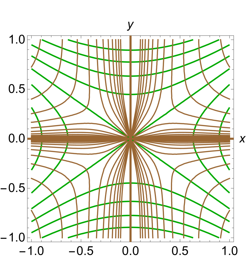
(a) For $\beta_{\bf e}=-0.5$

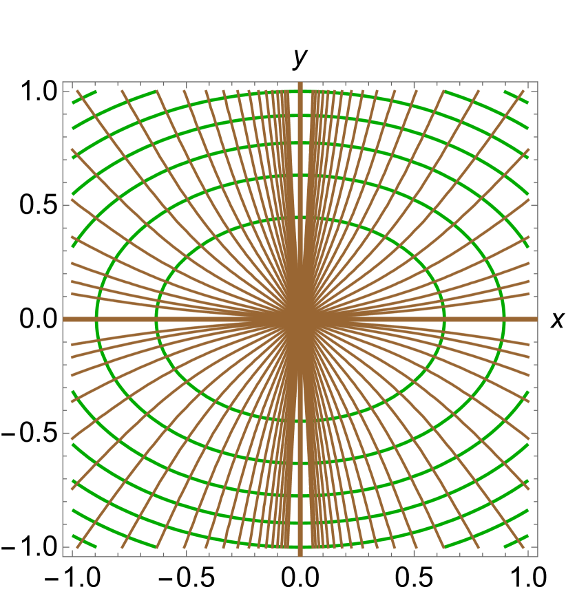
(b) For $\beta_{\bf e}=0.5$

Figure 1: Gradient flow orbits of $V$ (shown in brown) and level sets of $V$ (shown in green) near a critical plane end ${\bf e}$, drawn in principal Cartesian canonical coordinates centered at ${\bf e}$ for two values of $\beta_{\bf e}$.

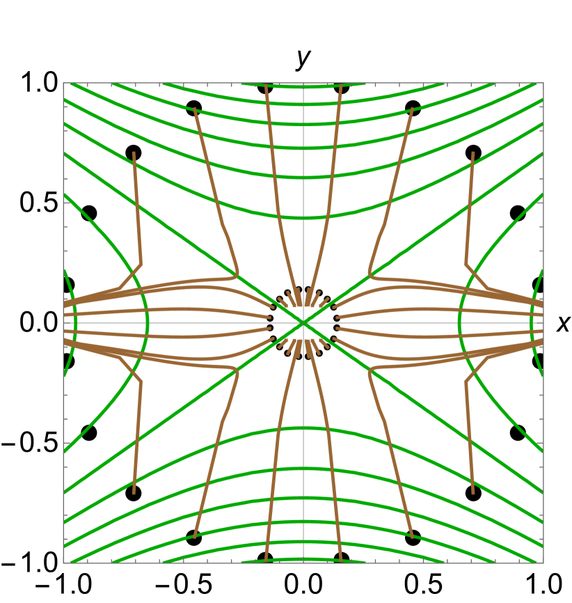
(a) For $\beta_{\bf e}=-0.5$

y

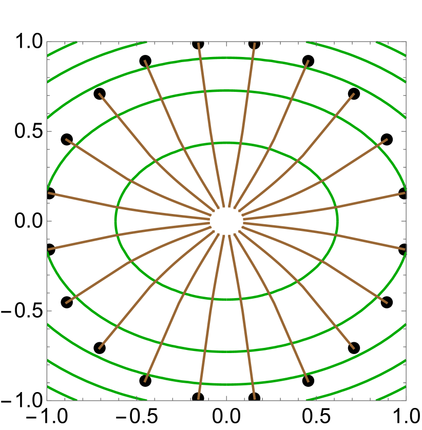
(b) For $\beta_{\bf e}=0.5$

Figure 2: Numerically computed infrared optimal cosmological orbits of the canonical model (shown in brown) and level sets of ${\hat{\Phi}}$ (shown in green) near a critical plane end ${\bf e}$, drawn in principal canonical Cartesian coordinates centered at ${\bf e}$ for two values of $\beta_{\bf e}$. We took ${\bar{\lambda}}_{2}({\bf e})=1$, ${\hat{\bar{V}}}({\bf e})=1$ and $M_{0}=1$. The initial point of each orbit, i.e. $\varphi(0)$, is shown as a black dot.

2.4 The IR behavior near critical horn ends

We graphically compare Figure 3 bellow, which gives the unoriented gradient flow orbits near critical horn ends, with Figure 4 which shows some numerically computed orbits of the IR optimal cosmological curves near critical horn ends. The comparison is done for certain choices of $\beta$.

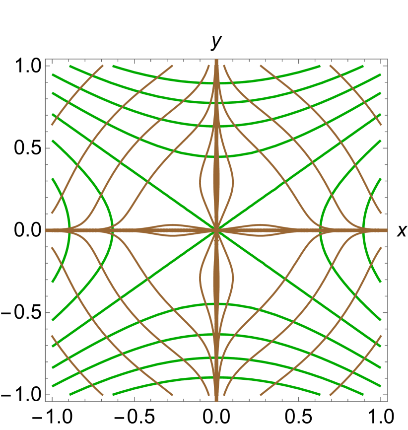
(a) For $\beta_{\bf e}=-0.5$.

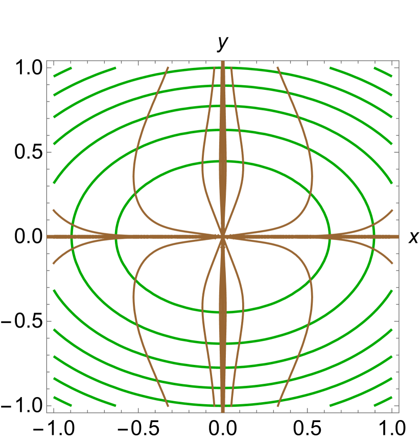
(b) For $\beta_{\bf e}=0.5$.

Figure 3: Gradient flow orbits of $V$ (shown in brown) and level sets of $V$ (shown in green) near a critical horn end ${\bf e}$, drawn in principal Cartesian canonical coordinates centered at ${\bf e}$ for two values of $\beta_{\bf e}$.

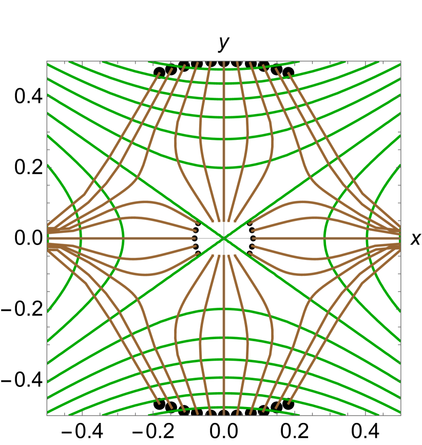
(a) For $\beta_{\bf e}=-0.5$.

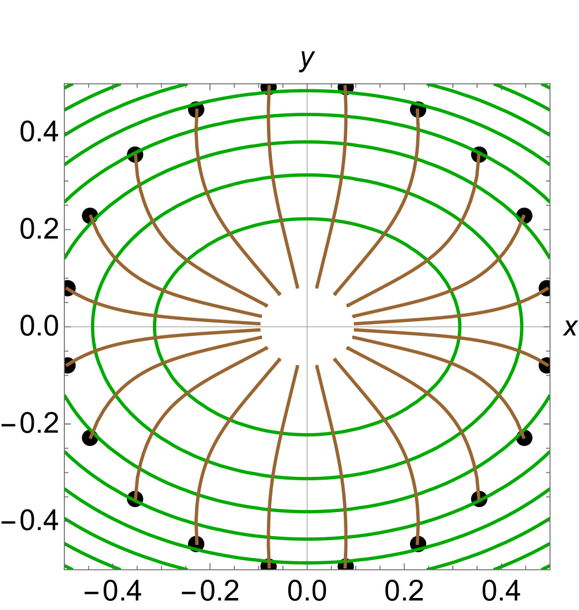
(b) For $\beta_{\bf e}=0.5$.

Figure 4: Numerically computed infrared optimal cosmological orbits of the canonical model (shown in brown) and level sets of ${\hat{\Phi}}$ (shown in green) near a critical horn end ${\bf e}$, drawn in principal canonical Cartesian coordinates centered at ${\bf e}$ for two values of $\beta_{\bf e}$. We took ${\bar{\lambda}}_{2}({\bf e})=1$, ${\hat{\bar{V}}}({\bf e})=1$ and $M_{0}=1$. The initial point $\varphi(0)$ of each orbit is shown as a black dot.

2.5 The IR behavior near critical funnel ends

We visually compare below Figure 5, which gives the unoriented gradient flow orbits near critical funnel ends, with Figure 6, which shows some numerically computed orbits of the IR optimal cosmological curves near critical funnel ends.

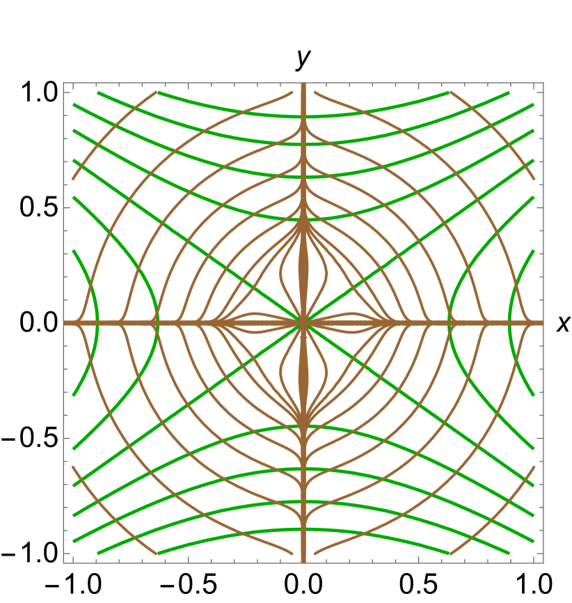
(a) For $\beta_{\bf e}=-0.5$.

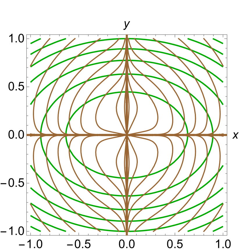
(b) For $\beta_{\bf e}=0.5$.

Figure 5: Gradient flow orbits of $V$ (shown in brown) and level sets of $V$ (shown in green) near a critical funnel end ${\bf e}$ of circumference $\ell=1$, drawn in principal Cartesian canonical coordinates centered at ${\bf e}$ for two values of $\beta_{\bf e}$.

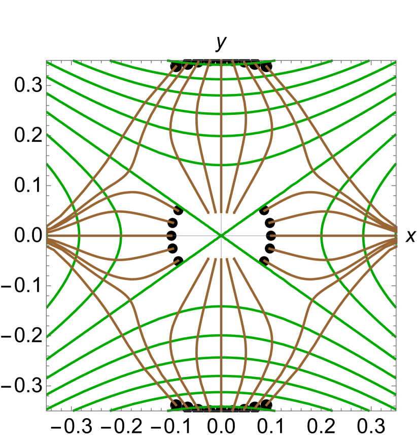
(a) For $\beta_{\bf e}=-0.5$.

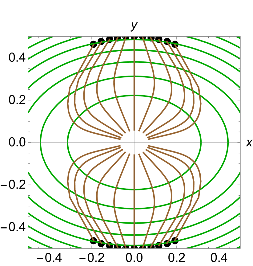
(b) For $\beta_{\bf e}=0.5$.

Figure 6: Numerically computed infrared optimal cosmological orbits of the canonical model (shown in brown) and level sets of ${\hat{\Phi}}$ (shown in green) near a critical funnel end ${\bf e}$ of circumference $\ell=1$, drawn in principal canonical coordinates centered at ${\bf e}$ for two values of $\beta_{\bf e}$. We took ${\bar{\lambda}}_{2}({\bf e})=1$, ${\hat{\bar{V}}}({\bf e})=1$ and $M_{0}=1$. The initial point $\varphi(0)$ of each orbit is shown as a black dot.

2.6 The IR behavior near critical cusp ends

By graphically comparing Figure 7, which gives some unoriented gradient flow orbits near critical cusp ends, and Figure 8, which shows some numerically computed orbits of the IR optimal cosmological curves near critical cusp ends, one can assume that higher order corrections are needed in the IR expansion to get better approximants for the cusp.

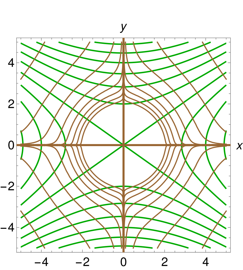
(a) For $\beta_{\bf e}=-0.5$.

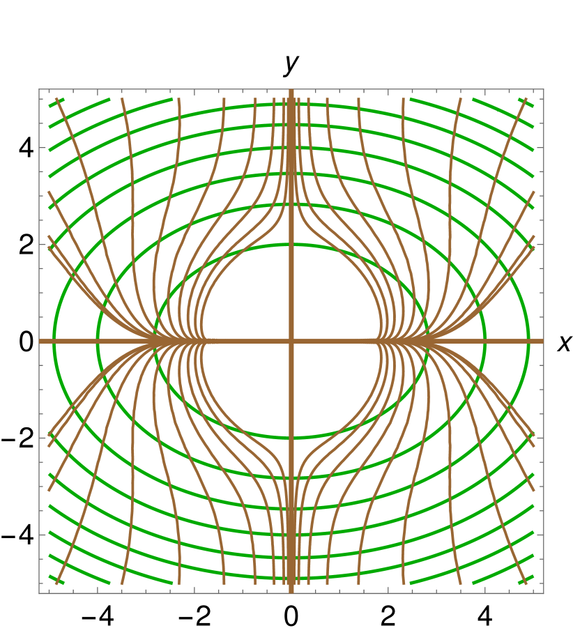
(b) For $\beta_{\bf e}=0.5$.

Figure 7: Gradient flow orbits of $V$ (shown in brown) and level sets of $V$ (shown in green) near a critical cusp end ${\bf e}$, drawn in principal Cartesian canonical coordinates centered at ${\bf e}$ for two values of $\beta_{\bf e}$.

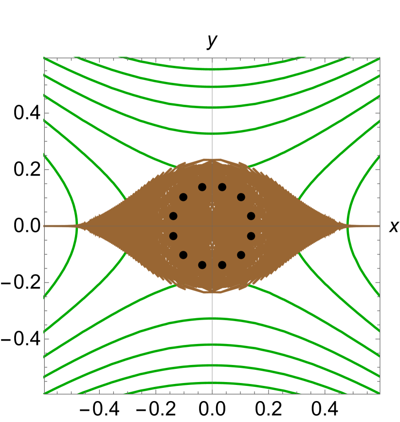
(a) For $\beta_{\bf e}=-0.5$.

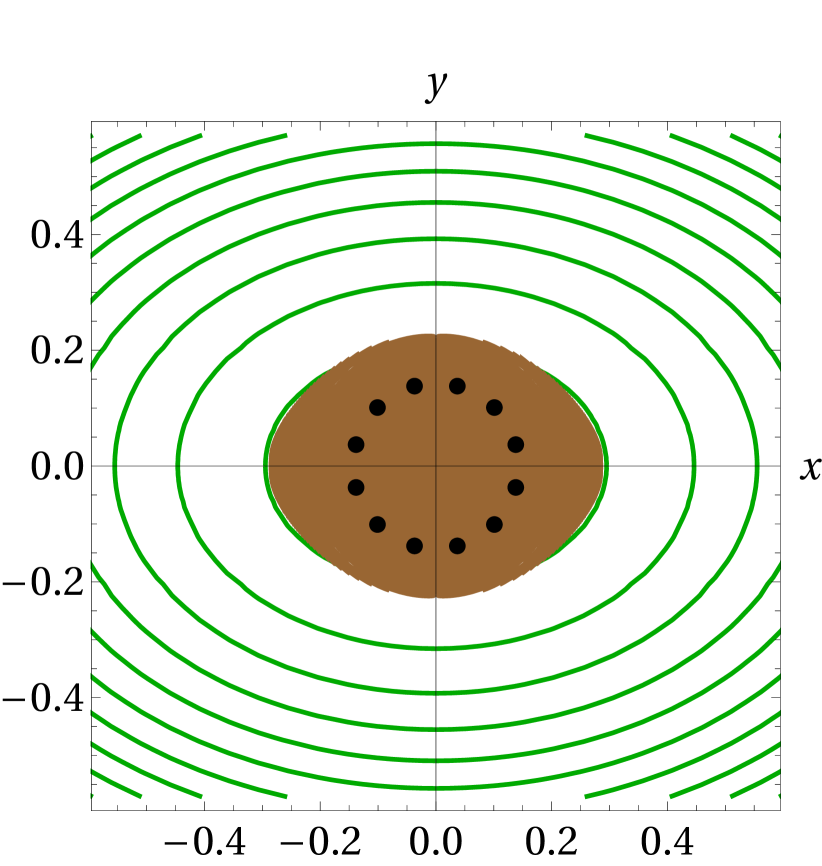
(b) For $\beta_{\bf e}=0.5$.

Figure 8: Numerically computed infrared optimal cosmological orbits of the canonical model (shown in brown) and level sets of ${\hat{\Phi}}$ (shown in green) near a critical cusp end ${\bf e}$, drawn in principal canonical coordinates centered at ${\bf e}$ for two values of $\beta_{\bf e}$. We took ${\bar{\lambda}}_{2}({\bf e})=1$, ${\hat{\bar{V}}}({\bf e})=1$ and $M_{0}=1$. The initial point $\varphi(0)$ of each orbit is shown as a black dot.

2.7 The IR behavior near an interior critical point

Let ${\bf c}$ be an interior critical point and $(x,y)$ be principal Cartesian canonical coordinates centered at ${\bf c}$. We have the metric:

$$\mathrm{d}s^{2}_{G}=\frac{4}{(1-\omega^{2})^{2}}[\mathrm{d}\omega^{2}+\omega^{2}\mathrm{d}\theta^{2}]~{}~{}$$

and:

$$V(\omega,\theta)=V({\bf c})+\frac{1}{2}\omega^{2}\left[\lambda_{1}({\bf c})\cos^{2}\theta+\lambda_{2}({\bf c})\sin^{2}\theta\right]+\mathrm{O}(\omega^{3})~{}~{},$$

where $\omega\stackrel{{\scriptstyle{\rm def.}}}{{=}}\sqrt{x^{2}+y^{2}}$ and $\theta\stackrel{{\scriptstyle{\rm def.}}}{{=}}\arg(x+\mathbf{i}y)$. Thus:

$$(\mathrm{grad}V)^{\omega}\!\approx\!\frac{(1-\omega^{2})^{2}}{4}\partial_{\omega}V\!=\!\frac{(1-\omega^{2})^{2}\omega}{4}[\lambda_{1}({\bf c})\cos^{2}\theta+\lambda_{2}({\bf c})\sin^{2}\theta]~{},$$

$$(\mathrm{grad}V)^{\theta}\!\approx\!\frac{(1-\omega^{2})^{2}}{4\omega^{2}}\partial_{\theta}V\!=\!\frac{(1-\omega^{2})^{2}}{4}[\lambda_{2}({\bf c})\!-\!\lambda_{1}({\bf c})]\sin(\theta)\cos(\theta)~{}.$$ (10)

The critical modulus $\beta_{\bf c}$ and characteristic signs $\epsilon_{1}({\bf c})$ and $\epsilon_{2}({\bf c})$ of $(\Sigma,G,V)$ at ${\bf c}$ are defined through:

$$\beta_{\bf c}\stackrel{{\scriptstyle{\rm def.}}}{{=}}\frac{\lambda_{1}({\bf c})}{\lambda_{2}({\bf c})}\in[-1,1]\setminus\{0\}~{}~{},~{}~{}\epsilon_{i}({\bf c})\stackrel{{\scriptstyle{\rm def.}}}{{=}}\mathrm{sign}(\lambda_{i}({\bf c}))~{}~{}(i=1,2)~{}~{}.$$

Distinguish the cases:

1. $\lambda_{1}({\bf c})=\lambda_{2}({\bf c}):=\lambda({\bf c})$, i.e. $\beta_{\bf c}=1$. Then $\epsilon_{1}({\bf c})=\epsilon_{2}({\bf c}):=\epsilon({\bf c})$ and ${\bf c}$ is a local minimum of $V$ when $\lambda({\bf c})$ is positive (i.e. when $\epsilon({\bf c})=1$) and a local maximum of $V$ when $\lambda({\bf c})$ is negative (i.e. when $\epsilon({\bf c})=-1$). Relations (2.7) become:

   $$(\mathrm{grad}V)^{\omega}\approx\frac{(1-\omega^{2})^{2}\omega}{4}\lambda({\bf c})~{}~{},~{}~{}(\mathrm{grad}V)^{\theta}\approx 0$$

   and the gradient flow equation of $(\Sigma,G,V)$ takes the following approximate form near ${\bf c}$:

   $$\frac{\mathrm{d}\omega}{\mathrm{d}q}=-\frac{(1-\omega^{2})^{2}\omega}{4}\lambda({\bf c})~{}~{},~{}~{}\frac{\mathrm{d}\theta}{\mathrm{d}q}=0~{}~{}.$$

   This gives $\theta=\mathrm{const}$, i.e. the gradient flow curves near ${\bf c}$ are approximated by straight lines through the origin when drawn in principal Cartesian canonical coordinates $(x,y)$ at ${\bf c}$;

2. $\lambda_{1}({\bf c})\neq\lambda_{2}({\bf c})$, i.e. $\beta_{\bf c}\neq 1$. When $\theta\in\{0,\frac{\pi}{2},\pi,\frac{3\pi}{2}\}$, the gradient flow equation reduces to:

   $$\frac{\mathrm{d}\omega}{\mathrm{d}q}=\frac{(1-\omega^{2})^{2}\omega}{4}\times\left\{\begin{array}[]{ll}\lambda_{1}({\bf c})&\mbox{if }\theta\in\{0,\pi\}\\ \lambda_{2}({\bf c})&\mbox{if }\theta\in\{\frac{\pi}{2},\frac{3\pi}{2}\}\end{array}\right.$$

   $$\frac{\mathrm{d}\theta}{\mathrm{d}q}=0~{}~{}.$$

   This gives four gradient flow orbits which are approximated near ${\bf c}$ by the principal geodesic orbits. When $\theta\not\in\{0,\frac{\pi}{2},\pi,\frac{3\pi}{2}\}$, the gradient flow equation takes the form:

   $$(1-\beta_{\bf c})\frac{\mathrm{d}\omega}{\mathrm{d}\theta}=\omega(\beta_{\bf c}\cot\theta+\tan\theta)~{}~{},$$ (12)

   with general solution:

   $$\omega=C\frac{|\sin(\theta)|^{\frac{\beta_{\bf c}}{1-\beta_{\bf c}}}}{|\cos(\theta)|^{\frac{1}{1-\beta_{\bf c}}}}~{}~{},~{}~{}\theta\not\in\{0,\frac{\pi}{2},\pi,\frac{3\pi}{2}\}~{}~{},~{}~{}C>0~{}.$$ (13)

Below we compare graphically the effective gradient flow orbits given by solutions of equation (13), depicted in Figure 9, to the numerically computed orbits of IR optimal cosmological curves, represented in Figure 10.

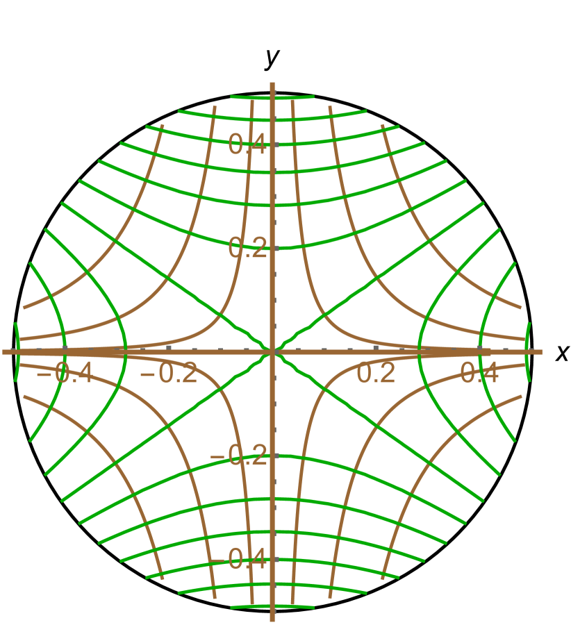
(a) $\beta_{\bf c}\!=\!-0.5$. Interior saddle point of $V$.

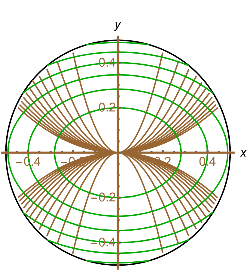
(b) $\beta_{\bf c}\!\!=\!0.5$. Local extremum of $V$.

Figure 9: Unoriented gradient flow orbits of $V$ (shown in brown) near an interior critical point superposed over the level lines of $V$ (shown in green) for two values of $\beta_{\bf c}$, plotted in principal Cartesian canonical coordinates centered at the critical point. The figure assumes $\omega_{\mathrm{max}}({\bf c})=0.5$. The principal coordinate axes correspond to the principal geodesic orbits at ${\bf c}$, which coincide with four special gradient flow orbits.

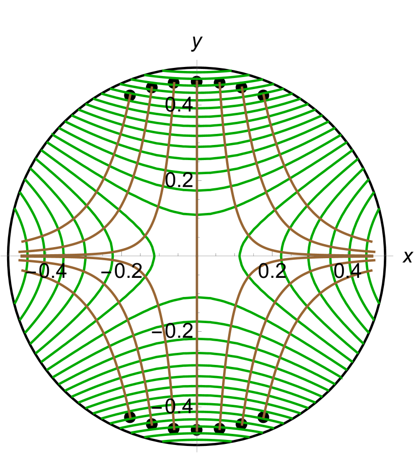
(a) Saddle point of $V$ for $\beta_{\bf c}\!=\!-0.5$. The dots are initial points $\varphi(0)$.

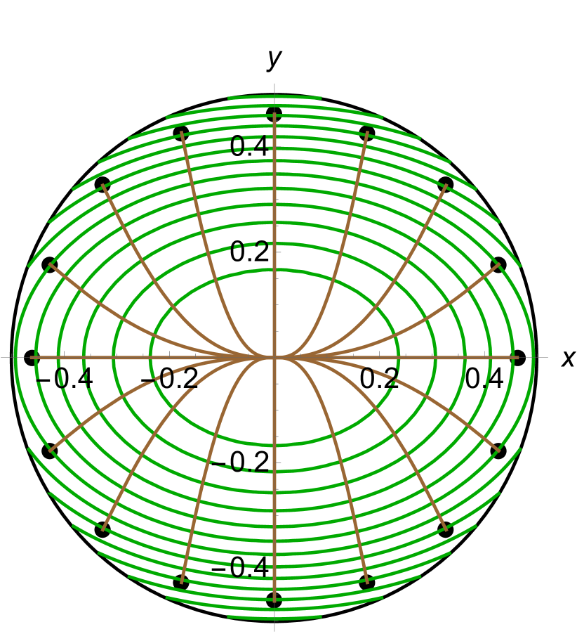
(b) Local extremum of $V$ for $\beta_{\bf c}\!\!=\!0.5$. The dots are initial points $\varphi(0)$.

Figure 10: Numerically computed orbits of infrared optimal cosmological curves $\varphi$ of the uniformized model (shown in brown) near an interior critical point ${\bf c}$, superposed over the level lines of $\Phi$ (shown in green) for two values of $\beta_{\bf c}$. Here $x,y$ are principal Cartesian canonical coordinates centered at the critical point. We assume $\omega_{\mathrm{max}}({\bf c})=0.5$. The initial points $\varphi(0)$ of these curves are shown as black dots.

3 Brief announcement of further results

Cosmological curves of two-field models can be approximated by mean field curves, using an approximation technique which is similar to the mean field approximation of condensed matter physics. Cosmological mean field approximations admits an elegant formulation using Ehresmann connections defined on the total space of the tangent bundle $T\Sigma$, i.e. rank two distributions $\mathcal{H}\subset TT\Sigma$ which are complementary to the vertical distribution $\mathcal{V}\subset TT\Sigma$ of the fiber bundle $T\Sigma\rightarrow\Sigma$. The corresponding mean field approximation replaces cosmological flow curves $\gamma=\dot{\varphi}:I\rightarrow T\Sigma$ of the model with the horizontal lift relative to $\mathcal{H}$ of curves in $\Sigma$ which satisfy the so-called mean field curve equation defined by $\mathcal{H}$. This amounts to treating as small the components of $\ddot{\varphi}:I\rightarrow TT\mathcal{M}$ which are “orthogonal” to $\mathcal{H}$ – in a sense which can be made precise.

The simplest approximations of this type are induced by the choice of a special coordinate system on an open subset of the tangent bundle $T\Sigma$, i.e. a coordinate system which naturally combines a coordinate system on the base $\Sigma$ with a coordinate system for the fibers of $T\Sigma$. In this case, the corresponding Ehresmann connection is flat and the mean field approximation amounts to neglecting the first time derivative of the two fiberwise coordinates, which are thereby being treated as “slow”. This parallels the logic of Born-Oppenheimer type approximations in quantum mechanics and statistical physics, which separate dynamical variables into “slow” and “fast” and treat the dynamics of slow variables approximately.

In our situation, the first order system of four ODEs which describes the cosmological equation in a given special coordinate system is replaced by the algebro-differential system in which the time derivatives of the fiberwise coordinates are set to zero. This leads to algebraic consistency conditions for the special coordinates called mean field equations, which determine a mean field surface inside $T\Sigma$; in many cases, the latter is a semialgebraic multisection of $T\Sigma$ defined on an open subset of the base $\Sigma$.

Mean field approximations of this type provide a very general procedure for extracting approximants of cosmological curves in various regimes, where the regime of interest is defined by the choice of fiberwise coordinates that one wishes to treat as “slow”. Since fiberwise coordinates are pairs of basic observables of the cosmological system which are functionally independent on an open subset of $T\Sigma$, each such regime is determined by the choice of a pair of locally independent on-shell cosmological observables. As we show in forthcoming work, a careful study of natural on-shell observables of two-field cosmological models provides interesting candidates for such fiberwise coordinates on $T\Sigma$, thus leading to natural mean field approximation schemes which have direct physics significance. The latter can be applied to any two-field model and in particular to tame hyperbolizable models.

One such mean field approximation is the so-called adapted approximation. This uses the fiberwise coordinates on $T\Sigma$ which are given by the projections of $\dot{\varphi}$ on the direction of the vector $\mathrm{grad}_{G}\Phi$ and on its positive normal direction and provides a mathematical refinement of the proposal of [24]. One can also consider the roll-turn approximation, which takes as fiberwise coordinates the on-shell second slow roll parameter and turning rate. Finally, one can consider the slow roll rate approximation, which uses the first and second on shell slow roll parameters as fiberwise coordinates.

Another kind of approximation which can be considered for two-field cosmological models is the so-called angular approximation, which arises by neglecting the first two time derivatives of the radial variable in a given semigeodesic coordinate system $(r,\theta)$. This provides approximants on each semigeodesic coordinate patch, whose accuracy can be characterized theoretically and computed numerically.

In forthcoming work, we study the approximations mentioned above for tame two-field cosmological models and the corresponding error terms, which play an important role when ascertaining their accuracy (see [8]). In particular, this serves as a test of various proposals made previously in the literature. Moreover, we compare these approximations with the IR approximation studied in [22] (and summarized above) near interior critical points and near ends of $\Sigma$, determining the regimes within which the various approximations are accurate.

4 Conclusions

We studied the first order IR behavior of tame hyperbolizable two-field cosmological models by analyzing the asymptotic form of the gradient flow orbits of the classical effective scalar potential $V$ with respect to the uniformizing metric $G$ near all interior critical points and ends of $\Sigma$. We showed that the IR behavior of tame hyperbolizable two-field cosmological models is characterized by a finite set of parameters associated to their ends and interior critical points. Comparing with numerical computations, we found that the first order IR approximation is already quite good for all interior critical points and all ends except for cusps, for which one must consider higher order corrections in the IR expansion in order to obtain a good approximation. Our results characterize the IR universality classes of all tame hyperbolizable two-field models in terms of geometric data extracted from the asymptotic behavior of the effective scalar potential and uniformizing metric.

Since the Morse assumption on the extended potential determines its asymptotic form near all points of interest on $\widehat{\Sigma}$, we could derive closed form expressions for the asymptotic gradient flow which describes the corresponding infrared phases of such models in the sense of [9]. In particular, we found that the asymptotic gradient flow of $(\Sigma,G,V)$ near each end which is a critical point of the extended potential can be expressed using the incomplete gamma function of order two and certain constants which depend on the type of end under consideration and on the principal values of the extended effective potential $\widehat{V}$ at that end. We also found that flaring ends which are not critical points of $\widehat{V}$ act like fictitious but non-standard stationary points of the effective gradient flow. While the local form near the critical points of $V$ is standard (since they are hyperbolic stationary points [25, 26] of the cosmological and gradient flow), the asymptotic behavior near Freudenthal ends is exotic in that some of the ends act like fictitious stationary points with unusual characteristics.

We compared these results with numerical computations of cosmological curves near the points of interest. We found particularly interesting behavior near cusp ends, around which generic cosmological trajectories tend to spiral a large number of times before either “falling into the cusp” or being “repelled” back toward the compact core of $\Sigma$ along principal geodesic orbits determined by the classical effective potential $V$. In particular, cusp ends lead naturally to “fast turn” behavior of cosmological curves.

References

- [1] C. Vafa, The string landscape and the swampland, [hep-th/0509212].
- [2] H. Ooguri, C. Vafa, On the geometry of the string landscape and the swampland, Nucl. Phys. B 766 (2007) 21-33 [hep-th/0605264].
- [3] T. D. Brennan, F. Carta, C. Vafa, The String Landscape, the Swampland, and the Missing Corner, TASI2017 (2017) 015 [hep-th/1711.00864].
- [4] M. van Beest, J. Calderon-Infante, D. Mirfendereski, I. Valenzuela, Lectures on the Swampland Program in String Compactifications, [hep-th/2102.01111].
- [5] A. Achucarro, G. A. Palma, The string swampland constraints require multi-field inflation, JCAP 02 (2019) 041 [hep-th/1807.04390].
- [6] G. Obied, H. Ooguri, L. Spodyneiko, C. Vafa, De Sitter Space and the Swampland, [hep-th/1806.08362].
- [7] S.K. Garg, C. Krishnan, Bounds on Slow Roll and the de Sitter Swampland, JHEP 11 (2019) 075 [hep-th/1807.05193].
- [8] L. Anguelova, C.I. Lazaroiu, Dynamical consistency conditions for rapid turn inflation, JCAP 05 (2023) 020 [hep-th/2210.00031].
- [9] C. I. Lazaroiu, Dynamical renormalization and universality in classical multifield cosmological models, Nucl. Phys. B 983 (2022), 115940 [hep-th/2202.13466].
- [10] C. I. Lazaroiu, C. S. Shahbazi, Generalized two-field -attractor models from geometrically finite hyperbolic surfaces, Nucl. Phys. B 936 (2018) 542-596.
- [11] E. M. Babalic, C. I. Lazaroiu, Generalized -attractor models from elementary hyperbolic surfaces, Adv. Math. Phys. 2018 (2018) 7323090 [hep-th/1703.01650].
- [12] E. M. Babalic, C. I. Lazaroiu, Generalized -attractors from the hyperbolic triply-punctured sphere, Nucl. Phys. B 937 (2018) 434-477 [hep-th/1703.06033].
- [13] L. Anguelova, E. M. Babalic, C. I. Lazaroiu, Two-field Cosmological -attractors with Noether Symmetry, JHEP 04 (2019) 148 [hep-th/1809.10563].
- [14] L. Anguelova, E. M. Babalic, C. I. Lazaroiu, Hidden symmetries of two-field cosmological models, JHEP 09 (2019) 007 [hep-th/1905.01611].
- [15] L. Anguelova, On Primordial Black Holes from Rapid Turns in Two-field Models, JCAP 06 (2021) 004 [hep-th/2012.03705].
- [16] L. Anguelova, J. Dumancic, R. Gass, L. C. R. Wijewardhana, Dark Energy from Inspiraling in Field Space, [hep-th/2111.12136].
- [17] C. I. Lazaroiu, Hesse manifolds and Hessian symmetries of multifield cosmological models, Rev. Roum. Math. Pures Appl. 66 (2021) 2, 329-345 [hep-th/2009.05117].
- [18] E. M. Babalic, C. I. Lazaroiu, Two-field cosmological models and the uniformization theorem, Springer Proc. Math. Stat., Quantum Theory and Symmetries with Lie Theory and Its Applications in Physics 2 (2018) 233-241 [hep-th/1801.03356].
- [19] E. M. Babalic, C. I. Lazaroiu, Cosmological flows on hyperbolic surfaces, Facta Universitatis, Ser. Phys. Chem. Tech. 17 (2019) 1, 1-9 [hep-th/1810.00441].
- [20] L. Anguelova, E. M. Babalic, C. I. Lazaroiu, Noether Symmetries of Two-Field Cosmological Models, AIP Conf. Proc. 2218 (2020) 050005 [hep-th/1910.08441].
- [21] L. Anguelova, Primordial Black Hole Generation in a Two-field Inflationary Model, In: Dobrev, V. (eds) Lie Theory and Its Applications in Physics. LT 2021. Springer Proc Math. Stat. 396. Springer, Singapore [hep-th/2112.07614.]
- [22] E. M. Babalic, C. I. Lazaroiu, The infrared behavior of tame two-field cosmological models, Nucl. Phys. B 983 (2022), 115929 [hep-th/2203.02297].
- [23] H. Freudenthal, Über die Enden topologischer Räume und Gruppen, Math. Z. 33 (1931) 692-713.
- [24] T. Bjorkmo, Rapid-Turn Inflationary Attractors, Phys. Rev. Lett. 122 (2019) 251301, [hep-th/1902.10529].
- [25] J. Palis Jr., W. De Melo, Geometric theory of dynamical systems: an introduction, Springer, New York, U.S.A. (2012).
- [26] A. Katok, B. Hasselblatt, Introduction to the modern theory of dynamical systems, Cambridge U.P., 1995.