Exploring Singularities in point clouds with the graph Laplacian: An explicit approach

Abstract.

We develop theory and methods that use the graph Laplacian to analyze the geometry of the underlying manifold of point clouds. Our theory provides theoretical guarantees and explicit bounds on the functional form of the graph Laplacian, in the case when it acts on functions defined close to singularities of the underlying manifold. We also propose methods that can be used to estimate these geometric properties of the point cloud, which are based on the theoretical guarantees.

1. Introduction

High dimensional data is common in many research problems across academic fields. It is often assumed that a data set $X=\{X_{i}\}_{i}^{n}\subset\mathbb{R}^{N}$ lies on a lower-dimensional set $\Omega$ and is in fact a sample from a probability distribution over $\Omega$. It is also often assumed that $\Omega$ can be represented as the union of several manifolds $\Omega_{i}$, where each $\Omega_{i}$ represents a different class in a classification problem. For instance, if a data set contains two classes, $i$ and $j$, class $i$ might be contained in $\Omega_{i}$ and class $j$ in $\Omega_{j}$, with the two classes potentially being disjoint. However, classification is not always so clear-cut: For instance, in the MNIST dataset, where handwritten digits of $"1"\in\Omega_{1}$ and $"7"\in\Omega_{7}$ can appear very similar, suggesting that $\Omega_{1}\cap\Omega_{7}\neq\emptyset$. Therefore, understanding geometric situations such as intersections is of interest in classification problems.

In the manifold model of data, an intersection between two different manifolds $\Omega_{i},\Omega_{j}$ is either represented just as such, or it can be viewed as a singularity if we consider $\Omega=\Omega_{i}\cup\Omega_{j}$ as a single manifold. Other regions in $\Omega$ that can be viewed as singular, such as boundaries and edges, may also be of interest as they can signify important features in the data.

To study such singularities, we use the graph Laplacian $L_{n,t}$. This operator, which depends on the number of data points $n$ and a parameter $t$, can act on functions defined on the data set $X$. As $n$ tends to infinity and $t$ tends to 0, $L_{n,t}$ converges to the Laplace-Beltrami operator in the interior of a single manifold [1]. In this work, we primarily study the behavior of $x\to L_{n,t}f(x)$ for functions $f$, when $x$ is close to singular points.

Our contribution in this paper is primarily an extension and reframing of work done in [2]. At the same time, we also focus on the specific case when the function $f$ is assumed to be of the form $f(x)=v\cdot x$, where $v$ is a unit vector. We also consider more restricted classes of manifolds.

Since $L_{n,t}$ converges to Laplace-Beltrami, a second order differential operator, in the interior of $\Omega$, we expect that for $f$ as above $L_{n,t}f(x)\approx 0$. However, for singular points like intersections, the limit operator is of first order [2], and $L_{n,t}f(x)\neq 0$, which can be seen in Fig. 1.

Our results show how $x\to L_{t}f(x)$ and, through a finite-sample bound, how $x\to L_{n,t}f(x)$ behaves. More specifically, given $x_{0}\in\Omega_{i}$ near some singularity, and $x$ in the ball $B_{R}(x_{0})$, including the case when $x\not\in\Omega_{i}$, we show how the function $x\to L_{n,t}f(x)$ deviates from being constantly 0 and has specific functional forms. These forms depend on the type of singularity. In [2] they showed what these forms are, up to some asymptotically defined error term, as $t\to 0$, We build on this to get explicit expressions of $L_{t}f(x)$ when $t$ is fixed.

Overview of results: First, in Section 4.1 we consider the case that $\Omega$ is flat manifold of dimension $d$, and where we have a geometric situation similar to Fig. 3.

To set up the results, we start with an $x_{0}\in\Omega$, and let $x\in B_{R}(x_{0})$, where $R=\sqrt{t}r_{0}>0$, and use $\hat{x}$ to denote the projection of $x$ to $\Omega$. We also define $v_{n,\Omega}$ as the projection of $v$ onto $x-\hat{x}$, and $v_{n,\partial\Omega}$ is the projection of $v$ onto the outwards normal of $\partial\Omega$. Then we show the following:

• In Theorem 1, we let $\|x-x_{0}\|=r\sqrt{t}$ and $\theta$ is the angle between vectors $x-x_{0}$ and $\hat{x}-x_{0}$. If $x$ is not close to $\partial\Omega$, then

  $$L_{t}f(x)=A(x)t^{\frac{d+1}{2}}v_{n,\Omega}\sin(\theta)re^{-\sin^{2}(\theta)r^{2}}+t^{\frac{d+1}{2}}B(x).$$

  The function $A$ is close to being constantly equal to $\pi^{d/2}$, and $B$ can be made, uniformly, arbitrarily small. Both functions have explicit bounds.

• Theorem 2 shows what happens when $x$ is close to $\partial\Omega$:

  $$L_{t}f(x) =\widehat{A}_{1}(x)t^{\frac{d+1}{2}}v_{n,\Omega}\sin(\theta)re^{-\sin^{2}(\theta)r^{2}}$$

  $$\qquad+\widehat{A}_{2}(x)t^{\frac{d}{2}}v_{n,\partial\Omega}e^{-\sin^{2}(\theta)r^{2}}\quad+B(x)t^{\frac{d+1}{2}}e^{-r_{0}^{2}},$$

  where functions $\widehat{A}_{1},\widehat{A}_{2}$ and $B$ have explicitly computable bounds.

In Section 4.2 and Section 4.3 we prove more general results:

• In Theorem 3 we relax the conditions on $\Omega$, considering non-flat manifolds, and prove a weaker version of Theorem 1.

• In Theorem 4 we relax the conditions further, and allow for noise when sampling from $\Omega$.

To connect $L_{t}$ to $L_{n,t}$, in Section 4.4 we prove two finite-sample bounds.

Finally, in Section 5.1 we propose methods to find intersections in data and estimate the angle of such intersections, which are motivated by the aforementioned theorems and Corollary 4.5. We also provide numerical experiments, in Section 5, to test these methods.

2. Earlier work

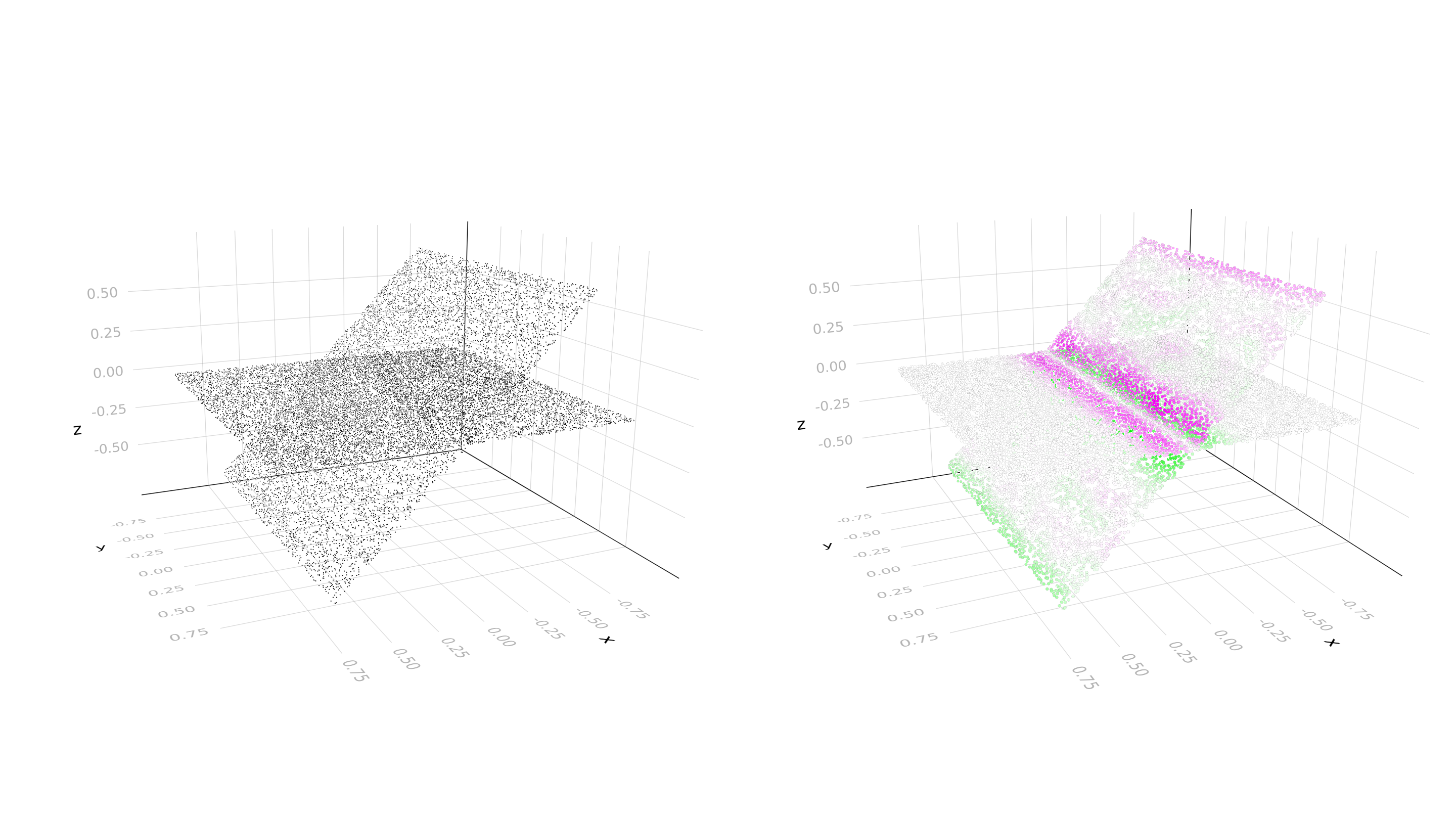
Figure 1. Graph Laplacian $L_{n,t}$ acting on a linear function $f$. Purple color showing positive, and green color negative values of $L_{n,t}f$, where lack of color indicates values near 0

The framework of assuming an underlying low-dimensional manifold of data, in conjunction with graph-related tools and in particular the graph Laplacian, has been used extensively. Some examples include work in clustering [3, 4, 5, 6, 7], dimensionality reduction [8, 9], and semi-supervised learning [10].

Several of the approaches to study data sets that use the graph Laplacian leverage that if the manifold is smooth enough and well-behaved, then the graph Laplacian approximates some well-understood operator (for instance the Laplace-Beltrami operator [11]), which has useful mathematical properties.

Therefore, the question of convergence properties of the graph Laplacian is useful and important, and it has partly been explicated in [1, 12, 13, 9]. In particular, and highly influential of this paper, is what the asymptotic convergence looks like near singularities of the manifold, which was shown in [2].

3. Basic mathematical objects and theory

In this section, we provide more precise definitions and introduce the basic mathematical theory we will be using to present and prove our results. This is similar to the problem setup in [2].

3.1. Conditions on manifolds

We will consider sets of the form $\Omega=\cup_{i}^{m}\Omega_{i}$, where each $\Omega_{i}$ is a smooth and compact $d$-dimensional Riemannian submanifold of $\mathbb{R}^{N}$. We will assume that if $\Omega_{i},\Omega_{j}$, and $i\neq j$ have a non-empty intersection, then this intersection will have dimension lower than $d$.

Associated to $\Omega$ will be a probability measure with density $p:\Omega\to\mathbb{R}$ such that the restriction of $p$ to $\Omega_{i}$ is smooth, and there are constants $a$ and $b$ such that $0<a\leq p\leq b$.

If $x\in\Omega_{i}$, we can consider the tangent space $T_{\Omega_{i},x}\simeq\mathbb{R}^{d}$, which we will identify as a subspace of the ambient space $\mathbb{R}^{N}$. More precisely, given open subsets $U\subset\mathbb{R}^{d}$ and $W\subset\Omega_{i}$ ($W$ is open in the subspace topology of $\Omega_{i}$), and a coordinate chart $\alpha:U\to W$ such that $\alpha(0)=x$, we define $T_{\Omega_{i},x}$ as the image of $\mathbb{R}^{d}$ under the action of the Jacobian. We denote the Jacobian $D\alpha:U\to\mathbb{R}^{N\times d}$, evaluated at 0, by $D\alpha(0)$. The best linear approximation to $u\mapsto\alpha(u)$ is of course given by $u\mapsto x+D\alpha(0)u$, and $x+T_{\Omega_{i},x}$ is the best flat approximation to $\Omega_{i}$ around $x$.

The definition of $\Omega$ implies that a point $x\in\Omega$ can have more than one associated tangent space. For example, if $x\in\Omega_{i}\cap\Omega_{j}$ and $i\neq j$, then both $T_{\Omega_{i},x}$ and $T_{\Omega_{j},x}$ exist, and they can be different.

A note on notation is that we will denote the interior of a manifold $\Omega_{i}$ by $\operatorname{Int}\Omega_{i}$, and the boundary by $\partial\Omega_{i}$.

3.2. Types of singularities

The following are what we will refer to as singular points, which will be of four different kinds. Given $x\in\Omega=\cup\Omega_{i}$, we have the following types:

1. There is a submanifold $\Omega_{i}$ such that $x\in\partial\Omega_{i}$.

2. There are submanifolds $\Omega_{i}\neq\Omega_{j}$ such that $x\in\operatorname{Int}\Omega_{i}\cap\operatorname{Int}\Omega_{j}$.

3. There are submanifolds $\Omega_{i}\neq\Omega_{j}$ such that $x\in\partial\Omega_{i}\cap\operatorname{Int}\Omega_{j}$.

4. There are submanifolds $\Omega_{i}\neq\Omega_{j}$ such that $x\in\partial\Omega_{i}\cap\partial\Omega_{j}$.

The different types above can of course have non-empty intersection with each other, and a non-singular point is simply a point $x\in\operatorname{Int}\Omega_{i}$ such that if $j\neq i$, then $x\neq\Omega_{j}$. See Fig. 2 for two examples of singularities.

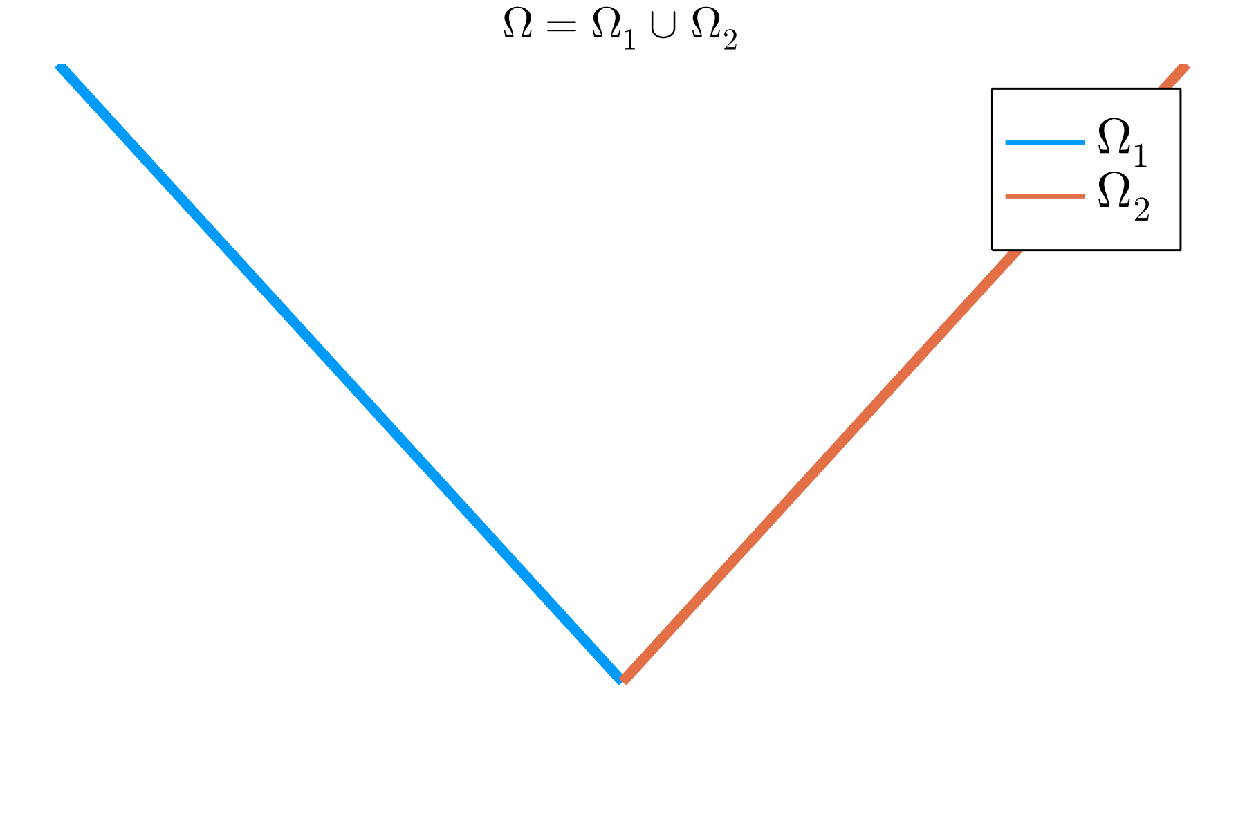
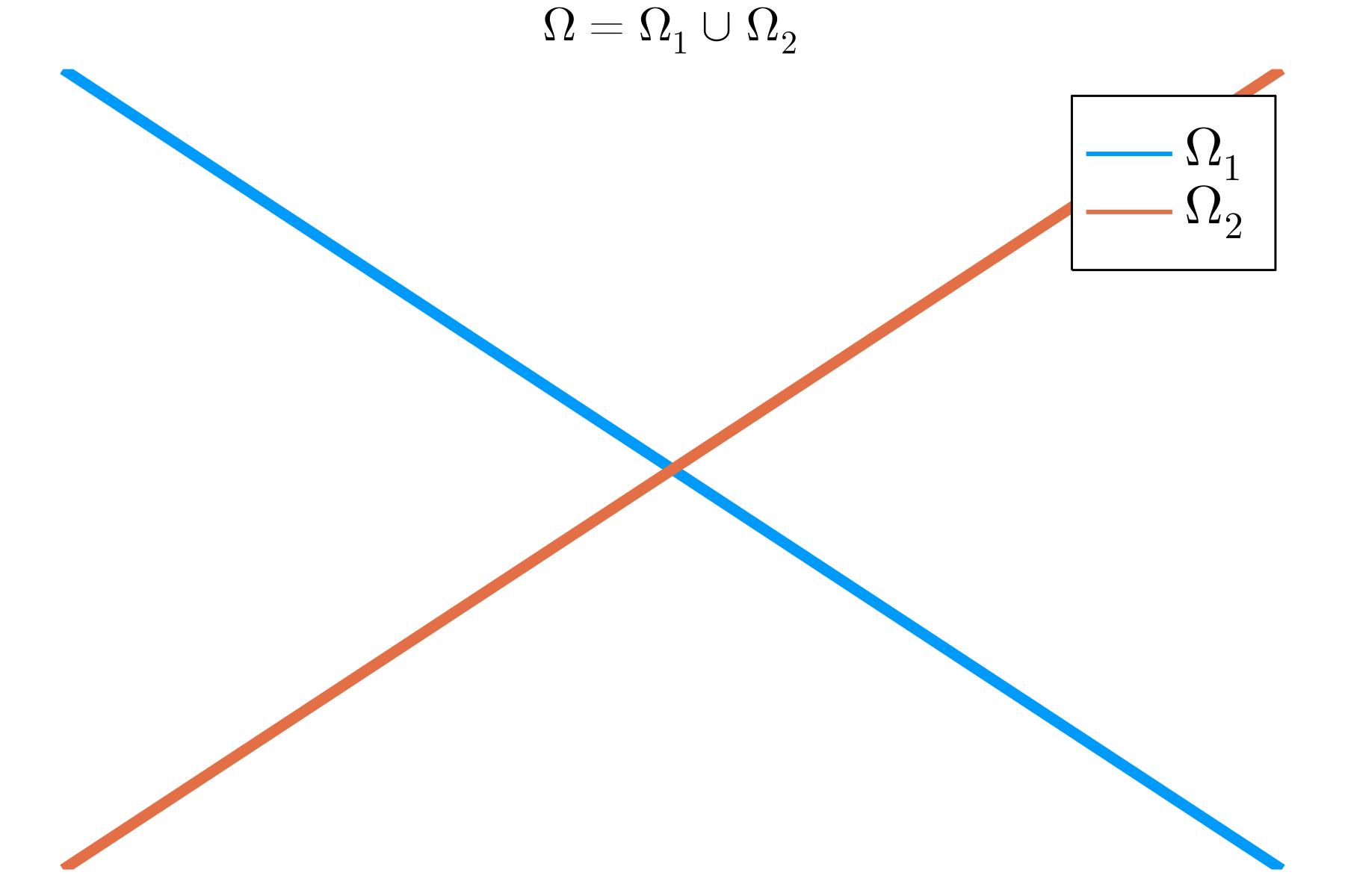
Figure 2. There is a singularity in the intersection of the lines above. The left figure shows a point of Type 4, and the right figure shows a point of Type 2.

3.3. Integration on $\Omega$

We will integrate scalar-valued functions, $f:\Omega\to\mathbb{R}$, over $\Omega$. When formulating integration of scalar-valued functions over submanifolds of $\mathbb{R}^{N}$, we follow the approach in [14]. Because we need some preliminary results concerning integration on $\Omega$, we make some important definitions explicit.

First, let $x_{1},\ldots,x_{k}$ be vectors in $\mathbb{R}^{N}$ for $k\leq N$. If $I=(i_{1},i_{2},\dots,i_{k})$ is a $k$-tuple of integers such that $i_{1}\leq i_{2}\leq\cdots\leq i_{k}$, define $X_{I}\in\mathbb{R}^{k\times k}$ as the $k\times k$ matrix containing only rows $i_{1},\dots,i_{k}$ of the matrix $X=(x_{1},\ldots,x_{k})$. Now we can define the volume function $V:R^{N\times k}\to\mathbb{R}$, by $V(X)=\sqrt{\det^{2}(X^{t}X)}=\left[\sum_{I}\det^{2}X_{I}\right]^{1/2}$, where the $I$’s span over $k$-tuples as above, see [14, Theorem 21.4].

In general, given a coordinate chart $\alpha:U\to W$, where $U\subset\mathbb{R}^{d}$, $W\subset\Omega_{i}\subset\mathbb{R}^{N}$ are open subsets, and $D\alpha$ is the Jacobian of $\alpha$, we can express integration over $W$ as

$$\int_{W}f\,{\rm d}V=\int_{U}f\circ\alpha\,\mathrm{V}(D\alpha).$$

In the coming proofs, when integrating around a point $x\in\operatorname{Int}\Omega_{i}$, we will change coordinates to the standard basis in $T_{\Omega_{i},x}=\mathbb{R}^{k}$. With this we mean that we can find open sets $W\subset\Omega_{i}$ around $x$ such that the projection map $\pi:W\to B\subset x+T_{\Omega_{i},x}$ is a diffeomorphism, where $x+T_{\Omega_{i},x}\coloneqq\{\,x+y\mid y\in T_{\Omega_{i},x}\,\}$. To integrate over $T_{\Omega_{i},x}$ we use the map $\pi^{-1}$ precomposed with an inclusion map.

More specifically and without loss of generality, by translation and an orthonormal coordinate change, we can assume that $T_{\Omega_{i},x}=\mathbb{R}^{d}\times\{0\}^{n-d}$. In this coordinate system we can write

$$\alpha:U\xrightarrow{i}x+T_{\Omega_{i},x}\xrightarrow{\pi^{-1}}W\subset\Omega_{i},$$ (3.1)

where $i$ is the natural inclusion map and $U$ an open subset in $\mathbb{R}^{k}$.

3.4. Important bounds

The following bounds will be used later in our proofs: First, let $T_{\Omega,x},U,W,\pi$ be as in Section 3.3. Then for any $y\in W$,

$$\left\lVert y-\pi(y)\right\rVert\leq O(\left\lVert x-\pi(y)\right\rVert^{2}).$$ (3.2)

This follows since $\Omega_{i}$ is smooth and the tangent space represents the best flat approximation of $\Omega_{i}$ around $x$.

To formulate the second bound, we need the lemma below.

Lemma 3.1.

Let $U,W,x,y,\Omega_{i},\pi,i,\alpha$ be as in Section 3.3. Then the following holds for the volume function $V$:

$$V(D\alpha(y))=1+O(\left\lVert x-\pi(y)\right\rVert^{2}).$$

Proof.

Since $\alpha=\pi^{-1}\circ i$, and the tangent space is the best flat approximation of $\Omega$, we can parametrize the $W$ by $\alpha(u)=(u,g(u))$. It is then easy to see that for $i=1,\ldots,d$ we have

$$\partial_{i}\alpha(y)=(e_{i},\partial_{i}g(u)),$$

where $\partial_{i}g(0)=0$ and $\left\lVert\partial_{i}g(u)\right\rVert=O(\left\lVert u\right\rVert)$. Now

$$\det D\alpha_{I}=\begin{cases}1&\text{if $I=(1,2\dots,d)$}\\ O(\left\lVert u\right\rVert)&\text{otherwise.}\end{cases}.$$

If we Taylor expand $x\to\sqrt{x}$, we get

$$V(D\alpha)=\left(\sum_{I}(\det D\alpha_{I})^{2}\right)^{1/2}=1+O(\left\lVert u\right\rVert^{2}),$$

and by applying the above on $(u,0)=x-\pi(y)$ we are finished. ∎

Further, since we have a finite union $\Omega=\cup_{i}\Omega_{i}$ and each $\Omega_{i}$ is compact, 3.2, the previous lemma implies that we can find a uniform bound $L$ such that for all tuples $(U,W,x,y,\pi,\Omega_{i})$

$$\left\lVert y-\pi(y)\right\rVert\leq L\left\lVert x-\pi(y)\right\rVert^{2}$$ (3.3)

and

$$|V(D\alpha)-1|\leq L\left\lVert x-\pi(y)\right\rVert^{2}$$ (3.4)

holds.

3.4.1. $(L,r)$-regular manifolds

To formulate our results we will need some measure of how regular, with regard to curvature, our set $\Omega$ is. The following definition captures the necessary information.

Definition 3.2.

Let $\Omega=\cup\Omega_{i}$ be a union of compact submanifolds in $\mathbb{R}^{N}$. We also let $r>0$ be the largest radius such that any point $x\in\operatorname{Int}\Omega$ allows coordinate charts $\alpha:U\to B_{r}(x)\cap\Omega_{i}$, where $U\subset\mathbb{R}^{d}$ and $B_{r}(x)\subset\mathbb{R}^{N}$ is an open ball of radius $r$ around $x$. Further, assume also that conditions (3.3) and (3.4) hold over all tuples $(U,W,x,y,\pi,\Omega_{i})$ for some $L>0$. Then we say that $\Omega$ is $(L,r)$-regular.

Example 3.3.

Any smooth and compact submanifold is $(L,r)$-regular. For instance the graph of the function $x\to x^{2}$ over the compact interval $[-1,1]$ is $(1,1)$-regular.

3.5. Graph Laplacian

In this section we introduce the graph Laplacian and how it acts on real-valued functions defined on $\mathbb{R}^{N}$.

Given $n$ i.i.d. random samples $X=\{X_{1},\ldots,X_{n}\}$ from the distribution with density $p$ on $\Omega$, we build a weighted fully connected graph $G=(V,E)$ as follows: We let each sample $X_{i}$ represent a vertex $i$, and for vertices $i,j\in V$ the weight on $(i,j)\in E$ is given by

$$W_{n,t}(i,j):=W_{n,t}(X_{i},X_{j})=\frac{1}{n}K_{t}(X_{i},X_{j})=\frac{1}{n}e^{-\frac{\|X_{i}-X_{j}\|^{2}}{t}}.$$

The function $W_{n,t}$ is naturally viewed as an $n\times n$ matrix, and the variable $t$ is in the literature often referred to as the bandwidth of the kernel $K_{t}$.

Remark 3.4.

In the limit analysis as $n\to\infty$, it is useful also normalize by $\frac{1}{t^{d/2+1/2}}$. But, since a priori we do not know the dimension $d$, we will work without this normalization.

We define the diagonal weighted degree matrix as

$$D_{n,t}(i,i)=\sum_{j}W_{n,t}(i,j),$$

and the graph Laplacian $L_{n,t}$ as

$$L_{n,t}=D_{n,t}-W_{n,t}.$$

Remark 3.5.

This is often referred to as the unnormalized graph Laplacian. There are other normalizations of this matrix which are used, for example, in [6, 7, 13]. One difference between these normalizations are their limit properties.

Given the fully connected graph $G=(E,V)$, the graph Laplacian above can be seen as an operator acting on arbitrary functions $f:V\to\mathbb{R}$ in the following way:

$$L_{n,t}f(X_{i})=\frac{1}{n}\sum_{j}K_{t}(X_{i},X_{j})(f(X_{i})-f(X_{j})),\quad(X_{i},X_{j})\in E.$$

We extend this operator to acting on functions $f\in C_{c}(\mathbb{R}^{N},\mathbb{R})$, by the canonical choice

$$L_{n,t}f(x)=\frac{1}{n}\sum_{j}K_{t}(x,X_{j})(f(x)-f(X_{j})),\quad x\in\mathbb{R}^{N}.$$ (3.5)

Our main results will be stated in terms of the expected operator:

$$L_{t}f(x)=\mathbb{E}_{p}[L_{n,t}f(x)]=\int_{\Omega}K_{t}(x,y)(f(x)-f(y))p(y)\,{\rm d}y.$$ (3.6)

That this is well-defined follows from the assumptions that $X_{1},\dots,X_{n}$ are i.i.d., that $f$ is continuous and that $\Omega$ is compact.

One immediate consequence of the linearity of the integral is that

$$\begin{split}L_{t}f(x)&=\int_{\Omega}K_{t}(x,y)(f(x)-f(y))\,{\rm d}y\\ &=\sum_{i}\int_{\Omega_{i}}K_{t}(x,y)(f(x)-f(y))p(y)\,{\rm d}y.\end{split}$$ (3.7)

In our approach it is useful to work with the restricted Laplacian $L_{t}^{i}$, which is defined by

$$L_{t}^{i}f(x)=\int_{\Omega_{i}}K_{t}(x,y)(f(x)-f(y))p(y)\,{\rm d}y.$$ (3.8)

3.6. Gamma functions

In the proofs of several of our results we will need to handle the Gamma function $\Gamma(\cdot)$, and both the lower and upper incomplete gamma functions, $\gamma(\cdot,\cdot)$ and $\Gamma(\cdot,\cdot)$ respectively. These are well-known and are defined by the equations

$$\Gamma(a) =\int_{0}^{\infty}t^{a-1}e^{-t}\,{\rm d}t,$$

$$\gamma(a,x) =\int_{0}^{x}t^{a-1}e^{-t}\,{\rm d}t,$$

$$\Gamma(a,x) =\int_{x}^{\infty}t^{a-1}e^{-t}\,{\rm d}t.$$

In this paper both $a$ and $x$ are non-negative real numbers.

We will need the following bounds: First, if $a\geq 1$, then $t^{a-1}\geq x^{a-1}$ and

$$\Gamma(a,x)\geq x^{a-1}\int_{x}^{\infty}e^{-x}\,{\rm d}t=x^{a-1}e^{-x}.$$ (3.9)

Secondly, if $e^{x}>2^{a}$, then by [15, Theorem 4.4.3],

$$\Gamma(a,x)\leq ax^{a-1}e^{-x}.$$ (3.10)

Finally, we need the lower bound

$$\gamma(a,a)\geq\frac{1}{2}\Gamma(a).$$ (3.11)

That this holds can be seen by viewing $\gamma(a,x)$ as an unnormalized version of the cumulative distribution function of the Gamma distribution, for which it is well-known that the median $\nu$ is less than $a$.

4. Main results

Now that we have the necessary definitions and mathematical background, we are ready to present and prove our main results. Before stating the theorems, we will provide a brief section that explains the geometry of some terms that will be used in the theorem statements. This will help make the theorems easier to understand.

Remark 4.1.

Some of our results are given in the particular case when $\Omega=\cup\Omega_{i}$ is such that each $\Omega_{i}$ is flat. This is easier to analyze and gives better bounds, but it is also motivated by a particular use-case: Sets of the form

$$\Omega_{:}=\{W\in\mathbb{R}^{k}:|f_{W}(x)-g(x)|=0,\quad x\in\mathcal{D}\},$$

where $f_{W}$ is a neural network with weights $W$ and ReLU activation functions. Here $g$ is a target function, and $\mathcal{D}$ some dataset. That is, the zero sets of the optimization problem which one tries to minimize during training of a common type of neural network.

General structure of results

By 3.7 it is enough to understand the restricted Laplacian, $L^{i}_{t}$ defined in 3.8. Because of this, our results are formulated to show the behavior of $L^{i}_{t}$. Depending on what type of singularity being examined, it is easy to extend the results to the full Laplacian. In Corollary 4.5 we give one example of how to extend the results to the sum $\sum_{i=1}^{2}L^{i}_{t}$ when one is close to an intersection of two manifolds.

Geometry and notation for Section 4.1

We will in several theorems also formulate the function $x\to L_{t}^{i}f(x)$ partly in terms of new coordinates $(r,\theta)$. Here $r$ is defined by the relation $\left\lVert x-x_{0}\right\rVert=\sqrt{t}r$, and given the projection $\hat{x}$ of $x$ to a plane $\Omega_{i}$, we define $\theta\in[0,\pi/2]$ to be the angle between vectors $x_{0}-x$ and $\hat{x}-x$, as the schematic in Fig. 3. By simple geometry, it also follows that $\left\lVert\hat{x}-x\right\rVert=r\sin\theta$.

Given a vector $v\in\mathbb{R}^{N}$, we will have reason to write the expression $v\cdot(\hat{x}-x)$ as

$$v\cdot(\hat{x}-x)=r\sqrt{t}\sin(\theta)v\cdot\frac{\hat{x}-x}{\left\lVert\hat{x}-x\right\rVert}=r\sqrt{t}\sin(\theta)v_{n,\Omega_{i}}(x),$$

where we have defined

$$v_{n,\Omega_{i}}(x)\coloneqq v\cdot\frac{\hat{x}-x}{\left\lVert\hat{x}-x\right\rVert}.$$

In other words, $v_{n,\Omega_{i}}$ is the projection of $v$ onto a unit normal vector of $\Omega_{i}$, but it depends on $x$. We define this function to be 0 when $x=\hat{x}$, and let us note that for $x\neq\hat{x}$, this function is constant up to its sign. This implies that evaluating $r\sqrt{t}\sin(\theta)v_{n,\Omega_{i}}(x)$ is the same as letting $v_{n,\Omega_{i}}$ be fixed, but allowing $\theta$ to change sign depending on which side of $\Omega_{i}$ $x$ is, i.e. as if we have fixed the coordinate system in which we measure the angle $\theta$. We will in our theorem statements suppress the $x$-dependancy of $v_{n,\Omega_{i}}$, to increase readability.

Additionally, in Theorem 2 we will have a term $v_{n,\partial\Omega_{i}}$ that is specific to that theorem. This will be defined in the case where there is a boundary close to $x$. In Fig. 3, this would imply there is a boundary of $\Omega_{1}$ nearby. To give the definition if this term, we first let $\hat{x}_{\partial\Omega_{i}}$ be the projection of $\hat{x}$ to $\partial\Omega_{i}$. We can now define a unit normal at $\hat{x}_{\partial\Omega_{i}}$, denoted by $n_{\partial\Omega_{i}}$. Two choices are natural, a normal pointing either towards, or away from $\Omega_{i}$. We define $n_{\partial\Omega_{i}}$ as the latter. Given a vector $v\in\mathbb{R}^{N}$, we can define

$$v_{n,\partial\Omega}\coloneqq v\cdot n_{\partial\Omega}.$$

In Theorem 2 we will be close to part of the boundary $\partial\Omega$ where $n_{\partial\Omega}$ is constant. This implies that, unlike $v_{n,\Omega_{i}}$, $v_{n,\partial\Omega}$ does not depend on $x$, but is (locally) constant.

Figure 3. Schematic picture of the geometry of Theorem 1, where $\Omega_{1}$ is the object of interest and $x\in\Omega_{2}$ for visualization purposes.

Geometry and notation for Section 4.2

To help with the geometric picture for general manifolds, the situation is as explained in Section 4 and Fig. 3: the terms $x,x_{0},\hat{x},\theta$ and $v_{n,\Omega_{i}}$ are in the same relation to each other as in Section 4, but instead of projecting $x$ to a flat manifold $\Omega_{i}$ we project $x$ to the (flat) tangent plane $T_{\Omega_{i},x_{0}}$. In that sense the geometry for more general manifolds is not more difficult, but handling error terms is more involved.

4.1. Flat manifolds

In this section we assume that $\Omega=\cup_{i}\Omega_{i}$, where each $\Omega_{i}$ is a flat manifold, which means that each coordinate chart around $x\in\operatorname{Int}\Omega_{i}$ is an isometry between an open neighborhood $U$ of $x$, where $U$ is a ball in $\mathbb{R}^{d}$

In Theorem 1 we give a result concerning the behavior of $x\to L_{t}^{i}f(x)$ when we are not close to the boundary $\partial\Omega$. This case is easier to prove, and we give explicit bounds of all terms involved, and express them with elementary functions.

In Theorem 2 we show what happens when we are close to $\partial\Omega$, but we have more involved expressions for some terms.

In the following theorems, it is the point $x_{0}$ one should think of as potentially being a singular point, see Fig. 3, and the theorems show us how $x\to L_{t}^{i}f(x)$ behaves in a neighborhood around this singular point. By combining Theorem 1 and Theorem 2, it is possible to consider several types of singularities defined in Section 3.2.

Theorem 1.

Let $f(x)=v\cdot x$ for some unit vector $v\in\mathbb{R}^{N}$ and assume that $p$ is the uniform density over $\Omega=\cup_{i}\Omega_{i}$. Let $x_{0}\in\Omega_{i}$ and assume that $\partial\Omega_{i}\cap B_{2R}(x_{0})=\emptyset$ for $R=r_{0}\sqrt{t}$, where $r_{0}>2$. Further, $x\in B_{R}(x_{0})$, and $v_{n,\Omega_{i}}$, $r$ and $\theta$ are as described in Section 4. If $t\leq\frac{R^{2}}{d/2+1}$, $d\geq 1$ and $r<1$, then we have that

$$L^{i}_{t}f(x)=t^{d/2+1/2}\left(A(\theta,r_{0},d)v_{n,\Omega_{i}}\sin\theta re^{-\sin^{2}\theta r^{2}}+B(x)e^{-r_{0}^{2}}\right),$$

where $A,B$ are real-valued functions. The function $B$ depends on $x$ and is uniformly bounded by $|B(x)|\leq 2^{\frac{d+1}{2}}r_{0}^{d}|\mathbb{S}^{d-1}|$; and $A$ depends on $x$ only through $\theta$, and is bounded by

$$\max(\pi^{d/2},2\pi^{d/2}-|\mathbb{S}^{d-1}|2^{d/2}r_{0}^{d-1}e^{-r_{0}^{2}+1})\leq A(\theta,r_{0},d)\leq 2\pi^{d/2}.$$

Proof.

Since $x\to L_{t}^{i}f(x)$ is translation and rotation invariant, we can without loss of generality assume that $\Omega_{i}$ oriented in $\mathbb{R}^{N}$ in such a way which makes it a subset of $\mathbb{R}^{d}\times\{0\}^{N-d}$.

We want to evaluate

$$L^{i}_{t}f(x)=\int_{\Omega_{i}}K_{t}(x,y)(f(x)-f(y))p\,{\rm d}y.$$

We begin by splitting the integral above into

$$\int_{\Omega_{i}}K_{t}(x,y)(f(x)-f(y))p\,{\rm d}y =\int_{B_{R}(x)\cap\Omega_{i}}K_{t}(x,y)(f(x)-f(y))p\,{\rm d}y$$

$$\quad+\int_{\Omega_{i}\setminus B_{R}(x)}K_{t}(x,y)(f(x)-f(y))p\,{\rm d}y$$

$$=I_{1}+I_{2}.$$ (4.1)

For estimating $I_{2}$, by translation invariance we can WLOG assume that $x=0$. Now we make a change of variables and rescale $y$, which allows us to say that

$$\begin{split}|I_{2}|&=\left|\int_{\Omega_{i}\setminus B_{R}(0)}K_{t}(0,y)(f(0)-f(y))p\,{\rm d}y\right|\\ &=\left|\int_{\Omega_{i}\setminus B_{r_{0}\sqrt{t}}(0)}e^{-\|y\|^{2}/t}v\cdot(-y)p\,{\rm d}y\right|\\ &=\left|\int_{\left(\frac{1}{\sqrt{t}}\Omega_{i}\right)\setminus B_{r_{0}}(0)}e^{-\|y\|^{2}}v\cdot(-y\sqrt{t})t^{d/2}p\,{\rm d}y\right|\\ &\leq t^{d/2+1/2}\int_{\mathbb{R}^{d}\setminus B_{r_{0}}}e^{-\|y\|^{2}}\|y\|p\,{\rm d}y.\end{split}$$

Now, by first changing to spherical coordinates and integrating out the angular parts, we deduce that

$$\left|I_{2}\right|\leq t^{d/2+1/2}\left|\mathbb{S}^{d-1}\right|p\int_{r_{0}}^{\infty}e^{-s^{2}}s^{d}ds=pt^{d/2+1/2}\left|\mathbb{S}^{d-1}\right|\Gamma\left(\frac{d+1}{2},r_{0}^{2}\right).$$ (4.2)

To finalize the bound of $I_{2}$, we note that it follows from the assumption $t\leq\frac{R^{2}}{d/2+1}$ that $r_{0}^{2}>\frac{d+1}{2}$, and we can use 3.10 and 4.2 to conclude

$$|I_{2}|\leq B(x)t^{d/2+1/2}e^{-r_{0}^{2}},$$ (4.3)

where $B(x)$ is some function such that

$$B(x)\leq\frac{d+1}{2}r_{0}^{d}p|\mathbb{S}^{d-1}|.$$

To bound $I_{1}$, we use the following simple geometric fact:

$$\|x-y\|^{2}=\|\hat{x}-y\|^{2}+\|\hat{x}-x\|^{2}=\|\hat{x}-y\|^{2}+\sin^{2}\theta r^{2}t,$$

which implies that

$$e^{-\|x-y\|^{2}/t}=e^{-\sin^{2}\theta r^{2}}e^{-\|\hat{x}-y\|^{2}/t}.$$

From the above we can conclude

$$I_{1} =e^{-\sin^{2}\theta r^{2}}\int_{B_{R}(x)\cap\Omega_{i}}e^{-\|\hat{x}-y\|^{2}/t}v\cdot(x-y)p\,{\rm d}y$$

$$\begin{multlined}=e^{-\sin^{2}\theta r^{2}}\bigg{(}\int_{B_{R}(x)\cap\Omega_{i}}e^{-\|\hat{x}-y\|^{2}/t}v\cdot(x-\hat{x})p\,{\rm d}y\\ +\int_{B_{R}(x)\cap\Omega_{i}}e^{-\|\hat{x}-y\|^{2}/t}v\cdot(\hat{x}-y)p\,{\rm d}y\bigg{)}\end{multlined}=e^{-\sin^{2}\theta r^{2}}\bigg{(}\int_{B_{R}(x)\cap\Omega_{i}}e^{-\|\hat{x}-y\|^{2}/t}v\cdot(x-\hat{x})p\,{\rm d}y\\ +\int_{B_{R}(x)\cap\Omega_{i}}e^{-\|\hat{x}-y\|^{2}/t}v\cdot(\hat{x}-y)p\,{\rm d}y\bigg{)}$$ (4.6)

$$=e^{-r^{2}\sin^{2}\theta}(II+III).$$ (4.7)

It is easier to integrate over ball centered around $\hat{x}$, and to this end we define $\delta\geq 0$ by

$$\delta=\sqrt{R^{2}-tr^{2}\sin^{2}\theta}.$$ (4.8)

Then since $\hat{x}$ is the orthogonal projection of $x$, we have that $B_{R}(x)\cap\Omega_{i}=B_{\delta}(\hat{x})\cap\Omega_{i}$.

Let us focus on $II$: We use the 4.8 and change to spherical coordinates, which yields

$$II =v\cdot(\hat{x}-x)t^{d/2}\int_{B_{\delta/\sqrt{t}}(\hat{x})\cap\Omega_{i}}e^{-\|\hat{x}-y\|^{2}}p\,{\rm d}y.$$

$$=v\cdot(\hat{x}-x)t^{d/2}|\mathbb{S}^{d-1}|p\int_{0}^{\delta/\sqrt{t}}e^{-s^{2}}s^{d-1}ds=v\cdot(\hat{x}-x)t^{d/2}|\mathbb{S}^{d-1}|p\gamma(d/2,\delta^{2}/t)$$

$$=v\cdot\frac{\hat{x}-x}{\|\hat{x}-x\|}t^{d/2+1/2}r\sin\theta|\mathbb{S}^{d-1}|p\gamma(d/2,\delta^{2}/t).$$ (4.9)

To estimate the RHS of 4.9 we will bound the $\gamma$ from above and below: Using $r_{0}^{2}\geq\frac{d+2}{2}$, $r<1$ and the definition of $\delta$, we get

$$\frac{d}{2} \leq r_{0}^{2}-\sin^{2}\theta r^{2}=\frac{\delta^{2}}{t}.$$

By 3.11 we now see that

$$\frac{1}{2}\Gamma(d/2)\leq\gamma(d/2,d/2)\leq\gamma(d/2,\delta^{2}/t).$$ (4.10)

Further, an application of 3.9 yields

$$\gamma(d/2,\delta^{2}/t) \leq\gamma(d/2,r_{0}^{2})=\Gamma(d/2)-\Gamma(d/2,r_{0}^{2})\leq\Gamma(d/2)-(r_{0}^{2})^{d/2-1}e^{-r_{0}^{2}}$$

$$=\Gamma(d/2)-r_{0}^{d-2}e^{-r_{0}^{2}}.$$ (4.11)

Now 4.9, 4.10 and 4.11 together with $|\mathbb{S}^{d-1}|=\frac{2\pi^{d/2}}{\Gamma(d/2)}$ finally gives

$$II=A(d,r_{0},\theta)v_{\Omega_{i}}t^{d/2+1/2}r\sin\theta,$$

where

$$\max(p\pi^{d/2},2\pi^{d/2}p-p\left|\mathbb{S}^{d-1}\right|r_{0}^{d-2}e^{-r_{0}^{2}}\leq A(d,r_{0},\theta)\leq 2p\pi^{d/2}.$$ (4.12)

Finally, $III=0$. This follows from that $B_{R}(x)\cap\partial\Omega_{i}=\emptyset$, the rotational symmetry of $K$, and the fact that the linear function is odd. Collecting 4.1, 4.3, 4.7 and 4.9 we get

$$L_{t}f(x)=t^{d/2+1/2}\left(A(d,r_{0},\theta)v_{n,\Omega_{i}}\sin\theta re^{-\sin^{2}\theta r^{2}}+B(x)e^{-r_{0}^{2}}\right).$$

∎

The following theorem is an extension of Theorem 1 to the case when the ball $B_{R}(x_{0})\cap\partial\Omega_{i}\neq\emptyset$, which gives rise to an additional term in the expression of $L_{t}^{i}f(x)$. We again refer to the schematic picture of Fig. 3 and comments in Section 4 for explanation of the coordinates $(r,\theta)$, function $v_{n,\Omega_{i}}$ and constant $v_{n,\partial\Omega_{i}}$.

Theorem 2.

Let $f(x)=v\cdot x$ for some unit vector $v\in\mathbb{R}^{N}$, and assume that $p$ is the uniform density over $\Omega=\cup_{i}\Omega_{i}$. Let $x_{0}\in\Omega_{i}$ and assume that $\partial\Omega_{i}\cap B_{2R}(x_{0})$ is part of a $d-1$ dimensional plane for $R=r_{0}\sqrt{t}$, where $r_{0}>2$. Further, $x\in B_{R}(x_{0})$, and $v_{n,\Omega_{i}}$, $v_{n,\partial\Omega_{i}}$, $r$ and $\theta$ are as described in Section 4. If $t\leq\frac{R^{2}}{d/2+1}$, $d\geq 1$ and $r<1$, then we have that

$$L^{i}_{t}f(x) =\widehat{A}_{1}(x)t^{\frac{d+1}{2}}v_{n,\Omega_{i}}\sin(\theta)re^{-\sin^{2}(\theta)r^{2}}+\widehat{A}_{2}(x)t^{\frac{d}{2}}v_{n,\partial\Omega_{i}}e^{-\sin^{2}(\theta)r^{2}}$$

$$\quad+B(x)t^{\frac{d+1}{2}}e^{-r_{0}^{2}},$$

for explicitly computable function $\widehat{A}_{2}$, and with explicitly computable bounds of function $\widehat{A}_{1}$. The function $B$ has the same bounds as in Theorem 1.

Remark 4.2.

The function $\widehat{A}_{1}$ is bounded by

$$\frac{1}{2\delta_{0}}\left(e^{-k_{0}^{2}}\gamma\left(\frac{d-1}{2},\delta_{0}^{2}-k_{0}^{2}\right)-\frac{2(\delta_{0}^{2}-k_{0}^{2})^{\frac{d-1}{2}}}{d-1}\right)\leq\widehat{A}_{1}\leq\Gamma\left(\frac{d-1}{2}\right)\sqrt{\pi}$$

and $\widehat{A}_{2}$ is given by

$$\widehat{A}_{2} =\frac{|\mathbb{S}^{d-2}|}{2}\left(e^{-\delta_{0}^{2}}\frac{(\delta_{0}^{2}-k_{0}^{2})^{(d-1)/2}}{d-1}+\frac{1}{2}e^{-k_{0}^{2}}\gamma\left(\frac{d-1}{2},\delta_{0}^{2}-k_{0}^{2}\right).\right)$$

To define $k_{0}$ and $\delta_{0}$, we recall the geometric picture of Section 4. Then $K$ is the projection of $(\hat{x}-\hat{x}_{\partial\Omega_{i}})$ to $n_{\partial\Omega_{i}}$, $k_{0}=K/\sqrt{t}$, and $\delta_{0}=\sqrt{r_{0}^{2}-r^{2}\sin^{2}\theta}$.

Proof.

We will follow the proof of Theorem 1 and modify where needed. Let $I_{2},II$ and $III$ be defined as in 4.1 and 4.7. Then, since $I_{2}$ is bounded like in 4.3, we only need to find bounds for $II$ and $III$.

Let $\delta$ be defined as in 4.8 and define $\delta_{0}=\delta/\sqrt{t}$. Recall also the fact that $B_{R}(x)\cap\Omega_{i}=B_{\delta}(\hat{x})\cap\Omega_{i}$. Now the difference in bounding $II$ and $III$ to the proof of Theorem 1 is that $B_{\delta}(\hat{x})\cap\partial\Omega_{i}$ is nonempty. Since, by assumption, $\partial\Omega_{i}$ is part of a $d-1$-dimensional flat space, $B_{\delta}(\hat{x})\cap\Omega_{i}$ is a $d$-dimensional ball, but missing a spherical cap.

We now use cylindrical coordinates $(h,\varrho,\varphi)$ to describe the domain
$B_{\delta/\sqrt{t}}(\hat{x})\cap\Omega_{i}$. In these new coordinates we are centered around $\hat{x}$, and $(\varrho,\varphi)$ are coordinates for a $d-1$-dimensional ball tangential to $\partial\Omega$, while the perpendicular coordinate $h$ is oriented along the outwards normal of $\partial\Omega_{i}$. Let us denote this unit normal by $n_{\partial\Omega}$, and the projection of $\hat{x}$ to $\partial\Omega$ by $\hat{x}_{\partial\Omega}$. We now set $K=(\hat{x}-\hat{x}_{\partial\Omega})\cdot n_{\partial\Omega}=\sqrt{t}k_{0}$, where $-\delta_{0}\leq k_{0}\leq\delta_{0}$.

Then, with $III$ defined in 4.7 we get

$$III=\int_{-\delta}^{K}\int_{0}^{\sqrt{\delta^{2}-h^{2}}}\int_{\mathbb{S}^{d-2}}K_{t}(\hat{x},y)v\cdot(\hat{x}-y)\varrho^{d-2}\,{\rm d}\varphi\,{\rm d}\varrho\,{\rm d}h.$$

We split $v$ into a normal component $v_{n}=(v\cdot n_{\partial\Omega})n_{\partial\Omega}$ and a component $v_{T}=v-v_{n}$ which is tangential to the boundary $\partial\Omega$. Then, since the function $y\to v_{T}\cdot(\hat{x}-y)$ is odd as a function centered around $\hat{x}$, and the domain of integration is symmetric around $\hat{x}$, we know that the tangential component of $III$ satisfies

$$III_{T}:=\int_{-\delta}^{K}\int_{0}^{\sqrt{\delta^{2}-h^{2}}}\int_{\mathbb{S}^{d-2}}K_{t}(\hat{x},y)v_{T}\cdot(\hat{x}-y)\varrho^{d-2}\,{\rm d}\varphi\,{\rm d}\varrho\,{\rm d}h=0.$$

By definition of $v_{n,\partial\Omega}$, we have that $v_{n}\cdot(\hat{x}-y)=v_{n,\partial\Omega}(n_{\partial\Omega}\cdot(\hat{x}-y))=v_{n,\partial\Omega}h$, which implies that

$$III =v_{n,\partial\Omega}\int_{-\delta}^{K}\int_{0}^{\sqrt{\delta^{2}-h^{2}}}\int_{\mathbb{S}^{d-2}}K_{t}(\hat{x},y)h\varrho^{d-2}\,{\rm d}\varphi\,{\rm d}\varrho\,{\rm d}h$$

$$=v_{n,\partial\Omega}\int_{-\delta}^{K}\int_{0}^{\sqrt{\delta^{2}-h^{2}}}\int_{\mathbb{S}^{d-2}}e^{-h^{2}/t-\varrho^{2}/t}h\varrho^{d-2}\,{\rm d}\varphi\,{\rm d}\varrho\,{\rm d}h$$

$$=t^{d/2}v_{n,\partial\Omega}\int_{-\delta_{0}}^{k_{0}}he^{-h^{2}}\int_{0}^{\sqrt{\delta_{0}^{2}-h^{2}}}\int_{\mathbb{S}^{d-2}}e^{-\varrho^{2}}\varrho^{d-2}\,{\rm d}\varphi\,{\rm d}\varrho\,{\rm d}h.$$

Continuing with the two inner integrals,

$$\int_{0}^{\sqrt{\delta_{0}^{2}-h^{2}}}\int_{\mathbb{S}^{d-2}}e^{-\varrho^{2}}\varrho^{d-2}\,{\rm d}\varphi\,{\rm d}\varrho =\frac{|\mathbb{S}^{d-2}|}{2}\int_{0}^{\delta_{0}^{2}-h^{2}}e^{-s}s^{d/2-3/2}\,{\rm d}s$$

$$=\frac{|\mathbb{S}^{d-2}|}{2}\gamma\left(\frac{d-1}{2},\delta_{0}^{2}-h^{2}\right).$$

Using this expression in the full integral and applying partial integration in the second equality below yields

$$III =t^{d/2}v_{n,\partial\Omega}\frac{|\mathbb{S}^{d-2}|}{2}\int_{-\delta_{0}}^{k_{0}}e^{-h^{2}}h\gamma\left(\frac{d-1}{2},\delta_{0}^{2}-h^{2}\right)\,{\rm d}h$$

$$=t^{d/2}v_{n,\partial\Omega}\frac{|\mathbb{S}^{d-2}|}{2}\bigg{(}\frac{1}{2}\left[-e^{-h^{2}}\gamma\left(\frac{d-1}{2},\delta_{0}^{2}-h^{2}\right)\right]^{k_{0}}_{-\delta_{0}}$$

$$\qquad-\frac{1}{2}e^{-\delta_{0}^{2}}\int_{-\delta_{0}}^{k_{0}}(\delta^{2}-h^{2})^{(d-3)/2}h\,{\rm d}h\bigg{)}$$

$$=t^{d/2}v_{n,\partial\Omega}\frac{|\mathbb{S}^{d-2}|}{2}\left(\frac{1}{2}e^{-k_{0}^{2}}\gamma\left(\frac{d-1}{2},\delta_{0}^{2}-k_{0}^{2}\right)+e^{-\delta_{0}^{2}}\frac{(\delta_{0}^{2}-k_{0}^{2})^{(d-1)/2}}{d-1}\right).$$

Thus, we know that

$$III=t^{d/2}v_{n,\partial\Omega}\frac{|\mathbb{S}^{d-2}|}{2}\left(e^{-\delta_{0}^{2}}\frac{(\delta_{0}^{2}-k_{0}^{2})^{(d-1)/2}}{d-1}+\frac{1}{2}e^{-k_{0}^{2}}\gamma\left(\frac{d-1}{2},\delta_{0}^{2}-k_{0}^{2}\right)\right).$$ (4.13)

We now address the integral $II$ defined in 4.7, which means we need to calculate

$$J\coloneqq\int_{B_{R}(x)\cap\Omega_{i}}e^{-\|\hat{x}-y\|^{2}/t}p\,{\rm d}y.$$

After a change cylindrical coordinates as for $III$, we rewrite this integral as

$$J =\int_{-\delta_{0}}^{k_{0}}e^{-h^{2}}\gamma\left(\frac{d-1}{2},\delta_{0}^{2}-h^{2}\right)\,{\rm d}h.$$

We can immediately bound $J$ from above by

$$\Gamma\left(\frac{d-1}{2}\right)\int_{-\delta_{0}}^{k_{0}}e^{-h^{2}}\,{\rm d}h\leq\Gamma\left(\frac{d-1}{2}\right)\int_{-\infty}^{\infty}e^{-h^{2}}dx=\Gamma\left(\frac{d-1}{2}\right)\sqrt{\pi}.$$ (4.14)

Now we bound $J$ from below: Since the integrand is positive, we can without loss of generality assume that $k_{0}<0$. Then a change of variables $h=-\sqrt{\delta_{0}^{2}-y}$ yields that

$$J \geq e^{-\delta_{0}^{2}}\int_{0}^{\delta_{0}^{2}-k_{0}^{2}}e^{y}\gamma\left(\frac{d-1}{2},y\right)\frac{1}{2\sqrt{\delta_{0}^{2}-y}}\,{\rm d}y$$

$$\geq e^{-\delta_{0}^{2}}\frac{1}{2\delta_{0}}\int_{0}^{\delta_{0}^{2}-k_{0}^{2}}e^{y}\gamma\left(\frac{d-1}{2},y\right)\,{\rm d}y.$$

Using partial integration above we then get

$$J \geq\frac{e^{-\delta_{0}^{2}}}{2\delta}\left[e^{y}\gamma\left(\frac{d-1}{2},y\right)-\frac{y^{\frac{d-1}{2}}}{\frac{d-1}{2}}\right]_{0}^{\delta_{0}^{2}-k_{0}^{2}}$$

$$=\frac{e^{-\delta_{0}^{2}}}{2\delta_{0}}\left(e^{\delta_{0}^{2}-k_{0}^{2}}\gamma\left(\frac{d-1}{2},\delta_{0}^{2}-k_{0}^{2}\right)-\frac{2(\delta_{0}^{2}-k_{0}^{2})^{\frac{d-1}{2}}}{d-1}\right).$$

Simplifying further gives us

$$J\geq\frac{1}{2\delta_{0}}\left(e^{-k_{0}^{2}}\gamma\left(\frac{d-1}{2},\delta_{0}^{2}-k_{0}^{2}\right)-e^{-\delta_{0}^{2}}\frac{2(\delta_{0}^{2}-k_{0}^{2})^{\frac{d-1}{2}}}{d-1}\right).$$ (4.15)

Thus, equation 4.13 and the bounds in 4.15 and 4.14 proves the theorem. ∎

4.2. General manifolds

In this section we no longer assume that $\Omega_{i}$ is flat, but more general, as defined in 3.1. We will also assume that $\Omega$ is $(L,r)$-regular, see 3.2. The type of singularity we deal with for a more general manifold will be a Type 2, and we will assume we are not too close to any boundary.

Theorem 3 (General manifold).

Let $f(x)=v\cdot x$ for some unit vector $v\in\mathbb{R}^{N}$ and assume that $p$ is the uniform density over a $(L,2R)$-regular union of manifolds $\Omega=\cup\Omega_{i}$. Let $x_{0}\in\Omega_{i}$ and assume that $\partial\Omega_{i}\cap B_{2R}(x_{0})=\emptyset$ for $R=r_{0}\sqrt{t}$, where $r_{0}>2$. Further, $x\in B_{R}(x_{0})$, and $v_{n,\Omega_{i}}$, $r$ and $\theta$ are as described in Section 4. If $L4R^{2}\leq\frac{1}{2}$, $t\leq\frac{R^{2}}{d/2+1}$, $d\geq 1$ and $r<1$, then we have that

$$\begin{split}L_{t}^{i}f(x)=t^{d/2+1/2}\widehat{A}(x)v_{n,\Omega_{i}}r\sin\theta e^{-r^{2}\sin^{2}\theta}+t^{d/2}C_{L,R}(x)4p\pi^{d/2}+e^{-r_{0}^{2}}D(x).\end{split}$$

In the above, $\widehat{A}$ is a function such that

$$|A(d,r,\theta)-\widehat{A}(x)|\leq(1+3C_{L,R})A(d,r,\theta)$$

where $A(d,r,\theta)$ as in Theorem 1; $C_{L,R}$ is a function such that

$$|C_{L,R}(x)|\leq LR^{2}(1+4LR^{2})+(4LR^{2})^{2};$$

and $|D(x)|\leq\operatorname{diam}(\Omega)$.

Proof.

We begin by splitting up the domain $\Omega_{i}$:

$$\begin{split}L^{i}_{t}f(x)&=\int_{\Omega_{i}}K_{t}(x,y)(f(x)-f(y))p\,{\rm d}y\\ &=\int_{\Omega_{i}\cap B_{R}(x)}K_{t}(x,y)(f(x)-f(y))p\,{\rm d}y\\ &\quad+\int_{\Omega_{i}\setminus B_{R}(x)}K_{t}(x,y)(f(x)-f(y))p\,{\rm d}y\\ &=I+II.\end{split}$$ (4.16)

We first note that

$$II=\int_{\Omega_{i}\setminus B_{R}(x)}K_{t}(x,y)(f(x)-f(y))p\,{\rm d}y\leq e^{-R^{2}/t}\operatorname{diam}(\Omega).$$ (4.17)

To estimate $I$ we will make a change of variables to the tangent space at $x_{0}$ and use arguments similar to those in the proof of Theorem 1. Specifically, let $\pi:\Omega_{i}\cap B_{R}(x)\to T_{\Omega_{i},_{x}}\cap B_{R}(x)$ be the projection map, and $\alpha=\pi^{-1}\circ i:\mathbb{R}^{d}\cap B_{R}(0)\to\Omega_{i}\cap B_{R}(x)$ a coordinate chart as in (3.1). We will use $\alpha$ to integrate over $T_{\Omega_{i},x_{0}}$.

To simplify notation, we will use $\hat{x}$ and $\hat{y}$ to denote both $\pi(x),\pi(y)\in\mathbb{R}^{N}$, and sometimes implicitly assume the projection $i^{-1}$ such that $\hat{x},\hat{y}\in\mathbb{R}^{d}$. The space in which these points lie should be clear from context.

Before making the coordinate change, we find bounds relating $K(x,y)$ to $K(x,\hat{y})$: We recall that $K_{t}(x,y)=e^{\frac{-\left\lVert x-y\right\rVert^{2}}{t}}$, and from the triangle inequality we get

$$e^{-\frac{\left\lVert x-\hat{y}\right\rVert^{2}}{t}-\frac{\left\lVert y-\hat{y}\right\rVert^{2}}{t}}\leq e^{-\frac{\left\lVert x-y\right\rVert^{2}}{t}}\leq e^{-\frac{\left\lVert x-\hat{y}\right\rVert^{2}}{t}+\frac{\left\lVert y-\hat{y}\right\rVert^{2}}{t}}.$$ (4.18)

Since $\Omega_{i}$ is $(L,2R)$-regular, we use (3.3) and the fact that $y\in B_{2R}(x)$ to conclude

$$\left\lVert y-\hat{y}\right\rVert\leq L\left\lVert x_{0}-\hat{y}\right\rVert^{2}\leq L4R^{2},$$

which together with (4.18) yields

$$e^{-(L4R^{2})^{2}}K_{t}(x,\hat{y})\leq K_{t}(x,y)\leq e^{(L4R^{2})^{2}}K_{t}(x,\hat{y}).$$

Furthermore, since $L4R^{2}\leq\frac{1}{2}$ we have the bounds

$$e^{(L4R^{2})^{2}}\leq 1+(L4R^{2})^{2}\quad\mathrm{and}\quad e^{-(L4R^{2})^{2}}\geq 1-(L4R^{2})^{2}.$$

Thus,

$$|K_{t}(x,y)-K_{t}(x,\hat{y})|\leq(L4R)^{2}K_{t}(x,\hat{y}).$$ (4.19)

Replacing $K_{t}(x,y)$ with $K_{t}(x,\hat{y})$ in $I$ we get

$$I=\int_{\Omega_{i}\cap B_{R}(x)}K_{t}(x,\hat{y})(f(x)-f(y))p\,{\rm d}y+E_{1},$$ (4.20)

and using 4.19 it holds that

$$|E_{1}|\leq C_{L,R}\left|\int_{\Omega_{i}\cap B_{R}(x)}K_{t}(x,\hat{y})(f(x)-f(y))p\,{\rm d}y\right|.$$ (4.21)

We now decompose the integral in 4.20 as follows

$$\int_{\Omega_{i}\cap B_{R}(x)}K_{t}(x,\hat{y})(f(x)-f(y))p\,{\rm d}y=\int_{\Omega_{i}\cap B_{R}(x)}K_{t}(x,\hat{y})(f(x)-f(\hat{y}))p\,{\rm d}y$$

$$\qquad+\int_{\Omega_{i}\cap B_{R}(x)}K_{t}(x,\hat{y})(f(\hat{y})-f(y))p\,{\rm d}y=I_{1}+I_{2}$$ (4.22)

The quantity $I_{2}$ will be treated like an error term. Using 3.3 we see that

$$|I_{2}|\leq\int_{\Omega_{i}\cap B_{R}(x)}K_{t}(x,\hat{y})L\left\lVert\hat{y}-x_{0}\right\rVert^{2}p\,{\rm d}y.$$

Now we make a coordinate change with $\alpha$ and use the bound on the volume form in 3.4 to get

$$\begin{split}&\int_{\Omega_{i}\cap B_{R}(x)}K_{t}(x,\hat{y})L\left\lVert\hat{y}-x_{0}\right\rVert^{2}p\,{\rm d}y\\ &\qquad\leq LR^{2}\int_{T_{\Omega_{i},x_{0}}\cap B_{R}(x)}K_{t}(x,\hat{y})(1+L\left\lVert x_{0}-\hat{y}\right\rVert^{2})p\,{\rm d}\hat{y}\\ &\qquad\leq LR^{2}(1+L4R^{2})\int_{T_{\Omega_{i},x_{0}}\cap B_{R}(x)}K_{t}(x,\hat{y})p\,{\rm d}\hat{y}\\ &\qquad\leq C_{L,R}\int_{T_{\Omega_{i},x_{0}}\cap B_{R}(x)}K_{t}(x,\hat{y})p\,{\rm d}\hat{y}.\end{split}$$

The RHS of the above display can be handled similarly to 4.9, which means

$$\begin{split}|I_{2}|&\leq C_{L,R}\left|\mathbb{S}^{d-1}\right|t^{d/2}p\Gamma(d/2)=C_{L,R}t^{d/2}2p\pi^{d/2}.\end{split}$$

We proceed now with $I_{1}$ from Section 4.2, which we want to estimate as accurately as possible. Using the coordinate change $\alpha$ and 3.4 we write

$$I_{1} =e^{-r^{2}\sin^{2}\theta}\int_{\Omega_{i}\cap B_{R}(x)}K_{t}(\hat{x},\hat{y})(f(x)-f(\hat{y}))p\,{\rm d}y$$

$$=e^{-r^{2}\sin^{2}\theta}\widehat{C}\int_{T_{\Omega_{i},x_{0}}\cap B_{R}(x)}K_{t}(\hat{x},\hat{y})(f(x)-f(\hat{y}))p\,{\rm d}\hat{y},$$ (4.23)

where $\widehat{C}(x)$ is such that $|\widehat{C}-1|\leq C_{L,R}$.

The integral on the right in Section 4.2 is exactly $II$ from 4.7, which we compute as in 4.9:

$$\int_{T_{\Omega_{i},x_{0}}\cap B_{R}(x)}K_{t}(\hat{x},\hat{y})(f(x)-f(\hat{y}))p\,{\rm d}\hat{y}=A(d,r_{0}\theta)v_{\Omega_{i}}t^{d/2+1/2}r\sin\theta,$$ (4.24)

where $A(d,r_{0},\theta)$ is as in (4.12). Now, from Sections 4.2, 4.2 and 4.24 we have

$$\begin{split}I_{1}+I_{2}=\widehat{C}A(d,r_{0},\theta)v_{\Omega_{i}}t^{d/2+1/2}r\sin\theta e^{-r^{2}\sin^{2}(\theta)}+C_{L,R}t^{d/2}2p\pi^{d/2}.\end{split}$$

This combined with the split in (4.20) and (4.21) gives us

$$I =I_{1}+I_{2}+E_{1}=(1+C_{L,R})(I_{1}+I_{2})$$

$$=(1+C_{L,R})\left(\widehat{C}A(d,r_{0},\theta)v_{\Omega_{i}}t^{d/2+1/2}r\sin\theta e^{-r^{2}\sin^{2}(\theta)}+C_{L,R}t^{d/2}2p\pi^{d/2}\right)$$

Defining $\widehat{A}(x)\coloneqq(1+C_{L,R})\widehat{C}A(d,r,\theta)$, and using that since $C_{L,R}\leq 1$, $C_{L,R}^{2}\leq C_{L,R}$, $I$ can be written as

$$\begin{split}I=t^{d/2+1/2}\widehat{A}(x)r\sin\theta e^{-r^{2}\sin^{2}\theta}+t^{d/2}C_{L,R}4p\pi^{d/2}.\end{split}$$ (4.25)

Also, since $|(1+C_{L,R})\widehat{C}|\leq 1+3C_{L,R}$, we see that

$$|A(d,r,\theta)-\widehat{A}(x)|\leq(1+3C_{L,R})A(d,r,\theta).$$

Finally then, the bounds in (4.25) and (4.17) give us

$$\begin{split}&\int_{\Omega_{i}}K(x,y)(f(x)-f(y))\,{\rm d}y=I+II\\ &\qquad=t^{d/2+1/2}\widehat{A}(x)r\sin\theta e^{-r^{2}\sin^{2}\theta}+t^{d/2}C_{L,R}4p\pi^{d/2}+e^{-r_{0}^{2}}D(x).\end{split}$$

∎

The next lemma gives useful bounds on $L^{i}_{t}f(x)$ when $x$ is non-singular.

Lemma 4.3.

Given the conditions of Theorem 3 and the additional assumption that $x\in\Omega_{i}$, we have that

$$L_{t}^{i}f(x)=t^{d/2+1/2}\widehat{A}(x)8LR^{2}+t^{d/2}C_{L,R}(x)4p\pi^{d/2}+D(x)e^{-r_{0}^{2}},$$

Proof.

First applying Theorem 3 $L_{t}^{i}f(x)$, and then using the $(L,2R)$ regularity of $\Omega_{i}$, we bound the expression $r\sin\theta e^{-r^{2}\sin^{2}\theta}$ in the following way: First, by 3.3 we get

$$|r\sin\theta|\leq L\left\lVert x_{0}-\hat{x}\right\rVert^{2}\leq L4R^{2}.$$

Then, after the substitution $x=r\sin\theta$, we want to bound a function of the form $h(x)=xe^{-x^{2}}$. Taylor expansion of $h(x)$ gives that

$$|h(x)|\leq|x+2x^{2}|\leq 2|x|,$$

for $x\leq\frac{1}{2}$. Thus, for $L4R^{2}\leq\frac{1}{2}$, we have that

$$\left\lvert r\sin\theta e^{-r^{2}\sin^{2}\theta}\right\rvert\leq 8LR^{2}.$$

The conclusion follows. ∎

Remark 4.4.

The result in Lemma 4.3 can be used together with both Theorem 1 and Theorem 3 to analyze the behavior of the mapping $x\to Lf(x)$ around intersections.

In the proof of the following corollary, the geometry is as in Section 4, projecting $x$ specifically to the tangent plane $T_{\Omega_{1},x_{0}}$.

Corollary 4.5.

Let $f(x)=v\cdot x$ for some vector $x\in\mathbb{R}^{N}$ and assume that $p$ is the uniform density over a $(L,2R)$-regular manifold $\Omega=\cup_{i=1}^{2}\Omega_{i}$. Let $x_{0}\in\Omega_{1}\cap\Omega_{2}$ and assume that $\partial\Omega_{i}\cap B_{2R}(x_{0})=\emptyset$ for $i\in\{1,2\}$ and $R=r_{0}\sqrt{t}$, where $r_{0}>2$. If $L4R^{2}\leq\frac{1}{2}$, $t\leq\frac{R^{2}}{d/2+1}$ and $d\geq 1$, then for $x\in B_{R}(x_{0})\cap\Omega_{2}$ such that $\|x-x_{0}\|=r\sqrt{t}$ for $r<1$, we have that

$$\begin{split}L_{t}f(x)&=t^{d/2+1/2}\widehat{A}(x)v_{n,\Omega_{1}}r\sin\theta e^{-r^{2}\sin^{2}\theta_{1}}+t^{d/2+1/2}\widehat{A}(x)8LR^{2}\\ &\qquad+t^{d/2}C_{L,R}(x)8p\pi^{d/2}+2e^{-r_{0}^{2}}D(x)\end{split}$$

In the above, $\theta$ and $v_{n,\Omega_{1}}$ are as in Section 4, with $\Omega_{i}=\Omega_{1}$. Functions $\widehat{A},C_{L,R}$ and $D$ are as in Theorem 3.

Proof.

We apply Theorem 3 to $L_{1}^{t}f(x)$ and Lemma 4.3 to $L_{t}^{2}(x)$.

$$L_{t}f(x) =L_{t}^{1}f(x)+L_{t}^{2}f(x)$$

$$=t^{d/2+1/2}\widehat{A}(x)v_{n,\Omega_{1}}r\sin\theta e^{-r^{2}\sin^{2}\theta_{1}}+t^{d/2+1/2}\widehat{A}(x)8LR^{2}$$

$$\qquad+t^{d/2}C_{L,R}(x)8p\pi^{d/2}+2e^{-r_{0}^{2}}D(x)$$

∎

4.3. Manifolds with noise

In the previous results, we assumed that the samples used to evaluate $L_{n,t}f(x)$ are taken directly from $\Omega$. However, in many applications it is more realistic to expect that the samples only approximately lie on some manifold.

One way to model this is to assume instead of the operator

$$L_{n,t}f(x)=\frac{1}{n}\sum_{j=1}^{n}K_{t}(x,X_{j})(f(x)-f(X_{j})),$$

we replace $X_{j}$ by $X_{j}+\epsilon_{j}$, where $\epsilon_{j}\sim\mathcal{N}(0,\sigma^{2}I)$:

$$L_{n,t,\epsilon}f(x)=\frac{1}{n}\sum_{j=1}^{n}K_{t}(x,X_{j}+\epsilon_{j})(f(x)-f(X_{j}+\epsilon_{j})).$$

The following theorem gives us the expected value of this operator:

Theorem 4 (Stochastic version).

Let $L_{n,t,\epsilon}$ be as above, and the operator $\mathbb{E}_{\epsilon}[\,\cdot\,]=\mathbb{E}[\,\cdot\mid X_{1},\dots,X_{N}]$ be expectation with regard to the random variables $(\epsilon_{1},\dots,\epsilon_{n})$. Then

$$\mathbb{E}_{\epsilon}L_{n,t,\epsilon}f(x)=\frac{2t^{N/2+1}}{(2\sigma^{2}+t)^{N/2+1}}\frac{1}{n}\sum_{j=1}^{n}K_{2\sigma^{2}+t}\left(x,X_{j}\right)(f(x)-f(X_{j})).$$

Proof.

To simplify notation, let $h_{j}=x-X_{j}$.

$$\mathbb{E}_{\epsilon}L_{n,t}f(x) =\frac{1}{n}\sum_{j=1}^{n}\mathbb{E}_{\epsilon}K_{t}(x,X_{j})(f(x)-f(X_{j}+\epsilon_{j}))$$

$$=\frac{1}{n}\sum_{j=1}^{n}\mathbb{E}_{\epsilon}e^{-\left\lVert h_{j}-\epsilon_{j}\right\rVert^{2}/t}v\cdot(h_{j}-\epsilon_{j})$$ (4.26)

Let us compute a single term in the sum in Section 4.3: Since the expectation is w.r.t $\epsilon$ we can treat $h=h_{j}$ as fixed, and then algebraic manipulations give us for $z\sim\mathcal{N}(0,\sigma^{2}I)$

$$\mathbb{E}_{z}e^{-\left\lVert h+z\right\rVert^{2}/t}(h+z)$$

$$\quad=(2\pi\sigma^{2})^{-N/2}\int_{\mathbb{R}^{N}}e^{-\left\lVert h+z\right\rVert^{2}/t}e^{-\left\lVert z\right\rVert^{2}/(2\sigma^{2})}v\cdot(h+z)\,{\rm d}z$$

$$\quad=(2\pi\sigma^{2})^{-N/2}\int_{\mathbb{R}^{N}}e^{-\left(\left\lVert h\right\rVert^{2}/t+2\langle h,z\rangle/t+\left\lVert z\right\rVert^{2}/t+\left\lVert z\right\rVert^{2}/(2\sigma^{2})\right)}v\cdot(h+z)\,{\rm d}z$$

$$\quad=(2\pi\sigma^{2})^{-N/2}e^{-\frac{\left\lVert h\right\rVert^{2}}{2\sigma^{2}+t}}\int_{\mathbb{R}^{N}}e^{-\frac{1}{kt}\left\lVert z+kh\right\rVert^{2}}v\cdot(h+z)\,{\rm d}z.$$

In the second to last step we completed the square and used $k=\frac{2\sigma^{2}}{2\sigma^{2}+t}$. This last integral can be viewed as the expectation

$$(\pi kt)^{-N/2}\int_{\mathbb{R}^{N}}e^{-\frac{1}{kt}\left\lVert z+kh\right\rVert^{2}}v\cdot(h+z)\,{\rm d}z=\mathbb{E}_{X}[(h+X)]=(1-k)v\cdot h$$

where $X\sim N(-kh,I\frac{kt}{2})$. Then we can conclude that

$$\mathbb{E}_{z}e^{-\left\lVert h+z\right\rVert^{2}/t}v\cdot(h+z)=v\cdot h\frac{t^{N/2+1}}{(2\sigma^{2}+t)^{N/2+1}}e^{-\frac{\left\lVert h\right\rVert^{2}}{2\sigma^{2}+t}}.$$

∎

The above theorem implies that if $t^{\prime}=t+\sigma^{2}$ then, up to normalization, $L_{n,t,\epsilon}$ and $L_{n,t^{\prime}}$ are the same in expectation. This also shows the relationship between the limit operators of $\mathbb{E}_{\epsilon}L_{n,t,\epsilon}$ and $L_{n,t}$, namely that:

$$\begin{split}\lim_{n\to\infty}\mathbb{E}_{\epsilon}L_{n,t,\epsilon}f(x)=\lim_{n\to\infty}L_{n,t^{\prime}}f(x)=L_{t^{\prime}}f(x)=L_{t+\sigma^{2}}f(x).\end{split}$$

4.4. Finite sample bounds

Our next result is a finite-sample bound based on Hoeffding’s inequality. This bound quantifies the maximal error of the operator $L_{n,t}$ with respect to the limit operator $L_{t}$ over the entire manifold, when the operator is evaluated only at the known data points. We assume that the $X_{i}$ has a uniform density $p$ over $\Omega$.

Theorem 5.

Let $f(x)=v\cdot x$ for $x\in\Omega$, where $\Omega$ is flat. Then

$$P\left(\max_{i}\left|L_{n,t}f(X_{i})-\frac{n-1}{n}L_{t}f(X_{i})\right|>\epsilon\right)\leq 2n\exp\left(-\frac{2n\epsilon^{2}}{(1+\pi^{d/2}t^{d/2})^{2}M^{2}}\right)$$

where $M=\sup_{x,y\in\Omega}\|v\cdot(x-y)\|$.

Proof.

Using the union bound we get

$$\begin{split}&P\bigg{(}\max_{i}\left|L_{n,t}f(X_{i})-\frac{n-1}{n}L_{t}f(X_{i})\right|>\epsilon\bigg{)}\\ &\qquad\leq\sum_{i=1}^{n}P\left(\left|L_{n,t}f(X_{i})-\frac{n-1}{n}L_{t}f(X_{i})\right|>\epsilon\right).\end{split}$$ (4.27)

Using the definitions of $L_{n,t}$ and $L_{t}$, see 3.5 and 3.6, and using that the random variables $X_{1},\dots,X_{N}$ are i.i.d., we can replace each $X_{i}$ by $X_{1}$ in each term in the summand of 4.27. Let $Z$ be an independent copy of $X_{1}$. Then each summand in 4.27 equals

$$\begin{split}P\bigg{(}&\bigg{|}\frac{1}{n}\sum_{j=1}^{n}K_{t}(X_{1},X_{j})(f(X_{1})-f(X_{j}))\\ &\quad-\frac{n-1}{n}\mathbb{E}_{Z}[K_{t}(X_{1},Z)(f(X_{1})-f(Z))]\bigg{|}>\epsilon\bigg{)}.\end{split}$$ (4.28)

To simplify notation, we denote

$$W_{i}(x)=K_{t}(x,X_{i})(f(x)-f(X_{i}))\quad\mathrm{and}\quad Y_{i}(x)=W_{i}(x)-\mathbb{E}_{X_{i}}[W_{i}(x)].$$

We now rewrite 4.28 as

$$P\left(\left|\frac{1}{n-1}\sum_{i=2}^{n}Y_{i}(X_{1})\right|>\frac{n}{n-1}\epsilon\right).$$

Now by the tower property we have that

$$P\left(\left|\frac{1}{n-1}\sum_{i=2}^{n}Y_{i}(X_{1})\right|>\frac{n}{n-1}\epsilon\right)=\mathbb{E}\left[P\left(\left|\frac{1}{n-1}\sum_{i=2}^{n}Y_{i}(X_{1})\right|>\frac{n}{n-1}\epsilon\mid X_{1}\right)\right]$$

In order to use Hoeffding’s inequality we need to show that $Y_{i}(x)$ is a bounded random variable for all $x\in\Omega$. First

$$|Y_{i}|\leq|W_{i}|+|\mathbb{E}[W_{i}]|\leq M+\left|\int_{\Omega}K_{t}(x,x_{i})(f(x)-f(x_{i}))p\,{\rm d}x_{i}\right|\leq(1+\pi^{d/2}t^{d/2}p)M,$$ (4.29)

where $M=\sup_{x,y\in\Omega}\|v\cdot(x-y)\|$. Now Hoeffdings inequality states that (where $C_{n}=\frac{n}{n-1}$)

$$\mathbb{P}\left(\left|\frac{1}{n-1}\sum_{i=2}^{n}Y_{i}\right|>C_{n}\epsilon\mid X_{1}\right)\leq 2\exp\left(-\frac{2(n-1)C_{n}^{2}\epsilon^{2}}{(1+\pi^{d/2}t^{d/2}p)^{2}M^{2}}\right)$$

and the proof is complete after taking expectations. ∎

Next is an extension to a more general type of manifold.

Corollary 4.6.

Let $\Omega$ be a $d$-dimensional $(L,R)$-regular manifold,

$$\{z_{1},z_{2},\dots,z_{K}\}\subset\Omega,$$

and $\boldsymbol{B}=\{B_{R}(z_{i})\}_{i=1}^{K}$ be a set of open balls in $\mathbb{R}^{N}$ such that

$$\cup_{i=1}^{K}B_{R}(x_{i})\cap\Omega=\Omega.$$

Then the following inequality holds:

$$\begin{split}&P\left(\max_{i}\left|L_{n,t}f(X_{i})-\frac{n-1}{n}L_{t}f(X_{i})\right|>\epsilon\right)\\ &\qquad\leq 2n\exp\left(-\frac{2n\epsilon^{2}}{(1+K(1+LR^{2})SMt^{d/2}\pi^{d/2}p}\right),\end{split}$$

where $M=\sup_{x,y\in\Omega}\|v\cdot(x-y)\|$.

Proof.

We begin proving a simple inequality: Since $\pi_{z_{i}}$ is a projection to a plane, implying $\hat{x}-x$ and $\hat{y}-y$ are parallel and perpendicular to $\hat{x}-\hat{y}$, we have that

$$\left\lVert x-y\right\rVert^{2}=\left\lVert\hat{x}-\hat{y}\right\rVert^{2}+\left\lVert x-\hat{x}-(y-\hat{y})\right\rVert^{2}.$$

This implies that $\left\lVert x-y\right\rVert^{2}\geq\left\lVert\hat{x}-\hat{y}\right\rVert^{2}$, and thus $e^{-\left\lVert x-y\right\rVert^{2}}\leq e^{-\left\lVert\hat{x}-\hat{y}\right\rVert^{2}}$. The last inequality will be used later.

Now we just need to adapt the proof of Theorem 5, and the only part that we need to change is the upper bound of

$$\left|\int_{\Omega}K_{t}(x,x_{i})(f(x)-f(x_{i}))p\,{\rm d}x_{i}\right|$$

in (4.29). We let $\pi_{z_{i}}$ be the projection from $B_{R}(z_{i})\cap\Omega$ to $T_{\Omega,z_{i}}$ and denote $\hat{x}\coloneqq\pi(x)$.

$$\begin{split}&\left|\int_{\Omega}K_{t}(x,x_{i})(f(x)-f(x_{i}))p\,{\rm d}x_{i}\right|\\ &\qquad=\left|\sum_{i=1}^{K}\int_{B_{R}(z_{i})\cap\Omega}K_{t}(x,x_{i})(f(x)-f(x_{i}))p\,{\rm d}x_{i}\right|\\ &\qquad\leq\sum_{i=1}^{K}\left|\int_{B_{R}(z_{i})\cap\Omega}K_{t}(x,x_{i})(f(x)-f(x_{i}))p\,{\rm d}x_{i}\right|.\end{split}$$

Focusing now on one term, we use (3.4) and that $e^{-\left\lVert x-y\right\rVert^{2}}\leq e^{\left\lVert\hat{x}-\hat{y}\right\rVert}$ to conclude

$$\begin{split}&\left|\int_{B_{R}(z_{i})\cap\Omega}K_{t}(x,x_{i})(f(x)-f(x_{i}))p\,{\rm d}x_{i}\right|\\ &\qquad\leq(1+LR^{2})\left|\int_{B_{R}(z_{i})\cap T_{\Omega,z_{i}}}K_{t}(x,x_{i})(f(x)-f(x_{i}))p\,{\rm d}x_{i}\right|\\ &\qquad\leq(1+LR^{2})\left|\int_{B_{R}(z_{i})\cap T_{\Omega,z_{i}}}K_{t}(\hat{x},\hat{x}_{i})(f(x)-f(x_{i}))p\,{\rm d}x_{i}\right|\\ &\qquad\leq(1+LR^{2})M\left|\int_{B_{R}(z_{i})\cap T_{\Omega,z_{i}}}K_{t}(\hat{x},\hat{x}_{i})p\,{\rm d}x_{i}\right|\\ &\qquad\leq(1+LR^{2})M\left|\int_{\mathbb{R}^{d}}K_{t}(\hat{x},\hat{x}_{i})p\,{\rm d}x_{i}\right|\\ &\qquad\leq(1+LR^{2})Mt^{d/2}\pi^{d/2}p.\end{split}$$

Thus,

$$\left|\int_{\Omega}K_{t}(x,x_{i})(f(x)-f(x_{i}))p\,{\rm d}x_{i}\right|\leq K(1+LR^{2})Mt^{d/2}\pi^{d/2}p.$$

The result now follows by the same reasoning as in Theorem 5. ∎

5. Numerical Experiments

5.1. Estimating singularities

In the following experiments we demonstrate how to estimate the point of intersection and intersecting angle $\theta$ of a union of manifolds $\Omega=\Omega_{1}\cup\Omega_{2}$. We will assume that we both have a set of samples $X\subset\Omega$ distributed according to the associated density on $\Omega$, and an additional set of points $Y$ from curve $\Gamma\subset\Omega_{i}$, for some $i\in\{1,2\}$. The curve $\Gamma$ intersects $\Omega_{1}\cap\Omega_{2}$, and we assume that no other singularity is very close, which is a situation like in Fig. 5 and Fig. 8.

Figure 4. Graph of $y=xe^{-x^{2}}$

5.1.1. Outline of experiments and choice of estimators

Given the set of $m$ points $Y=\{y_{1},\dots,y_{m}\}$, where each $y_{i}\in\Gamma$, we evaluate $L_{n,t}f$ on $Y$. This gives us a set of values $P=\{p_{1},\dots,p_{m}\ :\ p_{i}=L_{n,t}f(y_{i}),\ p_{i}\in\Gamma\}$. We know that these, with enough samples, will be close to

$$L_{t}f(x_{i})=t^{d/2+1/2}\left(A(d,r_{0},\theta)v_{n,\Omega_{i}}\sin\theta_{i}r_{i}e^{-\sin^{2}\theta_{i}r_{i}^{2}}\right)+\text{Error}(x_{i},r_{0},L),$$ (5.1)

where the error term, which depends on $x_{i}$,$r_{0}$ and $L$, can be quantified with the bounds in Section 4.1 and Section 4.2. We can always, by choosing $t$ small enough, make $r_{0}$ however large we want to, and the function $A(d,r_{0},\theta)$ can be made arbitrarily close to $2\pi^{d/2}$. The constant $L$ is an upper bound on how much curvature there is in $\Omega$.

Remark 5.1.

In Theorem 3 we have a function $\widehat{A}(x)$ instead of $A(d,r_{0},\theta)$, but $\widehat{A}(x)$ can be made arbitrarily close to $A(d,r_{0},\theta)$ by choosing $t$ or $L$ small enough.

The right-hand side of 5.1 depends on $r_{i}=\left\lVert x_{i}-x_{0}\right\rVert$, and the angle $\theta_{i}=\angle(x_{i}-x_{0},\hat{x}_{i}-x_{0})$. Here $\hat{x}_{i}$ is the projection of $x_{i}$ onto either a manifold $\Omega_{i}$ or a tangent plane, as in Theorem 3, for some point $x_{0}$. Thus, one can say firstly that if $|L_{t}f(x_{i})|>\text{Error term}$, then there must be a point $x_{0}$ nearby such that $|v_{n,\Omega_{i}}\sin\theta_{i}|>0$. This in itself does not allow us to see the difference between if $\Omega_{1}$ and $\Omega_{2}$ are just close together, or if there really is an intersection. But if we can find points $x_{i},x_{j}$ such that $L_{t}f(x_{i})>|\text{Error term}|$ and $L_{t}f(x_{j})<-|\text{Error term}|$, then we can. This is because $v_{n,\Omega}\sin\theta_{i}$ can only change sign on $\Gamma$ when passing through an intersection.

Further, looking at $g(r,\theta)=v_{n,\Omega}r\sin\theta e^{-r^{2}\sin^{2}\theta}$, we notice that $g$ only depends on $x=r\sin\theta$ (up to the sign of $v_{n,\Omega_{i}}$). With some abuse of notation $g(r,\theta)=g(x)$, which is a rescaled (and possibly flipped) version of the function $h(x)=xe^{-x^{2}}$. See Fig. 4 for the graph of $h$.

One easily sees that the minimal and maximal value of $h$ are the points $z_{1}=-\frac{1}{\sqrt{2}}$ and $z_{2}=\frac{1}{\sqrt{2}}$. The point of intersection will correspond to the midpoint of these two points. In general then, we can estimate the point $s$ where $\Gamma$ intersects $\Omega_{1}\cap\Omega_{2}$ by the midpoint of the maximum and minimum value of the set $P$, as in

$$\hat{s}=\frac{\arg\max_{x_{i}}(P)+\arg\min_{x_{i}}(P)}{2}$$

We can also get an estimator $\hat{\theta}$ of $\theta$. First we let $\hat{r}_{\max}$ be an estimate of the scaled distance from 0 that maximizes $g(r,\theta)$, namely $\hat{r}_{max}=\left\lVert\hat{s}-\arg\max_{x_{i}}P\right\rVert/\sqrt{t}$. Then, since $\max_{r}g(r,\theta)=\frac{1}{\sqrt{2}}$, $\hat{r}_{\max}\sin\theta\approx\frac{1}{\sqrt{2}}$, we can estimate $\theta$ with

$$\hat{\theta}=\arcsin\left(\frac{1}{\sqrt{2}\hat{r}_{\max}}\right).$$

In the following we test these methods of estimation on angles between hypersurfaces in $\mathbb{R}^{3}$ given by $\theta\in\{\pi/2,\pi/4,\pi/8,\pi/16\}$, and with $t=10^{-3}$.

Remark 5.2.

Performing these experiments inside $\mathbb{R}^{3}$ is mainly a convenience here for visualization purposes. The reason for this is that we are only working with points on the space $\Omega$, which has an intrinsically low dimension. However, choosing a function $f(x)=v\cdot x$ for $L_{t}^{i}$ to act on becomes more difficult when the dimension is increased. This is because it is harder to orient $v$ in a way which $v_{n,\Omega_{i}}$ makes large: which is especially true of you choose $v$ randomly, as we do here.

For both flat and curved manifolds we perform 100 runs with random choices of $f(x)=v\cdot x$, and we sample $v$ using the uniform distribution on $\mathbb{S}^{2}$. For each such run we sample $2\times 10^{4}$ points from both $\Omega_{1}$ and $\Omega_{2}$, from a bounded region near the intersection, and evaluate $L_{n,t}f$ on $10^{3}$ uniformly sampled points of $\Gamma$. These last evaluations give us our set $P$.

5.1.2. Flat manifolds

Here we test these methods in the case that $\Omega_{1},\Omega_{2}$ are flat. Since here we are integrating over two flat manifolds,

$$L_{t}f(x)=\sum_{i=1}^{2}\int_{\Omega_{i}}K_{t}(x,y)(f(x)-f(y))\,{\rm d}y.$$

Using Theorem 1 together with Lemma 4.3 we get that for $x_{i}\in\Gamma$

$$L_{t}f(x_{i})=t^{d/2+1/2}\left(A(d,r_{0},\theta_{i})v_{n,\Omega_{i}}\sin\theta_{i}r_{i}e^{-\sin^{2}\theta_{i}r_{i}^{2}}+2B(x_{i})e^{-r_{0}^{2}}\right),$$

where $\theta_{i}$ and $r_{i}$ are in relation to $x_{i}$ and $\Omega_{i}$ as explained in Section 4. For example in Fig. 5, $\theta_{i}$ is the angle of the red and green planes.

Remark 5.3.

There is some slight abuse of notation here in that we rather have two different functions $B_{1}(x_{i})$ and $B_{2}(x_{i})$, one for each manifold $\Omega_{1},\Omega_{2}$, and we have implicitly defined a new function $B(x_{i})\coloneqq\frac{B_{1}(x_{i})+B_{2}(x_{i})}{2}$.

Let us first notice that since the manifolds are flat, the angle $\theta_{i}=\theta$, where $\theta\in[0,\frac{\pi}{2}]$ is fixed. Then, since $|B(x)|\leq 2^{\frac{d+1}{2}}r_{0}^{d}\left\lvert\mathbb{S}^{d-1}\right\rvert$, it is sufficient that

$$\max_{i}L_{n,t}f(x_{i})>2t^{d/2+1/2}2^{\frac{d+1}{2}}r_{0}^{d}\left\lvert\mathbb{S}^{d-1}\right\rvert e^{-r_{0}^{2}}$$

and

$$\min_{i}L_{n,t}f(x_{i})<-2t^{d/2+1/2}2^{\frac{d+1}{2}}r_{0}^{d}\left\lvert\mathbb{S}^{d-1}\right\rvert e^{-r_{0}^{2}},$$

to be able to say, with some probability that $\Gamma$ intersects $\Omega_{1}\cap\Omega_{2}$.

In Fig. 5 we see our samples of $\Omega$ and $\Gamma$, and in Fig. 6 we see an example of the values we get in $P$. Finally, in Fig. 7 we see how well this approach works in trying to learn both $\theta$ and $r$.

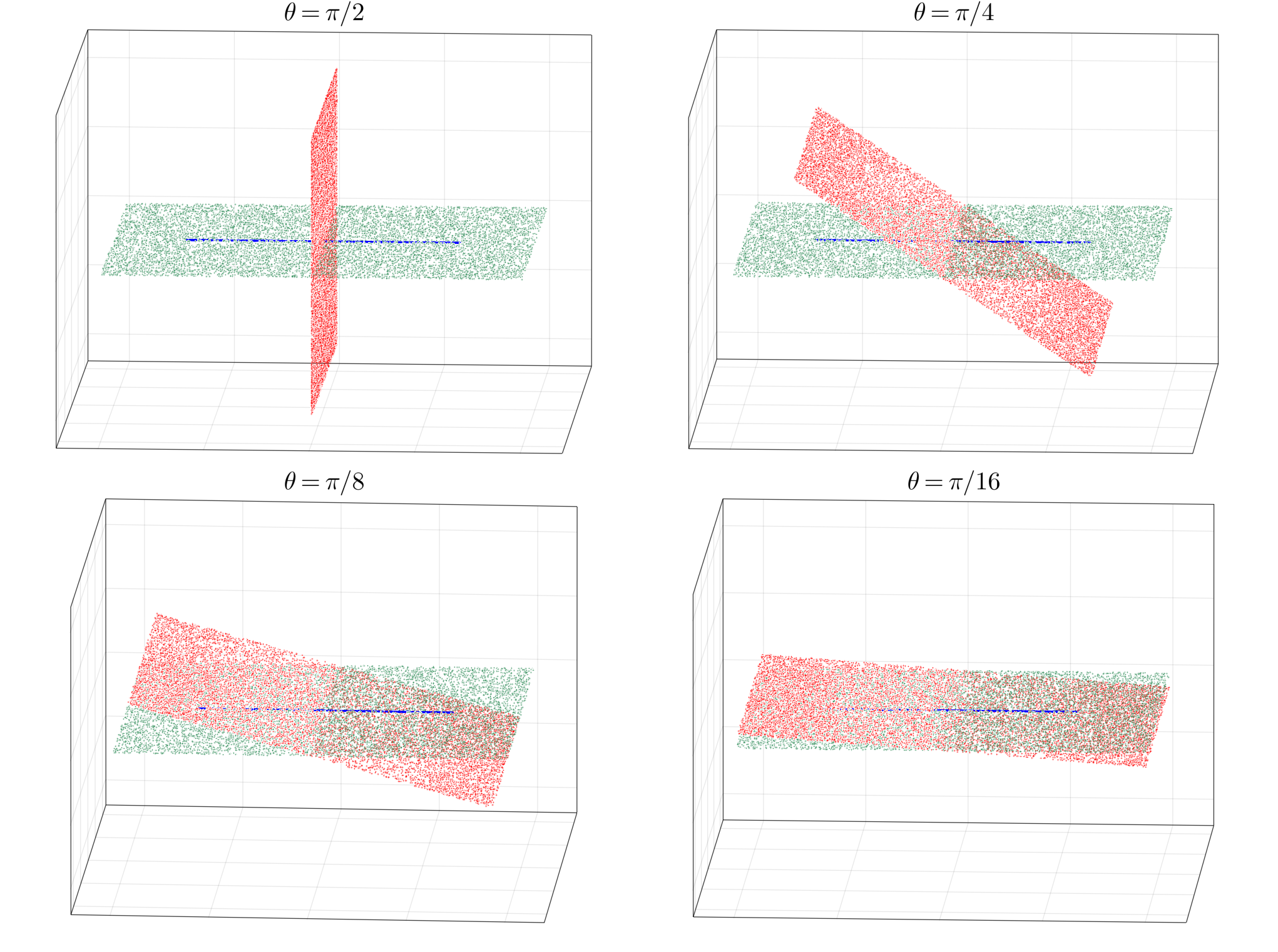
Figure 5. Samples of $\Omega=\Omega_{1}\cup\Omega_{2}$ and $\Gamma$ (blue), where $\Omega_{1}$ (green) and $\Omega_{2}$ (red) have no curvature.

Figure 6. $L_{n,t}f$ evaluated on $\Gamma$. Flat manifolds.

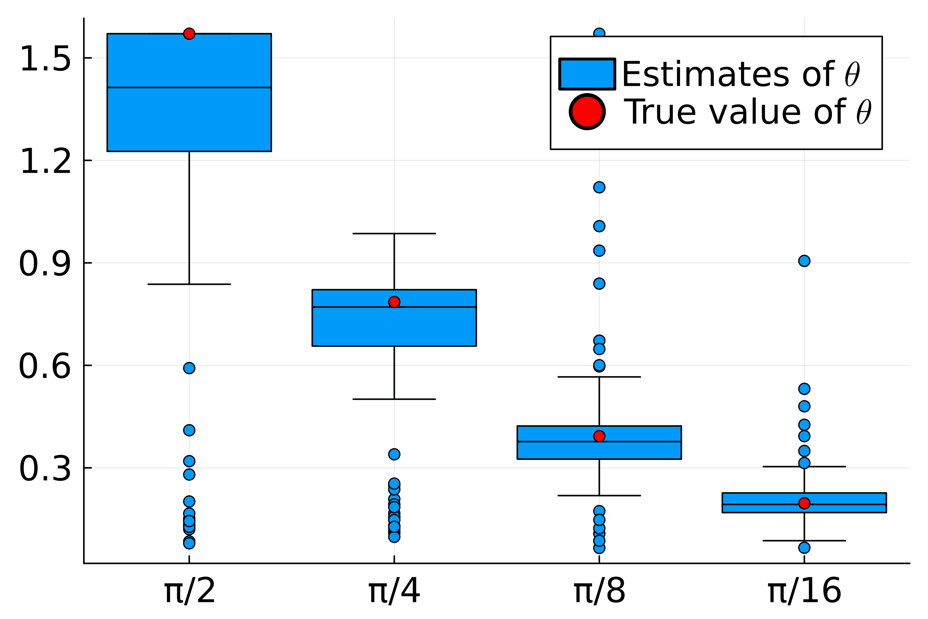
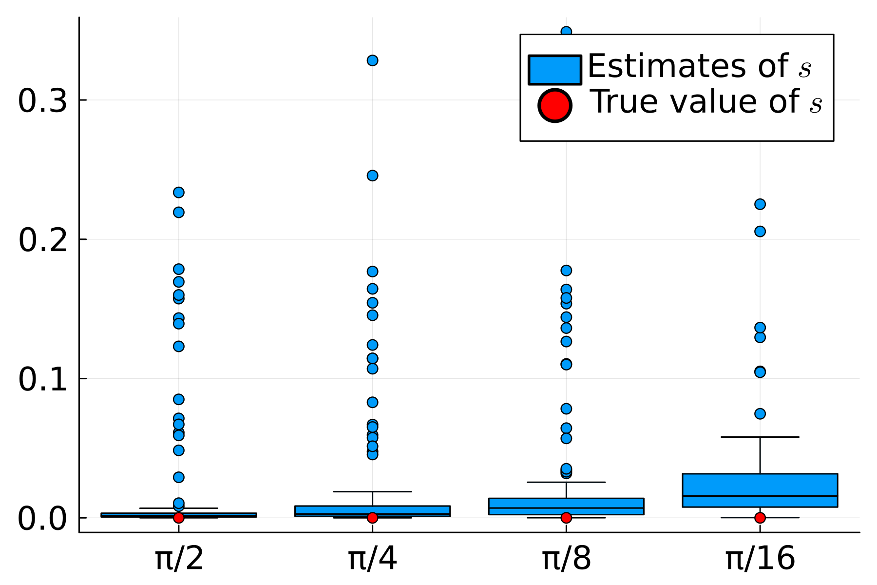
Figure 7. Estimates of $\theta$ and $s$ on flat manifolds.

5.1.3. Curved manifolds

Here we test these methods in the case that $\Omega=\Omega_{1}\cup\Omega_{2}$ is $(L,2R)$-regular, with $L=0.5$ and $R$ having no upper bound. The setup is the same as what we see in Fig. 8.

Using Corollary 4.5 we have that

$$\begin{split}L_{t}f(x_{i})&=t^{d/2+1/2}\widehat{A}(x)v_{n,\Omega_{1}}r\sin\theta e^{-r^{2}\sin^{2}\theta_{1}}+t^{d/2+1/2}\widehat{A}(x)8LR^{2}\\ &\qquad+t^{d/2}C_{L,R}(x)8p\pi^{d/2}+2e^{-r_{0}^{2}}D(x).\end{split}$$

Let us denote $C\coloneqq LR^{2}(1+4LR^{2})+(4LR^{2})^{2}$ and $D\coloneqq\text{diam}(\Omega)$. Then since $\widehat{A}\leq 2\pi^{d/2}$, $C_{L,R}\leq C$ and $\widehat{A}(x)\leq(1+3C)2\pi^{d/2}$, we need that

$$\max_{i}L_{n,t}f(x_{i})>2\left(t^{d/2+1/2}(1+3C)8LR^{2}+t^{d/2}C8p\pi^{d/2}+2e^{-r_{0}^{2}}\right)$$

and

$$\max_{i}L_{n,t}f(x_{i})<-2\left(t^{d/2+1/2}(1+3C)8LR^{2}+t^{d/2}C8p\pi^{d/2}+2e^{-r_{0}^{2}}\right)$$

to be able to say, with some probability that $\Gamma$ intersects $\Omega_{1}\cap\Omega_{2}$. Each term above can be made arbitrarily by making $L$ small and $r_{0}$ large enough.

Remark 5.4.

Since there is curvature, we cannot expect $\theta_{i}=\theta$ for every $i=1,\dots,n$, or even between any pair of them. However, we can still estimate the location of the intersection as before, and estimating $\theta$ in this way provides some information about the intersection, even if it is not as strong as in the case without curvature. The range of possible values for $\theta$, due to curvature, can be bounded by knowing the curvature constant $L$.

In Fig. 8 we see our samples of $\Omega$ and $\Gamma$, in Fig. 9 we see an example of the values we get in $P$. Finally, in Fig. 10 we see how well this approach works in trying to learn both $\theta$ and $r$.

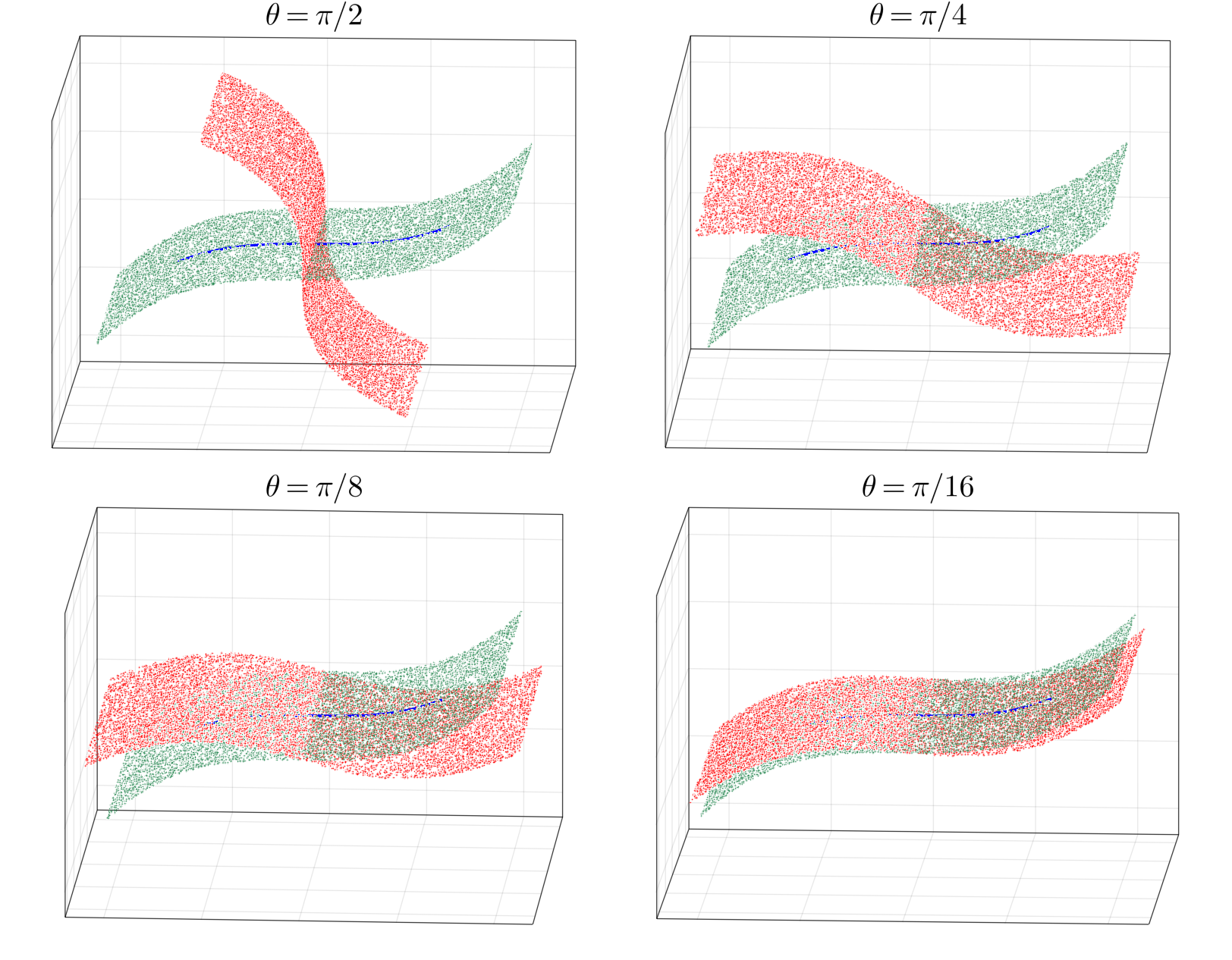
Figure 8. Samples of $\Omega=\Omega_{1}\cup\Omega_{2}$ and $\Gamma$ (blue), where $\Omega_{1}$ (green) and $\Omega_{2}$ (red) have curvature.

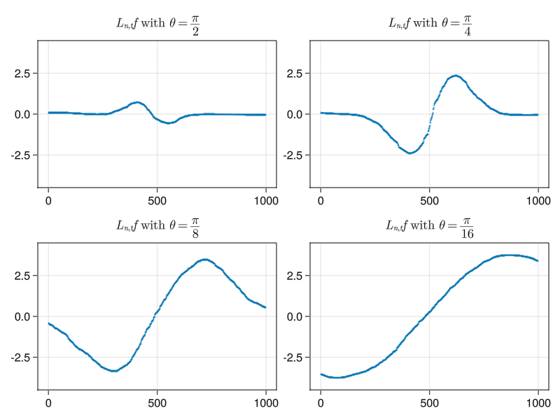
Figure 9. $L_{n,t}f$ evaluated on $\Gamma$. Curved manifolds.

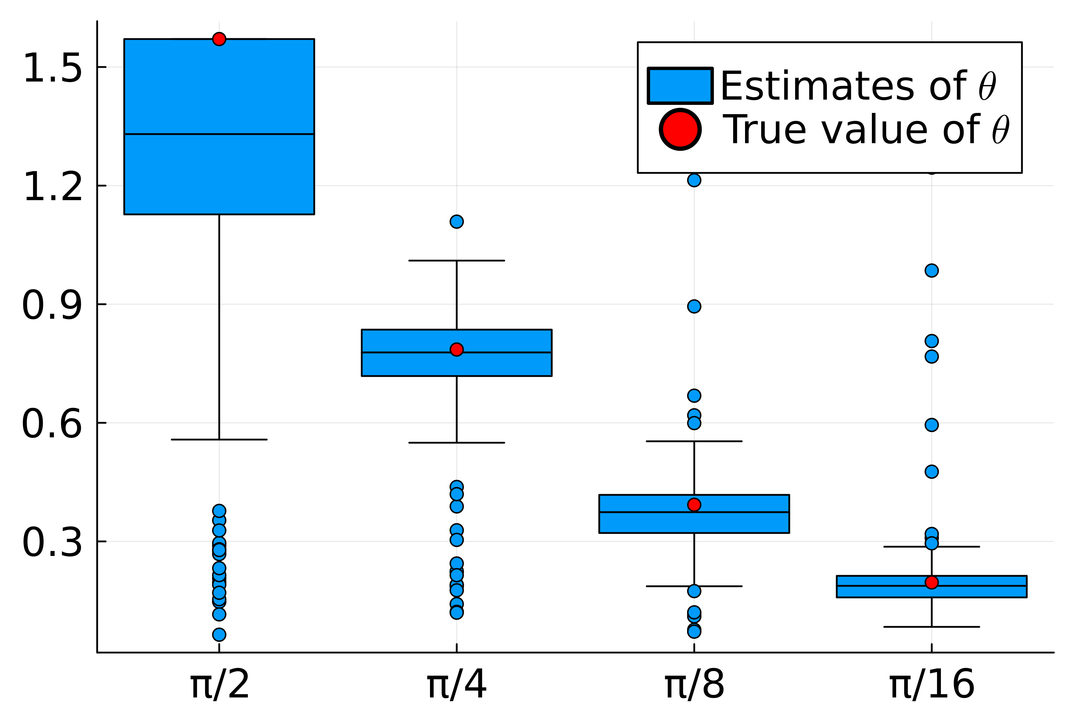
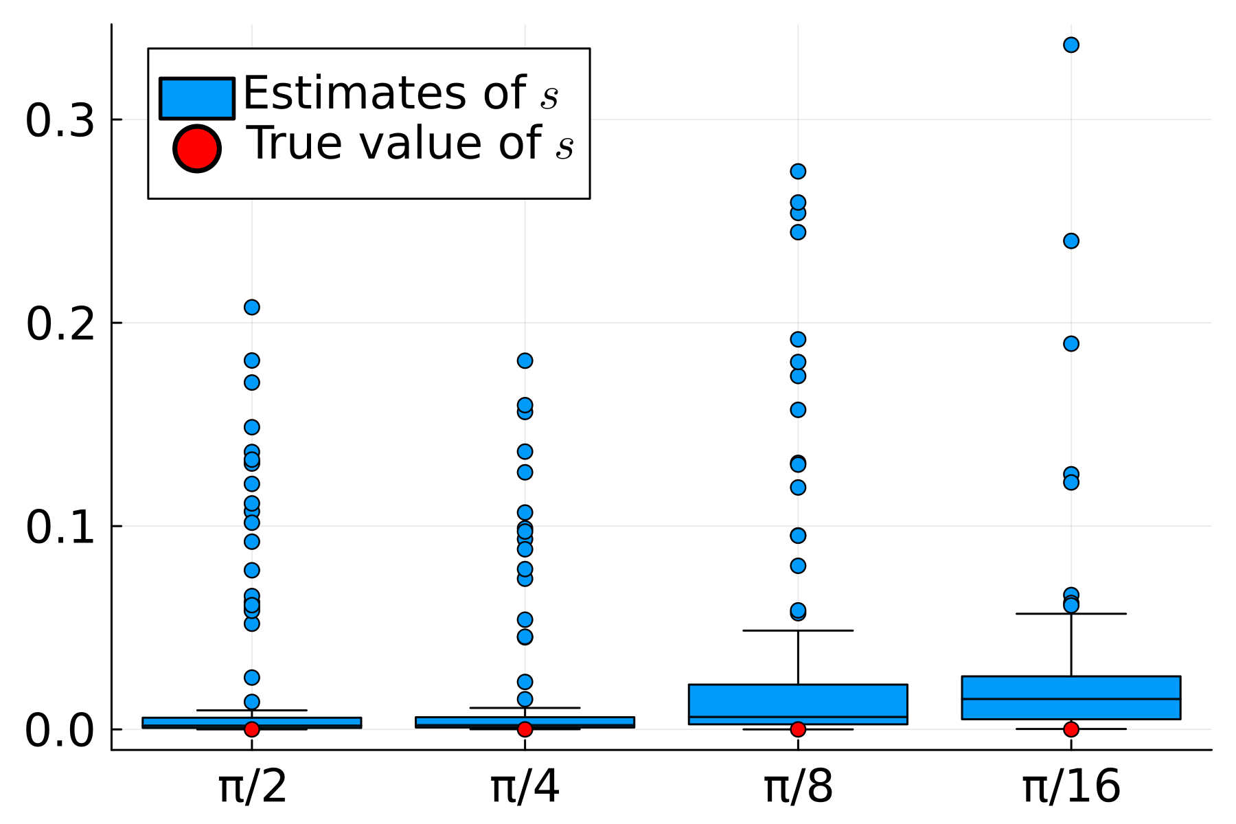
Figure 10. Estimates of $\theta$ and $s$ on curved manifolds.

6. Final remarks

In this paper we built upon the work of [2] and developed explicit versions of their asymptotic analysis of $x\to L_{t}f(x)$. Our results are the strongest and most useful in the case of flat manifolds, and the motivation to focus on this scenario comes partly from Remark 4.1.

While the bounds in Theorem 3 are weaker, our numerical experiments suggest that this approach can be useful for gaining geometric information about the union of more general manifolds $\Omega=\cup_{i}\Omega_{i}$. In [2], the authors mainly considered sets $\Omega=\cup_{i=1}^{n}\Omega_{i}$ with $n\leq 2$. Our approach of splitting $L_{t}$ into components $L_{t}^{i}$ makes it easy to directly apply our theorems for $n\geq 2$, allowing us to consider a wider range of singularities. For example, we can extend the framework to examine points that are both of Type 1 and Type 2, or to study intersections of more than two manifolds. A drawback of this approach is that the error terms are compounded when they are just added together for each $L_{i}^{t}$, but whether this is a problem will depend on the specific application.

In our numerical experiments, we assumed that $\Omega=\cup_{i=1}^{2}\Omega_{i}$ and had access to samples of a continuous curve $\Gamma$, which allowed us to estimate geometric properties near intersections. Future work could involve extending our framework to other types of singularities and developing similar tests and estimators. It would also be interesting to explore methods that do not rely on direct access to such curves.

Similar theorems can be proven for other kernels besides the Gaussian one, as many ideas used in our proofs are not specific to the Gaussian case, but rather rely mainly on symmetries of $K_{t}$. Investigating the use of other kernels and comparing their performance in different scenarios is a promising direction for future research.

References

- [1] M. Belkin and P. Niyogi, “Towards a theoretical foundation for laplacian-based manifold methods,” Journal of Computer and System Sciences, vol. 74, no. 8, pp. 1289–1308, 2008.
- [2] M. Belkin, Q. Que, Y. Wang, and X. Zhou, “Toward understanding complex spaces: Graph laplacians on manifolds with singularities and boundaries,” in Conference on learning theory, pp. 36–1, JMLR Workshop and Conference Proceedings, 2012.
- [3] M. Belkin and P. Niyogi, “Laplacian eigenmaps and spectral techniques for embedding and clustering,” Advances in neural information processing systems, vol. 14, 2001.
- [4] R. Kannan, S. Vempala, and A. Vetta, “On clusterings: Good, bad and spectral,” Journal of the ACM (JACM), vol. 51, no. 3, pp. 497–515, 2004.
- [5] U. v. Luxburg, O. Bousquet, and M. Belkin, “On the convergence of spectral clustering on random samples: the normalized case,” in International Conference on Computational Learning Theory, pp. 457–471, Springer, 2004.
- [6] J. Shi and J. Malik, “Normalized cuts and image segmentation,” IEEE Transactions on pattern analysis and machine intelligence, vol. 22, no. 8, pp. 888–905, 2000.
- [7] A. Ng, M. Jordan, and Y. Weiss, “On spectral clustering: Analysis and an algorithm,” Advances in neural information processing systems, vol. 14, 2001.
- [8] M. Belkin and P. Niyogi, “Laplacian eigenmaps for dimensionality reduction and data representation,” Neural computation, vol. 15, no. 6, pp. 1373–1396, 2003.
- [9] B. Nadler, S. Lafon, R. R. Coifman, and I. G. Kevrekidis, “Diffusion maps, spectral clustering and reaction coordinates of dynamical systems,” Applied and Computational Harmonic Analysis, vol. 21, no. 1, pp. 113–127, 2006.
- [10] M. Belkin and P. Niyogi, “Semi-supervised learning on riemannian manifolds,” Machine learning, vol. 56, no. 1, pp. 209–239, 2004.
- [11] M. Belkin and P. Niyogi, “Convergence of laplacian eigenmaps,” Advances in neural information processing systems, vol. 19, 2006.
- [12] O. Bousquet, O. Chapelle, and M. Hein, “Measure based regularization,” Advances in Neural Information Processing Systems, vol. 16, 2003.
- [13] S. S. Lafon, Diffusion maps and geometric harmonics. Yale University, 2004.
- [14] J. R. Munkres, Analysis on manifolds. CRC Press, 2018.
- [15] W. Gabcke, Neue Herleitung und explizite Restabschätzung der Riemann-Siegel-Formel. PhD thesis, Georg-August-Universität Göttingen, 1979.