Dimensions of exactly divergence-free finite element spaces in 3D

Abstract.

We examine the dimensions of various inf-sup stable mixed finite element spaces on tetrahedral meshes in 3D with exact divergence constraints. More precisely, we compare the standard Scott–Vogelius elements of higher polynomial degree and low order methods on split meshes, the Alfeld and the Worsey–Farin split. The main tool is a counting strategy to express the degrees of freedom for given polynomial degree and given split in terms of few mesh quantities, for which bounds and asymptotic behavior under mesh refinement is investigated. Furthermore, this is used to obtain insights on potential precursor spaces in full de Rham complexes for finite element methods on the Worsey–Farin split.

1. Introduction

Mixed finite element spaces for the Stokes and Navier–Stokes equations have been developed and investigated since the 70s, see, e.g., [TH73, CR73, ABF84, BR85, SV85] and [BBF13] for a review. Inf-sup stability [BS08] of the mixed pair of finite element spaces is a necessary condition to ensure well-posedness and stability of the discrete solutions. However, in general inf-sup stable pairs do not lead to exactly divergence-free discrete velocity functions, which is the case for most classical mixed pairs like the Taylor–Hood [TH73], the Crouzeix–Raviart [CR73], the MINI [ABF84], and the Bernardi–Raugel [BR85] elements. Yet, exact incompressibility constraints are beneficial for example for pressure robust approximation [JLMNR17]. The class of mixed finite element spaces with exact divergence constraints has been reviewed by Neilan in [Nei20]. As noted therein, in three dimensions only a few inf-sup stable pairs of spaces with exact divergence-constraints are available, and the analysis of such methods is still far from complete.

In the following we consider an open bounded domain $\Omega\subset\mathbb{R}^{3}$ with polytopal boundary $\partial\Omega$. Throughout, ${\mathcal{T}}$ denotes a conforming tetrahedral triangulation (or mesh) into closed tetrahedra of $\overline{\Omega}\subset\mathbb{R}^{3}$ in the sense of Ciarlet [Cia02, Sec. 2.1]. This is then a pure simplicial $3$-complex in the language of algebraic topology.

We consider pairs of finite element spaces consisting of

• a velocity space ${\bf V}_{k}({\mathcal{T}})\subset C(\overline{\Omega})$, which is the space of continuous vector-valued functions that are piecewise polynomials of degree at most $k$ on the mesh ${\mathcal{T}}$, and

• a pressure space ${{\nabla\cdot}\,}{\bf V}_{k}({\mathcal{T}})\subset L^{\infty}(\Omega)$ which is a subspace of $\Pi_{k-1}({\mathcal{T}})$, the space of discontinuous piecewise polynomials of degree at most $k-1$ on the same tetrahedral mesh,

for $k\geq 1$. Since the pressure space is the divergence of the velocity space, discretely divergence-free velocity functions are indeed exactly divergence-free. Also, for both the inf-sup condition to be satisfied and the discretely divergence-free velocity functions to be exactly divergence-free, the pressure space necessarily has to be the space of divergence of the velocity functions, cf. [Nei20]. Starting from this ansatz the challenge is to characterize the pressure space.

The 2D version of these elements are the Scott–Vogelius elements [SV85, SV85a, GS19]. For those elements on general meshes ${\mathcal{T}}$ the pressure space can be locally characterized by considering the so-called singular vertices. Those are vertices that have (only) adjacent edges that lie on two straight lines. Furthermore, they are known to be inf-sup stable for polynomial degrees $k\geq 4$, see [GS19]. In 3D the situation is more challenging: the pressure spaces have not been characterized and inf-sup stability is available only in special cases. More specifically, it has been proved in [Zha11] that in 3D on a particular family of regular meshes ${\mathcal{T}}_{h}$, the so-called Freudenthal triangulations [Bey00], the pair $({\bf V}_{k}({\mathcal{T}}_{h}),{{\nabla\cdot}\,}{\bf V}_{k}({\mathcal{T}}_{h}))$ satisfies the inf-sup condition for polynomial degrees $k\geq 6$. Recent computational experiments on this family of regular meshes [FMS22] suggest that the inf-sup condition holds for $k\geq 4$ with constant independently of the mesh size $h$.

For the purpose of minimizing the dimension of the discrete problem there has been significant interest in spaces of lower polynomial degree. To achieve inf-sup stability for standard piecewise polynomial functions for lower polynomial degree $k$ split meshes have been considered, cf. [Zha05, Zha11a, FGNZ22] and the review in [Nei20]. Even though the lower-order methods on split meshes are essentially the Scott–Vogelius method on a special mesh, for clarity we shall refer to them by the name of the split. Only to the elements on the original mesh we refer to as Scott–Vogelius elements. Notably, the split methods do not involve macro-elements in the usual sense.

Here we show that in 3D the discrete spaces for all but one low-order method on split meshes considered to date have a substantially larger dimension than the 3D version of the Scott–Vogelius method using $({\bf V}_{k}({\mathcal{T}}),{{\nabla\cdot}\,}{\bf V}_{k}({\mathcal{T}}))$ for $k=4$ on the original mesh. Even for $k=6$, this pair has only at most 50% higher dimension than most of the lowest-order split methods considered here. The only exception of this is the lowest order case on the so-called Worsey-Farin split mesh. By comparing the actual number of degrees of freedom rather than the polynomial degree, we find that the Scott–Vogelius method is competitive or at least not much more costly than standard low-order methods. Also this argument has not even taken into account the improved approximability results available for higher order finite element spaces. It is notable that the only method that is more efficient is the lowest order method. As soon as one considers methods of higher order than linear order the Scott–Vogelius element for $k=4$ is the most efficient (by a factor $2$).

Our observations suggest that there is need for further investigation of the Scott–Vogelius element in three dimensions. In particular insights into meshes with singularities are of interest, i.e., meshes for which ${{\nabla\cdot}\,}{\bf V}_{k}({\mathcal{T}})$ is a strict subspace of $\Pi_{k-1}({\mathcal{T}})$. Note that nearly singular meshes, that is meshes that are very close to singular meshes, typically have a large inf-sup constant leading to degraded performance [BS08, Sco18].

We limit our attention to methods that use a Lagrange space on the original or on some split mesh as velocity space and the divergence thereof as pressure space. Note however, that outside of this class there are alternative elements satisfying exact divergence-constraints, see, e.g., [FN13, GN14a, GN14]. Hence they are suited for pressure robust approximation, cf. [JLMNR17], and it would be of interest to compare the computational cost of these schemes as well.

Our main tool for determining the number of degrees of freedom of the respective finite element spaces is a counting argument for mesh quantities in 3D. Similar methods have been applied in [Nei20] to show surjectivity of a discrete divergence operator and hence to prove discrete inf-sup stability. Furthermore, the author of [Nei20] has used such arguments to obtain insights into discrete de Rham complexes. The numbers of tetrahedra, faces, edges and vertices in a mesh can be expressed in just two parameters, for example the number of vertices and the average number of edges emanating from each vertex in the mesh. On the latter we obtain estimates. Furthermore, under uniform mesh refinement their asymptotic behavior is investigated in [PR03, PR05], which we shall review. Indeed, for a range of uniform mesh refinements the average mesh quantities converge to the ones attained by certain regular meshes, as the mesh is refined. This includes the 3D red refinement [Bey95, Zha95, MW95], bisection refinement such as the generalization of the newest vertex bisection [Bän91, Kos94] as well as the longest edge bisection [Riv91], and the Carey-Plaza algorithm [PC00]. Consequently, at least for large meshes we obtain estimates for the mesh quantities and then also on the number of degrees of freedom in the finite element spaces under consideration.

The corresponding results in 2D are much simpler and will be provided for comparison.

Outline

In section 2 we review mesh splits available in the literature both in 2D and in 3D. For general 3D tetrahedral conforming meshes we present an approach to count the mesh quantities in section 3. The resulting formulæ involve the average number $\overline{e}$ of edges adjacent to a vertex in the mesh. We derive bounds and review its behavior under certain mesh refinements to determine realistic values of $\overline{e}$. Applying the counting methods allows us to determine the dimensions of various mixed finite element pairs in section 4. Furthermore, applying the counting strategy yields insights into the de Rham complex for the Worsey–Farin split presented in section 5. Finally, section 6 summarizes our conclusions.

2. Split meshes

There is a number of split meshes that allow for exact divergence constraints to be satisfied for low-order finite elements on them. Perhaps the earliest such method uses the two-dimensional Malkus crossed-triangle mesh [MH78, MO84], which is based on subdividing quadrilaterals into four triangles and uses piecewise linear velocity functions. The Malkus crossed-triangle split introduces singular vertices [MS75, SV85, SV85a] at the cross-points in the center of each quadrilateral. Since then a range of split-mesh methods have been developed for simplicial triangulations with the aim to achieve inf-sup stability for low polynomial degrees, see [Nei20] for a review. Let us summarize the split methods leading to exact divergence constraints which we investigate in the following. To motivate and clarify the discussion we shall begin with the two-dimensional situation and then proceed with the three-dimensional situation.

2.1. Splits in 2D

There are two ways of splitting a triangle $\tau$.

The Alfeld split (sometimes referred to as barycentric split) splits each triangle into three triangles and creates one new vertex. This is done by choosing one interior point, e.g., the barycenter of $\tau$, and introducing three edges that connect each vertex of $\tau$ with this interior point. The Alfeld split eliminates any singular or nearly singular vertices, cf. [AQ92].

The Powell–Sabin split [PS77, GLN20] splits each triangle $\tau$ into six triangles and is a refinement of the Alfeld split. Starting from an Alfeld split each triangle is split again by connecting the interior points of any two triangles in the original mesh that share an edge. This results in a total of six new edges in the interior of $\tau$. It creates collinear edges in any two edge-adjacent triangles, and thus introduces singular vertices at the intersection of the original edges with the newly introduced edges. One advantage of the Powell–Sabin split is that the angles of the resulting triangulation are more favorable than the ones in the Alfeld split, since large angles are bisected. Nevertheless, the Powell–Sabin split reduces the angles in the original triangulation.

Lemma 1 (mesh quantities for 2D split meshes).

Let ${\mathcal{T}}$ be a conforming simplicial triangulation of a polyhedral bounded domain $\Omega\subset\mathbb{R}^{2}$ with $V$ vertices, $E$ edges and $T$ triangles. Let ${\mathcal{T}}_{{A}}$ be the Alfeld split and ${\mathcal{T}}_{{P}}$ the Powell–Sabin split of ${\mathcal{T}}$. Then we have the following:

1. ${\mathcal{T}}_{{A}}$ has $V_{A}=V+T$ vertices, $E_{A}=E+3T$ edges, and $T_{A}=3T$ triangles.

2. ${\mathcal{T}}_{{P}}$ has $V_{P}=V+E+T$ vertices, $E_{P}=2E+6T$ edges, and $T_{P}=6T$ triangles.

2.2. Splits in 3D

For a tetrahedron $\tau$ there are even more variants of barycentric subdivisions, some of which are the following.

The Alfeld split [AS05, Zha05, GN18] splits each tetrahedron in the mesh into $4$ tetrahedra. This is achieved by introducing $4$ new edges in any tetrahedron $\tau$, shown as gray dashed lines in Figure 1 (left), that connect each vertex of $\tau$ to an interior point, e.g., its barycenter. This creates one new vertex per tetrahedron. One defect of the Alfeld split is that it does not commute with a multigrid subdivision. However, an optimal-order convergent, non-nested multigrid method has been developed in [FMSW21].

The Worsey–Farin split [WF87] (also sometimes referred to as Clough–Tocher or Powell–Sabin [Zha11a, Nei20]) is a refinement of the Alfeld split and subdivides each of the $4$ subtetrahedra in the Alfeld split into $3$ subtetrahedra. Figure 1 (right) depicts this further split, where the subtetrahedra of the Alfeld split are detached for the purpose of visualization. Each face of the original mesh is subdivided via a 2D Alfeld split resulting in one new vertex per face and $3$ new edges per face. The splitting point of the 2D Alfeld split of a face can be chosen as the point on the connecting line of the interior points of the two face neighboring tetrahedra, cf. [FGNZ22]. Then the face splitting point is connected to the interior point of the original simplex, resulting in $4$ new edges per tetrahedron in the Alfeld split. In this way, the original tetrahedron is divided into $12$ subtetrahedra.

Applying these splits to each tetrahedron in the triangulation ${\mathcal{T}}$ leads to new triangulation, denoted by ${\mathcal{T}}_{{A}}$ for the Alfeld split and by ${\mathcal{T}}_{{W}}$ for the Worsey–Farin split. This creates on each face of the original mesh three singular edges, that is edges whose adjacent faces are lying (only) in two planes [FGNZ22, Def. 4.1].

Alternatively, we may consider a barycentric subdivision of each $\tau$ into $24$ subtetrahedra. Since this subdivision is a natural generalization of the Powell–Sabin split to three dimensions, it has been referred to as a generalized Powell–Sabin split [WP88].

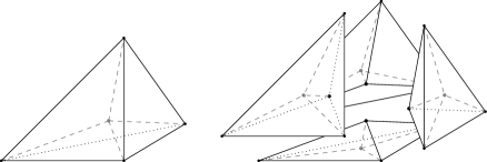
Figure 1. Alfeld split into $4$ new tetrahedra (left) and Worsey–Farin split into $3$ new tetrahedra each (right) in 3D with the new edges (dashed) and new vertices in gray. For simpler visualization the $4$ tetrahedra resulting from the Alfeld split are detached in the right-hand figure.

Lemma 2 (mesh quantities for 3D split meshes).

Let ${\mathcal{T}}$ be a conforming simplicial triangulation of a polyhedral bounded domain $\Omega\subset\mathbb{R}^{3}$ with $V$ vertices, $E$ edges, $F$ faces and $T$ tetrahedra. Let ${\mathcal{T}}_{{A}}$ be the Alfeld split and ${\mathcal{T}}_{{W}}$ the Worsey-Farin split of ${\mathcal{T}}$.

1. ${\mathcal{T}}_{{A}}$ has $V_{A}=V+T$ vertices, $E_{A}=E+4T$ edges, $F_{A}=F+6T$ faces and $T_{A}=4T$ tetrahedra.

2. ${\mathcal{T}}_{{W}}$ has $V_{W}=V+F+T$ vertices, $E_{W}=E+8T+3F$ edges, $F_{W}=3F+18T$ faces and $T_{W}=12T$ tetrahedra.

3. Mesh quantities in 3D

Using counting arguments we want to express all mesh quantities in just a few quantifiable parameters, the values of which we aim to investigate and estimate. In the following section we use those insights to compare the dimensions of mixed finite element spaces.

The starting point are the well-known Euler characteristics both for the closed domain $\overline{\Omega}$ as well as for its boundary $\partial\Omega$, cf. [Eul58, Hat02]. Let $V$ be the number of vertices, $E$ the number of edges, $F$ the number of faces and $T$ the number of tetrahedra in ${\mathcal{T}}$. Furthermore, we denote the corresponding number of mesh quantities on the boundary by $V_{b},E_{b}$ and $F_{b}$, respectively. Then, there exist constants $\chi,\chi_{b}\in\mathbb{Z}$ such that

(1) $$V-E+F-T=\chi\qquad\text{ and }\qquad V_{b}-E_{b}+F_{b}=\chi_{b}.$$

The constants $\chi,\chi_{b}\in\mathbb{Z}$ are topological invariants that only depend on the genus of the domain $\overline{\Omega}$. For example, for $\overline{\Omega}$ simply connected one has $\chi=1$ and $\chi_{b}=2$. This can be shown by induction starting from a single tetrahedron.

Additionally, some simple combinatorical arguments show that

(2) $$2F-F_{b}=4T\qquad\text{ and }\qquad 3F_{b}=2E_{b}.$$

The proof follows similarly as in the 2D case [MS75]. Imagine placing $2$ marbles on each interior face and one on each boundary face. Now move the marbles into the neighboring tetrahedra. Thus each tetrahedron will have $4$ marbles, since it has $4$ faces. In total we have allocated $2F-F_{b}$ marbles to tetrahedra, and we end up with $4T$. By the conservation of marbles, the first equality in (2) is proved. The proof of the second identity follows analogously. We put $3$ marbles on each boundary face, then move them to the boundary edges. After the transfer each boundary edge has $2$ marbles.

Remark 3 (2D case).

In 2D one can express all mesh quantities $V,E,T$ ($T$ denotes the number of triangles) and $V_{b},E_{b}$ in terms of only $V$ and $V_{b}$. Indeed, the Euler characteristics are

(3) $$V-E+T=\chi\qquad\text{ and }\qquad V_{b}-E_{b}=\chi_{b},$$

and the combinatorical identity

(4) $$3T=2E-E_{b}.$$

suffices. From those it follows that

$$E =3V-V_{b}-3\chi+\chi_{b},\qquad\quad E_{b} =V_{b}-\chi_{b},$$

$$T =2V-V_{b}-2\chi+\chi_{b}.$$

For a simply connected domain we further have that $\chi_{b}=0$ and $\chi=1$.

In 3D the identities (1) and (2) are not enough to express all mesh quantities in the number of vertices $V$ and $V_{b}$. In this case we need to choose an additional parameter.

3.1. Average number of edges

Additionally to $V,V_{b}$ we consider the average number of edges intersecting in a vertex. In principle we could use alternative (average) quantities, cf. Remark 8 below, but we shall see in the sequel that this choice has some advantages.

Let $e_{i}$ denote the number of edges emanating from vertex $v_{i}$ in ${\mathcal{T}}$, for $i=1,\ldots,V$. Then we define the arithmetic mean

(5) $$\overline{e}\coloneqq\frac{1}{V}\sum_{i=1}^{V}e_{i}=\frac{2E}{V},$$

where the second identity holds since summing $e_{i}$ over all $i$ counts every edge twice. Thus $\overline{e}$ is the average number of edges emanating from vertices in a mesh ${\mathcal{T}}$.

Proposition 4.

Let ${\mathcal{T}}$ be a conforming simplicial triangulation with $V$ vertices, $E$ edges, $F$ faces and $T$ tetrahedra of a domain $\Omega\subset\mathbb{R}^{3}$ as above with topological constants $\chi,\chi_{b}$, cf. (1). Then, the mesh quantities can be expressed in terms of $V,V_{b}$ and $\overline{e}$, as

$$E =\tfrac{1}{2}\overline{e}V,\qquad\qquad E_{b} =3(V_{b}-\chi_{b}),$$

$$F =\left(\overline{e}-2\right)V-V_{b}+2\chi+\chi_{b},\qquad\quad F_{b} =2(V_{b}-\chi_{b}),$$

$$T =\left(\tfrac{1}{2}\overline{e}-1\right)V-V_{b}+\chi+\chi_{b}.$$

Proof.

The expression for $E$ follows by the definition of $\overline{e}$. From (2) we have that $F_{b}=\tfrac{2}{3}E_{b}$ and applying it in the equation for the boundary quantities in (1) yields

$$E_{b}=3(V_{b}-\chi_{b})\quad\text{ and }\quad F_{b}=2(V_{b}-\chi_{b}).$$

Inserting the expression for $F_{b}$ in the first identity in (2) and using the expression of $\overline{e}$ in the first identity in (1) leads to

$$F-2T =2(V_{b}-\chi_{b}),$$

$$F-T =\chi-V+\tfrac{1}{2}\overline{e}V.$$

Solving the system of equations for $F$ and $T$ proves the identities as stated. ∎

Remark 5.

If for a fixed domain $\Omega\subset\mathbb{R}^{3}$ the mesh quantities in the mesh ${\mathcal{T}}$ are sufficiently large one may neglect the asymptotically smaller quantities $\chi,\chi_{b}$ and $V_{b}$. Then, one arrives at

(6) $$E=\tfrac{1}{2}\overline{e}V,\qquad F\approx(\overline{e}-2)V,\qquad\text{ and }\quad T\approx\left(\tfrac{1}{2}\overline{e}-1\right)V.$$

Before investigating general bounds on $e_{i}$ and $\overline{e}$ let us consider the values for special meshes.

Example 6 (star meshes).

We consider a simply connected open $\Omega\subset\mathbb{R}^{3}$ and meshes with a single interior vertex $v_{1}$. In this situation $\partial\Omega$ is a polyhedral surface topologically equivalent to a 2-sphere $(\chi=1,\chi_{b}=2)$ and the one interior vertex is connected to each vertex on the boundary, i.e., one has that

$$V_{b}=e_{1},\qquad V=V_{b}+1\quad\text{ and }\quad E=E_{b}+V_{b}.$$

These triangulations can be viewed as the star of an interior vertex for general triangulations, and quantities associated with them will be relevant in subsequent derivations.

The simplest example is the domain and mesh ${\mathcal{T}}$ arising from the Alfeld split of one single tetrahedron. In this case we have that $V_{b}=4=e_{1}$, $V=5$ and $E=10$.

This is indeed the smallest such mesh in the sense that general star meshes of the type as described satisfy $e_{1}=V_{b}\geq 4$, and $E\geq 10$ as we shall show now. Using the fact that each boundary vertex has at least $3$ adjacent boundary edges and there is at least one boundary vertex it follows that $F_{b}\geq 3$. From the expressions in Proposition 4 we have that $F_{b}=2(V_{b}-2)$ and $E_{b}=3(V_{b}-2)$, since $\chi_{b}=2$. Hence, it follows that $V_{b}=F_{b}/2+2>3$ and thus $V_{b}\geq 4$, since $V_{b}\in\mathbb{N}$. Then it also follows that $E_{b}=3(V_{b}-2)\geq 6$ and that $E=E_{b}+V_{b}\geq 10$.

For any given domain $\Omega$ the number $e_{1}=V_{b}$ can be arbitrarily large for suitably chosen meshes. Note however, that for increasing $V_{b}$ the shape regularity of the mesh deteriorates. Indeed, $e_{1}$ can be bounded above by the shape regularity constant or minimum solid angle, as stated in Lemma 13 below.

However, $\overline{e}$ cannot be arbitrarily large, since we take the mean over all vertices. Recalling that $V=V_{b}+1$, $E=E_{b}+V_{b}$ and that $E_{b}=3(V_{b}-2)$, we obtain

$$\overline{e}=\frac{2E}{V}=\frac{8V_{b}-12}{V_{b}+1}.$$

This expression is strictly growing in $V_{b}$ and bounded above by $8$. Since we have $V_{b}\geq 4$ by the above arguments, we find that

$$4\leq\overline{e}\leq 8\quad\text{ for any }V_{b}\geq 4.$$

The boundary vertices with fewer edges emanating from them are responsible for $\overline{e}$ being bounded.

Example 7 (regular meshes).

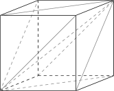
a Kuhn triangulation of a single cube into 6 tetrahedra [Kuh60].

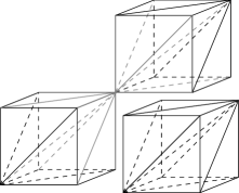
b Two Kuhn cubes sharing a vertex, together with a third Kuhn cube ready to be attached.

Figure 2. Regular triangulation of a cube and combination of those to form the triangulation of a rectangular domain.

The so-called Kuhn triangulation [Kuh60, Bey00] is a regular triangulation of the unit cube in $\mathbb{R}^{d}$. For dimension $d=3$ it consists of $6$ tetrahedra. In this case it has one interior edge and, for each vertex, it has 3 axis-parallel edges and 3 edges lying on faces, as indicated in Figure 2a. Thus there are 7 edges impinging on each of the vertices at the lower-left and upper-right of the cube.

We refer to a triangulation consisting of Kuhn cubes as Freudenthal triangulation, cf. [Fre42, Bey00].

1. For a mesh of $\mathbb{R}^{3}$ arising by filling the space by Kuhn cubes for every vertex one has that $e_{i}=14$. Indeed, in Figure 2b we see two Kuhn cubes sharing a vertex, with a third cube in position to be added to the complex. In adding the new cube, no new edges are added, and this holds for all six positions where a cube is added to form a space filling triangulation. All edges of the shared vertex are contained already in the two diagonal Kuhn cubes and thus we have that $e_{i}=2\cdot 7=14$, for all $i$.

The quantity $\overline{e}$ is defined only for finite meshes, so we now consider finite subsets of the Freudenthal triangulation based on Kuhn cubes. We can then talk about a limiting value for $\overline{e}$ as the number of cubes tends to infinity.

1. For a bounded rectangular domain $\Omega\subset\mathbb{R}^{3}$ and a regular mesh thereof consisting of $n\cdot m\cdot\ell$ Kuhn cubes we have $e_{i}=14$ only for interior vertices. The boundary vertices have fewer adjacent edges, and hence one has that $\overline{e}\leq 14$. For $m,n,\ell\to\infty$ it follows that $\overline{e}\to 14$, since the number of boundary edges and vertices are asymptotically smaller than the number of interior edges and vertices.

In view of the following remark one could chose any other average quantity instead of $\overline{e}$ as defined in (5) to fully determine all other parameters. However, we prefer to work with the lowest dimensional quantities since they are the simplest to determine by computational means.

Remark 8 (alternative quantities).

For an interior vertex $v_{i}$ in ${\mathcal{T}}$ we can relate the number $e_{i}$ of edges emanating from $v_{i}$ to the number $t_{i}$ of simplices intersecting in $v_{i}$ and the number of faces $f_{i}$ intersecting in $v$. For this it suffices to consider the neighboring patch or the star of the vertex $v_{i}$ in ${\mathcal{T}}$, defined by

(7) $$\omega(v_{i})\coloneqq\{\tau\in{\mathcal{T}}\colon v_{i}\in\tau\}.$$

Then $e_{i}$ is the number of boundary vertices and $f_{i},t_{i}$ are the number of the respective boundary quantities. With the same arguments as in Example 6 we find that

(8) $$f_{i}=3(e_{i}-2)\quad\text{ and }\quad t_{i}=2(e_{i}-2),$$

for any interior vertex $v_{i}$. For the global average quantities we obtain

(9) $$\overline{f}\coloneqq\frac{1}{V}\sum_{i=1}^{V}f_{i}=\frac{3F}{V}\quad\text{ and }\quad\overline{t}\coloneqq\frac{1}{V}\sum_{i=1}^{V}t_{i}=\frac{4T}{V}.$$

With Proposition 4 neglecting the boundary quantities and both $\chi$ and $\chi_{b}$ for large meshes, we find that

(10) $$\overline{f}\approx 3(\overline{e}-2)\quad\text{ and }\quad\overline{t}\approx 2(\overline{e}-2).$$

Also the remaining average quantities can be recovered. Denoting by $\theta_{j}$ the average number of tetrahedra intersecting in edge $\mathrm{e}_{j}$ and by $\phi_{j}$ the average number of faces intersecting in edge $\mathrm{e}_{j}$, for $j=1,\ldots,E$, we may define the average quantities

(11) $$\overline{\phi}\coloneqq\frac{1}{E}\sum_{j=1}^{E}\phi_{j}=\frac{3F}{E}\quad\text{ and }\quad\overline{\theta}\coloneqq\frac{1}{E}\sum_{j=1}^{E}\theta_{j}=\frac{6T}{E}.$$

They can be recovered by

(12) $$\overline{\phi}=2\frac{\overline{f}}{\overline{e}}\approx 6\frac{(\overline{e}-2)}{\overline{e}}\quad\text{ and }\quad\overline{\theta}=3\frac{\overline{t}}{\overline{e}}\approx 6\frac{(\overline{e}-2)}{\overline{e}},$$

where the approximate identity refers again to large meshes where we may neglect the boundary quantities, and both $\chi$ and $\chi_{b}$. See also [PR05, Thm. 3.3].

Example 9.

For the regular mesh in Example 7 from $\overline{e}=14$ the remaining average quantities can be deduced using Remark 8, as summarized in Table 1.

(r)[5pt]—c—c—c—c—c——c—c— $\overline{e}$ & $\overline{f}$ $\overline{t}$ $\overline{\phi}$ $\overline{\theta}$
$14$ $36$ $24$ $\frac{36}{7}$ $\frac{36}{7}$

Table 1. Average mesh quantities for regular mesh as in Example 7.

Remark 10 (Average quantities in 2D).

In 2D the quantities $\overline{e},\overline{t}$ are bounded as

$$2\leq\overline{e}\leq 6\qquad\text{ and }\qquad 1\leq\overline{t}\leq 6,$$

and for any sequence of meshes $({\mathcal{T}}_{n})_{n\in\mathbb{N}}$ of a given domain $\Omega\subset\mathbb{R}^{2}$ with $V_{n}\to\infty$, as $n\to\infty$ one has that

$$\overline{e}_{n}\to 6\quad\text{ and }\quad\overline{t}_{n}\to 6,\qquad\text{ as }n\to\infty.$$

This is a direct consequence of Euler characteristics (3), since

$$\overline{e}=\frac{2E}{V}=6-\frac{2V_{b}}{V}-\frac{6\chi}{V}+\frac{2\chi_{b}}{V},$$

cf. Remark 3. In the formulation for simple planar graphs this result can be found, e.g., in [Wes96, Thm. 6.1.23]. Note that the sequence $({\mathcal{T}}_{n})_{n\in\mathbb{N}}$ may arise as an arbitrary refinement of an initial mesh ${\mathcal{T}}_{0}$ and no assumption of shape regularity or specific refinement scheme enters here.

See also [PR02, Thm. 5.1], which states this for the special case of so-called skeleton-regular refinements.

In 3D to obtain bounds on the average quantities and their asymptotic behavior is much more challenging. In fact, different limiting values of $\overline{e}$ may occur depending on the mesh refinement scheme, cf. [PR05, Tab. 3] and the investigation below.

3.2. Lower bounds

Let us first consider lower bounds for $e_{i}$ and $\overline{e}$. Obviously, each vertex $e_{i}$ is contained in at least one tetrahedron, and hence $e_{i}\geq 3$. This implies the first lower bound $\overline{e}\geq 3$. However, this can be improved in most cases.

Lemma 11.

Let ${\mathcal{T}}$ be a conforming simplicial triangulation of an open bounded domain $\Omega\subset\mathbb{R}^{3}$ as above. Then, for any interior vertex $v_{i}\notin\partial\Omega$ the number $e_{i}$ of edges intersecting at the vertex $v_{i}$ is bounded below as

$$e_{i}\geq 4.$$

Furthermore, if $\Omega$ is pathwise connected and ${\mathcal{T}}$ has at least one interior vertex, then we have that

(13) $$\overline{e}\geq 4.$$

Proof.

The estimate $e_{i}\geq 4$ for any interior vertex $v_{i}$ follows by Example 6.

Since $e_{i}\geq 3$ in general and $e_{i}\geq 4$ for interior vertices $v_{i}$ the only vertices that might hamper the lower bound (13) are boundary vertices $v_{i}$ with $e_{i}=3$. For such vertices we can successively remove the unique tetrahedron $\tau_{i}\in{\mathcal{T}}$ with $v_{i}\in\tau_{i}$ from the mesh. Since the open domain $\Omega$ is pathwise connected, every tetrahedron shares at least one face ($3$ vertices and $3$ edges) with the remaining mesh. Hence, by removing $\tau_{i}$ we remove $4-3=1$ vertex and $6-3=3$ edges. After removing $\tau_{i}$, the remaining mesh ${\mathcal{T}}_{1}\coloneqq{\mathcal{T}}\setminus\{\tau_{i}\}$ still covers a pathwise connected closed domain, and hence we may proceed inductively. Indeed, the tetrahedron $\tau\in{\mathcal{T}}$ that shared a face with $\tau_{i}$ shares at least another face with the remaining mesh ${\mathcal{T}}\setminus\{\tau_{i},\tau\}$, because otherwise $\Omega$ would not be pathwise connected.

Note that this inductive process terminates with a simplicial mesh ${\mathcal{T}}^{\prime}\subset{\mathcal{T}}$, since the number of vertices in ${\mathcal{T}}$ is bounded. The triangulation ${\mathcal{T}}^{\prime}$ is not empty, since ${\mathcal{T}}$ has at least one interior vertex and since in this procedure no interior vertex becomes a boundary vertex. By construction any vertex in ${\mathcal{T}}^{\prime}$ satisfies that $e_{i}\geq 4$, and thus $\overline{e}^{\prime}\geq 4$. Denoting by $k$ the number of tetrahedra removed, and hence the number of vertices removed, the triangulation ${\mathcal{T}}^{\prime}$ has $V^{\prime}=V-k$ vertices and $E^{\prime}=E-3k$ edges. Then, it follows that

$$4\leq\overline{e}^{\prime}=\frac{2E^{\prime}}{V^{\prime}}=\frac{2E-6k}{V-k}=\frac{\overline{e}V-6k}{V-k}.$$

Rearranging leads to

$$\overline{e}\geq 4+\frac{2k}{V}\geq 4,$$

which proves the claim. ∎

Remark 12.

The proof also works, if $\overline{\Omega}$ is simply connected, in which case there might be degeneracies in the domain and in the mesh in the following way: There are two parts of the triangulation, that are connected only through a point or only through an edge. However, for the finite element setting such a situation is of lesser relevance and hence we refrain from presenting the proof.

Since the lower bound $4$ is attained by an Alfeld split of a single tetrahedron the estimate (13) is sharp.

3.3. Upper bounds

Let us investigate bounds on $e_{i}$ depending on the shape regularity of ${\mathcal{T}}$. Since using the shape regularity constant yields rather bad bounds let us instead work with the equivalent minimal solid angle condition, see [BKK08].

For any tetrahedron $\tau\in{\mathcal{T}}$, we denote by $\alpha_{\tau,i}\in(0,4\pi)$ the solid angle of $\tau$ with vertex $v_{i}\in\tau$ as apex. This allows us to define the minimal solid angle $\alpha_{i}$ at vertex $v_{i}$ of ${\mathcal{T}}$, for $i=1,\ldots V$, and the minimal solid angle $\alpha_{{\mathcal{T}}}$ in ${\mathcal{T}}$, respectively, by

$$\alpha_{i} \coloneqq\min_{\tau\in\omega(v_{i})}\alpha_{i,\tau},\qquad i=1,\ldots V,$$

$$\alpha_{{\mathcal{T}}} \coloneqq\min_{i=1,\ldots,V}\alpha_{i}.$$

Lemma 13.

Let ${\mathcal{T}}$ be a conforming simplicial mesh of a domain $\Omega\subset\mathbb{R}^{3}$ as above. We assume that ${\mathcal{T}}$ is shape regular with minimal solid angles $\alpha_{i},\alpha_{{\mathcal{T}}}\in(0,4\pi)$ for $i=1,\ldots V$ as defined above. Then, for any vertex $v_{i}$ the number $e_{i}$ of edges intersecting at the vertex $v_{i}$ is bounded above by

$$e_{i}\leq 2+\frac{2\pi}{\alpha_{i}}\leq 2+\frac{2\pi}{\alpha_{{\mathcal{T}}}}.$$

Proof.

Let $\alpha_{i}$ be the minimal solid angle at $v_{i}$ then we can bound the number $t_{i}$ of tetrahedra intersecting in the vertex $v_{i}$ by

$$t_{i}\leq\frac{4\pi}{\alpha_{i}}\leq\frac{4\pi}{\alpha_{{\mathcal{T}}}}.$$

Using (8) for any interior vertex $v_{i}$ in ${\mathcal{T}}$ we find that

$$e_{i}=\tfrac{1}{2}t_{i}+2\leq\frac{2\pi}{\alpha_{i}}+2\leq\frac{2\pi}{\alpha_{\mathcal{T}}}+2.$$

∎

The minimal solid angle of the Freudenthal triangulation in Example  7 is given by $\alpha_{\mathcal{T}}=\frac{\pi}{12}$. This leads to the bound

$$\overline{e}\leq 26.$$

This is much better than the bound one would obtain using the shape regularity constant, but still larger than the value $\overline{e}\leq 14$ obtained in Example 7.

Note that in the Freudenthal triangulation there is no vertex $v_{i}$ with $e_{i}=26$. It correspond to the ’worst’ case, where for all $8$ Kuhn cubes are attached to a point $v$ in such an orientation that all $6$ simplices in each cube are adjacent to $v$.

Remark 14.

For $d$-dimensional simplicial complexes with $f_{i}$ faces of dimension $i=0,\ldots,d$ the $f$-vector of the complex is defined as $(f_{-1},f_{0},\ldots,f_{d})\in\mathbb{N}^{d+2}$ with the convention $f_{-1}=0$, cf. [Zie95, Def. 8.16], or [Sta92]. Note that simplicial triangulations in the context of numerical analysis are nothing else but pure simplicial complexes, i.e., a simplicial complex for which any $n$-face with $n\leq d$ is a subset of a $d$-simplex. This means that results on bounds of the $f$-vectors directly translate to our setting, with $\overline{e}=\frac{2f_{1}}{f_{0}}$. For general simplicial complexes the theorem by Sperner [Spe28], c.f. [Zha95, Lem. 8.29] yields the upper bound

$$\overline{e}\leq V-1.$$

This is a too coarse estimate for our needs.

It may well be that in the fields of graph theory or of algebraic topology better estimates on $\overline{e}$ are available but unknown to the authors.

Asymptotic behavior under uniform mesh refinement

In Example 7 we have seen that the value $\overline{e}=14$ is attained for certain regular meshes. However, the values of the average quantities attained for the regular mesh also appear as limiting values for families of uniformly refined meshes for a large class of refinement algorithms, as proved in a general setting in [PR05, Thm. 3.6]. See also [PR03] for specific refinement schemes. By uniform refinement (opposed to adaptive refinement) we mean that each simplex in the triangulation is refined according to the refinement algorithm under consideration.

For the sake of clarity we shall review the results on the asymptotic behavior of $\overline{e}$ under uniform mesh refinement in Lemma 15 below. This is solely based on techniques in [PR05] and requires only minimal modification of the arguments. Afterwards in Example 17 below we discuss examples of refinement algorithms that satisfy the assumptions.

We consider a uniform mesh refinement scheme $\mathcal{R}$, which when applied to a simplicial conforming mesh ${\mathcal{T}}$ generates a simplicial conforming mesh ${\mathcal{T}}^{\prime}=\mathcal{R}({\mathcal{T}})$ and has the following properties:

1. each tetrahedron in ${\mathcal{T}}$ is split into $8$ tetrahedra, each face is split into $4$ faces and each edge is split into $2$ edges;

2. the vertices in ${\mathcal{T}}^{\prime}$ are exactly the vertices in ${\mathcal{T}}$ and all the midpoints of edges in ${\mathcal{T}}$.

Lemma 15 ([PR05, Thm. 3.6]).

Let $\Omega\subset\mathbb{R}^{3}$ be an open domain as above with ${\mathcal{T}}_{0}$ a conforming simplicial triangulation of $\Omega$. We assume that $\mathcal{R}$ is a (uniform) refinement scheme satisfying (R1) and (R2). Then, for the family of meshes $\{{\mathcal{T}}_{n}\}_{n\in\mathbb{N}}$ generated by ${\mathcal{T}}_{n}=\mathcal{R}({\mathcal{T}}_{n-1})$ for $n\geq 1$, one has that

$$\overline{e}_{n}\to 14,\quad\text{ as }n\to\infty.$$

Proof.

The proof follows [PR05, Thm 3.6] where the asymptotic behavior of $\overline{\theta}$ and $\overline{t}$ is investigated. We present it to make the presentation self-contained. We consider a mesh ${\mathcal{T}}$ with $V$ vertices, $E$ edges, $F$ faces and $T$ tetrahedra. Let ${\mathcal{T}}^{\prime}=\mathcal{R}({\mathcal{T}})$ be the refined mesh with mesh quantities $T^{\prime},F^{\prime},E^{\prime}$ and $V^{\prime}$. Then by the properties (R1), (R2) we obtain

(14) $$T^{\prime}=8T\quad\text{ and }\quad V^{\prime}=V+E.$$

Applying (R1) and the identities (1) and (2) to one single tetrahedron we also find

(15) $$F^{\prime}=4F+8T\quad\text{ and }\quad E^{\prime}=2E+3F+T.$$

This means that

$$\begin{pmatrix}V^{\prime}\\ E^{\prime}\\ F^{\prime}\\ T^{\prime}\end{pmatrix}=\underbrace{\begin{pmatrix}1&1&0&0\\ 0&2&3&1\\ 0&0&4&8\\ 0&0&0&8\end{pmatrix}}_{\eqqcolon A}\begin{pmatrix}V\\ E\\ F\\ T\end{pmatrix}.$$

Then, for a sequence of meshes $({\mathcal{T}}_{n})_{n\in\mathbb{N}}$ generated by ${\mathcal{T}}_{n}=\mathcal{R}({\mathcal{T}}_{n-1})$, for $n\in\mathbb{N}$ starting from ${\mathcal{T}}_{0}$, we find

$$\begin{pmatrix}V_{n}\\ E_{n}\\ F_{n}\\ T_{n}\end{pmatrix}=A^{n}\begin{pmatrix}V_{0}\\ E_{0}\\ F_{0}\\ T_{0}\end{pmatrix},$$

where $V_{i},E_{i},F_{i},T_{i}$ are the respective mesh quantities in ${\mathcal{T}}_{i}$, for $i\in\mathbb{N}$. By symbolic calculation, e.g., with the Matlab toolbox [Mat19] we have $A=VDV^{-1}$ with

$$D=\begin{pmatrix}1&0&0&0\\ 0&2&0&0\\ 0&0&4&0\\ 0&0&0&8\end{pmatrix}\quad\text{ and }\quad V=\begin{pmatrix}1&1&1/2&1/6\\ 0&1&3/2&7/6\\ 0&0&1&2\\ 0&0&0&1\end{pmatrix}.$$

Then the inverse of $V$ is given by

$$V^{-1}=\begin{pmatrix}1&-1&1&-1\\ 0&1&-3/2&11/6\\ 0&0&1&-2\\ 0&0&0&1\end{pmatrix}.$$

Thus, we obtain that

$$A^{n} =(VDV^{-1})^{n}=VD^{n}V^{-1}$$

$$=\begin{pmatrix}1&2^{n}-1&\tfrac{1}{2}4^{n}-\tfrac{3}{2}2^{n}+1&\tfrac{11}{6}2^{n}-4^{n}+\tfrac{1}{6}8^{n}-1\\ 0&2^{n}&\tfrac{3}{2}4^{n}-\tfrac{3}{2}2^{n}&\tfrac{11}{6}2^{n}-3\cdot 4^{n}+\tfrac{7}{6}8^{n}\\ 0&0&4^{n}&2\cdot 8^{n}-2\cdot 4^{n}\\ 0&0&0&8^{n}\end{pmatrix}.$$

This implies that

$$\overline{e}_{n} =\frac{2E_{n}}{V_{n}}$$

$$=2\frac{2^{n}E_{0}+\tfrac{3}{2}(4^{n}-2^{n})F_{0}+\left(\tfrac{11}{6}2^{n}-3\cdot 4^{n}+\tfrac{7}{6}8^{n}\right)T_{0}}{V_{0}+(2^{n}-1)E_{0}+\left(\tfrac{1}{2}4^{n}-\tfrac{3}{2}2^{n}+1\right)F_{0}+\left(\tfrac{11}{6}2^{n}-4^{n}+\tfrac{1}{6}8^{n}-1\right)T_{0}}.$$

Considering the highest order terms with factor $8^{n}$ this yields that

$$\overline{e}_{n}\to 2\cdot\frac{7}{6}\cdot 6=14,\quad\text{ as }n\to\infty.$$

∎

Additionally, we can estimate $\overline{e}$ above.

Lemma 16.

Let $\Omega\subset\mathbb{R}^{3}$ be an open domain as above which is pathwise connected, and let $\chi,\chi_{b}$ be the topological parameters of $\overline{\Omega}$. Let ${\mathcal{T}}_{0}$ be a conforming simplicial triangulation of $\Omega$ with at least one interior vertex and $\mathcal{R}$ a refinement scheme satisfying (R1) and (R2). Then, for the family of meshes $\{{\mathcal{T}}_{n}\}_{n\in\mathbb{N}}$ generated by ${\mathcal{T}}_{n}=\mathcal{R}({\mathcal{T}}_{n-1})$ for $n\geq 1$, one has that

$$\overline{e}_{n}\leq 18+\tfrac{2}{15}\max(0,7\chi+4\chi_{b}-96).$$

In particular, if $7\chi+4\chi_{b}\leq 96$, this yields the upper bound $18$.

Proof.

It suffices to show that for any mesh ${\mathcal{T}}$ with mesh quantities $V,E,F,T$, for the refined mesh ${\mathcal{T}}^{\prime}=\mathcal{R}({\mathcal{T}})$ with mesh quantities $V^{\prime},E^{\prime},F^{\prime},T^{\prime}$ one has that

$$\overline{e}^{\prime}=\frac{2E^{\prime}}{V^{\prime}}$$

satisfies the estimate.

As in the proof of Lemma 15 with $\mathcal{R}$ satisfying (R1), (R2) and applying Proposition 4 we find that

$$\overline{e}^{\prime} =\frac{2E^{\prime}}{V^{\prime}}=2\frac{2E+3F+T}{V+E}$$

$$=2\frac{2E+6E-6V-3V_{b}+6\chi+3\chi_{b}+E-V-V_{b}+\chi+\chi_{b}}{V+E}$$

$$=2\frac{9E-7V-4V_{b}+7\chi+4\chi_{b}}{V+E}.$$

Since ${\mathcal{T}}$ has at least one interior vertex, we have that $V\geq 5$, $V_{b}\geq 4$ and thus,

$$\overline{e}^{\prime} =18+\frac{2}{V+E}\left(-16V-4V_{b}+7\chi+4\chi_{b}\right)$$

$$\leq 18+\frac{2}{V+E}\left(-96+7\chi+4\chi_{b}\right).$$

If $7\chi+4\chi_{b}\leq 96$, then the upper bound is $18$. Otherwise we use $V\geq 5$ and $E\geq 10$ (see Example 6) to obtain

$$\overline{e}^{\prime} \leq 18+\tfrac{2}{15}\left(-96+7\chi+4\chi_{b}\right),$$

which proves the claim. ∎

For a simply connected domain one has that $\chi=1$ and $\chi_{b}=2$. This implies that $7\chi+4\chi_{b}=30<96$, and hence Lemma 16 yields the upper bound $18$.

Example 17.

There are various mesh refinement algorithms that satisfy the assumptions (R1), (R2) and consequently generate families of meshes with $\overline{e}$ converging to $14$. In  [PR03, PR05] it is shown that $\overline{t}$ converges to $24$ under those general conditions.

Mesh refinement schemes satisfying the assumptions include both the generalization of the red refinement to 3D as well as bisection refinements. We refer to [Bey00] for more properties of the refinement schemes mentioned below.

a Red refinement.

b Three successive bisections.

Figure 3. Refinement of a single tetrahedron.

1. The Freudenthal algorithm constitutes the uniform refinement of the Freudenthal triangulation as introduced in Example 7 to produce a finer Freudenthal triangulation. It dates back to [Fre42] and can be performed in any dimension, see Figure 3a for the splitting of a single tetrahedron $\tau$. For the Freudenthal triangulation it agrees with 3D red refinement schemes independently introduced by [Bey95, Zha95, MW95] for general triangulations.

   In the 3D red refinement a tetrahedron $\tau$ is split as follows, cf. Figure 3a. Each face is split by a 2D red refinement, i.e., each edge is bisected and each face is split into 4 congruent triangles by connecting the mid points of the edges by inserting a new edge. This defines 4 new tetrahedra, each of which is associated to one vertex of the old tetrahedron $\tau$. What remains is a octahedron inside $\tau$. This is split into further 4 tetrahedra by inserting one of the diagonals as a new edge. Clearly, (R1) and (R2) are satisfied, and hence the above results are applicable. Note that there are different options of which interior edge to choose, and, e.g., choosing the longest diagonal does not preserve the shape-regularity, see [Zha95, MW95].

2. There are various refinements based on bisection, cf. [Bey00, Sec. 3.2]. Here we focus on uniform refinements, even though some of the bisection algorithms are particularly suited for adaptive mesh refinement.

   By a full uniform refinement we mean three successive bisections, each of which halves the volume. In this way one tetrahedron is split into 8 subtetrahedra, each face is split into $4$ and the bisection is done in a way such that afterwards each edge is bisected once, see Figure 3b. This generates new vertices exactly at the mid points of the original edges. Consequently, (R1) and (R2) are satisfied and again the above results apply. The following schemes differ in the way the bisection edges are chosen.

   1. Let us consider the 3D generalization [Bän91, Mau94, LJ95] of the newest vertex bisection, originally introduced in 2D in [Mit91]. For general dimensions the refinement scheme is presented by [Mau95, Tra97] and further developed in [Ste08]. It assumes a condition on the initial mesh $\mathcal{T}_{0}$, relaxed to the so-called matching neighbor condition in [Ste08]. Under this condition uniform refinements are known to yield a conforming triangulation.

      This refinement scheme has the advantage that it is known to preserve the shape-regularity. Furthermore, it is particularly suited for adaptive mesh refinement and can be proven to satisfy optimality, see [BDD04].

   2. Choosing the longest edge as bisection edge leads to the refinement schemes introduced in 2D in [Riv84] and in 3D in [Riv91]. The preservation of the shape-regularity seems to be available only in the 2D case. Note that conformity of the uniform refinement is available only for special initial meshes.

3. The Carey–Plaza algorithm [PC00] relies one full bisection of the faces (by the 2D longest edge refinement) into 4 faces and a subsequence conforming subdivision of the tetrahedra into 8 tetrahedra. The authors refer to this as skeleton-based bisection. Since faces are split first, the uniform refinement is conforming. This leads to (R1) and (R2) being satisfied and thus the above results hold. This is the refinement algorithm that FEniCS (dolfin) utilizes.

Note that for the schemes we have presented as the mesh is refined the average quantity $\overline{e}$ converges to the value of the regular mesh, cf. Example 7. However, there are also uniform refinement schemes that have other limiting values, e.g., the refinement by successive Alfeld refinement or by successive Worsey–Farin refinement. However, those refinement schemes do not yield shape regular meshes.

Remark 18 (other uniform mesh refinement schemes).

1. For the uniform refinement resulting from successive Alfeld splits in general dimension $d\geq 2$ similarly as above one can show that

   $$\overline{t}_{n}\to d(d+1)\quad\text{ and }\quad\overline{e}_{n}\to 2(d+1),$$

   asymptotically as $n\to\infty$. Note that this matches the limiting values for $d=2$ in Remark 10. In dimension $d=3$ this yields $\overline{t}_{n}\to 12$ and $\overline{e}_{n}\to 8$, as $n\to\infty$, cf. [PR05, Thm. 5.3]. This limiting behavior is true also for adaptive barycentric refinement, but this is not of practical interest due to the deterioration of the shape regularity.

2. For the uniform barycentric refinement that generalizes the Powell–Sabin split to general dimensions the asymptotic mesh quantities are investigated in [SW19, Thm. 1.3] and references therein. For $d=3$ the asymptotic values $22$ for $\overline{t}$ and $13$ for $\overline{e}$ as in [PR05] are recovered.

We chose the quantity $\overline{e}$ to compare the dimensions of the finite element spaces, since it includes the lowest dimensional subsimplices of the meshes.

Remark 19.

To visualize the asymptotic behavior of the mesh quantities we consider the refinement of two initial meshes. The first domain $\Omega$ is the cube $[0,1]^{3}$ with a Freudenthal mesh ${\mathcal{T}}_{F}$ consisting of $5\times 5\times 5$ Kuhn cubes, see Figure 4a.

The second domain $\Omega$ is a diamond shaped domain for $k\geq 3$. It is defined as the convex hull of the two spine vertices $(0,0,-1)$ and $(0,0,1)$ and $k$ equally spaced points $(x,y,0)$ on the unit circle in the $(x,y)$-plane. The initial mesh consists of $2k$ tetrahedra, each of which contains the mid point $(0,0,0)$ and one of the two spine vertices. We refer to this mesh as ${\mathcal{T}}_{D,k}$, see Figure 4b.

a Freudenthal mesh ${\mathcal{T}}_{F}$.

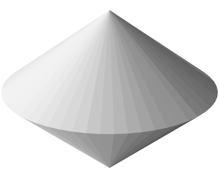
b Diamond shaped ${\mathcal{T}}_{D,k}$ for $k=50$.

Figure 4. Initial meshes for experiment in FEniCS, generated with tikzplotlib.

FEniCS [Aln+15] uses the Carey-Plaza algorithm [PC00] for mesh refinement, cf. Example 17 (c).

• We determine the mesh quantities for both initial meshes ${\mathcal{T}}_{F}$ and ${\mathcal{T}}_{D,50}$ experimentally for uniform mesh refinement. For uniform mesh refinement of the regular initial mesh ${\mathcal{T}}_{F}$ the Carey-Plaza algorithm coincides with the Freudenthal algorithm in Example 17 (a) and the bisection algorithms in Example 17 (b).

  Figure 5a displays the average quantity $\overline{e}$ plotted over the total number of vertices contained in the meshes. The experiment confirms the asymptotic behavior in the sense that $\overline{e}$ converges to $14$, as $V\to\infty$.

  

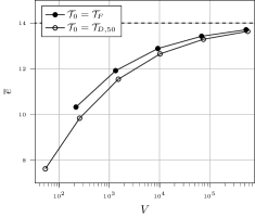
  a Uniform mesh refinement

  

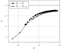
  b Adaptive mesh refinement

  Figure 5. Behavior of $\overline{e}$ for a family of meshes with $V$ vertices, generated by the Carey-Plaza algorithm from initial meshes ${\mathcal{T}}_{0}$.

• Additionally, we consider adaptive mesh refinement with the Carey-Plaza algorithm for both initial meshes. In each refinement step for the simplex containing the point $v^{*}\in\Omega\setminus\partial\Omega$ is refined, and the conforming closure is taken. As refinement point we choose $v^{*}=(\tfrac{1}{9},\tfrac{1}{3},\tfrac{1}{3})$, which is contained in both domains. Figure 5b shows the average quantities plotted over the total number of vertices contained in the meshes. In this case we cannot confirm convergence to $14$.

To the best of our knowledge there are no results on the asymptotic mesh quantities for adaptive mesh refinement schemes. This is left to future work.

4. Piecewise polynomials on split meshes

We now derive asymptotic formulæ for the dimensions of various finite element spaces on split 3D meshes in terms of the basic descriptors $\overline{e}$ and $V$ of the original mesh ${\mathcal{T}}$. This will allow us to compare the dimensions of the standard Scott–Vogelius elements on the original mesh ${\mathcal{T}}$ with elements using lower polynomial degrees on split meshes.

For a mesh $\widetilde{{\mathcal{T}}}$ and $k\geq 1$ we denote by $P_{k}(\widetilde{{\mathcal{T}}})$ the space of continuous, piecewise polynomial functions of polynomial degree at most $k$ on $\widetilde{{\mathcal{T}}}$. Then ${\bf V}_{k}(\widetilde{{\mathcal{T}}})$ denotes the space of vector-valued functions with each component in $P_{k}(\widetilde{{\mathcal{T}}})$, i.e., we have that $\dim({\bf V}_{k}(\widetilde{{\mathcal{T}}}))=3\dim(P_{k}(\widetilde{{\mathcal{T}}}))$. Furthermore, we denote by $\Pi_{k-1}(\widetilde{{\mathcal{T}}})$ the space of (discontinuous) piecewise polynomials of degree at most $k-1$ on $\widetilde{{\mathcal{T}}}$.

Let us first summarize the dimensions of the finite element spaces in terms of the mesh quantities $\widetilde{V},\widetilde{E},\widetilde{F}$ and $\widetilde{T}$, denoting the number of vertices, edges, faces and tetrahedra in $\widetilde{{\mathcal{T}}}$, respectively. Counting the Lagrange nodes we have

(16) $$\begin{split}\dim(P_{1}(\widetilde{{\mathcal{T}}}))&=\widetilde{V},\\ \dim(P_{2}(\widetilde{{\mathcal{T}}}))&=\widetilde{V}+\widetilde{E},\\ \dim(P_{k}(\widetilde{{\mathcal{T}}}))&=\widetilde{V}+(k-1)\widetilde{E}+\tfrac{1}{2}(k-1)(k-2)\widetilde{F}+\tfrac{1}{6}(k-1)(k-2)(k-3)\widetilde{T},\end{split}$$

for $k\geq 3$. Denoting by $P_{k-1}$ the space of polynomials of degree at most $k-1$ on a single tetrahedron, we also have

(17) $$\dim(\Pi_{k-1}(\widetilde{{\mathcal{T}}}))=\dim(P_{k-1})\widetilde{T}={2+k\choose k-1}\widetilde{T}\qquad\text{ for }k\geq 1.$$

Then, for the pressure space $\nabla\cdot{\bf V}_{k}(\widetilde{{\mathcal{T}}})\subset\Pi_{k-1}(\widetilde{{\mathcal{T}}})$ we obviously have

(18) $$\dim(\nabla\cdot{\bf V}_{k}(\widetilde{{\mathcal{T}}}))\leq\dim(\Pi_{k-1}(\widetilde{{\mathcal{T}}})).$$

Now we want to compute or estimate the dimensions of the mixed finite element spaces $({\bf V}_{k}(\widetilde{{\mathcal{T}}}),\nabla\cdot{\bf V}_{k}(\widetilde{{\mathcal{T}}}))$ on the original mesh ${\mathcal{T}}$ and the split meshes ${\mathcal{T}}_{{A}}$ and ${\mathcal{T}}_{{W}}$ as introduced in section 2, i.e., for $\widetilde{{\mathcal{T}}}\in\{{\mathcal{T}},{\mathcal{T}}_{{A}},{\mathcal{T}}_{{W}}\}$. For this we only need to combine the above identities (16), (17) and Lemma 2, which describes the mesh quantities of the split meshes in terms of the mesh quantities of the original mesh. Then we may apply the identities in Remark 5 to express the approximate dimensions in only $V$ and $\overline{e}$ for sufficiently large meshes. The resulting approximate dimensions in terms of $\overline{e}$ and $V$ are collected in Table 2, and for the case $\overline{e}=14$ they are collected in Table 3.

(r)[3pt]—c—c—c—c—c—c——cc—cc—c— mesh $\widetilde{{\mathcal{T}}}$ & ${\mathcal{T}}_{{W}}$ ${\mathcal{T}}_{{W}}$ ${\mathcal{T}}_{{A}}$ ${\mathcal{T}}$ ${\mathcal{T}}$
degree $k=1$ $k=2$ $k=3$ $k=4$ $k=6$
$\dim{\bf V}_{k}(\widetilde{{\mathcal{T}}})$ $(4.5\overline{e}-6)V$ $(27\overline{e}-48)V$ $(28.5\overline{e}-48)V$ $(15\overline{e}-18)V$ $(52.5\overline{e}-87)V$
$\dim{{\nabla\cdot}\,}{\bf V}_{k}(\widetilde{{\mathcal{T}}})$ $(4\overline{e}-8)V$ $(22\overline{e}-44)V$ $(20\overline{e}-40)V$ $(10\overline{e}-20)V$ $(28\overline{e}-56)V$
total $(8.5\overline{e}-14)V$ $(49\overline{e}-92)V$ $(48.5\overline{e}-88)V$ $(25\overline{e}-38)V$ $(80.5\overline{e}-143)V$

Table 2. Approximate dimensions of velocity space and approximate upper bound on the dimension of the pressure space. For an original mesh ${\mathcal{T}}$, the Worsey–Farin split ${\mathcal{T}}_{{W}}$ and the Alfeld split ${\mathcal{T}}_{{A}}$ are defined in section 4. The quantity $\overline{e}$ is defined in (5) and $V$ is the number of vertices in the original mesh ${\mathcal{T}}$. The approximate dimensions for the pressure space take into account the singular edges introduced by the split but do not take into account singular edges and vertices of ${\mathcal{T}}$.

(r)[3pt]—c—c—c—c—c—c——cc—cc—c— mesh $\widetilde{{\mathcal{T}}}$ & ${\mathcal{T}}_{{W}}$ ${\mathcal{T}}_{{W}}$ ${\mathcal{T}}_{{A}}$ ${\mathcal{T}}$ ${\mathcal{T}}$
degree   $k=1$      $k=2$       $k=3$      $k=4$      $k=6$   
$\dim{\bf V}_{k}(\widetilde{{\mathcal{T}}})$ $57V$ $330V$ $351V$ $162V$ $648V$
$\dim{{\nabla\cdot}\,}{\bf V}_{k}(\widetilde{{\mathcal{T}}})$ $48V$ $264V$ $240V$ $120V$ $336V$
total $105V$ $594$ $591V$ $282V$ $984V$

Table 3. Approximate dimensions of the velocity space and approximate upper bound on the dimension of the pressure space for $\overline{e}=14$.

One may have ${{\nabla\cdot}\,}{\bf V}_{k}(\widetilde{{\mathcal{T}}})\subsetneq\Pi_{k-1}(\widetilde{{\mathcal{T}}})$, and thus the dimension of the mixed finite element space $({\bf V}_{k}(\widetilde{{\mathcal{T}}}),\nabla\cdot{\bf V}_{k}(\widetilde{{\mathcal{T}}}))$ is slightly smaller than the one of $({\bf V}_{k}(\widetilde{{\mathcal{T}}}),\Pi_{k-1}(\widetilde{{\mathcal{T}}}))$. This is related to possible deficiencies in the mesh $\widetilde{{\mathcal{T}}}$ such as edge singularities.

In the following we shall neglect this effect for the original mesh ${\mathcal{T}}$, because in general there is no strategy to count or to characterize the pressure space available. However, we shall take into account the singular edges generated by the splits, since they are known and they have a substantial contribution.

4.1. Original mesh

Recall that the standard Scott–Vogelius element [SV85, SV85a] $({\bf V}_{k}({\mathcal{T}}),{{\nabla\cdot}\,}{\bf V}_{k}({\mathcal{T}}))$ is known to be inf-sup stable for $k\geq 6$ on the regular Freudenthal triangulation as in Example 7. This is proved in [Zha11]. Computational experiments on this mesh family [FMS22] suggest that the inf-sup condition holds for $k\geq 4$, independently of the mesh size $h$.

For this reason let us compute the approximate dimensions in both cases for general meshes for $({\bf V}_{k}({\mathcal{T}}),\Pi_{k-1}({\mathcal{T}}))$, i.e., neglecting singular edges. By (16), (17) for $k=6$ and $\widetilde{{\mathcal{T}}}={\mathcal{T}}$ and applying (6) we have

$$\dim{\bf V}_{6}({\mathcal{T}}) =3\dim P_{6}({\mathcal{T}})=3(V+5E+10F+10T)\approx(52.5\overline{e}-87)V,$$

$$\dim\Pi_{5}({\mathcal{T}}) =56T\approx(28\overline{e}-56)V,$$

compare the last column in Table 2. Using (16), (17) for $k=4$ and $\widetilde{{\mathcal{T}}}={\mathcal{T}}$ and (6) we have

$$\dim{\bf V}_{4}({\mathcal{T}}) =3\dim P_{4}({\mathcal{T}})=3(V+3E+3F+T)\approx(15\overline{e}-18)V,$$

$$\dim\Pi_{3}({\mathcal{T}}) =20T\approx(10\overline{e}-20)V,$$

compare the fifth column in Table 2.

4.2. Alfeld split

Alfeld splits subdivide tetrahedra into four subtetrahedra, see section 2. Given an initial mesh ${\mathcal{T}}$ we denote the resulting mesh by ${\mathcal{T}}_{{A}}$. It is known [Zha05] that the inf-sup condition is satisfied for the pair $({\bf V}_{k}({\mathcal{T}}_{{A}}),\Pi_{k-1}({\mathcal{T}}_{{A}}))$ for $k\geq 3$ in $d=3$ dimensions, see also [GN18, Nei20]. Indeed, for this split one has that $\Pi_{k-1}({\mathcal{T}}_{{A}})={{\nabla\cdot}\,}{\bf V}_{k}({\mathcal{T}}_{{A}})$. Let us compute the dimensions for the lowest order case $k=3$.

Using (16), (17) for $k=3$ and $\widetilde{{\mathcal{T}}}={\mathcal{T}}_{{A}}$, as well as Lemma 2 (i) and (6) we find that

$$\dim{\bf V}_{3}({\mathcal{T}}_{{A}}) =3\dim P_{3}({\mathcal{T}}_{{A}})=3(V_{A}+2E_{A}+F_{A})=3(V+2E+F+15T)$$

$$\approx(28.5\overline{e}-48)V,$$

$$\dim\Pi_{2}({\mathcal{T}}_{{A}}) =10T_{A}=40T\approx(20\overline{e}-40)V,$$

compare the fourth column in Table 2.

For the Scott–Vogelius elements [SV85, SV85a] on ${\mathcal{T}}$ for $k=4$ the pressure space has only half the size, cf. section 4.1. Note that a major contributor to the dimension is the large number of interior nodes of ${\bf V}_{3}({\mathcal{T}}_{{A}})$ compared to ${\bf V}_{4}({\mathcal{T}})$.

4.3. Worsey-Farin split

Worsey–Farin split subdivides tetrahedra into 12 subtetrahedra. Given an initial mesh ${\mathcal{T}}$, let ${\mathcal{T}}_{{W}}$ denote the resulting triangulation, cf. section 2. It is shown in [FGNZ22] that the inf-sup condition is satisfied for the pair $({\bf V}_{k}({\mathcal{T}}_{{W}}),{{\nabla\cdot}\,}{\bf V}_{k}({\mathcal{T}}_{{W}}))$ for $k\geq 1$ in $3$ dimensions. Therein for $k=1$ the pressure space ${{\nabla\cdot}\,}{\bf V}_{1}({\mathcal{T}}_{{W}})$ is characterized explicitly. See [Zha11a] for the case $k=2$.

Of course, ${{\nabla\cdot}\,}{\bf V}_{k}({\mathcal{T}}_{{W}})\subset\Pi_{k-1}({\mathcal{T}}_{{W}})$, but it can be a strict subspace [Zha11a], depending on the precise definition of the split. In [FGNZ22], the split is chosen so that on each face in ${\mathcal{T}}$, there are 3 singular edges (the dashed gray lines in Figure 1, right). A singular edge is an edge where exactly four faces meet, with opposite faces being coplanar. Thus there are 3 constraints per face [FGNZ22, Lemma 4.2].

Let us consider the lowest-order case $k=1$. Using (16) for $k=1$ and $\widetilde{{\mathcal{T}}}={\mathcal{T}}_{{W}}$, Lemma 2 (ii) and (6) we have

$$n_{V}\coloneqq\dim{\bf V}_{1}({\mathcal{T}}_{{W}}) =3\dim P_{1}({\mathcal{T}}_{{W}})=3V_{W}=3(V+F+T)$$

$$\approx(4.5\overline{e}-6)V,$$

compare the second column in Table 2. The space ${{\nabla\cdot}\,}{\bf V}_{1}({\mathcal{T}}_{{W}})$ is characterized in [FGNZ22, Prop. 6.1] and using (6) its dimension is bounded by

$$\dim{{\nabla\cdot}\,}{\bf V}_{1}({\mathcal{T}}_{{W}})\leq 4(F-F_{b})+F_{b}\approx 4(\overline{e}-2)V.$$

Note that this is smaller than

$$n_{\Pi}\coloneqq\dim\Pi_{0}({\mathcal{T}}_{{W}}) =T_{W}=12T\approx 6(\overline{e}-2)V,$$

see (17) for $k=1$ and $\widetilde{{\mathcal{T}}}={\mathcal{T}}_{{W}}$, Lemma 2 (ii) and (6). The functions in the larger space $\Pi_{0}({\mathcal{T}}_{{W}})$ but not in its subspace ${{\nabla\cdot}\,}{\bf V}_{1}({\mathcal{T}}_{{W}})$ are often referred to as missing modes. Although there are 3 constraints per face [FGNZ22, Lemma 4.2], only two of them are linearly independent. On the boundary, only one constraint is active. Thus the number of independent constraints is $2F-F_{b}=4T$, cf. (2). Indeed, asymptotically for large meshes, using (2) the number of missing modes is approximately

$$12T-4(F-F_{b})-F_{b}=12T-8T-2F_{b}+3F_{b}=4T+F_{b},$$

which is approximately $4T$ for sufficiently large meshes.

In the introduction of [FGNZ22] it is suggested that one could work with the constraints on the full variational space ${\bf V}_{1}({\mathcal{T}}_{{W}})\times\Pi_{0}({\mathcal{T}}_{{W}})$ of dimension $n_{V}+n_{\Pi}$ as defined above. This would require to use matrices of size $(n_{V}+n_{\Pi})\times(n_{V}+n_{\Pi})$. Note that the pressure space $\Pi_{0}({\mathcal{T}}_{{W}})$ is larger than the velocity space $n_{\Pi}>n_{V}$ for $\overline{e}>4$. In the Iterated Penalty Method (IPM) [BS08, Sco18], the matrices are of size $n_{V}\times n_{V}$, and they are symmetric and positive definite, so IPM may be competitive as indicated in [FGNZ22, Table 10]. Even if one would work directly with ${{\nabla\cdot}\,}{\bf V}_{1}({\mathcal{T}}_{{W}})$ as pressure space, which has dimension $\approx(4\overline{e}-8)V$, this is still comparable to $n_{V}$.

For the second order case, using (16), (17) for $k=2$ and $\widetilde{{\mathcal{T}}}={\mathcal{T}}_{{W}}$, as well as Lemma 2 (ii) and (6) we find that

(19) $$\dim{\bf V}_{2}({\mathcal{T}}_{{W}}) =3\dim P_{2}({\mathcal{T}}_{{W}})=3(V_{W}+E_{W})=3(V+E+4F+9T)$$

$$\approx(27\overline{e}-48)V,$$

$$\dim\Pi_{1}({\mathcal{T}}_{{W}}) =4T_{W}=48T\approx(24\overline{e}-48)V.$$

Again taking into account the singular edges, which yield the same number of constraints as in the lower-order case, we find that

(20) $$\dim{{\nabla\cdot}\,}{\bf V}_{2}({\mathcal{T}}_{{W}})\leq 48T-4T=44T\approx(22\overline{e}-44)V,$$

compare the third column in Table 2.

4.4. Compare and contrast

The lowest order case $k=1$ on the Worsey–Farin split mesh has by far the smallest dimension of the methods we compare. But for $k=2$, the dimension is larger than the one for the Scott–Vogelius element with $k=4$ on the original mesh, as indicated in Table 2 and 3. The same is true for $k=3$ on the Alfeld-split, for which the dimensions are very close to the case of quadratic velocity functions on ${\mathcal{T}}_{{W}}$. Indeed, for $\overline{e}\geq 4$ we find that

$$\dim{\bf V}_{3}({\mathcal{T}}_{{A}})\geq\dim{\bf V}_{2}({\mathcal{T}}_{{W}})+6V\geq\dim{\bf V}_{4}({\mathcal{T}})+24V.$$

However, the order of dimensions of the pressure spaces reverses:

$$\dim\Pi_{1}({\mathcal{T}}_{{W}})-4V\geq\dim{{\nabla\cdot}\,}{\bf V}_{2}({\mathcal{T}}_{{W}})\geq\dim\Pi_{2}({\mathcal{T}}_{{A}})+4V\geq\dim\Pi_{3}({\mathcal{T}})+24V,$$

for $\overline{e}\geq 4$.

For the value $\overline{e}=14$ we find that $({\bf V}_{2}({\mathcal{T}}_{{W}}),{{\nabla\cdot}\,}{\bf V}_{2}({\mathcal{T}}_{{W}}))$ and $({\bf V}_{3}({\mathcal{T}}_{{A}}),\Pi_{2}({\mathcal{T}}_{{A}}))$ have more than double the dimension of the Scott–Vogelius element for $k=4$, see Table 3. I.e., the size of the velocity and pressure spaces for $k=4$ on ${\mathcal{T}}$ are about half that of the low-order, inf-sup stable split methods for $k\geq 2$.

Furthermore, we can see that the size of the velocity and pressure spaces for $k=6$ on ${\mathcal{T}}$ are only about a factor of 4 larger than for $k=4$ on ${\mathcal{T}}$. Also the degree $k=6$ case is only about 50% bigger than the split methods for $k\geq 2$.

Remark 20 (2D case).

For comparison let us derive the corresponding dimensions of inf-sup stable piecewise polynomial finite element spaces in 2D. For a mesh $\widetilde{{\mathcal{T}}}$ in 2D we have that

(21) $$\dim(P_{1}(\widetilde{{\mathcal{T}}})) =\widetilde{V},$$

(22) $$\dim(P_{k}(\widetilde{{\mathcal{T}}})) =\widetilde{V}+(k-1)\widetilde{E}+\tfrac{1}{2}(k-1)(k-2)\widetilde{T}\quad\text{ for }k\geq 2,$$

and for $k\geq 1$ that

(23) $$\dim(\Pi_{k-1}(\widetilde{{\mathcal{T}}})) =\dim(P_{k-1}(\tau))\widetilde{T}={k+1\choose k-1}\widetilde{T}.$$

1. On the Alfeld split ${\mathcal{T}}_{{A}}$ the pair of spaces $({\bf V}_{k}({\mathcal{T}}_{{A}}),\Pi_{k-1}({\mathcal{T}}_{{A}}))$ are inf-sup stable for $k\geq 2$, see [AQ92, Qin94], see also [Nei20, Thm. 2.5]. For the case $k=2$ using Lemma 1 and Remark 3 we thus have

   $$\dim({\bf V}_{2}({\mathcal{T}}_{{A}})) =2(V_{A}+E_{A})=2(V+E+4T)$$

   $$=24V-10V_{b}-22\chi+10\chi_{b}\approx 24V,$$

   $$\dim(\Pi_{1}({\mathcal{T}}_{{A}})) =3T_{A}=9T=18V-9V_{b}-18\chi+9\chi_{b}\approx 18V,$$

   for meshes sufficiently large that we can neglect $V_{b},\chi$ and $\chi_{b}$.

2. On the Powell–Sabin split the space $({\bf V}_{1}({\mathcal{T}}_{{P}}),{{\nabla\cdot}\,}({\bf V}_{1}({\mathcal{T}}_{{P}})))$ is known to be inf-sup stable, see [Zha08]. The pressure space is contained in $\Pi_{0}({\mathcal{T}}_{{P}})$, but not fully characterized. Again by Lemma 1 and Remark 3 we thus have

   $$\dim({\bf V}_{1}({\mathcal{T}}_{{P}})) =2V_{P}=2(V+E+T)$$

   $$=12V-4V_{b}-10\chi+5\chi_{b}\approx 12V,$$

   $$\dim(\Pi_{0}({\mathcal{T}}_{{P}})) =T_{P}=6T=12V-6V_{b}-12\chi+6\chi_{b}\approx 12V,$$

   for meshes sufficiently large that we can neglect $V_{b},\chi$ and $\chi_{b}$. Taking into account the singular vertices on the edges for the Powell–Sabin split we find

   $$\dim({{\nabla\cdot}\,}{\bf V}_{1}({\mathcal{T}}_{{P}})) \leq 6T-E=9V-5V_{b}-9\chi-5\chi_{b}\approx 9V.$$

3. The Scott–Vogelius element on the original mesh ${\mathcal{T}}$ is inf-sup stable for $k\geq 4$, see [GS19]. For $k=4$ using Lemma 1 and Remark 3 we find

   $$\dim({\bf V}_{4}({\mathcal{T}})) =2(V+3E+3T)=32V-12V_{b}-30\chi\approx 32V,$$

   $$\dim(\Pi_{3}({\mathcal{T}})) =10T=20V-10V_{b}-20\chi+10\chi_{b}\approx 20V,$$

   for meshes sufficiently large that we can neglect $V_{b},\chi$ and $\chi_{b}$.

The bounds on the total approximate dimension of the pair of finite element spaces are $21V$ for the Sabin–Powell split and $k=1$, $42V$ for the Alfeld split and $k=2$, and $52V$ for the original mesh and $k=4$ (lowest order Scott–Vogelius element). The lowest order element on the Sabin–Powell has again the smallest dimension. Then, on the Alfeld split mesh the element of order $k=2$ follows with double the dimension. And finally, the Scott–Vogelius element with $k=4$ on the original mesh has only a slightly higher dimension.

5. Insights into the diagram

One application of the above counting strategy is to address the question of identifying the precursor space in a de Rham complex. By precursor space of a velocity space ${\bf V}_{k}({\mathcal{T}})\subset C(\overline{\Omega})$, we mean a subspace of ${\bf V}_{k+1}({\mathcal{T}})$, the curl of which coincides with the space of divergence-free functions in ${\bf V}_{k}({\mathcal{T}})$,

(24) $${\bf Z}_{k}({\mathcal{T}})\coloneqq\left\{{\bf v}\in{\bf V}_{k}({\mathcal{T}})\;:\;{{\nabla\cdot}\,}{\bf v}=0\right\}.$$

Thus, such a precursor space would be part of a discrete de Rham complex together with ${\bf V}_{k}({\mathcal{T}})$ and the pressure space ${{\nabla\cdot}\,}{\bf V}_{k}({\mathcal{T}})$.

In $d=2$ dimensions the identification of the full de Rham complex is relatively simple. The space ${\bf Z}_{k}({\mathcal{T}})$ of divergence-free continuous piecewise polynomial functions can be represented by the ${{\rm curl}\,}$ of all $C^{1}$ piecewise polynomials of degree $k+1$. This means, that the precursor space is the space of scalar functions $S_{k+1}({\mathcal{T}})\coloneqq P_{k+1}({\mathcal{T}})\cap C^{1}(\overline{\Omega})$, satisfying ${{\rm curl}\,}(S_{k+1}({\mathcal{T}}))={\bf Z}_{k}({\mathcal{T}})$. Often it is possible to identify the space of all $C^{1}$ piecewise polynomials. Indeed, for degree $k\geq 3$ a nodal basis is available [MS75, Sco19]. For some split mesh methods the same is true for lower polynomial degree. For example, on the Malkus split the Powell basis [Pow74] of $C^{1}$ piecewise quadratics is well known.

In $d=3$ dimensions the precursor space of ${\bf V}_{k}({\mathcal{T}})$ consists of vector-valued functions and shall be denoted by ${\bf\Upsilon}_{k+1}({\mathcal{T}})\subset{\bf V}_{k+1}({\mathcal{T}})$. By the assumption that ${\bf V}_{k}({\mathcal{T}})$ is conforming, the curl of functions in ${\bf\Upsilon}_{k+1}({\mathcal{T}})$ has to be continuous. But this does not necessarily require that ${\bf\Upsilon}_{k+1}({\mathcal{T}})\subset C^{1}(\overline{\Omega})$. Nevertheless, it is interesting to investigate spaces of $C^{1}$ piecewise polynomials on various split meshes, as split meshes were originally developed to construct such spaces. At the very least, their ${{\rm curl}\,}$ is a subspace of the divergence-free space. For this purpose we denote

(25) $${\bf S}_{r}({\mathcal{T}})\coloneqq{\bf V}_{r}({\mathcal{T}})\cap C^{1}(\overline{\Omega}),\quad\text{ for }r\in\mathbb{N}.$$

Since we have that ${{\rm curl}\,}{\bf S}_{k+1}({\mathcal{T}})\subset{\bf Z}_{k}({\mathcal{T}})=\{v\in{\bf V}_{k}({\mathcal{T}})\colon{{\nabla\cdot}\,}v=0\}$, it follows that ${\bf S}_{k+1}({\mathcal{T}})\subset{\bf\Upsilon}_{k+1}({\mathcal{T}})$.

For the generalized Powell–Sabin split as mentioned in section 2.2 above, each tetrahedron is split into $24$ tetrahedra. With ${\mathcal{T}}_{{P}}$ denoting the resulting mesh, the space ${\bf S}_{2}({\mathcal{T}}_{{P}})$ is studied in [WP88]. With the arguments above it is a candidate for a precursor space of ${\bf V}_{1}({\mathcal{T}}_{{P}})$. To the best of our knowledge nothing is known about the inf-sup stability of $({\bf V}_{1}({\mathcal{T}}_{{P}}),{{\nabla\cdot}\,}{\bf V}_{1}({\mathcal{T}}_{{P}}))$ in three dimensions.

On the Worsey–Farin split ${\mathcal{T}}_{{W}}$ as introduced in section 2.2 it is also not clear how to find a precursor space of ${\bf V}_{1}({\mathcal{T}}_{{W}})$. If we increase the degree to $k=2$, then the original Worsey–Farin paper [WF87] provides the space $S_{3}({\mathcal{T}}_{{W}})$. The vectorial version ${\bf S}_{3}({\mathcal{T}}_{{W}})$ serves as candidate for a precursor space of ${\bf V}_{2}({\mathcal{T}}_{{W}})$. For each component the degrees of freedom of ${\bf S}_{3}({\mathcal{T}}_{{W}})$ are 4 at each vertex and 2 on each edge, so with (6) we find

(26) $$\dim{\bf S}_{3}({\mathcal{T}}_{{W}})=3(4V+2E)\approx 3(\overline{e}+4)V,$$

for dimension $d=3$. Recalling the notation ${\bf Z}_{2}({\mathcal{T}}_{{W}})=\left\{v\in{\bf V}_{2}({\mathcal{T}}_{{W}})\;:\;{{\nabla\cdot}\,}v=0\right\}$, the gap between

$${{\rm curl}\,}{\bf S}_{3}({\mathcal{T}}_{{W}})\subset{\bf Z}_{2}({\mathcal{T}}_{{W}}),$$

can be significant, as the following theorem shows.

Theorem 21.

For a mesh ${\mathcal{T}}$ in 3D sufficiently large that we may neglect the boundary vertices and $\chi_{b},\chi$, cf. Remark 5, we consider its Worsey–Farin split ${\mathcal{T}}_{{W}}$ (cf. section 2.2). For $\overline{e}>8$, the space ${\bf Z}_{2}({\mathcal{T}}_{{W}})$ defined in (24) is strictly larger than the space ${{\rm curl}\,}{\bf S}_{3}({\mathcal{T}}_{{W}})$, with ${\bf S}_{3}({\mathcal{T}}_{{W}})$ as defined in (25). In particular, this is the case for large regular meshes as the Freudenthal triangulation, cf. Example 7 and for large meshes that arise from sufficiently many uniform mesh refinements, cf. Lemma 15.

Proof.

Applying (19) and (20) we obtain with (6) that

(27) $$\begin{split}\dim{\bf Z}_{2}({\mathcal{T}}_{{W}})&=\dim{\bf V}_{2}({\mathcal{T}}_{{W}})-\dim{{\nabla\cdot}\,}{\bf V}_{2}({\mathcal{T}}_{{W}})\geq 3(V+E+4F+9T)-44T\\ &\approx(27\overline{e}-48)V-(22\overline{e}-44)V=(5\overline{e}-4)V.\end{split}$$

From (26) it follows that

$$\dim{{\rm curl}\,}{\bf S}_{3}({\mathcal{T}}_{{W}})\leq\dim S_{3}({\mathcal{T}}_{{W}})=3(4V+2E)\approx 3(\overline{e}+4)V.$$

Combining both estimates we find that

(28) $$\begin{split}\dim{\bf Z}_{2}({\mathcal{T}}_{{W}})-\dim{{\rm curl}\,}{\bf S}_{3}({\mathcal{T}}_{{W}})&\geq 3V+3E+12F-17T-3(4V+2E)\\ &=-9V-3E+12F-17T\\ &\approx 2\big{(}\overline{e}-8\big{)}V.\end{split}$$

∎

For this reason the precursor space of ${\bf V}_{2}({\mathcal{T}}_{{W}})$ has to be larger than ${\bf S}_{3}({\mathcal{T}}_{{W}})$.

6. Conclusions and perspectives

We use a way of counting mesh quantities in three dimensions in terms of the average number of edges $\overline{e}$ meeting at a vertex. For $\overline{e}$ we presented upper and lower bounds. Furthermore, we reviewed asymptotic limits for a range of uniform mesh refinement schemes. These allowed us to compare the dimensions of various finite element spaces. We applied this to pairs of finite element spaces for problems with a divergence constraint, such as the incompressible Navier–Stokes equations. The mesh-counting techniques may be of independent interest in other contexts.

Although the use of split meshes lowers the degree for which finite element pairs with exact divergence constraints are stable, it may not yield smaller spaces. Indeed, only the lowest order example on the Worsey–Farin split has smaller dimension than the Scott–Vogelius element of polynomial degree $4$ on the original mesh. The fact that there is only one interior node per tetrahedron limits the size. The largest contributors are the face nodes, since they are nearly twice as plentiful as edge nodes. This means that when only considering the dimensions of the spaces, the most attractive higher order method is the Scott–Vogelius element for polynomial degree $k=4$.

Perhaps the main advantage of split meshes is that issues related to nearly singular vertices and edges are avoided. Still, the lower dimension of standard Scott–Vogelius methods of higher polynomial degree motivates to understand how to ameliorate nearly singular simplices in three dimensions.

7. Acknowledgments

We thank Patrick Farrell and Michael Neilan for valuable discussions and suggestions.

References

- [ABF84] D.. Arnold, F. Brezzi and M. Fortin “A stable finite element for the Stokes equations” In Calcolo 21.4, 1984, pp. 337–344 (1985) DOI: 10.1007/BF02576171
- [Aln+15] M. Alnæs et al. “The FEniCS Project Version 1.5” In Archiv of Numerical Software 3.100, 2015 DOI: 10.11588/ans.2015.100.20553
- [AQ92] D.. Arnold and J. Qin “Quadratic velocity/linear pressure Stokes elements” In Advances in computer methods for partial differential equations 7, 1992, pp. 28–34
- [AS05] P. Alfeld and L.. Schumaker “A trivariate macro-element based on the Clough-Tocher-split of a tetrahedron” In Comput. Aided Geom. Design 22.7, 2005, pp. 710–721 DOI: 10.1016/j.cagd.2005.06.007
- [Bän91] E. Bänsch “Local mesh refinement in and dimensions” In Impact Comput. Sci. Engrg. 3.3, 1991, pp. 181–191 DOI: 10.1016/0899-8248(91)90006-G
- [BBF13] D. Boffi, F. Brezzi and M. Fortin “Mixed Finite Element Methods and Applications” 44, Springer Series in Computational Mathematics Springer, Heidelberg, 2013, pp. xiv+685 DOI: 10.1007/978-3-642-36519-5
- [BDD04] P. Binev, W. Dahmen and R. DeVore “Adaptive finite element methods with convergence rates” In Numer. Math. 97.2, 2004, pp. 219–268 DOI: 10.1007/s00211-003-0492-7
- [Bey00] J. Bey “Simplicial grid refinement: on Freudenthal’s algorithm and the optimal number of congruence classes” In Numer. Math. 85.1, 2000, pp. 1–29 DOI: 10.1007/s002110050475
- [Bey95] J. Bey “Tetrahedral grid refinement” In Computing 55.4, 1995, pp. 355–378 DOI: 10.1007/BF02238487
- [BKK08] J. Brandts, S. Korotov and M. Křižek “On the equivalence of regularity criteria for triangular and tetrahedral finite element partitions” In Comput. Math. Appl. 55.10, 2008, pp. 2227–2233 DOI: 10.1016/j.camwa.2007.11.010
- [BR85] C. Bernardi and G. Raugel “Analysis of some finite elements for the Stokes problem” In Math. Comp. 44.169, 1985, pp. 71–79 DOI: 10.2307/2007793
- [BS08] Susanne C. Brenner and L. Scott “The mathematical theory of finite element methods” 15, Texts in Applied Mathematics Springer, New York, 2008, pp. xviii+397 DOI: 10.1007/978-0-387-75934-0
- [Cia02] P. Ciarlet “The Finite Element Method for Elliptic Problems” Reprint of the 1978 original [North-Holland, Amsterdam] 40, Classics in Applied Mathematics Society for IndustrialApplied Mathematics (SIAM), Philadelphia, PA, 2002, pp. xxviii+530 DOI: 10.1137/1.9780898719208
- [CR73] M. Crouzeix and P.-A. Raviart “Conforming and nonconforming finite element methods for solving the stationary Stokes equations I” In Rev. Française Automat. Informat. Recherche Opérationnelle Sér. Rouge 7.R-3, 1973, pp. 33–75 URL: http://eudml.org/doc/193250
- [Eul58] L. Euler “Elementa doctrinae solidorum” Nr. 230 In Euler Archive - All Works, 1758 URL: https://scholarlycommons.pacific.edu/euler-works/230
- [FGNZ22] M. Fabien, J. Guzmán, M. Neilan and A. Zytoon “Low-order divergence-free approximations for the Stokes problem on Worsey-Farin and Powell-Sabin splits” In Comput. Methods Appl. Mech. Engrg. 390, 2022, pp. Paper No. 114444\bibrangessep21 DOI: 10.1016/j.cma.2021.114444
- [FMS22] Patrick E. Farrell, Lawrence Mitchell and L. Scott “Two conjectures on the Stokes complex in three dimensions on Freudenthal meshes” arXiv, 2022 DOI: 10.48550/ARXIV.2211.05494
- [FMSW21] P.. Farrell, L. Mitchell, L.. Scott and F. Wechsung “A Reynolds-robust preconditioner for the Scott-Vogelius discretization of the stationary incompressible Navier-Stokes equations” In SMAI J. Comput. Math. 7, 2021, pp. 75–96 DOI: 10.5802/smai-jcm.72
- [FN13] R.. Falk and M. Neilan “Stokes complexes and the construction of stable finite elements with pointwise mass conservation” In SIAM J. Numer. Anal. 51.2, 2013, pp. 1308–1326 DOI: 10.1137/120888132
- [Fre42] H. Freudenthal “Simplizialzerlegungen von beschränkter Flachheit” In Ann. of Math. (2) 43, 1942, pp. 580–582 DOI: 10.2307/1968813
- [GLN20] J. Guzmán, A. Lischke and M. Neilan “Exact sequences on Powell-Sabin splits” In Calcolo 57.2, 2020, pp. Paper No. 13\bibrangessep25 DOI: 10.1007/s10092-020-00361-x
- [GN14] J. Guzmán and M. Neilan “Conforming and divergence-free Stokes elements in three dimensions” In IMA Journal of Numerical Analysis 34.4, 2014, pp. 1489–1508 DOI: 10.1093/imanum/drt053
- [GN14a] J. Guzmán and M. Neilan “Conforming and divergence-free Stokes elements on general triangular meshes” In Math. Comp. 83, 2014, pp. 15–36
- [GN18] J. Guzmán and M. Neilan “Inf-sup stable finite elements on barycentric refinements producing divergence-free approximations in arbitrary dimensions” In SIAM Journal on Numerical Analysis 56.5 SIAM, 2018, pp. 2826–2844
- [GS19] J. Guzmán and L.. Scott “The Scott-Vogelius finite elements revisited” In Math. Comp. 88.316, 2019, pp. 515–529 DOI: 10.1090/mcom/3346
- [Hat02] A. Hatcher “Algebraic topology” Cambridge University Press, Cambridge, 2002, pp. xii +544
- [JLMNR17] V. John, A. Linke, C. Merdon, M. Neilan and L.. Rebholz “On the divergence constraint in mixed finite element methods for incompressible flows” In SIAM Rev. 59.3, 2017, pp. 492–544 DOI: 10.1137/15M1047696
- [Kos94] I. Kossaczký “A recursive approach to local mesh refinement in two and three dimensions” In J. Comput. Appl. Math. 55.3, 1994, pp. 275–288 DOI: 10.1016/0377-0427(94)90034-5
- [Kuh60] H.. Kuhn “Some combinatorial lemmas in topology” In IBM J. Res. Develop. 4, 1960, pp. 508–524 DOI: 10.1147/rd.45.0518
- [LJ95] A. Liu and B. Joe “Quality local refinement of tetrahedral meshes based on bisection” In SIAM J. Sci. Comput. 16.6, 1995, pp. 1269–1291 DOI: 10.1137/0916074
- [Mat19] The MathWorks, Inc. “Symbolic Math Toolbox”, 2019 URL: https://www.mathworks.com/help/symbolic/
- [Mau94] J… Maubach “Iterative methods for non-linear partial differential equations” 92, CWI Tract Stichting Mathematisch Centrum, Centrum voor Wiskunde en Informatica, Amsterdam, 1994, pp. xiv+24
- [Mau95] J.. Maubach “Local bisection refinement for -simplicial grids generated by reflection” In SIAM J. Sci. Comput. 16.1, 1995, pp. 210–227 DOI: 10.1137/0916014
- [MH78] D.. Malkus and T..R. Hughes “Mixed finite element methods — Reduced and selective integration techniques: A unification of concepts” In Computer Methods in Applied Mechanics and Engineering 15.1, 1978, pp. 63–81 DOI: https://doi.org/10.1016/0045-7825(78)90005-1
- [Mit91] W.. Mitchell “Adaptive refinement for arbitrary finite-element spaces with hierarchical bases” In J. Comput. Appl. Math. 36.1, 1991, pp. 65–78 DOI: 10.1016/0377-0427(91)90226-A
- [MO84] D.. Malkus and E.. Olsen “Linear crossed triangles for incompressible media” In Unification of finite element methods 94, North-Holland Math. Stud. North-Holland, Amsterdam, 1984, pp. 235–248 DOI: 10.1016/S0304-0208(08)72627-6
- [MS75] J. Morgan and R. Scott “A nodal basis for piecewise polynomials of degree ” In Math. Comput. 29, 1975, pp. 736–740 DOI: 10.2307/2005284
- [MW95] D Moore and J Warren “Adaptive simplicial mesh quadtrees” In Houston J. Math 21.3, 1995, pp. 525–540
- [Nei20] M. Neilan “The Stokes complex: a review of exactly divergence-free finite element pairs for incompressible flows” In 75 years of mathematics of computation 754, Contemp. Math. Amer. Math. Soc., [Providence], RI, 2020, pp. 141–158 DOI: 10.1090/conm/754/15142
- [PC00] A. Plaza and G.. Carey “Local refinement of simplicial grids based on the skeleton” In Appl. Numer. Math. 32.2, 2000, pp. 195–218 DOI: 10.1016/S0168-9274(99)00022-7
- [Pow74] M. J.. Powell “Piecewise quadratic surface fitting for contour plotting” In Software for numerical mathematics (Proc. Conf., Inst. Math. Appl., Loughborough Univ. Tech., Loughborough, 1973), 1974, pp. 253–271
- [PR02] A. Plaza and M.-C. Rivara “On the adjacencies of triangular meshes based on skeleton-regular partitions” In Proceedings of the 9th International Congress on Computational and Applied Mathematics (Leuven, 2000) 140 (1-2), 2002, pp. 673–693 DOI: 10.1016/S0377-0427(01)00484-8
- [PR03] A. Plaza and M.-C. Rivara “Mesh Refinement Based on the 8-Tetrahedra Longest-Edge Partition” In Proceedings of the 12th International Meshing Roundtable, IMR 2003, Santa Fe, New Mexico, USA, September 14-17, 2003, 2003, pp. 67–78 URL: http://imr.sandia.gov/papers/abstracts/Pl292.html
- [PR05] A. Plaza and M.. Rivara “Average adjacencies for tetrahedral skeleton-regular partitions” In J. Comput. Appl. Math. 177.1, 2005, pp. 141–158 DOI: 10.1016/j.cam.2004.09.013
- [PS77] M… Powell and M.. Sabin “Piecewise quadratic approximations on triangles” In ACM Trans. Math. Software 3.4, 1977, pp. 316–325 DOI: 10.1145/355759.355761
- [Qin94] J. Qin “On the convergence of some low order mixed finite elements for incompressible fluids” Thesis (Ph.D.)–The Pennsylvania State University ProQuest LLC, Ann Arbor, MI, 1994, pp. 158 URL: http://gateway.proquest.com/openurl?url_ver=Z39.88-2004&rft_val_fmt=info:ofi/fmt:kev:mtx:dissertation&res_dat=xri:pqdiss&rft_dat=xri:pqdiss:9504277
- [Riv84] M.-C. Rivara “Algorithms for refining triangular grids suitable for adaptive and multigrid techniques” In Internat. J. Numer. Methods Engrg. 20.4, 1984, pp. 745–756 DOI: 10.1002/nme.1620200412
- [Riv91] M.-C. Rivara “Local modification of meshes for adaptive and/or multigrid finite-element methods” In J. Comput. Appl. Math. 36.1, 1991, pp. 79–89 DOI: 10.1016/0377-0427(91)90227-B
- [Sco18] L.. Scott “Introduction to Automated Modeling with FEniCS” Computational Modeling Initiative LLC, 2018
- [Sco19] L. Scott “ Piecewise Polynomials Satisfying Boundary Conditions”, 2019
- [Spe28] E. Sperner “Ein Satz über Untermengen einer endlichen Menge” In Math. Z. 27.1, 1928, pp. 544–548 DOI: 10.1007/BF01171114
- [Sta92] R.. Stanley “Subdivisions and local -vectors” In J. Amer. Math. Soc. 5.4, 1992, pp. 805–851 DOI: 10.2307/2152711
- [Ste08] R. Stevenson “The completion of locally refined simplicial partitions created by bisection” In Math. Comp. 77.261, 2008, pp. 227–241 DOI: 10.1090/S0025-5718-07-01959-X
- [SV85] L.. Scott and M. Vogelius “Conforming finite element methods for incompressible and nearly incompressible continua” In Large-scale computations in fluid mechanics, Part 2 (La Jolla, Calif., 1983) 22, Lectures in Appl. Math. Amer. Math. Soc., Providence, RI, 1985, pp. 221–244 DOI: 10.1051/m2an/1985190101111
- [SV85a] L.. Scott and M. Vogelius “Norm estimates for a maximal right inverse of the divergence operator in spaces of piecewise polynomials” In (formerly R.A.I.R.O. Analyse Numérique) 19.1, 1985, pp. 111–143 DOI: 10.1051/m2an/1985190101111
- [SW19] N. Salepci and J.-Y. Welschinger “Asymptotic measures and links in simplicial complexes” In Discrete Comput. Geom. 62.1, 2019, pp. 164–179 DOI: 10.1007/s00454-019-00091-0
- [TH73] C. Taylor and P. Hood “A numerical solution of the Navier-Stokes equations using the finite element technique” In Internat. J. Comput. & Fluids 1, 1973, pp. 73–100 DOI: 10.1016/0045-7930(73)90027-3
- [Tra97] C.. Traxler “An algorithm for adaptive mesh refinement in dimensions” In Computing 59.2, 1997, pp. 115–137 DOI: 10.1007/BF02684475
- [Wes96] D.. West “Introduction to graph theory” Prentice Hall, Inc., Upper Saddle River, NJ, 1996, pp. xvi+512
- [WF87] A.. Worsey and G. Farin “An -dimensional Clough-Tocher interpolant” In Constr. Approx. 3.2 Springer, 1987, pp. 99–110 DOI: 10.1007/BF01890556
- [WP88] A.. Worsey and B. Piper “A trivariate Powell–Sabin interpolant” In Comput. Aided Geom. Design 5.3 Elsevier, 1988, pp. 177–186 DOI: 10.1016/0167-8396(88)90001-5
- [Zha05] S. Zhang “A new family of stable mixed finite elements for the 3D Stokes equations” In Math. Comp. 74.250, 2005, pp. 543–554 DOI: 10.1090/S0025-5718-04-01711-9
- [Zha08] S. Zhang “On the P1 Powell-Sabin divergence-free finite element for the Stokes equations” In J. Comput. Math. 26.3, 2008, pp. 456–470
- [Zha11] S. Zhang “Divergence-free finite elements on tetrahedral grids for ” In Math. Comp. 80.274, 2011, pp. 669–695 DOI: 10.1090/S0025-5718-2010-02412-3
- [Zha11a] S. Zhang “Quadratic divergence-free finite elements on Powell–Sabin tetrahedral grids” In Calcolo 48.3 Springer, 2011, pp. 211–244 DOI: 10.1007/s10092-010-0035-4
- [Zha95] S. Zhang “Successive subdivisions of tetrahedra and multigrid methods on tetrahedral meshes” In Houston J. Math. 21.3, 1995, pp. 541–556
- [Zie95] G.. Ziegler “Lectures on polytopes” 152, Graduate Texts in Mathematics Springer-Verlag, New York, 1995, pp. x+370 DOI: 10.1007/978-1-4613-8431-1