Randomized Kaczmarz method with adaptive stepsizes for inconsistent linear systems

Abstract.

We investigate the randomized Kaczmarz method that adaptively updates the stepsize using readily available information for solving inconsistent linear systems. A novel geometric interpretation is provided which shows that the proposed method can be viewed as an orthogonal projection method in some sense. We prove that this method converges linearly in expectation to the unique minimum Euclidean norm least-squares solution of the linear system, and provide a tight upper bound for the convergence of the proposed method. Numerical experiments are also given to illustrate the theoretical results.

1. Introduction

Solving systems of linear equations is a fundamental problem in scientific computing and engineering. It comes up in many real-world applications such as signal processing [6], optimal control [41], machine learning [8], and partial differential equations [40]. The Kaczmarz method [24], also known as algebraic reconstruction technique (ART) [22, 15], is a classic yet effective row-action iteration solver for solving the large-scale linear system of equations

(1) $$Ax=b,\ A\in\mathbb{R}^{m\times n},\ b\in\mathbb{R}^{m}.$$

At each step of the original Kaczmarz method, a row of the system is sampled and the previous iterate is orthogonally projected onto the hyperplane defined by that row.

In the literature, there are empirical evidences that using the rows of the matrix $A$ in a random order rather than a deterministic order can often accelerate the convergence of the Kaczmarz method [22, 32, 13]. In the seminal paper [47], Strohmer and Vershynin studied the randomized Kaczmarz (RK) method and proved its linear convergence in expectation provided that the linear system (1) is consistent. Subsequently, there is a large amount of work on the development of the Kaczmarz-type methods including accelerated randomized Kaczmarz methods [27, 19, 28], block Kaczmarz methods [33, 36, 31, 17], greedy randomized Kaczmarz methods [2, 16], randomized sparse Kaczmarz methods [45, 9], etc. Nevertheless, all of these methods will not converge if the linear system (1) is not consistent. Indeed, Needell [34] showed that RK applied to inconsistent linear systems converges only to within a radius (convergence horizon) of the least-squares solution (see Theorem 2.1); see also [4] for some further comments.

It is well-known that the so-called relaxation parameters or stepsizes $\lambda_{1},\ldots,\lambda_{k}$ are important for the Kaczmarz method in practice. The original Kaczmarz method with decreasing stepsizes for solving inconsistent systems has been investigated in [7, 20]. It has been shown that with the stepsizes being nearly zero and appropriate initial point, the Kaczmarz method converges inside the convergence horizon to the minimum Euclidean norm least-squares solution. However, its convergence rate is difficult to obtain. Hence, for the RK method, a natural and interesting question is that is it possible that with carefully designed stepsizes the RK method is convergent for solving inconsistent systems? Furthermore, can the convergence rate of the proposed method be obtained easily?

Actually, the randomized extended Kaczmarz (REK) method [51, 10] has already provided a positive answer to the above questions. Section 3.3 will provide more detailed comments on this topic. Furthermore, there is enormous of work on the developments and extensions of the REK method, including the block or deterministic variants of REK [49, 37, 12, 11, 50, 48, 42, 43, 3], greedy randomized augmented Kaczmarz (GRAK) method [4], randomized extended Gauss-Seidel (REGS) method [10, 30], etc. We note that those methods make use of both rows and columns of $A$ at each step (see (10)) and work for general linear systems (consistent or inconsistent, full-rank or rank-deficient). Another randomized method that can be used to solve inconsistent systems with full column-rank coefficient matrix is the randomized coordinate descent (RCD) method [26], we refer to [1] for more discussions about the RCD method.

In this paper, we further investigate the RK method with adaptive stepsizes for solving inconsistent systems and provide an alternative strategy to answer the above questions. Our proposed geometric interpretation demonstrates that the method can be viewed as an orthogonal projection method in some sense. By utilizing this interpretation, we show that our strategy is effective in simplifying the analysis and endows the proposed method with a linear convergence rate. Additionally, we conduct a comprehensive comparison between the proposed method and the REK method, including their geometric interpretation, theoretical analysis, and numerical behavior.

The remainder of the paper is organized as follows. After introducing some preliminaries in Section 2, we present and analyze the RK method with adaptive stepsizes in Section 3. In Section 4, we perform some numerical experiments to show the effectiveness of the proposed method. Finally, we conclude the paper in Section 5.

2. Preliminaries

2.1. Notations

Throughout the paper, for any random variables $\xi$ and $\zeta$, we use $\mathbb{E}[\xi]$ and $\mathbb{E}[\xi\lvert\zeta]$ to denote the expectation of $\xi$ and the conditional expectation of $\xi$ given $\zeta$. For an integer $m\geq 1$, let $[m]:=\{1,\ldots,m\}$. Given $T\subset[m]$, the cardinality of the set $T$ is denoted by $\mid T\mid$. For any vector $x\in\mathbb{R}^{n}$, we use $x_{i},x^{\top}$, and $\|x\|_{2}$ to denote the $i$-th entry, the transpose and the Euclidean norm of $x$, respectively. For any matrix $A\in\mathbb{R}^{m\times n}$, we use $A_{i,:},A_{:,j},A^{\top},A^{\dagger},\|A\|_{2},\|A\|_{F}$, $\mbox{Range}(A)$, and $\text{Null}(A)$ to denote the $i$-th row, the $j$-th column, the transpose, the Moore-Penrose pseudoinverse, the spectral norm, the Frobenius norm, the column space, and the null space of $A$, respectively. For any $x,y\in\mathbb{R}^{n}$, the Hadamard product of $x$ and $y$ is defined to be the entrywise product $(x\circ y)_{i}=x_{i}y_{i}$. The nonzero singular values of a matrix $A$ are $\sigma_{1}(A)\geq\sigma_{2}(A)\geq\ldots\geq\sigma_{r}(A):=\sigma_{\min}(A)>0$, where $r$ is the rank of $A$ and $\sigma_{\min}(A)$ denotes the smallest nonzero singular values of $A$. We see that $\|A\|_{2}=\sigma_{1}(A)$ and $\|A\|_{F}=\sqrt{\sum\limits_{i=1}^{r}\sigma_{i}(A)^{2}}$.

2.2. The pseudoinverse solution

In this paper, we are interested in the pseudoinverse solution $A^{\dagger}b$ of the linear system (1). Here we would like to make clear what $A^{\dagger}b$ represents in different cases of linear systems [14, 5, 11]. Table 1 summarizes the results.

Table 1. The pseudoinverse solution $A^{\dagger}b$ of $Ax=b$.

$Ax=b$	$\operatorname{rank}(A)$	$A^{\dagger}b$
consistent	$=n$	unique solution
consistent	$<n$	unique minimum Euclidean norm solution
inconsistent	$=n$	unique least-squares (LS) solution
inconsistent	$<n$	unique minimum Euclidean norm LS solution

2.3. The RK method

The RK method for solving the linear system (1) begins with an arbitrary vector $x^{0}$, and in the $k$-th iteration iterates by

(2) $$x^{k+1}=x^{k}-\lambda\frac{A_{i_{k},:}x^{k}-b_{i_{k}}}{\|A_{i_{k},:}\|^{2}_{2}}A_{i_{k},:}^{\top},$$

where the index $i_{k}$ is i.i.d. selected from $[m]$ and $\lambda\in(0,2)$ is the stepsize. When $\lambda=1$, it reduces to the classical RK method. In the seminal paper [47], Strohmer and Vershynin proved the first linear convergence rate of the RK method for consistent systems. Later, Needell [34, 35] studied the RK method for inconsistent cases. The result is precisely restated below.

Theorem 2.1 ([35], Corollary 5.1).

Starting from any initial vector $x^{0}\in\text{Range}(A^{\top})$, the expected error of the RK method (2) in the $k$-th iteration satisfies

(3) $$\mathbb{E}\left[\left\|x^{k}-A^{\dagger}b\right\|^{2}_{2}\right]\leq\left(1-2\lambda(1-\lambda)\frac{\sigma^{2}_{\min}(A)}{\|A\|^{2}_{F}}\right)^{k}\left\|x^{0}-A^{\dagger}b\right\|^{2}_{2}+\frac{\lambda a^{2}_{\max}\|e\|^{2}_{2}}{(1-\lambda)a^{2}_{\min}\sigma^{2}_{\min}(A)},$$

where the index $i$ is selected with probability $\frac{\|A_{i,:}\|^{2}_{2}}{\|A\|^{2}_{F}}$, $\lambda\in(0,1)$, $e=AA^{\dagger}b-b$, $a^{2}_{\min}=\min\limits_{i\in[m]}\|A_{i,:}\|^{2}_{2}$, and $a^{2}_{\max}=\max\limits_{i\in[m]}\|A_{i,:}\|^{2}_{2}$.

It can be seen that for arbitrary $\lambda$, the above result implies a tradeoff between a smaller convergence horizon and a slower convergence. In this paper, we study the RK method with adaptive stepsizes $\lambda_{k}$ to eliminate the last term in (3) (see Corollary 3.2).

3. Adaptive stepsizes for RK

In this section, we introduce RK with adaptive stepsizes (RKAS) for solving the linear system (1). The method is formally described in Algorithm 1.

Algorithm 1 RK with adaptive stepsizes (RKAS)

$A\in\mathbb{R}^{m\times n}$, $b\in\mathbb{R}^{m}$, $k=0$ and initial points $x^{0}=0,r^{0}=Ax^{0}-b=-b$.

1. Select $i_{k}\in[m]$ with probability $\mbox{Pr}(i_{k}=i)=\frac{\|A_{i,:}\|^{2}_{2}}{\|A\|_{F}^{2}}$.

2. Compute

   $$\alpha_{k}=\frac{\langle AA_{i_{k},:}^{\top},r^{k}\rangle}{\|AA_{i_{k},:}^{\top}\|^{2}_{2}}.$$

3. Update

   $$x^{k+1} =x^{k}-\alpha_{k}A_{i_{k},:}^{\top},$$

   $$r^{k+1} =r^{k}-\alpha_{k}AA_{i_{k},:}^{\top}.$$

4. If the stopping rule is satisfied, stop and go to output. Otherwise, set $k=k+1$ and return to Step $1$.

The approximate solution.

Note that the most expensive computational cost in the $k$-th iteration of Algorithm 1 is to compute $AA_{i_{k},:}^{\top}$. Let $B:=AA^{\top}$, then $B_{:,i_{k}}=AA_{i_{k},:}^{\top}$. Thus, if it is possible to store $B=AA^{\top}$ at the initialization, Algorithm 1 could be faster in practice. In fact, this strategy is also adopted by the greedy randomized Kaczmarz method [4, 2] and the weighted randomized Kaczmarz method [46].

3.1. A geometric interpretation

We present an intuitive geometric explanation of Algorithm 1 in this subsection. Consider the following least-squares problem

$$\min\limits_{x\in\mathbb{R}^{n}}f(x):=\frac{1}{2}\|Ax-b\|^{2}_{2}.$$

Since

$$f(x) =\frac{1}{2}x^{\top}A^{\top}Ax-x^{\top}A^{\top}b+\frac{1}{2}\|b\|_{2}^{2}$$

$$=\frac{1}{2}x^{\top}A^{\top}Ax-x^{\top}A^{\top}AA^{\dagger}b+\frac{1}{2}\|b\|_{2}^{2}$$

$$=\frac{1}{2}\|Ax-AA^{\dagger}b\|^{2}_{2}-\frac{1}{2}\|AA^{\dagger}b\|^{2}_{2}+\frac{1}{2}\|b\|_{2}^{2},$$

where the second equality follows from the fact that $A^{\top}AA^{\dagger}b=A^{\top}b$. This implies that the least-squares problem can be equivalently reformulated as

(4) $$\min\limits_{x\in\mathbb{R}^{n}}\frac{1}{2}\|Ax-AA^{\dagger}b\|^{2}_{2}.$$

When using RK (2) to solve the least-squares problem (4), in the $k$-th iteration, we may expect the distance between $Ax^{k+1}$ and $AA^{\dagger}b$ to be as small as possible. This leads to the following optimization problem:

(5) $${\boxed{x^{k+1}=\arg\min\limits_{x\in\mathbb{R}^{n}}\|Ax-AA^{\dagger}b\|^{2}_{2}\ \ \text{subject to}\ \ x=x^{k}-\lambda\frac{A_{i_{k},:}x^{k}-b_{i_{k}}}{\|A_{i_{k},:}\|^{2}_{2}}A_{i_{k},:}^{\top},\ \lambda\in\mathbb{R}.}}$$

Note that $r^{k+1}$ in Step $3$ is actually obtained by an incremental method

$$r^{k+1}=r^{k}-\alpha_{k}AA_{i_{k},:}^{\top}=Ax^{k}-b-\alpha_{k}AA_{i_{k},:}^{\top}=Ax^{k+1}-b.$$

Using the fact that $A^{\top}AA^{\dagger}b=A^{\top}b$ and letting $\gamma_{k}=\frac{A_{i_{k},:}x^{k}-b_{i_{k}}}{\|A_{i_{k},:}\|^{2}_{2}}$, then the minimizer of (5) is achieved when

$$\lambda_{k}^{*}=\frac{\langle AA_{i_{k},:}^{\top},Ax^{k}-AA^{\dagger}b\rangle}{\|AA_{i_{k},:}^{\top}\|^{2}_{2}\gamma_{k}}=\frac{\langle AA_{i_{k},:}^{\top},Ax^{k}-b\rangle}{\|AA_{i_{k},:}^{\top}\|^{2}_{2}\gamma_{k}}=\frac{\langle AA_{i_{k},:}^{\top},r^{k}\rangle}{\|AA_{i_{k},:}^{\top}\|^{2}_{2}\gamma_{k}}.$$

Hence

$$x^{k+1}=x^{k}-\lambda^{*}_{k}\gamma_{k}A_{i_{k},:}=x^{k}-\frac{\langle AA_{i_{k},:}^{\top},r^{k}\rangle}{\|AA_{i_{k},:}^{\top}\|^{2}_{2}}A_{i_{k},:}^{\top}=x^{k}-\alpha_{k}A_{i_{k},:}^{\top},$$

which is exactly the iteration in Step 3 of Algorithm 1. It follows from (5) that $x^{k+1}$ obtained by Algorithm 1 satisfies that $Ax^{k+1}$ is the orthogonal projection of $AA^{\dagger}b$ onto $Ax^{k}+\text{Span}\{AA_{i_{k},:}^{\top}\}$. The geometric interpretation of Algorithm 1 is presented in Figure 1.

Figure 1. A geometric interpretation of Algorithm 1. The next iterate $x^{k+1}$ arises such that $Ax^{k+1}$ is the projection of $AA^{\dagger}b$ onto $Ax^{k}+\mbox{Span}\{AA_{i_{k},:}^{\top}\}$.

3.2. Convergence analysis

We now state our convergence results. The following result is about the convergence for $\mathbb{E}[\|Ax^{k}-AA^{\dagger}b\|^{2}_{2}]$.

Theorem 3.1.

For any given linear system $Ax=b$, let $\{x^{k}\}_{k=0}^{\infty}$ be the iteration sequence generated by Algorithm 1 with $x^{0}=0$. Then

$$\mathbb{E}\left[\left\|Ax^{k}-AA^{\dagger}b\right\|^{2}_{2}\right]\leq\left(1-\frac{\sigma_{\min}^{4}(A)}{\|A\|_{2}^{2}\|A\|_{F}^{2}}\right)^{k}\left\|Ax^{0}-AA^{\dagger}b\right\|^{2}_{2}.$$

Proof.

Since $Ax^{k+1}-AA^{\dagger}b$ and $AA_{i_{k},:}^{\top}$ are orthogonal, we have

$$\left\|Ax^{k+1}-AA^{\dagger}b\right\|^{2}_{2} =\left\|Ax^{k}-AA^{\dagger}b\right\|^{2}_{2}-\left\|Ax^{k+1}-Ax^{k}\right\|^{2}_{2}$$

$$=\left\|Ax^{k}-AA^{\dagger}b\right\|^{2}_{2}-\frac{\langle AA_{i_{k},:}^{\top},r^{k}\rangle^{2}}{\|AA_{i_{k},:}^{\top}\|^{2}_{2}}$$

$$=\left\|Ax^{k}-AA^{\dagger}b\right\|^{2}_{2}-\frac{\langle AA_{i_{k},:}^{\top},Ax^{k}-b\rangle^{2}}{\|AA_{i_{k},:}^{\top}\|^{2}_{2}}$$

$$=\left\|Ax^{k}-AA^{\dagger}b\right\|^{2}_{2}-\frac{\langle AA_{i_{k},:}^{\top},Ax^{k}-AA^{\dagger}b\rangle^{2}}{\|AA_{i_{k},:}^{\top}\|^{2}_{2}},$$

where the last equality follows from $A^{\top}b=A^{\top}AA^{\dagger}b$. Hence

(6) $$\mathbb{E}\left[\left\|Ax^{k+1}-AA^{\dagger}b\right\|^{2}_{2}\bigg{|}x^{k}\right] =\left\|Ax^{k}-AA^{\dagger}b\right\|^{2}_{2}-\sum\limits_{i=1}^{m}\frac{\|A_{i,:}\|^{2}_{2}}{\|A\|^{2}_{F}}\frac{\langle AA_{i,:}^{\top},Ax_{k}-AA^{\dagger}b\rangle^{2}}{\|AA_{i,:}^{\top}\|^{2}_{2}}$$

$$\leq\left\|Ax^{k}-AA^{\dagger}b\right\|^{2}_{2}-\sum\limits_{i=1}^{m}\frac{\|A_{i,:}\|^{2}_{2}}{\|A\|^{2}_{F}}\frac{\langle AA_{i,:}^{\top},Ax^{k}-AA^{\dagger}b\rangle^{2}}{\|A\|^{2}_{2}\|A_{i,:}\|^{2}_{2}}$$

$$=\left\|Ax^{k}-AA^{\dagger}b\right\|^{2}_{2}-\sum\limits_{i=1}^{m}\frac{\langle AA_{i,:}^{\top},Ax^{k}-AA^{\dagger}b\rangle^{2}}{\|A\|^{2}_{2}\|A\|^{2}_{F}}$$

$$=\left\|Ax^{k}-AA^{\dagger}b\right\|^{2}_{2}-\frac{\|AA^{\top}(Ax^{k}-AA^{\dagger}b)\|_{2}^{2}}{\|A\|^{2}_{2}\|A\|^{2}_{F}}$$

$$\leq\left(1-\frac{\sigma^{4}_{\min}(A)}{\|A\|_{2}^{2}\|A\|^{2}_{F}}\right)\left\|Ax^{k}-AA^{\dagger}b\right\|^{2}_{2},$$

where the first inequality follows from $\|AA_{i,:}^{\top}\|_{2}\leq\|A\|_{2}\|A_{i,:}\|_{2}$ and the last inequality follows from the fact that $A(x^{k}-A^{\dagger}b)\in\text{Range}(AA^{\top})$. Taking expectation over the entire history we have

$$\mathbb{E}\left[\left\|Ax^{k+1}-AA^{\dagger}b\right\|^{2}_{2}\right]\leq\left(1-\frac{\sigma^{4}_{\min}(A)}{\|A\|_{2}^{2}\|A\|^{2}_{F}}\right)\mathbb{E}\left[\left\|Ax^{k}-AA^{\dagger}b\right\|^{2}_{2}\right].$$

By induction on the iteration index $k$, we can obtain the desired result. ∎

By Theorem 3.1, we can obtain the following linear convergence for the expected norm of the error.

Corollary 3.2.

For any given linear system $Ax=b$, let $\{x^{k}\}_{k=0}^{\infty}$ be the iteration sequence generated by Algorithm 1 with $x^{0}=0$. Then

$$\mathbb{E}\left[\left\|x^{k}-A^{\dagger}b\right\|^{2}_{2}\right]\leq\sigma^{-2}_{\min}(A)\left(1-\frac{\sigma_{\min}^{4}(A)}{\|A\|_{2}^{2}\|A\|_{F}^{2}}\right)^{k}\left\|Ax^{0}-AA^{\dagger}b\right\|^{2}_{2}.$$

Proof.

According to the iteration of Algorithm 1 and $x^{0}=0$, we know that $x^{k}\in\text{Range}(A^{\top})$. As $A^{\dagger}b\in\text{Range}(A^{\top})$, we have $x^{k}-A^{\dagger}b\in\text{Range}(A^{\top})$. This implies

(7) $$\left\|Ax^{k}-AA^{\dagger}b\right\|^{2}_{2}\geq\sigma^{2}_{\min}(A)\left\|x^{k}-A^{\dagger}b\right\|^{2}_{2}.$$

Then by Theorem 3.1, we arrive at this corollary. ∎

Remark 3.3.

If $\sigma_{1}(A)=\sigma_{\min}(A)$, that is, all nonzero singular values of $A$ are equal, then the inequalities in (6) and (7) become equalities. Consequently, the upper bounds in Theorem 3.1 and Corollary 3.2 are also equalities, indicating that the upper bounds in Theorem 3.1 and Corollary 3.2 are tight.

Remark 3.4.

We note that one can choose any $x^{0}\in\mathbb{R}^{n}$ as the initial vector. In this case, we can prove that

$$\mathbb{E}\left[\left\|x^{k}-x^{0}_{*}\right\|^{2}_{2}\right]\leq\sigma^{-2}_{\min}(A)\left(1-\frac{\sigma_{\min}^{4}(A)}{\|A\|_{2}^{2}\|A\|_{F}^{2}}\right)^{k}\left\|Ax^{0}-Ax^{0}_{*}\right\|^{2}_{2},$$

where $x^{0}_{*}:=A^{\dagger}b+(I-A^{\dagger}A)x^{0}$. We refer the reader to [12, 18, 19] for more details.

Remark 3.5.

For the RK method (2), from (3) and with an analysis analogous to [35, Corollary 2.2], for any desired $\varepsilon$, using a stepsize

$$\lambda=\frac{\varepsilon\sigma^{2}_{\min}(A)a^{2}_{\min}}{2\varepsilon\sigma^{2}_{\min}(A)\alpha^{2}_{\min}+2\|e\|_{2}^{2}a^{2}_{\max}},$$

one has that after

(8) $$k=2\log\left(2\varepsilon_{0}/\varepsilon\right)\left(\frac{\|A\|^{2}_{F}}{\sigma^{2}_{\min}(A)}+\frac{\|A\|^{2}_{F}\|e\|^{2}_{2}a^{2}_{\max}}{\varepsilon\sigma^{4}_{\min}(A)a^{2}_{\min}}\right)$$

iterations, $\mathbb{E}[\|x^{k}-A^{\dagger}b\|^{2}_{2}]\leq\varepsilon$, where $\varepsilon_{0}=\|x^{0}-A^{\dagger}b\|^{2}_{2}$. For Algorithm 1, according to corollary 3.2, we have that after

(9) $$k=\log\left(\frac{\varepsilon_{1}}{\varepsilon\sigma^{2}_{\min}(A)}\right)\frac{\|A\|^{2}_{F}\|A\|^{2}_{2}}{\sigma^{4}_{\min}(A)}$$

iterations, $\mathbb{E}[\|x^{k}-A^{\dagger}b\|^{2}_{2}]\leq\varepsilon$, where $\varepsilon_{1}=\|Ax^{0}-AA^{\dagger}b\|^{2}_{2}$. From (8) and (9), we know that the RKAS method shall use less number of iterations than that of the RK method to obtain an iterative solution with the accuracy $\varepsilon<O(1/\|A\|^{2}_{2})$.

3.3. The relationship between REK and RKAS

Recently, the randomized extended Kaczmarz (REK) method [51, 10] has attracted much attention for solving inconsistent systems. The method generates two sequences $\{\tilde{z}^{k}\}_{k=0}^{\infty}$ and $\{\tilde{x}^{k}\}_{k=0}^{\infty}$ via

(10) $$\begin{array}[]{ll}\tilde{z}^{k+1}&=\tilde{z}^{k}-\frac{A^{\top}_{:,j_{k}}\tilde{z}^{k}}{\|A_{:,j_{k}}\|^{2}_{2}}A_{:,j_{k}},\\ \tilde{x}^{k+1}&=\tilde{x}^{k}-\frac{A_{i_{k},:}\tilde{x}^{k}-b_{i_{k}}+(\tilde{z}^{k+1})_{i_{k}}}{\|A_{i_{k},:}\|^{2}_{2}}A_{i_{k},:}^{\top},\end{array}$$

where the column $A_{:,j_{k}}$ is chosen with probability $\frac{\|A_{:,j_{k}}\|^{2}_{2}}{\|A\|^{2}_{F}}$ and the row $A_{i_{k},:}$ is chosen with probability $\frac{\|A_{i_{k},:}\|^{2}_{2}}{\|A\|^{2}_{F}}$, see [10].

Firstly, let us recall the geometric interpretation of the REK method discussed in previous works [51, 10]. We define the hyperplanes as follows

$$H_{i_{k}}=\{x|A_{i_{k},:}x=(AA^{\dagger}b)_{i_{k}}\}\ \text{and}\ H_{i_{k},\tilde{z}^{k+1}}=\{x|A_{i_{k},:}x=(b-\tilde{z}^{k+1})_{i_{k}}\}.$$

It can be seen that the pseudoinverse solution $A^{\dagger}b$ belongs to $H_{i_{k}}$, and $\tilde{x}^{k+1}$ is the orthogonal projection of $\tilde{x}^{k}$ onto $H_{i_{k},\tilde{z}^{k+1}}$. We use $\tilde{x}^{k+1}_{*}$ to denote the orthogonal projection of $\tilde{x}^{k}$ onto $H_{i_{k}}$. In fact, $\tilde{x}^{k+1}$ can now be regarded as an approximation of $\tilde{x}^{k+1}_{*}$. The geometric interpretation of REK is presented in Figure 2.

Figure 2. The geometric interpretation of REK [51, 10]. The next iterate $\tilde{x}^{k+1}$ can be regarded as an approximation of $\tilde{x}^{k+1}_{*}$.

Figure 3. The geometric interpretation of REK from a different perspective.

To understand the relationship between REK and RKAS, we shall examine the geometric interpretation of REK from a different perspective. Indeed, $\tilde{x}_{*}^{k+1}$ can be also regarded as the orthogonal projection of $A^{{\dagger}}b$ onto the space $\tilde{x}^{k}+\mbox{Span}\{A_{i_{k},:}^{T}\}$, see Figure 3. At each step, REK seeks a point $\tilde{x}^{k+1}$ that belongs to $\tilde{x}^{k}+\mbox{Span}\{A_{i_{k},:}^{T}\}$ and approximately minimizes $\|\tilde{x}^{k+1}-A^{\dagger}b\|^{2}_{2}$, since finding the optimal $\tilde{x}_{*}^{k+1}$ may be difficult in practice. This means that REK can be regarded as an error-minimizing method to some extent, or an inexact error-minimizing method. For the RKAS method, it follows from (5) that at each step, we find an $x^{k+1}$ belonging to $x^{k}+\mbox{Span}\{A_{i_{k},:}^{T}\}$ such that $\left\|Ax^{k+1}-AA^{\dagger}b\right\|^{2}_{2}$ is minimized, which implies that RKAS can be regarded as a residual-minimizing method.

It can be observed from (10) that the iterates $\tilde{x}^{k}$ obtained by REK can also be interpreted as a variation of RK with adaptive stepsizes, where the sequence $\{\tilde{z}^{k}\}_{k=0}^{\infty}$ is an auxiliary variable used to update the stepsizes. As shown by Du [10, Theorem 2], the convergence factor for REK is $1-\frac{\sigma^{2}_{\min}(A)}{\|A\|^{2}_{F}}$, which is better than $1-\frac{\sigma^{4}_{\min}(A)}{\|A\|^{2}_{2}\|A\|^{2}_{F}}$ established in Corollary 3.2. However, in our numerical experiments, we find that RKAS is better than REK for handling large-scale sparse systems.

For the sparse matrix $A\in\mathbb{R}^{m\times n}$, assume that all of its rows and columns are not equal to zero. Moreover, we assume that its $j$-th column, i.e. $A_{:,j}(j=1,\ldots,n)$, has $m_{j}$ nonzero entries. Let us define

$$T=\left\{(i,\ell)\mid A_{i,:}\circ A_{\ell,:}\neq 0,1\leq i,\ell\leq m\right\}$$

and for any fixed $i\in[m]$,

$$T_{i}=\left\{(i,\ell)\mid A_{i,:}\circ A_{\ell,:}\neq 0,1\leq\ell\leq m\right\},$$

where $\circ$ denotes the Hadamard product. From the definition, we have

$$T=\cup_{i=1}^{m}T_{i},\ \text{and }\ T_{i}\cap T_{j}=\emptyset,\forall i\neq j.$$

We note that since $A$ is a sparse matrix, the cardinality of $T$, i.e. $\mid T\mid$, can be much smaller than $m^{2}$, and in practical issues sometimes $O(m)$. For any $(i,\ell)\in T$, we assume that $A_{i,:}\circ A_{\ell,:}$ has $s_{i,\ell}$ nonzero entries. Therefore, we know that the $i$-th column of $A$ now has $s_{i,i}$ nonzero entries.

For the REK method, its initialization for computing $\|A_{i,:}\|_{2}^{2}$ $(i=1,\ldots,m)$ and $\|A_{:,j}\|_{2}^{2}$ $(j=1,\ldots,n)$ costs

$$2\sum\limits_{i=1}^{m}s_{i,i}+2\sum\limits_{j=1}^{n}m_{j}-m-n$$

flops, and its execution of the $k$-th iterate costs

$$4s_{i_{k},i_{k}}+4m_{j_{k}}+2$$

flops. For the RKAS method, if we store $AA^{\top}$ at the beginning, then the initialization of the RKAS method for computing $AA^{\top}$, $\|AA_{i,:}\|_{2}^{2}$, and $\|A_{i,:}\|_{2}^{2}$ $(i=1,\ldots,m)$ costs

$$\sum_{(i,\ell)\in T,i\leq\ell}(2s_{i,\ell}-1)+2\sum\limits_{i=1}^{m}s_{i,i}+\frac{3}{2}\mid T\mid-\frac{3m}{2}$$

flops, and the execution of the $k$-th iterate of the RAKS method costs

$$2s_{i_{k},i_{k}}+4\mid T_{i_{k}}\mid$$

flops. If we do not store $AA^{\top}$ at the initialization, then the initialization of the RKAS for computing $\|A_{i,:}\|_{2}^{2}$ $(i=1,\ldots,m)$ costs

$$2\sum\limits_{i=1}^{m}s_{i,i}-m$$

flops, and the execution of the $k$-th iterate of the RKAS method costs

$$2s_{i_{k},i_{k}}+5\mid T_{i_{k}}\mid+2\sum_{\ell\in T_{i_{k}}}s_{i_{k},\ell}-1$$

flops.

4. Numerical experiments

In this section, we describe some numerical results for the RKAS method for inconsistent systems. We also compare RKAS with REK [51, 10] on a variety of test problems. All methods are implemented in Matlab R2022a for Windows $10$ on a desktop PC with the Intel(R) Core(TM) i7-10710U CPU @ 1.10GHz and 16 GB memory.

As in Du et al [11], to construct an inconsistent linear system, we set $b=Ax+r$, where $x$ is a vector with entries generated from a standard normal distribution and the residual $r\in\operatorname{Null}\left(A^{\top}\right)$. Note that one can obtain such a vector $r$ by the Matlab function null. For RKAS, we set $x^{0}=0$ and store $AA^{\top}$ at the initialization, and for REK, we set $z^{0}=b$ and $x^{0}=0$. We stop the algorithms if the relative solution error (RSE) $\frac{\|x^{k}-A^{\dagger}b\|^{2}_{2}}{\|A^{\dagger}b\|^{2}_{2}}\leq 10^{-12}$. We report the average number of iterations (denoted as Iter) and the average computing time in seconds (denoted as CPU) of RKAS and REK.

4.1. Synthetic data

We use the following two types of coefficient matrices.

• For given $m,n,r$, and $\kappa>1$, we construct a dense matrix $A$ by $A=UDV^{T}$, where $U\in\mathbb{R}^{m\times r},D\in\mathbb{R}^{r\times r}$, and $V\in\mathbb{R}^{n\times r}$. Using Matlab colon notation, these matrices are generated by [U,$\sim$]=qr(randn(m,r),0), [V,$\sim$]=qr(randn(n,r),0), and D=diag(1+($\kappa$-1).*rand(r,1)). So the condition number of $A$ is upper bounded by $\kappa$.

• We construct a random sparse matrix by using the Matlab sparse random matrix function sprandn(m,n,density,rc), where density is the percentage of nonzero entries and rc is the reciprocal of the condition number.

Figures 4 and 5 illustrate our experimental results with a fixed $n$. In Figure 4, we plot the computing time of the REK and RKAS for inconsistent linear systems with coefficient matrices $A=UDV^{\top}$, where $m=1000,2000,\ldots,10000,n=100,r=80$, $\kappa(A)=2$ (left) or $\kappa(A)=10$ (right). It can be observed from Figure 4 that REK is more efficient than RKAS for solving the dense problem, and the changing of parameter $\kappa(A)$ affects the performance of RKAS greatly than that of REK.

In Figure 5, we plot the computing time of the REK and RKAS with random sparse matrices $A$, where $m=1000,2000,\ldots,10000,n=100$,$\kappa(A)=2$ (left) or $\kappa(A)=10$ (right), and the sparsity of the coefficient matrices $A$ is $0.1$. Noting that now $\kappa(A)$ is exactly the condition number of $A$. It can be seen that RKAS performs better than REK. It can be also found that the more rows there are than columns, the better RKAS performs than REK. This is due to REK adopting both a row and a column at each step, while RKAS is a row-action method where only a single row is used at each step. To illustrate this observation more clearly, in Figure 6, we plot the computing times of REK and RKAS with a fixed $m=10000$ and $n=100,200,\ldots,1000$. It is clear that the performance of RKAS is better than REK when $n$ is small, and REK is better than RKAS when $n$ is large.

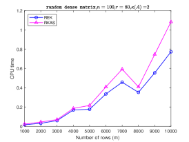
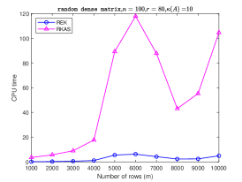
Figure 4. Figures depict the CPU time (in seconds) vs increasing number of rows for the case of the random dense matrix. The title of each plot indicates the values of $n,r$, and $\kappa$. All plots are averaged over 50 trials.

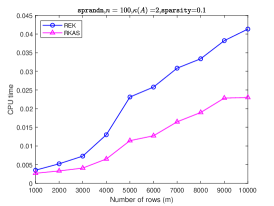
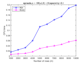
Figure 5. Figures depict the CPU time (in seconds) vs increasing number of rows for the case of the random sparse matrix. The title of each plot indicates the values of $n$, $\kappa$, and sparsity. All plots are averaged over 50 trials.

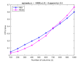
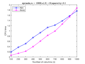
Figure 6. Figures depict the CPU time (in seconds) vs increasing number of columns for the case of the random sparse matrix. The title of each plot indicates the values of $m$, $\kappa$, and sparsity. All plots are averaged over 50 trials.

4.2. Real-world data

The real-world data are available via the SuiteSparse Matrix Collection [25]. The five matrices are nemsafm, df2177, ch8_8_b1, bibd_16_8, and ash958. Each dataset consists of a matrix $A\in\mathbb{R}^{m\times n}$ and a vector $b\in\mathbb{R}^{m}$. In our experiments, we only use the matrices $A$ of the datasets and ignore the vector $b$. In Table 2, we report the number of iterations and the computing times for REK and RKAS. It can be observed that RKAS is comparable with REK for solving inconsistent linear systems.

Table 2. The average (50 trials of each algorithm) Iter and CPU of REK and RKAS for inconsistent linear systems with coefficient matrices from [25].

Matrix	$m\times n$	rank	$\frac{\sigma_{\max}(A)}{\sigma_{\min}(A)}$	REK		RKAS
				Iter	CPU	Iter	CPU
nemsafm	$334\times 2348$	334	4.77	41308.70	1.3104	120565.48	2.3087
df2177	$630\times 10358$	630	2.01	20192.62	5.1010	21480.34	2.9148
ch8_8_b1	$1568\times 64$	63	3.48e+14	1800.96	0.0186	1686.84	0.0136
bibd_16_8	$120\times 12870$	120	9.54	7859.60	3.3143	151632.30	32.4403
ash958	$958\times 292$	292	3.20	15711.02	0.1037	42197.00	0.1924

5. Concluding remarks

Consider the following the least-squares problem

(11) $$\min\limits_{x\in\mathbb{R}^{n}}f(x):=\frac{1}{2m}\|Ax-b\|_{2}^{2}=\frac{1}{m}\sum_{i=1}^{m}f_{i}(x),$$

where $f_{i}(x)=\frac{1}{2}\left(A_{i,:}x-b_{i}\right)^{2}$. To state conveniently, we assume that $A\in\mathbb{R}^{m\times n}$ is normalized to $\|A_{i,:}\|^{2}_{2}=1$ for each row of $A$. The RK method (2) can be seen as stochastic gradient descent (SGD) [21, 44, 29] applied to the least-squares problem (11). Indeed, SGD solves (11) using unbiased estimates for the gradient of the objective function, i.e. $\nabla f_{i}(x)$ such that $\mathbb{E}\left[\nabla f_{i}(x)\right]=\nabla f(x)$. At each iteration, a random unbiased estimate $\nabla f_{i}(x)$ is drawn and SGD uses the following update formula

(12) $$x^{k+1}=x^{k}-\lambda_{k}\nabla f_{i}(x^{k}),$$

where $\lambda_{k}$ is an appropriately chosen stepsize. Noting that if a random row of the matrix $A$ is selected and (12) is computed with $\nabla f_{i}(x^{k})=\left(A_{i,:}x^{k}-b_{i}\right)A_{i,:}^{\top}$, then one can recover the RK method.

It is well-known that SGD suffers from slow convergence as the variance of the gradient estimate $\nabla f_{i}(x)$ does not naturally diminish, i.e. $\lim\limits_{k\rightarrow\infty}\mathbb{E}[\|\nabla f_{i_{k}}(x^{k})-\nabla f(x^{k})\|^{2}_{2}]\neq 0$. Let $x_{*}$ be an optimal point of (11) and consider the variance of its gradient estimate

$$\sigma^{2}=\mathbb{E}[\|\nabla f_{i}(x_{*})-\nabla f(x_{*})\|^{2}_{2}]=\mathbb{E}[\|\nabla f_{i}(x_{*})\|^{2}_{2}]=\sum\limits_{i=1}^{m}\frac{(A_{i,:}x_{*}-b_{i})^{2}}{m}=\frac{\|e\|^{2}_{2}}{m},$$

where $e=Ax_{*}-b$ is the residual at $x_{*}$. When the system is consistent, as the iterate approaches $x_{*}$, the residual gradually drops to zero and thus so does the variance, which ensures the convergence of SGD with a constant stepsize. When the system is inconsistent, however, $e\neq 0$ and the variance does not decrease to zero. In this case, variance reduction techniques are introduced [39, 23], otherwise a decreasing stepsize is required. Nevertheless, the decreasing stepsize brings about adverse effect on the convergence of SGD, which is sublinear even if the objective function is strongly convex [38]. In this paper, we have shown that RK, i.e. SGD for (11), with our adaptive stepsize strategy enjoys a linear rate without any variance reduction procedure. A natural extension of our results is the design and analysis of adaptive stepsizes for SGD in the case of general convex or strongly convex functions. This should be an interesting and valuable topic that deserves in-depth study in the future.

Finally, we note that a bunch of advanced probability criteria have been investigated in the literature for the RK method, such as the greedy selection rule [2] and the weighted version [46]. These criteria are convenient to be adapted to the RKAS context for further improvement in efficiency.

References

- [1] Zhong-Zhi Bai, Lu Wang, and Wen-Ting Wu. On convergence rate of the randomized Gauss–Seidel method. Linear Algebra Appl., 611:237–252, 2021.
- [2] Zhong-Zhi Bai and Wen-Ting Wu. On greedy randomized Kaczmarz method for solving large sparse linear systems. SIAM J. Sci. Comput., 40(1):A592–A606, 2018.
- [3] Zhong-Zhi Bai and Wen-Ting Wu. On partially randomized extended Kaczmarz method for solving large sparse overdetermined inconsistent linear systems. Linear Algebra Appl., 578:225–250, 2019.
- [4] Zhong-Zhi Bai and Wen-Ting Wu. On greedy randomized augmented Kaczmarz method for solving large sparse inconsistent linear systems. SIAM J. Sci. Comput., 43(6):A3892–A3911, 2021.
- [5] Adi Ben-Israel and Thomas NE Greville. Generalized inverses: theory and applications, volume 15. Springer Science & Business Media, 2003.
- [6] Charles Byrne. A unified treatment of some iterative algorithms in signal processing and image reconstruction. Inverse Problems, 20(1):103–120, 2003.
- [7] Yair Censor, Paul PB Eggermont, and Dan Gordon. Strong underrelaxation in Kaczmarz’s method for inconsistent systems. Numer. Math., 41(1):83–92, 1983.
- [8] Kai-Wei Chang, Cho-Jui Hsieh, and Chih-Jen Lin. Coordinate descent method for large-scale L2-loss linear support vector machines. J. Mach. Learn. Res., 9(7):1369––1398, 2008.
- [9] Xuemei Chen and Jing Qin. Regularized Kaczmarz algorithms for tensor recovery. SIAM J. Imaging Sci., 14(4):1439–1471, 2021.
- [10] Kui Du. Tight upper bounds for the convergence of the randomized extended Kaczmarz and Gauss-Seidel algorithms. Numer. Linear Algebra Appl., 26(3):e2233, 2019.
- [11] Kui Du, Wu-Tao Si, and Xiao-Hui Sun. Randomized extended average block Kaczmarz for solving least squares. SIAM J. Sci. Comput., 42(6):A3541–A3559, 2020.
- [12] Kui Du and Xiao-Hui Sun. Pseudoinverse-free randomized block iterative algorithms for consistent and inconsistent linear systems. arXiv preprint arXiv:2011.10353, 2020.
- [13] Hans Georg Feichtinger, C Cenker, M Mayer, H Steier, and Thomas Strohmer. New variants of the POCS method using affine subspaces of finite codimension with applications to irregular sampling. In Visual Communications and Image Processing’92, volume 1818, pages 299–310. SPIE, 1992.
- [14] Gene H Golub and Charles F Van Loan. Matrix computations. JHU press, 2013.
- [15] Richard Gordon, Robert Bender, and Gabor T Herman. Algebraic reconstruction techniques (ART) for three-dimensional electron microscopy and X-ray photography. J. Theor. Biol., 29(3):471–481, 1970.
- [16] Robert M Gower, Denali Molitor, Jacob Moorman, and Deanna Needell. On adaptive sketch-and-project for solving linear systems. SIAM J. Matrix Anal. Appl., 42(2):954–989, 2021.
- [17] Robert M. Gower and Peter Richtárik. Randomized iterative methods for linear systems. SIAM J. Matrix Anal. Appl., 36(4):1660–1690, 2015.
- [18] Deren Han, Yansheng Su, and Jiaxin Xie. Randomized Douglas-Rachford method for linear systems: Improved accuracy and efficiency. arXiv preprint arXiv:2207.04291, 2022.
- [19] Deren Han and Jiaxin Xie. On pseudoinverse-free randomized methods for linear systems: Unified framework and acceleration. arXiv preprint arXiv:2208.05437, 2022.
- [20] Martin Hanke and Wilhelm Niethammer. On the acceleration of Kaczmarz’s method for inconsistent linear systems. Linear Algebra Appl., 130:83–98, 1990.
- [21] Moritz Hardt, Ben Recht, and Yoram Singer. Train faster, generalize better: Stability of stochastic gradient descent. In Proc. 33th Int. Conf. Machine Learning, pages 1225–1234. PMLR, 2016.
- [22] Gabor T Herman and Lorraine B Meyer. Algebraic reconstruction techniques can be made computationally efficient (positron emission tomography application). IEEE Trans. Medical Imaging, 12(3):600–609, 1993.
- [23] Rie Johnson and Tong Zhang. Accelerating stochastic gradient descent using predictive variance reduction. In Proc. Adv. Neural Inf. Process. Syst., pages 315–323, 2013.
- [24] S Karczmarz. Angenäherte auflösung von systemen linearer glei-chungen. Bull. Int. Acad. Pol. Sic. Let., Cl. Sci. Math. Nat., pages 355–357, 1937.
- [25] Scott P Kolodziej, Mohsen Aznaveh, Matthew Bullock, Jarrett David, Timothy A Davis, Matthew Henderson, Yifan Hu, and Read Sandstrom. The suitesparse matrix collection website interface. J. Open Source Softw., 4(35):1244, 2019.
- [26] Dennis Leventhal and Adrian S Lewis. Randomized methods for linear constraints: convergence rates and conditioning. Math. Oper. Res., 35(3):641–654, 2010.
- [27] Ji Liu and Stephen Wright. An accelerated randomized Kaczmarz algorithm. Math. Comp., 85(297):153–178, 2016.
- [28] Nicolas Loizou and Peter Richtárik. Momentum and stochastic momentum for stochastic gradient, newton, proximal point and subspace descent methods. Comput. Optim. Appl., 77(3):653–710, 2020.
- [29] Anna Ma and Deanna Needell. Stochastic gradient descent for linear systems with missing data. Numer. Math. Theory Methods Appl., 12(1):1–20, 2019.
- [30] Anna Ma, Deanna Needell, and Aaditya Ramdas. Convergence properties of the randomized extended Gauss–Seidel and Kaczmarz methods. SIAM J. Matrix Anal. Appl., 36(4):1590–1604, 2015.
- [31] Jacob D Moorman, Thomas K Tu, Denali Molitor, and Deanna Needell. Randomized Kaczmarz with averaging. BIT., 61(1):337–359, 2021.
- [32] Frank Natterer. The mathematics of computerized tomography. SIAM, 2001.
- [33] Ion Necoara. Faster randomized block Kaczmarz algorithms. SIAM J. Matrix Anal. Appl., 40(4):1425–1452, 2019.
- [34] Deanna Needell. Randomized Kaczmarz solver for noisy linear systems. BIT., 50(2):395–403, 2010.
- [35] Deanna Needell, Nathan Srebro, and Rachel Ward. Stochastic gradient descent, weighted sampling, and the randomized Kaczmarz algorithm. Math. Program., 155:549–573, 2016.
- [36] Deanna Needell and Joel A Tropp. Paved with good intentions: analysis of a randomized block kaczmarz method. Linear Algebra Appl., 441:199–221, 2014.
- [37] Deanna Needell and Rachel Ward. Two-subspace projection method for coherent overdetermined systems. J. Fourier Anal. Appl., 19(2):256–269, 2013.
- [38] Arkadi Nemirovski, Anatoli Juditsky, Guanghui Lan, and Alexander Shapiro. Robust stochastic approximation approach to stochastic programming. SIAM J. Optim., 19(4):1574–1609, 2009.
- [39] Lam M Nguyen, Jie Liu, Katya Scheinberg, and Martin Takáč. Sarah: A novel method for machine learning problems using stochastic recursive gradient. In Proc. 34th Int. Conf. Machine Learning, pages 2613–2621. PMLR, 2017.
- [40] Maxim A Olshanskii and Eugene E Tyrtyshnikov. Iterative methods for linear systems: theory and applications. SIAM, 2014.
- [41] Andrei Patrascu and Ion Necoara. Nonasymptotic convergence of stochastic proximal point methods for constrained convex optimization. J. Mach. Learn. Res., 18(1):7204–7245, 2017.
- [42] Constantin Popa. Extensions of block-projections methods with relaxation parameters to inconsistent and rank-deficient least-squares problems. BIT., 38(1):151–176, 1998.
- [43] Constantin Popa. Characterization of the solutions set of inconsistent least-squares problems by an extended Kaczmarz algorithm. Korean J. Comput. Appl. Math., 6(1):51–64, 1999.
- [44] Herbert Robbins and Sutton Monro. A stochastic approximation method. Ann. Math. Statistics, pages 400–407, 1951.
- [45] Frank Schöpfer and Dirk A Lorenz. Linear convergence of the randomized sparse Kaczmarz method. Math. Program., 173(1):509–536, 2019.
- [46] Stefan Steinerberger. A weighted randomized Kaczmarz method for solving linear systems. Math. Comp., 90:2815–2826, 2021.
- [47] Thomas Strohmer and Roman Vershynin. A randomized Kaczmarz algorithm with exponential convergence. J. Fourier Anal. Appl., 15(2):262–278, 2009.
- [48] Nian-Ci Wu, Chengzhi Liu, Yatian Wang, and Qian Zuo. On the extended randomized multiple row method for solving linear least-squares problems. arXiv preprint arXiv:2210.03478, 2022.
- [49] Nian-Ci Wu and Hua Xiang. Semiconvergence analysis of the randomized row iterative method and its extended variants. Numer. Linear Algebra Appl., 28(1):e2334, 2021.
- [50] Wen-Ting Wu. On two-subspace randomized extended Kaczmarz method for solving large linear least-squares problems. Numer. Algorithms, 89(1):1–31, 2022.
- [51] Anastasios Zouzias and Nikolaos M. Freris. Randomized extended Kaczmarz for solving least squares. SIAM J. Matrix Anal. Appl., 34(2):773–793, 2013.