Mapping the whole-brain effective connectome with excitatory-inhibitory causal relationship

Abstract

Understanding the large-scale causal relationship among brain regions is crucial for elucidating the information flow that the brain integrates external stimuli and generates behaviors. Despite the availability of neurostimulation and computational methods to infer causal relationships among a limited number of regions, these approaches are not capable of mapping the causal network of the entire brain, also known as the effective brain connectome (EBC). To address this gap, we propose a data-driven framework called Neural Perturbational Inference (NPI) and map the human EBC for the first time. NPI uses an artificial neural network trained to learn large-scale neural dynamics as a surrogate brain. By perturbing each region of the surrogate brain and observing the resulting responses in all other regions, the human EBC is obtained. This connectome captures the directionality, strength, and excitatory-inhibitory distinction of brain-wide causal relationships, offering mechanistic insights into cognitive processes. EBC provides a complete picture of information flow both within and across brain functional networks as well as reveals the large-scale hierarchy of the organization of excitatory and inhibitory ECs. As EBC captures the neurostimulation transmission pathways in the brain, it has great potential to guide the target selection in personalized neurostimulation of neurological disorders.

1 Introduction

The brain is a complex network of interconnected regions that work in concert to integrate information from the environment with internal dynamic states and generate a wide range of behaviors Park2013Structural . Understanding the flow of information among brain regions is essential for comprehending the connection between stimuli and responses. However, current measures of macroscopic inter-region connections, such as structural connectivity (SC) and functional connectivity (FC), fall short of providing information flow within the brain and thus limit the mechanistic understanding of brain functions. SC provides a static representation of physical connections but fails to capture the dynamic nature of brain function Yeh2021Mapping . FC examines statistical associations among regional neural signals but is still not a causal relationship vandenHeuvel2010Exploring . Therefore, it is necessary to measure the effective connectivity (EC), which captures the positive or negative causal impact a given region can have on its downstream regions, thereby depicting the flow of information Schippers2010Mapping . Despite the availability of methods that infer EC among a few regions, a whole-brain EC, which we call the effective brain connectome (EBC), is still lacking. In order to understand the complete information flow from receiving external information to multi-sensory integration and behavior generation, an accurate EBC is desperately in need.

Experimental manipulation is a straightforward and widely used approach to examine the input-output causality, which is also the EC, among brain regions Pearl2009Causality . By manipulating a specific brain region and simultaneously observing the induced effects at other regions, it provides direct evidence of causality Veit2021Temporal ; Ozdemir2020Individualized . Several manipulation techniques, such as electrical stimulations and optogenetics, and observation techniques, including electroencephalogram (EEG) and functional magnetic resonance imaging (fMRI), have been applied for mapping causal relationships Keller2014Mapping ; Bauer2018Effective . However, there are technical gaps to map EBC by experimental manipulations. The invasive neurostimulation techniques is hard to be performed at many brain regions. Concurrent stimulation and neural responses observation is also not feasible at the whole-brain scale. Computational approaches provide alternative solutions, which infer EC from regional neural signals with both model-based and model-free methods Friston2014DCM ; Barnett2014MVGC . However, existing computational methods still have limited ability to offer an accurate EBC. Model-based methods, such as dynamic causal modeling (DCM), rely heavily on model assumptions and thus suffer from inference biases due to the model mismatch. Model-free methods that are typically based on statistics, such as Granger Causality, characterize the direction of EC but is often hard to determine the strength and excitatory-inhibitory distinction of EC Li2018Causal . Moreover, as the meaning of EC varies across computational frameworks, how they relate to EC obtained by experimental neuromodulation is still unclear. As a result, human EBC is still lacking.

With the proliferation of big data in neuroscience, such as brain imaging or electrophysiological recordings, an increasing number of studies are employing artificial neural networks (ANNs) to unveil hidden information from these vast neural data Lundervold2019overview . Applications encompass neural decoding, neuroimaging reconstruction, and the diagnosis and control of neurological disorders Pandarinath2018Inferring ; Yan2020Reconstructing ; Liang2022Online . Despite the remarkable fitting capabilities of ANNs, for example, a recurrent neural network (RNN) well-tracking the nonlinear dynamics of a few nodes Kim2021Teaching , training an ANN to capture the large-scale brain dynamics and to represent its underlying connectivity structure remains a challenge. Previous studies have shown that perturbing the input variables of ANN and monitoring alterations in output enables the identification of the causal relationship between a specific input and the output Samek2021Explaining . Such perturbation-based procedure in ANN is analogous to deriving causal relationships through experimental intervention Veit2021Temporal ; Ozdemir2020Individualized . Enlightened by this analogy, we incorporate the perturbation-based experiments into a data-driven framework to study the causality in the brain. Once the ANN is trained to capture the brain-wide neural dynamics, systematically perturbing this ANN can yield a map of causal relationships among all brain regions, which is the human EBC.

Here, we present a novel approach called Neural Perturbational Inference (NPI). NPI trains an ANN to accurately model brain dynamics and then uses it as a surrogate brain to be perturbed. The whole-brain EC is then obtained by perturbing the surrogate brain region by region while simultaneously observing the resulting neural responses in all other regions. We applied NPI to human resting-state fMRI (rsfMRI) signals and obtained the human EBC for the first time. The inferred EBC exhibits whole-brain causal interactions with directionality, strength, and the excitatory-inhibitory distinction, providing a comprehensive view of macroscopic resting-state information flow within and across functional networks. It uncovers the neural mechanism under cognitive processes and deepens our understanding of brain structure-function relationship. In addition, since EBC reflects the transmission pathway of neurostimulation, it has great potential in guiding the target selection in neuromodulation such as in personalized treatment of neurological and psychiatric diseases.

2 Results

2.1 The NPI framework

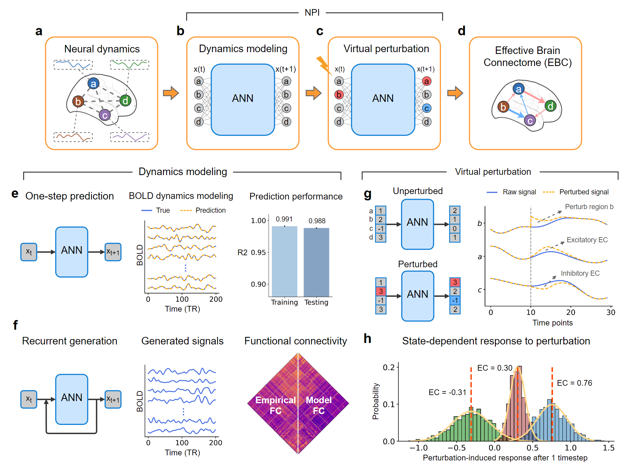
Figure 1: The NPI framework for inferring EBC. (a) Schematic of the brain network and the neural signal of each brain region. The EBC among regions is unknown and to be inferred. (b) A surrogate brain, an ANN, is trained to replace the real brain to be perturbed. The ANN model is trained to capture brain dynamics in terms of predicting the next brain state $\mathbf{x}(t+1)$ given the current brain state $\mathbf{x}(t)$. (c) After training, ANN is systematically perturbed to infer EC. Perturbation is applied as a selective increase of neural signal at one region. The red background indicates an increase in neural signal compared with not applying perturbation, while the blue indicates a decrease. After perturbing one region, the magnitude of the one-step responses refers to a one-to-all EC. (d) The all-to-all EC (EBC) can be inferred by perturbing the ANN region by region. This EBC is a brain-wide map of causal influences that has directionality, strength, and excitatory-inhibitory distinction. (e) ANN trained on individual data accurately models BOLD dynamics. The $r^{2}$ of one-step prediction using ANN is near 1.0 on both the training (0.991) and testing (0.988) data. (f) Recurrently feeding the result of one-step prediction as input to ANN produces the generated neural signals. The model FC and empirical FC are respectively calculated from generated BOLD signals and empirical BOLD signals and are averaged across 800 subjects. They are highly correlated with a correlation coefficient of 0.97. (g) After perturbing region $b$, the increased signal in the region $a$ and decreased signal in the region $c$ indicate an excitatory EC from $b$ to $a$, and an inhibitory EC from $b$ to $c$. (h) The response to a perturbation is state-dependent. We perturb the ANN at different brain states and take the averaged response to be EC. The distribution of three ECs of one subject is demonstrated. Green bars show the response of left V1 after perturbing left OFC ($mean=-0.31,std=0.25$), brown one shows the response of left V3 after perturbing left V2 ($mean=0.30,std=0.10$), and the blue one shows the response of right V1 after perturbing left V1 ($mean=0.76,std=0.20$).

NPI is a framework that non-invasively infers EBC from neural signals (Fig. 1). From brain imaging or electrophysiological recordings, the collective neural activities of multiple brain regions are easily available, but how these regions interact to process information is unclear (Fig. 1 a). NPI aims to infer EC among regions in the entire brain, which are directed causal connections. Experimental perturbations such as electrical and magnetic stimulations have widely been used to map EC among a few brain regions Keller2014Mapping . To enable brain-wide perturbation and avoid physically stimulating the real brain, NPI uses a data-driven approach to infer EC. Conceptually, NPI is similar to perturbing the real brain through neurostimulation, but it uses an ANN as a surrogate brain to replace the real brain, which enables efficient whole-brain perturbation and observation (Fig. 1b). This study implements the ANN as a multi-layer perceptron. The ANN is trained to predict brain state at the next time step based on the brain state at the current step by minimizing the one-step-ahead prediction error. After training, the ANN is treated as a surrogate brain. It is then systematically perturbed to extract the underlying EC (Fig. 1c). By perturbing a source region and observing the response of target region at the next time step, the EC from the source region to the target region is inferred based on the change in predicted neural activity with and without perturbation. Systematically perturbing each node in ANN reveals the EBC (Fig. 1d), which characterizes the directionality, strength, and excitatory-inhibitory distinction of the causal influences among all brain regions. It represents the extent to which one brain region can positively or negatively influence others.

The ANN in NPI exhibits a high ability to model fMRI dynamics, using rsfMRI data from 800 subjects in the Human Connectome Project (HCP) dataset VanEssen2013WU-Minn . After separate ANN training for each subject, the ANN in NPI accurately learns the mapping between two consecutive BOLD signals, as indicated by the coefficient of determination ($r^{2}$) that are close to 1 for both the training ($r^{2}=0.991$) and the testing data ($r^{2}=0.988$) (Fig. 1e). Besides the accurate one-step prediction, the ANN model also captures the interaction relationships among brain regions. We recursively feed the predicted signals back into the ANN model and generate the synthetic BOLD signals over 200 time steps (Fig. 1f). The FC calculated from the generated BOLD signals (model FC) and FC calculated from the empirical BOLD signals (empirical FC) are compared, both of which are averaged across 800 subjects. The model FC and empirical FC are strongly correlated ($r=0.98$, $p\leq 10^{-4}$), suggesting ANN captures the dynamic relationship among brain regions. Together, the evidence from accurate one-step prediction and FC recovery suggest that the trained ANN model is valid to serve as a surrogate brain for virtual perturbation experiments.

The parameters in ANN are fixed after training. Perturbations are then applied to explore the underlying causal relationships among nodes. In the ANN, the perturbation is implemented as an increase in the neural activity of a particular source node, while keeping the neural signals of other target nodes unchanged. Both the perturbed and unperturbed signals are input to the ANN, which maps the corresponding next state of the neural signals. The difference in the next state of target regions given the perturbed and unperturbed current state is measured as the EC from the source node to target nodes. Compared with the next state without perturbation, an increased activity of a target region after perturbation indicates an excitatory EC from the source node to the target node, while a decrease indicates an inhibitory EC (Fig. 1f). Since the nonlinear nature of brain dynamics, the response to perturbation varies with the initial states. This is similar to the state-dependent response happened in real stimulation Scangos2021Statedependent . We thus calculate the averaged response after applying perturbations at multiple initial states as the final EC (Fig. 1g).

2.2 Validation of NPI using an RNN model

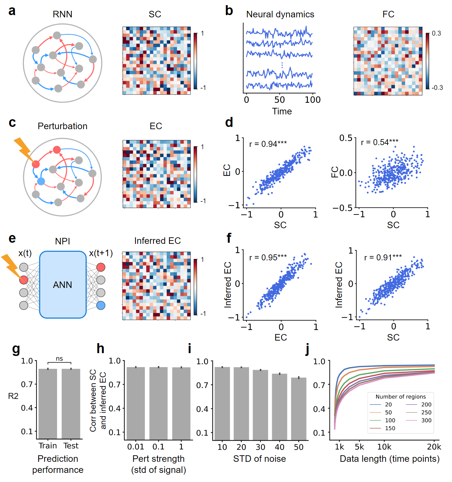
Figure 2: Validation of NPI using an RNN model To validate the effectiveness of NPI, we test its ability to recover ground-truth SC using synthetic data generated from an RNN model with known SC. (a) The RNN model with SC sampled from a Gaussian distribution with zero mean value. The maximum weight in SC is scaled to 1. (b) The synthetic neural dynamics are generated by the RNN model. FC is then calculated from the generated signals. (c) The output EC of a source node is obtained as the magnitude of response at target nodes after perturbing this source node. Perturbing all nodes in turn offers an all-to-all EC. The maximum weight is scaled to 1. (d) Both EC ($r=0.94,p\leq 10^{-3}$) and FC ($r=0.54,p\leq 10^{-3}$) of RNN are strongly correlated with SC of RNN. EC better reconstructs SC than FC. (e) NPI infers the EC of RNN from generated neural signals by training and perturbing a surrogate ANN trained to learn the neural dynamics in RNN. (f) The inferred EC is strongly correlated with EC obtained by direction perturbing the RNN model and the ground-truth SC in RNN. (g) The ability of ANN in predicting the RNN signal at the next time step is assessed by the coefficient of determination. The training set is constructed using consecutive pairs in generated neural signals as in (b). The testing set is constructed by the resulting neural activities produced by perturbing the signal of a region and mapping the next step using the RNN model. (h) The inference performance is robust against the magnitude of the perturbation (compared with the standard deviation of the signal). (i) The inference performance is robust against the standard deviation of the system noise. (j) With the increasing number of regions, NPI needs more data to achieve a good inference performance.

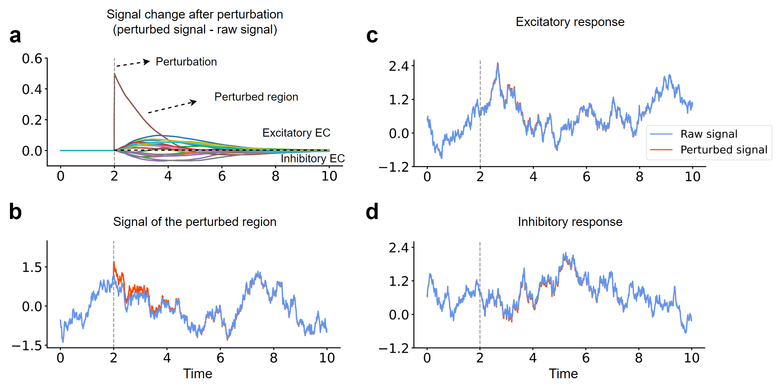
Figure S7: The signal change in RNN after perturbing a region. (a) The perturbation-induced signal changes of all regions are calculated as the difference between the signals with and without perturbation. Regions that have excitatory input EC from the perturbed region exhibit positive responses. Regions that have inhibitory input EC from the perturbed region exhibit negative responses. (b) Signal of the perturbed region. (c) Signal of a region that has excitatory input EC from the perturbed region. (d) Signal of a region that has inhibitory input EC from the perturbed region.

To show the effectiveness of NPI framework in recovering the underlying EC, NPI is applied to recover the EC from the dynamics generated by an RNN model with known ground-truth SC. A single-layer RNN is used with the weight matrix (the SC of RNN) randomly sampled from a Gaussian distribution with zero mean value (Fig. 2 a). The FC of neural dynamics is calculated as the Pearson’s correlation among regional signals. The obtained FC is correlated with the ground-truth SC with the coefficient $0.54$ (Fig. 2b,d). The EC of the RNN model can be obtained by directly perturbing the model (Fig. 2c). Perturbing a region is implemented as an increase in the neural signal of this region. After a time step, the averaged changes in neural signals of other regions are calculated as the strengths of EC from the perturbed region to other regions, with the maximum EC scaled to 1 (Fig. S7). Since the state-dependence of perturbation-induced response, the averaged response after perturbing at $1000$ randomly chosen initial states is calculated as the final EC. The resulting EC is strongly correlated with SC ($r=0.94$), which is reasonable since EC is constrained by SC (Fig. 2d). Due to the modulation of nonlinear brain dynamics and the noise in the neural signals, EC does not exactly equal to SC. Despite that, the correlation between EC and SC is much higher than that between FC and SC, which may result from the spurious connections and the lack of directionality in FC.

We next examine whether NPI-inferred EC recovers the EC from direct perturbing RNN model and the ground-truth SC. NPI is applied to the RNN generated neural signals to infer EC (Fig. 2e). The NPI-inferred EC is highly correlated with the EC obtained by direct perturbation and is thus also highly correlated with the SC (Fig. 2f). This suggests that the ANN in NPI accurately predicts the response to a perturbation given an particular initial state. This high correlation also validate the effectiveness of NPI for inferring EC from neural dynamics.

To show the direct evidence of the prediction ability of ANN, we examine the ability of ANN in predicting the neural signals at the next step for both training and testing set. The training set consists of consecutive data pairs sampled from generated neural dynamics, as in Fig. 2b. The testing set is constructed by applying perturbations to a region and mapping the next step by the ground-truth RNN model. The signals in the testing set are not sampled from the RNN generated neural dynamics and are thus out-of-distribution (OOD) data. The result shows that the ANN trained on the observed neural signals can also generalize to the OOD testing set (Fig. 2g), which is the foundation of the successful EC inference. The robustness of NPI is also tested with the RNN model. When perturbing the ANN, various perturbation magnitudes are tested and the result shows that the inference performance is robust against the perturbation magnitudes (Fig. 2h). The performance under different levels of system noise is also tested. Despite some decrease in the inference performance with increasing noise, the performance is overall robust (Fig. 2i). When testing NPI on data with different lengths and different numbers of regions, result shows more data is needed to infer EC from the network with a larger number of regions (Fig. 2j).

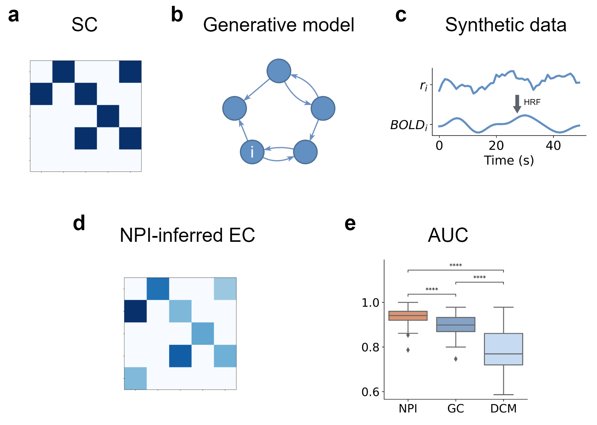
Figure S8: Validation of NPI on a public dataset A publicly available dataset by Sanchez-Romero et al. is used to validate the ability of NPI Sanchez-Romero2019Estimating . (a) In the generative model, the ground truth structural connectivity (SC) is directed and has binary weights, with values of either 0 or 1. (b) The dynamics of firing rates are linear and are constrained by the ground truth SC. (c) The generated neural firing rates are transformed into BOLD signals using an HRF. (d) The EC is inferred by applying NPI to the BOLD signals. (e) The classification accuracy of differentiating between the presence and absence of connections between brain regions is assessed for NPI, as well as two benchmark methods: Granger Causality (GC) and Dynamic Causal Modeling (DCM). The area under the receiver operating characteristic curve (AUC) is calculated as a measure of classification performance. Results showed that NPI had significantly higher AUC compared to the GC ($p\leq 10^{-4}$) and DCM ($p\leq 10^{-4}$).

To validate the ability of NPI on BOLD signals, we apply NPI on a publicly available dataset by Sanchez-Romero et al. Sanchez-Romero2019Estimating , which has been used to validate many EC inference algorithms. The data generation process involves neural firing rate dynamics followed by a hemodynamic response function (HRF) that transforms the neural signals into BOLD signals (Fig. S8). The entries in SC are all binary values (either 0 or 1). We binarize the NPI-inferred EC and compare it with the underlying SC, evaluating its ability to correctly classify the presence or absence of connections. The performance of classification is measured using the area under the receiver operating characteristic curve (AUC). The result shows that the AUC of NPI is very close to 1.0 and NPI performs significantly better than the two baseline EC inference methods (Granger causality and DCM) (Fig. S8e).

2.3 The human EBC inferred by NPI

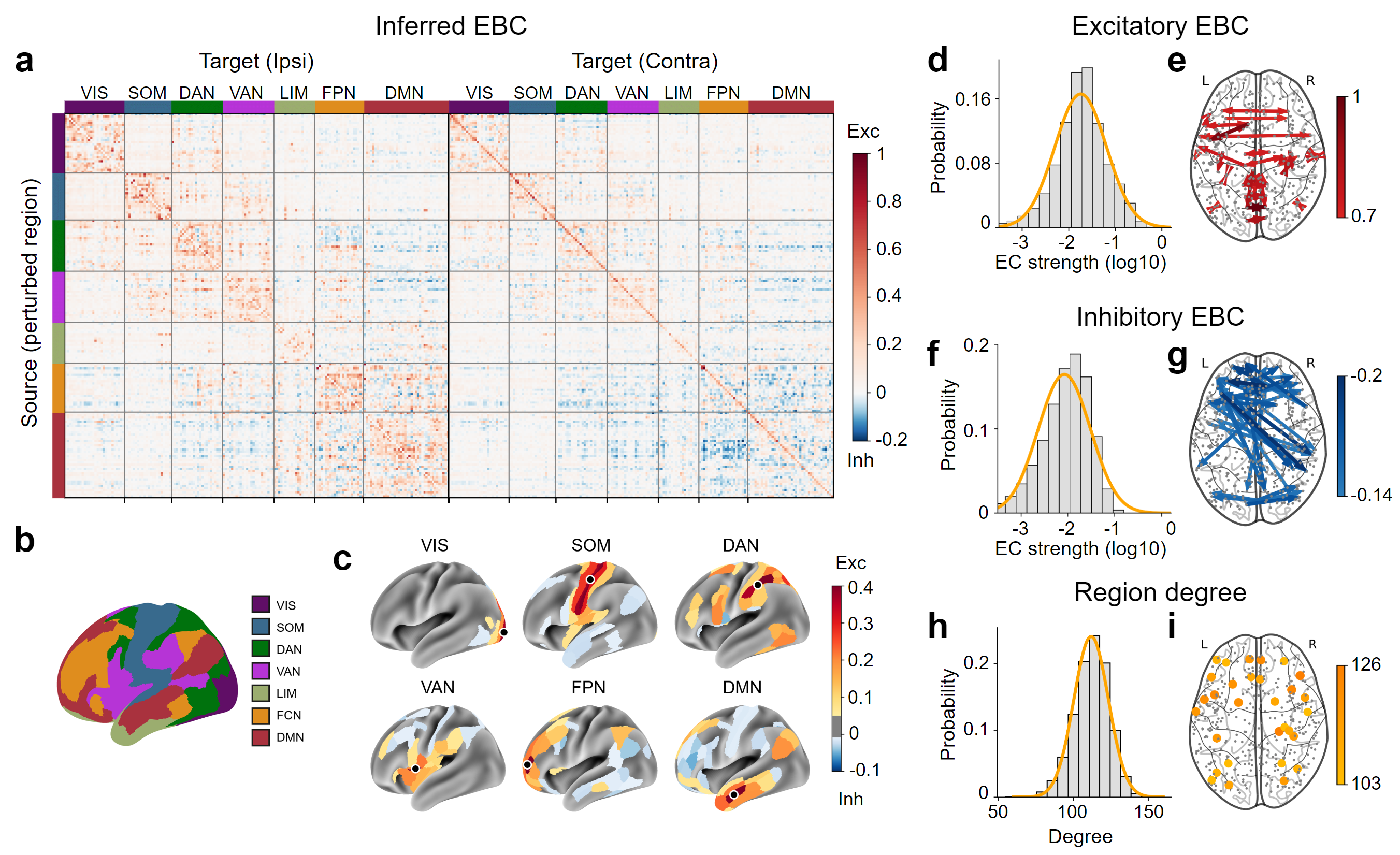
Figure 3: The human EBC. (a) The averaged EBC of 800 subjects, with regions organized according to functional networks. Each row represents the EC from a source region in the left hemisphere to the entire cortex. (b) Cortical areas are assigned to seven functional resting-state networks: visual network (VIS), somatomotor network (SOM), dorsal attention network (DAN), ventral attention network (VAN), limbic network (LIM), frontoparietal network (FPN), and default mode network (DMN). (c) Topological maps of EC from a seed region in seven cortical networks respectively. The seed region is indicated with a black dot on each map. (d,f) The strength of both excitatory (d) and inhibitory (f) EC follows a log-normal distribution, as demonstrated by the fitting curve of log-transformed EC strengths by a Gaussian distribution. (e,g) The 50 strongest excitatory (e) and inhibitory (g) EC. (h) The degree distribution of regions in the binarized EBC. EBC is binarized by a threshold larger than 80% of ECs. The degree is calculated as the mean of the in-degree and out-degree of each region. The in-degree represents the number of input ECs to that region and the out-degree represents the number of output ECs from that region. (i) 30 brain regions with the largest degree after binarizing EBC.

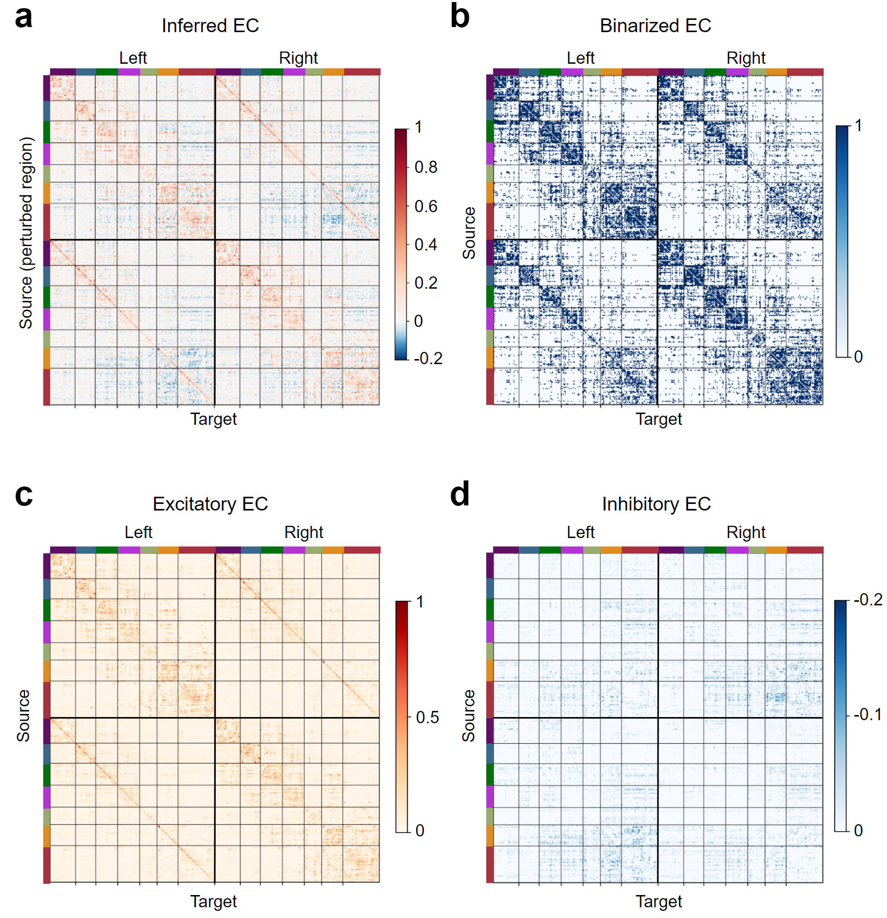
Figure S9: The EBC, binarized EBC, and excitatory and inhibitory part of EBC. (a) The whole-brain EBC. (b) EBC binarized by a threshold larger than 80% of ECs. The entries larger than the threshold are set to 1, while the rest are set to 0. (c,d) The excitatory (c) and inhibitory (d) part of EBC.

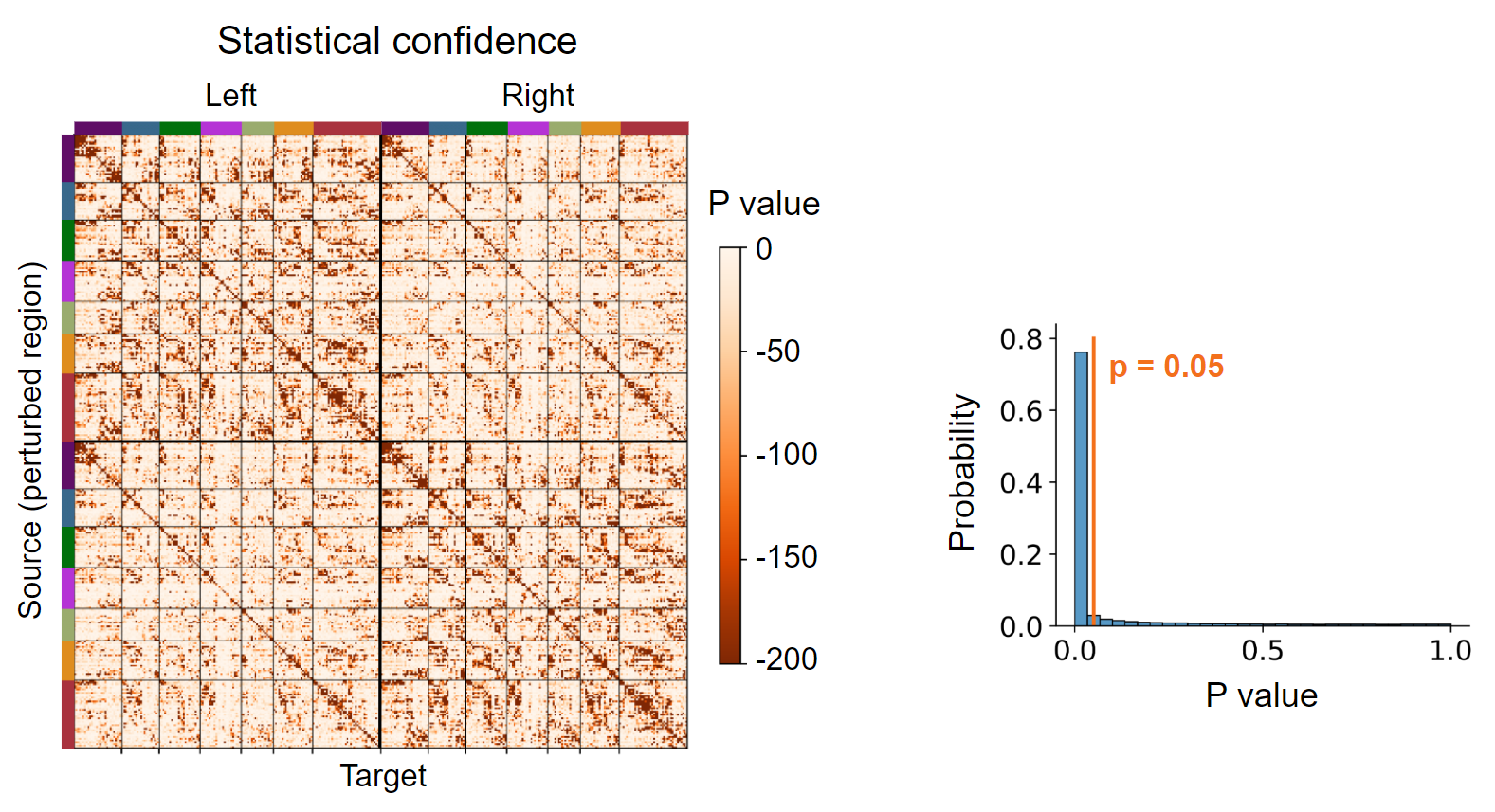
Figure S10: Statistical confidence of EC across individuals. The statistical confidence of whether each connection strength is significantly different from zero based on the EC across 800 subjects. 78% ECs in EBC is significantly different from zero ($p<0.05$, FDR corrected).

We apply NPI to rs-fMRI data from 800 subjects in the HCP dataset. The obtained resting-state EC originating from the left hemisphere is plotted in Fig. 3a with the maximum response scaled to 1 (EC for the entire brain is shown in Fig. S9). The positive entries indicate excitatory EC and negative entries indicate inhibitory EC. The excitatory EC has a maximum strength of $1$, while inhibitory EC has a maximum strength of $0.22$. The brain regions are assigned to seven functional networks (visual network (VIS), somatomotor network (SOM), dorsal attention network (DAN), ventral attention network (VAN), frontoparietal network (FPN), and default mode network (DMN)) according to Yeo et al. ThomasYeo2011organization (Fig. 3b). Among all the EC entries, $78\%$ of the ECs are significantly different from zero (Fig. S10, $p\leq 0.05$, FDR corrected). Seed-based EC is then analyzed to examine the topographic organization of functional networks in EBC. The top 15% excitatory and top 15% inhibitory output ECs from seeds in six functional brain networks are plotted, showing a similar structure as networks defined by FC and revealing more information on how the seed regions inhibit other regions (Fig. 3c).

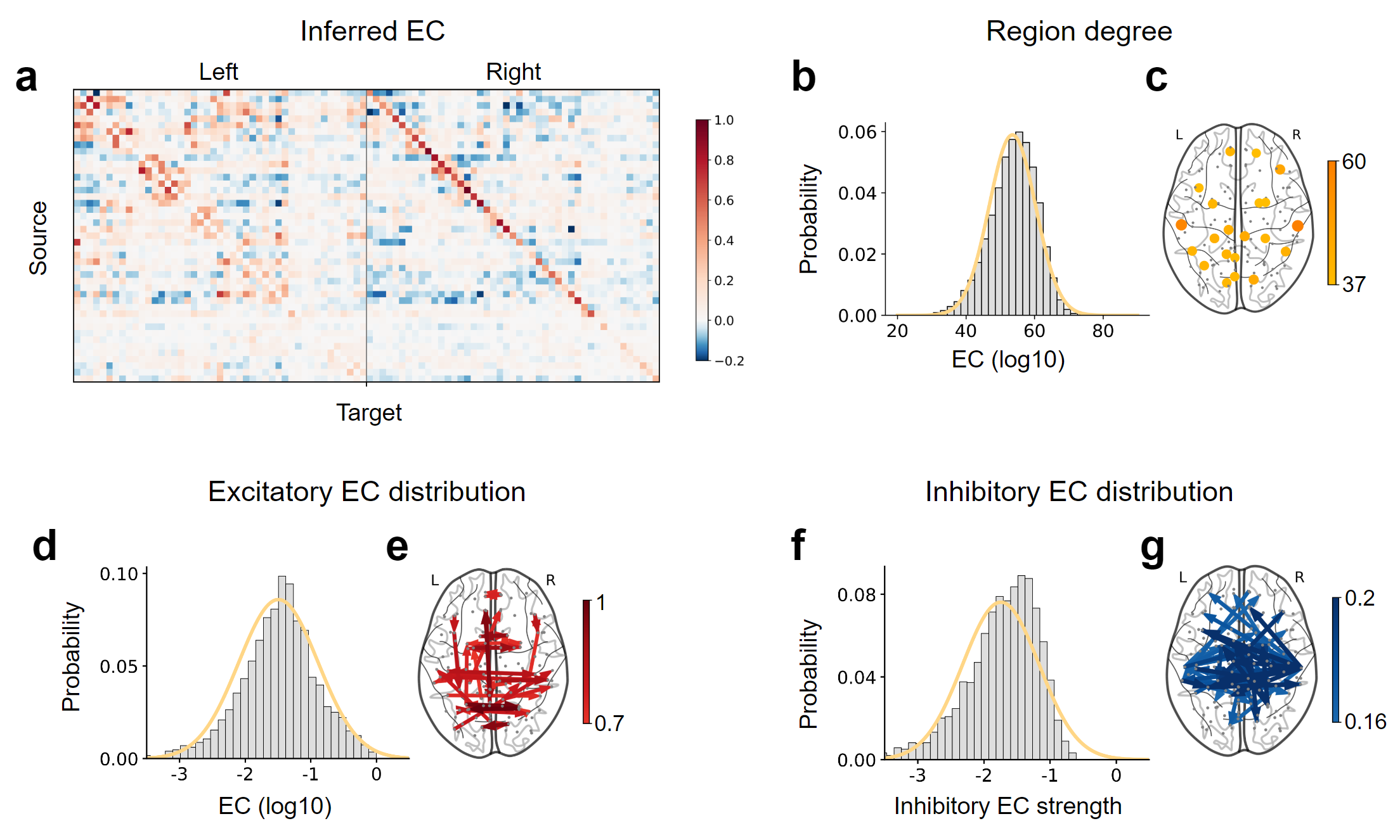
Figure S11: NPI-inferred EBC from the AAL atlas. (a) The inferred EC from the left hemisphere to the whole brain. (b) The degree distribution of regions in the binarized EBC. EBC is binarized by a threshold larger than 80% of ECs. The degree is calculated as the mean of the in-degree and out-degree of each region. (c) 20 brain regions with the largest degree after binarizing EBC. (d, f) The distribution of excitatory (d) and inhibitory (f) EC across the whole brain. The distribution of both can be the best fit by a log-normal distribution. The fitting curves of Gaussian distribution to the log-transformed EC strengths are plotted in yellow. (e,g) The 50 strongest excitatory (e) and inhibitory (g) EC.

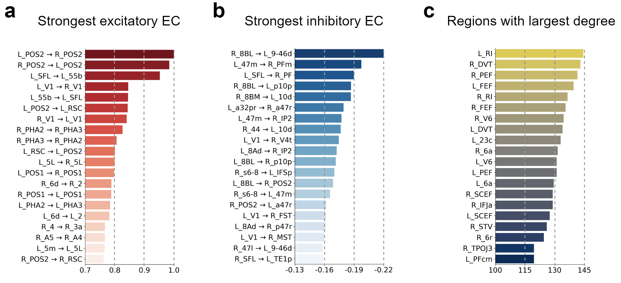
Figure S12: The ECs with strongest strengths and regions with largest degrees. (a,b) The top 20 strongest excitatory (a) EC and inhibitory (b) EC. (c) 20 brain regions with the largest degree after binarizing EBC.

The majority of ECs have small and near-zero strengths, with a few having very large strengths. The distribution shows a long-tail property. We fit the strengths to four hypothesized distributions: log-normal, normal, exponential, and inverse Gaussian. According to the Akaike information criterion (AIC), the log-normal distribution is the best fit for both excitatory and inhibitory ECs, as well as for the combination of absolute strength of them (Fig. 3d,f, S1). It is consistent with the distribution of SC found in experimental studies using tract-tracing techniques involving mice and macaques Oh2014mesoscale ; Markov2014Weighted . The log-normal distributions of excitatory and inhibitory ECs are reproducible under the Automated Anatomical Labeling (AAL) parcellation (Fig. S11). The 50 strongest excitatory and inhibitory ECs are respectively plotted in Fig. 3e,g, and the top 20 strongest excitatory and inhibitory ECs are highlighted in Fig. S12a,b. The strongest excitatory ECs are mostly intra-network connections (41 out of 50), either intra-hemisphere or inter-hemisphere. The strongest inhibitory ECs are mostly inter-network connections (36 out of 50), and are all inter-hemisphere connections. In a network, the degree of a node refers to the number of connections it has with other nodes in the network and can be used to measure the centrality or importance of that node in the network. We binarize the EBC at a threshold that larger than $80\%$ of absolute EC strengths (0.063) (Fig. S9b). The ECs with absolute strengths below the threshold are set to 0, while the rest are set to 1. The excitatory and inhibitory ECs are not differentiated in binarized EBC. Since EC is directed and thus asymmetric, the in-degree of a node is different from the out-degree. In binarized EBC, most of the ECs are bidirectional (73%), consistent with previous findings on SC Felleman1991Distributed . Regions with the largest averaged in-out degrees are plotted in Fig. 3i. They are dispersed across the cortex in several functional networks (Fig. S12c).

2.4 The organization of excitatory and inhibitory ECs across functional networks

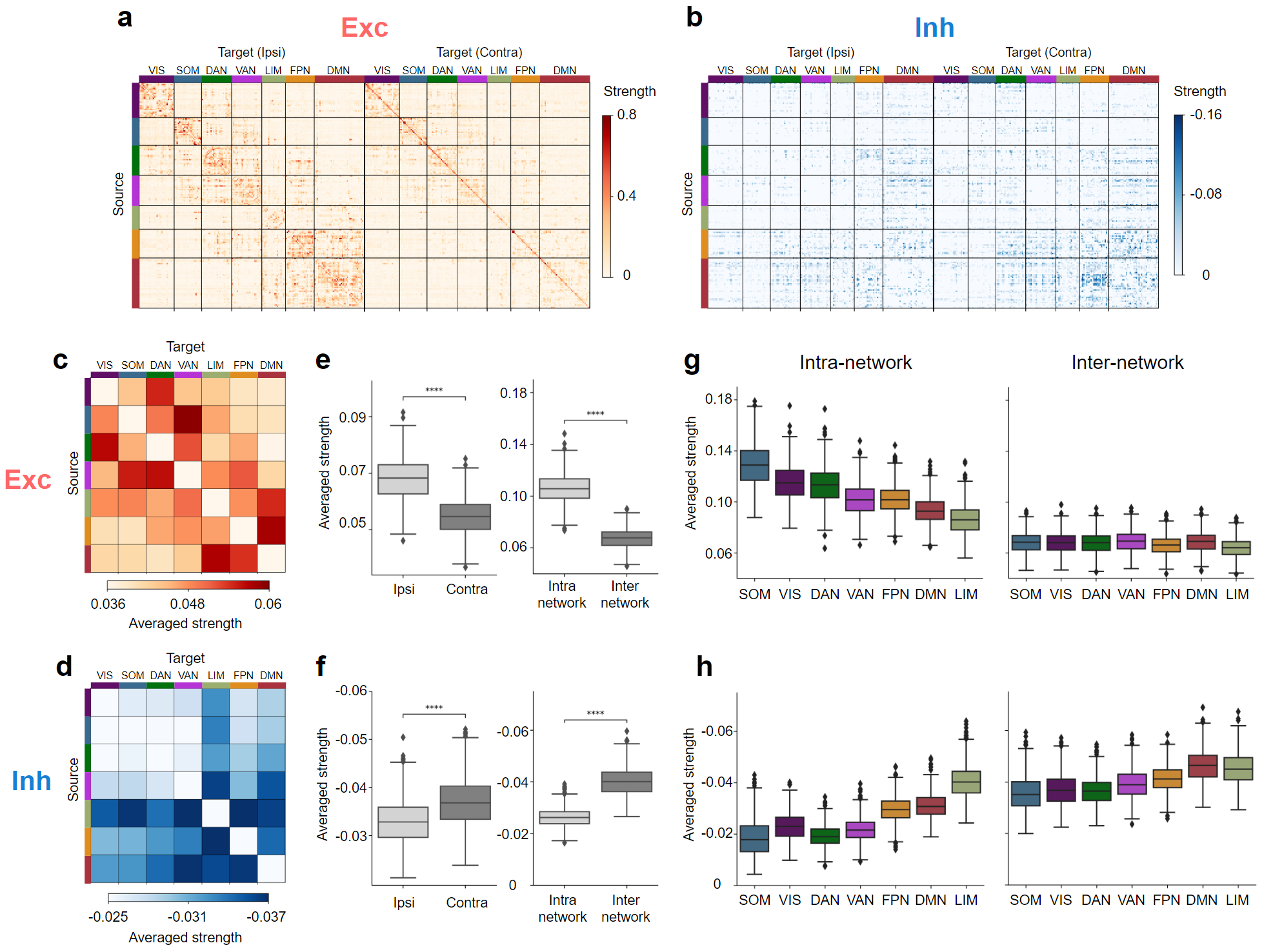
Figure 4: The organization of excitatory and inhibitory ECs across functional networks (a,b) The excitatory (a) and inhibitory (b) parts of EC from the left hemisphere to the whole cortex. (c,d) The averaged excitatory (c) and inhibitory (d) EC strength across seven functional brain networks. (e,f) The averaged excitatory EC strength (e) is higher for ipsi-lateral and intra-network ECs, while the averaged inhibitory EC strength (f) is higher for contra-lateral and inter-network ECs. (g,h) The averaged excitatory (g) and inhibitory (h) EC strength within and across seven functional brain networks. Networks are ordered by the averaged intra-network excitatory EC strength.

EBC distinguishes the excitatory and inhibitory causal influences in large-scale connections for the first time, since previous measures including SC and FC fails to distinguish them. This distinction offers the mechanism under cognitive processes with more details as well as guides the choosing of neurostimulation targets that excite or inhibit the desired regions.

Recent discoveries in both the decomposition of large-scale FC Margulies2016Situating and local measurements across multiple brain areas Murray2014hierarchy have revealed a principal hierarchy of functional differences across cortical areas, spanning from primary sensorimotor networks to higher-order association networks. Here we examine how excitatory (Fig. 4a) and inhibitory (Fig. 4b) ECs are organized across functional brain networks. The averaged excitatory/inhibitory EC strength from network $X$ to network $Y$ is calculated as the total strengths of excitatory/inhibitory EC from regions in $X$ to regions in $Y$ divided by the total number of ECs from regions in $X$ to regions in $Y$. The averaged inter-network EC strength for a particular network is calculated as the average strength from or to that network. The average strength and the maximum strength of excitatory ECs are both higher than that of inhibitory EC. In addition, the excitatory ECs have a higher density for ipsi-lateral and intra-network connections, while inhibitory ECs have a higher density for contra-lateral and inter-network connections (Fig. 4c,d). Within seven networks, the average strength of excitatory and inhibitory ECs are in two opposite hierarchies. The excitatory ECs have higher strengths in primary sensory networks (VIS and SOM) than in association networks (DAN, VAN, FPN, DMN, and LIM), with the highest strengths in the SOM (Fig. 4e,f). The inhibitory ECs, on the other hand, have higher strengths in association networks than in primary sensory networks, with the highest strength in the LIM. The excitatory inter-network ECs have lower strengths compared with intra-network ECs and have similar strengths in seven networks, while inhibitory inter-network ECs have higher strengths and follow a similar hierarchy as intra-network ECs.

2.5 Information flow within DMN and between DMN and cortex

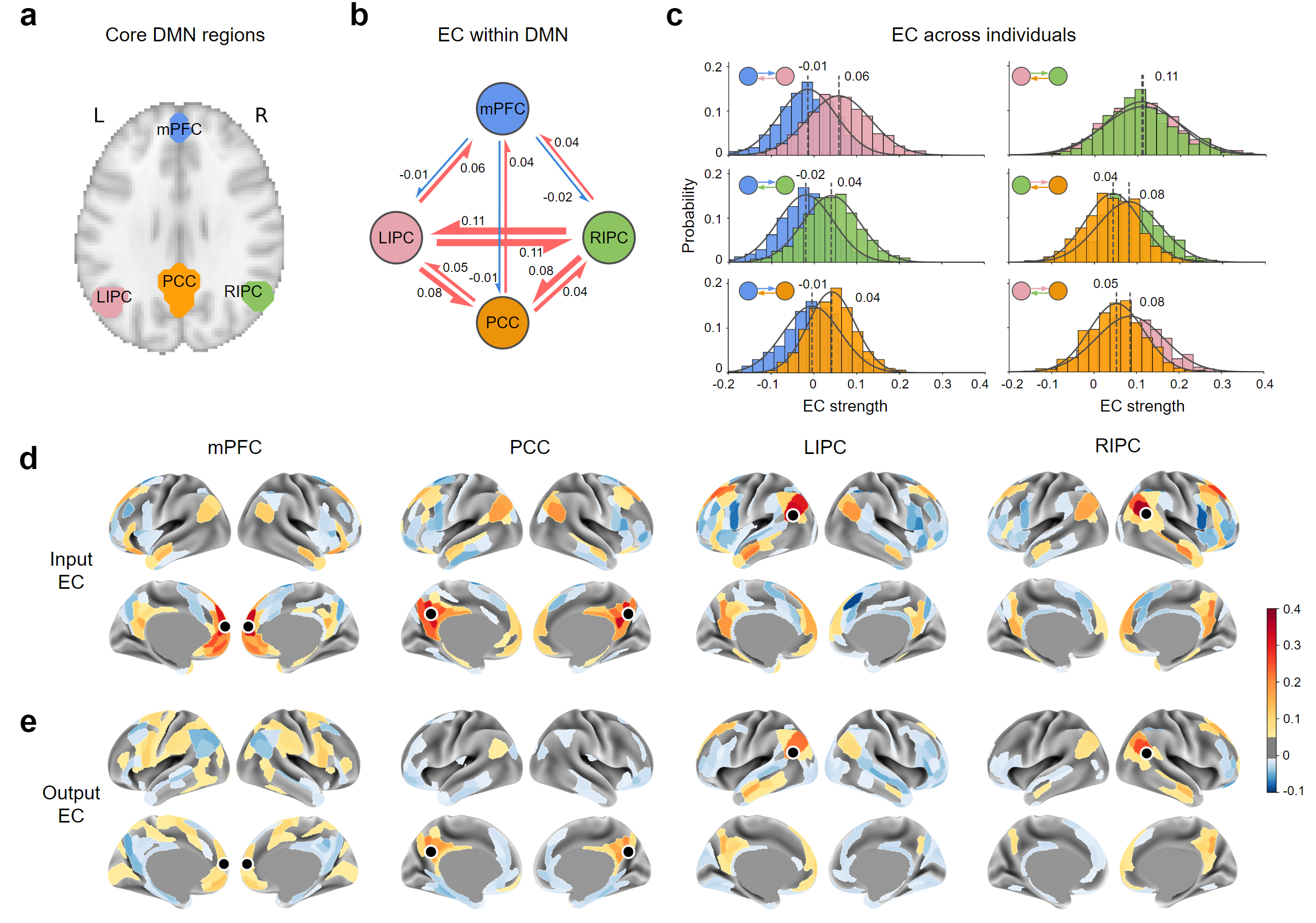
Figure 5: Information flow within DMN and between DMN and cortex (a) The core DMN regions include the medial prefrontal cortex (mPFC), left inferior parietal cortex (LIPC), right inferior parietal cortex (RIPC), and posterior cingulate cortex (PCC). (b) The EC among core DMN regions is depicted, with excitatory EC represented in red and inhibitory EC represented in blue. The thickness of the arrows reflects the strength of the EC. (c) The distribution of the strengths of EC within DMN across subjects. The distribution is colored as the color of the source regions. Twelve ECs within DMN are all significantly existing ($p\leq 0.05$, FDR corrected). (d,e) The input (d) and output (e) EC between the core DMN regions and the cortex are depicted on a topographical map.

DMN is a functional network that is generally more active during rest or spontaneous thought than during task performing. It is thought to be involved in a wide range of cognition, such as memory consolidation, social cognition, and the integration of information from different brain regions Raichle2015Brain ; Christoff2016Mindwandering ; Margulies2016Situating . However, the mechanisms by which the DMN performs these functions are elusive, particularly in terms of macroscopic information integration. Our inferred EBC reveals that DMN has the highest inter-network inhibitory density (Fig. 4h), thus playing an inhibitory role in cortical dynamics. We examine the information flows within and across DMN and focuse on the four core regions of the DMN: the medial prefrontal cortex (mPFC), left inferior parietal cortex (LIPC), right inferior parietal cortex (RIPC), and posterior cingulate cortex (PCC) (Fig. 5a).

Since the MMP atlas does not explicitly contain all four core DMN regions, the BOLD signals from core DMN regions are separately extracted (Table  S3) and combined with 379-dimensional signals from MMP, yielding 383-dimensional signals. The NPI applied to the 383-dimensional signals to get the EC within and across DMN. The inferred EC within the core DMN regions and their inter-individual variability are shown in Fig. 5b,c. All twelve ECs among core DMN regions are significantly existing. There are weak inhibitory ECs from mPFC to the other three regions, suggesting an inhibitory role of mPFC within the DMN. All other ECs within core DMN are excitatory.

The DMN’s inflow from the cortex and its outflow to the cortex are shown in Fig. 5d,e. Although there are overlaps between the corresponding inflow and outflow, they are not identical. Despite the inhibitory ECs from mPFC to other three DMN regions, mPFC outputs excitatory ECs to a wide range of cortical regions, suggesting the role of the mPFC in integrating information from the DMN and spreading to other parts of the cortex, which is possibly linked to memory consolidation and consciousness formation Euston2012Role ; Mashour2020Conscious .

2.6 EBC explains SC and FC

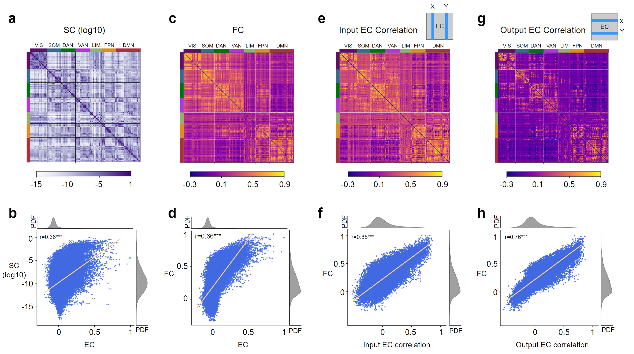
Figure 6: The structural, functional, and effective connectome of human brain (a) The SC of the left hemisphere is obtained from diffusion tensor imaging (DTI) data and averaged across 800 subjects. (b) The correlation between the strength of the same connections in SC and EC ($r=0.36$, $p<10^{-4}$). (c) The FC of the left hemisphere for 800 subjects is calculated as Pearson’s correlation coefficient of fMRI signals among cortical regions. (d) The correlation between the strength of the same connections in FC and EC ($r=0.66$, $p<10^{-4}$). (e) We define the input EC correlation of the region $X$ and $Y$ as the correlation between the $X$-$th$ and the $Y$-$th$ column of EBC, which measures the similarity of inputs to region $X$ and region $Y$. (f) The correlation between the strength of the FC input EC correlation ($r=0.85$, $p<10^{-4}$). (g) We define the output EC correlation of the region $X$ and $Y$ as the correlation between the $X$-$th$ and the $Y$-$th$ row of EBC, which measures the similarity of outputs from region $X$ and region $Y$. (h) The correlation between the strength of the FC and output EC correlation ($r=0.76$, $p<10^{-4}$).

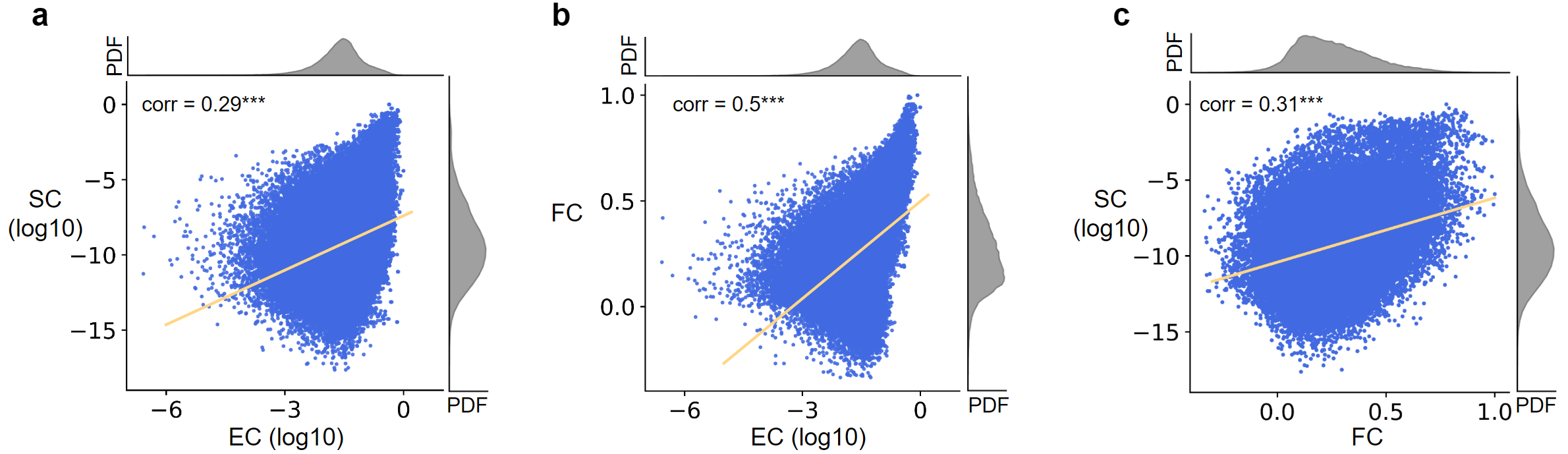
Figure S13: The relationship among SC, FC, and log-transformed EC (a,b) The log-transformed EC strengths are strongly correlated with log-transformed SC ($r=0.29,p\leq 10^{-4}$) and FC ($r=0.50,p\leq 10^{-4}$). (c) The FC strengths are strongly correlated with log-transformed SC ($r=0.31,p\leq 10^{-4}$).

To better understand how brain structure supports its rich functionality, we examine the relationship among whole-brain SC, EC, and FC. We find that EC is strongly correlated with both SC and FC, and all three connectomes demonstrate a modular structure with higher connections within functional networks (Fig. 6a-d). The correlation between EC and SC is higher than that between FC and SC, indicating that EC better explains SC than FC (Fig. 6b, Fig. S13c). For a strong EC, there is usually a strong SC, suggesting the SC provides a structural basis for effective information flow.

FC has widely been used to understand the important inter-regional interactions in diseases, cognitive tasks, and behaviors. However, the incomplete understanding of the formation mechanism of FC limits the study of the neural basis underlying FC differences. Most connections in SC and EC have very small strengths, while FC has a larger average strength, which may result from spurious connections caused by confounds (Fig. 6d). The entries with strong EC tend to have strong FC, while entries with small EC can have either strong or weak FC (Fig. 6d), which also indicates vast indirect connections and confounds in FC.

To measure the role of indirect EC in the formation of FC, we examine the similarity of input and output EC of every pair of regions and see how they relate to FC. The input EC correlation between regions $X$ and $Y$ is calculated as the correlation between the $X$-$th$ column and the $Y$-$th$ column of the EBC (Fig. 6e). A high input EC correlation indicates that two regions have many shared inputs, which may contribute to enhanced FC between them. Similarly, output EC correlation between regions $X$ and $Y$ is calculated as the correlation between the $X$-$th$ row and the $Y$-$th$ row of the EBC (Fig. 6g). A high output EC correlation suggests that two regions have many shared outputs. Our results showed that input EC correlation is a better predictor of FC than output EC correlation and EC itself (Fig. 6f,h), suggesting that FC is determined by both direct connections and shared inputs.

3 Discussion

Our brain is a distributed and interactive network that allows for receiving stimulus inputs and generating response outputs Telesford2011Brain ; ThiebautdeSchotten2022emergent . Understanding this input-output causal relationship among the entire brain requires mapping the EBC. In this study, we presented a data-driven framework called NPI to infer the EBC with directionality, strength, and excitatory-inhibitory distinction of causal relationships. We applied NPI to resting-state human fMRI data and obtained the human EBC, which uncovered the whole-brain organization of excitatory and inhibitory ECs within and across functional networks.

3.1 NPI is a general data-driven framework to infer causal relationship

Despite EC as a common terminology in the neuroscience literature Friston2014DCM ; Barnett2014MVGC ; Singh2020Estimation , the definition of EC is ambiguous: its meaning and connotation vary across different methods. For example, EC from region $X$ to region $Y$ in the context of Granger causality refers to the importance of the history of $X$ in predicting the activity of $Y$, while EC in DCM is defined as the coupling parameters in a mechanistic state-space model. There is an ongoing debate about how these definitions relate to the underlying flow of information in the brain. In this study, we define EC as the magnitude of the neural response induced by a perturbation to a specific brain region. This definition aligns with the statistical definition of causality: $X$ has a causal effect on $Y$ if an externally applied perturbation of $X$ can result in a significant change in $Y$ Pearl2009Causality ; Woodward2016Causation . This definition is well consistent with the experimental methods that infer EC by actually perturbing a region and observing the remote neural response, which is believed to recruit the underlying physical connections and reflect the information flow in the brain.

The performance EC inference relies on the ability of ANN in predicting the neural response after applying perturbations. After training ANN through one-step-ahead prediction, it successfully learned the mapping between two consecutive signals in both simulated dataset and real BOLD signals. More importantly, the trained ANN generalize to the perturbed unseen input (out-of-distribution samples) (Fig. 2g). This excellent fitting ability comes from the great expressive power of over-parameterized ANN models, which has been extensively studied in the field of deep learning Neyshabur2019ROLE ; Zhang2021Understanding . Therefore, the perturbation-induced signal change predicted by ANN is believed to be equivalent to the signal change in the real brain with similar a stimulation. In the future, the prediction ability of ANN can be validated using concurrent stimulation and observation such as concurrent TMS-fMRI.

Predicting the next state using only the current state requires the system to be nearly Markovian. In fMRI signals, the time repeat is usually large, so that the current fMRI state contains nearly all the information needed to predict the next state, suggesting that fMRI signals are almost Markovian Nozari2021brain . Thus, the present BOLD signal is sufficient to predict one-step-ahead BOLD response. The prediction of EEG data may require many history steps, as the time length of one step is much smaller in EEG Nozari2021brain . To adapt NPI for other data modalities, such as EEG data, the ANN architecture and the way applying perturbation may need be adjusted to utilize past information in more time steps.

The NPI framework inherits a major limitation of data-driven methods: it is data-hungry (Fig.2j). Since the small models usually have limited ability in data fitting and generalization, an ANN with a large number of parameters is needed to ensure great generalization ability, which is the key to an accurate inference. However, a large model also needs more data to be trained. It is necessary to find a trade-off in the model size, where it has enough expression ability and can be trained with a moderate amount of data. The inference method that needs fewer data is a future direction. While the MLP used in this study is one option for the prediction model, any model that is able to accurately describe the underlying brain network dynamics could potentially be used in the NPI framework Liang2022Online ; Koppe2019Identifying . Prediction models with better data efficiency are in need. On the other hand, more prior knowledge in neuroscience may be incorporated to build surrogate models with fewer parameters and thus needs less data.

3.2 Insights from the human resting-state EBC

Macroscopic information flow plays a crucial role in processing sensory inputs and mediating cognitive functions, such as attention, memory, and behaviors. This information flow involves both feedforward processing and feedback signaling, with sensory information being transmitted to and further processed by higher-level brain regions before flowing back Semedo2022Feedforward ; Mejias2016Feedforward . Multimodal feedforward and feedback information flow and higher-level information integration occur in parallel. The NPI-inferred EBC provides a complete picture of this parallel information flow in the brain. In human EBC, the strength of ECs followed a log-normal distribution for both excitatory and inhibitory ECs, indicating most ECs are weak, with only a few being strong. It is consistent with the distribution of SC in many species, as EC is constrained by SC Oh2014mesoscale ; Markov2014Weighted . In network science, this log-normal distribution is considered as the result of a trade-off between minimizing wiring costs and energy consumption while maintaining efficient inter-regional communication Ercsey-Ravasz2013Predictive .

The EBC has the merit of discrimination between excitatory and inhibitory ECs between brain regions. Our results show that the majority of ECs in the EBC are excitatory, which have a larger maximum strength and averaged strength compared with inhibitory ECs. Additionally, the spatial distribution of excitatory and inhibitory ECs vary, with excitatory ECs being concentrated in local communities such as within functional networks and within a hemisphere, while inhibitory ECs had a higher averaged strength across communities. The averaged strengths of ECs within and across functional networks also vary, where excitatory ECs have a higher averaged strength within unimodal networks such as the visual and somatomotor networks, and inhibitory ECs have a higher averaged strength within transmodal networks, particularly within the frontoparietal and default mode networks. Moreover, the hierarchy of averaged excitatory and inhibitory connection strengths is similar to the large-scale cortical hierarchy from unimodal networks that process information from a single modality such as visual and motor networks to transmodal networks that integrate information from various sources such as the DMN Huntenburg2018Large-Scale . It suggests that unimodal networks require extensive excitatory ECs to recurrently process primary information within the networks. Transmodal networks, on the contrary, need inhibitory ECs to modulate and integrate information across various networks Sanzeni2020Inhibition ; Kim2021Strong ; Mongillo2018Inhibitory .

DMN is located at one end of the cortical hierarchy and is known to process transmodal information unrelated to immediate sensory inputs Margulies2016Situating ; Christoff2016Mindwandering . How DMN receive information from and transmit information to other cortical regions are unclear. Our results show the EC within the core DMN regions with excitatory-inhibitory distinction, where the result is similar to previous DCM-based findings in some way Almgren2018Variability . The mPFC receives excitatory ECs from other three regions in DMN, but output inhibitory ECs to all of them. On the other hand, mPFC has a wide range of excitatory ECs to the cortex, suggesting the role of mPFC in integrating information from other DMN regions and broadcasting to a wide range of cortex, which is in line with the role of global broadcasting of information suggested in the global neuronal workspace theory of consciousness formation Euston2012Role ; Mashour2020Conscious .

3.3 The relationship among SC, FC, and EBC

How static brain structure supports rich brain functionality is a central question in neuroscience. However, the structure-function relationship at the macroscopic scale remains poorly understood due to the difficulties in observation with a high spatiotemporal scale and the lack of suitable tools for EC inference. Traditional measures of brain networks, including SC and FC, are insufficient to describe the property that we are interested in: the actual inter-region interactions, which should ideally be a causal interaction with directionality, strength, and excitatory-inhibitory distinction. So far, the SC derived from MRI could not capture the directionality of connections nor distinguish the excitatory or inhibitory connections Yeh2021Mapping . The FC derived from statistical correlation still does not describe information flow in the brain, since correlation is affected by input signals from other nearby regions and does not reflect the directionality of connections Cole2014Intrinsic ; Hearne2021Activity .

NPI-inferred EC represents how one brain region causally influences another. This influence is a compositive effect that depends not only on SC but also on brain dynamics and regional heterogeneity. After a perturbation, the response is expected to propagate along physical connections (SC), while the magnitude of the propagated response is modulated by the nonlinear brain dynamics, as well as the current brain state. The interpretation of NPI-inferred EC replies on the specific temporal and spatial scale of observed data, as the EC at a large spatiotemporal scale can be the integration of finer-scale connections. The regions at a large spatial scale can actually contain many sub-populations, with excitatory and inhibitory ECs among sub-populations. The EC between two large regions is thus a composite effect after the cancellation of excitatory and inhibitory ECs among sub-populations. On a large temporal scale, the EC can be the composite effect of indirect information flow that passed other regions at a finer timescale. Therefore, EC should be considered at a specific spatiotemporal scale as it changes with the scales of observation. In the NPI framework, the ANN learns brain dynamics from neural signals. The EC obtained by perturbing ANN is thus the EC at the spatiotemporal scale that the neural signals are sampled. For the RNN model, we observed the signals at the finest spatial scale and also a small timescale. The EC is thus highly correlated with SC. The EBC inferred from BOLD signals, on the other hand, represents the EC at a large spatiotemporal scale which may integrate the effects of underlying SC, excitatory-inhibitory balance, neural dynamics, hemodynamics, and regional heterogeneity. Despite that, the obtained EBC is strongly correlated with whole-brain SC, suggesting the shared network topology in brain structure and function. A potential future direction is to investigate how SC and macroscopic brain dynamics interact to support EC.

Like EC, FC is also a composite effect that integrates various factors, but it does not reflect a directed influence. We calculate the input EC correlation and output EC correlation and find that the input EC correlation better explains FC than EC itself. This deepens the interpretation of the FC network and suggests FC is the result of both similar EC inputs and direct EC. This motivates us to advance our concentration from FC to EC when studying functional interactions.

3.4 Future applications of NPI framework

Although we apply NPI to resting-state fMRI data in this study, NPI is a versatile framework. Adjusting the ANN architecture and the paradigm of virtual perturbation allows adapting NPI to various data modalities with multiple spatiotemporal scales. For example, NPI can be applied to neural data spanning from individual neurons to neural populations and large-scale EEG and fMRI. Integrating EC across multiple scales could potentially deepen our understanding of structure-function relationships and reveal the mechanisms through which high-level intelligence emerges from multi-scale connections, offering a more comprehensive understanding of brain function. Besides neural signals, NPI also has the potential to be extended to other types of data, such as traffic flow and social network data, as long as they can be represented as time series.

In clinical applications, NPI has the potential to uncover biomarkers for neurological diseases and guide the target selection in neurostimulation. Applying NPI to the neural signals of patients with neurological diseases can reveal the patients’ EBC. Comparing the EBC of patients and healthy people helps in identifying reorganizations of information flow in the disease and providing mechanical biomarkers. As neural stimulation is transmitted along the information flow, NPI also aids in the selection of control nodes for personalized neurostimulation. Neurostimulation to specific brain regions has been increasingly used to treat brain diseases, such as subthalamic nucleus for Parkinson’s disease Schuepbach2013Neurostimulation and ventral capsule/ventral striatum (VC/VS) region for depression Scangos2021Closedloop . The desired control node in specific neural disorders is often located in deep brain regions, which are hard to access for direct stimulation. In clinical practice, regions on the brain surface are often chosen as control regions to indirectly influence target regions in the deep brain. However, due to inter-individual differences in brain connectivity, selecting the optimal control region remains a challenge. NPI provides personalized EC and is thus useful in guiding the selection of the stimulation region. NPI also serves as a framework to test the effect of different neurostimulation paradigms. For the purpose of EC inference, we only perturbed one node at a time. Real neurostimulation may achieve a better performance when stimulating multiple brain regions at a time. NPI offers a convenient framework for predicting the effect of multi-region perturbation, as well as the effect of repeated stimulation and stimulation response under different brain states.

4 Methods

4.1 The NPI framework

The NPI framework consists of two steps: i) training an ANN to predict the whole-brain neural dynamics as a surrogate brain, and ii) applying perturbations to each input node of the trained ANN as virtual neurostimulation to brain regions.

First, an ANN $f(\cdot)$ is applied to model the regional neural dynamics,

$$\hat{\mathbf{x}}_{t+1}=f(\mathbf{x}_{t},\theta),$$

where $\theta$ is the vector of all unknown parameters in the ANN model. $\mathbf{x}_{t}$ is the vectorized fMRI data across the cortical areas at time step $t$, and $\hat{\mathbf{x}}_{t+1}$ is the predicted fMRI data at time step $t+1$ by the ANN model. Notably, the ANN can be realized with a variety of network architectures as long as it has the sufficient expressive power to fit the whole-brain neural dynamics. In this study, we use a multi-layer perceptron (MLP) architecture to realize the ANN model. The number of units in the first layer and the last layer of ANN is set to the number of brain regions. The number of units in hidden layers can vary with the complexity of the neural data applied for inferring EC. In this study, a five-layer MLP with the number of units $379,800,1000,1000,800,379$, and the $ReLU$ activation function is used.

The ANN model is trained by minimizing the one-step-ahead prediction error (predicting the BOLD signal at the next time step given the signal at the current time step). The fMRI data are organized as pairs of two consecutive time points, $\mathbf{x}_{t}$ and $\mathbf{x}_{t+1}$. The objective function $\mathcal{L}(\theta)$ can be explicitly formulated as:

$$\mathcal{L}(\theta)=\|f(\mathbf{x}_{t},\theta)-\mathbf{x}_{t+1}\|.$$

The Adam optimizer is used to learn the network parameter $\theta$.

The ANN model is trained separately for each subject using all four sessions of rsfMRI data. The data from each sessions are divided into numerous input-output pairs, where the input the signal at a particular time point and the output is the signal at the next time point. The training pairs from all four sessions are combined, and 5% of these pairs are randomly extracted as the testing set for that specific subject.

Once the ANN is trained, we perform virtual perturbations to each input node of ANN to infer the EC of brain regions. The perturbation is implemented as a selective increase of the BOLD signal at one specific region. By observing the induced response at all other regions, the one-to-all EC is inferred. The EC from the region $A$ to the region $B$ can thus be expressed as:

$$\delta_{A\to B}=\mathbb{E}[(B_{t+1}\mid A_{t}=A_{t}+\Delta)-(B_{t+1}\mid A_{t}=A_{t})],$$

where $\Delta$ is the strength of perturbation that is applied to the region $A$. The mapping from the signal at time $t$ to the signal at time $t+1$ is realized by the trained ANN model. The perturbation is only perturbed to one region at a time, where the signals of all other regions remain the same. When applying to the real BOLD signal, we set $\Delta$ as half of the standard deviation of the BOLD activity. We also test different perturbation strengths and find the inference performance is robust to the perturbation strength.

4.2 Synthetic data from RNN model

To validate the performance of NPI, we generate synthetic data using RNN models with fixed ground-truth SC. We denote the state of the $i$th neuron as $x_{i}$ and $x=(x_{1},...x_{n})$ is a $n$-dimensional vector that represents the states of all the $n$ neurons in the network. The dynamics of $x$ are given by the following equation:

$$\frac{d}{dt}x=-x+Wh(x)+\sigma v$$

where $W$ is the connectivity matrix (SC) and $h()$ is the $\tanh$ activation function. The entries of the weight matrix $W$ are independent identically distributed centered Gaussians $\mathcal{N}(0,n^{-1/2})$. The initial state is sampled from a Gaussian distribution $\mathcal{N}(0,1)$. The $\sigma$ is the standard deviation of a Gaussian noise $v\sim\mathcal{N}(0,1)$. The neural dynamics are simulated with the Euler method where $dt=0.01$.

The perturbations applied to the model are implemented in the same way in NPI. Only the signal of the source region is increased by a particular value, while the signal of all other regions remains the same compared with the unperturbed state.

When testing the prediction ability of ANN, the input-output pairs in training data is constructed by consecutive pairs of the generated neural signals. The input in the test dataset is constructed by applying a perturbation to signals randomly chosen from the generated neural signals. The corresponding output is then mapped by the RNN dynamics. These inputs in the test dataset are out-of-distribution samples that are not in the distribution of the training data, which are consistent with the situation for applying NPI to the real BOLD signals.

4.3 Empirical data and the brain atlas

Human Connectome Project (HCP) S1200 release VanEssen2013WU-Minn which includes resting-state fMRI (rs-fMRI) data from 800 subjects is used in this study. The preprocessing of fMRI is based on the multi-modal inter-subject registration (MSMAII) Robinson2014MSM . The rsfMRI data is recorded with TR 0.72s. Each subject comprises two sessions on separate days and each day contains two runs of 15-min rsfMRI, resulting in four runs in total. Every consecutive time point is organized as input-output pairs. The pairs for four runs are mixed to train the model. When testing prediction performance, the testing set comprises 5% randomly sampled pairs in all shuffled input-output pairs and the rest data are used to train the model.

The brain is parcellated into 379 regions according to the Multi-Modal Parcellation atlas (MMP 1.0) Glasser2016multi-modal , consisting of 180 cortical regions in each hemisphere and 19 subcortical regions. The analysis is based on the EC among 360 cortical regions, where subcortical regions are included in the training to reduce the bias of EC inference from unobserved regions. The parcellation is performed by averaging the BOLD signals across voxels in each cortical region. To validate the robustness of the NPI framework in inferring EC across spatial scales of parcellations, we replicate the EBC results with the AAL atlas, a parcellation with 116 regions Tzourio-Mazoyer2002Automated .

4.4 Construction of the whole-brain SC, FC, and EC

The resting-state fMRI time series is preprocessed according to the HCP minimal preprocessing pipeline glasser2013minimal . The denoising process is performed using ICA-FIX which cleans the structured noise by a process combining independent component analysis and the FSL tool FIX. The denoised data are further processed using the Python package nilearn Abraham2014Machine that extracts the data at 0.1 to 0.01 Hz. FC is calculated as Pearson’s correlation coefficient between the time series of each pair of brain regions. The FC of one subject is obtained by averaging the FC of four runs.

The structural connectivity constructed by Demirtaş et al. Demirtas2019Hierarchical is used. It is derived using FSL’s bedpostx and probtrackx2 analysis workflows that count the number of streamlines intersecting the white matter and gray matter. The SC matrix is scaled to range from $0$ to $1$ and then log-transformed. The EC for each subject is obtained from the NPI framework that is trained using the four runs of fMRI of each subject. It is then averaged across 800 subjects and scaled as the strongest connection has strength one.

4.5 Parcellation of functional networks

The parcellated 360 cortical regions are assigned to seven functional networks, according to the resting-state networks defined in Yeo et al. ThomasYeo2011organization . The seven functional networks are the visual network (VIS), the somatomotor network (SOM), the dorsal attention network (DAN), the ventral attention network (VAN), the frontoparietal control network (FPN), and the default mode network (DMN). Each region is assigned to the functional network with the largest number of voxels to that region belongs. We place the seed in the left-hemisphere core brain region of each of the seven functional networks (seeds are shown in Table S2). Then we calculate the seed-based FC using Pearson’s correlation between the seed region and the rest regions.

4.6 EC between DMN and other cortical regions

We analyze the EC within core regions in DMN and EC between a region in DMN and the rest of the brain regions. Since the MMP atlas does not contain all the core DMN regions, we extract the BOLD signals in four DMN regions according to MSDL parcellation Varoquaux2011Multi-subject : mPFC, LIPC, RIPC, and PCC, with coordinates in Table S3. These four signals are combined with the BOLD signals from the MMP parcellation of 379 cortical regions, resulting in the signal with 383 regions. The ANN is then trained on the combined signals. After the model training, the EC within DMN and the EC between DMN and other regions are extracted for further investigations.

Acknowledgments This work is supported by the National Natural Science Foundation of China (62001205), National Key R&D Program of China (2021YFF1200804), Shenzhen Science and Technology Innovation Committee (20200925155957004, KCXFZ2020122117340001, SGDX2020110309280100), Shenzhen Key Laboratory of Smart Healthcare Engineering (ZDSYS20200811144003009), Guangdong Provincial Key Laboratory of Advanced Biomaterials (2022B1212010003). We thank Prof. Changfeng Wu, Prof. Jing Jiang, Prof. Kai Du, Prof. Yu Mu, Prof. Dayong Jin, Prof. Haiyan Wu, Chen Wei, Shengyuan Cai, Kaining Peng, and Xin Xu for stimulating discussions and advice.

Supplementary materials

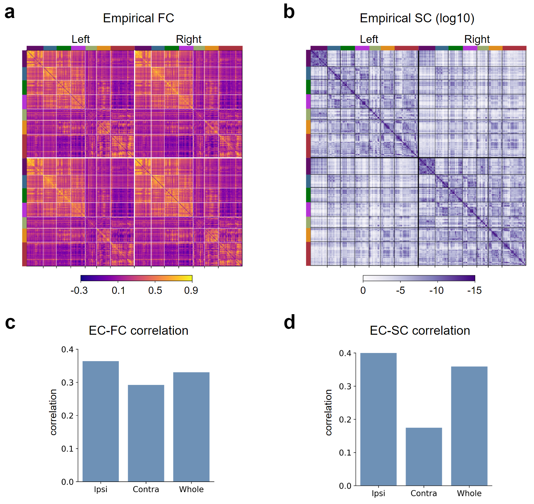
Figure S14: The whole-brain FC and SC and their correlation with EC. (a, b) The whole-brain FC (a) and SC (b). (c,d) Correlation between FC (c), SC (d) and EC for ipsi-lateral connections, contra-lateral connections, and whole-brain connections.

Table S1: AIC of fitting the distribution of EBC strengths

Distribution	Excitatory EC	Inhibitory EC	Absolute EC
Log-normal	773	4	832
Inverse-Gaussian	956	41	1076
Exponential	2111	164	2592
Normal	11256	1621	14598

Table S2: MNI Coordinates of seed regions in the brain functional networks

Network	Seed region	MNI Coordinate
VIS	L V2	(-12.72, -81.95, 1.04)
SOM	L 3b	(-41.40, -21.76, 50.97)
VAN	L VIP	(-37.76, -44.82, 42.39)
DAN	L FOP3	(-37.44, 2.97, 12.33)
FPN	L a9-46v	(-40.90, 49.90, 8.64)
DMN	L TE1a	(-63.78, -11.05, -22.60)

Table S3: MNI Coordinates of core DMN regions

DMN region	MNI Coordinate
mPFC	(-0.15, 51.42, 7.58)
LIPC	(-45.8, -64.78, 31.84)
RIPC	(51.66, -59.34, 28.88)
PCC	(-0.2, -55.21, 29.87)

References

- \bibcommenthead
- (1) Park, H.-J. & Friston, K. Structural and functional brain networks: From connections to cognition. Science 342 (6158), 1238411 (2013). 10.1126/science.1238411 .
- (2) Yeh, C.-H., Jones, D. K., Liang, X., Descoteaux, M. & Connelly, A. Mapping structural connectivity using diffusion mri : Challenges and opportunities. Journal of Magnetic Resonance Imaging 53 (6), 1666–1682 (2021). 10.1002/jmri.27188 .
- (3) van den Heuvel, M. P. & Hulshoff Pol, H. E. Exploring the brain network: A review on resting-state fmri functional connectivity. European Neuropsychopharmacology 20 (8), 519–534 (2010). 10.1016/j.euroneuro.2010.03.008 .
- (4) Schippers, M. B., Roebroeck, A., Renken, R., Nanetti, L. & Keysers, C. Mapping the information flow from one brain to another during gestural communication. Proceedings of the National Academy of Sciences 107 (20), 9388–9393 (2010). 10.1073/pnas.1001791107 .
- (5) Pearl, J. Causality (Cambridge University Press, 2009).
- (6) Veit, M. J. et al. Temporal order of signal propagation within and across intrinsic brain networks. Proceedings of the National Academy of Sciences 118 (48), e2105031118 (2021). 10.1073/pnas.2105031118 .
- (7) Ozdemir, R. A. et al. Individualized perturbation of the human connectome reveals reproducible biomarkers of network dynamics relevant to cognition. Proceedings of the National Academy of Sciences 117 (14), 8115–8125 (2020). 10.1073/pnas.1911240117 .
- (8) Keller, C. J. et al. Mapping human brain networks with cortico-cortical evoked potentials. Philosophical Transactions of the Royal Society B: Biological Sciences 369 (1653), 20130528 (2014). 10.1098/rstb.2013.0528 .
- (9) Bauer, A. Q. et al. Effective connectivity measured using optogenetically evoked hemodynamic signals exhibits topography distinct from resting state functional connectivity in the mouse. Cerebral Cortex 28 (1), 370–386 (2018). 10.1093/cercor/bhx298 .
- (10) Friston, K. J., Kahan, J., Biswal, B. & Razi, A. A dcm for resting state fmri. NeuroImage 94, 396–407 (2014). 10.1016/j.neuroimage.2013.12.009 .
- (11) Barnett, L. & Seth, A. K. The mvgc multivariate granger causality toolbox: A new approach to granger-causal inference. Journal of Neuroscience Methods 223, 50–68 (2014). 10.1016/j.jneumeth.2013.10.018 .
- (12) Li, S., Xiao, Y., Zhou, D. & Cai, D. Causal inference in nonlinear systems: Granger causality versus time-delayed mutual information. PHYSICAL REVIEW E 9 (2018) .
- (13) Lundervold, A. S. & Lundervold, A. An overview of deep learning in medical imaging focusing on mri. Zeitschrift für Medizinische Physik 29 (2), 102–127 (2019). 10.1016/j.zemedi.2018.11.002 .
- (14) Pandarinath, C. et al. Inferring single-trial neural population dynamics using sequential auto-encoders. Nature Methods 15 (10), 805–815 (2018). 10.1038/s41592-018-0109-9 .
- (15) Yan, Y. et al. Reconstructing lost bold signal in individual participants using deep machine learning. Nature Communications 11 (1), 5046 (2020). 10.1038/s41467-020-18823-9 .
- (16) Liang, Z., Luo, Z., Liu, K., Qiu, J. & Liu, Q. Online learning koopman operator for closed-loop electrical neurostimulation in epilepsy. IEEE Journal of Biomedical and Health Informatics 1–12 (2022). 10.1109/JBHI.2022.3210303 .
- (17) Kim, J. Z., Lu, Z., Nozari, E., Pappas, G. J. & Bassett, D. S. Teaching recurrent neural networks to infer global temporal structure from local examples. Nature Machine Intelligence 3 (4), 316–323 (2021). 10.1038/s42256-021-00321-2 .
- (18) Samek, W., Montavon, G., Lapuschkin, S., Anders, C. J. & Muller, K.-R. Explaining deep neural networks and beyond: A review of methods and applications. Proceedings of the IEEE 109 (3), 247–278 (2021). 10.1109/JPROC.2021.3060483 .
- (19) Van Essen, D. C. et al. The wu-minn human connectome project: An overview. NeuroImage 80, 62–79 (2013). 10.1016/j.neuroimage.2013.05.041 .
- (20) Scangos, K. W., Makhoul, G. S., Sugrue, L. P., Chang, E. F. & Krystal, A. D. State-dependent responses to intracranial brain stimulation in a patient with depression. Nature Medicine 27 (2), 229–231 (2021). 10.1038/s41591-020-01175-8 .
- (21) Sanchez-Romero, R. et al. Estimating feedforward and feedback effective connections from fmri time series: Assessments of statistical methods. Network Neuroscience 3 (2), 274–306 (2019). 10.1162/netn_a_00061 .
- (22) Thomas Yeo, B. T. et al. The organization of the human cerebral cortex estimated by intrinsic functional connectivity. Journal of Neurophysiology 106 (3), 1125–1165 (2011). 10.1152/jn.00338.2011 .
- (23) Oh, S. W., Harris, J. A., Ng, L. & Winslow, B. A mesoscale connectome of the mouse brain. Nature 21 (2014) .
- (24) Markov, N. T. et al. A weighted and directed interareal connectivity matrix for macaque cerebral cortex. Cerebral Cortex 24 (1), 17–36 (2014). 10.1093/cercor/bhs270 .
- (25) Felleman, D. J. & Van Essen, D. C. Distributed hierarchical processing in the primate cerebral cortex. Cerebral Cortex 1 (1), 1–47 (1991). 10.1093/cercor/1.1.1 .
- (26) Margulies, D. S. et al. Situating the default-mode network along a principal gradient of macroscale cortical organization. Proceedings of the National Academy of Sciences 113 (44), 12574–12579 (2016). 10.1073/pnas.1608282113 .
- (27) Murray, J. D. et al. A hierarchy of intrinsic timescales across primate cortex. Nature Neuroscience 17 (12), 1661–1663 (2014). 10.1038/nn.3862 .
- (28) Raichle, M. E. The brain’s default mode network. Annual Review of Neuroscience 38 (1), 433–447 (2015). 10.1146/annurev-neuro-071013-014030 .
- (29) Christoff, K., Irving, Z. C., Fox, K. C. R., Spreng, R. N. & Andrews-Hanna, J. R. Mind-wandering as spontaneous thought: A dynamic framework. Nature Reviews Neuroscience 17 (11), 718–731 (2016). 10.1038/nrn.2016.113 .
- (30) Euston, D. R., Gruber, A. J. & McNaughton, B. L. The role of medial prefrontal cortex in memory and decision making. Neuron 76 (6), 1057–1070 (2012). 10.1016/j.neuron.2012.12.002 .
- (31) Mashour, G. A., Roelfsema, P., Changeux, J.-P. & Dehaene, S. Conscious processing and the global neuronal workspace hypothesis. Neuron 105 (5), 776–798 (2020). 10.1016/j.neuron.2020.01.026 .
- (32) Telesford, Q. K., Simpson, S. L., Burdette, J. H., Hayasaka, S. & Laurienti, P. J. The brain as a complex system: Using network science as a tool for understanding the brain. Brain Connectivity 1 (4), 295–308 (2011). 10.1089/brain.2011.0055 .
- (33) Thiebaut de Schotten, M. & Forkel, S. J. The emergent properties of the connected brain. Science 378 (6619), 505–510 (2022). 10.1126/science.abq2591 .
- (34) Singh, M. F., Braver, T. S., Cole, M. W. & Ching, S. Estimation and validation of individualized dynamic brain models with resting state fmri. NeuroImage 221, 117046 (2020). 10.1016/j.neuroimage.2020.117046 .
- (35) Woodward, J. in Causation and manipulability Winter 2016 edn, (ed.Zalta, E. N.) The Stanford Encyclopedia of Philosophy (Metaphysics Research Lab, Stanford University, 2016).
- (36) Neyshabur, B., Li, Z. & Bhojanapalli, S. The role of over-parametrization in generalization of neural networks (2019) .
- (37) Zhang, C., Bengio, S., Hardt, M., Recht, B. & Vinyals, O. Understanding deep learning (still) requires rethinking generalization. Communications of the ACM 64 (3), 107–115 (2021). 10.1145/3446776 .
- (38) Nozari, E. et al. Is the brain macroscopically linear? a system identification of resting state dynamics (2021). arXiv:2012.12351.
- (39) Koppe, G., Toutounji, H., Kirsch, P., Lis, S. & Durstewitz, D. Identifying nonlinear dynamical systems via generative recurrent neural networks with applications to fmri. PLOS Computational Biology 15 (8), e1007263 (2019). 10.1371/journal.pcbi.1007263 .
- (40) Semedo, J. D. et al. Feedforward and feedback interactions between visual cortical areas use different population activity patterns. Nature Communications 13 (1), 1099 (2022). 10.1038/s41467-022-28552-w .
- (41) Mejias, J. F., Murray, J. D., Kennedy, H. & Wang, X.-J. Feedforward and feedback frequency-dependent interactions in a large-scale laminar network of the primate cortex. SCIENCE ADVANCES (2016) .
- (42) Ercsey-Ravasz, M. A predictive network model of cerebral cortical connectivity based on a distance rule. Neuron 14 (2013) .
- (43) Huntenburg, J. M., Bazin, P.-L. & Margulies, D. S. Large-scale gradients in human cortical organization. Trends in Cognitive Sciences 22 (1), 21–31 (2018). 10.1016/j.tics.2017.11.002 .
- (44) Sanzeni, A. et al. Inhibition stabilization is a widespread property of cortical networks. eLife 9, e54875 (2020). 10.7554/eLife.54875 .
- (45) Kim, R. & Sejnowski, T. J. Strong inhibitory signaling underlies stable temporal dynamics and working memory in spiking neural networks. Nature Neuroscience 24 (1), 129–139 (2021). 10.1038/s41593-020-00753-w .
- (46) Mongillo, G., Rumpel, S. & Loewenstein, Y. Inhibitory connectivity defines the realm of excitatory plasticity. Nature Neuroscience 21 (10), 1463–1470 (2018). 10.1038/s41593-018-0226-x .
- (47) Almgren, H. et al. Variability and reliability of effective connectivity within the core default mode network: A multi-site longitudinal spectral dcm study. NeuroImage 183, 757–768 (2018). 10.1016/j.neuroimage.2018.08.053 .
- (48) Cole, M. W. Intrinsic and task-evoked network architectures of the human brain 19 (2014) .
- (49) Hearne, L. Activity flow underlying abnormalities in brain activations and cognition in schizophrenia. SCIENCE ADVANCES 14 (2021) .
- (50) Schuepbach, W. et al. Neurostimulation for parkinson’s disease with early motor complications. New England Journal of Medicine 368 (7), 610–622 (2013). 10.1056/NEJMoa1205158 .
- (51) Scangos, K. W. et al. Closed-loop neuromodulation in an individual with treatment-resistant depression. Nature Medicine 27 (10), 1696–1700 (2021). 10.1038/s41591-021-01480-w .
- (52) Robinson, E. C. et al. Msm: A new flexible framework for multimodal surface matching. NeuroImage 100, 414–426 (2014). 10.1016/j.neuroimage.2014.05.069 .
- (53) Glasser, M. F. et al. A multi-modal parcellation of human cerebral cortex. Nature 536 (7615), 171–178 (2016). 10.1038/nature18933 .
- (54) Tzourio-Mazoyer, N. et al. Automated anatomical labeling of activations in spm using a macroscopic anatomical parcellation of the mni mri single-subject brain. NeuroImage 15 (1), 273–289 (2002). 10.1006/nimg.2001.0978 .
- (55) Glasser, M. F. et al. The minimal preprocessing pipelines for the human connectome project. NeuroImage 80, 105–124 (2013). 10.1016/j.neuroimage.2013.04.127 .
- (56) Abraham, A. et al. Machine learning for neuroimaging with scikit-learn. Frontiers in Neuroinformatics 8 (2014) .
- (57) Demirtaş, M. et al. Hierarchical heterogeneity across human cortex shapes large-scale neural dynamics. Neuron 101 (6), 1181–1194.e13 (2019). 10.1016/j.neuron.2019.01.017 .
- (58) Varoquaux, G., Gramfort, A., Pedregosa, F., Michel, V. & Thirion, B. Székely, G. & Hahn, H. K. (eds) Multi-subject dictionary learning to segment an atlas of brain spontaneous activity. (eds Székely, G. & Hahn, H. K.) Information Processing in Medical Imaging, Lecture Notes in Computer Science, 562–573 (Springer, Berlin, Heidelberg, 2011).