Chaos and Entanglement in Non-Markovian Optomechanical Systems

Abstract

We study the chaotic motion of an optomechanical system coupled to a non-Markovian environment. We show that the environmental memory time can significantly affect chaos in an enhancing way. In addition to classical chaotic motion, the quantum entanglement in the presence of chaos is investigated. It is found that both the environmental memory and chaos can lift up bipartite entanglement in a non-linear optomechanical system. These observations may help expand our understanding of the transition from classical to quantum dynamics.

I Introduction

Optomechanics has provided a powerful tool to study both classical and quantum dynamics [1, 2, 3, 4, 5, 6, 7, 8, 9, 10, 11, 12, 13, 14, 15]. By using non-Markovian style “baths” interacting with such systems of interest, one is able to fine tune a memory time parameter found in these non-Markovian reservoirs and observe their effects on the system in question. In particular, we focus on the effects of this memory time parameter on the signature of classical chaos and quantum entanglement within our optomechanical system. While many have studied Markovian open systems using the widely used ansatz of the Born-Markov approximation, which assumes a memory-less environment and a weak coupling between system and environment [16, 17, 18, 19, 20], the theory on non-Markovian quantum open systems is less widely used but more realistic for many true experimental systems. With the development of non-Markovian quantum-state diffusion (NMQSD) [21, 22, 23, 24, 25, 26, 27, 28, 29], we are able to study the non-Markovian effects of open optomechanical systems where the bath of the system has a ‘memory’ such that it may feed information back to the system in a non-trivial way.

Classical chaos has exhibit fascinating features in connections with various topics in math and physics, such as fractal dimension [30], dynamical systems [31], and of course, quantum systems [32], while showing numerous applications [33, 34]. Many attempts have been made to study chaotic dynamics of quantum systems including semi-classical orbit methods [35, 36, 37, 38] and statistical and spectral chaos using random matrix methods [39, 40]. The route to chaos generated by a optomechanical system within a Markov environment has been studied in [6]. This naturally leads to the question of what would happen to such a system embedded in non-Markovian environments. This is the first part of our investigation below.

As entangled states may be generated between these coupled optomechanical quantum systems, it is expected that the qualitative nature of the dynamics can affect entanglement [41]. This will be the second part of our study investigating how signatures of classical chaos can affect quantum entanglement. Different from a linearized system, our system has a non-linear Hamiltonian resulting in non-Gaussian states. Recent methods [42, 43] are employed to determine the negativity of our entangled state and a time averaged entanglement measure is used to provide a comparison with the prototypical quantitative measure of classical chaos, the maximal Lyapunov exponent ($\bm{LE}$).

Additionally, it has been shown that non-Markovian environment plays a pivotal role in entanglement dynamics [44, 45, 46], which has shown usefulness in preverving and enhancing entanglement [47, 48] in optomechanial systems. It would be interesting to see whether it’s still the case with the presence of classical chaos.

The paper is organized as follows. Section II will give a detailed description of our optomechanical system coupled to a non-Markovian environment. Section III and IV will provide results of our numerical simulations, with section III focusing on the non-Markovian reservoir’s influence on classical chaos. Section IV explores the relation between entanglement and chaos within the optomechanical non-Markovian open system. Finally, a conclusion of our results is given.

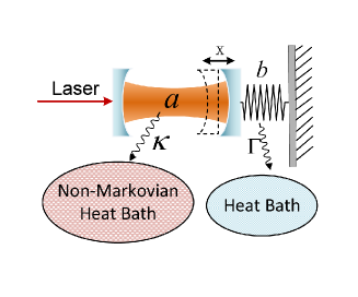
Figure 1: Schematic diagram of the optomechanical system, where the light field is considered to be in non-Markovian environment. The mechanical bath is set to be Markov to account for mechanical loss.

II Optomechanical model coupled to Non-Markovian environment

In this section, we introduce the optomechanical system and the non-Markovian environment that will be used to investigate chaos and entanglement. The optomechanical system is where a mechanical mode couples with an optical mode, as exhibited in Figure 1.

Assuming $\hbar=1$, the system is described by the Hamiltonian [1] given by

$$H_{s}=\big{[}-\Delta+g_{0}(b+b^{\dagger})\big{]}a^{\dagger}a+\Omega b^{\dagger}b+\alpha_{\textit{{L}}}(a^{\dagger}+a),$$ (1)

where $a$ and $b$ are the annihilation operators of the optical mode and mechanical mode which satisfy the commutation relations $[a,a^{\dagger}]=1$ and $[b,b^{\dagger}]=1$. $\Delta$ is the detuning parameter and $\Omega$ is the cantilever frequency. The detuning is defined as $\Delta\equiv\omega_{L}-\omega_{\mathrm{cav}}$, where $\omega_{L}$ is the pumping laser frequency and $\omega_{\mathrm{cav}}$ is the resonance frequency of the cavity mode $a$. $\alpha_{L}$ is the pumping laser amplitude and $g_{0}$ is the coupling constant between the two modes.

Since the optomechanical system is modelled as an open system, the cavity has radiative loss and cantilever has mechanical damping with respect to their local environments. The two baths are Bosonic, with the optical bath is set to be non-Markovian, which is the main focus of our study and can be adjusted experimentally [49]. While the mechanical bath is considered Markov to account for mechanical loss. The two baths are separated.

Using the first order approximation of the NMQSD equation [22], the master equation takes the form (details can be seen in Appendix A)

$$\dot{\rho}=-i[H_{s},\rho]+\Gamma D\big{[}b,\rho\big{]}+\bigg{\{}f_{0}(t)[a,\rho a^{\dagger}]+if_{1}(t)[a^{\dagger},[H_{s},a]\rho]+f_{2}(t)[a^{\dagger},[a^{\dagger},a]a\rho]+H.C.\bigg{\}},$$ (2)

where $H.C.$ stands for Hermitian conjugate. The Lindblad term $\Gamma D\big{[}b,\rho\big{]}=\Gamma\big{\{}b\rho b^{\dagger}-\frac{1}{2}(b^{\dagger}b\rho+\rho b^{\dagger}b)\big{\}}$ represents the Markov mechanical bath. $f_{0}$, $f_{1}$ and $f_{2}$ are time-dependent coefficients which are given by

$$\begin{split}&f_{0}(t)=\int_{0}^{t}\alpha(t,s)\;ds,\\ &f_{1}(t)=\int_{0}^{t}\alpha(t,s)(t-s)\;ds,\\ &f_{2}(t)=\int_{0}^{t}\int_{0}^{s}\alpha(t,s)\alpha(s,u)(t-s)\;du\;ds.\end{split}$$ (3)

$\alpha(t,s)$ is the Ornstein-Uhlenbeck (O-U) correlation function

$$\alpha(t,s)=\frac{\kappa\gamma}{2}e^{-\gamma|t-s|},$$ (4)

where $1/\gamma$ is the memory time, and $\kappa/\Omega=1$ is the optical damping rate.

We express the system parameters in units of $\Omega$ and introduce the dimensionless time parameter $\tau=\Omega t$. Additionally, we introduce two dimensionless variables [50, 51, 6]

$$\sigma=g_{0}/\kappa,\ P=\frac{8\alpha_{L}^{2}g_{0}^{2}}{\Omega^{4}}.$$ (5)

The pumping parameter $P$ gives the strength of the laser input of the cavity. The quantum-classical scaling parameter $\sigma$ is set to be $\sigma=x_{\mathrm{zpt}}/x_{\mathrm{res}}=g_{0}/\kappa=0.1$, where $x_{\mathrm{zpt}}=\sqrt{\hbar/(2m\Omega)}$ are the zero-point fluctuations of the cantilever (with mass $m$). Furthermore, $x_{\mathrm{res}}$ is the resonance width of the cavity, and $g_{0}$ is the optomechanical single-photon coupling strength [51, 6]. Since $x_{\mathrm{res}}$ is a classical quantity, $\sigma$ shows how close the quantum dynamics of the optomechanical system is to the classical limit, where $\sigma\to 0$ provides the classical limit.

We use the re-scaled creation and annihilation operators $\langle a_{1}\rangle=[\Omega/(2\alpha_{L})]\langle a\rangle$, $\langle b_{1}\rangle=(g_{0}/\Omega)\langle b\rangle$. Applying the trace expectation $\langle\dot{A}\rangle=tr(A\dot{\rho})$, the complete set of dynamical equations can be seen in Appendix B Eq. (27), here we give the first two equations

$$\begin{split}\frac{d}{d\tau}\langle a_{1}\rangle=&-i(1+f_{1})\bigg{\{}\langle a_{1}b_{1}\rangle+\langle a_{1}b_{1}^{\dagger}\rangle-\frac{\Delta}{\Omega}\langle a_{1}\rangle+\frac{1}{2}\bigg{\}}-\frac{f_{0}^{\ast}+f_{2}}{\Omega}\langle a_{1}\rangle,\\ \frac{d}{d\tau}\langle b_{1}\rangle=&-i\bigg{\{}\frac{P}{2}\langle a_{1}^{\dagger}a_{1}\rangle+\langle b_{1}\rangle\bigg{\}}-\frac{\Gamma}{2\Omega}\langle b_{1}\rangle.\end{split}$$ (6)

Eq. (27) forms a set of closed dynamical equations which will be used to investigate both chaos and entanglement of our system. Semi-classical (SC) approximation is made since the coupling $g_{0}$ is weak. Since the Hamiltonian is non-linear, an exact set of equations will have too many terms. Therefore, we use a SC approximation such that terms higher than second order are split.

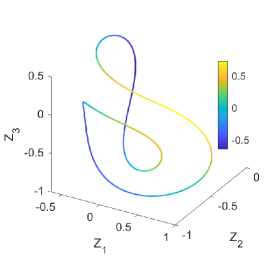
(a) $\gamma=10$

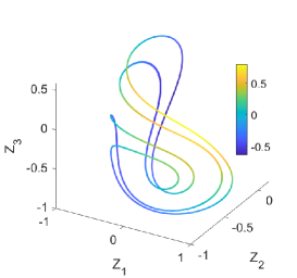
(b) $\gamma=2$

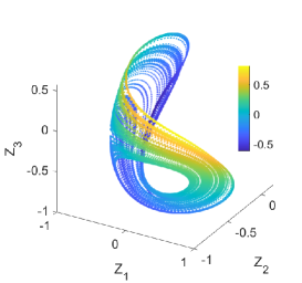
(c) $\gamma=0.8$

Figure 2: Phase diagrams with different correlation frequencies $\gamma$ at $\Delta=-0.70$, $P=1.25$. The coordinates $(Z_{1},Z_{2},Z_{3},Z_{4})$ are the real and imaginary parts of $\langle a_{1}\rangle$ and $\langle b_{1}\rangle$. The 4th coordinate $Z_{4}$ is represented by scaled colours. As memory time increases ($\gamma$ decreases), the dynamics goes from regular to chaotic. Fig. 2(c) exhibits the emerging of chaos as $\gamma$ is lowered to 0.8.

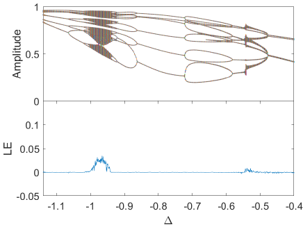
(a) $\gamma=10$

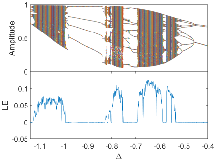
(b) $\gamma=2$

Figure 3: Bifurcation diagrams and corresponding Lyapunov exponents ($\bm{LE}$), with the laser pumping parameter $P=1.37$ and detuning varying from -1.2 to -0.4. In Fig. 3(a), the chaotic region is bounded within a small segment $\Delta\in[-1.03,-0.92]$. In Fig. 3(b), the chaotic region expanding to $\Delta\in[-1.13,-0.99]$ and a new chaotic region $\Delta\in[-0.83,-0.52]$ emerges, with some inter-adjacent regular regions inside.

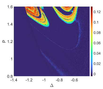
(a) $\gamma=10$

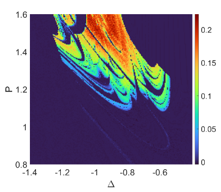
(b) $\gamma=1$

Figure 4: Pictures of chaotic regions of the optomechanical systems with different memory times plotted in the $P$-$\Delta$ plane. The colour scale shows the value of maximal Lyapunov exponent ($\bm{LE}$) of every data point. Comparing Fig. 4(a) and 4(b), the chaotic area expands as the memory time gets longer ($\gamma$ decreases).

III Chaos and Non-Markovian Environments

The mechanism of how a non-Markovian environment affects a chaotic system is the focus of this section. In general, chaotic systems tend to be very sensitive to parameter changes. The simulation methods used below allow one to manually adjust such a parameter, the non-Markovian memory time, which can have a delayed effect on the dissipative process of our open system. Such an effect may significantly influence chaos generation and therefore, we examine various memory times and their effects of chaos generation.

Our simulation is mainly based on observing the optomechanical system while changing the memory time of the optical bath represented by the parameter $\gamma$ (the inverse of memory time). Furthermore, we vary the system parameters $\Delta$ and $P$ to get a comprehensive picture of the chaos distribution of our system. The initial states are set to be the vacuum states. We use the maximal Lyapunov exponent ($\bm{LE}$) as the indicator of chaos, which is calculated using the Wolf’s method of phase reconstruction [52]. If the $\bm{LE}$ is positive, the system is considered to be chaotic.

By taking the real and imaginary parts of the time series of $\langle a_{1}\rangle$ and $\langle b_{1}\rangle$ from Eq. (27), we can generate the four-dimensional phase diagrams based on different memory times (the inverse of $\gamma$). Figure (2) below illustrates the system dynamics under different memory times for a fixed point ($P=1.25$ and $\Delta=-0.70$). The increase of $\gamma$ results in the system changing from regular to chaotic, which serves as a key example of memory induced chaos.

Next, we plot the bifurcation diagrams which mark the stable points of the cantilever oscillation. We fix $P=1.37$. At $\gamma=10$, the period-doubling bifurcation takes place, as is exhibited in Fig. (3(a)), where the chaotic region is bounded within a small segment $\Delta\in[-1.03,-0.92]$. For the $\gamma=2$ case, Fig. (3(b)) shows the chaotic region expanding to $\Delta\in[-1.13,-0.99]$ while a new chaotic region at $\Delta\in[-0.83,-0.52]$ emerges, with some inter-adjacent regular regions inside. The comparison between Fig. (3(a)) and (3(b)) clearly indicates that the longer memory time can, not only expand chaotic regions, but also induce chaos from the previously non-chaotic areas. Note that $\gamma=2$ is not far away from the Markov limit, but it still causes significant change to chaotic dynamics, further indicating that the chaos is very sensitive to parameter changes, including the memory time.

To summarize the appearances of chaos, the $\bm{LE}$ of every data point is plotted to form global chaos landscapes, as is shown in Fig. (4(a)) for $\gamma=10$ and (4(b)) for $\gamma=1$. The parameter ranges are set to be $P\in[0.8,1.6]$ and $\Delta\in[-1.4,-0.4]$. As the pumping increases, we see more chaotic motion [6, 51, 50]. In both cases, the chaotic regions have some fine structures of inter-adjacent regular regions. For our model, we have shown that the non-Markovian condition expands the chaotic regions while lowering the pumping bar for chaos generation. For the the case of $\gamma=10$ (Fig. 4(a)), the chaos emerging level is $P=1.37$, while for $\gamma=1$ (Fig. 4(b)), the level is lowered to $P=1.08$.

Comparing Fig. (4(a)) and (4(b)), we have seen that the increase of memory time can expand chaotic areas in the parameter plane and decrease the pumping threshold for chaos generation. While the amplitude damping is the major dissipating channel, the environmental memory can slow down the dissipation of energy. The dissipative dynamics will undergo temporal revivals due to the memory effect. This results in the emerging of chaos that requires less pumping energy, thus lowering the pumping threshold while expanding chaotic regions across the map. A similar phenomena has been discussed in [48] where the memory enhanced entanglement generation was also due to the back-flow in the dissipation channel in the form of information. Since energy carries information, our model can be understood in a similar fashion.

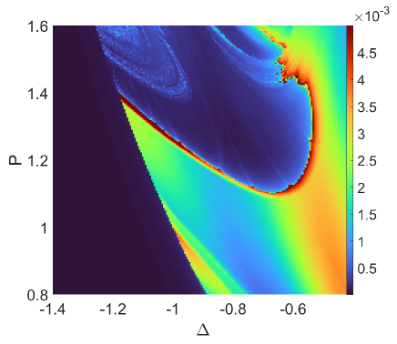
(a) $\gamma=10$

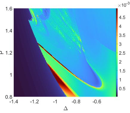
(b) $\gamma=1$

Figure 5: The entanglement strength $\bm{En}$ on the $P$-$\Delta$ plane. The colour scale measures the value of $\bm{En}$. The entanglement shows similar fine structures as the chaos.

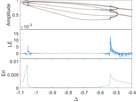
(a) $P=1.3$

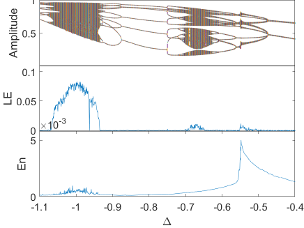
(b) $P=1.4$

Figure 6: Bifurcation diagram, maximal Lyapunov exponent ($\bm{LE}$), comparing with average negativity of the partial transposition ($\bm{En}$), when $\gamma=10$.

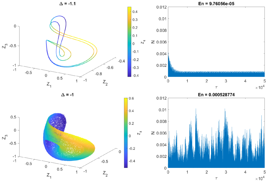
Figure 7: Phase diagram and the corresponding long term dynamical evolution of the NPT $\mathcal{N}$, with $P=1.4$. The first roll shows $\Delta=-1.1$ (non-chaotic) and the second roll $\Delta=-1.0$ (chaotic). The dynamical evolution of $\mathcal{N}$ appears solid simply because it is oscillating very quickly.

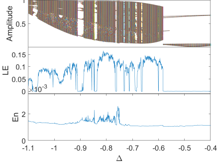
(a) $P=1.3$

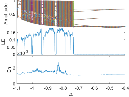
(b) $P=1.4$

Figure 8: Bifurcation diagram, maximal Lyapunov exponent ($\bm{LE}$), comparing with average negativity of the partial transposition ($\bm{En}$), when $\gamma=1$.

IV Entanglement and Chaos

We now turn to the quantum aspects of our optomechanical system to investigate entanglement under the presence of chaos and memory time. The optomechanical system we are studying is a weakly coupled bipartite system. There have been several studies focusing on chaos and its effects on entanglement [53, 54, 55, 41, 56, 57]. One previous study looks at the effects of environment memory on entanglement [48].

Since the non-linear Hamiltonian of our system (1) causes our physical states to be non-Gaussian, the conventional ways of calculating inseparability [58, 59, 60] would cause imaginary terms that cannot be ignored. Therefore, a non-conventional method is needed to calculate the entanglement of the two modes of our system. Here, we will use a hierarchy of necessary and sufficient conditions for the negativity of the partial transposition (NPT) in terms of observable moments [42]. Though this leads only to sufficient conditions for entanglement, it can be applied to a variety of quantum states (including non-Gaussian states).

IV.1 Entanglement Measurement

A brief introduction of Shchukin and Vogel’s (SV) criterion is provided here [42]. It is known that a bipartite quantum state is entangled if NPT is achieved [43, 61]. We start with a separable bipartite state $\hat{\rho}$. The condition for its separability is that its partial transposed density operator $\hat{\rho}^{\text{PT}}$ can be written in the following form (assuming that we are transposing the second Hilbert space state, which won’t affect our result)

$$\hat{\rho}^{\text{PT}}=\sum^{\infty}_{n=0}p_{n}\hat{\rho}^{(n)}_{1}\otimes\hat{\rho}^{(n)\text{T}}_{2}.$$ (7)

Based on this property of separable states, we can employ NPT as a sufficient condition for inseparability, which is referred to as the Peres-Horodecki condition [61, 62, 63]. The separability is determined through a matrix of moments of the partial transposition, which is given by

$$M_{pqrs,nmkl}=\langle a^{\dagger q}a^{p}a^{\dagger n}a^{m}b^{\dagger s}b^{r}b^{\dagger k}b^{l}\rangle^{\text{PT}}.$$ (8)

Shchukin and Vogel [42] introduced a way of ordering the moments $M_{pqrs,nmkl}$ as follows

$$\begin{split}&1,\ \langle a\rangle,\ \langle a^{\dagger}\rangle,\ \langle b\rangle,\ \langle b^{\dagger}\rangle,\ \langle a^{2}\rangle,\ \langle a^{\dagger}a\rangle,\ \langle a^{\dagger 2}\rangle,\ \langle ab\rangle,\\ &\langle a^{\dagger}b\rangle,\ \langle b^{2}\rangle,\ \langle ab^{\dagger}\rangle,\ \langle a^{\dagger}b^{\dagger}\rangle,\ \langle b^{\dagger}b\rangle,\ \langle b^{\dagger 2}\rangle,\ ...\end{split}$$ (9)

The moments $M_{pqrs,nmkl}$ in Eq. (8) can be expressed in terms of the moments of the original state

$$\langle a^{\dagger q}a^{p}a^{\dagger n}a^{m}b^{\dagger s}b^{r}b^{\dagger k}b^{l}\rangle^{\text{PT}}=\langle a^{\dagger q}a^{p}a^{\dagger n}a^{m}b^{\dagger l}b^{k}b^{\dagger r}b^{s}\rangle.$$ (10)

For our quantum state, it is convenient to use a higher-order test involving a small number of minors, which was introduced in [43]. The matrix determinant is given as follows (using the re-scaled $a_{1}$ and $b_{1}$)

$$D_{HO}=\begin{vmatrix}1&\langle a_{1}b_{1}^{\dagger}\rangle\\ \langle a_{1}^{\dagger}b_{1}\rangle&\langle a_{1}^{\dagger}a_{1}b_{1}^{\dagger}b_{1}\rangle\end{vmatrix}.$$ (11)

If there exist a negative determinant

$$D_{HO}<0,$$ (12)

then the NPT has been demonstrated, which provides a sufficient condition for entanglement. Conveniently, the set of mean values are already provided by the semi-classical equations of motion (27), and the SC approximation is used such that $\langle a_{1}^{\dagger}a_{1}b_{1}^{\dagger}b_{1}\rangle=\langle a_{1}^{\dagger}a_{1}\rangle\langle b_{1}^{\dagger}b_{1}\rangle$.

We define $\mathcal{N}$ to denote the negativity of the partial transposition (NPT)

$$\mathcal{N}=\mathrm{max}[0,-D_{HO}].$$ (13)

A positive value for $\mathcal{N}$ indicates that the states are entangled. We then define $\bm{En}$ as the long-time average of $\mathcal{N}(t)$ [56]. It provides an overview of the entanglement intensity as is given by

$$\bm{En}=\frac{1}{T}\int_{0}^{T}\mathcal{N}(t)dt,$$ (14)

where $T\to\infty$. Since $\bm{En}$ is only determined by parameters $P$, $\Delta$ and $\gamma$, we can calculate the averge NPT ($\bm{En}$) of every data point analogous to the $\bm{LE}$ for chaos.

IV.2 Simulation Results

The following simulations show the quantum entanglement under the influence of chaotic motion and non-Markovian environment. We consider two memory parameters, namely the close to Markov case and the non-Markovian case.

First, we focus on the close to Markov case, with $\gamma=10$. Overall, the graph (Fig. 5(a)) of average NPT ($\bm{En}$) on the parameter plane reflects almost the same fine structure as the chaos graph (Fig. 4(a)). It is worth noting that the very small $\bm{LE}$ spikes in Fig. (4(a)) coincide with sharp $\bm{En}$ spikes. To provide a closer look, we show the bifurcation, $\bm{LE}$, and $\bm{En}$ diagrams, fixing $\gamma=10$. With $P=1.3$, Fig. (6(a)) shows two very small $\bm{LE}$ spikes coincide with two huge $\bm{En}$ spikes. Fig. (6(b)) demonstrates that the chaotic area $\Delta\in[-1.066,-0.94]$ corresponding to an area of entanglement increase. As shown in Fig. (7), the chaos can enhance the bipartite entanglement for the non-linear optomechanical system, our results are in tune with the observations for a quantum kicked top system [56]. In summary, the bipartite entanglement generation can be increased by classical chaotic dynamics. However, it should be noted that the $\bm{En}$ level (as shown in Fig. 4(a)) can be lower than some non-chaotic areas on the parameter plane meaning that the enhancement effect of entanglement by chaos is localized (on the parameter plane).

Furthermore, in the non-Markovian $\gamma=1$ case (Fig. 5(b)), we can still see some fine structures related to the chaos graph (Fig. 4(b)), where the $\bm{En}$ level around chaotic areas is larger than the $\gamma=10$ case (Fig. 4(a)). In Fig. (8(b)), we can observe the slight enhancement of entanglement by chaos. Yet, that effect dies down at $\Delta>-0.78$ while in Fig. (8(a)), it terminates at $\Delta>-0.74$. Overall, the $\bm{En}$ level is higher than the $\gamma=10$ case and the distinction of $\bm{En}$ between chaotic and non-chaotic areas is much less, which is similar to the results demonstrated in a linear optomechanical system [48], whose explanation is that the memory effect creates information back flow such that the dissipative dynamics will experience temporal revivals. The dissipation and the back flow from the environment may reach a new balance point so that the steady state entanglement ($t\to\infty$) may be dependent on its memory. The result of this mechanics is the enhancement of entanglement by the environmental memory time, in our non-linear optomechanical system. Though this effect is still localized, as one cannot tell whether all areas on Fig. (5(b)) have higher $\bm{En}$ than Fig. (5(a)). In summary, both the environmental memory and the chaotic dynamics can significantly affect entanglement generation.

V Conclusion

We have analyzed classical chaos in a non-Markovian optomechanical system and measured the corresponding quantum entanglement. We have shown that environmental memory can increase chaos generation in the optomechanical system. For the non-linear optomechanical system, it is shown that the memory effect causes the energy back flow resulting in the chaos region expanding while lowering the pumping bar for chaos generation. As for the entanglement, we observed two effects. The first one is that bipartite entanglement is sensitive to chaos and can be enhanced by it. The second effect is that the environmental memory time can increase bipartite entanglement generation. In conclusion, in the non-linear optomechanical system, non-Markovian memory time can be an enhancing factor for classical chaos generation, while chaos and environmental memory both can increase entanglement generation.

Appendix A The non-Markovian quantum state diffusion (NMQSD) equation

The following section provides a detailed derivation of the non-Markovian master equation.

Both environments are set to be at zero temperature, and separate from each other. Since the Markov environment is well-understood and its formation can be added to the master equation easily, we can focus on the optical bath and use the non-Markovian quantum state diffusion (QSD) equation to derive the master equation.

The non-Markovian bath for the optical mode can be described by a set of harmonic oscillators [48]

$$H_{B}=\sum_{j}\omega_{j}c^{\dagger}_{j}c_{j},$$ (15)

where $c_{j}$ and $c_{j}^{\dagger}$ are annihilation and creation operators satisfying the commutation relation $[c_{i},c_{j}^{\dagger}]=\delta_{ij}$. In general, the interaction Hamiltonian between the system and its Bosonic bath is described by

$$H_{I}=\sum_{j}g_{j}(Lc^{\dagger}_{j}+L^{\dagger}c_{j}),$$ (16)

where $L=a$ is the Lindblad operator representing the optical damping and $g_{j}$ are the system-bath coupling intensities. The interaction Hamiltonian is in the form of a rotating wave approximation which assumes the condition of weak coupling strength ($g_{j}\ll\Omega$).

Assuming the optomechanical system and the environment are not correlated initially, the state of the optomechanical system connecting to a non-Markovian bath can be represented by the non-Markovian quantum state diffusion (NMQSD) equation [23, 21] governing the time evolution of the a stochastic pure state $|\psi_{t}(z^{\ast})\rangle$, which is given by

$$\partial_{t}|\psi_{t}(z^{\ast})\rangle=\bigg{[}-iH_{s}+az^{\ast}_{t}-a^{\dagger}\overline{O}(t,z^{\ast})\bigg{]}|\psi_{t}(z^{\ast})\rangle,$$ (17)

where $O(t,s,z^{\ast})\psi_{t}\equiv\frac{\delta\psi_{t}}{\delta z_{s}}$ and $\overline{O}(t,z^{\ast})\equiv\int^{t}_{0}ds\alpha(t,s)O(t,s,z^{\ast})$ with the initial condition $O(t,s=t,z^{\ast})=a$. $\alpha(t,s)=\frac{\kappa\gamma}{2}e^{-\gamma|t-s|}$ is the Ornstein-Uhlenbeck (O-U) correlation function. $z_{t}^{\ast}=-i\sum_{j}g_{j}z^{\ast}_{j}e^{i\omega_{j}t}$ is a colored complex Gaussian process satisfying

$$M[z_{t}^{\ast}z_{s}]=\alpha(t,s).\ M[z_{t}z_{s}]=0,$$ (18)

where $M[\cdot]\equiv\int\frac{dz^{2}}{\pi}e^{-|z|^{2}}[\cdot]$ denotes the ensemble average over the noise $z_{t}$.

To solve (17), one needs to find the operator $O(t,s,z^{\ast})$. Under the condition that the memory time is not too long, we consider the expansion of $O(t,s,z^{\ast})$ in powers of $(t-s)$ [22]

$$O(t,s,z^{\ast})=O(s,s,z^{\ast})+\frac{\partial O(t,s,z^{\ast})}{\partial t}\bigg{|}_{t=s}(t-s)+\cdots,$$ (19)

which is a systematic expansion of the non-Markovian QSD. The zeroth-order term corresponds to the standard Markov QSD when $1/\gamma\to 0$. We choose the first-order approximation of the operator $O(t,s,z^{\ast})$ since the first-order term is the most important correction to Markovian dynamics given that the memory time is assumed to be short.

At the time point $t=s$, the expression of the operator $O(t,s,z^{\ast})$ is given by [22]

$$O(s,s,z^{\ast}) =a,$$ (20)

$$\frac{\partial O(t,s,z^{\ast})}{\partial t}\bigg{|}_{t=s} =-i[H_{s},a]-\int^{s}_{0}\alpha(s,u)du[a^{\dagger},a]a,$$ (21)

where $H_{s}$ is the system Hamiltonian and $a$ is the Lindblad operator. At this time point, the operator $\overline{O}$ becomes

$$\overline{O}=f_{0}(t)a-f_{1}(t)i[H_{s},a]-f_{2}(t)[a^{\dagger},a]a,$$ (22)

where

$$\begin{split}&f_{0}(t)=\int_{0}^{t}\alpha(t,s)\;ds,\\ &f_{1}(t)=\int_{0}^{t}\alpha(t,s)(t-s)\;ds,\\ &f_{2}(t)=\int_{0}^{t}\int_{0}^{s}\alpha(t,s)\alpha(s,u)(t-s)\;du\;ds.\end{split}$$ (23)

One can turn (17) into a master equation by taking the ensemble mean over the noise $z_{t}$ and introducing the reduced density matrix $\rho_{t}=M[|\psi_{t}(z^{\ast})\rangle\langle\psi_{t}(z^{\ast})|]$. When the environment is not far away from Markov, the dependence of the operator $\overline{O}(t,z^{\ast})$ on the noise $z_{t}$ is negligible. Under this approximation, the master equation [22] takes the form

$$\frac{d}{dt}\rho_{t}=-i[H_{s},\rho_{t}]+[a,\rho_{t}\overline{O}(t)^{\dagger}]-[a^{\dagger},\overline{O}(t)\rho_{t}].$$ (24)

For further details about the derivation of the master equation, see [24, 28].

Since the mechanical bath is separate and Markov, it can be added to the master equation by simply including the appropriate Lindblad term which is given by

$$\Gamma D\big{[}b,\rho\big{]}=\Gamma\big{\{}b\rho b^{\dagger}-\frac{1}{2}(b^{\dagger}b\rho+\rho b^{\dagger}b)\big{\}},$$ (25)

where $\Gamma/\Omega=10^{-3}$ is the mechanical damping.

Using the first order approximation of $\overline{O}(t)$ (22), the master equation takes the final form

$$\dot{\rho}=-i[H_{s},\rho]+\Gamma D\big{[}b,\rho\big{]}+\bigg{\{}f_{0}(t)[a,\rho a^{\dagger}]+if_{1}(t)[a^{\dagger},[H_{s},a]\rho]+f_{2}(t)[a^{\dagger},[a^{\dagger},a]a\rho]+H.C.\bigg{\}},$$ (26)

where $H.C.$ stands for Hermitian conjugate.

Appendix B The complete set of dynamical equations

$$\begin{split}\frac{d}{d\tau}\langle a_{1}\rangle=&-i(1+f_{1})\bigg{\{}\langle a_{1}b_{1}\rangle+\langle a_{1}b_{1}^{\dagger}\rangle-\frac{\Delta}{\Omega}\langle a_{1}\rangle+\frac{1}{2}\bigg{\}}-\frac{f_{0}^{\ast}+f_{2}}{\Omega}\langle a_{1}\rangle,\\ \frac{d}{d\tau}\langle b_{1}\rangle=&-i\bigg{\{}\frac{P}{2}\langle a_{1}^{\dagger}a_{1}\rangle+\langle b_{1}\rangle\bigg{\}}-\frac{\Gamma}{2\Omega}\langle b_{1}\rangle,\\ \frac{d}{d\tau}\langle a_{1}^{\dagger}a_{1}\rangle=&-\frac{i}{2}(\langle a_{1}^{\dagger}\rangle-\langle a_{1}\rangle)-\frac{1}{\Omega}(f_{0}+f_{0}^{\ast}+f_{2}+f_{2}^{\ast})\langle a_{1}^{\dagger}a_{1}\rangle\\ &+i(f_{1}^{\ast}-f_{1})(-\frac{\Delta}{\Omega}+\langle b_{1}^{\dagger}\rangle+\langle b_{1}\rangle)\langle a_{1}^{\dagger}a_{1}\rangle+\frac{i}{2}(f_{1}^{\ast}\langle a_{1}\rangle-f_{1}\langle a_{1}^{\dagger}\rangle),\\ \frac{d}{d\tau}\langle b_{1}^{\dagger}b_{1}\rangle=&-i\frac{P}{2}\langle a_{1}^{\dagger}a_{1}\rangle(\langle b^{\dagger}_{1}\rangle-\langle b_{1}\rangle)-\frac{\Gamma}{\Omega}\langle b_{1}^{\dagger}b_{1}\rangle,\\ \frac{d}{d\tau}\langle a_{1}^{2}\rangle=&-2i(1+f_{1})\bigg{\{}(-\frac{\Delta}{\Omega}+\langle b_{1}^{\dagger}\rangle+\langle b_{1}\rangle)\langle a_{1}^{2}\rangle+\frac{\langle a_{1}\rangle}{2}\bigg{\}}-\frac{2}{\Omega}(f_{0}^{\ast}+f_{2})\langle a_{1}^{2}\rangle,\\ \frac{d}{d\tau}\langle b_{1}^{2}\rangle=&-2i\bigg{\{}\frac{P}{2}\langle a_{1}^{\dagger}a_{1}\rangle\langle b_{1}\rangle+\langle b_{1}^{2}\rangle\bigg{\}}-\frac{\Gamma}{\Omega}\langle b_{1}^{2}\rangle,\\ \frac{d}{d\tau}\langle a_{1}b_{1}\rangle=&-i(1+f_{1})\bigg{\{}(\langle b_{1}^{2}\rangle+\langle b_{1}^{\dagger}b_{1}\rangle)a_{1}-\frac{\Delta}{\Omega}\langle a_{1}b_{1}\rangle+\frac{1}{2}\langle b_{1}\rangle\bigg{\}}\\ &-i\bigg{\{}\langle a_{1}b_{1}\rangle+\frac{P}{2}\langle a_{1}^{\dagger}a_{1}\rangle\langle a_{1}\rangle+(\frac{g_{0}}{\Omega})^{2}\langle a_{1}\rangle\bigg{\}}-\frac{1}{\Omega}(f_{0}^{\ast}+f_{2})\langle a_{1}b_{1}\rangle,\\ \frac{d}{d\tau}\langle a_{1}b_{1}^{\dagger}\rangle=&-i(1+f_{1})\bigg{\{}(\langle b_{1}^{\dagger 2}\rangle+\langle b_{1}^{\dagger}b_{1}\rangle)a_{1}+(\frac{g_{0}}{\Omega})^{2}\langle a_{1}\rangle-\frac{\Delta}{\Omega}\langle a_{1}b_{1}^{\dagger}\rangle+\frac{1}{2}\langle b_{1}^{\dagger}\rangle\bigg{\}}\\ &+i\bigg{\{}\langle a_{1}b_{1}^{\dagger}\rangle+\frac{P}{2}\langle a_{1}^{\dagger}a_{1}\rangle\langle a_{1}\rangle+(\frac{g_{0}}{\Omega})^{2}\langle a_{1}\rangle\bigg{\}}-\frac{1}{\Omega}(f_{0}^{\ast}+f_{2})\langle a_{1}b_{1}^{\dagger}\rangle,\end{split}$$ (27)

where we have used the relations (in terms of $a$ and $b$)

$$\begin{split}&\langle a^{\dagger}\rangle=\langle a\rangle^{\ast},\ \langle b^{\dagger}\rangle=\langle b\rangle^{\ast},\ \langle aa^{\dagger}\rangle=\langle a^{\dagger}a\rangle+1,\\ &\langle bb^{\dagger}\rangle=\langle b^{\dagger}b\rangle+1,\ \langle a^{\dagger 2}\rangle=\langle a^{2}\rangle^{\ast},\ \langle b^{\dagger 2}\rangle=\langle b^{2}\rangle^{\ast},\\ &\langle a^{\dagger}b^{\dagger}\rangle=\langle ab\rangle^{\ast},\ \langle a^{\dagger}b\rangle=\langle ab^{\dagger}\rangle^{\ast}.\end{split}$$ (28)

References

- Aspelmeyer et al. [2014] M. Aspelmeyer, T. J. Kippenberg, and F. Marquardt, Rev. Mod. Phys. 86, 1391 (2014).
- Jiang et al. [2017] X. F. Jiang, L. B. Shao, S. X. Zhang, X. Yi, J. Wiersig, L. Wang, Q. H. Gong, M. Loncar, L. Yang, and Y. F. Xiao, Science 358, 344 (2017).
- Sciamanna [2016] M. Sciamanna, Nat. Photon. 10, 366 (2016).
- Monifi et al. [2016] F. Monifi, J. Zhang, S. K. Özdemir, B. Peng, Y. X. Liu, F. Bo, F. Nori, and L. Yang, Nat. Photon. 10, 399 (2016).
- Navarro-Urrios et al. [2017] D. Navarro-Urrios, N. E. Capuj, M. F. Colombano, P. D. Garcia, M. Sledzinska, F. Alzina, A. Griol, A. Martinez, and C. M. Sotomayor-Torres, Nat. Commun. 8, 14965 (2017).
- Bakemeier et al. [2015] L. Bakemeier, A. Alvermann, and H. Fehske, Phys. Rev. Lett. 114, 013601 (2015).
- Carmon et al. [2007] T. Carmon, M. C. Cross, and K. J. Vahala, Phys. Rev. Lett. 98, 167203 (2007).
- Larson and Horsdal [2011] J. Larson and M. Horsdal, Phys. Rev. A 84, 021804(R) (2011).
- Lee et al. [2009] S. B. Lee, J. Yang, S. Moon, S. Y. Lee, J. B. Shim, S. W. Kim, J. H. Lee, and K. An, Phys. Rev. Lett. 103, 134101 (2009).
- Lü et al. [2015] X. Y. Lü, H. Jing, J. Y. Ma, and Y. Wu, Phys. Rev. Lett. 114, 253601 (2015).
- Piazza and Ritsch [2015] F. Piazza and H. Ritsch, Phys. Rev. Lett. 115, 163601 (2015).
- Sun and Sukhorukov [2014] Y. Sun and A. A. Sukhorukov, Opt. Lett. 39, 3543 (2014).
- Walter and Marquardt [2016] S. Walter and F. Marquardt, New J. Phys. 18, 113029 (2016).
- Wang et al. [2014] G. L. Wang, L. Huang, Y. C. Lai, and C. Grebogi, Phys. Rev. Lett. 112, 110406 (2014).
- Yang et al. [2015] N. Yang, J. Zhang, H. Wang, Y. X. Liu, R. B. Wu, L. Q. Liu, C. W. Li, and F. Nori, Phys. Rev. A 92, 033812 (2015).
- Dalibard et al. [1992] J. Dalibard, Y. Castin, and K. Mølmer, Phys. Rev. Lett. 68, 580 (1992).
- Gisin and Percival [1992] N. Gisin and I. C. Percival, J. Phys. A: Math. Gen. 25, 5677 (1992).
- Carmichael [1993] H. Carmichael, An Open Systems Approach to Quantum Optics Springer-Verlag (Springer Berlin, Heidelberg, Berlin, 1993).
- Wiseman and Milburn [1993] H. M. Wiseman and G. J. Milburn, Phys. Rev. A 47, 1652 (1993).
- Plenio and Knight [1998] M. B. Plenio and P. L. Knight, Rev. Mod. Phys. 70, 101 (1998).
- Strunz et al. [1999] W. T. Strunz, L. Diósi, and N. Gisin, Phys. Rev. Lett. 82, 1801 (1999).
- Yu et al. [1999] T. Yu, L. Diósi, N. Gisin, and W. T. Strunz, Phys. Rev. A 60, 91 (1999).
- Diósi et al. [1998] L. Diósi, N. Gisin, and W. T. Strunz, Phys. Rev. A 58, 1699 (1998).
- Strunz and Yu [2004] W. T. Strunz and T. Yu, Phys. Rev. A 69, 052115 (2004).
- Yu [2004] T. Yu, Phys. Rev. A 69, 062107 (2004).
- Jing and Yu [2010] J. Jing and T. Yu, Phys. Rev. Lett. 105, 240403 (2010).
- Yang et al. [2012] H. Yang, H. Miao, and Y. Chen, Phys. Rev. A 85, 040101 (2012).
- Chen et al. [2014] Y. Chen, J. Q. You, and T. Yu, Phys. Rev. A 90, 052104 (2014).
- Xu et al. [2014] J. Xu, X. Zhao, J. Jing, L. A. Wu, and T. Yu, J. Phys. A: Math. Theor. 47, 435301 (2014).
- Moon [1992] F. C. Moon, Chaotic and Fractal Dynamics: An Introduction for Applied Scientists and Engineers (Wiley, Hoboken, 1992).
- Strogatz [2001] S. H. Strogatz, Nonlinear Dynamics and Chaos: With Applications to Physics, Biology, Chemistry, and Engineering (Westview Press, Boulder, 2001).
- Poulin [2002] D. Poulin, Physics Department and IQC, University of Waterloo (2002).
- Field et al. [1995] S. Field, N. Venturi, and F. Nori, Phys. Rev. Lett. 74, 74 (1995).
- Field et al. [1997] S. B. Field, M. Klaus, M. G. Moore, and F. Nori, Nature 388, 252 (1997).
- Nakamura [1993] K. Nakamura, Quantum Chaos: A New Paradigm of Nonlinear Dynamics (Cambridge University Press, Cambridge, 1993).
- Heller [1984] E. J. Heller, Phys. Rev. Lett. 53, 1515 (1984).
- Heller [2018] E. J. Heller, The semiclassical way to dynamics and spectroscopy (Princeton University Press, 2018).
- Gutzwiller [1990] M. C. Gutzwiller, Chaos in classical and quantum mechanics (Springer Verlag, New York, 1990).
- Ullmo [2008] D. Ullmo, Rep. Prog. Phys. 71, 026001 (2008).
- Wright and Weaver [2010] M. Wright and R. Weaver, New directions in linear acoustics and vibration: quantum chaos, random matrix theory and complexity (Cambridge University Press, 2010).
- Fujisaki et al. [2003] H. Fujisaki, T. Miyadera, and A. Tanaka, Phys. Rev. E 67, 066201 (2003).
- Shchukin and Vogel [2005] E. Shchukin and W. Vogel, Phys. Rev. Lett. 95, 230502 (2005).
- Gomes et al. [2009] R. M. Gomes, A. Salles, F. Toscano, P. H. Souto Ribeiro, and S. P. Walborn, Proc. Natl. Acad. Sci. 106, 21517 (2009).
- Chou et al. [2008] C. H. Chou, T. Yu, and B. L. Hu, Phys. Rev. E 77, 011112 (2008).
- Paz and Roncaglia [2008] J. P. Paz and A. J. Roncaglia, Phys. Rev. Lett. 100, 220401 (2008).
- Wang and Clerk [2013] Y. D. Wang and A. A. Clerk, Phys. Rev. Lett. 110, 253601 (2013).
- Cheng et al. [2016] J. Cheng, W. Z. Zhang, L. Zhou, and W. Zhang, Sci. Rep. 6, 1 (2016).
- Mu et al. [2016] Q. Mu, X. Zhao, and T. Yu, Phys. Rev. A 94, 012334 (2016).
- Liu et al. [2011] B. H. Liu, L. Li, Y. F. Huang, C. F. Li, G. C. Guo, E. M. Laine, H. P. Breuer, and J. Piilo, Nat. Phys. 7, 931 (2011).
- Marquardt et al. [2006] F. Marquardt, J. G. E. Harris, and S. M. Girvin, Phys. Rev. Lett. 96, 103901 (2006).
- Ludwig et al. [2008] M. Ludwig, B. Kubala, and F. Marquardt, New J. Phys. 10, 095013 (2008).
- Wolf et al. [1985] A. Wolf, J. B. Swift, H. L. Swinney, and J. A. Vastano, Physica D 16, 285 (1985).
- Furuya et al. [1998] K. Furuya, M. C. Nemes, and G. Q. Pellegrino, Phys. Rev. Lett. 80, 5524 (1998).
- Lakshminarayan [2001] A. Lakshminarayan, Phys. Rev. E 64, 036207 (2001).
- Bandyopadhyay and Lakshminarayan [2002] J. N. Bandyopadhyay and A. Lakshminarayan, Phys. Rev. Lett. 89, 060402 (2002).
- Wang et al. [2004] X. Wang, S. Ghose, B. C. Sanders, and B. Hu, Phys. Rev. E 70, 016217 (2004).
- Ghose and Sanders [2004] S. Ghose and B. C. Sanders, Phys. Rev. A 70, 062315 (2004).
- Simon [2000] R. Simon, Phys. Rev. Lett. 84, 2726 (2000).
- Duan et al. [2000] L. M. Duan, G. Giedke, J. I. Cirac, and P. Zoller, Phys. Rev. Lett. 84, 2722 (2000).
- Adesso et al. [2004] G. Adesso, A. Serafini, and F. Illuminati, Phys. Rev. A 70, 022318 (2004).
- Peres [1996] A. Peres, Phys. Rev. Lett. 77, 1413 (1996).
- Horodecki et al. [1996] R. Horodecki, M. Horodecki, and P. Horodecki, Phys. Rev. A 222, 21 (1996).
- Horodecki et al. [2001] M. Horodecki, P. Horodecki, and R. Horodecki, Phys. Rev. A 283, 1 (2001).