Optimization-based Sensitivity Analysis for Unmeasured Confounding using Partial Correlations

Abstract

Causal inference necessarily relies upon untestable assumptions; hence, it is crucial to assess the robustness of obtained results to violations of identification assumptions. However, such sensitivity analysis is only occasionally undertaken in practice, as many existing methods only apply to relatively simple models and their results are often difficult to interpret. We take a more flexible approach to sensitivity analysis and view it as a constrained stochastic optimization problem. This work focuses on sensitivity analysis for a linear causal effect when an unmeasured confounder and a potential instrument are present. We show how the bias of the OLS and TSLS estimands can be expressed in terms of partial correlations. Leveraging the algebraic rules that relate different partial correlations, practitioners can specify intuitive sensitivity models which bound the bias. We further show that the heuristic “plug-in” sensitivity interval may not have any confidence guarantees; instead, we propose a bootstrap approach to construct sensitivity intervals which perform well in numerical simulations. We illustrate the proposed methods with a real study on the causal effect of education on earnings and provide user-friendly visualization tools.

1 Introduction

In many scientific disciplines, provisional causal knowledge is predominantly generated from observational data as randomized controlled experiments are often infeasible or too costly. Because the treatment is not randomly assigned in an observational study, any causal conclusions must rely on untestable assumptions, such as absence of unmeasured confounders or validity of instrumental variables. Hence, the causal inference is inherently sensitive to violations of any identification and modelling assumptions, so reseachers are advised to investigate the robustness of their results.

The importance of sensitivity analysis has been emphasized in guidelines for designing and reporting observational studies (Vandenbroucke et al., 2007; PCORI Methodology Committee, 2021). For instance, the STROBE guidelines caution that “taking [observed] confounders into account is crucial in observational studies, but readers should not assume that analyses adjusted for [observed] confounders establish the ‘causal part’ of an association” (p. 1638). They recommend to conduct sensitivity analyses as they are “helpful to investigate the influence of choices made in the statistical analysis, or to investigate the robustness of the findings to missing data or possible biases” (p. 1647).

However, sensitivity analysis is still rarely conducted in actual studies, making it difficult for other researchers to assess the robustness of their empirical findings. In medicine, Thabane et al. (2013) did a spot check on the January 2012 editions of major medical journals and found that only 26.7% (36 out of 135) of the articles that included some statistical analysis also performed sensitivity analysis. In nutrition research, de Souza et al. (2016) found that, in a representative sample of 100 articles from 2013 to 2015, merely 18% of them conducted some sensitivity analysis. In political science, Cinelli and Hazlett (2020) found that only 4 out of 64 observational studies published in three leading journals in 2017 conducted a formal sensitivity analysis beyond mere model specification checks.

There are several reasons for the hesitant uptake of sensitivity analysis in practice. First, it is not straightforward to define a reasonable model for sensitivity analysis, even for the familiar setting of one treatment variable, one outcome variable, and multiple baseline covariates that has been studied since the seminal work of Cornfield et al. (1959). For example, Lin et al. (1998) assume an unmeasured confounder $U$ independent of the measured covariates $X$ conditional on the treatment. However, Hernan and Robins (1999) point out that this assumption may be implausible as conditioning on the treatment opens a collider path between $U$ and $X$. For more complicated settings such as instrumental variables (IV), specifying a good sensitivity model is even more difficult and the literature on sensitivity analysis is considerably smaller. Second, many methods for sensitivity analysis were developed under simple settings where closed-form solutions are available. This results in a limited scope of applicability. Finally, it is often not easy for practitioners to understand and communicate the results of a sensitivity analysis.

In general, (non-Bayesian) sensitivity analysis can be broadly categorized into point identified and partially identified approaches. The former requires a precise specification of the confounding mechanism, so that the causal effect of interest is still identified; see for instance Rosenbaum and Rubin (1983), Imbens (2003), and VanderWeele and Arah (2011) for the usual observational study design, Scharfstein et al. (1999) for longitudinal studies with dropouts, and Altonji et al. (2005) for instrumental variables. On the other hand, the partially identified approach considers the union of many point identified sensitivity models, so the causal effect is only partially identified. Examples include the first sensitivity analysis by Cornfield et al. (1959), the approach developed by Rosenbaum (1987, 2002) based on randomization tests, the E-value proposed by Ding and VanderWeele (2016) that generalizes the Cornfield bound, the generalization of Scharfstein et al. (1999) by Vansteelandt et al. (2006), bounds on the average treatment effect under Rosenbaum’s sensitivity model by Yadlowsky et al. (2022) and the marginal sensitivity model studied in Zhao et al. (2019) and Dorn and Guo (2022).

In our experience, the partially identified approach is more flexible and usually aligns with practical demand better. This is why we adopt it in this article. In the following subsection, we present a general framework for sensitivity analysis; in the remainder of the paper, we show how it can be operationalized for regression and instrumental variable models. Compared with previous work, a crucial distinction is that a closed form solution of the partially identified region (or, as in Rosenbaum’s sensitivity analysis, an upper bound of the randomization p-value) is not required. Instead, we leverage a novel perspective on sensitivity analysis through the lens of constrained stochastic optimization.

1.1 A General Framework for Sensitivity Analysis

Consider an i.i.d. sample $(V_{i},U_{i})_{i=1}^{n}$ from some population, but only the variables $(V_{i})_{i=1}^{n}$ are observed. Denote the joint probability distribution of $(V_{i},U_{i})$ as $\mathbb{P}=\mathbb{P}_{V,U}$. Depending on the assumptions on the data generating process, the distribution $\mathbb{P}$ may be restricted to be within a fully, semi- or non-parametric family. The marginal distribution of $V$ is denoted by $\mathbb{P}_{V}$.

We are interested in estimating and conducting inference for some functional $\beta~{}{\!=\!}~{}\beta(\mathbb{P}_{V,U})$. For example, suppose $V=(Y,D,X)$ includes an outcome $Y$, a treatment variable $D$ and some covariates $X$. We may be interested in estimating the causal effect of $D$ on $Y$ which would be point identified if there are no other confounders given $(X,U)$ and $U$ is observed. If we restrict the “strength of confounding” for the unobserved $U$, the objective $\beta$ is partially identified. In the following four paragraphs, we present a general recipe for conducting sensitivity analysis for a partially identified functional and indicate how it will be used in this paper.

Step 1 – Interpretable Sensitivity Parameters

In many cases, $\beta$ can be expressed as a function of two types of parameters, ${\theta=\theta(\mathbb{P}_{V})}$ and $\psi=\psi(\mathbb{P}_{V,U})$: $\beta(\mathbb{P}_{V,U})=\beta(\,\theta(\mathbb{P}_{V}),\,\psi(\mathbb{P}_{V,U})\,)$. The former only depends on the marginal distribution of $V$ and can therefore be estimated from the observed variables; the latter additionally depends on the distribution of $U$ and thus cannot be directly estimated. Finding an interpretable parameterization $\psi$ is crucial to the applicability of sensitivity analysis as practitioners need to express their domain knowledge in terms of plausible values of $\psi$.

If $\beta$ can be identified based on the covariance matrix of $(V,U)$, we can choose the partial correlations (partial $R$-values) between $U$ and $D$ and $Y$, respectively, as sensitivity parameters $\psi$. These are highly used in practice, carry intuitive meaning and are thus very suitable for sensitivity analysis. The remaining parameters $\theta$ can be easily estimated by fitting a standard linear regression model. See Section 2 for the details.

Step 2 – Specifying Constraints

A point identified sensitivity analysis assumes that $\psi$ is given, for example by eliciting the opinion of a domain expert. In this sense, the primary analysis can be viewed as a special case of a point identified sensitivity analysis, where $\psi$ takes the value (conventionally $0$ or $1$) that corresponds to the unobserved variable $U$ being ”ignorable”.

To assess the robustness of the primary analysis, a partially identified sensitivity analysis assumes that $\psi$ belongs to a set $\Psi=\Psi(\theta)$. Comparing to point identified models, this is appealing as it is much easier for domain experts to specify a possible range of $\psi$ than a specific value. However, under the weaker condition $\psi\in\Psi$, the functional $\beta$ is only partially identified; we call the corresponding set of $\beta$-values the partially identified region (PIR):

$$\operatorname*{PIR}(\mathbb{P}_{V}):=\big{\{}\beta(\theta(\mathbb{P}_{V}),\psi)\colon\psi\in\Psi(\theta(\mathbb{P}_{V}))\big{\}}.$$ (1)

The condition $\psi\in\Psi(\theta)$ in (1) implies a constraint on the joint distribution $\mathbb{P}_{V,U}$. For this reason, we will refer to $\Psi$ as the sensitivity model. In general, the partially identified region can be quite complex and difficult to infer. However, this can be simplified in the case where $\beta$ is real-valued and one-dimensional by seeking to solve the following optimization problems:

$$\operatorname*{min\,/\,max}\beta(\theta(\mathbb{P}_{V}),\psi),\qquad\text{subject to }\psi\in\Psi(\theta(\mathbb{P}_{V})),$$ (2)

where the distribution $\mathbb{P}_{V}$ is fixed.

The set $\Psi(\theta)$ is usually defined in terms of equality and inequality constraints. If the sensitivity parameters are partial correlations, we can use the algebraic relationships between them to find interpretable constraints. For instance, practitioners can specify their beliefs about how much variance in the treatment $D$ can be explained by $U$ compared to an observed covariate $X_{j}$. In Section 3, we develop the sensitivity model and summarize the bounds that are presented in this article, see Table 1.

Step 3 – Solving the Optimization Problem

As both the objective and the feasible set in (2) depend on the unknown $\mathbb{P}_{V}$ we can sample from, this is an instance of stochastic optimization or stochastic programming (Shapiro et al., 2009). A natural, plug-in estimator of the optimal values of this problem can be obtained by solving

$$\operatorname*{min\,/\,max}\beta(\hat{\theta},\psi),\qquad\text{subject to }\psi\in\Psi(\hat{\theta}),$$ (3)

where $\hat{\theta}$ is an estimator of $\theta$ based on the observed data. This can be viewed as a generalization of the sample average approximation (SAA) estimator in stochastic optimization (Shapiro et al., 2009, chap. 5).

The constrained optimization problem in this article is non-convex and generally contains both equality and inequality constraints. Since the dimension of the sensitivity parameters is low, a grid search approach is feasible. We develop a tailored algorithm that is outlined in Section 4.

Step 4 – Uncertainty Quantification

Constructing confidence intervals in partially identified sensitivity analysis is more subtle than in the point identified case as there exist two notions of coverage: (1) the true parameter contained in the PIR is covered with high probability, (2) the entire PIR is covered with high probability. Under either paradigm, uncertainty quantification is a challenging task and few articles address it. We use bootstrapping to construct confidence intervals, where we replace $\hat{\theta}$ with the bootstrap distribution $\hat{\vphantom{\rule{1.0pt}{5.93056pt}}\smash{\hat{\theta}}}$ in (3); this approach is easy to implement and performs well in simulations. More details on uncertainty quantification can be found in the discussion in Section 5.

1.2 Organization of the Paper

In Section 2, we define the linear causal effect of interest in presence of one unmeasured confounder and identify it in terms of estimable and sensitivity parameters. To this end, we use partial correlations and $R^{2}$-values. Moreover, we discuss the case of multiple unobserved variables. Section 3 shows how the sensitivity parameters relate to common identification assumptions and provides several ways for practitioners to specify sensitivity bounds – and thus the sensitivity model $\Psi(\theta)$. Section 4 describes how monotonicity of the causal effect and constraints can be leveraged to develop a tailored optimization algorithm. In Section 5, we address sensitivity intervals which contain $\beta$ or the PIR with high probability and thus quantify the uncertainty of the sensitivity analysis. First, we review existing approaches; then, we introduce our proposal based on the bootstrap. Section 6 applies our proposed method to a famous study in labour economics by Card (1993). We consider both the linear regression and instrumental variable estimators and compare the results of different sensitivity models. To visualize the results of the sensitivity analysis and provide some further insight, we introduce several contour plots. Finally, Section 7 concludes this article with a discussion of our method and an outlook on future research.

In the appendix, we state the $R^{2}$-calculus which consists of different algebraic relationships that partial correlations fulfill, give further details on the sensitivity model and provide the formulae of the comparison points in $R$-contour plots. The derivations and proofs of results, pseudocode of the optimization algorithm and details on the simulation study can be found in the supplementary material.

2 Parameterization in terms of Partial Correlations

Our main goal in this article is to describe a unified approach to sensitivity analysis in the following common situation: We are interested in the causal effect of a one-dimensional treatment $D$ on a continuous outcome $Y$; moreover, we may also observe some covariates $X$ and a potential instrument $Z$. Hence, the observed variables are given by $V=(Y,D,X,Z)$.

In a sensitivity analysis, we are worried about some unmeasured variable $U$ that confounds the causal effect of $D$ on $Y$. This can potentially be addressed by finding an instrumental variable $Z$ for the treatment $D$, but this instrumental variable may itself be invalid. Readers who are unfamiliar with instrumental variables are referred to Section 3.1; one possible graphical representation of the relationships between the variables is depicted in Figure 1.

In this paper, the causal effect of $D$ on $Y$ – and thus the objective function – is defined based on the covariance matrix of $(V,U)$ which is assumed to be positive definite. We define the residual of $Y$ after partialing/regressing out $X$ by $Y^{\perp X}:=Y-X^{T}\operatorname*{var}(X)^{-1}\operatorname*{cov}(X,Y)$ and use the analogous expressions for other combinations of variables. Then, the causal effect is given by

$$\beta=\beta_{Y\sim D|X,Z,U}:=\frac{\operatorname*{cov}(Y^{\perp X,Z,U},D^{\perp X,Z,U})}{\operatorname*{var}(D^{\perp X,Z,U})}.$$

If the involved variables follow a linear structural equation model (LSEM), see for example Spirtes et al. (2000), $\beta$ equals the regression coefficient of $D$ when regressing $Y$ on $(D,X,Z,U)$. Even if the true model involves categorical variables or is non-linear, $\beta$ can still have a causal interpretation. For instance, if $D$ is binary, it can be shown that $\beta$ equals a weighted treatment effect contrasting the groups $D=0$ and $D=1$. For a comprehensive discussion, we refer to Angrist and Pischke (2009).

Since $U$ is unobserved, $\beta$ cannot be estimated. Therefore, researchers usually make additional identification assumptions such as ignorability of $U$ or $Z$ being a valid instrument. If these hold, $\beta$ equals the ordinary least squares (OLS) estimand $\beta_{Y\sim D|X,Z}$ or the two-stage least squares (TSLS) estimand $\beta_{D\sim Z|X,\,Y\sim Z|X}$, respectively. These are defined as

$$\beta_{Y\sim D|X,Z}:=\frac{\operatorname*{cov}(Y^{\perp X,Z},D^{\perp X,Z})}{\operatorname*{var}(D^{\perp X,Z})}\qquad\text{and}\qquad\beta_{D\sim Z|X,\,Y\sim Z|X}:=\frac{\operatorname*{cov}(Y^{\perp X},Z^{\perp X})}{\operatorname*{cov}(D^{\perp X},Z^{\perp X})}.$$

In order to assess the sensitivity of these identification approaches to violations of the corresponding assumptions, we express the objective $\beta$ in terms of estimable parameters $\theta$ and sensitivity parameters $\psi$. To this end, we first summarize (partial) correlations/$R$-values and $R^{2}$-values.

2.1 $R$- and $R^{2}$-values

Correlations/$R$-values and $R^{2}$-values are often introduced together with the multivariate normal distribution, see e.g. Anderson (1958, sec. 2.5); yet, they rely on no distributional assumptions other than positive definiteness of the covariance matrix of the involved random variables. $R$- and $R^{2}$-values can be defined for both random variables and samples from them. For brevity, we only state the results for the population versions and assume without loss of generality that random variables are centred. More details can be found in Supplementary Material S1.3.

Let $Y$ be a random variable, let $X$ and $Z$ be two random vectors and suppose that they all have finite variances and the covariance matrix of $(Y,X,Z)$ is positive definite. Using the notation of residuals from above, we define $\sigma^{2}_{Y\sim X}:=\operatorname*{var}(Y^{\perp X})$; let $\sigma_{Y\sim X}$ denot its square root.

Definition 1.

The (marginal) $R^{2}$-value of $Y$ on $X$, the partial $R^{2}$-value $Y$ on $X$ given $Z$ and the $f^{2}$-value of $Y$ on $X$ given $Z$ are defined as

$$R^{2}_{Y\sim X}:=1-\frac{\sigma^{2}_{Y\sim X}}{\sigma^{2}_{Y}},\qquad R^{2}_{Y\sim X|Z}:=\frac{R^{2}_{Y\sim X+Z}-R^{2}_{Y\sim Z}}{1-R^{2}_{Y\sim Z}},\qquad f^{2}_{Y\sim X|Z}:=\frac{R^{2}_{Y\sim X|Z}}{1-R^{2}_{Y\sim X|Z}},$$

respectively. If $X$ is one-dimensional, the partial $R$- and $f$-value (Cohen, 1977) are given by

$$R_{Y\sim X|Z}:=\operatorname*{corr}(Y^{\perp Z},X^{\perp Z}),\qquad f_{Y\sim X|Z}:=\frac{R_{Y\sim X|Z}}{\sqrt{1-R^{2}_{Y\sim X|Z}}}.$$

The marginal $f^{2}$-, $R$- and $f$-values can be further defined by using an “empty” $Z$ in the definitions above; details are omitted.

The partial $R^{2}$ takes values in $[0,1]$ and is a measure of how well the variables in $X$ can be linearly combined to explain the variation in $Y$ after already using linear combinations of $Z$; see further Lemma 3 in Appendix 8. Values close to 1 indicate high explanatory capability. This simple interpretation makes the $R^{2}$-value a popular tool to assess the goodness of fit of a linear model. The partial $f^{2}$ is a monotone transformation of the partial $R^{2}$ and takes values in $[0,\infty]$. As the square of the partial correlation of $Y$ and $X$ given $Z$ indeed equals the corresponding partial $R^{2}$-value, we refer to correlations also as $R$-values in the following. If $Y$ and $X$ are one-dimensional, $R_{Y\sim X|Z}$ not only captures the strength of association between $Y$ and $X$ after partialing out $Z$ but also the direction of dependence. Different (partial) $R$- and $R^{2}$-values are related by a set of algebraic rules which we named the $R^{2}$-calculus. The full set of relationships along with related results can be found in Appendix 8.

Due to their straightforward interpretation, $R^{2}$- and partial $R^{2}$-values are widely used to help practitioners understand the results of sensitivity analyses. For instance, Imbens (2003) uses them in sensitivity analysis for regression models with a discrete treatment variable; this idea is recently extended by Veitch and Zaveri (2020). Small (2007) measures the amount of violations to the instrumental variable assumptions by using $R^{2}$-values. The use of partial $R$-values proves particularly useful in parameterizing the bias of ordinary least squares (OLS) estimators. This is elaborated next.

2.2 Parameterization of the Objective

In previous works, Frank (2000), Hosman et al. (2010) and Oster (2019) conduct sensitivity analysis with parameterizations of the objective that are partly based on $R$- or $R^{2}$-values. Cinelli and Hazlett (2020) take this idea further and show that the absolute value of the bias of the regression estimator can be expressed solely using partial $R^{2}$-values and standard deviations. They derive their results under the assumption that the data-generating process adheres to a linear structural equation model. This is not necessary as their results follow from the definitions of the OLS estimator and partial $R^{2}$-values which only require the existence of second moments and a positive definite covariance matrix. Instead of partial $R^{2}$-values, we use partial $R$-values as they naturally capture the direction of confounding. We can parameterize the objective as follows.

Proposition 1.

$$\beta=\beta_{Y\sim D|X,Z,U}=\beta_{Y\sim D|X,Z}-R_{Y\sim U|X,Z,D}\,f_{D\sim U|X,Z}\frac{\sigma_{Y\sim X+Z+D}}{\sigma_{D\sim X+Z}}.$$ (4)

To our knowledge, the first version of this proposition appeared in Cochran (1938) and was later generalized by Cox (2007). In the Supplementary Material S2, we show how it can also be used to express the OLS estimand $\beta_{Y\sim D|X,Z}$ in (4) with the TSLS estimand $\beta_{D\sim Z|X,Y\sim Z|X}$. This leads to the equation

$$\beta=\beta_{D\sim Z|X,Y\sim Z|X}-\left[\frac{f_{Y\sim Z|X,D}}{R_{D\sim Z|X}}+R_{Y\sim U|X,Z,D}\,f_{D\sim U|X,Z}\right]\frac{\sigma_{Y\sim X+Z+D}}{\sigma_{D\sim X+Z}}.$$ (5)

Remark 1.

Similar formulae can be obtained for the family of $k$-class estimands (Theil, 1958; Nagar, 1959) and anchor regression estimands (Rothenhäusler et al., 2021) as they interpolate between the OLS and TSLS estimands.

In equation (4), all quantities but $R_{Y\sim U|X,Z,D}$ and $R_{D\sim U|X,Z}$ can be estimated from the observed data. Hence, we take these partial correlations as sensitivity parameters $\psi$. How we may use them to assess deviations from the identification assumptions of ignorability and/or $Z$ being a valid instrument, is elaborated in Section 3.1. First, we show that Proposition 1 can also be used to conduct sensitivity analysis for multiple unmeasured confounders by reinterpreting $U$.

2.3 Multiple Unmeasured Confounders

The assumption that the unmeasured confounder $U$ is one-dimensional has kept the algebra tractable thus far. In order to obtain a bias formula for multiple confounders, a generalization of Proposition 1 and more sensitivity parameters are required. Such extensions are explored in Section S2.2 of the Supplementary Material.

Alternatively, we may view Proposition 1 as providing an upper bound on $|\beta_{Y\sim D|X,Z}-\beta_{Y\sim D|X,Z,U}|$ that can be immediately generalized to multi-dimensional $U$ as stated in the next result. Heuristically, this is because the confounding effects of several unmeasured variables can partly cancel each other; see Cinelli and Hazlett (2020, sec. 4.5). To our knowledge, this result is first obtained by Hosman et al. (2010); we simplify their proof substantially using the $R^{2}$-calculus in the Supplementary Material S2.

Proposition 2.

Let $U$ be a random vector. Then,

$$\left|\beta_{Y\sim D|X,Z}-\beta\right|\leq\sqrt{R^{2}_{Y\sim U|X,Z,D}\,f^{2}_{D\sim U|X,Z}\frac{\sigma^{2}_{Y\sim X+Z+D}}{\sigma^{2}_{D\sim X+Z}}}.$$

This result shows that one-dimensional sensitivity analysis provides important insights even when multiple confounders are present: If we reinterpret $U$ in (4) as a “super-confounder” that combines the strength of all unmeasured confounders, then sensitivity analysis for the effect of $U$ yields conservative results.

3 Sensitivity Model

Proposition 1 in the previous section has established the dependence of the objective $\beta$ on two sensitivity parameters: $R_{D\sim U|X,Z}$ and $R_{Y\sim U|X,Z,D}$. In this section, we use this parameterization to specify sensitivity models that can assess deviations from the typical identification assumptions of ignorability and existence of a valid instrument.

To ensure that the constraints in the sensitivity model are interpretable, we aim to compare partial $R^{2}$-values of $U$ with those of an observed covariate. To facilitate this comparison, we assume that the random vector $X\in\mathbb{R}^{p}$ can be partitioned into $\dot{X}\in\mathbb{R}^{\dot{p}}$ and $\tilde{X}\in\mathbb{R}^{\tilde{p}}$ such that $X=(\dot{X},\tilde{X})$ and

$$R^{2}_{U\sim\dot{X}|\tilde{X},Z}=0.$$ (6)

This assumption expresses the believe that the variables $\dot{X}$ cannot explain any variation in $U$ after accounting for the linear effects of $\tilde{X}$ and $Z$. According to Baba et al. (2004, Thm. 1), if $(V,U)$ follow a LSEM, the conditional independence $U\!\perp\kern-5.38193pt\perp\!\dot{X}\,|\,\tilde{X},Z$ in the sense of Dawid (1979) implies (6). In Figure 1, we give one causal graphical model that fulfills this conditional independence; other possibilities may be verified by the familiar d-separation criterion (Pearl, 2009).

Further, we denote $[\dot{p}]:=\{1,\ldots,\dot{p}\}$. For $I\subseteq[\dot{p}]$ and $\dot{X}\in\mathbb{R}^{\dot{p}}$, define $\dot{X}_{I}:=(\dot{X}_{i})_{i\in I}$ and $I^{c}:=[\dot{p}]\setminus I$. Finally, let $\dot{X}_{-j}:=\dot{X}_{\{j\}^{c}}$ for any $j\in[\dot{p}]$.

Figure 1: Causal diagram for regression and instrumental variables. Directed edges represent causal effects and bidirected edges represent dependence due to unmeasured common causes.

3.1 Sensitivity Parameters

The most common identification assumption that allows us to consistently estimate the causal effect of $D$ on $Y$ from observed data, is “ignorability” of the unmeasured confounder. Since $\beta$ is defined in terms of the covariance matrix of $(V,U)$, ignorability of $U$ is satisfied if either

$$R_{D\sim U|X,Z}=0\qquad\text{or}\qquad R_{Y\sim U|X,Z,D}=0$$ (7)

holds true. From equation (4), we can directly read off that (7) suffices to identify $\beta$ via linear regression: $\beta=\beta_{Y\sim D|X,Z}$. This makes $R_{D\sim U|X,Z}$ and $R_{D\sim U|X,Z}$ intuitive sensitivity parameters.

More commonly, ignorability is understood as $U$ not being a causal parent of $D$ and $Y$; in Figure 1, this corresponds to the absence of the edges 1 and 2, respectively. In fact, this definition of ignorability implies (7) if $(V,U)$ adheres to a LSEM.

Since the violation of ignorability is a common problem – especially in observational studies –, the method of instrumental variables (IV) is often used to overcome unmeasured confounding. Here we only provide a very brief introduction to it; the reader is referred to Wooldridge (2010) for a more comprehensive discussion. In our setting, a variable $Z$ is called an instrument for $D$ if (i) it is an independent predictor of $D$, (ii) it is exogenous in the sense that $Z$ is partially uncorrelated with the unmeasured confounder $U$ and (iii) it has no effect on the outcome $Y$ that is not mediated by $D$. These conditions can be expressed as

$$\text{(i) }R_{Z\sim D|X}\neq 0,\qquad\text{(ii) }R_{Z\sim U|X}=0,\qquad\text{(iii) }R_{Y\sim Z|X,U,D}=0.$$

While the first condition can be verified with observable data, the second and third cannot and therefore require sensitivity analysis. To this end, we use $R_{Z\sim U|X}$ and $R_{Y\sim Z|X,U,D}$ as sensitivity parameters for the IV assumptions.

If $(V,U)$ follows an LSEM, Figure 1 graphically depicts the IV assumptions: (i) corresponds to the presence of the directed arrow from $Z$ to $D$; (ii) and (iii) hold if the arrows 3 and 4, respectively, are absent.

As the parameterization (4) does not involve the IV sensitivity parameters, it is not immediately clear how constraints on $R_{Z\sim U|X}$ and $R_{Y\sim Z|X,U,D}$ affect $\beta$. We can leverage the $R^{2}$-calculus to elucidate the relationship between the regression and IV sensitivity parameters. Deferring the derivation to Appendix 9.1, we obtain the equations

$$f_{Y\sim Z|X,U,D}\sqrt{1-R^{2}_{Y\sim U|X,Z,D}} =f_{Y\sim Z|X,D}\sqrt{1-R^{2}_{Z\sim U|X,D}}-R_{Y\sim U|X,Z,D}R_{Z\sim U|X,D},$$ (8)

$$f_{Z\sim U|X,D}\sqrt{1-R^{2}_{D\sim U|X,Z}} =f_{Z\sim U|X}\sqrt{1-R^{2}_{D\sim Z|X}}-R_{D\sim Z|X}R_{D\sim U|X,Z}.$$

Remark 2.

Note that we can solve the second equation for $R_{Z\sim U|X,D}$ and plug the solution into the first. Hence, (8) can be understood as one equation.

The equations above show that bounding the IV sensitivity parameters may constrain the values of the regression sensitivity parameters as well. Typically, an additional constraint on either $R_{Y\sim U|X,Z,D}$ or $R_{D\sim U|X,Z}$ is required to ensure that the PIR of the objective has finite length. However, if $Z$ is a valid instrument, (8) suffices to show that the objective is point-identified: $\beta=\beta_{Y\sim Z|X,D\sim Z|X}$. This is elaborated in Appendix 9.1.

3.2 Specifying Constraints

Table 1: Specification of the sensitivity model. Practitioners can specify any combination of senstivitiy bounds in the second column; the third column states the ensuing optimization constraints. (SB stands for the sensitivity bound in the respective row.)

Edge		Sensitivity bound	Optimization constraints
$U\rightarrow D$	1.	$R_{D\sim U|X,Z}\in[B^{l}_{U\!D},B^{u}_{U\!D}]$	SB
	2.	$R^{2}_{D\sim U|\tilde{X},\dot{X}_{I},Z}\leq b_{U\!D}R^{2}_{D\sim\dot{X}_{J}|\tilde{X},\dot{X}_{I},Z}$	(2)
$U\rightarrow Y$	1.	$R_{Y\sim U|X,Z,D}\in[B^{l}_{UY},B^{u}_{UY}]$	SB
	2.	$R^{2}_{Y\sim U|\tilde{X},\dot{X}_{I},Z}\leq b_{UY}R^{2}_{Y\sim\dot{X}_{J}|\tilde{X},\dot{X}_{I},Z}$	(2), (2)
	3.	$R^{2}_{Y\sim U|\tilde{X},\dot{X}_{I},Z,D}\leq b_{UY}R^{2}_{Y\sim\dot{X}_{J}|\tilde{X},\dot{X}_{I},Z,D}$	(2), (2),  SB
$U\leftrightarrow Z$	1.	$R_{Z\sim U|X}\in[B^{l}_{U\!Z},B^{u}_{U\!Z}]$	(8),  SB
	2.	$R^{2}_{Z\sim U|\tilde{X},\dot{X}_{-j}}\leq b_{U\!Z}R^{2}_{Z\sim\dot{X}_{j}|\tilde{X},\dot{X}_{-j}}$	(8), (2)
$Z\rightarrow Y$	1.	$R_{Y\sim Z|X,U,D}\in[B^{l}_{ZY},B^{u}_{ZY}]$	(8),  SB
	2.	$R^{2}_{Y\sim Z|X,U,D}\leq b_{ZY}R^{2}_{Y\sim\dot{X}_{j}|\tilde{X},\dot{X}_{-j},Z,U,D}$	(8), (2),  SB

Having determined the sensitivity parameters, we now focus on putting interpretable constraints on them. Table 1 summarizes all bounds that are developed in this paper. Practitioners may use any combination of constraints; in particular, it is possible to simultaneously conduct sensitivity analysis for the identification assumption of regression and IV. The provided bounds can be categorized in two groups: direct and comparative constraints. In the first case, we directly bound the sensitivity parameter in question. For instance, the constraint

$$R_{D\sim U|X,Z}\in[B^{l}_{U\!D},B^{u}_{U\!D}],$$

where $-1<B^{l}_{U\!D}<B^{u}_{U\!D}<1$, means that the correlation between $D$ and $U$, after accounting for linear effects of $X$ and $Z$, lies within the interval $[B^{l}_{U\!D},B^{u}_{U\!D}]$. In the second case, we compare the confounding influence of $U$ to that of an observed variable or group of variables within $\dot{X}$. For example, the bound

$$R^{2}_{Y\sim U|\tilde{X},\dot{X}_{-j},Z}\leq b_{UY}R^{2}_{Y\sim\dot{X}_{j}|\tilde{X},\dot{X}_{-j},Z},$$ (9)

where $j\in[\dot{p}],b_{U\!Y}\geq 0$, expresses the belief that $U$ can explain at most $b_{U\!Y}$ as much variance in $Y$ as $\dot{X}_{j}$ can, after accounting for linear effects of $(\tilde{X},\dot{X}_{-j},Z)$. Since this inequality does not directly constrain the sensitivity parameters of interest, we need to use the algebraic rules of the $R^{2}$-calculus to connect $R_{Y\sim U|X,Z,D}$ and $R_{D\sim U|X,Z}$ to the user-specified constraint. Indeed, under assumption (6), (9) is equivalent to a constraint on $R_{Y\sim U|X,Z}$ which in turn is related to $R_{Y\sim U|X,Z,D}$ and $R_{D\sim U|X,Z}$:

$$R^{2}_{Y\sim U|X,Z}\leq b_{UY}\frac{R^{2}_{Y\sim\dot{X}_{j}|\tilde{X},\dot{X}_{-j},Z}}{1-R^{2}_{Y\sim\dot{X}_{j}|\tilde{X},\dot{X}_{-j},Z}},\qquad R_{Y\sim U|X,Z,D}=\frac{R_{Y\sim U|X,Z}-R_{Y\sim D|X,Z}\,R_{D\sim U|X,Z}}{\sqrt{1-R^{2}_{Y\sim D|X,Z}}\sqrt{1-R^{2}_{D\sim U|X,Z}}}.$$ (10)

Hence, the user-specified constraint acts on both $R_{Y\sim U|X,Z,D}$ and $R_{D\sim U|X,Z}$.

To formulate the sensitivity model or rather the constraints of the optimization problem, we translate the interpretable, user-specified bounds into constraints on the sensitivity parameters as demonstrated in the example above. The last column of Table 1 lists the associated optimization constraints for every user-specified bound. These inequalities and equalities are deferred to Appendix 9.2; the derivations along with further details can be found in the Supplementary Material S3.

4 Adapted Grid-search Algorithm

Since users can specify any number and kind of bounds on the sensitivity parameters, the resulting constraint set $\Psi(\hat{\theta})$ is potentially very complex. It may be non-convex and can contain multiple non-linear equality- and inequality constraints. This only leaves few standard optimization algorithms to compute a global solution of (3). These, however, often require careful choice of hyper-parameters and sometimes fail to solve the problem. For this reason, we propose an adapted grid-search algorithm that is more robust and tailored to our specific optimization problem. First, we characterize the set of potential minimizers and maximizers; then, we explain how we can use monotonicity of equality constraints to reduce the number of dimensions of the grid search algorithm.

4.1 Characterization of the Solution

According to Proposition 1, the objective $\beta$ is identified in terms of the sensitivity parameters $(\psi_{1},\psi_{2})=(R_{D\sim U|X,Z},R_{Y\sim U|X,Z,D})$. Due to its monotonicity in $\psi_{2}$, the objective $\beta$ attains its optimal values on a subset of the boundary of $\Psi(\hat{\theta})$. In order to show this, we may express the feasible set as

$$\Psi(\hat{\theta})=\bigcup_{\psi_{1}\colon P_{\psi_{1}}\neq\emptyset}\{\psi_{1}\}\times P_{\psi_{1}},\quad\text{ where}\quad P_{\psi_{1}}:=\{\psi_{2}\colon(\psi_{1},\psi_{2})\in\Psi(\hat{\theta})\}.$$

For every fixed $\psi_{1}$ such that $P_{\psi_{1}}\neq\emptyset$, the objective $\beta$ is a linear function in $\psi_{2}$. Hence, for any $\psi_{2}\in P_{\psi_{1}}$, we obtain

$$\beta(\hat{\theta},\psi_{1},\min P_{\psi_{1}})\,\lesseqgtr\,\beta(\hat{\theta},\psi_{1},\psi_{2})\,\lesseqgtr\,\beta(\hat{\theta},\psi_{1},\max P_{\psi_{1}}),$$

where the direction of the inequalities depends on the sign of $\psi_{1}$. Therefore, $\psi$-values that minimize/maximize $\beta$ are contained in

$$\Psi^{*}(\hat{\theta}):=\bigcup_{\psi_{1}\colon P_{\psi_{1}}\neq\emptyset}\{\psi_{1}\}\times\{\min P_{\psi_{1}},\max P_{\psi_{1}}\},$$

which is a subset of the boundary of $\Psi(\hat{\theta})$. Therefore, it suffices to discretize the set $\Psi^{*}(\hat{\theta})$ instead of $\Psi(\hat{\theta})$ to find an approximate solution to the optimization problem.

4.2 Transfering Bounds via Monotonicity

Regular grid search algorithms are highly computationally expensive as their complexity grows exponentially in the number of unknown parameters. However, for our specific optimization problem, the high computational costs can be significantly reduced by leveraging the monotonicity of many equality constraints.

For instance, practitioners may specify the sensitivity bounds

$$R_{D\sim U|X,Z}\in[-0.5,0.5],\qquad R^{2}_{Y\sim U|\tilde{X},\dot{X}_{-j},Z}\leq 2R^{2}_{Y\sim\dot{X}_{j}|\tilde{X},\dot{X}_{-j},Z},$$

which – according to Table 1 – yield the optimization constraints

$$R_{D\sim U|X,Z}\in[-0.5,0.5],\qquad R^{2}_{Y\sim U|X,Z}\leq 2\,f^{2}_{Y\sim\dot{X}_{j}|\tilde{X},\dot{X}_{-j},Z},$$

$$R_{Y\sim U|X,Z,D}=\frac{R_{Y\sim U|X,Z}-R_{Y\sim D|X,Z}\,R_{D\sim U|X,Z}}{\sqrt{1-R^{2}_{Y\sim D|X,Z}}\sqrt{1-R^{2}_{D\sim U|X,Z}}}.$$

A brute-force implementation of grid-search would create a three-dimensional grid of points – one dimension per $R_{D\sim U|X,Z},R_{Y\sim U|X,Z,D}$ and $R_{Y\sim U|X,Z}$ – and only keep those that (approximately) fulfill the optimization constraints. (Partial $R$- and $f$-values that only depend on observed variables are estimated.) The remaining points are projected onto the $(R_{D\sim U|X,Z},R_{Y\sim U|X,Z,D})$-plane and, for every fixed $R_{D\sim U|X,Z}$, we can find the smallest/largest value of $R_{Y\sim U|X,Z,D}$ to approximate $\Psi^{*}(\hat{\theta})$. The lower and upper end of the PIR are estimated by evaluating $\beta$ over the discretization of $\Psi^{*}(\hat{\theta})$ and taking the smallest and largest value, respectively. In this example, brute-force grid-search has cubic complexity in the number of points per grid dimension.

To reduce the computational costs, we can leverage the fact that, for any fixed $R_{D\sim U|X,Z}$-value, $R_{Y\sim U|X,Z,D}$ is a monotone function of $R_{Y\sim U|X,Z}$. Therefore, we only need to create a one-dimensional grid of $R_{D\sim U|X,Z}$ values, i.e. discretize $[-0.5,0.5]$. For every such value, we can directly compute the smallest/largest value of $R_{Y\sim U|X,Z,D}$ within $\Psi^{*}(\hat{\theta})$ by plugging $R_{Y\sim U|X,Z}=-\sqrt{2}\,\lvert\hat{f}_{Y\sim\dot{X}_{j}|\tilde{X},\dot{X}_{-j},Z}\rvert$ into the equality constraint. Therefore, the complexity of this algorithm only grows linearly in the number of points per dimension.

The principle of using monotonicity of the equality constraints can reduce the dimension of the grid and applies beyond the above example. In fact, when only bounds on $U\rightarrow D$ and $U\rightarrow Y$ are specified, we solely require a one-dimensional grid. Hence, the computational complexity of generating equally spaced points in $\Psi^{*}(\hat{\theta})$ grows linearly in the number of grid points. In the general case, when any (finite) number and kind of bounds can be specified, only a three-dimensional grid is needed. Hence, the worst case complexity of the algorithm that discretizes $\Psi^{*}(\hat{\theta})$ is cubic in the number of points per dimension. (The complexity of evaluating the objective over the discretized set is always linear.) This is line with our observation that the whole sensitivity model can be parameterized in terms of three sensitivity parameters, see Appendix 9.2. From this perspective, our grid-search algorithm fully leverages the structure of the equality constraints.

Details on the implementation of our adapted-grid search algorithm along with pseudocode can be found in Section S4 of the Supplementary Material

5 Sensitivity Intervals

By replacing the estimable (partial) $R$- and $R^{2}$-values and standard deviations with empirical estimators in the objective and constraints, we obtain an estimator of the PIR by solving the optimization problem (3). Assessing the uncertainty of this estimator is a subtle task as even the notion of confidence is not immediately clear in partially identified problems. In the general setup presented in Section 1.1 and for a given $0<\alpha<1$, we call $S$ a $(1-\alpha)$-sensitivity interval of $\beta$ if

$$\mathbb{P}_{V}\big{(}\beta(\theta(\mathbb{P}_{V}),\psi)\in S\big{)}\geq 1-\alpha\quad\text{for all}\quad\mathbb{P}_{V}~{}\text{and}~{}\psi\in\Psi(\theta(\mathbb{P}_{V})),$$

and $S$ a $(1-\alpha)$-sensitivity interval of the partially identified region if

$$\mathbb{P}_{V}\big{(}\operatorname*{PIR}(\mathbb{P}_{V})\subseteq S\big{)}\geq 1-\alpha\quad\text{for all}\quad\mathbb{P}_{V}.$$

Obviously, the second notion of confidence is stronger. For a more detailed discussion on confidence statements in partially identified problems including issues with asymptotic sensitivity intervals, the reader is referred to Imbens and Manski (2004), Stoye (2009) and Molinari (2020).

Next we review some methods to construct sensitivity intervals. To quantify uncertainty in their sensitivity analysis of the OLS estimator, Cinelli and Hazlett (2020) suggest to use the ordinary confidence interval that treats $U$ as observed. Following from the algebraic rules of the empirical $R^{2}$-calculus, this interval can be expressed as

$$\left[\hat{\beta}_{Y\sim D|X,Z}\!+\Bigg{(}\!\!\!-\hat{R}_{Y\sim U|X,Z,D}\,\hat{f}_{D\sim U|X,Z}\pm\frac{q_{\alpha\!/\!2}}{\sqrt{n}}\sqrt{\frac{1-\hat{R}^{2}_{Y\sim U|X,Z,D}}{1-\hat{R}^{2}_{D\sim U|X,Z}}}\,\Bigg{)}\frac{\hat{\sigma}_{Y\sim X+Z+D}}{\hat{\sigma}_{D\sim X+Z}}\right]\!,$$

where $q_{\alpha\!/\!2}$ is the $(1-\alpha/2)$-quantile of the standard normal distribution. Since $\hat{\psi}~{}\!=~{}\!\!(\hat{R}_{Y\sim U|X,Z,D},\hat{R}_{D\sim U|X,Z})$ cannot be estimated from the observed data, it is a seemingly reasonable idea to minimize/maximize the confidence bounds over $\hat{\psi}\in\Psi(\hat{\theta})$.

However, a closer look at this heuristic approach shows that it achieves no obvious confidence guarantees in the frequentist sense. This is because the sensitivity parameter $\hat{\psi}$ depends on the data and thus its value changes when another sample is drawn. If $\hat{\psi}$ is almost certainly contained in $\Psi(\hat{\theta})$, i.e. $\mathbb{P}(\hat{\psi}\in\Psi(\hat{\theta}))=1$, this heuristic interval would actually be a sensitivity interval for $\beta$. However, this is only possible if the sensitivity model $\Psi$ is non-informative (e.g. $R_{D\sim U|X,Z}\in[-1,1]$). Numerical simulations in the Supplementary Material S5 confirm this intuitive argument; in particular, the heuristic interval has coverage 50% in one setting and above $98\%$ in another, where the nominal coverage is $1-\alpha=90\%$.

To account for the uncertainty in estimating the feasible set $\Psi(\theta)$, Tudball et al. (2022) propose to solve the optimization problem (3) with a relaxed constraint $\psi\in\tilde{\Psi}(\hat{\theta})$, where $\tilde{\Psi}(\hat{\theta})$ is constructed to contain $\Psi(\theta)$ with high probability. However, several technical difficulties prevent us from directly applying their method to our problem.

A third approach to construct sensitivity intervals is the bootstrap (Efron and Tibshirani, 1994): We can compute a collection of estimators $\hat{\vphantom{\rule{1.0pt}{5.93056pt}}\smash{\hat{\theta}}}$ using resamples of the observable data, solve the plug-in optimization problem (3) with $\hat{\theta}=\hat{\vphantom{\rule{1.0pt}{5.93056pt}}\smash{\hat{\theta}}}$, and then use the bootstrap distribution to construct one-sided confidence intervals $[\beta_{\text{min}}^{l},\infty)$ and $(-\infty,\beta_{\text{max}}^{u}]$ with level $(1-\alpha/2)$ for the minimal and maximal values, respectively. Different procedures may be employed in the last step. For instance, percentile bootstrap takes the $\alpha/2$ and $1-\alpha/2$ quantile of the bootstrap distribution to construct the respective confidence interval. Other options include the basic (or reverse percentile) bootstrap, studentized bootstrap, and bias-corrected and accelerated (BCa) bootstrap; see Davison and Hinkley (1997, chap. 5) for more details. Finally, a sensitivity interval for the PIR with nominal confidence level $(1-\alpha)$ may be constructed as $[\beta_{\text{min}}^{l},\beta_{\text{max}}^{u}]$.

For the sensitivity analysis problems described in this article, simulation studies in in the Supplementary Material S5 suggest that the percentile and BCa bootstrap perform better than the basic bootstrap. In two simulation studies with nominal confidence level 90%, we found that the percentile and BCa bootstrap intervals cover the partially identified region around 90% and the true parameter, which equals the lower end of the PIR under the specified sensitivity model, around 95% of the time. By contrast, the empirical coverage of basic bootstrap intervals is 5 to 10 percentage points below the nominal level. Although a rigorous asymptotic analysis of the different bootstrap procedures is beyond the scope of this article, we offer some heuristics on why the percentile and BCa boostrap are expected to “work” here.

First, Rubinstein and Shapiro (1993, chap. 6) provide an asymptotic theory for stochastic optimization and show that the plug-in estimator of the optimal value of certain stochastic programs is asymptotically normal; see also Shapiro (1991) and Shapiro et al. (2009, chap. 5). More specifically, their result applies to situations where the objective is a sample average approximation (SAA) estimator and the inequalities and equalities defining the sensitivity model are continuously differentiable in the optimization variables; moreover, some regularity conditions are needed. Although, our optimization problem does not fall in this class of problems, one may hope that the theory extends to our case.

Second, due to optimization over the sample, the plug-in estimator is always biased, even though the bias may be small asymptotically. With just a moderate sample size, our simulations show that the bootstrap distribution of the optimal value estimators is biased and quite skewed; see Figure 7 in the Supplementary Material S5. BCa bootstrap is designed to account for both phenomena and – as expected – achieves good empirical coverage. A closer examination of the correction for bias and skewness shows that these effects almost cancel. For this reason, percentile bootstrap, which corrects for neither, still performs well.

Finally, Zhao et al. (2019) provide an alternative justification for the percentile bootstrap in partially identified sensitivity analysis by using the generalized minimax inequality. However, their proof requires a fixed constraint set $\Psi$ and thus cannot be directly applied to the problem here.

Remark 3.

If the sensitivity model is well-specified, the probability of the estimated constraint set $\Psi(\hat{\theta})$ being empty is expected to converge to zero as the sample size grows. However, for moderate sample sizes an empty estimated constraint set may occasionally occur. In this case, our implementation of the bootstrap takes a conservative approach and sets the optimal value to $\infty$ or $-\infty$ depending on which end of the PIR is considered.

6 Data Example

We demonstrate the practicality of the proposed method using a prominent study of the economic return of schooling. The dataset was compiled by Card (1993) from the National Longitudinal Survey of Young Men (NLSYM) and contains a sample of 3010 young men at the age of 14 to 24 in 1966 who were followed up until 1981. Card uses several linear models to estimate the causal effect of education, measured by years of schooling and denoted as $D$, on the logarithm of earnings, denoted as $Y$. For brevity, we only consider the most parsimonious model used by Card which includes, as covariates for adjustment and denoted as $X$, years of labour force experience and its square, and indicators for living in the southern USA, being black and living in a metropolitan area.

Card (1993) recognizes that many researchers are reluctant to interpret the established positive correlation between education and earnings as a positive causal effect due to the large number of potential unmeasured confounders. In our analysis, we will consider the possibility that an unmeasured variable $U$, which represents the motivation of the young men, may influence both schooling and salary. To address this issue, Card suggests to use an instrumental variable, namely the indicator for growing up in proximity to a 4-year college; this is denoted as $Z$ below. Nonetheless, proximity to college may not be a valid instrumental variable. For example, growing up near a college may be correlated with a higher socioeconomic status, more career opportunities, or stronger motivation. A more detailed discussion of the identification assumptions can be found in Card (1993). In the following two subsections, we apply the developed methodology with different combinations of constraints and introduce contour plots to visualize the results of our sensitivity analysis.

6.1 Sensitivity Analysis with Different Sets of Constraints

For the purpose of sensitivity analysis, we assume that being black and living in the southern USA are not directly related with motivation and treat them as $\dot{X}$; the remaining covariates are regarded as $\tilde{X}$ in the sensitivity analysis. We assume that this partition satisfies the conditional independence in (6). In this example, we use comparative bounds to express our beliefs about the effects of the unmeasured confounder $U$ on $Y$ and $D$. We assume that motivation can explain at most 4 times as much variation in the level of education as being black (denoted as $\dot{X}_{j}$) does after accounting for all other observed covariates, and that motivation can explain at most 5 times as much variation in log-earnings as being black does after accounting for the other covariates and education:

(B1) $$R^{2}_{D\sim U|\tilde{X},\dot{X}_{-j},Z} \leq 4\,R^{2}_{D\sim\dot{X}_{j}|\tilde{X},\dot{X}_{-j},Z},$$

(B2) $$R^{2}_{Y\sim U|\tilde{X},\dot{X}_{-j},Z,D} \leq 5\,R^{2}_{Y\sim\dot{X}_{j}|\tilde{X},\dot{X}_{-j},Z,D}.$$

The bounds (B1) and (B2) address deviations from the identification assumptions of a linear regression. Likewise, we can also specify deviations from the instrumental variable assumptions. We suppose that motivation $U$ can explain at most half as much variation in $Z$ (college proximity) as $\dot{X}_{j}$ (black) can after accounting for the effects of $(\tilde{X},\dot{X}_{-j})$. Furthermore, we assume that college proximity $Z$ can explain at most 10 % as much variance in log-earnings after excluding effects of $(X,U,D)$ as being black can explain log-earnings after excluding the effects of $(\tilde{X},\dot{X}_{-j},Z,U,D)$. These assumptions translate to

(B3) $$R^{2}_{Z\sim U|\tilde{X},\dot{X}_{-j}} \leq 0.5\,R^{2}_{Z\sim\dot{X}_{j}|\tilde{X},\dot{X}_{-j}},$$

(B4) $$R^{2}_{Y\sim Z|X,U,D} \leq 0.1\,R^{2}_{Y\sim\dot{X}_{j}|\tilde{X},\dot{X}_{-j},Z,U,D}.$$

When the bound (B1) is not part of the constraints, we additionally require

$$R_{D\sim U|X,Z}\in[-0.98,0.98].$$ (11)

This ensures that $\lvert R_{D\sim U|X,Z}\rvert$ is bounded away from $1$ and that the PIR has finite length.

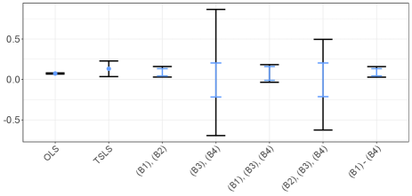
Figure 2: Two estimation strategies and five sensitivity models for the causal effect $\beta$: Point estimates/estimates of the PIR (blue); 95% confidence/sensitivity intervals (black).

Figure 2 shows the OLS and TSLS estimates as well as their corresponding 95% confidence intervals. The same plot shows the estimated partially identified regions and 95% sensitivity intervals (obtained by BCa bootstrap) for five different sensitivity models that involve different combinations of the bounds (B1) to (B4). Both the OLS and the TSLS estimates suggest a statistically significant positive effect of education on earnings. In the first sensitivity model in Figure 2, we relax the assumption of no unmeasured confounders, which would be required if the OLS estimate is interpreted causally, and assume that the effects of $U$ on $D$ and $Y$ are bounded by (B1) and (B2), respectively. In this case, the sensitivity interval remains positive. In other cases, the estimated partially identified regions and the sensitivity intervals become very wide whenever (B1) is not part of the constraints. Only specifying constraints on the IV sensitivity parameters, such as (B3) and (B4), is generally not sufficient to bound $\lvert R_{D\sim U|X,Z}\rvert$ away from 1. This is because the two regression and two IV sensitivity parameters only need to fulfill the equality constraint (8) leaving three degrees of freedom. In fact, if the loose bound (11) was not imposed, the PIR would have an infinite length and the association between $D$ and $Y$ may be entirely driven by the unmeasured confounder. Furthermore, we notice that adding the bound (B2) to (B3) and (B4) reduces the length of the sensitivity interval but yields the same estimated PIR. Since (B2) is a comparative bound and acts on both regression sensitivity parameters, similarly to (10), it depends on the specific dataset if (B2) actually bounds $\lvert R_{D\sim U|X,Z}\rvert$ away from 1. In the NLSYM data, (B2) does not accomplish this and we need to impose (11) to keep the length of the PIR finite.

Moreover, comparing the first and last sensitivity model in Figure 2, we notice that imposing the IV-related bounds (B3) and (B4) on top of (B1) and (B2) does not shorten the estimated PIR and sensitivity intervals. These findings suggest that the results of Card (1993) are more robust towards deviations from the OLS than from the IV assumptions.

6.2 Contour Plots

This subsection presents two graphical tools to further aid the interpretation of sensitivity analysis. The main idea is to plot the estimated lower or upper end of the PIR against the sensitivity parameters or the parameters in the comparative bounds. Contour lines in this plot allow practitioners to identify the magnitude of unmeasured confounding (or violations of the instrumental variables assumptions) needed to alter the conclusion of the study qualitatively. This idea dates back at least to Imbens (2003); our method below extends the proposal in Cinelli and Hazlett (2020). The contour plots will be illustrated using the real data example in the previous subsection.

6.2.1 $b$-contour Plot

For comparative bounds, the $b$-factor, such as $b_{U\!D}=4$ in (B1), controls how tightly the corresponding sensitivity parameter is constrained. Hence, it is important to gain a practical understanding of $b$. The $b$-sensitivity contour plot shows the estimated lower/upper end of the PIR on a grid of $b$-factors.

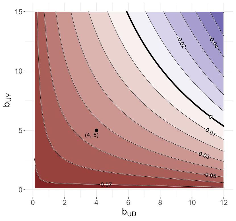
Figure 3: $b$-sensitivity contours for (B1), (B2).

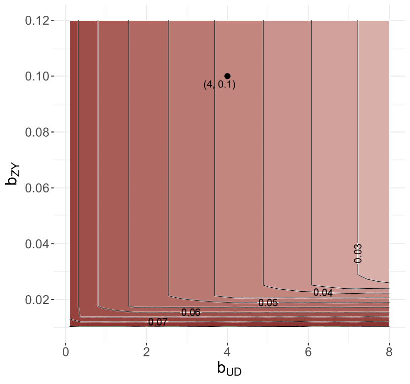
Figure 4: $b$-sensitivity contours for (B1)-(B4).

In Figure 3, we consider the sensitivity model with the bounds (B1) and (B2) and investigate our choice $(b_{U\!D},b_{UY})=(4,5)$. The plot shows that the estimated lower end of the PIR is still positive even for more conservative values such as $(b_{U\!D},b_{UY})=(6,10)$ or $(b_{U\!D},b_{UY})=(10,5)$. Thus, a substantial deviation from the OLS-related assumptions is needed to alter the sign of the estimate.

Figure 4 considers the sensitivity model using the constraints (B1) to (B4) with changing $(b_{U\!D},b_{ZY})$. This plot confirms our observation in Section 6.1 that imposing the IV-related bounds (B3) and (B4) does not change the estimated lower bound when (B1) and (B2) are already present. In the terminology of constrained optimization, this means that the “shadow prices” for (B3) and (B4) are small.

6.2.2 $R$-contour Plot

We may also directly plot the estimated lower/upper end of the PIR against the sensitivity parameters $R_{D\sim U|X,Z}$ and $R_{Y\sim U|X,Z,D}$. This idea has been adopted in several previous articles already (Imbens, 2003; Blackwell, 2014; Veitch and Zaveri, 2020).

For such $R$-contour plots, the key challenge is to benchmark or calibrate the partial $R$-values. This was often done informally by adding (multiples of) observed partial $R$-values to provide context for plausible values of the sensitivity parameters. Here, we build upon Cinelli and Hazlett (2020)’s contour plots and introduce rigorous benchmarking points using the comparative bounds on $U\rightarrow D$ and $U\rightarrow Y$. Since there are two comparative bounds on $U\rightarrow Y$, we also obtain two comparative values for $R_{Y\sim U|X,Z,D}$: one that does not condition on $D$ and one that does. The formulae for the comparison points can be found in Appendix 10 and the derivation in Section S6 of the Supplementary Materials.

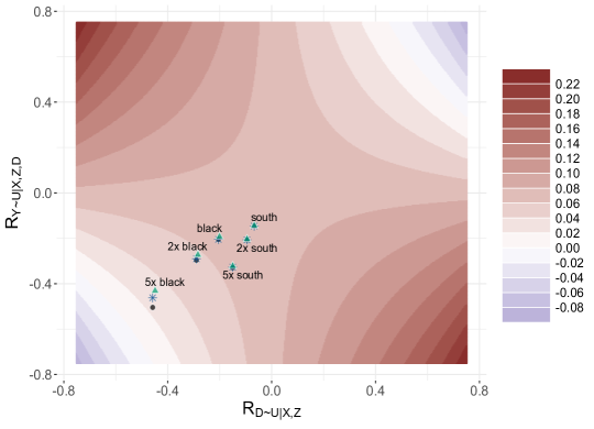
Figure 5: $R$-sensitivity contours for the lower end of the estimated PIR: Comparison points unconditional on $D$ (black dots), comparison points conditional on $D$ (blue stars) and non-rigorous comparison points (green triangles).

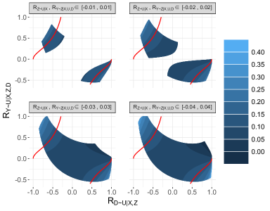
Figure 6: $R$-sensitivity contours for the lower end of the estimated PIR: The red lines correspond to the values of $R_{D\sim U|X,Z}$ and $R_{Y\sim U|X,Z,D}$ that conform with the IV-assumptions according to (8).

In Figure 5, we depict the $R$-contour plot for the estimated lower end of the PIR. To provide context for the values of $R_{D\sim U|X,Z}$ and $R_{Y\sim U|X,Z,D}$, we use the observed indicators for being black and living in the southern USA and add three different kinds of benchmarks each: our two proposed rigorous comparison points (unconditional and conditional on $D$) and an informal comparison point following Imbens’ proposal. We notice that, even if the unmeasured confounder was five times as strong as being black in terms of its capability of explaining the variation of $D$ and $Y$, the estimator would still be positive. This holds true regardless of whether the comparison for the effect of $U$ on $Y$ was made conditional or unconditional on $D$. Moreover, Figure 5 shows that the informal comparison point yields a similar result. In our experience, the difference between the methods usually does not change the qualitative conclusion of the sensitivity analysis.

Finally, we illustrate the utility of the $R$-contour plot as a way to visualize the feasible set $\Psi(\theta)$. Sensitivity analysis with multiple bounds often entails a complex set of constraints. Consider the following sensitivity model

$$R_{Z\sim U|X},\,R_{Y\sim Z|X,U,D}\in[-r,r],\quad r\in\{0.01,0.02,0.03,0.04\},$$

$$R^{2}_{Y\sim U|\tilde{X},\dot{X}_{-j},Z,D}\leq 5\,R^{2}_{Y\sim\dot{X}_{j}|\tilde{X},\dot{X}_{-j},Z,D},\qquad R_{D\sim U|X,Z}\in[-0.99,0.99],$$

where $r$ parameterizes the degree of deviation from the instrumental variables assumptions and the covariate $\dot{X}_{j}$ is the indicator for being black.

Figure 6 shows the estimated feasible set $\Psi(\hat{\theta})$ for different values of $r$. For $r=0.01$, the feasible set is small and concentrated around the lines that correspond to $R_{D\sim U|X,Z}=R_{Y\sim U|X,Z,D}=0$ (the instrumental variable is valid). As $r$ increases, the feasible set becomes larger as expected. The curved shape of the region of feasible values is a result of the comparative bound on $U\rightarrow Y$ and the associated constraints. Moreover, we observe that $\beta$ assumes its most extreme values as $R_{D\sim U|X,Z}$ approaches 1. This highlights the importance of bounding $R_{D\sim U|X,Z}$ away from $-1$ and $1$ to ensure that the PIR has finite length.

7 Discussion and Outlook

The methodological developments in this article are underpinned by two insights. First, sensitivity analysis (or more generally, any one-dimensional partially identified problem) may be viewed as a constrained stochastic program and we can leverage methods developed in stochastic optimization. Second, the $R^{2}$-calculus provides a parameterization of the linear causal effect and a systematic approach to specify interpretable sensitivity models.

Partial identification has attracted considerable attention in econometrics and causal inference since the work of Manski (1990) and Balke and Pearl (1997); for instance Manski (2003); Imbens and Manski (2004); Vansteelandt et al. (2006); Chernozhukov et al. (2007); Aronow and Lee (2013); Richardson et al. (2014); Miratrix et al. (2018); Molinari (2020). Existing methods typically assume a closed-form solution to the stochastic program (2) (the lower/upper end of the PIR) and that the plug-in estimator is asymptotically normal. As such results are only known for relatively simple models, these methods only have limited utility in practice. The constrained optimization perspective of partial identification is only beginning to get embraced in the literature (Kaido et al., 2019; Hu et al., 2021; Guo et al., 2022; Padh et al., 2023).

Our article further shows the need for a more complete, asymptotic theory of the optimal value of a general stochastic program. This may allow us to extend the methodology developed here to sensitivity models with high- or infinite-dimensional parameters. In particular, a theory for the bootstrap distribution of the optimal value estimator is required to clarify when and which bootstrap procedures provide asymptotically valid sensitivity intervals.

The $R^{2}$-values, $R$-values and generalizations thereof are popular for the calibration of sensitivity analysis. Recently, they have been used for linear models with multiple treatments (Zheng et al., 2021), mediation analysis (Zhang and Ding, 2022), missing values (Colnet et al., 2022) and models with factor-structured outcomes (Zheng et al., 2023). In these works, certain algebraic relationships about $R^{2}$-values and benchmarking techniques such as contour plots and robustness values are frequently used. Thus, the methodology developed in this article may also benefit the calibration of other sensitivity models. Moreover, our proof of the $R^{2}$-calculus in general Hilbert spaces – see Supplementary Material S1 – suggests that it may be useful in nonlinear models, too. See Chernozhukov et al. (2022) for related work in partially linear and semiparametric models using the Riesz-Frechet representation of certain causal parameters.

The rules of the $R^{2}$-calculus are purely algebraic and can therefore be applied whenever a (causal) effect is defined in terms of a covariance matrix – regardless of the number of observed and unobserved variables. This raises the question: can sensitivity analysis be automated for reasonable sensitivity models defined by direct and comparative bounds? Such an algorithm would be immensely useful in applied research, but given the substantial amount of algebra needed for the relatively simple models considered here, the required work would be rather challenging.

8 R²-Calculus

Going forward, we use the notation of Section 2.1, only state results for the population versions of the (partial) $R$- and $R^{2}$-values and assume without loss of generality that random variables are centred.

The following result justifies calling $R^{2}_{Y\sim X\mid Z}$ a partial $R^{2}$-value and shows that the definitions of $R^{2}$- and $R$-value are consistent. It follows from the Gram-Schmidt orthogonalization.

Lemma 3.

In the setting of Definition 1, $R^{2}_{Y\sim X|Z}=R^{2}_{Y^{\perp Z}\sim X^{\perp Z}}$. Moreover, if $X$ is one-dimensional, then $R^{2}_{Y\sim X|Z}=(R_{Y\sim X|Z})^{2}$.

Partial $R$- and $R^{2}$-values that involve overlapping sets of random variables need fulfill certain algebraic relationships. These can be used to identify the causal effect $\beta$ in terms of sensitivity parameters and derive interpretable constraints. The next Proposition collects several useful algebraic rules we harness in this article.

Proposition 4 ($R^{2}$-calculus).

In the setting of Definition 1, assume that $W$ is another random vector such that the covariance matrix of $(Y,X,Z,W)$ is positive definite. Then, the following algebraic rules hold:

• Orthogonality: if $\operatorname*{corr}(Y,X_{i})=0$ for all components $i$ of $X$, then $R^{2}_{Y\sim X}=0$;

• Orthogonal additivity: if $R^{2}_{X_{i}\sim W}=0$ for all components $i$ of $X$, then

  $$R^{2}_{Y\sim X+W}=R^{2}_{Y\sim X}+R^{2}_{Y\sim W};$$

• Decomposition of unexplained variance:

  $$1-R^{2}_{Y\sim X+W}=(1-R^{2}_{Y\sim X})(1-R^{2}_{Y\sim W|X});$$

• Recursion of partial correlation: if $X$ and $W$ are one-dimensional, then

  $$R_{Y\sim X|W}=\frac{R_{Y\sim X}-R_{Y\sim W}R_{X\sim W}}{\sqrt{1-R_{Y\sim W}^{2}}\sqrt{1-R^{2}_{X\sim W}}};$$

• Reduction of partial correlation: if $X$ is one-dimensional and $R^{2}_{Y\sim W}=0$, then

  $$R_{Y\sim X|W}=\frac{R_{Y\sim X}}{\sqrt{1-R^{2}_{X\sim W}}};$$

• Three-variable identity: if both $X$ and $W$ are one-dimensional, then

  $$f_{Y\sim X|W}\sqrt{1-R^{2}_{Y\sim W|X}}=f_{Y\sim X}\sqrt{1-R^{2}_{X\sim W}}-R_{Y\sim W|X}R_{X\sim W}.$$

All of the relationships above also hold when $Z$ is partialed out, i.e. if “ $|Z$” is appended to the subscripts of all $R$-, $R^{2}$-, and $f$-values and $Z$ is partialed out in the correlations.

Remark 4.

Rule [vi] may appear unintuitive at first. To see how this identity may come up, consider three random variables $Y$, $X$ and $W$. There are in total three marginal $R$-values, $R_{Y\sim X}$, $R_{Y\sim W}$ and $R_{X\sim W}$, and three partial $R$-values, $R_{Y\sim X|W}$, $R_{Y\sim W|X}$ and $R_{X\sim W|Y}$. Rule [iv] shows that the partial $R$-values can be determined by all the marginal values. In other words, there are only three degrees of freedom among the six $R$-values. This implies that there must be an equality constraint relating $R_{Y\sim X}$, $R_{X\sim W}$, $R_{Y\sim X|W}$, and $R_{Y\sim W|X}$.

In general, a conditional independence statement such as $Y\perp\kern-5.38193pt\perp W\,|\,X$ does not imply that $Y$ and $W$ are partially uncorrelated given $X$. However, if the conditional expectation of $Y$ and $W$ is affine linear in $X$, $\operatorname*{corr}(Y^{\perp X},W^{\perp X})=0$ indeed holds true (Baba et al., 2004, Thm. 1). Hence, if we assume that $(Y,X,Z,D,U)$ follow a linear structural equation model, we could replace the assumptions in rules [i], [ii] and [v] with corresponding (conditional) independence statements. For more details on the relationship of partial correlation, conditional correlation and conditional independence, we refer to Baba et al. (2004).

The (partial) $R^{2}$- and $R$-value can be defined in a more general Hilbert space setting. The corresponding rules of the $R^{2}$-calculus also hold true, yielding Proposition 4 as a corollary. We refer the reader to Section S1 of the Supplementary Material for more details.

9 Details on the Sensitivity Model

9.1 Relationship between Regression and IV Sensitivity Parameters

In order to derive the equality constraint (8), we apply the three-variable identity from the $R^{2}$-calculus twice: First, we set $Y\equiv Y$, $X\equiv Z$, $W\equiv U$ and $Z\equiv(X,D)$; second, $Y\equiv U$, $X\equiv Z$, $W\equiv D$ and $Z\equiv X$. This yields

$$f_{Y\sim Z|X,U,D}\sqrt{1-R^{2}_{Y\sim U|X,Z,D}} =f_{Y\sim Z|X,D}\sqrt{1-R^{2}_{Z\sim U|X,D}}-R_{Y\sim U|X,Z,D}R_{Z\sim U|X,D},$$

$$f_{Z\sim U|X,D}\sqrt{1-R^{2}_{D\sim U|X,Z}} =f_{Z\sim U|X}\sqrt{1-R^{2}_{D\sim Z|X}}-R_{D\sim Z|X}R_{D\sim U|X,Z}.$$

This constraint suffices to recover point-identification of $\beta$ if $Z$ is a valid instrument. Indeed, if we set $R_{Z\sim U|X}=0$ and $R_{Y\sim Z|X,U,D}=0$ in the equations above and simplify them, we get the relationship

$$f_{D\sim U|X,Z}\,R_{Y\sim U|X,Z,D}=-\frac{f_{Y\sim Z|X,D}}{R_{D\sim Z|X}}.$$

Plugging this result into equation (5), we directly obtain $\beta=\beta_{D\sim Z|X,Y\sim Z|X}$.

9.2 Optimization Constraints

Table 2: Equality and inequality constraints stemming from comparative bounds.

Edge	Optimization constraint
	$\displaystyle R^{2}_{D\sim U|X,Z}\leq b_{U\!D}\frac{R^{2}_{D\sim\dot{X}_{J}|\tilde{X},\dot{X}_{I},Z}}{1-R^{2}_{D\sim\dot{X}_{I^{c}}|\tilde{X},\dot{X}_{I},Z}}$	(12)eq:reg-cond-d2
	$\displaystyle R_{Y\sim U|X,Z,D}=\frac{R_{Y\sim U|X,Z}-R_{Y\sim D|X,Z}\,R_{D\sim U|X,Z}}{\sqrt{1-R^{2}_{Y\sim D|X,Z}}\sqrt{1-R^{2}_{D\sim U|X,Z}}}$	(13)eq:reg-con-y22
	$\displaystyle R^{2}_{Y\sim U|X,Z}\leq b_{UY}\frac{R^{2}_{Y\sim\dot{X}_{J}|\tilde{X},\dot{X}_{I},Z}}{1-R^{2}_{Y\sim\dot{X}_{I^{c}}|\tilde{X},\dot{X}_{I},Z}}$	(14)eq:reg-con-y21
	$\begin{multlined}R_{Y\sim U|X,Z}=\frac{1}{\sqrt{1-R^{2}_{Y\sim\dot{X}_{I^{c}}|\tilde{X},\dot{X}_{I},Z}}}\bigg{[}R_{Y\sim D|\tilde{X},\dot{X}_{I},Z}R_{D\sim U|X,Z}\sqrt{1-R^{2}_{D\sim\dot{X}_{I^{c}}|\tilde{X},\dot{X}_{I},Z}}\\[-17.22217pt] +R_{Y\sim U|\tilde{X},\dot{X}_{I},Z,D}\sqrt{1-R^{2}_{Y\sim D|\tilde{X},\dot{X}_{I},Z}}\sqrt{1-R^{2}_{D\sim U|X,Z}(1-R^{2}_{D\sim\dot{X}_{I^{c}}|\tilde{X},\dot{X}_{I},Z})}\bigg{]}\end{multlined}R_{Y\sim U|X,Z}=\frac{1}{\sqrt{1-R^{2}_{Y\sim\dot{X}_{I^{c}}|\tilde{X},\dot{X}_{I},Z}}}\bigg{[}R_{Y\sim D|\tilde{X},\dot{X}_{I},Z}R_{D\sim U|X,Z}\sqrt{1-R^{2}_{D\sim\dot{X}_{I^{c}}|\tilde{X},\dot{X}_{I},Z}}\\[-17.22217pt] +R_{Y\sim U|\tilde{X},\dot{X}_{I},Z,D}\sqrt{1-R^{2}_{Y\sim D|\tilde{X},\dot{X}_{I},Z}}\sqrt{1-R^{2}_{D\sim U|X,Z}(1-R^{2}_{D\sim\dot{X}_{I^{c}}|\tilde{X},\dot{X}_{I},Z})}\bigg{]}$	(15)eq:reg-con-y32
	$\displaystyle R^{2}_{Z\sim U|X}\leq b_{U\!Z}\,R^{2}_{Z\sim\dot{X}_{j}|\tilde{X},\dot{X}_{-j}}\frac{1-R^{2}_{Z\sim\dot{X}_{j}|\tilde{X},\dot{X}_{-j}}}{1-b_{U\!Z}\,R^{4}_{Z\sim\dot{X}_{j}|\tilde{X},\dot{X}_{-j}}}$	(16)eq:iv-con-z2
	$\displaystyle\begin{multlined}f_{Y\sim\dot{X}_{j}|\tilde{X},\dot{X}_{-j},Z,U,D}\sqrt{1-R^{2}_{Y\sim U|X,Z,D}}=\bigg{[}f_{Y\sim\dot{X}_{j}|\tilde{X},\dot{X}_{-j},Z,D}\sqrt{1-R^{2}_{D\sim U|X,Z}}\\[-17.22217pt] +R_{Y\sim U|X,Z,D}\,R_{D\sim\dot{X}_{j}|\tilde{X},\dot{X}_{-j},Z}\,R_{D\sim U|X,Z}\bigg{]}\Big{/}\sqrt{1-R^{2}_{D\sim U|X,Z}(1-R^{2}_{D\sim\dot{X}_{j}|\tilde{X},\dot{X}_{-j},Z})}\end{multlined}f_{Y\sim\dot{X}_{j}|\tilde{X},\dot{X}_{-j},Z,U,D}\sqrt{1-R^{2}_{Y\sim U|X,Z,D}}=\bigg{[}f_{Y\sim\dot{X}_{j}|\tilde{X},\dot{X}_{-j},Z,D}\sqrt{1-R^{2}_{D\sim U|X,Z}}\\[-17.22217pt] +R_{Y\sim U|X,Z,D}\,R_{D\sim\dot{X}_{j}|\tilde{X},\dot{X}_{-j},Z}\,R_{D\sim U|X,Z}\bigg{]}\Big{/}\sqrt{1-R^{2}_{D\sim U|X,Z}(1-R^{2}_{D\sim\dot{X}_{j}|\tilde{X},\dot{X}_{-j},Z})}$	(17)eq:iv-con-ex22

In Table 1, we list different sensitivity bounds that practitioners can specify. For direct constraints, practitioners need to specify a lower and an upper bound – $B^{l}$ and $B^{u}$ – on the values of the respective sensitivity parameters. For comparative constraints, they choose a comparison random variable (or group of random variables) and specify a positive number $b$ that relates the explanatory capability of $U$ to the chosen variable(s). While we can immediately add direct sensitivity bounds to the constraints of the optimization problem, we need to reformulate comparative bounds and possibly add equality constraints to relate them to the regression and IV sensitivity parameters. Table 2 lists these optimization constraints emerging from the comparative bounds in Table 1. The derivations of the respective equalities and inequalities can be found in Supplementary Material S3.

If only constraints on $U\rightarrow D$ and $U\rightarrow Y$ are given, the user-specified sensitivity bounds in Table 1 and (additional) optimization constraints in Table 2 can all be reformulated as bounds on the two sensitivity parameters $R_{Y\sim U|X,Z,D}$ and $R_{D\sim U|X,Z}$; this can be seen by substituting the equality into the inequality constraints. Hence, the resulting sensitivity model has two degrees of freedom. Similarly, if additionally constraints on $U\leftrightarrow U$ and/or $Z\rightarrow Y$ are specified, the sensitivity model can be parameterized in terms of $R_{Y\sim U|X,Z,D}$, $R_{D\sim U|X,Z}$ and $R_{Z\sim U|X}$ and is thus three-dimensional.

In practice, we work with the formulation involving equality constraints and additional unestimable parameters, such as $R_{Y\sim U|X,Z}$, to keep the the algebraic expressions tractable. In spirit, this is similar to the use of slack variables in optimization.

10 R-contour Plot – Comparison Points

In Section 6.2.2, we consider three different kinds of comparison points. The first approach follows a proposal by Imbens and adds the points

$$\left(\sqrt{b}\,\hat{R}_{D\sim X_{j}|X_{-j},Z},\,\sqrt{b}\,\hat{R}_{Y\sim X_{j}|X_{-j},Z,D}\right),$$

for certain choices of $b>0$ and $j\in[p]$ to the contour plot. However, this method of constructing benchmarks for $R_{D\sim U|X,Z}$ and $R_{Y\sim U|X,Z,D}$ is not entirely honest because different sets of covariates are conditioned on. Moreover, regressing out a potential collider $D$ may leave $\hat{R}^{2}_{Y\sim X_{j}|X_{-j},Z,D}$ hard to interpret.

Therefore, we derive rigorous comparison points. To this end, we introduce the abbreviations

$$\hat{R}_{D}:=\hat{R}_{D\sim\dot{X}_{j}|\tilde{X},\dot{X}_{-j},Z},\qquad\hat{R}_{Y}:=\hat{R}_{Y\sim\dot{X}_{j}|\tilde{X},\dot{X}_{-j},Z,D},$$

where $j\in[\dot{p}]$; the corresponding $\hat{R}^{2}$- and $\hat{f}$-values are defined accordingly.

First, we consider the sensitivity parameter $R_{D\sim U|X,Z}$. Due to (2), if $U$ explains $b$ times as much variance of $D$ as $\dot{X}_{j}$ and the respective correlations of $U$ and $\dot{X}_{j}$ with $D$ have the same sign, then

$$R_{D\sim U|X,Z}=\sqrt{b}\,\frac{R_{D\sim\dot{X}_{j}|\tilde{X},\dot{X}_{-j},Z}}{\sqrt{1-R^{2}_{D\sim\dot{X}_{j}|\tilde{X},\dot{X}_{-j},Z}}}=\sqrt{b}\,f_{D\sim\dot{X}_{j}|\tilde{X},\dot{X}_{-j},Z}.$$ (18)

For the second sensitivity parameter $R_{Y\sim U|X,Z,D}$, we can make two types of comparisons: unconditional and conditional on $D$, cf. sensitivity bounds on $U\rightarrow Y$ in Table 1. In the former case, we assume that $U$ explains $b$ times as much variance in $Y$ as $\dot{X}_{j}$ does, given $(\tilde{X},\dot{X}_{-j},Z)$, and that the respective correlations have the same sign. In the latter case, we additionally condition on $D$. For the first comparison, using the relationships (2) and (2) yields

$$R_{Y\sim U|X,Z,D}=\frac{1}{\sqrt{1-(1+b)R^{2}_{D\sim\dot{X}_{j}|\tilde{X},\dot{X}_{-j},Z}}}\,\sqrt{b}\,f_{Y\sim\dot{X}_{j}|\tilde{X},\dot{X}_{-j},Z,D}.$$ (19)

For the second comparison, we apply a similar reasoning and obtain

$$R_{Y\sim U|X,Z,D}=\frac{\sqrt{1-(1+b)R_{D\sim\dot{X}_{j}|\tilde{X},\dot{X}_{-j},Z}^{2}\!+bR_{D\sim\dot{X}_{j}|\tilde{X},\dot{X}_{-j},Z}^{4}}\!+\!R_{D\sim\dot{X}_{j}|\tilde{X},\dot{X}_{-j},Z}^{2}}{\sqrt{1-(1+b)R^{2}_{D\sim\dot{X}_{j}|\tilde{X},\dot{X}_{-j},Z}}}\,\sqrt{b}\,f_{Y\sim\dot{X}_{j}|\tilde{X},\dot{X}_{-j},Z,D}.$$ (20)

The derivations can be found in the Supplementary Material S6. In order to compare $U$ to $b$ times the explanatory capability of $\dot{X}_{j}$, we can add the estimated comparison points

$$\left(\sqrt{b}\hat{f}_{D},\,\frac{1}{\sqrt{1-(1+b)\hat{R}_{D}^{2}}}\,\sqrt{b}\,\hat{f}_{Y}\right),\quad\text{or}\quad\left(\sqrt{b}\hat{f}_{D},\,\frac{\sqrt{1-(1+b)\hat{R}_{D}^{2}+b\hat{R}_{D}^{4}}+\hat{R}_{D}^{2}}{\sqrt{1-(1+b)\hat{R}_{D}^{2}}}\,\sqrt{b}\,\hat{f}_{Y}\right),$$

depending on whether we compare $U$ and $\dot{X}_{j}$ unconditional or conditional on $D$. The corresponding comparison points for $R^{2}$- instead of $R$-values were suggested by Cinelli and Hazlett (2020). Moreover, we remark that the two proposed points are identical if $b=1$.

Competing interests

No competing interest is declared.

S1 Hilbert Space R²-Calculus and Proofs

The algebraic rules of the $R^{2}$-calculus – both the population version in Proposition 4 and its sample counterpart – are not specific to linear models. In fact, all relationships fundamentally stem from the geometry of projections in Hilbert spaces. For this reason, the definitions of $R^{2}$- and $R$-values can be generalized and the corresponding algebraic rules be proven in more generality.

This section is organized as follows. First, we recall some results on Hilbert space theory (Halmos, 2000, sec. 26-29) and define generalized (partial) $R^{2}$- and $R$-values. Then, we prove Hilbert space generalizations to Lemma 3 and Proposition 4. Finally, in Section S1.3, we explain how the $R^{2}$-calculus for linear models directly follows from these results and provide more details on the assumptions and notation involved.

S1.1 Hilbert Space R²-value

Let $(\mathcal{H},\langle\cdot,\cdot\rangle)$ be a Hilbert space over the field $\mathbb{K}$ of real or complex numbers; denote its associated norm as $\lVert\cdot\rVert$ and let $\mathcal{X},\mathcal{Y},\mathcal{Z}\subseteq\mathcal{H}$ be closed linear subspaces. The Minkowski sum of $\mathcal{Y}$ and $\mathcal{X}$ is given by $\mathcal{X}+\mathcal{Y}:=\{x+y\colon x\in\mathcal{X},y\in\mathcal{Y}\}$. For $x\in\mathcal{X}$ and $y\in\mathcal{Y}$, we write $x\perp y$, if $\langle x,y\rangle=0$, $x\perp\mathcal{Y}$, if $x\perp y$ for all $y\in\mathcal{Y}$, and $\mathcal{X}\perp\mathcal{Y}$, if $x\perp\mathcal{Y}$ for all $x\in\mathcal{X}$. For every element $h\in\mathcal{H}$, there are unique $x\in\mathcal{X}$ and $x^{\perp}\in\mathcal{H}$ such that $x\perp x^{\perp}$ and $h=x+x^{\perp}$.

Definition S1.

The projection on $\mathcal{X}$ is the operator $P_{\mathcal{X}}\colon\mathcal{H}\to\mathcal{X}$ defined by the assignment ${h=x+x^{\perp}\mapsto x}$. The projection off $\mathcal{X}$ is the operator $Q_{\mathcal{X}}\colon\mathcal{H}\to\mathcal{H}$ defined by ${h=x+x^{\perp}\mapsto x^{\perp}}$.

Clearly, the projection on and off $\mathcal{X}$ add up to the identity operator, i.e. $P_{\mathcal{X}}+Q_{\mathcal{X}}=\mathrm{Id}$. Furthermore, we introduce the notations $y^{\perp\mathcal{X}}:=Q_{\mathcal{X}}\,y$ and $\mathcal{Y}^{\perp\mathcal{X}}:=\{y^{\perp\mathcal{X}}\colon{y\in\mathcal{Y}}\}$. The space $\mathcal{Y}^{\perp\mathcal{X}}$ is a closed linear subspace of $\mathcal{H}$; thus, the projections $P_{\mathcal{Y}^{\perp\mathcal{X}}}$ and $Q_{\mathcal{Y}^{\perp\mathcal{X}}}$ are well-defined. They can be used to define conditional orthogonality: $\mathcal{Y}\perp\mathcal{X}\,|\,\mathcal{Z}\Leftrightarrow\mathcal{Y}^{\perp\mathcal{Z}}\perp\mathcal{X}^{\perp\mathcal{Z}}$.

Lemma S1.

hello

• $P_{\mathcal{X}}$ and $Q_{\mathcal{X}}$ are linear, self-adjoint, and idempotent operators.

• If $\mathcal{X}\perp\mathcal{Y}$, $P_{\mathcal{X}+\mathcal{Y}}=P_{\mathcal{X}}+P_{\mathcal{Y}}$ and $Q_{\mathcal{X}+\mathcal{Y}}=Q_{\mathcal{X}}\,Q_{\mathcal{Y}}$.

• $P_{\mathcal{X}+\mathcal{Y}}=P_{\mathcal{X}}+P_{\mathcal{Y}^{\perp\mathcal{X}}}$ and $Q_{\mathcal{X}+\mathcal{Y}}=Q_{\mathcal{X}}\,Q_{\mathcal{Y}^{\perp\mathcal{X}}}=Q_{\mathcal{Y}^{\perp\mathcal{X}}}\,Q_{\mathcal{X}}$.

• If $h_{1},h_{2}\in\mathcal{H}$ and $h_{1}\perp h_{2}$, $\lVert h_{1}+h_{2}\rVert^{2}=\lVert h_{1}\rVert^{2}+\lVert h_{2}\rVert^{2}$.

Proof.

hello

• See Halmos (2000, sec. 26, Thm. 1).

• See Halmos (2000, sec. 28, Thm. 2) for the proof of $P_{\mathcal{X}+\mathcal{Y}}=P_{\mathcal{X}}+P_{\mathcal{Y}}$. According to Halmos (2000, sec. 29, Thm. 1), $P_{\mathcal{X}}P_{\mathcal{Y}}=0$ holds due to $\mathcal{X}\perp\mathcal{Y}$. Hence, the second statement directly follows: $Q_{\mathcal{X}+\mathcal{Y}}=\mathrm{Id}-P_{\mathcal{X}}-P_{\mathcal{Y}}=(\mathrm{Id}-P_{\mathcal{X}})(\mathrm{Id}-P_{\mathcal{Y}})=Q_{\mathcal{X}}\,Q_{\mathcal{Y}}$.

• We rewrite the direct sum $\mathcal{X}+\mathcal{Y}$ as follows

  $$\mathcal{X}+\mathcal{Y} =\{x+y\colon x\in\mathcal{X},y\in\mathcal{Y}\}=\{x+P_{\mathcal{X}}\,y+Q_{\mathcal{X}}\,y\colon x\in\mathcal{X},y\in\mathcal{Y}\}$$

  $$=\{x+Q_{\mathcal{X}}\,y\colon x\in\mathcal{X},y\in\mathcal{Y}\}=\mathcal{X}+\mathcal{Y}^{\perp\mathcal{X}}.$$

  Since $\mathcal{X}$ and $\mathcal{Y}^{\perp\mathcal{X}}$ are orthogonal by definition, the result directly follows from (ii).

• See Halmos (2000, sec. 4, Thm. 3). ∎

Any one-dimensional linear subspace $\mathcal{X}$ can be expressed as $\mathcal{X}=\{\lambda\,x\colon\lambda\in\mathbb{K}\}$, where $x$ is an arbitrary element in $\mathcal{X}\setminus\{0\}$. Hence, we can identify a one-dimensional subspace with any non-zero element contained in it.

Definition S2 (Hilbert space $R^{2}$- and $R$-value).

Let $\mathcal{X},\mathcal{Y},\mathcal{Z}\subseteq\mathcal{H}$ be closed linear subspaces. Assume $\mathcal{Y}$ is one-dimensional, let $y\in\mathcal{Y}\setminus\{0\}$ and suppose $\lVert y^{\perp\mathcal{Z}}\rVert^{2}>0$. The (marginal) $R^{2}$-value of $\mathcal{Y}$ on $\mathcal{X}$, the partial $R^{2}$-value of $\mathcal{Y}$ on $\mathcal{X}$ given $\mathcal{Z}$ and the partial $f^{2}$-value of $\mathcal{Y}$ on $\mathcal{X}$ given $\mathcal{Z}$ are defined as

$$R^{2}_{\mathcal{Y}\sim\mathcal{X}}:=1-\frac{\lVert y^{\perp\mathcal{X}}\rVert^{2}}{\lVert y\rVert^{2}},\qquad R^{2}_{\mathcal{Y}\sim\mathcal{X}|\mathcal{Z}}:=\frac{R^{2}_{\mathcal{Y}\sim\mathcal{X}+\mathcal{Z}}-R^{2}_{\mathcal{Y}\sim\mathcal{Z}}}{1-R^{2}_{\mathcal{Y}\sim\mathcal{Z}}},\qquad f^{2}_{\mathcal{Y}\sim\mathcal{X}|\mathcal{Z}}:=\frac{R^{2}_{\mathcal{Y}\sim\mathcal{X}|\mathcal{Z}}}{1-R^{2}_{\mathcal{Y}\sim\mathcal{X}|\mathcal{Z}}},$$

respectively. If $\mathcal{X}$ is one-dimensional, $x\in\mathcal{X}\setminus\{0\}$ and $\lVert x^{\perp\mathcal{Z}}\rVert^{2}>0$, the partial $R$- and $f$-value are given by

$$R_{\mathcal{Y}\sim\mathcal{X}|\mathcal{Z}}:=\frac{\langle y^{\perp\mathcal{Z}},x^{\perp\mathcal{Z}}\rangle}{\lVert y^{\perp\mathcal{Z}}\rVert\,\lVert x^{\perp\mathcal{Z}}\rVert},\qquad f_{\mathcal{Y}\sim\mathcal{X}|\mathcal{Z}}:=\frac{R_{\mathcal{Y}\sim\mathcal{X}|\mathcal{Z}}}{\sqrt{1-R_{\mathcal{Y}\sim\mathcal{X}|\mathcal{Z}}^{2}}}.$$

The choice of the non-zero elements $y$ and $x$ does not change the (partial) $R^{2}$- and $R$-values due to the normalization. Therefore, all quantities above are well-defined.

S1.2 Proofs of Results in Appendix 8

In this subsection, we state and prove the generalized versions of Lemma 3 and Proposition 4.

Lemma S2.

In the setting of Definition S2, $R^{2}_{\mathcal{Y}\sim\mathcal{X}|\mathcal{Z}}=R^{2}_{\mathcal{Y}^{\perp\mathcal{Z}}\sim\mathcal{X}^{\perp\mathcal{Z}}}$ holds true. Moreover, if $\mathcal{X}$ is a one-dimensional subspace, then $R^{2}_{\mathcal{Y}\sim\mathcal{X}|\mathcal{Z}}=(R_{\mathcal{Y}\sim\mathcal{X}|\mathcal{Z}})^{2}$.

Proof.

The first statement of the lemma follows from some elementary algebraic manipulations and applying Lemma S1 (iii):

$$R^{2}_{\mathcal{Y}\sim\mathcal{X}|\mathcal{Z}} =\frac{R^{2}_{\mathcal{Y}\sim\mathcal{X}+\mathcal{Z}}-R^{2}_{\mathcal{Y}\sim\mathcal{Z}}}{1-R^{2}_{\mathcal{Y}\sim\mathcal{Z}}}\left[1-\frac{\lVert y^{\perp\mathcal{X}+\mathcal{Z}}\rVert^{2}}{\lVert y\rVert^{2}}-1+\frac{\lVert y^{\perp\mathcal{Z}}\rVert^{2}}{\lVert y\rVert^{2}}\right]\bigg{/}\frac{\lVert y^{\perp\mathcal{Z}}\rVert^{2}}{\lVert y\rVert^{2}}$$

$$=1-\frac{\lVert y^{\perp\mathcal{X}+\mathcal{Z}}\rVert^{2}}{\lVert y^{\perp\mathcal{Z}}\rVert^{2}}\stackrel{{\scriptstyle\text{(iii)}}}{{=}}1-\frac{\lVert Q_{\mathcal{X}^{\perp\mathcal{Z}}}\,y^{\perp\mathcal{Z}}\rVert^{2}}{\lVert y^{\perp\mathcal{Z}}\rVert^{2}}=R^{2}_{\mathcal{Y}^{\perp\mathcal{Z}}\sim\mathcal{X}^{\perp\mathcal{Z}}}.$$

To prove the second part of the lemma, we assume that $\mathcal{X}$ is one-dimensional and choose $x\in\mathcal{X}\setminus\{0\}$. If $\mathcal{X}^{\perp\mathcal{Z}}=0$, the projection on $\mathcal{X}^{\perp\mathcal{Z}}$ is 0; otherwise, it is given by

$$P_{\mathcal{X}^{\perp\mathcal{Z}}}h=\frac{\langle h,x^{\perp\mathcal{Z}}\rangle x^{\perp\mathcal{Z}}}{\lVert x^{\perp\mathcal{Z}}\rVert^{2}},\quad\text{for }h\in H.$$ (S1)

This can be easily checked: $P_{\mathcal{X}^{\perp\mathcal{Z}}}$ is linear and its image is contained in $\mathcal{X}^{\perp\mathcal{Z}}$. Moreover,

$$\bigg{\langle}\frac{\langle h,x^{\perp\mathcal{Z}}\rangle\,x^{\perp\mathcal{Z}}}{\lVert x^{\perp\mathcal{Z}}\rVert^{2}},\,h-\frac{\langle h,x^{\perp\mathcal{Z}}\rangle\,x^{\perp\mathcal{Z}}}{\lVert x^{\perp\mathcal{Z}}\rVert^{2}}\bigg{\rangle}=\frac{\langle h,x^{\perp\mathcal{Z}}\rangle^{2}}{\lVert x^{\perp\mathcal{Z}}\rVert^{2}}-\frac{\langle h,x^{\perp\mathcal{Z}}\rangle^{2}\lVert x^{\perp\mathcal{Z}}\rVert^{2}}{\lVert x^{\perp\mathcal{Z}}\rVert^{4}}=0.$$

Following from the first part of the proof and Lemma S1 (iv), we infer

$$R^{2}_{\mathcal{Y}\sim\mathcal{X}|\mathcal{Z}}=1-\frac{\lVert Q_{\mathcal{X}^{\perp\mathcal{Z}}}\,y^{\perp\mathcal{Z}}\rVert^{2}}{\lVert y^{\perp\mathcal{Z}}\rVert^{2}}\stackrel{{\scriptstyle\text{(iv)}}}{{=}}\frac{\lVert P_{\mathcal{X}^{\perp\mathcal{Z}}}\,y^{\perp\mathcal{Z}}\rVert^{2}}{\lVert y^{\perp\mathcal{Z}}\rVert^{2}}.$$

Inserting the formula for the projection on $\mathcal{X}^{\perp\mathcal{Z}}$ yields the second statement of the lemma

$$R^{2}_{\mathcal{Y}\sim\mathcal{X}|\mathcal{Z}}=\frac{\lVert\langle y^{\perp\mathcal{Z}},x^{\perp\mathcal{Z}}\rangle\,x^{\perp\mathcal{Z}}\rVert^{2}}{\lVert y^{\perp\mathcal{Z}}\rVert^{2}\,\lVert x^{\perp\mathcal{Z}}\rVert^{4}}=\frac{\langle y^{\perp\mathcal{Z}},x^{\perp\mathcal{Z}}\rangle^{2}\rVert x^{\perp\mathcal{Z}}\rVert^{2}}{\lVert y^{\perp\mathcal{Z}}\rVert^{2}\,\lVert x^{\perp\mathcal{Z}}\rVert^{4}}=\big{(}R_{\mathcal{Y}\sim\mathcal{X}|\mathcal{Z}}\big{)}^{2}.\hfill\qed$$

Proposition S3 (Hilbert space $R^{2}$-calculus).

In the setting of Definition S2, let $\mathcal{W}$ be another closed linear subspace. Assume $\lVert\mathcal{Y}^{\perp\mathcal{X}+\mathcal{W}+\mathcal{Z}}\rVert^{2}>0$. Further suppose ${\lVert\mathcal{X}^{\perp\mathcal{W}+\mathcal{Z}}\rVert^{2}\!>\!0}$ and $\lVert\mathcal{W}^{\perp\mathcal{X}+\mathcal{Z}}\rVert^{2}>0$ when $\mathcal{X}$ and/or $\mathcal{W}$ are one-dimensional subspaces. Then, the following rules hold

• Orthogonality: if $\mathcal{Y}\perp\mathcal{X}$, $R^{2}_{\mathcal{Y}\sim\mathcal{X}}=0$;

• Orthogonal additivity: if $\mathcal{X}\perp\mathcal{W}$, then

  $$R^{2}_{\mathcal{Y}\sim\mathcal{X}+\mathcal{W}}=R^{2}_{\mathcal{Y}\sim\mathcal{X}}+R^{2}_{\mathcal{Y}\sim\mathcal{W}};$$

• Decomposition of unexplained variation:

  $$1-R^{2}_{\mathcal{Y}\sim\mathcal{X}+\mathcal{W}}=(1-R^{2}_{\mathcal{Y}\sim\mathcal{X}})(1-R^{2}_{\mathcal{Y}\sim\mathcal{W}|\mathcal{X}});$$

• Recursion of partial $R$-value: if $\mathcal{X}$ and $\mathcal{W}$ are one-dimensional,

  $$R_{\mathcal{Y}\sim\mathcal{X}|\mathcal{W}}=\frac{R_{\mathcal{Y}\sim\mathcal{X}}-R_{\mathcal{Y}\sim\mathcal{W}}R_{\mathcal{X}\sim\mathcal{W}}}{\sqrt{1-R_{\mathcal{Y}\sim\mathcal{W}}^{2}}\sqrt{1-R^{2}_{\mathcal{X}\sim\mathcal{W}}}};$$

• Reduction of partial $R$-value: if $\mathcal{X}$ is one-dimensional and ${\mathcal{Y}\perp\mathcal{W}}$, then

  $$R_{\mathcal{Y}\sim\mathcal{X}|\mathcal{W}}=\frac{R_{\mathcal{Y}\sim\mathcal{X}}}{\sqrt{1-R^{2}_{\mathcal{X}\sim\mathcal{W}}}};$$

• Three-dimensional restriction: if $\mathcal{X}$ and $\mathcal{W}$ are one-dimensional, then

  $$f_{\mathcal{Y}\sim\mathcal{X}|\mathcal{W}}\sqrt{1-R^{2}_{\mathcal{Y}\sim\mathcal{W}|\mathcal{X}}}=f_{\mathcal{Y}\sim\mathcal{X}}\sqrt{1-R^{2}_{\mathcal{X}\sim\mathcal{W}}}-R_{\mathcal{Y}\sim\mathcal{W}|\mathcal{X}}R_{\mathcal{X}\sim\mathcal{W}}.$$

All of the relationships above also hold when $\mathcal{Z}$ is partialed out (i.e. if “ $|\mathcal{Z}$” is appended to the subscripts of all $R$-, $R^{2}$-, and $f$-values) and the orthogonality assumptions are conditional on $\mathcal{Z}$.

Proof.

hello

• Since $\mathcal{Y}^{\perp\mathcal{Z}}$ and $\mathcal{X}^{\perp\mathcal{Z}}$ are orthogonal, $Q_{\mathcal{X}^{\perp\mathcal{Z}}}y^{\perp\mathcal{Z}}=y^{\perp\mathcal{Z}}$ holds. Hence, we obtain

  $$R^{2}_{\mathcal{Y}\sim\mathcal{X}|\mathcal{Z}}=1-\frac{\lVert y^{\perp\mathcal{Z}}\rVert^{2}}{\lVert y^{\perp\mathcal{Z}}\rVert^{2}}=0.$$

• According to Lemma S2 and its proof, we obtain

  $$R^{2}_{\mathcal{Y}\sim\mathcal{X}+\mathcal{W}|\mathcal{Z}}=R^{2}_{\mathcal{Y}^{\perp\mathcal{Z}}\sim\mathcal{X}^{\perp\mathcal{Z}}+\mathcal{W}^{\perp\mathcal{Z}}}=\frac{\lVert P_{\mathcal{X}^{\perp\mathcal{Z}}+\mathcal{W}^{\perp\mathcal{Z}}}\,y^{\perp\mathcal{Z}}\rVert^{2}}{\lVert y^{\perp\mathcal{Z}}\rVert^{2}}.$$

  Following from Lemma S1 (ii) and (iv), we get

  $$R^{2}_{\mathcal{Y}\sim\mathcal{X}+\mathcal{W}|\mathcal{Z}}\!\stackrel{{\scriptstyle\text{(ii)}}}{{=}}\!\frac{\lVert P_{\mathcal{X}^{\perp\mathcal{Z}}}y^{\perp\mathcal{Z}}+P_{\mathcal{W}^{\perp\mathcal{Z}}}\,y^{\perp\mathcal{Z}}\rVert^{2}}{\lVert y^{\perp\mathcal{Z}}\rVert^{2}}\!\stackrel{{\scriptstyle\text{(iv)}}}{{=}}\!\frac{\lVert P_{\mathcal{X}^{\perp\mathcal{Z}}}\,y^{\perp\mathcal{Z}}\rVert^{2}}{\lVert y^{\perp\mathcal{Z}}\rVert^{2}}\!+\!\frac{\lVert P_{\mathcal{W}^{\perp\mathcal{Z}}}\,y^{\perp\mathcal{Z}}\rVert^{2}}{\lVert y^{\perp\mathcal{Z}}\rVert^{2}}\!=\!R^{2}_{\mathcal{Y}\sim\mathcal{X}|\mathcal{Z}}\!+\!R^{2}_{\mathcal{Y}\sim\mathcal{W}|\mathcal{Z}}.$$

• The statement directly follows from the definition of the partial $R^{2}$-value

  $$\left(1-R^{2}_{\mathcal{Y}\sim\mathcal{X}|\mathcal{Z}}\right)\left(1-R^{2}_{\mathcal{Y}\sim\mathcal{W}|\mathcal{X}+\mathcal{Z}}\right) =\frac{\lVert y^{\perp\mathcal{X}+\mathcal{Z}}\rVert^{2}}{\lVert y^{\perp\mathcal{Z}}\rVert^{2}}\frac{\lVert y^{\perp\mathcal{W}+\mathcal{X}+\mathcal{Z}}\rVert^{2}}{\lVert y^{\perp\mathcal{X}+\mathcal{Z}}\rVert^{2}}$$

  $$=\frac{\lVert y^{\perp\mathcal{W}+\mathcal{X}+\mathcal{Z}}\rVert^{2}}{\lVert y^{\perp\mathcal{Z}}\rVert^{2}}=1-R^{2}_{\mathcal{Y}\sim\mathcal{W}+\mathcal{X}|\mathcal{Z}}.$$

• Plugging in the definition of the partial $R$-value into the right-hand side, we get

  RHS $$=\frac{R_{\mathcal{Y}\sim\mathcal{X}|\mathcal{Z}}-R_{\mathcal{Y}\sim\mathcal{W}|\mathcal{Z}}\,R_{\mathcal{X}\sim\mathcal{W}|\mathcal{Z}}}{\sqrt{1-R_{\mathcal{Y}\sim\mathcal{W}|\mathcal{Z}}^{2}}\sqrt{1-R_{\mathcal{X}\sim\mathcal{W}|\mathcal{Z}}^{2}}}$$

  $$=\left[\frac{\langle y^{\perp\mathcal{Z}},x^{\perp\mathcal{Z}}\rangle}{\lVert y^{\perp\mathcal{Z}}\rVert\lVert x^{\perp\mathcal{Z}}\rVert}-\frac{\langle y^{\perp\mathcal{Z}},w^{\perp\mathcal{Z}}\rangle}{\lVert y^{\perp\mathcal{Z}}\rVert\lVert w^{\perp\mathcal{Z}}\rVert}\frac{\langle x^{\perp\mathcal{Z}},w^{\perp\mathcal{Z}}\rangle}{\lVert x^{\perp\mathcal{Z}}\rVert\lVert w^{\perp\mathcal{Z}}\rVert}\right]\bigg{/}\left[\frac{\lVert y^{\perp\mathcal{W}+\mathcal{Z}}\rVert}{\lVert y^{\perp\mathcal{Z}}\rVert}\frac{\lVert x^{\perp\mathcal{W}+\mathcal{Z}}\rVert}{\lVert x^{\perp\mathcal{Z}}\rVert}\right]$$

  $$=\frac{\langle y^{\perp\mathcal{Z}},x^{\perp\mathcal{Z}}\rangle}{\lVert y^{\perp\mathcal{W}+\mathcal{Z}}\rVert\lVert x^{\perp\mathcal{W}+\mathcal{Z}}\rVert}-\frac{\langle y^{\perp\mathcal{Z}},w^{\perp\mathcal{Z}}\rangle\,\langle x^{\perp\mathcal{Z}},w^{\perp\mathcal{Z}}\rangle}{\lVert w^{\perp\mathcal{Z}}\rVert^{2}\lVert y^{\perp\mathcal{W}+\mathcal{Z}}\rVert\lVert x^{\perp\mathcal{W}+\mathcal{Z}}\rVert}.$$

  Recalling the formula (S1) for the projection operator on a one-dimensional subspace, we can reformulate the upper equation further

  RHS $$=\frac{\Big{\langle}y^{\perp\mathcal{Z}},x^{\perp\mathcal{Z}}-\frac{\langle x^{\perp\mathcal{Z}},w^{\perp\mathcal{Z}}\rangle\,w^{\perp\mathcal{Z}}}{\lVert w^{\perp\mathcal{Z}}\rVert^{2}}\Big{\rangle}}{\lVert y^{\perp\mathcal{W}+\mathcal{Z}}\rVert\lVert x^{\perp\mathcal{W}+\mathcal{Z}}\rVert}=\frac{\langle y^{\perp\mathcal{Z}},Q_{\mathcal{W}^{\perp\mathcal{Z}}}\,x^{\perp\mathcal{Z}}\rangle}{\lVert y^{\perp\mathcal{W}+\mathcal{Z}}\rVert\lVert x^{\perp\mathcal{W}+\mathcal{Z}}\rVert}$$

  $$\stackrel{{\scriptstyle\text{(iii)}}}{{=}}\frac{\langle y^{\perp\mathcal{W}+\mathcal{Z}},x^{\perp\mathcal{W}+\mathcal{Z}}\rangle}{\lVert y^{\perp\mathcal{W}+\mathcal{Z}}\rVert\lVert x^{\perp\mathcal{W}+\mathcal{Z}}\rVert}=R_{\mathcal{Y}\sim\mathcal{X}|\mathcal{W}+\mathcal{Z}}=\text{LHS},$$

  where the third equality follows from Lemma S1 (iii).

• Let $(w_{j}^{\perp\mathcal{Z}})_{j\in\{1,\ldots,J\}}$, be an orthonormal basis of $\mathcal{W}^{\perp\mathcal{Z}}$. The subspace spanned by the first $j$ vectors is denoted by $\mathcal{W}_{j}^{\perp\mathcal{Z}}:=\operatorname*{span}\{w_{1}^{\perp\mathcal{Z}},\ldots,w_{j}^{\perp\mathcal{Z}}\}$. Due to rule [i] and $\mathcal{Y}\perp\mathcal{W}\,|\,\mathcal{Z}$, $R^{2}_{\mathcal{Y}\sim\mathcal{W}_{j}|\mathcal{Z}}=0$ and $R^{2}_{\mathcal{Y}\sim\mathcal{W}_{j+1}|\mathcal{W}_{j}+\mathcal{Z}}=0$ hold for all $j\in\{1,\ldots,J-1\}$. By induction, we prove the statement $R_{\mathcal{Y}\sim\mathcal{X}|\mathcal{Z}+\mathcal{W}_{j}}=R_{\mathcal{Y}\sim\mathcal{X}|\mathcal{Z}}/\sqrt{1-R^{2}_{\mathcal{X}\sim\mathcal{W}_{j}|\mathcal{Z}}}$ for all $j\in\{1,\ldots,J\}$. For the base case, we apply rule [iv] and $R_{\mathcal{Y}\sim\mathcal{W}_{1}|\mathcal{Z}}=0$ as follows

  $$R_{\mathcal{Y}\sim\mathcal{X}|\mathcal{W}_{1}+\mathcal{Z}}\stackrel{{\scriptstyle\text{[iv]}}}{{=}}\frac{R_{\mathcal{Y}\sim\mathcal{X}|\mathcal{Z}}-R_{\mathcal{Y}\sim\mathcal{W}_{1}|\mathcal{Z}}\,R_{\mathcal{X}\sim\mathcal{W}_{1}|\mathcal{Z}}}{\sqrt{1-R_{\mathcal{Y}\sim\mathcal{W}_{1}|\mathcal{Z}}^{2}}\sqrt{1-R_{\mathcal{X}\sim\mathcal{W}_{1}|\mathcal{Z}}^{2}}}=\frac{R_{\mathcal{Y}\sim\mathcal{X}|\mathcal{Z}}}{\sqrt{1-R_{\mathcal{X}\sim\mathcal{W}_{1}|\mathcal{Z}}^{2}}}.$$

  The induction step uses rule [iv] and simplifies the resulting expression via
  ${R_{\mathcal{Y}\sim\mathcal{W}_{j+1}|\mathcal{W}_{j}+\mathcal{Z}}=0}$, the induction hypothesis and rule [iii]:

  $$R_{\mathcal{Y}\sim\mathcal{X}|\mathcal{W}_{j+1}+\mathcal{Z}} \stackrel{{\scriptstyle\text{[iv]}}}{{=}}\frac{R_{\mathcal{Y}\sim\mathcal{X}|\mathcal{W}_{j}+\mathcal{Z}}-R_{\mathcal{Y}\sim\mathcal{W}_{j+1}|\mathcal{W}_{j}+\mathcal{Z}}\,R_{\mathcal{X}\sim\mathcal{W}_{j+1}|\mathcal{W}_{j}+\mathcal{Z}}}{\sqrt{1-R_{\mathcal{Y}\sim\mathcal{W}_{j+1}|\mathcal{W}_{j}+\mathcal{Z}}^{2}}\sqrt{1-R_{\mathcal{X}\sim\mathcal{W}_{j+1}|\mathcal{W}_{j}+\mathcal{Z}}^{2}}}=\frac{R_{\mathcal{Y}\sim\mathcal{X}|\mathcal{W}_{j}+\mathcal{Z}}}{\sqrt{1-R_{\mathcal{X}\sim\mathcal{W}_{j+1}|\mathcal{W}_{j}+\mathcal{Z}}^{2}}}$$

  $$=\frac{R_{\mathcal{Y}\sim\mathcal{X}|\mathcal{Z}}}{\sqrt{1-R^{2}_{\mathcal{X}\sim\mathcal{W}_{j}|\mathcal{Z}}}\sqrt{1-R_{\mathcal{X}\sim\mathcal{W}_{j+1}|\mathcal{W}_{j}+\mathcal{Z}}^{2}}}\stackrel{{\scriptstyle\text{[iii]}}}{{=}}\frac{R_{\mathcal{Y}\sim\mathcal{X}|\mathcal{Z}}}{\sqrt{1-R^{2}_{\mathcal{X}\sim\mathcal{W}_{j+1}|\mathcal{Z}}}}.$$

• First, we apply rule [iv] to $R_{\mathcal{Y}\sim\mathcal{X}|\mathcal{W}+\mathcal{Z}}$ and $R_{\mathcal{Y}\sim\mathcal{W}|\mathcal{X}+\mathcal{Z}}$

  $$R_{\mathcal{Y}\sim\mathcal{X}|\mathcal{W}+\mathcal{Z}}=\frac{R_{\mathcal{Y}\sim\mathcal{X}|\mathcal{Z}}-R_{\mathcal{Y}\sim\mathcal{W}|\mathcal{Z}}R_{\mathcal{X}\sim\mathcal{W}|\mathcal{Z}}}{\sqrt{1-R_{\mathcal{Y}\sim\mathcal{W}|\mathcal{Z}}^{2}}\sqrt{1-R_{\mathcal{X}\sim\mathcal{W}|\mathcal{Z}}^{2}}},\quad R_{\mathcal{Y}\sim\mathcal{W}|\mathcal{X}+\mathcal{Z}}=\frac{R_{\mathcal{Y}\sim\mathcal{W}|\mathcal{Z}}-R_{\mathcal{Y}\sim\mathcal{X}|\mathcal{Z}}R_{\mathcal{X}\sim\mathcal{W}|\mathcal{Z}}}{\sqrt{1-R^{2}_{\mathcal{Y}\sim\mathcal{X}|\mathcal{Z}}}\sqrt{1-R^{2}_{\mathcal{X}\sim\mathcal{W}|\mathcal{Z}}}},$$

  and compute

  $$R_{\mathcal{Y}\sim\mathcal{X}|\mathcal{W}+\mathcal{Z}}\sqrt{1-R^{2}_{\mathcal{Y}\sim\mathcal{W}|\mathcal{Z}}}+R_{\mathcal{Y}\sim\mathcal{W}|\mathcal{X}+\mathcal{Z}}R_{\mathcal{X}\sim\mathcal{W}|\mathcal{Z}}\sqrt{1-R^{2}_{\mathcal{Y}\sim\mathcal{X}|\mathcal{Z}}}\\ \begin{aligned} &=\frac{R_{\mathcal{Y}\sim\mathcal{X}|\mathcal{Z}}-R_{\mathcal{Y}\sim\mathcal{W}|\mathcal{Z}}R_{\mathcal{X}\sim\mathcal{W}|\mathcal{Z}}+R_{\mathcal{Y}\sim\mathcal{W}|\mathcal{Z}}R_{\mathcal{X}\sim\mathcal{W}|\mathcal{Z}}-R_{\mathcal{Y}\sim\mathcal{X}|\mathcal{Z}}R^{2}_{\mathcal{W}\sim\mathcal{X}|\mathcal{Z}}}{\sqrt{1-R^{2}_{\mathcal{X}\sim\mathcal{W}|\mathcal{Z}}}}\\ &=R_{\mathcal{Y}\sim\mathcal{X}|\mathcal{Z}}\sqrt{1-R^{2}_{\mathcal{X}\sim\mathcal{W}|\mathcal{Z}}}.\end{aligned}$$

  Next, we divide both sides of the equation by $\sqrt{1-R^{2}_{\mathcal{Y}\sim\mathcal{X}|\mathcal{Z}}}$ and rearrange it which results in

  $$R_{\mathcal{Y}\sim\mathcal{X}|\mathcal{W}+\mathcal{Z}}\frac{\sqrt{1-R^{2}_{\mathcal{Y}\sim\mathcal{W}|\mathcal{Z}}}}{\sqrt{1-R^{2}_{\mathcal{Y}\sim\mathcal{X}|\mathcal{Z}}}}=f_{\mathcal{Y}\sim\mathcal{X}|\mathcal{Z}}\sqrt{1-R^{2}_{\mathcal{X}\sim\mathcal{W}|\mathcal{Z}}}-R_{\mathcal{Y}\sim\mathcal{W}|\mathcal{X}+\mathcal{Z}}R_{\mathcal{X}\sim\mathcal{W}|\mathcal{Z}}.$$

  According to rule [iii], we obtain

  $$(1-R^{2}_{\mathcal{Y}\sim\mathcal{X}|\mathcal{Z}})(1-R^{2}_{\mathcal{Y}\sim\mathcal{W}|\mathcal{X}+\mathcal{Z}})=1-R^{2}_{\mathcal{Y}\sim\mathcal{X}+\mathcal{W}|\mathcal{Z}}=(1-R^{2}_{\mathcal{Y}\sim\mathcal{W}|\mathcal{Z}})(1-R^{2}_{\mathcal{Y}\sim\mathcal{X}|\mathcal{W}+\mathcal{Z}})$$

  and, thus, $(1-R^{2}_{\mathcal{Y}\sim\mathcal{W}|\mathcal{Z}})/(1-R^{2}_{\mathcal{Y}\sim\mathcal{X}|\mathcal{Z}})=(1-R^{2}_{\mathcal{Y}\sim\mathcal{W}|\mathcal{X}+\mathcal{Z}})/(1-R^{2}_{\mathcal{Y}\sim\mathcal{X}|\mathcal{W}+\mathcal{Z}})$. Plugging this relationship into the left-hand side of the upper equation, we arrive at

  $$f_{\mathcal{Y}\sim\mathcal{X}|\mathcal{W}+\mathcal{Z}}\sqrt{1-R^{2}_{\mathcal{Y}\sim\mathcal{W}|\mathcal{X}+\mathcal{Z}}}=f_{\mathcal{Y}\sim\mathcal{X}|\mathcal{Z}}\sqrt{1-R^{2}_{\mathcal{X}\sim\mathcal{W}|\mathcal{Z}}}-R_{\mathcal{Y}\sim\mathcal{W}|\mathcal{X}+\mathcal{Z}}\,R_{\mathcal{X}\sim\mathcal{W}|\mathcal{Z}}.\hfill\qed$$

S1.3 R²-calculus for Covariance Matrices

The $R^{2}$-calculus as presented in the main text is a special case of the $R^{2}$-calculus for Hilbert spaces. To be consistent with the standard notation for $R^{2}$-values in linear models, we make two slight changes to the Hilbert space notation. First, a random vector denotes the linear space that is spanned by its components. Analogously, for an i.i.d. sample of size $n$ for a $p$-dimensional random vector $X$, we use the matrix $X\in\mathbb{R}^{n\times p}$ to denote the row-space. Second, we replace the plus-sign with a comma for partialed out variables. For instance, we write $R^{2}_{Y\sim X|W,Z}$ instead of $R^{2}_{Y\sim X|W+Z}$ in the main text.

Denote the space of square-integrable random variables $L^{2}:=\{X\colon\mathbb{E}[X^{2}]<\infty\}$. We define the following four Hilbert spaces with associated inner products

$$\mathcal{H} :=L^{2},\quad\! \langle X ,Y\rangle_{\mathcal{H}} :=\mathbb{E}[XY],\quad \quad\mathcal{H}_{0} :=\big{\{}X\in L^{2}\colon\mathbb{E}[X]=0\big{\}},\quad\! \langle X ,Y\rangle_{\mathcal{H}_{0}} :=\operatorname*{cov}(X,Y),$$

$$\hat{\mathcal{H}} :=\mathbb{R}^{n},\quad\! \langle x ,y\rangle_{\hat{\mathcal{H}}} :=n^{-1}x^{T}y,\quad \quad\hat{\mathcal{H}}_{0} :=\big{\{}x\in\mathbb{R}^{n}\colon\bar{x}=0\big{\}},\quad\! \langle x ,y\rangle_{\hat{\mathcal{H}}_{0}} :=\operatorname*{\widehat{cov}}(x,y),$$

where $\bar{x}$ denotes the empirical mean of $x$. The population $R^{2}$-calculus for linear models as stated in the main text follows from choosing the Hilbert space $(\mathcal{H}_{0},\langle\cdot,\cdot\rangle_{\mathcal{H}_{0}})$ in Lemma S2 and Proposition S3. Likewise, we use $(\hat{\mathcal{H}}_{0},\langle\cdot,\cdot\rangle_{\hat{\mathcal{H}}_{0}})$ for the empirical $R^{2}$-calculus. Since we choose the scaling $n^{-1}$ in the empirical covariance, the estimators of covariance, variance and standard deviation are not unbiased. To account for the loss of degrees of freedom through estimation of the mean and potentially partialing out a $p$-dimensional subspace, the factor $(n-p-1)^{-1}$ must be used. We choose the scaling $n^{-1}$ instead to accord with the textbook definition of the empirical $R^{2}$-value (Davidson and MacKinnon, 1993, chap. 1). Besides, for a sufficiently large sample size $n$ the difference will be negligible.

In the main text, we made the assumption that the random variables and the observations are centred and thus are elements of $\mathcal{H}_{0}$. If this does not hold, we can redefine the population $R^{2}$-value via the inner product $\langle\cdot,\cdot\rangle_{\mathcal{H}}$ as $R^{2}_{Y\sim X}:=1-\mathbb{E}[(Y^{\perp X})^{2}]/\mathbb{E}[Y^{2}]$. Similarly, we replace the inner product in the definition of partial $R^{2}$-, $R$-, $f^{2}$- and $f$-values. This formulation contains the definition of $R^{2}$-value in the main text as a special case because, for centred random variables, $\langle\cdot,\cdot\rangle_{\mathcal{H}}$ and the covariance are equal.

Furthermore, we can treat the constant $1$ as an additional covariate; it is easy to check that the relationship

$$R^{2}_{Y-\mathbb{E}[Y]\sim X-\mathbb{E}[X]}=R^{2}_{Y\sim X|1}$$

holds in this case. Hence, centring random variables is equivalent to partialing out the effect of the constant, and thus always observed, covariate. As our focus lies on the explanatory capability of the non-constant covariates, we always partial out 1 or equivalently centre the observed variables. The same arguments also apply to the empirical $R^{2}$-value and centring the samples.

S2 Bias under Unmeasured Confounding

Without loss of generality, we assume that all random variables/vectors are centred; moreover, we only state and prove the population version of the results. As explained in Appendix S1.3, the sample and non-centred counterparts of the results and proofs follow by the same arguments but choosing a different Hilbert space and inner product.

S2.1 Single Unmeasured Confounder

Proof of Proposition 1.

Throughout this proof, all quantities partial out $(X,Z)$ which is indicated by either the subscript “$|(X,Z)$” or the superscript “$\perp\!\!(X,Z)$”. In order to shorten the notation, we only indicate partialing out $(X,Z)$ in the estimands and drop the $(X,Z)$-dependence in the other quantities. First, we express the estimands $\beta_{Y\sim D|X,Z}$ and $\beta_{Y\sim D|X,Z,U}$ in terms of standard deviations and correlations and use the $R$- and $\sigma$-notation

$$\beta_{Y\sim D|X,Z}-\beta_{Y\sim D|X,Z,U} =\frac{\operatorname*{corr}(Y,D)\operatorname*{sd}(Y)\operatorname*{sd}(D)}{\operatorname*{sd}(D)^{2}}-\frac{\operatorname*{corr}(Y^{\perp U},D^{\perp U})\operatorname*{sd}(Y^{\perp U})\operatorname*{sd}(D^{\perp U})}{\operatorname*{sd}(D^{\perp U})^{2}}$$

$$=R_{Y\sim D}\frac{\sigma_{Y}}{\sigma_{D}}-R_{Y\sim D|U}\frac{\sigma_{Y\sim U}}{\sigma_{D\sim U}}.$$

Next, we extract the common factor $\sigma_{Y\sim D}/\sigma_{D}$ by applying rule [iii] of the $R^{2}$-calculus four times. We then rewrite the difference so that it is expressed in terms of $R_{Y\sim U|D}$ instead of $R_{Y\sim D|U}$. To this end, we subsequently replace $R_{Y\sim D|U}$ and $R_{Y\sim U}$ via the recursion of partial correlation formula [iv]. In summary, we get

$$\beta_{Y\sim D|X,Z}-\beta_{Y\sim D|X,Z,U} \stackrel{{\scriptstyle\text{[iii]}}}{{=}}\left[\frac{R_{Y\sim D}}{\sqrt{1-R_{Y\sim D}^{2}}}-R_{Y\sim D|U}\frac{\sqrt{1-R^{2}_{Y\sim U}}}{\sqrt{1-R^{2}_{Y\sim D}}\sqrt{1-R^{2}_{D\sim U}}}\right]\frac{\sigma_{Y\sim D}}{\sigma_{D}}$$

$$\stackrel{{\scriptstyle\text{[iv]}}}{{=}}\left[f_{Y\sim D}-\frac{R_{Y\sim D}-R_{Y\sim U}\,R_{D\sim U}}{\sqrt{1-R^{2}_{Y\sim D}}\big{(}1-R^{2}_{D\sim U}\big{)}}\right]\frac{\sigma_{Y\sim D}}{\sigma_{D}}$$

$$\stackrel{{\scriptstyle\text{[iv]}}}{{=}}\begin{aligned} &\Bigg{[}f_{Y\sim D}-\frac{1}{\sqrt{1-R^{2}_{Y\sim D}}\big{(}1-R^{2}_{D\sim U}\big{)}}\bigg{(}R_{Y\sim D}\\ &-R_{D\sim U}\Big{(}\sqrt{1-R^{2}_{Y\sim D}}\sqrt{1-R^{2}_{D\sim U}}R_{Y\sim U|D}+R_{Y\sim D}\,R_{D\sim U}\Big{)}\bigg{)}\Bigg{]}\frac{\sigma_{Y\sim D}}{\sigma_{D}}\end{aligned}$$

$$=\left[f_{Y\sim D}\bigg{(}1-\frac{1}{1-R^{2}_{D\sim U}}\!+\!\frac{R^{2}_{D\sim U}}{1-R^{2}_{D\sim U}}\bigg{)}\!+\!f_{D\sim U}\,R_{Y\sim U|D}\right]\!\frac{\sigma_{Y\sim D}}{\sigma_{D}}$$

$$=f_{D\sim U}\,R_{Y\sim U|D}\frac{\sigma_{Y\sim D}}{\sigma_{D}}=R_{Y\sim U|X,Z,D}\,f_{D\sim U|X,Z}\,\frac{\sigma_{Y\sim D+X+Z}}{\sigma_{D\sim X+Z}}.\hfill\qed$$

Proof of Equation (5).

First, we relate the TSLS estimand $\beta_{Y\sim Z|X,D\sim Z|X}$ to the OLS estimand $\beta_{Y\sim D|X,Z}$. To this end, we express the former in terms of partial $R$-values, expand the expression and apply the three-variable identity with $Y\equiv Y,X\equiv Z,Z\equiv X$ and $W\equiv D$:

$$\beta_{Y\sim Z|X,D\sim Z|X} =\frac{R_{Y\sim Z|X}\,\sigma_{Y\sim X}}{R_{D\sim Z|X}\,\sigma_{D\sim X}}=\frac{1}{R_{D\sim Z|X}}\frac{\sigma_{Y\sim X}}{\sigma_{D\sim X}}\frac{\sqrt{1-R^{2}_{Y\sim Z|X}}}{\sqrt{1-R^{2}_{D\sim Z|X}}}f_{Y\sim Z|X}\sqrt{1-R^{2}_{D\sim Z|X}}$$

$$\stackrel{{\scriptstyle\text{(iii)}}}{{=}}\frac{1}{R_{D\sim Z|X}}\frac{\sigma_{Y\sim X}}{\sigma_{D\sim X}}\frac{\sqrt{1-R^{2}_{Y\sim Z|X}}}{\sqrt{1-R^{2}_{D\sim Z|X}}}\bigg{[}R_{Y\sim D|X,Z}\,R_{D\sim Z|X}+f_{Y\sim Z|X,D}\sqrt{1-R^{2}_{Y\sim D|X,Z}}\bigg{]}$$

$$=\frac{R_{Y\sim D|X,Z}\,\sigma_{Y\sim X+Z}}{\sigma_{D\sim X+Z}}+\frac{f_{Y\sim Z|X,D}}{R_{D\sim Z|X}}\frac{\sigma_{Y\sim D+X+Z}}{\sigma_{D\sim X+Z}}$$

$$=\beta_{Y\sim D|X,Z}+\frac{f_{Y\sim Z|X,D}}{R_{D\sim Z|X}}\frac{\sigma_{Y\sim D+X+Z}}{\sigma_{D\sim X+Z}}.$$

Expressing the difference of the TSLS estimand and the causal effect as telescoping sum and applying Proposition 1, we find the desired result

$$\beta_{Y\sim Z|X,D\sim Z|X}-\beta =(\beta_{Y\sim Z|X,D\sim Z|X}-\beta_{Y\sim D|X,Z})+(\beta_{Y\sim D|X,Z}-\beta)$$

$$=\left[\frac{f_{Y\sim Z|X,D}}{R_{D\sim Z|X}}+R_{Y\sim U|X,Z,D}\,f_{D\sim U|X,Z}\right]\frac{\sigma_{Y\sim D+X+Z}}{\sigma_{D\sim X+Z}}.\hfill\qed$$

S2.2 Multiple Unmeasured Confounders

Proof of Proposition 2.

Analogously to the proof of Proposition 1, we only indicate partialing out $(X,Z)$ in the estimands and drop the $(X,Z)$-dependence in the other quantities for ease of notation. We define the vector $\lambda$ as follows

$$\lambda=\operatorname*{var}(U^{\perp D})^{-1}\operatorname*{cov}(U^{\perp D},Y^{\perp D}).$$

It equals the regression coefficients of $U$ in the linear model $Y\sim D+X+Z+U$. In order to reduce the number of dimensions of $U$, we introduce a new random variable $U^{*}:=\lambda^{T}U$. Since it captures all linear influence of $U$ on $Y$, the estimands $\beta_{Y\sim D|X,U}$ and $\beta_{Y\sim D|X,U^{*}}$ are equal. To formally prove this result, we let $A$ denote either $Y$ or $D$ and show that $A^{\perp U^{*}}=A^{\perp U}$. By definition of $\lambda$ and some algebraic manipulations we derive

$$A^{\perp U^{*}} =A-(U^{*})^{T}\operatorname*{var}(U^{*})^{-1}\operatorname*{cov}(U^{*},A)$$

$$=\begin{multlined}A-U^{T}\operatorname*{var}(U^{\perp D})^{-1}\operatorname*{cov}(U^{\perp D},Y^{\perp D})\Big{[}\operatorname*{var}(U^{\perp D})^{-1}\operatorname*{cov}(U^{\perp D},Y^{\perp D})\Big{]}^{-1}\operatorname*{var}(U)^{-1}\\ \times\Big{[}\operatorname*{var}(U^{\perp D})^{-1}\operatorname*{cov}(U^{\perp D},Y^{\perp D})\Big{]}^{-T}\operatorname*{cov}(U^{\perp D},Y^{\perp D})^{T}\operatorname*{var}(U^{\perp D})^{-T}\operatorname*{cov}(U,A)\end{multlined}A-U^{T}\operatorname*{var}(U^{\perp D})^{-1}\operatorname*{cov}(U^{\perp D},Y^{\perp D})\Big{[}\operatorname*{var}(U^{\perp D})^{-1}\operatorname*{cov}(U^{\perp D},Y^{\perp D})\Big{]}^{-1}\operatorname*{var}(U)^{-1}\\ \times\Big{[}\operatorname*{var}(U^{\perp D})^{-1}\operatorname*{cov}(U^{\perp D},Y^{\perp D})\Big{]}^{-T}\operatorname*{cov}(U^{\perp D},Y^{\perp D})^{T}\operatorname*{var}(U^{\perp D})^{-T}\operatorname*{cov}(U,A)$$

$$=A-U^{T}\operatorname*{var}(U)^{-1}\operatorname*{cov}(U,A)=A^{\perp U}.$$

Choosing $Y$ and $D$ for $A$, we get

$$\beta_{Y\sim D|X,U^{*}}=\frac{\operatorname*{cov}(Y^{\perp U^{*}},D^{\perp U^{*}})}{\operatorname*{var}(D^{\perp U^{*}})}=\frac{\operatorname*{cov}(Y^{\perp U},D^{\perp U})}{\operatorname*{var}(D^{\perp U})}=\beta_{Y\sim D|X,U}.$$

Since $U^{*}$ is one-dimensional, we can use Proposition 1 to find a precise characterization for the difference between the OLS estimand that does not and does adjust for $U$:

$$\beta_{Y\sim D|X,Z}-\beta_{Y\sim D|X,Z,U}=\beta_{Y\sim D|X,Z}-\beta_{Y\sim D|X,Z,U^{*}}=R_{Y\sim U^{*}|D}\,f_{D\sim U^{*}}\frac{\sigma_{Y\sim D}}{\sigma_{D}}.$$ (S2)

Moreover, the explanatory capabilities of $U$ and $U^{*}$ for $Y$ are identical. According to Lemma S1 (iii), we infer

$$Y^{\perp D,U}=Q_{(D,U)}Y=Q_{D^{\perp U}}Q_{U}Y=Q_{D^{\perp U^{*}}}Y^{\perp U^{*}}=Y^{\perp D,U^{*}},$$

which yields

$$R^{2}_{Y\sim U|D}=1-\frac{\operatorname*{var}(Y^{\perp D,U})}{\operatorname*{var}(Y^{\perp D})}=1-\frac{\operatorname*{var}(Y^{\perp D,U^{*}})}{\operatorname*{var}(Y^{\perp D})}=R^{2}_{Y\sim U^{*}|D}.$$

The new random variable $U^{*}$ fully captures the effect of $U$ on $Y$ but does not capture the entire effect of $U$ on $D$ due to the reduced dimension, i.e. $R^{2}_{D\sim U}\geq R^{2}_{D\sim U^{*}}$. To prove this result, we rewrite $D^{\perp U}$ using Lemma S1 (iii) as follows

$$D^{\perp U}=Q_{P_{U^{*}}W+Q_{U^{*}}U}D=Q_{(U^{*},Q_{U^{*}}U)}D=Q_{U^{\perp U^{*}}}D^{\perp U^{*}}.$$

Based on this equation, Lemma S1 (iv) yields the inequality

$$\operatorname*{var}(D^{\perp U})\leq\operatorname*{var}(Q_{U^{\perp U^{*}}}D^{\perp U^{*}})+\operatorname*{var}(P_{U^{\perp U^{*}}}D^{\perp U^{*}})=\operatorname*{var}(D^{\perp U^{*}}),$$

which implies

$$R^{2}_{D\sim U}=1-\frac{\operatorname*{var}(D^{\perp U})}{\operatorname*{var}(D)}\geq 1-\frac{\operatorname*{var}(D^{\perp U^{*}})}{\operatorname*{var}(D)}=R^{2}_{D\sim U^{*}}.$$

Returning to (S2), we use the equality and inequality derived for the $R^{2}$-values concerning $U^{*}\rightarrow Y$ and $U^{*}\rightarrow D$, respectively. Since $f^{2}$ is a monotone transformation of $R^{2}$, we have

$$\lvert\beta_{Y\sim D|X,Z}-\beta_{Y\sim D|X,Z,U}\rvert^{2}\leq R^{2}_{Y\sim U|D,X,Z}\,f^{2}_{D\sim U|X,Z}\frac{\sigma^{2}_{Y\sim D+X+Z}}{\sigma^{2}_{D\sim X+Z}}.\hfill\qed$$

In presence of multiple unmeasured confounders, finding a precise and interpretable charaterization of the difference $\beta_{Y\sim D|X,Z}-\beta_{Y\sim D|X,Z,U}$ is a challenging task. For instance, when $U$ is $l$-dimensional, one could repeatedly apply Proposition 1 to derive the following telescoping series:

$$\beta_{Y\sim D|X,Z}-\beta_{Y\sim D|X,Z,U}=\sum_{j=1}^{l}\beta_{Y\sim D|X,Z,U_{[j-1]}}-\beta_{Y\sim D|X,Z,U_{[j]}}\\ =\sum_{j=1}^{l}R_{Y\sim U_{j}|X,Z,D,U_{[j-1]}}\,f_{D\sim U_{j}|X,Z,U_{[j-1]}}\sqrt{\frac{1-R^{2}_{Y\sim U_{[j-1]}|X,Z,D}}{1-R^{2}_{D\sim U_{[j-1]}|X,Z}}}\,\frac{\sigma_{Y\sim X+Z+D}}{\sigma_{D\sim X+Z}},$$

where $[j]:=\{1,\ldots,j\}$ and $[0]:=\emptyset$. However, this characterization requires $2l$ sensitivity parameters that need to be bounded; moreover, the sensitivity parameters are not symmetric in the set of partialed out variables which impedes their interpretation.

This issue can be circumvented under the additional assumption that the components of $U$ are partially uncorrelated given $(X,Z)$, i.e. $R_{U_{i}\sim U_{j}|X,Z}=0$ for all $1\leq i<j\leq l$. This is justified by the following result which is closely related to Wright’s path analysis. Our proof, however, only relies on the algebraic relationships of the $R^{2}$-calculus and does not consult the underlying DAG.

Lemma S4.

Assume the setting of Proposition 2 and further suppose that all components of $U$ are partially uncorrelated given $(X,Z)$. Then,

$$\beta_{Y\sim D|X,Z}-\beta_{Y\sim D|X,Z,U}=\sum_{j=1}^{l}\beta_{Y\sim U_{j}|X,Z,D,U_{-j}}\,\beta_{U_{j}\sim D|X,Z},$$ (S3)

where $U_{-j}=(U_{1},\ldots,U_{j-1},U_{j+1},\ldots,U_{l})$.

Proof.

For ease of notation, we only indicate partialing out $(X,Z)$ in the estimands and drop the $(X,Z)$-dependence in the other quantities.

Due to the assumption of partial uncorrelatedness of the components of $U$ and Lemma S1 (ii), we can decompose $Y$ as follows

$$Y=Y^{\perp D,U}+P_{D^{\perp U}}Y+\sum_{j=1}^{l}P_{U_{j}}Y.$$

Plugging this relationship into the definition of $\beta_{Y\sim D|X,Z}$, using linearity of the covariance and the formula for projections on a one-dimensional space (S1) yields

$$\beta_{Y\sim D|X,Z} =\frac{\operatorname*{cov}(Y,D)}{\operatorname*{var}(D)}=0+\frac{\operatorname*{cov}(P_{D^{\perp U}}Y,D)}{\operatorname*{var}(D)}+\sum_{j=1}^{l}\frac{\operatorname*{cov}(P_{U_{j}}Y,D)}{\operatorname*{var}(D)}$$

$$=\frac{1}{\operatorname*{var}(D)}\left[\operatorname*{cov}\bigg{(}\frac{\operatorname*{cov}(Y,D^{\perp U})}{\operatorname*{var}(D^{\perp U})}\,D^{\perp U},D\bigg{)}+\sum_{j=1}^{l}\operatorname*{cov}\bigg{(}\frac{\operatorname*{cov}(Y,U_{j})}{\operatorname*{var}(U_{j})}\,U_{j},D\bigg{)}\right]$$

$$=\frac{\operatorname*{cov}(Y^{\perp U},D^{\perp U})}{\operatorname*{var}(D)}+\sum_{j=1}^{l}\frac{\operatorname*{cov}(Y,U_{j})}{\operatorname*{var}(U_{j})}\frac{\operatorname*{cov}(D,U_{j})}{\operatorname*{var}(D)}$$

$$=\beta_{Y\sim D|X,Z,U}\frac{\sigma^{2}_{D\sim U}}{\sigma^{2}_{D}}+\sum_{j=1}^{l}R_{Y\sim U_{j}}\frac{\sigma_{Y}}{\sigma_{U_{j}}}\,\beta_{U_{j}\sim D}.$$

By applying the definition of the $R^{2}$-value, we derive

$$\beta_{Y\sim D|X,Z}-\beta_{Y\sim D|X,Z,U}=-\beta_{Y\sim D|X,Z,U}\,R^{2}_{D\sim U}+\sum_{j=1}^{l}R_{Y\sim U_{j}}\frac{\sigma_{Y}}{\sigma_{U_{j}}}\,\beta_{U_{j}\sim D}.$$

Next, we use rule [ii] of the $R^{2}$-calculus – independent additivity – on $R^{2}_{D\sim U}$ and rewrite $\beta_{Y\sim D|X,Z,U}$ in terms of $R$-values and $\sigma$-values, i.e. standard deviations:

$$\beta_{Y\sim D|X,Z}-\beta_{Y\sim D|X,Z,U} \stackrel{{\scriptstyle\text{[ii]}}}{{=}}-R_{Y\sim D|U}\frac{\sigma_{Y\sim U}}{\sigma_{D\sim U}}\sum_{j=1}^{l}R^{2}_{D\sim U_{j}}+\sum_{j=1}^{l}R_{Y\sim U_{j}}\frac{\sigma_{Y}}{\sigma_{U_{j}}}\,\beta_{U_{j}\sim D}$$

$$=\sum_{j=1}^{l}\beta_{U_{j}\sim D}\bigg{[}R_{Y\sim U_{j}}\frac{\sigma_{Y}}{\sigma_{U_{j}}}-\frac{\sigma_{D}}{R_{D\sim U_{j}}\sigma_{U_{j}}}R_{Y\sim D|U}\frac{\sigma_{Y\sim U}}{\sigma_{D\sim U}}R^{2}_{D\sim U_{j}}\bigg{]}$$

In order to extract the factor $\sigma_{Y\sim D+U_{-j}}/\sigma_{U_{j}\sim D+U_{-j}}$, we apply rule [iii] – decomposition of unexplained variance – six times and arrive at

$$\beta_{Y\sim D|X,Z}-\beta_{Y\sim D|X,Z,U}\stackrel{{\scriptstyle\text{[iii]}}}{{=}}\sum_{j=1}^{l}\beta_{U_{j}\sim D}\,\frac{\sigma_{Y\sim D+U_{-j}}}{\sigma_{U_{j}\sim D+U_{-j}}}\Bigg{[}R_{Y\sim U_{j}}\sqrt{\frac{1-R^{2}_{U_{j}\sim D+U_{-j}}}{1-R^{2}_{Y\sim D+U_{-j}}}}\\ -R_{Y\sim D|U}\,R_{D\sim U_{j}}\sqrt{\frac{(1-R^{2}_{U_{j}\sim D+U_{-j}})(1-R^{2}_{Y\sim U_{j}|U_{-j}})}{(1-R^{2}_{D\sim U})(1-R^{2}_{Y\sim D|U_{-j}})}}\,\Bigg{]}.$$ (S4)

We concentrate on the term in brackets, denoted by $T_{j}$. Invoking rule [v] – reduction of partial correlation – and the (conditional) independence assumption, we infer

$$R_{Y\sim U_{j}}\!\stackrel{{\scriptstyle\text{[v]}}}{{=}}R_{Y\sim U_{j}|U_{-j}}\sqrt{1-R^{2}_{Y\sim U_{-j}}},\quad R_{D\sim U_{j}}\!\stackrel{{\scriptstyle\text{[v]}}}{{=}}R_{D\sim U_{j}|U_{-j}}\sqrt{1-R^{2}_{D\sim U_{-j}}},\quad R^{2}_{U_{j}\sim D+U_{-j}}\!=R^{2}_{U_{j}\sim D|U_{-j}}.$$

We insert these relationships into the expression of $T_{j}$ and simplify it via rule [iii]. Then, we apply rule [iv] – recursion of partial correlation – on $R_{Y\sim D|U}$ and simplify the resulting expression

$$T_{j} =\begin{multlined}R_{Y\sim U_{j}|U_{-j}}\sqrt{1-R^{2}_{U_{j}\sim D|U_{-j}}}\sqrt{\frac{1-R^{2}_{Y\sim U_{-j}}}{1-R^{2}_{Y\sim D+U_{-j}}}}\\ -R_{Y\sim D|U}\,R_{D\sim U_{j}|U_{-j}}\sqrt{1-R^{2}_{D\sim U_{-j}}}\sqrt{\frac{(1-R^{2}_{U_{j}\sim D|U_{-j}})(1-R^{2}_{Y\sim U_{j}|U_{-j}})}{(1-R^{2}_{D\sim U})(1-R^{2}_{Y\sim D|U_{-j}})}}\end{multlined}R_{Y\sim U_{j}|U_{-j}}\sqrt{1-R^{2}_{U_{j}\sim D|U_{-j}}}\sqrt{\frac{1-R^{2}_{Y\sim U_{-j}}}{1-R^{2}_{Y\sim D+U_{-j}}}}\\ -R_{Y\sim D|U}\,R_{D\sim U_{j}|U_{-j}}\sqrt{1-R^{2}_{D\sim U_{-j}}}\sqrt{\frac{(1-R^{2}_{U_{j}\sim D|U_{-j}})(1-R^{2}_{Y\sim U_{j}|U_{-j}})}{(1-R^{2}_{D\sim U})(1-R^{2}_{Y\sim D|U_{-j}})}}$$

$$\stackrel{{\scriptstyle\text{[iii]}}}{{=}}R_{Y\sim U_{j}|U_{-j}}\sqrt{\frac{1-R^{2}_{D\sim U_{j}|U_{-j}}}{1-R^{2}_{Y\sim D|U_{-j}}}}-R_{Y\sim D|U}R_{D\sim U_{j}|U_{-j}}\sqrt{\frac{1-R^{2}_{Y\sim U_{j}|U_{-j}}}{1-R^{2}_{Y\sim D|U_{-j}}}}$$

$$\stackrel{{\scriptstyle\text{[iv]}}}{{=}}\!R_{Y\sim U_{j}|U_{-j}}\sqrt{\frac{1-R^{2}_{D\sim U_{j}|U_{-j}}}{1-R^{2}_{Y\sim D|U_{-j}}}}\!-\!R_{D\sim U_{j}|U_{-j}}\frac{R_{Y\sim D|U_{-j}}\!\!-\!R_{Y\sim U_{j}|U_{-j}}R_{D\sim U_{j}|U_{-j}}}{\sqrt{1-R^{2}_{Y\sim D|U_{-j}}}\sqrt{1-R^{2}_{D\sim U_{j}|U_{-j}}}}$$

$$=\frac{R_{Y\sim U_{j}|U_{-j}}(1-R^{2}_{D\sim U_{j}|U_{-j}})-R_{Y\sim D|U_{-j}}R_{D\sim U_{j}|U_{-j}}-R_{Y\sim U_{j}|U_{-j}}R^{2}_{D\sim U_{j}|U_{-j}}}{\sqrt{1-R^{2}_{Y\sim D|U_{-j}}}\sqrt{1-R^{2}_{D\sim U_{j}|U_{-j}}}}$$

$$=\frac{R_{Y\sim U_{j}|U_{-j}}-R_{Y\sim D|U_{-j}}\,R_{U_{j}\sim D|U_{-j}}}{\sqrt{1-R^{2}_{Y\sim D|U_{-j}}}\sqrt{1-R^{2}_{U_{j}\sim D|U_{-j}}}}=R_{Y\sim U_{j}|D,U_{-j}}.$$

Returning to equation (S4), we plug in $T_{j}=R_{Y\sim U_{j}|D,U_{-j}}$ and thus finish the proof

$$\beta_{Y\sim D|X,Z}\!-\!\beta_{Y\sim D|X,Z,U}\!=\!\sum_{j=1}^{l}\beta_{U_{j}\sim D}\,\frac{\sigma_{Y\sim D+U_{-j}}}{\sigma_{U_{j}\sim D+U_{-j}}}R_{Y\sim U_{j}|D,U_{-j}}\!=\!\sum_{j=1}^{l}\beta_{Y\sim U_{j}|X,ZD,U_{-j}}\,\beta_{U_{j}\sim X,Z,D}.\hfill\qed$$

Lemma S4 helps us express the bias of the OLS estimand in terms of partial $R$-values which serve as sensitivity parameters. Whether these are intuitive, depends on the causal structure of the underlying DAG. In the case of two partially uncorrelated unmeasured variables $U_{1}$ and $U_{2}$ which confound or mediate $\beta$ – the direct effect of $D$ on $Y$ –, the sensitivity parameters $(R_{D\sim U_{1}|X,Z},R_{D\sim U_{2}|X,Z})$ and $(R_{Y\sim U_{1}|X,Z,D,U_{2}},R_{Y\sim U_{2}|X,Z,D,U_{1}})$ are indeed intuitive. The former tuple targets the dependence between $D$ and $U$, the latter tuple focuses on the direct effects of $U$ on $Y$ regressing out the remaining variables.

The following proposition demonstrates how Lemma S4 can be applied. We identify the bias of the OLS estimand in terms of the intuitive sensitivity parameters.

Proposition S5.

In the setting of Proposition 2, let $U=(U_{1},U_{2})$ be a two-dimensional random vector and assume $R_{U_{1}\sim U_{2}|X,Z}=0$. Then,

$$\beta=\beta_{Y\sim D|X,Z}-\sum_{j=1}^{2}\frac{R_{j}\,f_{j}}{\sqrt{1-f^{2}_{j}\,f^{2}_{-j}+\left(R_{-j}\sqrt{(1-R^{2}_{j})\big{/}(1-R^{2}_{-j})}-R_{j}\,f_{j}\,f_{-j}\right)^{2}}}\frac{\sigma_{Y\sim X+Z+D}}{\sigma_{D\sim X+Z}},$$

where $R_{j}$ and $f_{j}$ abbreviate $R_{Y\sim U_{j}|X,Z,D,U_{-j}}\!$ and $f_{D\sim U_{j}|X,Z}$, respectively, for ${j\!\in\!\{1,2\}}$.

Proof.

Analogously to previous proofs, we only indicate partialing out $(X,Z)$ in the estimands. In order to rewrite and simplify the the difference of the OLS estimand and the causal effect, we invoke Lemma S4 and the rule on decomposition of unexplained variance

$$\beta_{Y\sim D|X,Z}-\beta_{Y\sim D|X,Z,U} =\sum_{j=1}^{2}R_{Y\sim U_{j}|D,U_{-j}}\frac{\sigma_{Y\sim D+U_{-j}}}{\sigma_{U_{j}\sim D+U_{-j}}}R_{D\sim U_{j}}\frac{\sigma_{U_{j}}}{\sigma_{D}}$$

$$\stackrel{{\scriptstyle\text{[iii]}}}{{=}}\sum_{j=1}^{2}R_{Y\sim U_{j}|D,U_{-j}}R_{D\sim U_{j}}\sqrt{\frac{1-R^{2}_{Y\sim U_{-j}|D}}{1-R^{2}_{U_{j}\sim D+U_{-j}}}}\frac{\sigma_{Y\sim D}}{\sigma_{D}}.$$ (S5)

Leveraging the assumption $R_{U_{1}\sim U_{2}}=0$, we rewrite $R_{U_{j}\sim U_{-j}|D}$ via the recursive partial correlation formula [iv]; moreover, we use the decomposition of unexplained variance [iii] on $1-R^{2}_{U_{i}\sim D+U_{-i}}$ as follows

$$R_{U_{j}\sim U_{-j}|D}\stackrel{{\scriptstyle\text{[iv]}}}{{=}}\frac{R_{U_{j}\sim U_{-j}}-R_{U_{j}\sim D}\,R_{U_{-j}\sim D}}{\sqrt{1-R^{2}_{U_{j}\sim D}}\sqrt{1-R^{2}_{U_{-j}\sim D}}}=-f_{D\sim U_{j}}\,f_{D\sim U_{-j}},$$ (S6)

$$1-R^{2}_{U_{i}\sim D+U_{-i}}\stackrel{{\scriptstyle\text{[iii]}}}{{=}}(1-R^{2}_{D\sim U_{i}})(1-R^{2}_{U_{i}\sim U_{-i}|D}).$$

Inserting these relationships into (S5), we find

$$\beta_{Y\sim D|X,Z}-\beta_{Y\sim D|X,Z,U} =\sum_{j=1}^{2}R_{Y\sim U_{j}|D,U_{-j}}\,f_{D\sim U_{j}}\sqrt{\frac{1-R^{2}_{Y\sim U_{-j}|D}}{1-f^{2}_{D\sim U_{1}}f^{2}_{D\sim U_{2}}}}\frac{\sigma_{Y\sim D}}{\sigma_{D}}$$ (S7)

$$=\sum_{j=1}^{2}R_{j}\,f_{j}\sqrt{\frac{1-R^{2}_{Y\sim U_{-j}|D}}{1-f^{2}_{1}f^{2}_{2}}}\frac{\sigma_{Y\sim D}}{\sigma_{D}}.$$

Lastly, we aim to express $\sqrt{1-R^{2}_{Y\sim U_{-j}|D}}$ in terms of the other sensitivity parameters. To this end, we use the three-variable identity [vi] with $Y\equiv Y$, $X\equiv U_{-j}$, $W\equiv U_{j}$ and $Z\equiv D$, where we replace $R_{U_{j}\sim U_{-j}|D}$ according to (S6):

$$\frac{R_{-j}}{\sqrt{1-R^{2}_{-j}}}\sqrt{1-R^{2}_{j}}-f_{1}f_{2}\,R_{j}\stackrel{{\scriptstyle\text{[vi]}}}{{=}}f_{Y\sim U_{-j}|D}\sqrt{1-f^{2}_{1}f^{2}_{2}}.$$

By definition, the identity $\sqrt{1-R^{2}}=1/\sqrt{1+f^{2}}$ holds true for any (partial) $R^{2}$ and its corresponding $f^{2}$. Thus, we get

$$\sqrt{1-R^{2}_{Y\sim U_{-j}|D}}=\left[1+\left(\frac{R_{-j}}{\sqrt{1-R^{2}_{-j}}}\sqrt{1-R^{2}_{j}}-f_{1}f_{2}\,R_{j}\right)^{2}\!\!\bigg{/}\Big{(}1-f_{1}^{2}\,f_{2}^{2}\Big{)}\right]^{-1/2}.$$

Substituting the $\sqrt{1-R^{2}_{Y\sim U_{-j}|D}}$ term in (S7) for the expression above proves the form of the second summand that was required. ∎

S3 Constraints implied by Comparative Bounds

In this section, we derive the optimization constraints implied by comparative sensitivity bounds which are listed in Table 2 and comment on them. We recall the notation of the main article: We denote $[\dot{p}]:=\{1,\ldots,\dot{p}\}$; for $I\subseteq[\dot{p}]$ and $\dot{X}\in\mathbb{R}^{\dot{p}}$, define $\dot{X}_{I}:=(\dot{X}_{i})_{i\in I}$ and $I^{c}:=[\dot{p}]\setminus I$; lastly, $\dot{X}_{-j}:=\dot{X}_{\{j\}^{c}}$ for any $j\in[\dot{p}]$.

S3.1 Bound on $U\rightarrow D$

The comparative bound

$$R^{2}_{D\sim U|\tilde{X},\dot{X}_{I},Z}\leq b_{U\!D}R^{2}_{D\sim\dot{X}_{J}|\tilde{X},\dot{X}_{I},Z},~{}I\subset[\dot{p}],~{}J\subseteq I^{c},b_{U\!D}\geq 0$$

means that the unmeasured confounder $U$ can explain at most $b_{U\!D}$ times as much variance of $D$ as $\dot{X}_{J}$ does, after accounting for the effect of $(\tilde{X},\dot{X}_{I},Z)$ on $D$. For practical purposes, a good choice of the comparison sets is $J=\{j\}$ and $I=J^{c}$. We can relate $R_{D\sim U|\tilde{X},\dot{X}_{I},Z}$ in the last bound to $R_{D\sim U|X,Z}$ via the $R^{2}$-calculus. By using $R^{2}_{U\sim\dot{X}_{I^{c}}|\tilde{X},\dot{X}_{I},Z}=0$, which follows from the assumption in (6), and applying the reduction of partial correlation with $Y\equiv U$, $X\equiv D$, $Z\equiv(\tilde{X},\dot{X}_{I},Z)$ and $W\equiv\dot{X}_{I^{c}}$, we obtain the optimization constraint (2):

$$R^{2}_{D\sim U|X,Z}\overset{[\text{v}]}{=}\frac{R^{2}_{D\sim U|\tilde{X},\dot{X}_{I},Z}}{1-R^{2}_{D\sim\dot{X}_{I^{c}}|\tilde{X},\dot{X}_{I},Z}}\leq b_{U\!D}\frac{R^{2}_{D\sim\dot{X}_{J}|\tilde{X},\dot{X}_{I},Z}}{1-R^{2}_{D\sim\dot{X}_{I^{c}}|\tilde{X},\dot{X}_{I},Z}}.$$

S3.2 Bound on $U\rightarrow Y$

For the effect of $U$ on $Y$, we consider two types of comparative bounds depending on whether $D$ is regressed out:

$$R^{2}_{Y\sim U|\tilde{X},\dot{X}_{I},Z}\leq b_{UY}R^{2}_{Y\sim\dot{X}_{J}|\tilde{X},\dot{X}_{I},Z},\qquad R^{2}_{Y\sim U|\tilde{X},\dot{X}_{I},Z,D}\leq b_{UY}R^{2}_{Y\sim\dot{X}_{J}|\tilde{X},\dot{X}_{I},Z,D},$$

where $I\subset[\dot{p}],~{}J\subseteq I^{c},b_{U\!Y}\geq 0$. When comparing the explanatory capability of the variables $U$ and $\dot{X}_{J}$, it is natural to regress out all other variables. However, regressing out $D$, a potential common child of $X$ and $U$, may introduce dependence between $U$ and $Y$; this is essentially the point made by Hernan and Robins (1999) in their criticism of Lin et al. (1998). Thus, we consider comparative bounds without and with $D$.

For the first comparative bound, we may apply rule [v] as in the previous subsection and obtain the optimization constraint (2):

$$R^{2}_{Y\sim U|X,Z}\stackrel{{\scriptstyle\text{[v]}}}{{=}}\frac{R^{2}_{Y\sim U|\tilde{X},\dot{X}_{I},Z}}{1-R^{2}_{Y\sim\dot{X}_{I^{c}}|\tilde{X},\dot{X}_{I},Z}}\leq b_{UY}\frac{R^{2}_{Y\sim\dot{X}_{J}|\tilde{X},\dot{X}_{I},Z}}{1-R^{2}_{Y\sim\dot{X}_{I^{c}}|\tilde{X},\dot{X}_{I},Z}}.$$

Since this inequality is not a constraint on the sensitivity parameter $R_{Y\sim U|X,Z,D}$, we require another constraint that links the above to the regression sensitivity parameters. To this end, we use rule [iv] of the $R^{2}$-calculus which yields constraint (2):

$$R_{Y\sim U|X,Z,D}\stackrel{{\scriptstyle\text{[iv]}}}{{=}}\frac{R_{Y\sim U|X,Z}-R_{Y\sim D|X,Z}\,R_{D\sim U|X,Z}}{\sqrt{1-R^{2}_{Y\sim D|X,Z}}\sqrt{1-R^{2}_{D\sim U|X,Z}}}.$$

Hence, the first type of comparative bound implies the inequality and equality constraint above in the optimization problem.

The second type of comparative bounds, which additionally partials out $D$, involves the unknown quanitity $R_{Y\sim U|\tilde{X},\dot{X}_{I},Z,D}$. In order to link it – and thus the user-specified bound – to the regression sensitivity parameters, we employ rule [v] – reduction of partial correlation – and the recursive partial correlation formula [iv] for $R_{Y\sim U|\tilde{X},\dot{X}_{I},Z,D}$ and infer

$$\!R_{Y\sim U|X,Z}\stackrel{{\scriptstyle\text{[v]}}}{{=}}\!\!\frac{R_{Y\sim U|\tilde{X},\dot{X}_{I},Z}}{\sqrt{1\!-\!R^{2}_{Y\sim\dot{X}_{I^{c}}|\tilde{X},\dot{X}_{I},Z}}}\!\!\stackrel{{\scriptstyle\text{[iv]}}}{{=}}\!\!\frac{1}{\sqrt{1\!-\!R^{2}_{Y\sim\dot{X}_{I^{c}}|\tilde{X},\dot{X}_{I},Z}}}\!\Bigg{[}\!R_{Y\sim D|\tilde{X},\dot{X}_{I},Z}\,R_{D\sim U|\tilde{X},\dot{X}_{I},Z}\\ +R_{Y\sim U|\tilde{X},\dot{X}_{I},Z,D}\sqrt{1-R^{2}_{Y\sim D|\tilde{X},\dot{X}_{I},Z}}\sqrt{1-R^{2}_{D\sim U|\tilde{X},\dot{X}_{I},Z}}\Bigg{]}.$$

This equation contains the unknown quantity $R_{D\sim U|\tilde{X},\dot{X}_{I},Z}$ which can be expressed in terms of $R_{D\sim U|X,Z}$ via rule [v]

$$R_{D\sim U|X,Z}\stackrel{{\scriptstyle\text{[v]}}}{{=}}\frac{R_{D\sim U|\tilde{X},\dot{X}_{I},Z}}{\sqrt{1-R^{2}_{D\sim\dot{X}_{I^{c}}|\tilde{X},\dot{X}_{I},Z}}}.$$

Plugging this relationship into the equation above, we arrive at the optimization constraint (2):

$$R_{Y\sim U|X,Z}=\frac{1}{\sqrt{1-R^{2}_{Y\sim\dot{X}_{I^{c}}|\tilde{X},\dot{X}_{I},Z}}}\Bigg{[}R_{Y\sim D|\tilde{X},\dot{X}_{I},Z}\sqrt{1-R^{2}_{D\sim\dot{X}_{I^{c}}|\tilde{X},\dot{X}_{I},Z}}R_{D\sim U|X,Z}\\ +R_{Y\sim U|\tilde{X},\dot{X}_{I},Z,D}\sqrt{1-R^{2}_{Y\sim D|\tilde{X},\dot{X}_{I},Z}}\sqrt{1-R^{2}_{D\sim U|X,Z}\big{(}1-R^{2}_{D\sim\dot{X}_{I^{c}}|\tilde{X},\dot{X}_{I},Z}\big{)}}\Bigg{]}.$$

Since this equation contains not only the regression sensitivity parameters but also $R_{Y\sim U|X,Z}$, we add the equality constraint (2) to the optimization problem as well.

S3.3 Bound on $U\leftrightarrow Z$

The bound on the correlation between $U$ and $Z$ given by

$$R^{2}_{Z\sim U|\tilde{X},\dot{X}_{-j}}\leq b_{U\!Z}R^{2}_{Z\sim\dot{X}_{j}|\tilde{X},\dot{X}_{-j}},~{}j\in[\dot{p}],~{}b_{U\!Z}\geq 0$$

is in fact equivalent to a constraint on the IV sensitivity parameter $R_{Z\sim U|X}$. To show this, we first relate $R_{Z\sim U|\tilde{X},\dot{X}_{-j}}$ to $R_{Z\sim U|X}$ via the conditional independence assumption. Using $R_{U\sim\dot{X}_{j}|\tilde{X},\dot{X}_{-j},Z}=0$, which follows from the assumption in (6), and recursion of partial correlation [iv], we find

$$0=R_{U\sim\dot{X}_{j}|\tilde{X}_{I},\dot{X}_{-j},Z}\stackrel{{\scriptstyle\text{[iv]}}}{{=}}\frac{R_{U\sim\dot{X}_{j}|\tilde{X},\dot{X}_{-j}}-R_{Z\sim\dot{X}_{j}|\tilde{X},\dot{X}_{-j}}R_{Z\sim U|\tilde{X},\dot{X}_{-j}}}{\sqrt{1-R_{Z\sim\dot{X}_{j}|\tilde{X},\dot{X}_{-j}}^{2}}\sqrt{1-R_{Z\sim U|\tilde{X},\dot{X}_{-j}}^{2}}}$$

$$\Leftrightarrow\quad R_{U\sim\dot{X}_{j}|\tilde{X},\dot{X}_{-j}}=R_{Z\sim\dot{X}_{j}|\tilde{X},\dot{X}_{-j}}R_{Z\sim U|\tilde{X},\dot{X}_{-j}}.$$

Employing this relationship and rule [iv] again, we infer

$$R_{Z\sim U|X}\!\stackrel{{\scriptstyle\text{[iv]}}}{{=}}\!\frac{R_{Z\sim U|\tilde{X},\dot{X}_{-j}}\!\!\!\!-\!\!R_{Z\sim\dot{X}_{j}|\tilde{X},\dot{X}_{-j}}R_{U\sim\dot{X}_{j}|\tilde{X},\dot{X}_{-j}}}{\sqrt{1\!\!-\!\!R_{Z\sim\dot{X}_{j}|\tilde{X},\dot{X}_{-j}}^{2}}\sqrt{1\!\!-\!\!R_{U\sim\dot{X}_{j}|\tilde{X},\dot{X}_{-j}}^{2}}}=\frac{R_{Z\sim U|\tilde{X},\dot{X}_{-j}}\sqrt{1\!\!-\!\!R^{2}_{Z\sim\dot{X}_{j}|\tilde{X},\dot{X}_{-j}}}}{\sqrt{1\!-\!R^{2}_{Z\sim\dot{X}_{j}|\tilde{X},\dot{X}_{-j}}\!R_{Z\sim U|\tilde{X},\dot{X}_{-j}}^{2}}}.$$

As the right-hand side above is monotone in $R_{Z\sim U|\tilde{X},\dot{X}_{j}}$, the user-specified bound is in fact equivalent to the optimization constraint (2):

$$R^{2}_{Z\sim U|X}\leq b_{U\!Z}\,R^{2}_{Z\sim\dot{X}_{j}|\tilde{X},\dot{X}_{-j}}\frac{1-R^{2}_{Z\sim\dot{X}_{j}|\tilde{X},\dot{X}_{-j}}}{1-b_{U\!Z}\,R^{4}_{Z\sim\dot{X}_{j}|\tilde{X},\dot{X}_{-j}}}.$$

S3.4 Bound on $Z\rightarrow Y$

The comparative bound on the direct effect of $Z$ on $Y$, as given by

$$R^{2}_{Y\sim Z|X,U,D}\leq b_{ZY}R^{2}_{Y\sim\dot{X}_{j}|\tilde{X},\dot{X}_{-j},Z,U,D},~{}j\in[\dot{p}],b_{ZY}\geq 0,$$

is unusual in the sense that the sets of variables that are regressed out are different in the two partial $R^{2}$-values. It is difficult to specify comparative bounds for the exclusion restriction as the corresponding sensitivity parameter $R_{Y\sim Z|X,U,D}$ partials out $U$. Therefore, we cannot directly compare $U$ to an observed covariate, e.g. $\dot{X}_{j}$, and the right-hand side of the bound cannot be estimated. For this reason, we resort to the proposed adjustment sets because we can connect $R_{Y\sim\dot{X}_{j}|\tilde{X},\dot{X}_{-j},Z,U,D}$ to the regression sensitivity parameters. To this end, we employ rule [vi] – the three-variable identity – with $Y\equiv Y$, $X\equiv\dot{X}_{j}$, $W\equiv U$ and $Z\equiv(\tilde{X},\tilde{X}_{-j},D)$ which yields

$$f_{Y\sim\dot{X}_{j}|\tilde{X},\dot{X}_{-j},Z,U,D}\sqrt{1-R^{2}_{Y\sim U|X,Z,D}}\\ \stackrel{{\scriptstyle\text{[vi]}}}{{=}}f_{Y\sim\dot{X}_{j}|\tilde{X},\dot{X}_{-j},Z,D}\sqrt{1-R^{2}_{U\sim\dot{X}_{j}|\tilde{X},\dot{X}_{-j},Z,D}}-R_{Y\sim U|X,Z,D}\,R_{U\sim\dot{X}_{j}|\tilde{X},\dot{X}_{-j},Z,D}.$$

Furthermore, we use $R_{U\sim\dot{X}_{j}|\tilde{X},\dot{X}_{-j},Z}=0$ both to simplify the following recursive partial correlation formula [iv] and to apply the reduction of partial correlation formula [v] to $R_{D\sim U|X,Z}$

$$R_{U\sim\dot{X}_{j}|\tilde{X},\dot{X}_{-j},Z,D} \stackrel{{\scriptstyle\text{[iv]}}}{{=}}\frac{R_{U\sim\dot{X}_{j}|\tilde{X},\dot{X}_{-j},Z}-R_{D\sim\dot{X}_{j}|\tilde{X},\dot{X}_{-j},Z}\,R_{D\sim U|\tilde{X},\dot{X}_{-j},Z}}{\sqrt{1-R_{D\sim\dot{X}_{j}|\tilde{X},\dot{X}_{-j},Z}^{2}}\sqrt{1-R_{D\sim U|\tilde{X},\dot{X}_{-j},Z}^{2}}}$$

$$=-f_{D\sim\dot{X}_{j}|\tilde{X},\dot{X}_{-j},Z}\,f_{D\sim U|\tilde{X},\dot{X}_{-j},Z},$$

$$R_{D\sim U|\tilde{X},\dot{X}_{-j},Z} \stackrel{{\scriptstyle\text{[v]}}}{{=}}R_{D\sim U|X,Z}\sqrt{1-R^{2}_{D\sim\dot{X}_{j}|\tilde{X},\dot{X}_{-j},Z}}.$$

Inserting these two relationships in the three-variable identity above and cancelling some terms, we arrive at the optimization constraint (2):

$$\begin{multlined}f_{Y\sim\dot{X}_{j}|\tilde{X},\dot{X}_{-j},Z,U,D}\sqrt{1-R^{2}_{Y\sim U|X,Z,D}}=\bigg{[}f_{Y\sim\dot{X}_{j}|\tilde{X},\dot{X}_{-j},Z,D}\sqrt{1-R^{2}_{D\sim U|X,Z}}\\ +R_{Y\sim U|X,Z,D}\,R_{D\sim\dot{X}_{j}|\tilde{X},\dot{X}_{-j},Z}\,R_{D\sim U|X,Z}\bigg{]}\Big{/}\sqrt{1-R^{2}_{D\sim U|X,Z}(1-R^{2}_{D\sim\dot{X}_{j}|\tilde{X},\dot{X}_{-j},Z})}.\end{multlined}f_{Y\sim\dot{X}_{j}|\tilde{X},\dot{X}_{-j},Z,U,D}\sqrt{1-R^{2}_{Y\sim U|X,Z,D}}=\bigg{[}f_{Y\sim\dot{X}_{j}|\tilde{X},\dot{X}_{-j},Z,D}\sqrt{1-R^{2}_{D\sim U|X,Z}}\\ +R_{Y\sim U|X,Z,D}\,R_{D\sim\dot{X}_{j}|\tilde{X},\dot{X}_{-j},Z}\,R_{D\sim U|X,Z}\bigg{]}\Big{/}\sqrt{1-R^{2}_{D\sim U|X,Z}(1-R^{2}_{D\sim\dot{X}_{j}|\tilde{X},\dot{X}_{-j},Z})}.$$

S4 Adapted Grid-Search Algorithm

Input: lower and upper bounds given by $A^{l}$, $A^{u}$, $B^{l}$, $B^{u}$, $D^{l}$, $D^{u}$, $E^{u}$, $E^{l}$, $M^{l}$, $M^{u}$, $O^{l}$, $O^{u}$, $b_{ZY}$

Output: vectors $A$, $L$ and $U$

1 $a^{l}\leftarrow\max\{A^{l}\};\quad a^{u}\leftarrow\min\{A^{u}\};\quad m^{l}\leftarrow\max\{M^{l}\};\quad m^{u}\leftarrow\min\{M^{u}\}$

2 Initialize $A,L,U\in\mathbb{R}^{N_{a}}$

3 for $i\in[N_{a}]$ do

4      

5      $A_{i}\leftarrow a^{l}+(i-1)\,(a^{u}-a^{l})/(N_{a}-1)$

6      

      $d^{l}$ $\leftarrow\max\{h_{d}(A_{i},E^{l},c_{2},c_{3},c_{4}),\,D^{l}\}$

        /* Pushing bounds onto b */

7       $d^{u}$ $\leftarrow\min\{h_{d}(A_{i},E^{u},c_{2},c_{3},c_{4}),\,D^{u}\}$

8       $b^{l}$ $\leftarrow\max\{h_{b}(A_{i},d^{l}),\,B^{l}\};\quad b^{u}\leftarrow\min\{h_{b}(A_{i},d^{u}),\,B^{u}\}$

9      

10      if $b^{l}>b^{u}$ then

11             $A_{i}\leftarrow$ NA; $\quad L_{i}\leftarrow$ NA; $\quad U_{i}\leftarrow$ NA

12            

13      else

             $f_{g^{l}}$ $\leftarrow h_{f_{g}}(A_{i},M^{l})$

              /* Pushing bounds onto g */

14             $f_{g^{u}}$ $\leftarrow h_{f_{g}}(A_{i},M^{u})$

15             $g^{l}$ $\leftarrow f_{g^{l}}/\sqrt{1+f^{2}_{g^{l}}}$; $\quad g^{u}\leftarrow f_{g^{u}}/\sqrt{1+f^{2}_{g^{u}}}$

16            

            $\mathrm{found}$ $\leftarrow$ False

              /* Finding $L_{i}$ */

17             for $j\in[N_{b}]$ and not $\mathrm{found}$ do

18                   $B_{ij}\leftarrow b^{l}+(j-1)\,(b^{u}-b^{l})/(N_{b}-1)$

                   $f_{q}\leftarrow h_{f_{q}}(A_{i},B_{ij},c_{7})$

                    /* Computing bounds on o */

19                   $o^{l}\leftarrow\max\{-\sqrt{b_{ZY}\cdot f_{q}^{2}/(1+f_{q}^{2})},O^{l}\}$

20                   $o^{u}\leftarrow\min\{\sqrt{b_{ZY}\cdot f_{q}^{2}/(1+f_{q}^{2})},O^{u}\}$

21                   if $o^{l}<=o^{u}$ then

22                         for $k\in[N_{g}]$ and not $\mathrm{found}$ do

23                               $G_{ik}\leftarrow g^{l}+(j-1)\,(g^{u}-g^{l})/(N_{g}-1)$

24                               $f_{o}\leftarrow h_{f_{o}}(B_{ij},G_{ik})$

25                               $o\leftarrow f_{o}/\sqrt{1+f_{o}^{2}}$

26                               $\mathrm{found}$ $\leftarrow$ $\mathrm{found}$ $\lor(o^{l}\leq o\land o\leq o^{u})$

27                        

28                   if $\mathrm{found}$ then

29                         $L_{i}$ $\leftarrow$ $B_{ij}$

30                        

31                  

32            if not $\mathrm{found}$ then

33                   $L_{i}$ $\leftarrow$ NA

34                  

            $\mathrm{found}$ $\leftarrow$ False

              /* Finding $U_{i}$ */

             $\ldots$

              /* Analogously to $L_{i}$ but the $B_{ij}$ decrease */

35            

36      

return $A,L,U$

Algorithm 1 Grid approximation of $\Psi^{*}(\hat{\theta})$

The proposed algorithm first constructs a set of equally spaced points that are (approximately) contained in $\Psi^{*}(\hat{\theta})$; then, it evaluates $\beta$ over this set and takes the minimum/maximum of the obtained $\beta$-values. The latter step is straightforward whereas the former is complex when multiple interlocking constraints are present. In order to keep the the notation short, we introduce some abbreviations:

$$a=R_{D\sim U|X,Z},\quad b=R_{Y\sim U|X,Z,D},\quad d=R_{Y\sim U|X,Z},\quad e=R_{Y\sim U|\tilde{X},\dot{X}_{I},Z,D},$$

$$g=R_{Z\sim U|X,D},\quad m=R_{Z\sim U|X},\quad o=R_{Y\sim Z|X,U,D},\quad q=R_{Y\sim\dot{X}_{j}|\tilde{X},\dot{X}_{-j},Z,U,D},$$

$$c_{1}=R_{Y\sim D|X,Z},\quad c_{2}=R_{Y\sim D|\tilde{X},\dot{X}_{I},Z},\quad c_{3}=R_{D\sim\dot{X}_{I^{c}}|\tilde{X},\dot{X}_{I},Z},\quad c_{4}=R_{D\sim\dot{X}_{I^{c}}|\tilde{X},\dot{X}_{I},Z},$$

$$c_{5}=R_{D\sim Z|X},\quad c_{6}=R_{Y\sim Z|X,D},\quad c_{7}=R_{Y\sim\dot{X}_{j}|\tilde{X},\dot{X}_{-j},Z,D},$$

$$h_{b}(a,d)=\frac{d-c_{3}\,a}{\sqrt{1-c_{3}^{2}}\,\sqrt{1-a^{2}}},$$

$$h_{d}(a,e,c_{2},c_{3},c_{4})=\frac{1}{\sqrt{1-c_{4}^{2}}}\left[e\,\sqrt{1-c_{2}^{2}}\,\sqrt{1-a^{2}(1-c_{3}^{2})}+c_{2}\,\sqrt{1-c_{3}^{2}}\,a^{2}\right],$$

$$h_{f_{g}}(a,m)=\frac{1}{\sqrt{1-a^{2}}}\left[\sqrt{1-c_{5}^{2}}\cdot f_{m}-c_{5}\,a\right],$$

$$h_{f_{o}}(b,g)=\frac{1}{\sqrt{1-b^{2}}}\left[\sqrt{1-g^{2}}\cdot f_{c_{6}}-b\,g\right],$$

$$h_{f_{q}}(a,b,c_{7})=\frac{\sqrt{1-a^{2}}\cdot f_{c_{7}}+c_{7}\,a\,b}{\sqrt{1-b^{2}}\sqrt{1-a^{2}(1-c_{7}^{2})}}.$$

With a slight abuse of notation, the parameter $e$ and the associated constants $c_{2}$, $c_{3}$ and $c_{4}$ as well as $q$ and the associated constant $c_{7}$ may be scalars or vectors depending on the number of comparative constraints on $U\rightarrow Y$ (conditional on $D$) and $Z\rightarrow Y$, respectively. The notation $f_{s}$ is a shorthand for the $f$-transformation of some scalar or vector, that is $f_{s}=s/\sqrt{1-s^{2}}$. The functions $h_{b}$ and $h_{d}$ are abbreviations for the right-hand sides of the equations (2) and (2), $h_{f_{o}}$ and $h_{f_{g}}$ stem from (8) and $h_{f_{q}}$ states (2) in the new notation. Inserting vectors instead of scalars into the functions is interpreted as componentwise evaluation.

In order to compute a set of points that is approximately contained in $\Psi^{*}(\hat{\theta})$, we first discretize the interval of all possible $a$-values and construct the vector $A\in\mathbb{R}^{N_{a}}$ which contains $N_{a}$ equally spaced points. (This corresponds to discretizing the interval $[\min\{\psi_{1}\colon P_{\psi_{1}}\neq\emptyset\},\max\{\psi_{1}\colon{P_{\psi_{1}}\neq\emptyset}\}]$.) Second, we construct the vectors $L,U\in\mathbb{R}^{N_{a}}$ which approximate the corresponding minima and maxima of $\beta$ at the respective $a$-value. Thus, we can create the points

$$\{(A_{i},L_{i})\colon i\in[N_{a}]\}\cup\{(A_{i},U_{i})\colon i\in[N_{a}]\},$$

which are (approximately) contained and equally spaced in $\Psi^{*}(\hat{\theta})$. Evaluating the objective $\beta$ over this set has complexity $\mathcal{O}(N_{a})$.

In case that only bounds on $U\rightarrow D$ and $U\rightarrow Y$ are specified, the computational complexity of generating $A$, $L$ and $U$ grows linearly in $N_{a}$ and the computed points are actually elements of $\Psi^{*}(\hat{\theta})$ instead of merely approximating it. The two types of bounds on $U\rightarrow D$ specify direct constraints on $a$. Hence, denoting the vectors of upper and lower bounds on $a$ stemming from both direct and comparative bounds $A^{l}$ and $A^{u}$, we can construct $A$ by equally spacing $N_{a}$ points in the interval $[\max\{A^{l}\},\min\{A^{u}\}]$. A sensitivity bound on $U\rightarrow Y$ directly constrains either $b$ (direct), $d$ (comparative unconditional on $D$) or $e$ (comparative conditional on $D$). Crucially, for every fixed $a$-value $A_{i}$, the functions $h_{d}$ and $h_{b}$ are linear in $e$ and $d$, respectively. Hence, we can transfer bounds on $e$ onto $d$ and, thus, update bounds on $d$; likewise, we can then push forward the bounds on $d$ onto $b$ and compute $L_{i}$ and $U_{i}$.

In case that at least one bound on $U\leftrightarrow Z$ or $Z\rightarrow Y$ is specified, $A$ can be constructed in the same way as before whereas $L$ and $U$ are more computationally involved. We again use the observation that many $h$-functions are monotone in one argument in order to “push forward” bounds. For fixed $a$-value, we can transfer bounds on $m$ onto $g$; for fixed $a$- and $b$- value, we can compute bounds on $o$; for fixed $a$- and $g$-value, we can compute the corresponding $o$-value. We construct $L_{i}$ and $U_{i}$ by discretizing the range of possible $b$-values (after successively pushing bounds on $e$ and $d$ onto $b$) into $N_{b}$ points and searching for the smallest/largest feasible value. To test whether a given $b$-value is feasible, we construct a sequence of $N_{g}$ values of $g$ and check whether there is at least one value such that the bounds on $o$ are satisfied. Therefore, the computational complexity of constructing $A$, $L$ and $U$ is $\mathcal{O}(N_{a}\cdot N_{b}\cdot N_{g})$.

Algorithm 1 contains the pseudocode of the algorithm to generate $A$, $L$ and $U$. It concerns the case where at least one bound on $U\leftrightarrow Z$ or $Z\rightarrow Y$ is specified. Otherwise, we could directly set $L_{i}\leftarrow b^{l}$ and $U_{i}\leftarrow b^{u}$ in line 10. A full implementation of the algorithm will be made available in a public Github repository soon.

S5 Simulation Study

We investigate the empirical coverage of sensitivity intervals computed with the bootstrap in two scenarios: a regression model with one additional covariate and an instrumental variable model. In both set-ups, we set the nominal level to 90%.

S5.1 Linear Regression Simulation

We generate a sample of $n$ i.i.d. random vectors $(\varepsilon_{U},\varepsilon_{X},\varepsilon_{X},\varepsilon_{Y})^{T}\sim\mathcal{N}(0,\mathrm{Id})$ and compute the variables in the model using the following linear structural equations:

$$U:=\varepsilon_{U},\quad X:=\varepsilon_{X},\quad D:=X+U+\varepsilon_{D},\quad Y:=D+2X+U+\varepsilon_{Y}.$$

Based on these structural equations, we derive the covariance matrix of the involved random variables

$$\operatorname*{var}\bigg{(}\begin{pmatrix}U\\ X\\ D\\ Y\end{pmatrix}\bigg{)}=\begin{pmatrix}1&0&1&2\\ 0&1&1&3\\ 1&1&3&6\\ 2&3&6&15\end{pmatrix}.$$

It can be used to compute (partial) $R$-values as well as the bias $\beta_{Y\sim D|X}-\beta=1/2$. If the comparative constraints

$$R^{2}_{D\sim U}\leq R^{2}_{D\sim X},\qquad R^{2}_{Y\sim U}\leq\frac{4}{9}\,R^{2}_{Y\sim X}$$

are specified, the partially identified region is $[1,(3+\sqrt{3})/2]$. Hence, the true value $\beta=1$ equals the lower end of the PIR. The bounds above are sharp in the sense that the lower end of the partially identified range can only be reached when both inequalities are active, i.e. hold with equality.

In order to construct sensitivity intervals, we generate bootstrap samples of the observed data and solve the corresponding optimization problems. Then, we use percentile, basic and BCa bootstrap (Davison and Hinkley, 1997, chap. 5) to compute the lower and upper end of the sensitivity interval. This approach is compared to the heuristic sensitivity intervals described in Section 5 as well as the oracle 90% confidence interval, which could be computed if $U$ was observed.

We simulate data for different sample sizes $n$ and repeat each such experiment 1000 times to compute the empirical coverage and length of the sensitivity/confidence intervals. (For $n=2000$, we do not compute BCa bootstrap intervals due to the high computational costs.) More specifically, we evaluate the empirical coverage of $\beta$ and the PIR for different sensitivity intervals and adapt the notion of length. In order to account for the fact that the length of typical confidence intervals approaches zero as $n\to\infty$ whereas the length of valid sensitivity intervals is lower bounded by the length of the PIR, we use the distance between the lower end of an interval and 1, when it covers 1, as length.

Table 3: Simulation results of the linear regression example.

$n$	Method	Coverage		Length
		$\beta$	PIR	Mean	Median
200	Percentile bootstrap	95.9%	93.1%	2.729	0.733
	Basic bootstrap	85.7%	78.6%	0.535	0.312
	BCa bootstrap	94.6%	91.4%	2.662	0.708
	Heuristic	73.7%	47.6%	0.339	0.213
	Oracle	90.2%	-	0.127	0.124
500	Percentile bootstrap	96.2%	92.5%	0.426	0.319
	Basic bootstrap	88.4%	80.8%	0.247	0.194
	BCa bootstrap	95.6%	91.7%	0.415	0.309
	Heuristic	71.7%	44.0%	0.160	0.126
	Oracle	88.8%	-	0.079	0.077
1000	Percentile bootstrap	94.3%	90.9%	0.238	0.203
	Basic bootstrap	86.8%	82.0 %	0.173	0.144
	BCa bootstrap	93.6%	90.5%	0.234	0.199
	Heuristic	69.5%	45.7%	0.111	0.089
	Oracle	90.2%	-	0.054	0.053
2000	Percentile bootstrap	95.1%	91.6%	0.152	0.139
	Basic bootstrap	89.7%	84.4%	0.123	0.111
	BCa bootstrap	-	-	-	-
	Heuristic	71.3%	45.6%	0.077	0.066
	Oracle	89.5%	-	0.040	0.039

The results of this simulation study are summarized in Table 3. Both percentile and BCa bootstrap exhibit coverage of the PIR close to the envisaged level of 90%; its coverage of $\beta$ is close to 95%. The latter is expected as the true value of $\beta$ is the lower end of the PIR. By comparison, the empirical coverage of sensitivity intervals constructed via basic bootstrap is 5 to 10 percentage points below the required level. Hence, we use BCa bootstrap to construct sensitivity intervals in the data example in the main text. Moreover, this simulation study illustrates that heuristic sensitivity intervals do not possess frequentist coverage guarantees: the empirical coverage of the PIR is consistently below 50%. Finally, we see that sensitivity intervals are substantially longer than the oracle confidence interval. We attribute the increased length to the uncertainty stemming from estimating the constraints. In this simulation study, we did not encounter cases where the estimated constraint set was empty on a bootstrap sample.

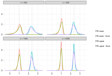
Figure 7: Empirical distribution of the lower and upper end of the PIR as well as the corresponding bootstrap distributions.

In order to investigate the coverage of bootstrap sensitivity intervals more closely, we consider the distribution of the estimated upper and lower end of the PIR as well as the corresponding bootstrap distributions. Figure 7 depicts the estimates of these distributions based on 1000 repitions of the experiment. For small sample sizes $n$, we notice that the bootstrap distribution is both biased and skewed. Both phenomena diminish as $n$ grows so that the bootstrap distribution approximates the target distribution more closely. This is in line with the observation that coverage moderately improves for larger sample sizes, especially for basic bootstrap.

S5.2 Linear Instrumental Variable Simulation

We generate 100 i.i.d. samples from the distribution $(\varepsilon_{U},\varepsilon_{Z},\varepsilon_{D},\varepsilon_{Y})^{T}\sim\mathcal{N}(0,\mathrm{Id})$ and compute the variables of the model as follows

$$U:=\varepsilon_{U},\quad Z:=\varepsilon_{Z},\quad D:=Z+U+\varepsilon_{D},\quad Y:=D+U+\varepsilon_{Y}.$$

This data-generating process fulfills the instrumental variable assumptions which renders $\beta=1$ point identified. Hence, a sensitivity interval where the IV-related sensitivity parameters are set to zero ought to be comparable with the confidence interval that is based on the asymptotic normality of the TSLS estimator. In order to use Algorithm 1, we slightly relax the IV assumptions requiring $R_{Z\sim U|X},R_{Y\sim Z|X,U,D}\!\in[-0.002,0.002]$ and further set $R_{D\sim U|X,Z}\in[-0.999,0.999]$ to bound it away from $-1$ and $1$.

We compute the empirical coverage and length of sensitivity intervals constructed via percentile, basic and BCa bootstrap, the heuristic sensitivity intervals and the oracle confidence intervals over 500 repitions of the experiment. Due to the high computational costs, we conduct this simulation study only for sample size $n=100$.

Table 4: Simulation results of the instrumental variable example.

Method	Coverage	Length
		Mean	Median
Percentile bootstrap	91.2%	0.327	0.300
Basic bootstrap	93.8%	0.260	0.235
BCa bootstrap	91.2%	0.329	0.300
Heuristic	98.6%	1.070	0.567
Oracle	93.0%	0.276	0.252

The results of this experiment are stated in Table 4. We notice that the bootstrap sensitivity intervals are on par with the oracle confidence interval, both in terms of coverage and length. By contrast, the heuristic sensitivity intervals exhibit very high coverage but their length is too long to be informative in practice. In this simulation study, 12 of the $500\cdot 500=250,000$ constructed bootstrap samples led to an empty constraint set.

S6 Derivation of Comparison Points for R-contour Plots

In Section 6.2.2, we introduce comparison points to provide context for the strength of the unmeasured confounder $U$ in relation to an observed covariate $\dot{X}_{j}$. To shorten the notation in the following, we introduce the abbreviation $W:=(\tilde{X},\dot{X}_{-j},Z)$. In the main text, we consider the case where $U$ explains $b$ times as much variance in $D$ and $Y$ as $\dot{X}_{j}$ does – conditional on $W$ or $(W,D)$. Here, we consider the more general case, where the multiplicative constant $b$ may be different for the relationship between $U\rightarrow D$ and $U\rightarrow Y$. We indicate this with a corresponding subscript.

First, we consider the sensitivity parameter $R_{D\sim U|X,Z}$. Due to (2), if $U$ explains $b_{D}$ times as much variance of $D$ as $\dot{X}_{j}$ – conditional on $W$ – and the respective correlations of $U$ and $\dot{X}_{j}$ with $D$ have the same sign, then

$$R_{D\sim U|X,Z}=\sqrt{b_{D}}\,\frac{R_{D\sim\dot{X}_{j}|W}}{\sqrt{1-R^{2}_{D\sim\dot{X}_{j}|W}}}=\sqrt{b_{D}}\,f_{D\sim\dot{X}_{j}|W}.$$ (S8)

In the following, we derive a similar formula for $R_{Y\sim U|X,Z,D}$ both for comparisons unconditional on $D$ and conditional on $D$. In either case, we make use of the following equation which follows from applying rule [vi] of the $R^{2}$-calculus with $Y\equiv Y$, $X\equiv\dot{X}_{j}$, $W\equiv D$ and $Z=W$:

$$R_{Y\sim D|W,\dot{X}_{j}}\stackrel{{\scriptstyle\text{[vi]}}}{{=}}\frac{1}{R_{D\sim\dot{X}_{j}|W}}\!\left[f_{Y\sim\dot{X}_{j}|W}\,\sqrt{1-R^{2}_{D\sim\dot{X}_{j}|W}}-f_{Y\sim\dot{X}_{j}|W,D}\,\sqrt{1-R^{2}_{Y\sim D|W,\dot{X}_{j}}}\right]\!.$$ (S9)

S6.1 Comparison unconditional on $D$

Assuming that $U$ explains $b_{Y}$ times as much variance in $Y$ as $\dot{X}_{j}$ does – conditional on $W$ – and that the respective correlations have the same sign, (2) implies

$$R_{Y\sim U|W,\dot{X}_{j}}=\sqrt{b_{Y}}\,\frac{R_{Y\sim\dot{X}_{j}|W}}{\sqrt{1-R^{2}_{Y\sim\dot{X}_{j}|W}}}=\sqrt{b_{Y}}f_{Y\sim\dot{X}_{j}|W}.$$

Inserting this relationship as well as (S8) into (2) yields

$$R_{Y\sim U|X,Z,D}=R_{Y\sim U|W,\dot{X}_{j},D}=\frac{\sqrt{b_{Y}}f_{Y\sim\dot{X}_{j}|W}-R_{Y\sim D|W,\dot{X}_{j}}\,\sqrt{b_{D}}f_{D\sim\dot{X}_{j}|W}}{\sqrt{1-R^{2}_{Y\sim D|W,\dot{X}_{j}}}\sqrt{1-b_{D}f_{D\sim\dot{X}_{j}|W}^{2}}}.$$

We reformulate this expression by invoking (S9), multiplying numerator and denominator with $\sqrt{1-R^{2}_{Y\sim\dot{X}_{j}|W}}$ and applying rule [iii] of the $R^{2}$-calculus

$$R_{Y\sim U|X,Z,D}=\frac{\left(\sqrt{b_{Y}}-\sqrt{b_{D}}\right)\,R_{Y\sim\dot{X}_{j}|W}+\sqrt{b_{D}}\,\sqrt{\frac{1-R^{2}_{Y\sim D+\dot{X}_{j}|W}}{1-R^{2}_{D\sim\dot{X}_{j}|W}}}\,f_{Y\sim\dot{X}_{j}|W,D}}{\sqrt{1-R^{2}_{Y\sim D+\dot{X}_{j}|W}}\sqrt{1-b_{D}f_{D\sim\dot{X}_{j}|W}^{2}}}.$$

Equation (19) follows from setting $b_{Y}=b_{D}=b$ and simplifying the resulting expression.

S6.2 Comparison conditional on $D$

Assuming that $U$ explains $b_{Y}$ times as much variance in $Y$ as $\dot{X}_{j}$ does – conditional on $W$ and $D$ – and that the respective correlations have the same sign implies

$$R_{Y\sim U|W,D}=\sqrt{b_{Y}}R_{Y\sim\dot{X}_{j}|W,D}.$$

Plugging this relationship as well as (S8) into (2) leads to

$$R_{Y\sim U|W,\dot{X}_{j}}=\frac{1}{\sqrt{1-R^{2}_{Y\sim\dot{X}_{j}|W}}}\bigg{[}R_{Y\sim D|W}\,\sqrt{b_{D}}\,R_{D\sim\dot{X}_{j}|W}\\ +\sqrt{b_{Y}}\,R_{Y\sim\dot{X}_{j}|W,D}\,\sqrt{1-R^{2}_{Y\sim D|W}}\sqrt{1-b_{D}R^{2}_{D\sim\dot{X}_{j}|W}}\bigg{]}.$$

To get a formula for $R_{Y\sim U|X,Z,D}$, we insert the equation above into (2), multiply numerator and denominator by $\sqrt{1-R^{2}_{Y\sim\dot{X}_{j}|W}}$, simplify the resulting expression via rule [iii] and obtain

$$R_{Y\sim U|X,Z,D}=-\frac{R_{Y\sim D|W,\dot{X}_{j}}\,\sqrt{b_{D}}f_{D\sim\dot{X}_{j}|W}\sqrt{1-R^{2}_{Y\sim\dot{X}_{j}|W}}}{\sqrt{1-R^{2}_{Y\sim D+\dot{X}_{j}|W}}\sqrt{1-b_{D}f_{D\sim\dot{X}_{j}|W}^{2}}}\\[6.45831pt] +\frac{R_{Y\sim D|W}\,\sqrt{b_{D}}\,R_{D\sim\dot{X}_{j}|W}+\sqrt{b_{Y}}\,R_{Y\sim\dot{X}_{j}|W,D}\,\sqrt{1-R^{2}_{Y\sim D|W}}\sqrt{1-b_{D}R^{2}_{D\sim\dot{X}_{j}|W}}}{\sqrt{1-R^{2}_{Y\sim D+\dot{X}_{j}|W}}\sqrt{1-b_{D}f_{D\sim\dot{X}_{j}|W}^{2}}}.$$

Invoking (S9) in the first equality below and applying rule [iv] with $Y\equiv Y$, $X\equiv\dot{X}_{j}$, $W\equiv D$ and $Z\equiv W$ in the second, we arrive at

$$R_{Y\sim U|X,Z,D} =\begin{multlined}\frac{\sqrt{b_{D}}(R_{Y\sim D|W}\,R_{D\sim\dot{X}_{j}|W}-R_{Y\sim\dot{X}_{j}|W})+\sqrt{b_{D}}\,\sqrt{\frac{1-R^{2}_{Y\sim D+\dot{X}_{j}|W}}{1-R^{2}_{D\sim X_{j}|W}}}\,f_{Y\sim\dot{X}_{j}|W,D}}{\sqrt{1-R^{2}_{Y\sim D+\dot{X}_{j}|W}}\sqrt{1-b_{D}f_{D\sim\dot{X}_{j}|W}^{2}}}\\[4.30554pt] +\frac{\sqrt{b_{Y}}\,R_{Y\sim\dot{X}_{j}|W,D}\,\sqrt{1-R^{2}_{Y\sim D|W}}\sqrt{1-b_{D}R^{2}_{D\sim\dot{X}_{j}|W}}}{\sqrt{1-R^{2}_{Y\sim D+\dot{X}_{j}|W}}\sqrt{1-b_{D}f_{D\sim\dot{X}_{j}|W}^{2}}}\end{multlined}\frac{\sqrt{b_{D}}(R_{Y\sim D|W}\,R_{D\sim\dot{X}_{j}|W}-R_{Y\sim\dot{X}_{j}|W})+\sqrt{b_{D}}\,\sqrt{\frac{1-R^{2}_{Y\sim D+\dot{X}_{j}|W}}{1-R^{2}_{D\sim X_{j}|W}}}\,f_{Y\sim\dot{X}_{j}|W,D}}{\sqrt{1-R^{2}_{Y\sim D+\dot{X}_{j}|W}}\sqrt{1-b_{D}f_{D\sim\dot{X}_{j}|W}^{2}}}\\[4.30554pt] +\frac{\sqrt{b_{Y}}\,R_{Y\sim\dot{X}_{j}|W,D}\,\sqrt{1-R^{2}_{Y\sim D|W}}\sqrt{1-b_{D}R^{2}_{D\sim\dot{X}_{j}|W}}}{\sqrt{1-R^{2}_{Y\sim D+\dot{X}_{j}|W}}\sqrt{1-b_{D}f_{D\sim\dot{X}_{j}|W}^{2}}}$$

$$=\begin{multlined}\frac{\left(\sqrt{b_{Y}}\sqrt{1-b_{D}R^{2}_{D\sim\dot{X}_{j}|W}}-\sqrt{b_{D}}\sqrt{1-R^{2}_{D\sim\dot{X}_{j}|W}}\right)R_{Y\sim\dot{X}_{j}|W,D}\,\sqrt{1-R^{2}_{Y\sim D|W}}}{\sqrt{1-R^{2}_{Y\sim D+\dot{X}_{j}|W}}\sqrt{1-b_{D}f_{D\sim\dot{X}_{j}|W}^{2}}}\\[4.30554pt] +\frac{\sqrt{b_{D}}\,\sqrt{\frac{1-R^{2}_{Y\sim D+\dot{X}_{j}|W}}{1-R^{2}_{D\sim X_{j}|W}}}\,f_{Y\sim\dot{X}_{j}|W,D}}{\sqrt{1-R^{2}_{Y\sim D+\dot{X}_{j}|W}}\sqrt{1-b_{D}f_{D\sim\dot{X}_{j}|W}^{2}}}.\end{multlined}\frac{\left(\sqrt{b_{Y}}\sqrt{1-b_{D}R^{2}_{D\sim\dot{X}_{j}|W}}-\sqrt{b_{D}}\sqrt{1-R^{2}_{D\sim\dot{X}_{j}|W}}\right)R_{Y\sim\dot{X}_{j}|W,D}\,\sqrt{1-R^{2}_{Y\sim D|W}}}{\sqrt{1-R^{2}_{Y\sim D+\dot{X}_{j}|W}}\sqrt{1-b_{D}f_{D\sim\dot{X}_{j}|W}^{2}}}\\[4.30554pt] +\frac{\sqrt{b_{D}}\,\sqrt{\frac{1-R^{2}_{Y\sim D+\dot{X}_{j}|W}}{1-R^{2}_{D\sim X_{j}|W}}}\,f_{Y\sim\dot{X}_{j}|W,D}}{\sqrt{1-R^{2}_{Y\sim D+\dot{X}_{j}|W}}\sqrt{1-b_{D}f_{D\sim\dot{X}_{j}|W}^{2}}}.$$

Equation (20) now follows from setting $b_{Y}=b_{D}=b$ and simplifying the resulting expression.

S7 Choice of Hyper-parameters

Table 5: Hyper-parameters for different plots and simulation examples.

	$N_{\text{grid}}$	$N_{\text{b-contour}}$	$N_{\text{boot}}$
Figure 2	200	-	3500
Figure 3	200	30	-
Figure 4	150	30	-
Figure 5	400	-	-
Figure 6	300	-	-
Table 3	200	-	1500
Table 4	100	-	500

In Table 5, we list the hyper-parameters of Algorithm 1 that were used for different data analyses. The mesh size of the grid is the same in every dimension, that is the numbers of points considered per dimension $N_{a}$, $N_{b}$, and $N_{g}$ are equal. We define $N_{\text{grid}}:=N_{a}=~{}N_{b}=~{}N_{g}$. The number of points per dimension for $b$-contour plots and the number of bootstrap samples are denoted by $N_{\text{b-contour}}$ and $N_{\text{boot}}$, respectively.

In the simulation study and data example in this work, we found that the PIR estimates change only marginally for values of $N_{\text{grid}}$ larger than 200. We recommend to consider at least 100 points per grid dimension, i.e. $N_{\text{grid}}=100$. The rough structure of the $b$-contours often becomes apparent for $N_{\text{b-contour}}$ as low as $10$. Due to the computational costs of the optimization problem, we choose a relatively low number of bootstrap samples. The simulation studies empirically confirm that percentile and BCa bootstrap sensitivity intervals achieve good coverage nonetheless.

References

- Altonji et al. (2005) Altonji, J. G., Elder, T. E. and Taber, C. R. (2005) An Evaluation of Instrumental Variable Strategies for Estimating the Effects of Catholic Schooling. Journal of Human Resources, XL, 791–821.
- Anderson (1958) Anderson, T. W. (1958) An introduction to multivariate statistical analysis. New York; London: Wiley Publications in Mathematical Statistics, 1st edn.
- Angrist and Pischke (2009) Angrist, J. D. and Pischke, J.-S. (2009) Mostly harmless econometrics: An empiricist’s companion. Princeton University Press.
- Aronow and Lee (2013) Aronow, P. M. and Lee, D. K. K. (2013) Interval estimation of population means under unknown but bounded probabilities of sample selection. Biometrika, 100, 235–240.
- Baba et al. (2004) Baba, K., Shibata, R. and Sibuya, M. (2004) Partial correlation and conditional correlation as measures of conditional independence. Australian & New Zealand Journal of Statistics, 46, 657–664.
- Balke and Pearl (1997) Balke, A. and Pearl, J. (1997) Bounds on Treatment Effects from Studies with Imperfect Compliance. Journal of the American Statistical Association, 92, 1171–1176.
- Blackwell (2014) Blackwell, M. (2014) A Selection Bias Approach to Sensitivity Analysis for Causal Effects. Political Analysis, 22, 169–182.
- Card (1993) Card, D. (1993) Using Geographic Variation in College Proximity to Estimate the Return to Schooling. Tech. Rep. w4483, National Bureau of Economic Research, Cambridge, MA.
- Chernozhukov et al. (2022) Chernozhukov, V., Cinelli, C., Newey, W., Sharma, A. and Syrgkanis, V. (2022) Long Story Short: Omitted Variable Bias in Causal Machine Learning. Tech. Rep. w30302, National Bureau of Economic Research, Cambridge, MA.
- Chernozhukov et al. (2007) Chernozhukov, V., Hong, H. and Tamer, E. (2007) Estimation and Confidence Regions for Parameter Sets in Econometric Models. Econometrica, 75, 1243–1284.
- Cinelli and Hazlett (2020) Cinelli, C. and Hazlett, C. (2020) Making sense of sensitivity: extending omitted variable bias. Journal of the Royal Statistical Society: Series B (Statistical Methodology), 82, 39–67.
- Cochran (1938) Cochran, W. G. (1938) The Omission or Addition of an Independent Variate in Multiple Linear Regression. Supplement to the Journal of the Royal Statistical Society, 5, 171.
- Cohen (1977) Cohen, J. (1977) Statistical power analysis for the behavioral sciences. New York: Academic Press, rev. edn.
- Colnet et al. (2022) Colnet, B., Josse, J., Varoquaux, G. and Scornet, E. (2022) Causal effect on a target population: A sensitivity analysis to handle missing covariates. Journal of Causal Inference, 10, 372–414.
- Cornfield et al. (1959) Cornfield, J., Haenszel, W., Hammond, E. C., Lilienfeld, A. M., Shimkin, M. B. and Wynder, E. L. (1959) Smoking and lung cancer: recent evidence and a discussion of some questions. Journal of the National Cancer institute, 22, 173–203.
- Cox (2007) Cox, D. R. (2007) On a generalization of a result of W. G. Cochran. Biometrika, 94, 755–759.
- Davidson and MacKinnon (1993) Davidson, R. and MacKinnon, J. G. (1993) Estimation and inference in econometrics. New York: Oxford University Press.
- Davison and Hinkley (1997) Davison, A. C. and Hinkley, D. V. (1997) Bootstrap Methods and their Application. Cambridge University Press, 1st edn.
- Dawid (1979) Dawid, A. P. (1979) Conditional independence in statistical theory. Journal of the Royal Statistical Society: Series B (Statistical Methodology), 41, 1–15.
- Ding and VanderWeele (2016) Ding, P. and VanderWeele, T. J. (2016) Sensitivity Analysis Without Assumptions. Epidemiology, 27, 368–377.
- Dorn and Guo (2022) Dorn, J. and Guo, K. (2022) Sharp Sensitivity Analysis for Inverse Propensity Weighting via Quantile Balancing. Journal of the American Statistical Association, 1–13.
- Efron and Tibshirani (1994) Efron, B. and Tibshirani, R. (1994) An Introduction to the Bootstrap. Chapman and Hall/CRC.
- Frank (2000) Frank, K. A. (2000) Impact of a Confounding Variable on a Regression Coefficient. Sociological Methods & Research, 29, 147–194.
- Guo et al. (2022) Guo, W., Yin, M., Wang, Y. and Jordan, M. (2022) Partial Identification with Noisy Covariates: A Robust Optimization Approach. In Proceedings of the First Conference on Causal Learning and Reasoning, 318–335. PMLR.
- Halmos (2000) Halmos, P. R. (2000) Introduction to Hilbert space and the theory of spectral multiplicity. Providence, R.I.: AMS Chelsea, 2nd edn.
- Hernan and Robins (1999) Hernan, M. A. and Robins, J. M. (1999) Letter to the editor of biometrics. Biometrics, 55, 1316–1317.
- Hosman et al. (2010) Hosman, C. A., Hansen, B. B. and Holland, P. W. (2010) The sensitivity of linear regression coefficients’ confidence limits to the omission of a confounder. The Annals of Applied Statistics, 4.
- Hu et al. (2021) Hu, Y., Wu, Y., Zhang, L. and Wu, X. (2021) A Generative Adversarial Framework for Bounding Confounded Causal Effects. Proceedings of the AAAI Conference on Artificial Intelligence, 35, 12104–12112.
- Imbens (2003) Imbens, G. W. (2003) Sensitivity to exogeneity assumptions in program evaluation. American Economic Review, 93, 126–132.
- Imbens and Manski (2004) Imbens, G. W. and Manski, C. F. (2004) Confidence Intervals for Partially Identified Parameters. Econometrica, 72, 1845–1857.
- Kaido et al. (2019) Kaido, H., Molinari, F. and Stoye, J. (2019) Confidence intervals for projections of partially identified parameters. Econometrica, 87, 1397–1432.
- Lin et al. (1998) Lin, D. Y., Psaty, B. M. and Kronmal, R. A. (1998) Assessing the Sensitivity of Regression Results to Unmeasured Confounders in Observational Studies. Biometrics, 54, 948–963.
- Manski (1990) Manski, C. F. (1990) Nonparametric Bounds on Treatment Effects. The American Economic Review, 80, 319–323.
- Manski (2003) — (2003) Partial Identification of Probability Distributions. Springer Series in Statistics. New York: Springer.
- Miratrix et al. (2018) Miratrix, L. W., Wager, S. and Zubizarreta, J. R. (2018) Shape-constrained partial identification of a population mean under unknown probabilities of sample selection. Biometrika, 105, 103–114.
- Molinari (2020) Molinari, F. (2020) Chapter 5 - Microeconometrics with Partial Identification. In Handbook of Econometrics, vol. 7, 355–486. Elsevier.
- Nagar (1959) Nagar, A. L. (1959) The Bias and Moment Matrix of the General k-Class Estimators of the Parameters in Simultaneous Equations. Econometrica, 27, 575–595.
- Oster (2019) Oster, E. (2019) Unobservable Selection and Coefficient Stability: Theory and Evidence. Journal of Business & Economic Statistics, 37, 187–204.
- Padh et al. (2023) Padh, K., Zeitler, J., Watson, D., Kusner, M., Silva, R. and Kilbertus, N. (2023) Stochastic causal programming for bounding treatment effects. In Proceedings of the Second Conference on Causal Learning and Reasoning, vol. 213 of Proceedings of Machine Learning Research, 142–176. PMLR.
- PCORI Methodology Committee (2021) PCORI Methodology Committee (2021) The PCORI Methodology Report. https://www.pcori.org/sites/default/files/PCORI-Methodology-Report.pdf.
- Pearl (2009) Pearl, J. (2009) Causality: Models, Reasoning, and Inference. Cambridge University Press, 2 edn.
- Richardson et al. (2014) Richardson, A., Hudgens, M. G., Gilbert, P. B. and Fine, J. P. (2014) Nonparametric Bounds and Sensitivity Analysis of Treatment Effects. Statistical Science, 29, 596–618.
- Rosenbaum (1987) Rosenbaum, P. R. (1987) Sensitivity analysis for certain permutation inferences in matched observational studies. Biometrika, 74, 13–26.
- Rosenbaum (2002) — (2002) Observational Studies. Springer Series in Statistics. New York: Springer.
- Rosenbaum and Rubin (1983) Rosenbaum, P. R. and Rubin, D. B. (1983) Assessing Sensitivity to an Unobserved Binary Covariate in an Observational Study with Binary Outcome. Journal of the Royal Statistical Society: Series B (Statistical Methodology), 45, 212–218.
- Rothenhäusler et al. (2021) Rothenhäusler, D., Meinshausen, N., Bühlmann, P. and Peters, J. (2021) Anchor regression: Heterogeneous data meet causality. Journal of the Royal Statistical Society: Series B (Statistical Methodology), 83, 215–246.
- Rubinstein and Shapiro (1993) Rubinstein, R. Y. and Shapiro, A. (1993) Discrete event systems. Sensitivity analysis and stochastic optimization by the score function method. Chichester: John Wiley & Sons.
- Scharfstein et al. (1999) Scharfstein, D. O., Rotnitzky, A. and Robins, J. M. (1999) Adjusting for Nonignorable Drop-Out Using Semiparametric Nonresponse Models. Journal of the American Statistical Association, 94, 1096–1120.
- Shapiro (1991) Shapiro, A. (1991) Asymptotic analysis of stochastic programs. Annals of Operations Research, 30, 169–186.
- Shapiro et al. (2009) Shapiro, A., Dentcheva, D. and Ruszczyński, A. (2009) Lectures on Stochastic Programming: Modeling and Theory. Society for Industrial and Applied Mathematics.
- Small (2007) Small, D. S. (2007) Sensitivity Analysis for Instrumental Variables Regression With Overidentifying Restrictions. Journal of the American Statistical Association, 102, 1049–1058.
- de Souza et al. (2016) de Souza, R. J., Eisen, R. B., Perera, S., Bantoto, B., Bawor, M., Dennis, B. B., Samaan, Z. and Thabane, L. (2016) Best (but oft-forgotten) practices: sensitivity analyses in randomized controlled trials. The American Journal of Clinical Nutrition, 103, 5–17.
- Spirtes et al. (2000) Spirtes, P., Glymour, C. N., Scheines, R. and Heckerman, D. (2000) Causation, Prediction, and Search. MIT Press.
- Stoye (2009) Stoye, J. (2009) More on Confidence Intervals for Partially Identified Parameters. Econometrica, 77, 1299–1315.
- Thabane et al. (2013) Thabane, L., Mbuagbaw, L., Zhang, S., Samaan, Z., Marcucci, M., Ye, C., Thabane, M., Giangregorio, L., Dennis, B., Kosa, D., Debono, V. B., Dillenburg, R., Fruci, V., Bawor, M., Lee, J., Wells, G. and Goldsmith, C. H. (2013) A tutorial on sensitivity analyses in clinical trials: the what, why, when and how. BMC Medical Research Methodology, 13, 92.
- Theil (1958) Theil, H. (1958) Economist Forecasts and Policy. North-Holland Publishing Company, Amsterdam-London.
- Tudball et al. (2022) Tudball, M. J., Hughes, R. A., Tilling, K., Bowden, J. and Zhao, Q. (2022) Sample-constrained partial identification with application to selection bias. Biometrika, 110, 485–498.
- Vandenbroucke et al. (2007) Vandenbroucke, J. P., von Elm, E., Altman, D. G., Gøtzsche, P. C., Mulrow, C. D., Pocock, S. J., Poole, C., Schlesselman, J. J. and Egger, M. (2007) Strengthening the Reporting of Observational Studies in Epidemiology (STROBE): Explanation and Elaboration. PLoS Medicine, 4, e297.
- VanderWeele and Arah (2011) VanderWeele, T. J. and Arah, O. A. (2011) Bias Formulas for Sensitivity Analysis of Unmeasured Confounding for General Outcomes, Treatments, and Confounders. Epidemiology, 22, 42–52.
- Vansteelandt et al. (2006) Vansteelandt, S., Goetghebeur, E., Kenward, M. G. and Molenberghs, G. (2006) Ignorance and Uncertainty Regions as Inferential Tools in a Sensitivity Analysis. Statistica Sinica, 16, 953–979.
- Veitch and Zaveri (2020) Veitch, V. and Zaveri, A. (2020) Sense and Sensitivity Analysis: Simple Post-Hoc Analysis of Bias Due to Unobserved Confounding. In Advances in Neural Information Processing Systems, vol. 33, 10999–11009. Curran Associates, Inc.
- Wooldridge (2010) Wooldridge, J. M. (2010) Econometric analysis of cross section and panel data. Cambridge, Mass: MIT Press, 2nd edn.
- Yadlowsky et al. (2022) Yadlowsky, S., Namkoong, H., Basu, S., Duchi, J. and Tian, L. (2022) Bounds on the conditional and average treatment effect with unobserved confounding factors. The Annals of Statistics, 50, 2587–2615.
- Zhang and Ding (2022) Zhang, M. and Ding, P. (2022) Interpretable sensitivity analysis for the Baron-Kenny approach to mediation with unmeasured confounding. arXiv:2205.08030.
- Zhao et al. (2019) Zhao, Q., Small, D. S. and Bhattacharya, B. B. (2019) Sensitivity analysis for inverse probability weighting estimators via the percentile bootstrap. Journal of the Royal Statistical Society: Series B (Statistical Methodology), 81, 735–761.
- Zheng et al. (2021) Zheng, J., D’Amour, A. and Franks, A. (2021) Copula-based Sensitivity Analysis for Multi-Treatment Causal Inference with Unobserved Confounding. arXiv: 2102.09412.
- Zheng et al. (2023) Zheng, J., Wu, J., D’Amour, A. and Franks, A. (2023) Sensitivity to Unobserved Confounding in Studies with Factor-Structured Outcomes. Journal of the American Statistical Association, 0, 1–12.