CEERS Key Paper IV: Galaxies at $\mathbf{4<z<9}$ are Bluer than They Appear —
Characterizing Galaxy Stellar Populations from Rest-Frame $\mathrm{\sim}$1 micron Imaging

Abstract

We present results from the Cosmic Evolution Early Release Survey (CEERS) on the stellar-population parameters for 28 galaxies with redshifts $4<z<9$ using imaging data from the James Webb Space Telescope (JWST) Mid-Infrared Instrument (MIRI) combined with data from the Hubble Space Telescope and the Spitzer Space Telescope. The JWST/MIRI 5.6 and 7.7 µm data extend the coverage of the rest-frame spectral-energy distribution (SED) to nearly 1 micron for galaxies in this redshift range. By modeling the galaxies’ SEDs the MIRI data show that the galaxies have, on average, rest-frame UV (1600 Å) – $I$-band colors 0.4 mag bluer than derived when using photometry that lacks MIRI. Therefore, the galaxies have lower stellar-mass–to–light ratios. The MIRI data reduce the stellar masses by $\langle\Delta\log M_{\ast}\rangle=0.25$ dex at $4<z<6$ and 0.37 dex at $6<z<9$ .This also reduces the star-formation rates (SFRs) by $\langle\Delta\log\mathrm{SFR}\rangle=0.14$ dex at $4<z<6$ and 0.27 dex at $6<z<9$. The MIRI data also improve constraints on the allowable stellar mass formed in early star-formation. We model this using a star-formation history that includes both a “burst’ at $z_{f}=100$ and a slowly varying (“delayed-$\tau$”) model. The MIRI data reduce the allowable stellar mass by 0.6 dex at $4<z<6$ and by $\approx$1 dex at $6<z<9$. Applying these results globally, this reduces the cosmic stellar-mass density by an order of magnitude in the early universe ($z\approx 9$). Therefore, observations of rest-frame $\mathrel{\hbox{\hbox to0.0pt{\hbox{\lower 4.0pt\hbox{$\sim$}}\hss}\hbox{$>$}}}$1 µm are paramount for constraining the stellar–mass build-up in galaxies at very high-redshifts.

1 Introduction

There is growing evidence that galaxies must have started forming stars very quickly following the Big Bang. Theory predicts the first stars should form at $z\mathrel{\hbox{\hbox to0.0pt{\hbox{\lower 4.0pt\hbox{$\sim$}}\hss}\hbox{$>$}}}20$ (e.g., Barkana & Loeb 2001; Miralda-Escudé 2003; Yoshida et al. 2003; Wise et al. 2012; Visbal et al. 2020). The ionization from these sources is needed to explain observations that the hydrogen-neutral fraction of the intergalactic medium (IGM) was 50% by $z\sim 8$ (Planck Collaboration et al. 2020), . Indeed, early observations from JWST have already identified candidates for galaxies at $z\mathrel{\hbox{\hbox to0.0pt{\hbox{\lower 4.0pt\hbox{$\sim$}}\hss}\hbox{$>$}}}15$ (Curtis-Lake et al. 2022; Donnan et al. 2022; Finkelstein et al. 2022a; Robertson et al. 2022). Spectroscopy from JWST of galaxies at $z\sim 8-9$ shows emission lines from heavy elements that appear to require metallicities of $\approx 5-10\%~{}Z_{\odot}$ (Arellano-Córdova et al. 2022; Fujimoto et al. 2022; Heintz et al. 2022; Langeroodi et al. 2022; Matthee et al. 2022; Schaerer et al. 2022; Trump et al. 2022; Curti et al. 2023; Katz et al. 2023), implying these galaxies have experienced at least one (and probably multiple) generation(s) of previous stars. This is consistent with earlier detections of metal lines in $z>6$ galaxies from ground-based telescopes (e.g., Stark et al. 2017; Hutchison et al. 2019). All of these results point to the fact that star formation began early and those early generations of stars enriched the universe with heavy elements.

It is then important to consider how we may constrain the history of star-formation in these early galaxies. The number of stars, and therefore the stellar mass, in galaxies appears to rise rapidly. The (co-moving) stellar mass density in galaxies at $z\sim 5-6$ is already 1% of the present value (e.g., Madau & Dickinson 2014; Finkelstein 2016). Obviously these stars must form at earlier times, and because the age of the Universe is only $\approx 1$ Gyr at these redshifts, the time to form these stars is relatively short.

Even early JWST observations find some evidence for massive galaxies at $z>7$ (Labbé et al. 2022) with some candidate objects having masses, $\log M_{\ast}/M_{\odot}>11$ , as large as the stellar mass of the Milky Way today (e.g., Papovich et al. 2015). Such objects would be in tension with galaxy formation models (Boylan-Kolchin 2022) where there are not sufficient numbers of massive dark-mater halos to support these objects, even if all the baryons in the halos are in the form of stellar mass. However, the uncertainty in these measurements is in the assumed star-formation histories, the contributions of emission lines to the photometric measurements from broad-band data (e.g., Endsley et al. 2022; Pérez-González et al. 2022; Steinhardt et al. 2022), and the effects of young stellar populations “outshining” older stellar populations in the integrated emission of galaxies (e.g., Giménez-Arteaga et al. 2022). Clearly there are unknown systematics in the assumptions of the data analysis, or missing physics in our theoretical understanding of stellar populations and galaxy formation, or some combination of all of these things. It is therefore crucial to understand constraints on the stellar masses (which are the integral of the star-formation histories) as much as possible.

Motivated by these issues, in this Paper we use new data from JWST to better constrain the stellar masses, star-formation rates (SFRs), and star-formation histories of galaxies during the first one and a half billion years after the Big Bang ($z>4$). One of the problems with initial studies from JWST is that they currently rely entirely on observations from JWST’s Near-IR Camera (NIRcam), which only probes to wavelengths $\mathrel{\hbox{\hbox to0.0pt{\hbox{\lower 4.0pt\hbox{$\sim$}}\hss}\hbox{$<$}}}$5 µm, or about 6000 Å rest-frame for $z=6-7$ galaxies. This complicates the ability to disentangle massive galaxies with older stellar populations from younger, dusty galaxies or galaxies with emission lines with extreme equivalent widths (see discussion in Antwi-Danso et al. 2022, and recent work by Giménez-Arteaga et al. 2022 who find evidence for older stellar populations mixed with recent bursts in spatially resolved studies using JWST/NIRCam data). To better constrain the SEDs of these galaxies requires observations at longer wavelengths. This is where JWST/MIRI is important as it has the sensitivity to detect $z\approx 10$ galaxies at rest-frame 1 µm (see Bisigello et al. 2017). Previous work on this subject has been limited to data from the Spitzer Space Telescope, which is primarily sensitive to the emission of distant galaxies at 3.6 to 8.0 µm. JWST offers immense gains to Spitzer: JWST has a collecting area that is 45 times larger than that of Spitzer, and the larger aperture provides image quality (i.e., angular resolution) that is improved by a factor of order 10 (Rigby et al. 2022). These gains are especially manifest at longer wavelengths, and make JWST 5.6 and 7.7 µm data vastly more sensitive than Spitzer.

The outline for the Paper is as follows. In Section 2 we discuss the CEERS dataset and the ancillary datasets used in this study. We also discuss the processes to create (and validate) the flux densities of galaxies in the CEERS JWST/MIRI data at 5.6 and 7.7 µm. In Section 2.2 we discuss the sample of $4<z<9$ galaxies used in this study, and we present the MIRI data for these objects. In Section 3 we discuss the analysis methods to derive constraints on the galaxy stellar populations. In Section 4 we discuss the resulting improvements that including the MIRI data provide on constraints on the galaxies stellar populations (specifically their stellar–masses and SFRs) derived from fitting stellar population models to the observed photometry. In Section 4.4 we discuss constraints on the range of allowed stellar masses in these high redshift galaxies by allowing for an early (“maximally old”) burst of stars at $z=100$, and we show that adding the MIRI data improves the limit on this hypothetical population of $z=100$ stars by a factor of 6 to 10 for galaxies at $4<z<9$. In Section 5 we discuss the implications these constraints have for our understanding of galaxy colors, stellar populations at these high redshifts, and the evolution of the galaxy stellar mass density, in particular during the epoch of reionization, and what this could mean for future studies of galaxies at higher redshifts (from JWST). In Section 6 we present our conclusions and prospects for future studies.

Throughout we use a flat cosmology with $\Omega_{m,0}=0.315$, $H_{0}=67.4$ km s^-1 Mpc^-1 (Planck Collaboration et al. 2020). All magnitudes reported here are on the Absolute Bolometric (AB) system (Oke & Gunn 1983). Throughout we use the Chabrier (2003) initial mass function (IMF) for all stellar masses and SFRs. We denote magnitudes measured in the MIRI F560W and F770W bands as $[5.6]$ and $[7.7]$, respectively. Similarly, we denote magnitudes measured in IRAC Channel 1 (3.6 µm), Channel 2 (4.5 µm), Channel 3 (5.8 µm), and Channel 4 (8.0 µm) as $[3.6]$, $[4.5]$, $[5.8]$, and $[8.0]$, respectively.

2 Data and Sample

2.1 MIRI Catalog

We use the data release DR0.5 images produced by the CEERS team for the MIRI 3 and MIRI 6 fields (see Finkelstein et al. 2022a). These data were acquired in 2022 June 21 and 22. The properties of the data and the data reduction are discussed elsewhere (Yang et al. 2023, in prep), but we provide a summary here. The data were processed using the JWST Calibration Pipeline (v1.7.2) using the default parameters for stage 1 and 2. We then removed the backgrounds with a custom routine that combines images taken in the same bandpass but from different fields and/or dither positions, rejecting pixels in each image that contain galaxies, in order to create a “super-background” image. We then removed this background from each image and applied an astrometric correction to each image prior to processing them with stage 3 of the pipeline. This produced the final science images (extension i2d), rms images (extension rms, which account for Poisson, readout, and correlated pixel noise; see Yang et al. 2023, in prep), and weight maps (wht) for each field with a pixel scale of 0.09″, registered astrometrically to the existing HST/CANDELS v1.9 WFC3 and ACS images (see Koekemoer et al. 2011; Bagley et al. 20222). Our tests find that the MIRI images achieve limiting $5\sigma$ depths in the MIRI images of 26.5 and 27.1 AB mag measured in 0.45″-diameter apertures.

For the purpose of this study we are interested in sources detected in the MIRI data, so we create a catalog of sources derived from these images. Prior to object detection we convolved the 5.6 µm image to match the image quality of the 7.7 µm image. For this step, we constructed an “effective” point source function (ePSF) for each image by identifying unblended stars using the photutils (v1.5.0) detection task, and modeling them with the photutils psf task. This produced model ePSFs with measured full-width at half maxima (FWHM) of $0.24\arcsec$ and $0.28\arcsec$, for the F560W and F770W images, respectively. This is consistent with the expected image quality, but takes into account the exact dithering and reduction steps for the CEERS MIRI data. We then used PyPHER (Boucaud et al. 2016b) to construct a convolution kernel to match the image quality of the model ePSFs. We applied these kernels to each F560W image, creating a “PSF-matched” image. Our tests on point sources in the PSF-matched F560W and F770W images show that we measure the same fraction of light to better than 2% in fixed circular apertures of radii larger than $0{\farcs}35$.

We then created a detection image constructed from the sum of the MIRI F560W and F770W science images (using the extension sci) weighted by the appropriate weight image (using the extension wht). We also created a detection weight-map as the sum of the weights for these images. We then created F560W and F770W catalogs using Source Extractor (SE, version 2.19.5; Bertin & Arnouts 1996) in “dual-image” mode using the detection image and its weight map for object detection, where we measured photometry in the PSF-matched F560W and F770W image. We used the parameters in Table 1. We then measured fluxes and magnitudes using circular apertures of 0.9″ diameter, and we scaled these to a total aperture (MAG_AUTO) measured for each source in the detection image. Uncertainties for each object are measured from the rms image in the same apertures, and scaled to a total magnitude in the same way. .

Table 1: CEERS MIRI F560W and F770W SExtractor Parameter Settings

SExtractor Parameter	Value
(1)	(2)
DETECT_MINAREA	10 pixels
DETECT_THRESH	1.3
ANALYSIS_THRESH	1.3
FILTER_NAME	gauss_2.5_5x5
WEIGHT_TYPE	MAP_WEIGHT,MAP_RMS
DEBLEND_NTHRESH	32
DEBLEND_MINCONT	0.005
MAG_ZEROPOINT	25.701
PIXEL_SCALE	0.09 arcsec
BACK_TYPE	AUTO
BACK_FILTERSIZE	5 pixels
BACK_SIZE	32 pixels
BACKPHOTO_THICK	8
BACKPHOTO_TYPE	LOCAL
SEEING_FWHM	0.3 arcsec

Note. — SE was run using the weighted sum of the PSF-matched F560W and F770W images for detection, and using the images separately for photometry. All other SE parameters are set to the program defaults (for SExtractor v.2.19.5).

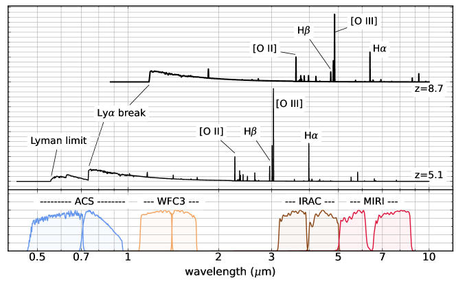
Figure 1: Illustration of galaxy spectra (in relative units of erg s^-1 cm^-2 Å^-1) compared to the broad-band data for the observations in this work. The bottom panel shows the relative transmission functions for the HST/ACS and WFC3 filters (ACS F606W, F814 and WFC3 F125W, F160W), Spitzer/IRAC 3.6 µm (Ch1) and 4.5 µm (Ch2), and JWST/MIRI F560W and F770W. The top panel shows model spectra of star-forming galaxies at $z=5.1$ and $z=8.7$, which match two galaxies with spectroscopic redshifts in this sample. Key emission lines and features are labeled. The MIRI data probe the shape of the galaxy spectral energy distributions to 8000 Å rest-frame, even for galaxies with $z=9$.

We compared the MIRI flux densities for sources with F560W and F770W detections against those for bright objects from existing IRAC 5.8 and 8.0 µm catalogs (Stefanon et al. 2017). For bright objects ($[5.8]$ or $[8.0]\leq 22$ AB mag) in the IRAC data, we measure small offsets of $\Delta m=\hbox{$[5.8]$}-\hbox{$[5.6]$}=0.16$ mag between the IRAC 5.8 and MIRI 5.6 data, and $\Delta m=\hbox{$[8.0]$}-\hbox{$[7.7]$}=0.07$ mag between the IRAC 8.0 and MIRI 7.7 data (i.e., the MIRI flux densities are slightly brighter). Most of these offsets can be explained by differences in the shape of the MIRI and IRAC passbands and because of differences in the angular resolution of the instruments (MIRI has a PSF FWHM smaller by a factor of more than seven). These tests are discussed more fully in Yang et al. (2023, in prep), but this gives us confidence that the MIRI data are calibrated to better than $\simeq 0.1-0.2$ mag.

Figure 2: Montage of images of a subset of the galaxies used in this study ordered by increasing redshift. Each row shows images for one galaxy (labeled by galaxy ID and redshift). The images are (left to right), ACS F606W, F814W, WFC3 F125, F160W, IRAC Ch1 (3.6 µm) and Ch2 (4.5 µm), and MIRI F560W and F770W. The images above include the three galaxies with spectroscopic redshifts (ID 37653, 19180, and 6811). The images are $6\arcsec\times 6\arcsec$ centered on the galaxy in each bandpass, as labeled along the top row. The complete figure set (28 images) is available online.

Fig. Set2. Montage of ACS F606W, F814W, WFC3 F125W, F140W, F160W, IRAC 3.6 and 4.5 µm, and MIRI 5.6 and 7.7 µm images for all galaxies in the sample (28 figures).

2.2 Galaxy Sample

For this study we use galaxies identified in the CEERS/MIRI first epoch fields with photometric redshifts $4.3<z<10$ from Finkelstein et al. (2022b). The lower redshift bound is selected to ensure the HST photometric data probe the redshifted Lyman-break. The upper redshift limit includes the highest redshift galaxies detectable by HST/WFC3 data (Bouwens et al. 2019; Finkelstein et al. 2022b). This is illustrated in Figure 1 which shows that for galaxies around $z\sim 5$ and $z\sim 9$, the HST/ACS and WFC3 data constrain this break. This improves the quality of the sample, as compared to, for example, using galaxies at $z\approx 3$ where the Lyman–break shifts blueward of the HST/ACS F606W band.

As mentioned above, the parent sample for our study is the catalog from Finkelstein et al. (2022b), which uses the existing HST/ACS, WFC3 and Spitzer/IRAC 3.6 and 4.5 µm data to select photometric samples of galaxies at these high redshifts. The data include both the imaging from the original CANDELS survey (HST/ACS F606W, F814W, WFC3 F125W, F160W) and additional imaging from WFC3 F140W (see Footnote 2). Finkelstein et al. (2022b) then use these data to measure photometric redshifts and redshift probably distribution functions, $P(z)$ for each object.

We matched objects from the catalog from Finkelstein et al. (2022b) with objects in our MIRI catalogs that are detected with S/N $>$ 3 in either the MIRI 5.6 or 7.7 µm data (Section 2.1) using a matching radius of 0.5″. This sample includes 29 objects, though one object was later identified as a foreground star and removed. Table 5 lists the observed properties of the 28 galaxies in the sample, their ID numbers from Finkelstein et al. (2022b), their HST/F160W flux densities the MIRI 5.6 and 7.7 µm flux densities. The table includes the photometric redshifts derived by Finkelstein et al. including the 16th and 84th-percentile range from the $P(z)$ used for object selection. The Table also includes the amount of the integrated $P(z)$ contained between $\Delta z=\pm 0.5$ of the stated redshift, for example,

$$\mathcal{P}(z=z_{c})=\int_{z_{c}-0.5}^{z_{c}+0.5}\ P(z^{\prime})\ dz^{\prime}$$ (1)

in bins with central redshifts of $z_{c}$ = 4, 5, 6, 7, 8, and 9 (see Finkelstein et al. 2022b). These integrated probabilities indicate a likelihood that a given galaxy is within the redshift bin to which it is assigned. For our analysis we rederive the photometric redshifts below (from SED modeling that includes the new 5.6 and 7.7 µm MIRI data) but include this here as we use the $P(z)$ in Table 5 as a prior likelihood on the SED fitting (discussed in Section 3 below).

Three of the galaxies in our sample have spectroscopic redshifts. This includes a previously known galaxy (ID 6811 in our catalog) with $z=8.683$ from Zitrin et al. (2015), and two new redshifts obtained by the CEERS and WERLS collaborations from observations with Keck/DEIMOS and Keck/LRIS. The latter two sources are ID 37653 with $z=4.899$ measured by (Stawinski et al. 2023a, in preparation) and ID 19180 with $z=5.077$ (Stawinski et al. 2023b, in preparation). In all of these cases the spectroscopic redshifts are consistent with the photometric redshifts in Table 5, and we fix the redshift to the value of the spectroscopic redshift in our analysis of the spectral energy distributions below.

Figure 2 shows the HST/ACS, HST/WFC3, Spitzer/IRAC, and JWST/MIRI imaging for all the objects in our sample, with the objects ordered by increasing redshift (the full Figure Set of all 28 objects is available online). In all cases the galaxies show prominent “Lyman–breaks” at the location of the redshifted Lyman-limit and/or Lyman-$\alpha$. In some cases, the flux density appears to be much brighter in a given passband compared to the adjacent band (for example, galaxy ID=12514 at $z=7.6$ shows evidence of enhanced emission at MIRI 5.6 µm, indicative of strong redshifted H$\alpha$). Figure 1 illustrates how the bandpasses are sensitive to different features in the SED of galaxies (using $z=5.1$ and $z=8.7$ as examples as these are similar to two of the objects with spectroscopic redshifts in our sample). We will return to these cases below when we explore constraints on the galaxy stellar populations by modeling their SEDs (Section 3).

The $4<z<9$ galaxies in our sample have MIRI $\hbox{$[5.6]$}-\hbox{$[7.7]$}$ colors largely consistent with expectations: most objects have relatively flat ($\hbox{$[5.6]$}-\hbox{$[7.7]$}\approx 0$ mag) or blue colors ($\hbox{$[5.6]$}-\hbox{$[7.7]$}\mathrel{\hbox{\hbox to0.0pt{\hbox{\lower 4.0pt\hbox{$\sim$}}\hss}\hbox{$<$}}}0$ mag). This implies that in most cases the MIRI data sample the continuum of galaxies. In some cases the MIRI colors suggest very blue colors, $\hbox{$[5.6]$}-\hbox{$[7.7]$}\mathrel{\hbox{\hbox to0.0pt{\hbox{\lower 4.0pt\hbox{$\sim$}}\hss}\hbox{$<$}}}-0.5$ to $-1$ mag. This could indicate the presence of an emission line in the F560W band that boosts the brightness in this band. We will explore evidence for this interpretation below.

3 Spectral Energy Distribution Modelling

We model the spectral energy distributions (SEDs) of the galaxies in our sample using stellar population synthesis models. Our goal is to test how the inferred properties of the stellar populations in the high-redshift galaxies change by including the JWST/MIRI 5.6 and 7.7 µm data, in particular the stellar masses and the SFRs. Previous work before the launch of JWST showed that MIRI data are able to recover these quantities accurately (Bisigello et al. 2017), and here we test how they improve the constraints on the stellar population parameters. This is critical for galaxies at higher redshifts, $z\mathrel{\hbox{\hbox to0.0pt{\hbox{\lower 4.0pt\hbox{$\sim$}}\hss}\hbox{$>$}}}4$, where the rest-frame optical features shift to longer wavelengths (rest-frame 4000 Å corresponds to $>$2 µm), which probes light from longer-lived stars.

Perhaps more problematic are the effects of nebular emission lines, which can litter the optical portion of the SED (see Figure 1). There are observations that $z>2$ galaxies have a higher incidence of “extreme” emission lines with rest-frame EWs up to $\approx$1000 Å (e.g., van der Wel et al. 2011; Tang et al. 2019; Tran et al. 2020; Boyett et al. 2022; Matthee et al. 2022; Pérez-González et al. 2022; Sun et al. 2022), consistent with inferences made from the $>$3 µm colors of $z>6$ galaxies (Smit et al. 2015; Roberts-Borsani et al. 2016; Castellano et al. 2017; Hutchison et al. 2019; Endsley et al. 2021). As the EW scales with redshift as $(1+z)$ this implies these lines have a stronger impact for high-redshift galaxies for bandpasses of fixed wavelength width (e.g. Papovich et al. 2001; Burgarella et al. 2022).

Table 2: Parameter Settings for BAGPIPES

Model	Parameter	Prior	Limits
Star-Formation History (1): Delayed-$\tau$, $\Psi\propto(t/\tau)\exp(-t/\tau)$	$e$-folding timescale, $\tau$ / Gyr	Uniform	(0.01, 10)
	age, $t$ / Gyr	Uniform	(0.01,15)
	stellar mass, $\log(M_{\ast}/M_{\odot})$	Uniform	(5, 12)
Star-Formation History (2): Burst at $z_{f}=100$ and delayed-$\tau$ model from (1)	burst age, $t_{\mathrm{burst}}$ / Gyr	Fixed	$t_{\mathrm{burst}}$ = Age($z$) - Age($z_{f}=100$)
	burst stellar mass, $\log(M_{\ast}/M_{\odot})$	Uniform	(0, 13)
Additional parameters for all models	dust attenuation law	…	Calzetti (2001)
	dust attenuation, $A(V)$ / mag	Uniform	(0, 3)
	metallicity, $Z/Z_{\odot}$	Uniform	(0,1)
	ionization parameter, $\log U$	Fixed	$-2$
	redshift†, $z$	EAZY $P(z)$	(3, 15)

We model each galaxy by fitting HST/ACS and WFC3, Spitzer/IRAC, and JWST/MIRI data with stellar population models using BAGPIPES (Carnall et al. 2018). BAGPIPES is a Bayesian SED-fitting code that models the multiband photometry (flux densities) with stellar population synthesis models formed over a wide range of user-defined parameters. The code has flexibility on the type of stellar population synthesis models, star-formation history, dust attenuation, and nebular emission. It has the ability to incorporate prior knowledge on parameters. The code then computes a probability density for model parameters (i.e., posteriors) given the data by calculating a likelihood weighted by priors on the parameters, and samples the posteriors for the parameters using the MultiNest nested sampling algorithm (see Feroz et al. 2009; Carnall et al. 2018).

Table 2 lists the range of parameters considered for the SED fitting in this study. For all models we use stellar population synthesis models from Bruzual & Charlot (2003) formed with a Chabrier IMF. The table defines the parameters and their range of parameter values we explored. In most cases we adopt uniform priors on these parameters, as listed in Table 2, with two exceptions. The first is related to the nebular ionization parameter, which controls the strength of the nebular emission features. Current evidence from spectroscopy (e.g., Oesch et al. 2015; Stark et al. 2015, 2017; Le Fèvre et al. 2015; Sanders et al. 2016, 2020; Laporte et al. 2017; Backhaus et al. 2022; Papovich et al. 2022), including recent JWST spectroscopy (Brinchmann 2022; Schaerer et al. 2022; Trump et al. 2022), shows that emission lines are common in star-forming galaxies at $z\mathrel{\hbox{\hbox to0.0pt{\hbox{\lower 4.0pt\hbox{$\sim$}}\hss}\hbox{$>$}}}1$ (and the strength appears to increase with increasing redshift). Therefore we fix the ionization parameter to a high, physically plausible value of $\log U=-2$ as this is representative of the values used in previous studies when fitting the SEDs of galaxies (see for example the discussion in Whitler et al. 2022). We plan to explore how variations in the ionization parameter impact the constraints on the stellar populations using future data that can include spectroscopy, e.g., from JWST/NIRSpec.

The other exception is for galaxies with photometric redshifts, where we use the photometric redshift posterior, $P(z)$, derived from EAZY as the prior on the redshift (see Chworowsky et al. 2022). For galaxies with spectroscopic redshifts, we force the fit to the spectroscopic redshift value listed in Table 5.

For the galaxy star-formation histories (SFHs) we test two possibilities. First, we primarily employ “delayed-$\tau$” models, where $\mathrm{SFR}\propto(t/\tau)\times\exp(-t/\tau)$ for age, $t$, and star-formation $e$-folding timescale, $\tau$. These models allow SFHs that rise with time (when $t/\tau\ll 1$) (as is expected for high-redshift galaxies, Finlator et al. 2011; Papovich et al. 2011) and for exponentially declining models (when $t/\tau\gg 1$) and these have the flexibility to broadly reproduce the evolution of galaxies over long time periods (e.g., Larson & Tinsley 1978; Tinsley 1980; Carnall et al. 2019; García-Argumánez et al. 2022).

Second, following Papovich et al. (2001) we also consider more extreme SFHs that include both the delayed-$\tau$ model (above) and an early burst of stars that formed at $z_{f}=100$. When a burst forms, the stellar population immediately begins aging. A burst at $z_{f}=\infty$ has the oldest possible age at any subsequent time, and the smallest amount of light at a given mass, and therefore it would have a maximal $M/L$ at any observed epoch. As such, an early burst adds the most amount of stellar mass, with the minimum impact on the observed galaxy SED. In contrast, the slowly evolving delayed-$\tau$ model provides a fit to the light from the more-recently formed stellar populations that dominate the rest-frame UV and optical light. Therefore, it is conceivably possible to hide significant amounts of stellar mass formed at earlier times that are “lost in the glare” of the luminous, more recently formed stars. This is also referred to as the outshining effect (e.g., Papovich et al. 2001; Dickinson et al. 2003; Papovich et al. 2006; Finkelstein et al. 2010; Maraston et al. 2010; Pforr et al. 2012; Conroy 2013).

The choice of $z_{f}=100$ is motivated by the fact that current models expect stars to be forming by $z=20-30$ Barkana & Loeb 2001, with galaxy candidates identified at $z\approx 15$ (see Section 1). A redshift of $z=100$ is essentially “immediately” in the history of the Universe as it corresponds to an age of only $\simeq$17 Myr after the Big Bang for the assumed cosmology. The time from $z=100$ to $z=20$ spans less than 200 Myr, during which little stellar evolution occurs for the longer-lived stars that dominate the stellar mass. Therefore, $z_{f}=100$ seems to be a reasonable upper bound to ensure we capture the earliest time when stars could plausibly form. This formation redshift allows for a “maximally old” stellar population and we constrain any star-formation that may have occurred at the earliest times which could have the highest possible $M/L$ (for canonical stellar populations).

By studying the SEDs of galaxies to longer wavelengths we can constrain the amount of light in this population. For example, Papovich et al. (2001) and Dickinson et al. (2003) found that using $K$-band data, galaxies at $z\sim 3$ could hide as much as 75–90% of their stellar mass in early bursts formed at $z_{f}=100$. Indeed, at the risk of foreshadowing, we find that including the MIRI 5.6 and 7.7 micron data reduces the amount of possible stellar mass formed in such maximally old bursts by up to an order of magnitude (see Section 4.4).

4 Results

4.1 Analysis of Galaxy SEDs

Figure 3 shows the BAGPIPES SED fits and one-dimensional (1D) posterior likelihoods for select parameters of the SED fit. The Figure shows six galaxies as an example. The online version of the Paper includes a Figure Set with these plots for the full sample. For each galaxy, the plots compare the SED fits with and without the MIRI 5.6 and 7.7 $\mu$m data. Tables 6 and 7 provide the medians (50th percentiles), 16th and 84th percentiles derived from these posterior likelihoods for the stellar masses, SFRs, and photometric redshifts for all galaxies in the sample, both with and without using the MIRI data, respectively. Throughout, we take the “stellar mass” to be the “mass formed”, which is equivalent to the integral of the star-formation history.

To test the robustness of the stellar masses and SFRs derived from the BAGPIPES fits, we have refit all the galaxies in our sample using several independent SED-fitting codes ( CIGALE, Boquien et al. 2019; FAST, Kriek et al. 2009, and the codes of Santini et al. 2022a and Pérez-González et al. 2008). Comparing the stellar masses and SFRs, we find they agree in the mean (with bias, $\mu\simeq 0$ dex) and an inter-method scatter of $\sigma=0.23$ dex in stellar mass and $\sigma=0.27$ dex in SFR . This scatter is typical in comparisons of SED-fitting results (e.g., Mobasher et al. 2015). We therefore interpret the scatter as representative of the systematic uncertainties on the stellar masses and SFRs here.

Figure 3: Examples of SED fits for galaxies in the sample. The green data points show the measured flux densities and uncertainties on the HST/WFC3, Spitzer/IRAC, and JWST/MIRI bands. The red-shaded regions shows the model fit to all the data points (the shaded region shows the inner-68% range of models; the solid red line shows the median). The black-shaded region shows the fit to the data points excluding the MIRI bands. The small red and grey points show the median-model photometry. The inset text gives the median and 68%-tile uncertainties on the stellar masses and SFRs inferred from the fits. Below each SED plot, the panels show the posteriors (probability density) for the SFR, mass-weighted (MW) age, stellar mass, and dust attenuation for each galaxy (using MIRI and excluding MIRI data). The dashed lines denote the 5, 50, and 95% intervals. The examples include galaxies where adding the MIRI data yields similar stellar masses and SFRs, but with tighter constraints (panels (a) and (b)). Other examples show galaxies where adding the MIRI data greatly reduces both the stellar masses and SFRs. Typically this results from contamination in the IRAC data or because of strong emission lines impacting the IRAC data (or both; see panels (c) and (d)), or because the stellar continua appear very blue (see panels (e) and (f)). The complete figure set (28 images) is available online.

Fig. Set3. SED fits and 1D posteriors for SFRs, stellar masses, mass-weighted ages, and dust attenuation for all galaxies in the sample.

Figure 3 (continued):

Figure 3 (continued):

In some cases adding the MIRI data has a small effect on the median values of the stellar mass and SFR, but it does tighten the allowable range of these parameters. Figure 3 panels (a) and (b) show galaxy ID 7364 (at $z=8.1-8.2$) and galaxy ID 6811 (with $z_{\mathrm{sp}}=8.683$, Zitrin et al. 2015). These have MIRI data that support the interpretation inferred using only the HST and Spitzer data. However, in both of these cases adding the MIRI data tightens the allowed range of models, and thus improves the constraints on the stellar population parameters. In both cases shown here, the favored range of stellar mass and SFR is improved significantly when MIRI data are included (with improvements in the inter-68%-tile range by more than a factor of two). Below the SED fit for each galaxy, Figure 3 shows the posterior probability densities for the SFR, mass-weighted age (Age_MW), stellar mass, and dust attenuation. Adding the MIRI data typically produce narrower posteriors for SFR and stellar mass. This is a result of improved constraints on the dust attenuation ($A(V)$), and this forces the models to a narrower range of SFR and stellar mass. This is the case for 25% of the sample here (7 of the 28 galaxies) based on our visual inspection of the SEDs and 1D posteriors in Figure 3.

In other cases adding the MIRI data changes the interpretation of the galaxy stellar populations dramatically. Figure 3 panels (c) and (d) show galaxies with ID 19180 (with $z_{\mathrm{sp}}=5.077$) and ID 18441 (at $z=6.5-6.6$). In both of these cases, without MIRI data the HST to IRAC 3.6 and 4.5 $\mu$m data implied very red rest-UV–to–optical colors, leading to high dust-attenuation values ($A(V)\mathrel{\hbox{\hbox to0.0pt{\hbox{\lower 4.0pt\hbox{$\sim$}}\hss}\hbox{$>$}}}1$ mag) with high SFRs ($\mathrel{\hbox{\hbox to0.0pt{\hbox{\lower 4.0pt\hbox{$\sim$}}\hss}\hbox{$>$}}}90-100$ $M_{\odot}$ yr^-1). The stellar masses in these cases are also elevated primarily because the higher dust attenuation increases the mass-to-light ratio ($M/L$) of the models, and therefore increases the stellar mass. Including the MIRI data changes the favored stellar population models to ones with much bluer rest-UV–to–optical colors. As a result the dust attenuation, SFR and stellar mass are decreased, by an order of magnitude in some cases. The decrease in stellar mass is more than that of the SFR, implying the specific SFR increases slightly as well. This impacts 36% of the sample here (10 of the 28 galaxies).

Yet in other cases, adding the MIRI data forces the constraints on the stellar populations to be bluer than expected based on the HST and Spitzer data. Figure 3 panels (e) and (f) show two galaxies that demonstrate these situations. In both the cases of galaxy ID 12514 (at $z=7.4-7.7$) and ID 26890 (at $z=8.8-8.9$) the MIRI data favor very blue UV/optical colors. In the case of galaxy 12514, there are indications that the IRAC and MIRI 5.6 µm data are boosted by the presence of strong emission lines. Having the 7.7 µm photometry favors a lower stellar continuum. As a result the SFR and stellar mass are reduced (the presence of redshifted H$\alpha$ in the MIRI F560W band is apparent even in the galaxy image in Figure 2 which shows the 5.6 µm flux density is noticeably brighter than the 7.7 µm flux density). For this reason the SED fit favors a slightly higher photometric redshift to accommodate the H$\alpha$ emission in the F560W bandpass, see Section 4.2 below. This is the case for 39% of the sample here (11 of the 28 galaxies).

In the latter category, galaxy ID 26890 is noteworthy in itself because it is the highest redshift galaxy in the sample, and because the HST/WFC3–to–JWST/MIRI colors are $H_{\mathrm{160}}-[5.6]\approx-0.5$ mag, and indicative of stellar populations with very low $M/L$ ratios. The IRAC 4.5 µm emission shows indications of enhancement, possibly owing to redshifted H$\beta$+[O iii]. The MIRI data reign in the allowable range of stellar population parameters, favoring models with lower SFRs than the constraints that lack MIRI data.

Therefore, the MIRI data favor bluer rest-UV/optical colors compared to the IRAC data. In part this may have a physical explanation. At the redshifts of the galaxies under consideration, the IRAC data contain strong emission lines, including H$\beta$+[O iii] at $5<z<8$, [O ii]+[Ne iii] at $7<z<12$, and H$\alpha$+[N ii] at $4<z<7$ (Labbé et al. 2013; Smit et al. 2015; De Barros et al. 2019; Roberts-Borsani et al. 2020; Endsley et al. 2021). At certain redshifts both the 3.6 and 4.5 µm bands can be be affected (e.g., Smit et al. 2014; Roberts-Borsani et al. 2020). Without the SED fits, the models that fit the data may include both models with strong emission lines and/or models with redder colors (indicative of strong dust attenuation) or both. The models in Figure 3 show that the presence of strong emission lines in the bands augments the flux densities. This could account for part of the difference between the SED fits with and without MIRI: the MIRI data provide evidence in these cases that the stellar populations have bluer colors, and the elevated IRAC flux densities then would require strong emission line EWs to reproduce them.

However, crowding between sources in the IRAC data may be another reason for the increased IRAC flux densities. The lower angular resolution of the IRAC data can cause blending from bright, nearby galaxies, and this can lead to additional uncertainties in the flux density. As the images in Figure 2 illustrate, some galaxies (e.g., ID 19180 and 6811) have bright objects within 3 arcseconds. The light from these objects makes deblending more difficult and could potentially bias the flux-density measurements (see, e.g., Laidler et al. 2007; Skelton et al. 2014; Merlin et al. 2016). For this reason the elevated IRAC flux densities may include systematic measurement uncertainties from blended objects. In Appendix A we test for the effect of source blending by excluding objects that have any bright neighbor within 3″ (we show that source blending does not bias our interpretation for the stellar masses nor SFRs, nor in their evolution, that we infer for the galaxy population). However this does emphasize the benefit of having data with the enhanced angular resolution available from JWST imaging.

4.2 The Impact of MIRI on Redshifts and Implications for Emission Lines

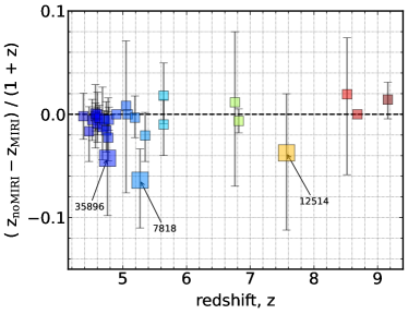
Figure 4: Comparison of the redshifts for galaxies in our sample with and without the MIRI data. The data points show the relative difference between the photometric redshifts (derived from our BAGPIPES fits) for the galaxies excluding MIRI ($z_{\mathrm{noMIRI}}$) and when including MIRI ($z_{\mathrm{MIRI}}$) as a function of the prior photometric redshift from Finkelstein et al. (2022b). Annotated points indicate objects with $\left|z_{\mathrm{noMIRI}}-z_{\mathrm{MIRI}}\right|>0.2$. These objects indicate shifts in their photometric redshift, where at least in part this is because of nebular emission in one or more bands.

Figure 4 compares the redshifts for the galaxies in our sample derived from our BAGPIPES fits for the galaxies excluding the MIRI data ($z_{\mathrm{noMIRI}}$) and when including the MIRI data ($z_{\mathrm{MIRI}}$) as a function of the prior photometric redshift from Finkelstein et al. (2022b). For most galaxies there is good agreement. For completeness we include all 28 galaxies in this comparison, using the photometric-redshifts even for galaxies with spectroscopic redshifts.

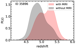
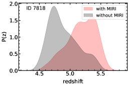
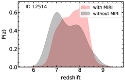
Figure 5: Comparison of redshift posterior probability densities, $P(z)$, derived from the BAGPIPES fits to three of the galaxies in the sample (as labeled). These three galaxies each have a change of more than 0.2 between the median redshift when including the MIRI F560W and F770W data in the fit versus when they are excluded. For the case of galaxy IDs 35896 and 7818, the IRAC$-$MIRI colors are blue, indicating redshifted emission lines (likely H$\beta$+[O iii] and H$\alpha$) inhabit both IRAC bands while the MIRI data probe the galaxy continua. In the case of galaxy ID 12514, the MIRI F560W band clearly shows boosted emission, likely from redshifted H$\alpha$ at $z=7.6-8$.

In several instances we see the median redshift from the posterior shifts appreciably when including the MIRI data (with $\Delta z>0.2$; these are annotated in Figure 4). In all cases the shift in the redshift probability density appears to be related to the effects of one or more emission lines in the IRAC or MIRI passbands. Figure 5 illustrates the shift in $P(z)$ from the BAGPIPES fits for these galaxies.

Two of these galaxies lie at $4<z<6$ (galaxy IDs 35896 and 7818). Adding the MIRI data favors having strong nebular emission in both of the IRAC bands. This occurs at $z\mathrel{\hbox{\hbox to0.0pt{\hbox{\lower 4.0pt\hbox{$\sim$}}\hss}\hbox{$>$}}}5$ when H$\beta$+[O iii] enters the IRAC Ch1 bandpass (at 3.6 µm) and H$\alpha$ enters the IRAC Channel 2 bandpass (at 4.5 µm; see Figure 1). Inspection of the galaxy SEDs (see Fig. Set. 3) shows that the IRAC–to–MIRI colors ($[3.6]-[5.6]$ and $[4.5]-[5.6]$) are blue for both of these galaxies. The BAGPIPES fits that include the MIRI data favor models in which the galaxy has strong nebular emission in the IRAC bands to account for the observed color. This increases (decreases) the redshift probability density at higher (lower) redshifts for these galaxies.

The remaining galaxy, ID 12514, lies at $z\approx 7.7$. Figure 5 shows the redshift probability densities for this galaxy. The MIRI F560W image shows evidence of “boosted” flux compared to the MIRI F770W image (see the images in Fig. 2), where the MIRI color is $[5.6]-[7.7]=-1.1\pm 0.3$ mag (see Table 5). The most likely explanation for this boosted emission appears to be from redshifted H$\alpha$+[N ii] at $z=7.6-8.0$ in the MIRI F560W bandpass (see Fig. 3). The strength of the flux in the F560W bandpass decreases the probability density for redshifts with $z\mathrel{\hbox{\hbox to0.0pt{\hbox{\lower 4.0pt\hbox{$\sim$}}\hss}\hbox{$<$}}}7$ as these would place H$\alpha$ at wavelengths shorter than covered by the bandpass (see Figure 1).

Therefore, nebular emission lines appear to be responsible for the larger shifts in the photometric redshifts. However, these cases are generally exceptions. For most galaxies in the sample the redshift posteriors are consistent, where Fig. 4 shows the differences are negligible in median redshifts with and without including the MIRI data. We expect that many (even most) of the galaxies in the sample also exhibit strong emission lines given the preponderance of evidence from other galaxies at these redshifts (see Section 4.1) and by inspection of the SEDs in Figure 3. In these cases adding the MIRI data supports the redshifts, either because the emission lines make less of an impact on the redshift likelihoods or because the MIRI data reinforce them.

4.3 The Impact of MIRI on the Stellar Masses, Dust Attenuation, and SFRs

Figure 6: Comparison of stellar masses and SFRs derived from the SED modeling for galaxies including the MIRI F560W and F770W data and without the MIRI data. The top set of panels show the comparison for the stellar mass. The bottom set of panels show the comparison for the SFR. In each row the left panel shows the direct comparison, where the dashed line shows the one-to-one relation. The right panel shows the logarithmic difference, defined as $\Delta\log M_{\ast}^{\mathrm{with~{}MIRI}}-\log M_{\ast}^{\mathrm{without~{}MIRI}}$ (similarly for the SFR). The symbols are color-coded by redshift (using the right panel). In the right panel the large rectangular boxes and error bars show the median value (and scatter) in two bins of redshift ($4<z<6$ and $6<z<10$). The values for these are given in Table 3. Adding the MIRI data generally lowers the SFRs and stellar masses of these galaxies though the scatter is significant. The median offset is larger for galaxies at higher redshifts.

Figure 6 compares the stellar masses and SFRs derived for the galaxies in our sample using the simple delayed-$\tau$ models with BAGPIPES for the case where we include the MIRI F560W and F770W data and when we exclude it. In general, including the MIRI data reduces the stellar masses and SFRs for the galaxies.

Table 3: Offsets in Stellar Mass and SFRs for $4<z<10$ galaxies when including the MIRI F560W and F770W data.

	Stellar Mass offsets		SFR offsets
	$\langle\Delta\log M_{\ast}\rangle=$		$\langle$ $\Delta$ log SFR $\rangle=$
	$\log M_{\mathrm{\ast,noMIRI}}/M_{\mathrm{\ast,MIRI}}$		log SFRnoMIRI / SFRMIRI
Sample	Median	Scatter	Median	Scatter
$4<z<6$	0.25 dex	0.28 dex	0.15 dex	0.12 dex
$6<z<10$	0.38 dex	0.44 dex	0.29 dex	0.27 dex

Note. — The quantities with the subscript “noMIRI” denote values derived without the MIRI data. Quantities with the subscript “MIRI” denote the values derived with the 5.6 and 7.7 µm MIRI data. The scatter is the inter-68-percentile interval derived from the median absolute deviation.

We study the offsets in stellar mass and SFR for our galaxies in two redshift bins, $4<z<6$ and $6<z<10$, where the median offsets in stellar mass and SFR are indicated in the Figure 6 as large rectangles, and are listed in Table 3. For this comparison, we have defined $\Delta\log M_{\ast}=\Delta\log M_{\ast}^{\mathrm{with~{}MIRI}}-\log M_{\ast}^{\mathrm{without~{}MIRI}}$ and $\Delta\log\mathrm{SFR}=\log\mathrm{SFR}^{\mathrm{with~{}MIRI}}-\log\mathrm{SFR}^{\mathrm{without~{}MIRI}}$. We have added their uncertainties in quadrature, but this assumes the stellar masses and SFRs derived with and without MIRI are independent. Strictly speaking this is not true as both values use the same HST and Spitzer/IRAC data. Therefore it is likely that the error bars are overestimated assuming the values are correlated. Nevertheless this does not have a major impact on our work because we are interested in the medians and scatter of the sample.

Formally, the offsets in stellar mass are $\Delta\log(M_{\ast})=0.25$ dex for $4<z<6$ and 0.38 dex for $6<z<10$. The inter-68%-tile intervals are 0.28 and 0.44 dex, respectively (estimated using the median absolute deviation, $\sigma_{\mathrm{NMAD}}$). For the SFRs the offsets are $\Delta\log(\mathrm{SFR})=0.15$ dex for $4<z<6$ and 0.29 dex for $6<z<10$, with an inter-68 percentile interval of 0.12 dex and 0.27 dex, respectively. Because the impact of MIRI is larger on the stellar mass than the SFR, the specific SFRs will be increased by approximately $\Delta\log\mathrm{SFR}-\Delta\log M_{\ast}\approx 0.1$ dex (see Table 3).

The reasons for the offsets are similar to that discussed for the individual galaxies in Section 4.1. Including the MIRI data generally favors stellar populations with bluer rest-UV/optical colors, with lower $M/L$ ratios. This forces the constraints to lower stellar-mass models. For the SFRs, because the colors are bluer, there is less dust attenuation favored in the models, which lowers the SFRs compared to models with higher dust attenuation (at fixed observed galaxy luminosity). The MIRI data also remove some of the degeneracy between models with redder stellar populations versus those with strong emission lines impact select bands. These have the combined effect of favoring lower stellar masses and SFRs when including the MIRI data.

There is significant scatter in the offsets of stellar mass and SFR for individual objects. In Figure 6 the error bars on the large rectangles show the inter-68-percentile range (i.e,. the difference between the 16–84 percentiles) for both the $4<z<6$ and $6<z<10$. For some galaxies the offsets are insignificant, with $\Delta\log M_{\ast}\approx 0$ and $\Delta\log\mathrm{SFR}\approx 0$. In other words, in some cases the MIRI data support the range of stellar population parameters favored by the fits to the HST/ACS + WFC3 and Spitzer/IRAC data, but the MIRI data improve the accuracy of the measurements, typically by a factor of order two.

In most cases the MIRI data reduce the stellar mass and SFRs, in some cases substantially. Figure 6 shows that this is generally the case, where the MIRI data decrease the average stellar mass and SFR for galaxies in our sample, typically by a factor of order two. We will explore the implications this has on the evolution of the galaxy stellar-mass density in Section 5.

4.4 The Impact of MIRI on the Inferred Star-Formation History (and the Mass Formed in Bursts)

Using the results from Section 3, we also explored the possibility that an early burst of star formation could contribute stellar mass to the galaxies in our sample, and how the JWST/MIRI data can improve the constraints on this population. For this study, we used the SED fits to the galaxies in our sample using a star-formation history that includes both the delayed-$\tau$ model and the burst of stars formed at $z_{f}=100$. The details of the other model parameters are listed in Table 2.

To quantify the amount of allowed stellar mass formed in the burst for each galaxy, we use the Bayesian Information Criterion (BIC, Bailer-Jones 2017). The BIC provides a criterion for model selection in the case that one introduces a model with an additional parameter. In our case we are selecting between between two models, one with a star-formation history that has a delayed-$\tau$ model only, and one with both the delayed-$\tau$ model and an early burst at $z_{f}=100$. When comparing the two models, the BIC applies a penalty term for the additional parameter to determine if the additional parameter improves the fit, or is overfitting the data.

We use the BIC defined as (e.g., Buat et al. 2019),

$$\mathrm{BIC}=\chi_{0}^{2}~{}\times~{}k\ln N,$$ (2)

where $\chi_{0}^{2}$ is the minimum chi-squared from the SED-fitting, $k$ is the number of independently fitted parameters (we use $k=7$) and $N$ is the number of data points ($N=8$ or 10, depending on if the MIRI [5.6] and [7.7] data are included or not).

Figure 7: Example fits to SEDs for the galaxies in our sample, comparing the results from fits that include an early burst of star-formation at $z_{f}=100$. Data points and upper limits have the same definitions as in Figure 3. In each panel, the shaded regions show the stellar population fit to the SED using the total model (cyan-shaded = delayed$-\tau$ plus the burst) and delayed-$\tau$ model only (gray-shaded, these are identical to those in Figure 3; there is almost no difference between the cyan- and gray-shaded models). The tan-shaded region shows the light permitted in the burst component. The labels indicate the amount of stellar mass in each component. Each row shows the results for one galaxy, where the Left panel shows the results that exclude the MIRI F560W and F770W data, and the tight panel shows the results including the MIRI F560W and F770W data. The complete figure set (28 images) is available online.

Fig. Set7. SED fits including the MIRI data and excluding the MIRI data for all galaxies comparing the fits with and without bursts at $z_{f}=100$.

Our goal is to quantify the upper limit on the stellar mass formed in an early burst that could exist in our galaxies. To do this, we select models with bursts ($z_{f}=100$) that are not excluded by the BIC criterion. That is, for a given galaxy we identify all models that satisfy $\chi^{2}\leq\mathrm{BIC}$, where the BIC is defined in Equation 2, and $\chi^{2}$ is the fit for a given model (this is similar to the approach adopted by Buat et al. 2019). For each galaxy, we select the model with the highest stellar mass in the $z_{f}=100$ burst from the subset of models that satisfy the BIC. We then take this as an upper limit on the stellar mass permitted in the burst. Comparing this upper limit on the stellar mass formed in bursts to the range of stellar masses from the fits we find that the limiting stellar mass from models that satisfy the BIC criteria corresponds roughly to a 99.7% upper limit on the mass (i.e., the values we report correspond approximately to a $3\sigma$ upper limit on the stellar mass). Tables 6 and 7 list the upper limit on the stellar mass in the burst component for all galaxies in the sample for the case that we include and exclude the MIRI data, respectively.

Figure 7 shows example SED fits for galaxies in our sample, both with and without the bursts, for both of the the cases that we include and exclude the MIRI 5.6 and 7.7 µm data. The complete figure set (28 images) is available online. The examples shown in the Figure include a galaxy where the IRAC data are bright relative to the MIRI data (ID 18441). In this case, without the MIRI data the allowed stellar mass in the burst can reach $\log M_{\ast}/M_{\odot}$ = 11.0, but adding MIRI reduces this by nearly an order of magnitude. For galaxy ID 7364, the MIRI data favor red IRAC–to–MIRI colors. Nevertheless, because the MIRI data constrain the models at longer wavelengths, they also lower the amount of stellar mass allowed in the burst: without the MIRI data the burst can include $\log M_{\ast}/M_{\odot}=10.9$; when MIRI data are included the mass in the burst declines by 0.3 dex (a factor of two). For galaxy ID 6811, the MIRI data show that because they constrain the SED at longer wavelengths, the amount of stellar mass allowed in the burst is reduced by a factor of 0.6 dex (nearly a factor of five).

Figure 8: Comparison of stellar masses derived for galaxies with and without early bursts (at $z_{f}=100$). The top row shows the results that lack MIRI data. The top-left panel shows the stellar masses derived from the delay-$\tau$ models only (labeled “no burst”) compared to the models that include the burst (labeled “allowed in burst”). The top-right panel shows the difference between the stellar masses as a function of redshift. The bottom row shows the same results for the galaxies including the MIRI data. In the left panels, the dashed lines show the one-to-one relation and the solid lines show the median offsets. In the right panels, the large rectangles show the medians in two bins of redshift ($4<z<6$ and $6<z<9$) these are given in Table 4. Adding the MIRI data reduces the amount of stellar mass allowed in the burst components.

Table 4: Ratio of the stellar mass allowed in models that include an early burst of star-formation (at $z_{f}=100$) to those that include only a delayed$-\tau$ model.

	$\log M_{\mathrm{\ast}}(with~{}burst)-\log M_{\mathrm{\ast}}(no~{}burst)$
	with MIRI data		no MIRI data
Sample	Median	Scatter	Median	Scatter
$4<z<6$	0.59 dex	0.16 dex	0.87 dex	0.23 dex
$6<z<10$	0.69 dex	0.04 dex	1.11 dex	0.13 dex

Note. — The values labeled “with burst” denote the upper limit on the stellar mass for models that include bursts. The values labeled “no burst” denote the stellar masses for models that assume only a delayed-$\tau$ star-formation history. The values “with MIRI” include the 5.6 and 7.7 µm flux densities from MIRI.

The addition of the MIRI F560W and F770W data reduces the amount of stellar mass that can form in early bursts. Figure 8 shows the change in stellar mass for the case that the star-formation histories include only delayed-$\tau$ models (labeled “no burst” in the figure) compared to when an early burst of star formation at $z_{f}=100$ is included (labeled “allowed in burst” in the figure). Figure 8 shows the results for both the case that the MIRI data are excluded (top row) and when the MIRI data are included (bottom row). For the fits that lack MIRI data, the amount of stellar mass allowed in the burst is nearly an order of magnitude higher than constrained in the delayed-$\tau$ models: in this case the median differences in the log of the stellar mass of the models with early bursts and those with only delayed-$\tau$ models is 0.9 dex at $4<z<6$ and 1.1 dex at $6<z<9$. For the fits that include the MIRI data, the amount of stellar mass allowed in the bursts is significantly reduced: the median differences in this case are 0.6 dex at $4<z<6$ and 0.7 dex at $6<z<9$. These values are listed in Table 4.

5 Discussion

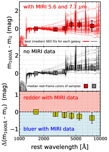
Figure 9: Comparison of median, relative SED for each galaxy, both for the case that MIRI data are used (top panel) and when the MIRI data are excluded (middle panel). The individual lines are the median SED model fit to each galaxy in the sample, shifted to the rest-frame. The large data points show the median rest-frame magnitude at 1600 Å, 2800 Å, and $U$, $B$, $V$, and $I$. The error bars show the scatter in the sample. All models have been normalized to the 1600 Å magnitude (which accounts for the lack of scatter at that wavelength). The bottom panel shows the difference in color ($\Delta m$) between the models with and without the MIRI data. The error bars show the range of the 16th-84th percentiles of the sample. The change in the color at the reddest wavelengths probed (about the rest-frame $I$-band) corresponds to a $\Delta m\approx 0.4$ mag.

5.1 On the Colors, Stellar Masses, and Nebular Emission in Early Galaxies

One of main findings in this paper is that the MIRI data favor bluer colors in galaxies at $4<z<9$. Figure 9 shows this by comparing the relative SED for each galaxy, both in the case of including the MIRI data and without the MIRI data. Including the MIRI data reduces the derived rest-frame $I$-band light by approximately $\Delta m_{\mathrm{1600~{}\AA}}-I\approx 0.4$ mag. Inspecting Figure 9 this appears to result from many galaxies favoring bluer SEDs when the MIRI data are included. In other words, without the MIRI data, the SED is unconstrained at longer wavelengths, and this allows for a greater range of SED shape (where the median favors a solution which on average is redder). Adding the MIRI data shifts the likelihood to bluer populations for many galaxies. This has a major impact on the implied $M/L$, as the blue rest-frame colors imply younger ages, lower dust attenuation, or both. The fact that adding the MIRI data makes the galaxies bluer largely explains the differences in the derived stellar masses and SFRs observed in Figure 6, where adding the MIRI data lowers the stellar masses and SFRs compared to when the MIRI data are excluded.

Therefore, our interpretation of the MIRI data is that galaxies at high redshifts ($z>4$) are bluer than inferred from previous studies. This adds to other studies that find that galaxies at high redshifts must have (very) blue colors. Studies from the pre-JWST era argued that galaxies at $z>4$ show indications of declining (i.e., steepening) UV spectral slopes with increasing redshift (e.g., Bouwens et al. 2012; Finkelstein et al. 2012; Wilkins et al. 2016; Bhatawdekar & Conselice 2021). These conclusions have been reinforced by early JWST imaging that shows very blue colors among UV-selected galaxies (e.g., Nanayakkara et al. 2022; Topping et al. 2022). We find here that including the MIRI 5.6 and 7.7 µm data provides strong evidence that the stellar populations are very blue in their rest-frame UV–to–$I$-band colors, seemingly more so than inferred from these previous studies (as in some cases the galaxies in our sample are identical to those in these other studies). Therefore, the MIRI data favor lower stellar masses and lower SFRs in distant galaxies.

Adding the MIRI data also changes the interpretation of the strength of nebular emission in the galaxies in the sample. Many of the galaxies show red colors between the HST/WFC3 and Spitzer/IRAC data (Figure 3). In the absence of MIRI data, the SED fitting interprets these colors as a combination of higher dust obscuration, older ages, and strong nebular emission. This has been reported previously for individual galaxies and for stacked samples at $z>6$ (e.g., Castellano et al. 2017; Stark et al. 2017; De Barros et al. 2019; Hutchison et al. 2019; Endsley et al. 2021; Stefanon et al. 2022). The fact that without the MIRI data the models allow for higher dust obscuration and older stellar populations increases the $M/L$ and the stellar masses. The higher dust obscuration also leads to higher SFRs. However, including the MIRI data changes this interpretation for the galaxy population. Nebular emission lines appear to be the primary explanation for the red HST/WFC3 to Spitzer/IRAC colors (while there are some galaxies where the MIRI data does not change [e.g., galaxy IDs 6811 and 7364 in Figure 3] this does not change the main result in general). This means (1) the nebular emission lines for high redshift galaxies must be strong and (2) the stellar populations are blue. Early JWST results show emission lines remain strong in high-redshift galaxies and impact the reddest ($4-5$ µm) bandpasses in NIRCam (e.g., Endsley et al. 2022; Giménez-Arteaga et al. 2022; Santini et al. 2022b; Topping et al. 2022; Whitler et al. 2022). The MIRI data appear necessary to extend the rest-frame wavelength coverage to $>$7000 Å, past the strongest of the nebular emission features in the rest-frame optical.

5.2 Implications for Early Star-Formation and Stellar Masses in Galaxies

The difference between the delayed-$\tau$ star-formation history and the model that includes bursts, while simplistic, arguably spans the gamut of available star-formation histories of galaxies. Simulations show that galaxies experience many discrete bursts, but when averaged over long time baselines the evolution is mostly smooth (e.g., Diemer et al. 2017; Iyer et al. 2019; Leja et al. 2019). Therefore the smoothly evolving delayed-$\tau$ model represents the slowly evolving evolution of galaxy star-formation histories. This can reproduce the bluest colors (and lowest $M/L$) of the stellar population. Of course, galaxies can experience a host of stochastic bursts through changes in gas accretion or events that can cause sudden changes in the star formation, possibly as a result of mergers (e.g., Kartaltepe et al. 2022), or from the onset of strong feedback from an AGN (e.g., Wagner et al. 2016). “Bursts” of star-formation from these events will add stellar mass, but if these occur at $z<100$ then they will be younger, and will have $M/L$ lower than a model with a burst at $z_{f}=100$. As such, the models with a burst at $z_{f}=100$ have the maximum $M/L$ and the oldest possible ages for a stellar population at the observed redshift of each galaxy. For these reasons, the models with this burst represent a maximum stellar mass possibly formed in these galaxies.

An advantage of focusing on galaxies at high redshifts is that the amount of time for discrete episodes of star-formation (i.e., many individual bursts) is small given the age of the Universe is 1 Gyr at $z=5.7$ and 500 Myr at $z=9.6$ for the adopted cosmology. This is shorter than the lifetimes of stars of spectral type A and later. The short age of the Universe limits the maximum $M/L$ for stellar populations in these galaxies. Combined with longer wavelengths probed by the MIRI 5.6 and 7.7 µm data, this allows us to place tighter constraints on the mass from earlier bursts in high redshift galaxies than has been possible previously.

Using the MIRI data, we find that the maximum stellar mass from bursts for the galaxies in our sample is lower by 0.6 dex at $4<z<6$ and 0.7 dex at $6<z<9$ (see Table 4). Furthermore, our results show that including MIRI reduces the amount of stellar mass allowed in these models, by an order of magnitude in some cases. In itself this is interesting as nearly all galaxies show no direct evidence for such early star-formation. Comparing the median stellar masses of galaxies when fit by the delayed-$\tau$ models only and those with the delayed-$\tau$ models and the early burst at $z_{f}=100$ shows they differ by $\mathrm{median}(\Delta M_{\ast})\approx 0.1$ dex, and the 16th-to-84th percentile range also is similar (see the plots in Figure 7). We find no convincing cases in our sample where the galaxies require a burst at $z_{f}=100$ to better fit their SEDs. This would imply that galaxies do not experience early bursts of star-formation (or at least such bursts do not form sufficient mass that we require them).

We can compare our results for $4<z<9$ galaxies to those at lower redshifts. For example, Papovich et al. (2001) found that with $K$-band data for $z\sim 2-3.5$ galaxies, early bursts could contain between 3 and 8 times the stellar mass of the younger populations that dominated the SED in those galaxies. The $K$-band is roughly the same rest-frame wavelength for galaxies at $z\sim 2$ as MIRI is for galaxies at $z\sim 8$. With MIRI we find that the stellar mass in an early burst can be $\sim 4-5\times$ the stellar mass of the younger population in $4<z<9$ galaxies. The early burst mass is modestly lower than the results from Papovich et al. (2001). The reason for this is a combination of effects. At $4<z<9$, the galaxies are blue, so they can hide more stellar mass in an early burst. However, because the universe is younger at $4<z<9$, any early burst of stars is also younger, with a lower $M/L$ and therefore a lower stellar mass. These effects offset, leading to only a modest difference in the amount of stellar mass that could be contained in bursts. Nevertheless, this highlights the importance of probing the SEDs of galaxies at rest-frame wavelengths longer than $\sim$5000-7000 Å to constrain these populations.

Part of our findings could be impacted by biases and limitations. First there is selection bias: all the galaxies studied here were selected in HST/WFC3 data, and therefore required some rest-frame UV emission above the HST/WFC3 detection limit. It will be important to test if there is evidence for early episodes of star-formation in galaxies with future JWST observations. This will be potentially very important for red galaxies, including JWST/NIRCam-selected galaxies that lack HST counterparts (Glazebrook et al. 2022; Pérez-González et al. 2022). Second, very recent work shows evidence for older stellar populations in the spatially resolved colors of $6<z<9$ galaxies (Giménez-Arteaga et al. 2022). As these issues become better constrained, then the ages of the stellar populations in distant galaxies could begin to inform us about when galaxies first form stars (see Whitler et al. 2022).

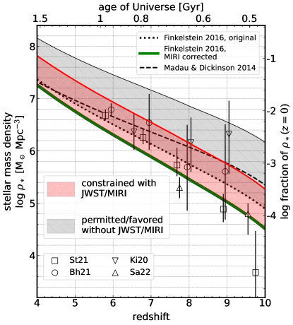
Figure 10: Evolution of the cosmic stellar mass density, $\rho_{\ast}$, in galaxies from $4<z<10$. The lines show pre-JWST constraints from Finkelstein (2016) and Madau & Dickinson (2014). The data points show recent measurements of $\rho_{\ast}$ at $z>6$ from the literature (Kikuchihara et al. 2020 [Ki20], Bhatawdekar & Conselice 2021 [Bh21], Stefanon et al. 2021 [St21], Santini et al. 2022a [Sa22]), which largely follow the pre-JWST constraints. The shaded regions show maximally allowable stellar mass density assuming galaxies experience a burst at $z=100$ followed by “normal” star-formation. Constraints lacking JWST/MIRI coverage to rest-frame 1 µm allow for a stellar mass density that is up to 0.8 dex higher at $z=4$ and 1.4 dex higher at $z=10$. Including MIRI 5.6 and 7.7 µm data lowers the maximum allowed by up to a factor of 5.

5.3 Implications for Galaxy Growth

The question of how much mass is contained in galaxies is related to the integral of the galaxies’ star-formation histories. This is important because it contains the integrated record of how rapidly galaxies acquire their baryons, and how efficiently they convert these into stars. This has already been discussed as an impossibly early galaxy problem, where galaxies may have acquired too much stellar mass: in typical JWST surveys galaxies should have less stellar mass than a few times $10^{11}$ $M_{\odot}$ (Behroozi & Silk 2018; Boylan-Kolchin 2022).

The effect of adding the MIRI data already is that the stellar masses and SFRs derived for galaxies tend to be overestimated when such data are excluded. The median offsets for the galaxies in our sample are 0.15 dex at $4<z<6$ and rise to $\approx$0.3 dex at $6<z<9$ (Figure 6 and Table 3). Assuming that these (median) offsets apply to previous estimates of galaxy stellar masses, then it implies that measurements of the cosmic SFR density (SFRD, which is the average SFR in all galaxies per co-moving volume element) are similarly biased to higher values at these redshifts.

Figure 10 shows the impact of these lower SFRs on the cosmic stellar-mass density, $\rho_{\ast}$. Firstly, the figure shows $\rho_{\ast}$ derived from the integral of the SFRD for two empirical models calibrated against measurements from the literature (Madau & Dickinson 2014; Finkelstein 2016). Finkelstein (2016) shows that these models are consistent with a compilation of measurements of $\rho_{\ast}$ from the literature at $4<z<10$ prior to the launch of JWST, (Oesch et al. 2014; Duncan et al. 2014; Grazian et al. 2015; Song et al. 2016). The thick line in Figure 10 labeled “MIRI corrected” shows the empirical model of Finkelstein corrected by the offsets of the SFRs derived in Table 3. To derive these corrections we have interpolated the results from Table 3 assuming median redshifts of $z=5$ and 8 for the derived offsets in the two redshift bins. Although we use the offsets derived from the SFRs, using those for the stellar masses changes the results by $\approx$0.1 dex. We note, however, that because the MIRI data imply offsets in the SFRs of galaxies, they similarly lower the values of the cosmic SFRD at $z>4$.

Secondly, the MIRI data improve the constraints on the amount of stellar mass possible in early bursts of star-formation (Section 4.4). This is illustrated by the shaded regions in Figure 10. To derive the area in the shaded swaths, we applied the ratio between the mass permitted in early bursts at $z_{f}=100$ to the fiducial value (listed in Table 4), and interpolated them over redshift as above. Therefore, the effects of adding the MIRI data both lower SFR (and stellar masses) and limit the total stellar mass allowed in early bursts. The combination of these effects reduces the upper bound on the total cosmic stellar mass density allowed by the data by 0.4 dex at $z=4$ and by 1.0 dex at $z=9$. As illustrated in Figure 10, this implies that the JWST/MIRI data have constrained the stellar mass in galaxies at $z=9$ to be less than 0.1% that of the present-day value ($\rho_{\ast}(z=0)$).

5.4 Implications for the Nature of Early Galaxies

The fact that galaxies have bluer colors than inferred from previous constraints has other consequences (i.e., they are “bluer than they appear”). Our findings dovetail with other recent results from JWST NIRCam imaging. The results in this Paper are likely only the first foray into the properties of distant galaxies using the longer wavelength data available from MIRI. Future studies will be able to combine both NIRCam and MIRI imaging, providing JWST–quality data from $0.8-10$ µm, with NIRSPec spectroscopy, which will improve the constraints presented here. Already there are indications that using JWST/NIRCam data only that the number density of luminous galaxies at $z>10$ may be much higher than predictions (e.g., Bouwens et al. 2022; Donnan et al. 2022; Finkelstein et al. 2022a; Harikane et al. 2022; Naidu et al. 2022; Robertson et al. 2022). One interpretation of these discoveries is that the UV–luminosity per unit stellar mass (the UV “efficiency”) may be higher than models predict. This could be a result of changes in the stellar populations such that they produce more ionizing photons per unit mass. This is expected both for the case that the galaxies contain high-mass, very metal-poor stars (Olivier et al. 2022) or if their stellar populations have an IMF weighted toward high-mass stars (Raiter et al. 2010). Importantly, either of these effects would further decrease the $M/L$ ratio of the stellar poplation, and thus lead to even lower stellar masses than we have measured with the MIRI data. Therefore, it will be important to constrain the nature of the stars in these galaxies. In the meantime, the MIRI data have better constrained the available light in stars at these early epochs, finding that they contain at least three times less “light” at rest-frame $0.7-1$ µm than previously known.

6 Conclusions

In this Paper we have presented results from CEERS on the stellar population parameters for 28 galaxies with redshifts $4<z<9$ using new imaging data from JWST/MIRI at 5.6 and 7.7 µm. Our galaxy sample was detected in deep data from HST/WFC3 and ACS and has observations from Spitzer/IRAC at 3.6 and 4.5 µm. The MIRI 5.6 and 7.7 µm data extend the coverage of the rest-frame spectral energy distribution to nearly 1 micron for galaxies in this redshift range. We use these data to study the improvements in the stellar masses and SFRs of the galaxies at these redshifts when the MIRI data are included. Our main results are the following.

1. Galaxies at $4<z<9$ have bluer rest-frame UV–$I$-band colors ($m_{\mathrm{1600~{}\AA}}-I$) when using the MIRI data compared to when they are excluded. Using the MIRI data we model the SEDs using stellar population synthesis models (with BAGPIPES). When we compare the average galaxy SED (Figure 9) we find that models that include the MIRI data are (on average) $\Delta(m_{\mathrm{1600~{}\AA}}-I)\approx 0.4$ mag bluer in their rest-frame colors compared to models that exclude the MIRI data.

2. Galaxies generally have lower stellar masses and SFRs when the MIRI data are included. For the majority of the galaxies (Figure 6) adding the MIRI data reduces the derived stellar masses by 0.25 dex at $4<z<6$ and by 0.38 dex at $6<z<9$ . Similarly including the MIRI data reduces the SFRs by 0.15 dex at $4<z<6$ Because the impact is larger on the stellar masses than on the SFRs, the specific SFRs will be increased by approximately $\Delta\log\mathrm{SFR}-\Delta\log M_{\ast}\approx 0.1$ dex when the MIRI data are included.

   There are multiple reasons the stellar masses and SFRs are lowered when we include the MIRI data. The first reason is that the galaxies are blue, and the fits favor models with lower dust attenuation and models with lower $M/L$ in general. The second reason is that in many cases the IRAC 3.6 and 4.5 µm data probe the rest-frame optical, and these show indications of containing light from strong emission lines (e.g., redshifted H$\beta$ + [O iii], H$\alpha$+[N ii], [O ii], etc.). These boost the flux in these bands. In the absence of MIRI data the models can not determine if the red rest-frame UV-optical colors are a result of dust attenuation, older stellar populations, or strong emission lines (or all of them). The parameter constraints then give more weight (probability density) to models with higher stellar masses and SFRs. When the MIRI data are included, they probe more of the stellar continuum at $>$7000 Å rest-frame. The model fits that include the MIRI data then show the dominant effect in the rest-frame optical are strong nebular emission lines. This problem will persist for models that use NIRCam data as it also is limited to wavelengths less than 5 µm, but this can be tested with forthcoming datasets.

3. The amount of stellar mass that could have formed in early bursts is lower. We estimated the amount of stellar mass formed by using a star-formation history that includes an early burst (at $z_{f}=100$) in addition to a smoothly evolving component. A stellar population formed at this early time would fade and redden with time, and it would have the highest $M/L$ at any subsequent time and therefore represents an upper limit on the amount of mass that could exist in these galaxies. The MIRI data improve the constraint on this stellar population by probing longer wavelengths where the impact from this stellar population is more pronounced. Figure 8 shows that without the MIRI data, the amount of stellar mass in this population can be as much as 0.9 dex higher at $4<z<6$ and as much as 1.1 dex higher at $6<z<9$ . Including the MIRI data, these drop to 0.6 dex at $4<z<6$ and 0.7 dex at $6<z<9$ . Therefore, adding the MIRI reduces the amount of mass in early bursts by a factor of order 2 compared to when no MIRI data are used.

4. Our analysis of the MIRI 5.6 and 7.7 µm therefore provides evidence that there is less star-formation in distant galaxies than found in previous studies, because the SFRs and stellar masses are lowered. The MIRI data also reduce the limits on the amount of stellar mass possibly formed at early times. The combination of these results has implications for the evolution of the cosmic stellar-mass density, $\rho_{\ast}$. We showed (Figure 10) that applying our results lowers the amount of stellar mass density in galaxies at $z=9$ to be less than 0.1% of the present day, $z=0$, value. This is an order of magnitude lower than implied by previous studies (i.e,. pre-JWST).

Table 5: Observed Properties of the Galaxy Sample

. ID R.A. (J2000) Decl. (J2000) F160 E160 F560 E560 F770 E770 $z_{\mathrm{phot}}$ $z_{\mathrm{16}}$ $z_{\mathrm{84}}$ $z_{\mathrm{spec}}$ $\mathcal{P}(z=4)$ $\mathcal{P}(z=5)$ $\mathcal{P}(z=6)$ $\mathcal{P}(z=7)$ $\mathcal{P}(z=8)$ $\mathcal{P}(z=9)$ (deg) (deg) $\mathrm{nJy}$ ($\mathrm{nJy}$) ($\mathrm{nJy}$) ($\mathrm{nJy}$) ($\mathrm{nJy}$) ($\mathrm{nJy}$) 5090 215.04973 52.89656 102.0 12.5 158.8 17.9 148.0 14.4 4.38 4.18 4.56 -1.000 0.68 0.27 0.00 0.00 0.00 0.00 11329 215.04086 52.90623 49.4 6.9 63.5 20.4 44.5 15.7 4.47 4.15 4.65 -1.000 0.55 0.39 0.00 0.00 0.00 0.00 34813 214.97597 52.920297 82.2 16.2 67.0 16.7 43.9 19.4 4.52 4.17 4.59 -1.000 0.52 0.36 0.00 0.00 0.00 0.00 7600 215.04415 52.898731 564.7 29.4 3283.1 32.4 4101.7 24.8 4.57 4.13 4.65 -1.000 0.62 0.38 0.00 0.00 0.00 0.00 13389 215.03793 52.909329 453.9 29.7 578.3 26.9 661.0 22.0 4.57 4.43 4.61 -1.000 0.38 0.61 0.00 0.00 0.00 0.00 37703 214.99094 52.924279 116.7 11.8 278.9 30.4 61.0 17.5 4.60 4.47 4.70 -1.000 0.22 0.78 0.00 0.00 0.00 0.00 15445 215.02689 52.907215 124.5 14.4 187.8 20.2 116.6 14.9 4.60 4.21 4.84 -1.000 0.24 0.62 0.00 0.00 0.00 0.00 41564 214.98708 52.912734 266.4 13.4 481.6 20.8 276.8 15.7 4.63 4.56 4.71 -1.000 0.03 0.97 0.00 0.00 0.00 0.00 45145 215.00878 52.919869 101.2 15.2 108.6 29.6 69.0 19.3 4.68 4.37 5.20 -1.000 0.15 0.74 0.03 0.00 0.00 0.00 14913 215.02081 52.901523 78.3 14.1 72.8 17.8 9.4 8.9 4.68 4.47 4.94 -1.000 0.19 0.81 0.00 0.00 0.00 0.00 42638 214.97762 52.90349 547.0 31.8 711.4 28.5 596.3 23.4 4.71 4.57 4.77 -1.000 0.02 0.90 0.00 0.00 0.00 0.00 41375 215.00283 52.924312 109.2 15.4 47.2 18.1 119.1 14.8 4.74 4.60 5.13 -1.000 0.07 0.92 0.01 0.00 0.00 0.00 35896 214.98522 52.924266 96.3 10.2 114.5 14.8 110.0 15.3 4.76 4.35 5.33 -1.000 0.06 0.73 0.07 0.00 0.00 0.00 13179 215.04260 52.911968 736.4 23.7 1355.2 26.8 1519.1 21.5 4.78 4.72 4.91 -1.000 0.00 1.00 0.00 0.00 0.00 0.00 19180 215.03170 52.919632 773.3 35.6 749.1 26.0 787.7 19.0 4.93 4.86 4.95 5.077^† 0.00 1.00 0.00 0.00 0.00 0.00 37653 214.99190 52.925053 103.1 12.5 154.0 22.2 108.4 18.5 4.95 4.72 5.59 4.899^‡ 0.06 0.71 0.22 0.00 0.00 0.00 18449 215.02314 52.912683 69.0 10.0 185.0 24.2 165.3 17.6 5.05 4.30 5.57 -1.000 0.14 0.59 0.20 0.00 0.00 0.00 41545 215.00312 52.924103 384.9 18.3 749.2 21.5 656.6 17.5 5.19 5.02 5.44 -1.000 0.00 0.90 0.10 0.00 0.00 0.00 7818 215.02758 52.887744 289.9 21.4 421.4 24.5 399.5 20.9 5.27 4.74 5.46 -1.000 0.02 0.86 0.12 0.00 0.00 0.00 12773 215.03057 52.902606 56.4 12.2 17.0 7.5 71.0 14.1 5.35 4.87 5.43 -1.000 0.00 0.90 0.09 0.00 0.00 0.00 24007 214.95185 52.928275 47.1 4.9 107.8 18.8 56.7 12.6 5.64 5.16 5.79 -1.000 0.00 0.46 0.51 0.00 0.00 0.00 49365 215.00994 52.910669 143.9 14.1 408.5 26.8 541.0 20.6 5.64 5.03 5.82 -1.000 0.01 0.38 0.50 0.00 0.00 0.00 18441 215.03209 52.918972 97.2 11.5 199.6 28.2 169.9 22.0 6.76 5.88 7.24 -1.000 0.00 0.01 0.36 0.48 0.07 0.00 39096 214.98901 52.919652 64.1 8.7 159.5 17.0 57.7 11.2 6.82 6.67 7.08 -1.000 0.00 0.00 0.02 0.97 0.01 0.00 12514 215.03716 52.906712 71.6 13.2 142.3 17.8 50.4 13.6 7.57 6.90 8.41 -1.000 0.00 0.00 0.02 0.39 0.44 0.13 7364 215.03561 52.892208 292.6 17.5 575.7 28.4 611.4 23.1 8.52 7.47 8.68 -1.000 0.00 0.00 0.00 0.17 0.52 0.31 6811 215.03538 52.890666 314.5 13.3 426.8 21.6 404.0 16.9 8.93 8.60 9.05 8.683^∗ 0.00 0.00 0.00 0.00 0.08 0.92 26890 214.96754 52.932966 133.3 8.9 101.9 21.4 60.8 16.8 9.16 8.46 9.24 -1.000 0.00 0.00 0.00 0.00 0.06 0.83

Note. — References for spectroscopic redshifts: ^‡ Stawinski, S., et al., in prep; ^† WERLS; ^∗Zitrin et al. (2015).

Table 6: Derived Stellar masses, SFRs, and Redshifts including the MIRI [5.6] and [7.7] data.

	redshift			$\log M_{\ast}/M_{\odot}$ (dex)			$\log\mathrm{SFR}/M_{\odot}~{}\mathrm{yr}^{-1}$ (dex)			“Burst” Mass
ID	$z_{50}$	$z_{16}$	$z_{84}$	$\log M_{50}$	$\log M_{16}$	$\log M_{84}$	log SFR50	log SFR16	log SFR84	$\log M_{\ast}/M_{\odot}$ (dex)
(1)	(2)	(3)	(4)	(5)	(6)	(7)	(8)	(9)	(10)	(11)
5090	4.33	4.19	4.45	9.01	8.84	9.16	0.59	0.50	0.69	9.55
6811	…	…	…	9.76	9.57	9.88	1.60	1.49	1.72	10.34
7364	8.07	7.35	8.55	9.91	9.72	10.04	1.70	1.57	1.82	10.61
7600	4.41	4.22	4.56	10.54	10.36	10.65	2.09	1.97	2.20	10.93
7818	5.19	4.93	5.39	9.51	9.30	9.64	1.19	1.10	1.29	10.23
11329	4.45	4.31	4.59	8.48	8.14	8.73	0.27	0.17	0.37	9.17
12514	7.69	7.03	8.21	8.78	8.47	9.02	0.70	0.53	0.85	9.45
12773	5.08	4.91	5.24	8.01	7.78	8.24	0.08	-0.18	0.30	8.87
13179	4.79	4.73	4.86	10.07	9.86	10.20	1.71	1.60	1.83	10.57
13389	4.53	4.45	4.60	9.61	9.42	9.75	1.25	1.15	1.37	10.16
14178	4.89	4.76	5.08	8.54	8.29	8.79	0.54	0.35	0.67	9.16
15445	4.59	4.46	4.71	8.92	8.67	9.11	0.63	0.54	0.73	9.36
18441	6.54	5.90	7.11	9.32	9.12	9.46	1.03	0.90	1.17	10.00
18449	4.97	4.43	5.32	9.17	8.93	9.32	0.81	0.67	0.95	9.83
19180	…	…	…	9.72	9.48	9.90	1.54	1.38	1.68	10.14
24007	5.36	5.17	5.52	8.76	8.48	8.91	0.41	0.32	0.53	9.59
26890	8.80	8.61	8.97	8.79	8.46	9.04	0.84	0.50	0.97	9.45
34813	4.38	4.27	4.50	8.26	7.97	8.62	0.33	0.02	0.46	8.97
35896	5.13	4.82	5.40	8.92	8.67	9.08	0.63	0.51	0.76	9.44
37653	…	…	…	8.95	8.58	9.13	0.66	0.53	0.83	9.57
37703	4.63	4.53	4.71	8.41	8.20	8.86	0.47	0.23	0.65	9.21
39096	6.78	6.68	6.87	8.81	8.48	8.98	0.63	0.52	0.75	9.41
41375	4.79	4.66	4.96	8.54	8.27	8.77	0.51	0.34	0.61	9.15
41545	5.13	5.00	5.25	9.80	9.62	9.89	1.38	1.29	1.49	10.32
41564	4.66	4.59	4.74	9.36	9.08	9.52	1.05	0.93	1.17	9.78
42638	4.70	4.64	4.76	9.65	9.39	9.80	1.34	1.20	1.45	10.12
45145	4.72	4.55	4.96	8.59	8.28	8.83	0.51	0.34	0.61	9.52
49365	5.31	5.14	5.52	9.63	9.43	9.75	1.29	1.18	1.42	10.23

Note. — (1) Galaxy ID; (2)–(4) redshift median (50%-tile), and 16th and 84th-percentiles; galaxies with no redshift use the spectroscopic redshift in Table 5; (5)–(7) stellar mass (50th percentile), and 16th and 84th–percentiles in the delayed-$\tau$ model; (8)–(10) SFR median (50th percentile), and 16th and 84th percentiles (all SFRs are averaged over the past 100 Myr) in the delayed-$\tau$ model; (11) maximum stellar mass allowed in the “burst” formed at $z_{f}=100$, these satisfy the BIC criteria (equation 2 in Section 4.4) and correspond approximately to a 3$\sigma$ upper limit.

Table 7: Derived Stellar masses, SFRs, and Redshifts excluding the MIRI data.

	redshift			$\log M_{\ast}/M_{\odot}$ (dex)			$\log\mathrm{SFR}/M_{\odot}~{}\mathrm{yr}^{-1}$ (dex)			“Burst” Mass
ID	$z_{50}$	$z_{16}$	$z_{84}$	$\log M_{50}$	$\log M_{16}$	$\log M_{84}$	log SFR50	log SFR16	log SFR84	$\log M_{\ast}/M_{\odot}$ (dex)
(1)	(2)	(3)	(4)	(5)	(6)	(7)	(8)	(9)	(10)	(11)
5090	4.32	4.17	4.46	9.08	8.75	9.26	0.61	0.50	0.74	10.00
6811	-1.00	-1.00	-1.00	9.85	9.47	10.12	1.70	1.43	1.98	11.17
7364	8.23	7.42	8.61	9.77	9.48	9.97	1.60	1.38	1.80	10.85
7600	4.42	4.26	4.57	10.53	10.32	10.68	2.10	1.97	2.24	11.17
7818	4.83	4.67	5.17	9.83	9.57	10.02	1.45	1.28	1.61	10.51
11329	4.40	4.24	4.56	8.82	8.50	9.05	0.40	0.24	0.55	9.84
12514	7.38	6.77	8.13	9.30	8.92	9.64	1.10	0.77	1.44	10.41
12773	4.97	4.83	5.15	8.96	8.55	9.22	0.58	0.41	0.78	10.23
13179	4.76	4.71	4.81	10.25	10.03	10.38	1.81	1.70	1.96	10.89
13389	4.52	4.44	4.59	9.82	9.65	9.97	1.37	1.24	1.51	10.41
14178	4.78	4.65	4.92	9.27	8.99	9.45	0.90	0.72	1.07	10.08
15445	4.58	4.45	4.70	9.03	8.70	9.25	0.68	0.55	0.85	10.07
18441	6.61	6.07	6.87	10.18	9.90	10.42	1.94	1.66	2.16	11.11
18449	5.00	4.43	5.41	9.24	8.92	9.47	0.90	0.64	1.10	10.13
19180	-1.00	-1.00	-1.00	10.52	10.31	10.70	2.09	1.90	2.25	11.52
24007	5.28	5.06	5.47	8.93	8.59	9.27	0.58	0.38	0.88	10.40
26890	8.92	8.67	9.17	9.39	9.10	9.67	1.28	1.05	1.51	10.53
34813	4.34	4.23	4.47	8.78	8.40	9.05	0.48	0.39	0.59	9.64
35896	4.88	4.66	5.20	9.23	8.94	9.47	0.93	0.72	1.12	10.08
37653	-1.00	-1.00	-1.00	9.55	9.26	9.75	1.18	1.00	1.36	10.39
37703	4.58	4.48	4.68	9.16	8.90	9.35	0.75	0.62	0.88	9.94
39096	6.73	6.59	6.84	9.04	8.68	9.46	0.80	0.57	1.21	10.03
41375	4.73	4.60	4.87	9.15	8.79	9.34	0.73	0.58	0.91	10.19
41545	5.12	4.98	5.26	9.85	9.61	10.03	1.45	1.31	1.60	10.49
41564	4.64	4.57	4.71	9.56	9.34	9.72	1.15	1.04	1.29	10.18
42638	4.68	4.62	4.75	9.85	9.62	10.01	1.47	1.32	1.64	10.55
45145	4.66	4.52	4.86	9.08	8.71	9.30	0.69	0.53	0.88	9.98
49365	5.43	5.23	5.63	9.45	9.14	9.65	1.09	0.89	1.29	10.31

Note. — (1) Galaxy ID, (2)–(4) redshift median (50%-tile), and 16th and 84th-percentiles; galaxies with no redshift use the spectroscopic redshift in Table 5; (5)–(7) stellar mass (50th percentile), and 16th and 84th–percentiles in the delayed-$\tau$ model; (8)–(10) SFR median (50th percentile), and 16th and 84th percentiles (all SFRs are averaged over the past 100 Myr) in the delayed-$\tau$ model; (11) maximum stellar mass allowed in the “burst” formed at $z_{f}=100$, these satisfy the BIC criteria (equation 2 in Section 4.4) and correspond approximately to a 3$\sigma$ upper limit.

Appendix A Impact of Crowded Sources in IRAC data

.

One source of potential bias relates to the photometry of our sources in the Spitzer/IRAC data. As illustrated in the images (Figure 2) some objects have bright neighbors. In the case of the IRAC images, the light from the wings of these objects can blend with that for our sources. There is a large body of literature on the subject of performing crowded source photometry (Laidler et al. 2007; Labbé et al. 2013; Merlin et al. 2015, 2016). We have used the catalog from Finkelstein et al. (2022b) who used the HST/F160W image as a prior for the locations of sources and neighbors. Source photometry is then carried out using TPHOT (Merlin et al. 2015), which estimates the source flux from objects simultaneously when measuring photometry. While this method is theoretically robust, residuals from poorly modeling ePSFs and changes in galaxy morphology with wavelength (the “Morphological $K$-correction”, Papovich et al. 2005) can lead to systematic uncertainties in source photometry.

To test if our results are impacted by blended sources in the IRAC bands, we did the following. We first searched around each of the galaxies in our sample and identified galaxies that have neighbors in the MIRI 5.6 µm catalog within a radius of $r\leq 3\arcsec$ and a magnitude of $[5.6]\leq 26.7$ mag (near the flux limit). We selected neighbors in the MIRI 5.6 µm image as the central wavelength is closest to that of IRAC for our dataset (see Figure 1). The IRAC ePSF has a FWHM of $\approx$2″, so any source within 3″ in the MIRI data could therefore have IRAC light blended with our source of interest.

Figure 11: Testing the impact of sources with “crowded” IRAC photometry. The plots in this figure are similar to those in Figure 6, and compare the stellar masses and SFRs derived from the SED modeling for galaxies including the MIRI F560W and F770W data and without the MIRI data. In both panels the results show the difference between the mass (SFR) derived without MIRI data and the mass (SFR) deriving including the MIRI data. In this figure, we have excluded objects that have a neighbor with $r\leq 3$″ and MIRI [5.6] $\leq$26.7 mag. This eliminates 11 objects, and allows us to test if crowding in the IRAC data (which has lower angular resolution) impacts object photometry in the IRAC bands. We do not observe any significant offset compared to the results in Figure 6: the median offsets in stellar mass and SFR change by $\approx$0.1 dex. Therefore we conclude that blended IRAC photometry does not significantly impact the results here.

From our sample, we identified 11 galaxies that have a neighbor within 3″ in the MIRI 5.6 µm image. To estimate their effect on our study we removed these objects from the sample and recomputed the offsets in stellar mass and SFR for the results that include the MIRI 5.6 and 7.7 µm data versus the results that exclude the MIRI data. These results are shown in Figure 11. Contrasting this figure with the one for the full sample (Figure 6) shows there is little change in the median offsets in stellar mass and SFR. The galaxy sample used in this Appendix is obviously smaller, but the median values do not change appreciably. For the sample that excludes blended objects, the offsets in stellar mass are $\Delta\log M_{\ast}=0.21$ dex for $4<z<6$ and 0.53 for $6<z<9$ (though the latter now includes only three galaxies). The offsets in SFR are $\Delta\log\mathrm{SFR}$ = 0.13 dex for $4<z<6$ and 0.42 dex for $6<z<9$. These are within $\approx$0.1 dex of the values reported for the full sample (in Figure 6).

Similarly, we also investigated how the IRAC data for sources with close neighbors impact our finding that the stellar populations of the galaxies in our sample are generally “bluer” when the MIRI data are included in the analysis (see Section 5.1 and Figure 9). We repeated our analysis of the rest-frame colors in Section 5.1 with our sample of galaxies that excludes those objects with a neighboring MIRI 5.6 µm source with $[5.6]<26.7$ mag and within $r\leq 3\arcsec$. We find that in this case the relative rest-frame colors change only slightly. The rest-frame far-UV–$I$ color become bluer by 0.015 mag (to have a total rest-frame (blue) color of $\Delta(m_{1600~{}\AA}-I)\approx 0.42$ mag) when the objects with crowded IRAC photometry are excluded.

Therefore, we conclude that our results are not dominated by photometry from sources crowded in the IRAC data. Obviously, future studies using JWST/NIRCam will be valuable to testing the IRAC photometry (see, e.g., Bagley et al. 2022).

References

- Antwi-Danso et al. (2022) Antwi-Danso, J., Papovich, C., Leja, J., et al. 2022, arXiv e-prints, arXiv:2207.07170. https://arxiv.org/abs/2207.07170
- Arellano-Córdova et al. (2022) Arellano-Córdova, K. Z., Berg, D. A., Chisholm, J., et al. 2022, ApJ, 940, L23, doi: 10.3847/2041-8213/ac9ab2
- Astropy Collaboration et al. (2013) Astropy Collaboration, Robitaille, T. P., Tollerud, E. J., et al. 2013, A&A, 558, A33, doi: 10.1051/0004-6361/201322068
- Backhaus et al. (2022) Backhaus, B. E., Trump, J. R., Cleri, N. J., et al. 2022, ApJ, 926, 161, doi: 10.3847/1538-4357/ac3919
- Bagley et al. (2022) Bagley, M. B., Finkelstein, S. L., Koekemoer, A. M., et al. 2022, arXiv e-prints, arXiv:2211.02495. https://arxiv.org/abs/2211.02495
- Bailer-Jones (2017) Bailer-Jones, C. A. L. 2017, Practical Bayesian Inference
- Barkana & Loeb (2001) Barkana, R., & Loeb, A. 2001, Phys. Rep., 349, 125, doi: 10.1016/S0370-1573(01)00019-9
- Behroozi & Silk (2018) Behroozi, P., & Silk, J. 2018, MNRAS, 477, 5382, doi: 10.1093/mnras/sty945
- Bertin & Arnouts (1996) Bertin, E., & Arnouts, S. 1996, A&AS, 117, 393
- Bhatawdekar & Conselice (2021) Bhatawdekar, R., & Conselice, C. J. 2021, ApJ, 909, 144, doi: 10.3847/1538-4357/abdd3f
- Bisigello et al. (2017) Bisigello, L., Caputi, K. I., Colina, L., et al. 2017, ApJS, 231, 3, doi: 10.3847/1538-4365/aa7a14
- Boquien et al. (2019) Boquien, M., Burgarella, D., Roehlly, Y., et al. 2019, A&A, 622, A103, doi: 10.1051/0004-6361/201834156
- Boucaud et al. (2016a) Boucaud, A., Bocchio, M., Abergel, A., et al. 2016a, PyPHER: Python-based PSF Homogenization kERnels, Astrophysics Source Code Library, record ascl:1609.022. http://ascl.net/1609.022
- Boucaud et al. (2016b) —. 2016b, A&A, 596, A63, doi: 10.1051/0004-6361/201629080
- Bouwens et al. (2022) Bouwens, R., Illingworth, G., Oesch, P., et al. 2022, arXiv e-prints, arXiv:2212.06683. https://arxiv.org/abs/2212.06683
- Bouwens et al. (2019) Bouwens, R. J., Stefanon, M., Oesch, P. A., et al. 2019, ApJ, 880, 25, doi: 10.3847/1538-4357/ab24c5
- Bouwens et al. (2012) Bouwens, R. J., Illingworth, G. D., Oesch, P. A., et al. 2012, ApJ, 754, 83, doi: 10.1088/0004-637X/754/2/83
- Bowman et al. (2018) Bowman, J. D., Rogers, A. E. E., Monsalve, R. A., Mozdzen, T. J., & Mahesh, N. 2018, Nature, 555, 67, doi: 10.1038/nature25792
- Boyett et al. (2022) Boyett, K., Mascia, S., Pentericci, L., et al. 2022, arXiv e-prints, arXiv:2207.13459. https://arxiv.org/abs/2207.13459
- Boylan-Kolchin (2022) Boylan-Kolchin, M. 2022, arXiv e-prints, arXiv:2208.01611. https://arxiv.org/abs/2208.01611
- Bradley et al. (2020) Bradley, L., Sipőcz, B., Robitaille, T., et al. 2020, astropy/photutils: 1.0.0, 1.0.0, Zenodo, Zenodo, doi: 10.5281/zenodo.4044744
- Brinchmann (2022) Brinchmann, J. 2022, arXiv e-prints, arXiv:2208.07467. https://arxiv.org/abs/2208.07467
- Bruzual & Charlot (2003) Bruzual, G., & Charlot, S. 2003, MNRAS, 344, 1000, doi: 10.1046/j.1365-8711.2003.06897.x
- Buat et al. (2019) Buat, V., Ciesla, L., Boquien, M., Małek, K., & Burgarella, D. 2019, A&A, 632, A79, doi: 10.1051/0004-6361/201936643
- Burgarella et al. (2022) Burgarella, D., Theulé, P., Buat, V., et al. 2022, arXiv e-prints, arXiv:2211.05744. https://arxiv.org/abs/2211.05744
- Calzetti (2001) Calzetti, D. 2001, PASP, 113, 1449, doi: 10.1086/324269
- Carnall et al. (2019) Carnall, A. C., Leja, J., Johnson, B. D., et al. 2019, ApJ, 873, 44, doi: 10.3847/1538-4357/ab04a2
- Carnall et al. (2018) Carnall, A. C., McLure, R. J., Dunlop, J. S., & Davé, R. 2018, MNRAS, 480, 4379, doi: 10.1093/mnras/sty2169
- Castellano et al. (2017) Castellano, M., Pentericci, L., Fontana, A., et al. 2017, ApJ, 839, 73, doi: 10.3847/1538-4357/aa696e
- Chabrier (2003) Chabrier, G. 2003, PASP, 115, 763, doi: 10.1086/376392
- Chworowsky et al. (2022) Chworowsky, K., Finkelstein, S. L., Spilker, J., et al. 2022, ApJ, submitted
- Conroy (2013) Conroy, C. 2013, ARA&A, 51, 393, doi: 10.1146/annurev-astro-082812-141017
- Curti et al. (2023) Curti, M., D’Eugenio, F., Carniani, S., et al. 2023, MNRAS, 518, 425, doi: 10.1093/mnras/stac2737
- Curtis-Lake et al. (2022) Curtis-Lake, E., Carniani, S., Cameron, A., et al. 2022, arXiv e-prints, arXiv:2212.04568. https://arxiv.org/abs/2212.04568
- De Barros et al. (2019) De Barros, S., Oesch, P. A., Labbé, I., et al. 2019, MNRAS, 489, 2355, doi: 10.1093/mnras/stz940
- Dickinson et al. (2003) Dickinson, M., Papovich, C., Ferguson, H. C., & Budavári, T. 2003, ApJ, 587, 25, doi: 10.1086/368111
- Diemer et al. (2017) Diemer, B., Sparre, M., Abramson, L. E., & Torrey, P. 2017, ApJ, 839, 26, doi: 10.3847/1538-4357/aa68e5
- Donnan et al. (2022) Donnan, C. T., McLeod, D. J., Dunlop, J. S., et al. 2022, MNRAS, doi: 10.1093/mnras/stac3472
- Duncan et al. (2014) Duncan, K., Conselice, C. J., Mortlock, A., et al. 2014, MNRAS, 444, 2960, doi: 10.1093/mnras/stu1622
- Endsley et al. (2021) Endsley, R., Stark, D. P., Chevallard, J., & Charlot, S. 2021, MNRAS, 500, 5229, doi: 10.1093/mnras/staa3370
- Endsley et al. (2022) Endsley, R., Stark, D. P., Whitler, L., et al. 2022, arXiv e-prints, arXiv:2208.14999. https://arxiv.org/abs/2208.14999
- Feroz et al. (2009) Feroz, F., Hobson, M. P., & Bridges, M. 2009, MNRAS, 398, 1601, doi: 10.1111/j.1365-2966.2009.14548.x
- Finkelstein (2016) Finkelstein, S. L. 2016, PASA, 33, e037, doi: 10.1017/pasa.2016.26
- Finkelstein et al. (2010) Finkelstein, S. L., Papovich, C., Giavalisco, M., et al. 2010, ApJ, 719, 1250, doi: 10.1088/0004-637X/719/2/1250
- Finkelstein et al. (2012) Finkelstein, S. L., Papovich, C., Salmon, B., et al. 2012, ApJ, 756, 164, doi: 10.1088/0004-637X/756/2/164
- Finkelstein et al. (2022a) Finkelstein, S. L., Bagley, M. B., Arrabal Haro, P., et al. 2022a, arXiv e-prints, arXiv:2207.12474. https://arxiv.org/abs/2207.12474
- Finkelstein et al. (2022b) Finkelstein, S. L., Bagley, M., Song, M., et al. 2022b, ApJ, 928, 52, doi: 10.3847/1538-4357/ac3aed
- Finlator et al. (2011) Finlator, K., Oppenheimer, B. D., & Davé, R. 2011, MNRAS, 410, 1703, doi: 10.1111/j.1365-2966.2010.17554.x
- Fujimoto et al. (2022) Fujimoto, S., Ouchi, M., Nakajima, K., et al. 2022, arXiv e-prints, arXiv:2212.06863. https://arxiv.org/abs/2212.06863
- García-Argumánez et al. (2022) García-Argumánez, Á., Pérez-González, P. G., Gil de Paz, A., et al. 2022, arXiv e-prints, arXiv:2207.14062. https://arxiv.org/abs/2207.14062
- Giménez-Arteaga et al. (2022) Giménez-Arteaga, C., Oesch, P. A., Brammer, G. B., et al. 2022, arXiv e-prints, arXiv:2212.08670. https://arxiv.org/abs/2212.08670
- Glazebrook et al. (2022) Glazebrook, K., Nanayakkara, T., Jacobs, C., et al. 2022, arXiv e-prints, arXiv:2208.03468. https://arxiv.org/abs/2208.03468
- Grazian et al. (2015) Grazian, A., Fontana, A., Santini, P., et al. 2015, A&A, 575, A96, doi: 10.1051/0004-6361/201424750
- Harikane et al. (2022) Harikane, Y., Ouchi, M., Oguri, M., et al. 2022, arXiv e-prints, arXiv:2208.01612. https://arxiv.org/abs/2208.01612
- Heintz et al. (2022) Heintz, K. E., Giménez-Arteaga, C., Fujimoto, S., et al. 2022, arXiv e-prints, arXiv:2212.06877. https://arxiv.org/abs/2212.06877
- Hunter (2007) Hunter, J. D. 2007, Computing in Science and Engineering, 9, 90, doi: 10.1109/MCSE.2007.55
- Hutchison et al. (2019) Hutchison, T. A., Papovich, C., Finkelstein, S. L., et al. 2019, ApJ, 879, 70, doi: 10.3847/1538-4357/ab22a2
- Iyer et al. (2019) Iyer, K. G., Gawiser, E., Faber, S. M., et al. 2019, ApJ, 879, 116, doi: 10.3847/1538-4357/ab2052
- Kartaltepe et al. (2022) Kartaltepe, J. S., Rose, C., Vanderhoof, B. N., et al. 2022, arXiv e-prints, arXiv:2210.14713. https://arxiv.org/abs/2210.14713
- Katz et al. (2023) Katz, H., Saxena, A., Cameron, A. J., et al. 2023, MNRAS, 518, 592, doi: 10.1093/mnras/stac2657
- Kikuchihara et al. (2020) Kikuchihara, S., Ouchi, M., Ono, Y., et al. 2020, ApJ, 893, 60, doi: 10.3847/1538-4357/ab7dbe
- Koekemoer et al. (2011) Koekemoer, A. M., Faber, S. M., Ferguson, H. C., et al. 2011, ApJS, 197, 36, doi: 10.1088/0067-0049/197/2/36
- Kriek et al. (2009) Kriek, M., van Dokkum, P. G., Labbé, I., et al. 2009, ApJ, 700, 221, doi: 10.1088/0004-637X/700/1/221
- Labbé et al. (2013) Labbé, I., Oesch, P. A., Bouwens, R. J., et al. 2013, ApJ, 777, L19, doi: 10.1088/2041-8205/777/2/L19
- Labbé et al. (2022) Labbé, I., van Dokkum, P., Nelson, E., et al. 2022, arXiv e-prints, arXiv:2207.12446. https://arxiv.org/abs/2207.12446
- Laidler et al. (2007) Laidler, V. G., Papovich, C., Grogin, N. A., et al. 2007, PASP, 119, 1325, doi: 10.1086/523898
- Langeroodi et al. (2022) Langeroodi, D., Hjorth, J., Chen, W., et al. 2022, arXiv e-prints, arXiv:2212.02491. https://arxiv.org/abs/2212.02491
- Laporte et al. (2017) Laporte, N., Nakajima, K., Ellis, R. S., et al. 2017, ApJ, 851, 40, doi: 10.3847/1538-4357/aa96a8
- Larson & Tinsley (1978) Larson, R. B., & Tinsley, B. M. 1978, ApJ, 219, 46, doi: 10.1086/155753
- Le Fèvre et al. (2015) Le Fèvre, O., Tasca, L. A. M., Cassata, P., et al. 2015, A&A, 576, A79, doi: 10.1051/0004-6361/201423829
- Leja et al. (2019) Leja, J., Carnall, A. C., Johnson, B. D., Conroy, C., & Speagle, J. S. 2019, ApJ, 876, 3, doi: 10.3847/1538-4357/ab133c
- Madau & Dickinson (2014) Madau, P., & Dickinson, M. 2014, ARA&A, 52, 415, doi: 10.1146/annurev-astro-081811-125615
- Maraston et al. (2010) Maraston, C., Pforr, J., Renzini, A., et al. 2010, MNRAS, 407, 830, doi: 10.1111/j.1365-2966.2010.16973.x
- Matthee et al. (2022) Matthee, J., Mackenzie, R., Simcoe, R. A., et al. 2022, arXiv e-prints, arXiv:2211.08255. https://arxiv.org/abs/2211.08255
- Merlin et al. (2015) Merlin, E., Fontana, A., Ferguson, H. C., et al. 2015, A&A, 582, A15, doi: 10.1051/0004-6361/201526471
- Merlin et al. (2016) Merlin, E., Bourne, N., Castellano, M., et al. 2016, A&A, 595, A97, doi: 10.1051/0004-6361/201628751
- Miralda-Escudé (2003) Miralda-Escudé, J. 2003, ApJ, 597, 66, doi: 10.1086/378286
- Mobasher et al. (2015) Mobasher, B., Dahlen, T., Ferguson, H. C., et al. 2015, ApJ, 808, 101, doi: 10.1088/0004-637X/808/1/101
- Naidu et al. (2022) Naidu, R. P., Oesch, P. A., van Dokkum, P., et al. 2022, ApJ, 940, L14, doi: 10.3847/2041-8213/ac9b22
- Nanayakkara et al. (2022) Nanayakkara, T., Glazebrook, K., Jacobs, C., et al. 2022, arXiv e-prints, arXiv:2207.13860. https://arxiv.org/abs/2207.13860
- Oesch et al. (2014) Oesch, P. A., Bouwens, R. J., Illingworth, G. D., et al. 2014, ApJ, 786, 108, doi: 10.1088/0004-637X/786/2/108
- Oesch et al. (2015) Oesch, P. A., van Dokkum, P. G., Illingworth, G. D., et al. 2015, ApJ, 804, L30, doi: 10.1088/2041-8205/804/2/L30
- Oke & Gunn (1983) Oke, J. B., & Gunn, J. E. 1983, ApJ, 266, 713, doi: 10.1086/160817
- Olivier et al. (2022) Olivier, G. M., Berg, D. A., Chisholm, J., et al. 2022, ApJ, 938, 16, doi: 10.3847/1538-4357/ac8f2c
- Papovich et al. (2006) Papovich, C., Moustakas, L. A., Dickinson, M., et al. 2006, ApJ, 640, 92, doi: 10.1086/499915
- Papovich et al. (2001) Papovich, C., Dickinson, M., & Ferguson, H. C. 2001, ApJ, 559, 620, doi: 10.1086/322412
- Papovich et al. (2005) Papovich, C., Dickinson, M., Giavalisco, M., Conselice, C. J., & Ferguson, H. C. 2005, ApJ, 631, 101, doi: 10.1086/429120
- Papovich et al. (2011) Papovich, C., Finkelstein, S. L., Ferguson, H. C., Lotz, J. M., & Giavalisco, M. 2011, MNRAS, 412, 1123, doi: 10.1111/j.1365-2966.2010.17965.x
- Papovich et al. (2015) Papovich, C., Labbé, I., Quadri, R., et al. 2015, ApJ, 803, 26, doi: 10.1088/0004-637X/803/1/26
- Papovich et al. (2022) Papovich, C., Simons, R. C., Estrada-Carpenter, V., et al. 2022, ApJ, 937, 22, doi: 10.3847/1538-4357/ac8058
- Pérez-González et al. (2008) Pérez-González, P. G., Rieke, G. H., Villar, V., et al. 2008, ApJ, 675, 234, doi: 10.1086/523690
- Pérez-González et al. (2022) Pérez-González, P. G., Barro, G., Annunziatella, M., et al. 2022, arXiv e-prints, arXiv:2211.00045. https://arxiv.org/abs/2211.00045
- Pforr et al. (2012) Pforr, J., Maraston, C., & Tonini, C. 2012, MNRAS, 422, 3285, doi: 10.1111/j.1365-2966.2012.20848.x
- Planck Collaboration et al. (2020) Planck Collaboration, Aghanim, N., Akrami, Y., et al. 2020, A&A, 641, A6, doi: 10.1051/0004-6361/201833910
- Raiter et al. (2010) Raiter, A., Schaerer, D., & Fosbury, R. A. E. 2010, A&A, 523, A64, doi: 10.1051/0004-6361/201015236
- Rigby et al. (2022) Rigby, J., Perrin, M., McElwain, M., et al. 2022, arXiv e-prints, arXiv:2207.05632. https://arxiv.org/abs/2207.05632
- Roberts-Borsani et al. (2020) Roberts-Borsani, G. W., Ellis, R. S., & Laporte, N. 2020, MNRAS, 497, 3440, doi: 10.1093/mnras/staa2085
- Roberts-Borsani et al. (2016) Roberts-Borsani, G. W., Bouwens, R. J., Oesch, P. A., et al. 2016, ApJ, 823, 143, doi: 10.3847/0004-637X/823/2/143
- Robertson et al. (2022) Robertson, B. E., Tacchella, S., Johnson, B. D., et al. 2022, arXiv e-prints, arXiv:2212.04480. https://arxiv.org/abs/2212.04480
- Sanders et al. (2016) Sanders, R. L., Shapley, A. E., Kriek, M., et al. 2016, ApJ, 816, 23, doi: 10.3847/0004-637X/816/1/23
- Sanders et al. (2020) Sanders, R. L., Shapley, A. E., Reddy, N. A., et al. 2020, MNRAS, 491, 1427, doi: 10.1093/mnras/stz3032
- Santini et al. (2022a) Santini, P., Castellano, M., Fontana, A., et al. 2022a, ApJ, 940, 135, doi: 10.3847/1538-4357/ac9a48
- Santini et al. (2022b) Santini, P., Fontana, A., Castellano, M., et al. 2022b, arXiv e-prints, arXiv:2207.11379. https://arxiv.org/abs/2207.11379
- Schaerer et al. (2022) Schaerer, D., Marques-Chaves, R., Barrufet, L., et al. 2022, arXiv e-prints, arXiv:2207.10034. https://arxiv.org/abs/2207.10034
- Skelton et al. (2014) Skelton, R. E., Whitaker, K. E., Momcheva, I. G., et al. 2014, ApJS, 214, 24, doi: 10.1088/0067-0049/214/2/24
- Smit et al. (2014) Smit, R., Bouwens, R. J., Labbé, I., et al. 2014, ApJ, 784, 58, doi: 10.1088/0004-637X/784/1/58
- Smit et al. (2015) Smit, R., Bouwens, R. J., Franx, M., et al. 2015, ApJ, 801, 122, doi: 10.1088/0004-637X/801/2/122
- Song et al. (2016) Song, M., Finkelstein, S. L., Ashby, M. L. N., et al. 2016, ApJ, 825, 5, doi: 10.3847/0004-637X/825/1/5
- Stark et al. (2015) Stark, D. P., Richard, J., Charlot, S., et al. 2015, MNRAS, 450, 1846, doi: 10.1093/mnras/stv688
- Stark et al. (2017) Stark, D. P., Ellis, R. S., Charlot, S., et al. 2017, MNRAS, 464, 469, doi: 10.1093/mnras/stw2233
- Stefanon et al. (2022) Stefanon, M., Bouwens, R. J., Illingworth, G. D., et al. 2022, ApJ, 935, 94, doi: 10.3847/1538-4357/ac7e44
- Stefanon et al. (2021) Stefanon, M., Bouwens, R. J., Labbé, I., et al. 2021, ApJ, 922, 29, doi: 10.3847/1538-4357/ac1bb6
- Stefanon et al. (2017) Stefanon, M., Yan, H., Mobasher, B., et al. 2017, ApJS, 229, 32, doi: 10.3847/1538-4365/aa66cb
- Steinhardt et al. (2022) Steinhardt, C. L., Kokorev, V., Rusakov, V., Garcia, E., & Sneppen, A. 2022, arXiv e-prints, arXiv:2208.07879. https://arxiv.org/abs/2208.07879
- Sun et al. (2022) Sun, F., Egami, E., Pirzkal, N., et al. 2022, arXiv e-prints, arXiv:2209.03374. https://arxiv.org/abs/2209.03374
- Tang et al. (2019) Tang, M., Stark, D. P., Chevallard, J., & Charlot, S. 2019, MNRAS, 489, 2572, doi: 10.1093/mnras/stz2236
- Tinsley (1980) Tinsley, B. M. 1980, Fund. Cosmic Phys., 5, 287, doi: 10.48550/arXiv.2203.02041
- Topping et al. (2022) Topping, M. W., Stark, D. P., Endsley, R., et al. 2022, arXiv e-prints, arXiv:2208.01610. https://arxiv.org/abs/2208.01610
- Tran et al. (2020) Tran, K.-V. H., Forrest, B., Alcorn, L. Y., et al. 2020, ApJ, 898, 45, doi: 10.3847/1538-4357/ab8cba
- Trump et al. (2022) Trump, J. R., Arrabal Haro, P., Simons, R. C., et al. 2022, arXiv e-prints, arXiv:2207.12388. https://arxiv.org/abs/2207.12388
- van der Walt et al. (2011) van der Walt, S., Colbert, S. C., & Varoquaux, G. 2011, Computing in Science and Engineering, 13, 22, doi: 10.1109/MCSE.2011.37
- van der Wel et al. (2011) van der Wel, A., Straughn, A. N., Rix, H. W., et al. 2011, ApJ, 742, 111, doi: 10.1088/0004-637X/742/2/111
- Virtanen et al. (2020) Virtanen, P., Gommers, R., Oliphant, T. E., et al. 2020, Nature Methods, 17, 261, doi: 10.1038/s41592-019-0686-2
- Visbal et al. (2020) Visbal, E., Bryan, G. L., & Haiman, Z. 2020, ApJ, 897, 95, doi: 10.3847/1538-4357/ab994e
- Wagner et al. (2016) Wagner, A. Y., Bicknell, G. V., Umemura, M., Sutherland, R. S., & Silk, J. 2016, Astronomische Nachrichten, 337, 167, doi: 10.1002/asna.201512287
- Waskom (2021) Waskom, M. L. 2021, Journal of Open Source Software, 6, 3021, doi: 10.21105/joss.03021
- Whitler et al. (2022) Whitler, L., Endsley, R., Stark, D. P., et al. 2022, MNRAS, doi: 10.1093/mnras/stac3535
- Wilkins et al. (2016) Wilkins, S. M., Bouwens, R. J., Oesch, P. A., et al. 2016, MNRAS, 455, 659, doi: 10.1093/mnras/stv2263
- Wise et al. (2012) Wise, J. H., Turk, M. J., Norman, M. L., & Abel, T. 2012, ApJ, 745, 50, doi: 10.1088/0004-637X/745/1/50
- Yang et al. (2023, in prep) Yang, G., Papovich, C., & CEERS Collaboration. 2023, in prep, in prep
- Yoshida et al. (2003) Yoshida, N., Abel, T., Hernquist, L., & Sugiyama, N. 2003, ApJ, 592, 645, doi: 10.1086/375810
- Zitrin et al. (2015) Zitrin, A., Labbé, I., Belli, S., et al. 2015, ApJ, 810, L12, doi: 10.1088/2041-8205/810/1/L12