Search for echoes on the edge of quantum black holes

Abstract

I perform an unprecedented template-based search for stimulated emission of Hawking radiation (or Boltzmann echoes) by combining the gravitational wave data from 65 binary black hole merger events observed by the LIGO/Virgo collaboration. With a careful Bayesian inference approach, I found no statistically significant evidence for this signal in either of the 3 Gravitational Wave Transient Catalogs GWTC-1, GWTC-2 and GWTC-3. However, the data cannot yet conclusively rule out the presence of Boltzmann echoes either, with the Bayesian evidence ranging within 0.3-1.6 for most events, and a common (non-vanishing) echo amplitude for all mergers being disfavoured at only 2:5 odds. The only exception is GW190521, the most massive and confidently detected event ever observed, which shows a positive evidence of 9.2 for stimulated Hawking radiation. An optimal combination of posteriors yields an upper limit of $A<0.42$ (at 90% confidence level) for a universal echo amplitude, whereas $A\sim 1$ was predicted in the canonical model. The next generation of gravitational wave detectors such as LISA, Einstein Telescope, and Cosmic Explorer can draw a definitive conclusion on the quantum nature of black hole horizons.

1 Introduction

Post-merger gravitational wave (GW) echoes are our most direct observational windows into the quantum structure of black hole (BH) event horizons [1, 2, 3], while their non-existence would rule out different hypotheses about the nature of these enigmatic objects. The best view of these horizons can be achieved by combining a large number of binary black hole (BBH) merger events. As such, the GW data release for BBH mergers during the first, second and third observing run of LIGO/Virgo observatories [4, 5, 6, 7, 8, 9, 10] provides an unprecedented opportunity to test classical general relativity (GR), as well as its alternatives, in the strong gravity regime. One can assume GR as the base model and contrast it to GR+phenomenological echo waveforms to see which one fits the data better. Nonetheless, despite many attempts in searching for echoes [11, 12, 13, 14, 15, 16, 17, 18, 19, 20, 21, 22, 23, 24, 25, 26] using different models, we still lack a waveform as physical/accurate as waveforms in GR. Additionally, there is no consensus on the optimal procedure to combine the events, for best sensitivity to fundamental physics. Although, the reported GW detections have so far been consistent with predictions of GR [8, 9, 10], the first search for echoes [11], motivated by a resolution to the BH quantum information paradox, was conducted for the first observing run of the Advanced LIGO detectors (O1), which then motivated further searches within different GW data analysis frameworks, and using more physical echo waveforms. Accordingly, several attempts with replication and extention were made with positive [11, 12, 13, 14, 15], mixed [16, 17, 18], and negative [19, 14, 20, 21, 22] results. These searches lead to tentative evidence and detection found with different groups [11, 12, 16, 13, 18, 14, 15, 26] at false alarm rates of $0.002\%-5\%$ (but see [16, 27, 28, 29, 18, 30, 3] for the ongoing discussion, comments, and rebuttals on statistical significance of these findings that motivate further investigations). So far, the searches for echoes have employed three strategies that can be classified into:

1. Waveform dependent [11, 16, 17, 19, 14, 21, 22, 23, 25, 26].

2. Model-agnostic or coherent [13, 12, 18, 15, 24, 26].

3. Electromagnetic confirmation by Gill et al. [31].

For more details, discussions and review please see [3].

A confirmed detection of echoes would imply that the BH horizon is not totally absorbing. This would lead to post-merger repeating signals which are produced in the cavity that traps GWs between the classical angular momentum barrier and the near-horizon membrane/firewall [11, 1, 2, 32, 26]. However, firewalls are not a necessary condition to have observable echoes [33]. Stimulated emission of Hawking radiation, caused by the GWs that excite the quantum BH microstructure has a similar effect [34, 35, 36, 37, 26]. As shown in Figs. 1 and 2, the trapped GWs slowly leak out, leading to repeating echoes within time intervals of:

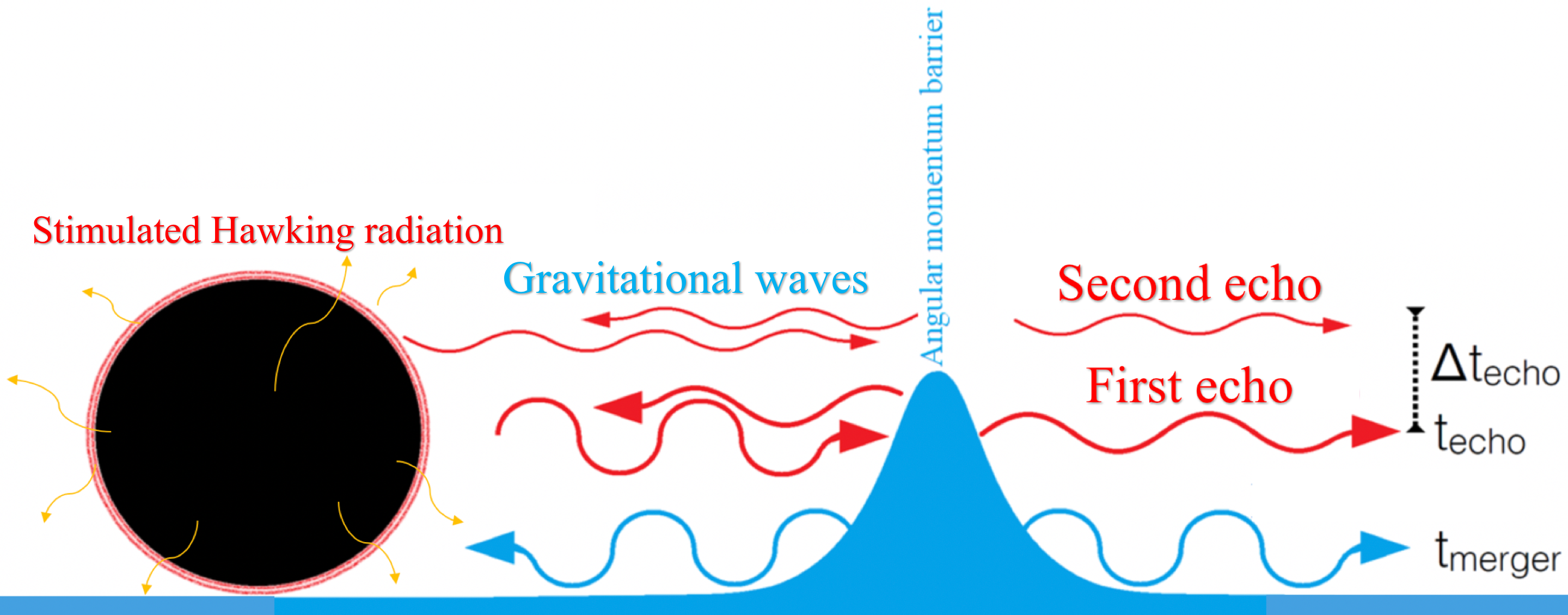
Figure 1: Schematic diagram of GW echoes (stimulated Hawking radiation) from remnant of a BBH merger.

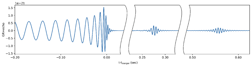
Figure 2: Boltzmann GW echoes template for GW150914 like signal with amplitude $A=1$.

$$\Delta t_{\rm echo}\simeq\frac{4GM_{\rm BH}}{c^{3}}\left(1+\frac{1}{\sqrt{1-a^{2}}}\right)\times\ln\left(\frac{GM_{\rm BH}}{c^{2}\ell_{\rm QG}}\right),$$ (1)

where $M_{\rm BH}$ and $a$ are the mass and the dimensionless spin of the final BH remnant. Here, $\ell_{\rm QG}$ is the characteristic physical length scale for quantum gravity effects where GWs are reflected near the (would-be) horizon. For $\ell_{\rm QG}=\ell_{\rm Planck}$, the reflection happens at a Planck distance from the horizon. More generally, for $\ell_{\rm QG}=\ell_{\rm Planck}/\Lambda$, deviations from GR happen sub-Planckian $\Lambda>1$ or super-Planckian $\Lambda<1$ scales. In this paper, we choose a conservative prior $-13\leq\log_{10}\Lambda\leq 13$.

Here, in comparison to former attempts, I used a more physical waveform, based on stimulated Hawking radiation[34, 35] to test for the existence of echoes. Furthermore, I adopt the Bayesian methodoly and p, as in Abedi et al. [26]. Note that this search has been implemented before the search and release of [26]. The delay in release was due to large number of events and high computational costs to combine all 65 events. In this approach, I set our model and search pipeline from a rather novel point of view to look for echoes combining 65 LVK BBH merger events. I perform the search for echoes on BBH signals using the GWTC-1 [4], GWTC-2 [5] and GWTC-3 [6]. This search includes almost the bulk of all the confident observations [4, 5, 6]. The missed events are either the marginal ones or needed a high computational cost (ones with very small mass). In this approach of combining events I assume echo model is the same for all the events. In particular, I assume all the events have same echo amplitude $A$. Although, this approach does not cover entire space of former searches, it makes a complementary search in overall.

One such proposal to search for quantum black holes in GW data is given by phenomenological Boltzmann echoes waveform [34, 35], where the general relativistic prediction for GW signal from BBH mergers $h_{\rm GR}(\omega)$ in Fourier space is modified to:

$$h_{\rm GR+echoes}(A,\omega)=h_{\rm GR}(\omega)\left[1+Ae^{i\phi}\sum_{n=1}^{\infty}{\cal R}^{n}\right],$$ (2)

$${\cal R}\equiv\exp[-\frac{\hslash|\omega-m\Omega_{H}|}{2kT_{H}}+i\omega\Delta t_{\rm echo}],$$ (3)

where $Ae^{i\phi}$ quantifies their overall amplitude, while the modulus and phase of ${\cal R}$ quantify their relative damping and temporal separation, respectively. Generally, we expect $0\lesssim A\lesssim 2$ and $0<\phi\leq 2\pi$ due to GR non-linearities. Furthermore, I set the horizon mode frequency $m\times\Omega_{H}$ to m=2 for quadrupolar gravitational radiation (with the assumption that the energy in BBH ringdown and echoes are dominated by this mode) as main frequency of search pipeline.

Although, there is no doubt that the $h_{\rm GR}(\omega)$ (main event GR part) exists, we want to answer whether the echoes part exists. Existence of $h_{\rm GR}(\omega)$ helps us to obtain physical prior for echo model i.e. improvements in priors for $\Delta t_{\rm echo}$ in (1) or $\Omega_{H}$ and $T_{H}$ variables. Here, the Boltzmann factor $\exp[-\frac{|\omega-2\Omega_{H}|}{2T_{H}}]$ originates from Hawking tunnelling rate to fuzzy states of quantum BH (please see Fig 2 for this waveform). Note that, repeating echoes time delay modifies this factor to $\exp[\frac{\omega-2\Omega_{H}}{2T_{H}}+i\omega\Delta t_{\rm echo}]$ [34, 35]. Here, I only keep first two echoes of the waveform in this search pipeline. Indeed, this waveform is not as perfect as GR waveform, while it helps us in future research and establishment of better waveforms.

Next section describes method and search pipeline. Then, I conclude with the search results and findings.

2 Method and search pipeline and results

In order to combine the events, the amplitude A for all the 65 events is fixed to a universal value and the individual bayes factors of events B_Event(A) are combine as follows.

$$\rm Combined\ Bayes\ Factor=B(A)=\displaystyle\prod_{i=\rm Events}B_{i}(A)$$ (4)

The combined bayes factors is shown in Figs. 3(a) and 3(b).

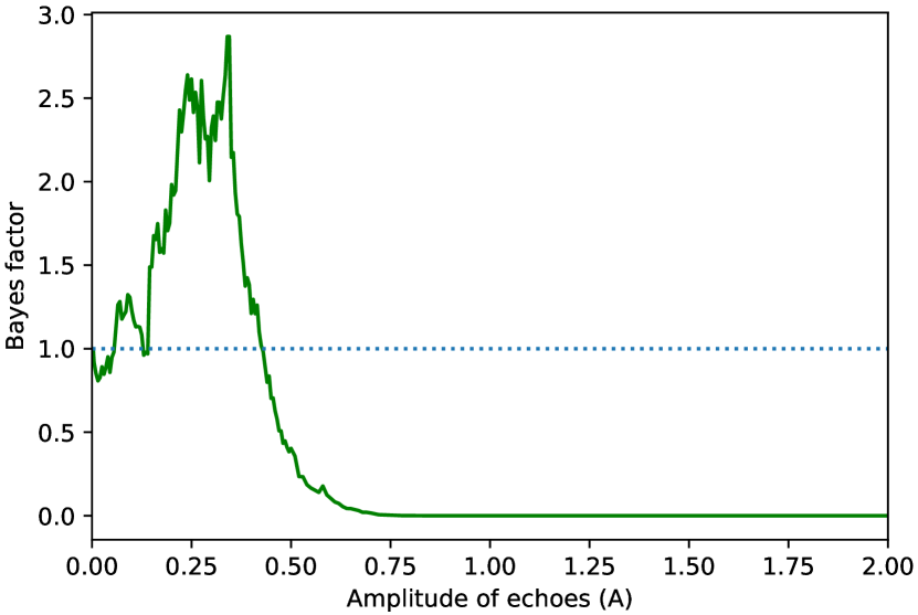
(a)

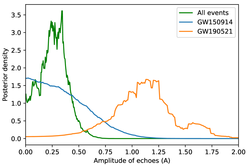
(b)

Figure 3: (a): Combined Bayes factor density in terms of amplitude for 65 events. Combined events give an overall value of $\mathcal{B}^{\rm{GR+echo}}_{\rm{GR}}\simeq 0.4$ for bayes factor. (b): Combined bayes factor posterior density where the bayes factor curves are normalized by $\int_{A_{min}}^{A_{max}}B(A)dA$. Here, in order to compare the individual events (GW150914 and GW190521) and combined events we plot the posterior density of the bayes factors.

I employed PyCBC inference [38] pipeline using a dynamic nested sampling MCMC algorithm, dynesty [39]. It is based on sampling the likelihood function for a hypothesis that gives a measure of existence of a signal in the data. The likelihood function is supposed to be compatible with the natural assumption that the background is Gaussian. I have used two/three detector networks H1-L1/H1-L1-V1 (Hanford, Livingston, Virgo) depending on the event and available data for this analyse. First I obtain the Bayes factor comparing the log likelihood to the log likelihood of the Gaussian noise. Then the combined Bayes factors of alternative models with different amplitude A are compared (here they are $h_{\rm GR+echoes}(A,\omega)$ and $h_{\rm GR+echoes}(A=0,\omega)=h_{\rm GR}(\omega)$ in Eq. (2)). I used class of phenomenological IMR waveform family IMRPhenomPv2 [40, 41] which is freely available as part of LALSuite [42]. Although the main search in Abedi et al. [26] for GW190521 has been performed with NRSur7dq4 waveform [43], in order to make identical search with other events in this paper I employed IMRPhenomPv2 for this event. The slight change in reported bayes factor for this event in this paper is due to change in waveform. It is worth to mention that other waveforms/changes have shown consistent result for this event [26].

For each event I run for discrete set of amplitudes, where each run has different seed number. Since the bayes factor estimation in PyCBC has error, it would be hard to read the result. Due to this error and in order to get smooth/stable result, for each amplitude $A$, the bayes factor density $\bar{B}(A)$ which is the average of $B(A)$ within $(A-\Delta A/2,A+\Delta A/2)$ (see Figs. 3(a) and 3(b)) evaluated. Although the lower $\Delta A$ gives a better resolution, it leads to more fluctuations and error. In order to improve the resolution one needs to increase the number of runs (increase the amplitude bins) as well, which leads to higher computational cost. So it requires a balance between computational cost and targeted resolution. In order to get a satisfying smoothness along with optimum computational cost $\Delta A=0.2$ is chosen. In order to satisfy the approximation, three amplitude range is arranged. First range is near zero $A\sim 0$ which is the place of GR model for comparison. This range needs to have as high as possible runs to estimate the bayes factor of GR accurately. I chose $A=(10^{-4},2\times 10^{-4},3\times 10^{-4},5\times 10^{-4},10^{-3},2\times 10^{-3},3\times 10^{-3},5\times 10^{-3})$ for amplitude bins to accomplish this task. Here the bayes factor is re-normalized to $B(A\sim 0)=1$. The second range is where the combined bayes factor is $B(A)\geq 1$. This range is between $\sim(0,0.5)$ with uniform intervals of $dA=5\times 10^{-3}$. In order to get satisfying result this range needs to have second priority in amplitude resolution. The last range where the bayes factor drops significantly from 1 doesn’t need to have high resolution as it already disfavoured by model when the events are combined. This range is between $(0.5,2)$ with uniform intervals of $dA=0.01$. However, for individual events one may need high resolution in all the amplitudes as well. I set 257 runs for each event and $65\times 257=16705$ runs in total.

In order to obtain the overall bayes factor of individual events and combined events we just do $\mathcal{B}^{\rm{GR+echo}}_{\rm{GR}}=\frac{1}{A_{max}-A_{min}}\int_{A_{min}}^{A_{max}}B(A)dA$ with $(A_{min},A_{max})=(0,2)$. For combined events I got $\mathcal{B}^{\rm{GR+echo}}_{\rm{GR}}\simeq 0.4$. The result for individual events and their histogram are reported in Table 1 and Fig. 4 respectively.

GWTC-1	$\log_{10}\mathcal{B}^{\rm{GR+echo}}_{\rm{GR}}$	GWTC-1	$\log_{10}\mathcal{B}^{\rm{GR+echo}}_{\rm{GR}}$	GWTC-1	$\log_{10}\mathcal{B}^{\rm{GR+echo}}_{\rm{GR}}$
GW150914	-0.53	GW170608	0.05	GW170818	-0.06
GW151012	0.05	GW170729	-0.12	GW170823	-0.25
GW151226	-0.09	GW170809	0.08
GW170104	0.13	GW170814	-0.30
GWTC-2	$\log_{10}\mathcal{B}^{\rm{GR+echo}}_{\rm{GR}}$	GWTC-2	$\log_{10}\mathcal{B}^{\rm{GR+echo}}_{\rm{GR}}$	GWTC-2	$\log_{10}\mathcal{B}^{\rm{GR+echo}}_{\rm{GR}}$
GW$190408\_181802$	-0.16	GW190521	0.96	GW$190728\_064510$	-0.01
GW190412	-0.09	GW$190521\_074359$	-0.54	GW$190731\_140936$	-0.15
GW$190413\_052954$	0.03	GW$190527\_092055$	0.01	GW190814	-0.42
GW$190413\_134308$	-0.10	GW$190602\_175927$	-0.22	GW$190828\_063405$	0.04
GW$190421\_213856$	0.21	GW$190620\_030421$	-0.16	GW$190828\_065509$	-0.14
GW$190424\_180648$	-0.17	GW$190630\_185205$	-0.17	GW$190910\_112807$	-0.30
GW$190503\_185404$	-0.02	GW$190706\_222641$	-0.06	GW$190915\_235702$	-0.09
GW$190512\_180714$	-0.06	GW$190707\_093326$	-0.02	GW$190924\_021846$	0.00
GW$190513\_205428$	-0.15	GW$190708\_232457$	-0.01	GW$190925\_232845$	-0.03
GW$190514\_065416$	-0.03	GW$190719\_215514$	-0.01	GW$190929\_012149$	-0.13
GW$190517\_055101$	0.07	GW$190720\_000836$	-0.07
GW$190519\_153544$	-0.35	GW$190727\_060333$	-0.30
GWTC-3	$\log_{10}\mathcal{B}^{\rm{GR+echo}}_{\rm{GR}}$	GWTC-3	$\log_{10}\mathcal{B}^{\rm{GR+echo}}_{\rm{GR}}$	GWTC-3	$\log_{10}\mathcal{B}^{\rm{GR+echo}}_{\rm{GR}}$
GW$191109\_010717$	-0.36	GW$200112\_155838$	-0.28	GW$200219\_094415$	-0.07
GW$191129\_134029$	0.01	GW$200128\_022011$	-0.2	GW$200220\_061928$	0.21
GW$191204\_171526$	0.01	GW$200129\_065458$	-0.43	GW$200224\_222234$	-0.34
GW$191215\_223052$	0.2	GW$200202\_154313$	0.21	GW$200225\_060421$	-0.01
GW$191216\_213338$	0.03	GW$200208\_130117$	0.08	GW$200302\_015811$	-0.12
GW$191222\_033537$	-0.32	GW$200209\_085452$	0.14	GW$200311\_115853$	-0.37
GW$191230\_180458$	-0.21	GW$200216\_220804$	-0.15	GW$200316\_215756$	-0.01

Table 1: Results of bayes factor for GW echoes in GWTC-1, GWTC-2, and GWTC-3 events. Positive value of the $\log_{10}$ bayes factor indicates a preference for the GR+echoes model over GR model, while the negative value suggests instead a preference for the GR model over the GR+echoes model. Here GW190521 shows loudest echo. Here based on [44] all the individual events appear as inconclusive to both GR or GR+echoes with GW190521 as exception! (see Fig. 4).

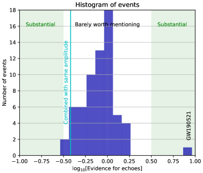
Figure 4: Histogram of $\log_{10}$ bayes factors of 65 events in Table 1. Vertical regions identify Jeffreys scale for interpretation of bayes factor [44].

3 Conclusion and discussions

I presented the outcome which gives measure of possibility for preference of $h_{\rm GR+echoes}$ over $h_{\rm GR}$ based on Bayes factors comparison of these two models. The 65 analysed events in Table 1 and Fig. 4 for individual events show inconclusive result in preference for GR or GR+echo, although with slight preference for GR but not by much. The main scope and result of the paper is combination of echoes for large number of events. We see that the combined bayes factor which is $\mathcal{B}^{\rm{GR+echo}}_{\rm{GR}}$ $\simeq 0.4$ is still inconclusive about GR+echo and GR. It is realised that this combining method gives five order of magnitude higher bayes factor compared to when we simply combine the individual events bayes factor via multiplication $\displaystyle\prod_{i=\rm Events}\displaystyle{\mathcal{B}_{i}}^{\rm{GR+echo}}_{\rm{GR}}=2.2\times 10^{-6}$. In another words the fact that the combined bayes factor for preference to GR has dropped from $\sim 4.6\times 10^{5}$ to $\sim 2.5$ indicates that there are still much to do in method improvement. Additionally, the large number of events and computational costs is a guarantee against bayes factor hack making the result robust. The only event that has shown evidence for preference of GR+echo model is GW190521 with $\mathcal{B}^{\rm{GR+echo}}_{\rm{GR}}=9.2$ (see Fig. 4). This is the most massive and confidently detected BBH merger event observed to date [5]. I refer the detailed interpretation and investigation about this event to Abedi et al. [26]. Presuming a simple speculation that we can compare all the events as same (echo model remain same for all the 65 events and their echo amplitudes compare to main event amplitude doesn’t change by much despite the change in initial condition of the progenitor BBH mergers) and all the 65 BBH events should show evidence for echo signals in this model and the space of parameters considered in this search, I found an upper bound amplitude $A<0.42$ (at 90% confidence level) for echoes. I remind the reader that bounds from our search only relate to the family of echo waveforms considered here.

It is worth to note that I didn’t see any evidence for echoes in O1 in contrast to [11, 16, 17], possibly because the model I used here is different and has much suppressed amplitudes in contrast to ADA model in [11].

In order to do a better search for quieter echoes, we might need to have a more physical echo waveforms. In another words, concrete models from alternatives to GR are needed to use in PyCBC pipeline. Without better models, we might wait for O4. Observations will improve in number. LISA, Einstein Telescope, and Cosmic Explorer will make a big breakthrough in sensitivity in search for alternatives to GR.

References

- [1] V. Cardoso, E. Franzin and P. Pani, Phys. Rev. Lett. 116 (2016) no.17, 171101 [erratum: Phys. Rev. Lett. 117 (2016) no.8, 089902] doi:10.1103/PhysRevLett.116.171101 [arXiv:1602.07309 [gr-qc]].
- [2] V. Cardoso, S. Hopper, C. F. B. Macedo, C. Palenzuela and P. Pani, Phys. Rev. D 94 (2016) no.8, 084031 doi:10.1103/PhysRevD.94.084031 [arXiv:1608.08637 [gr-qc]].
- [3] J. Abedi, N. Afshordi, N. Oshita and Q. Wang, Universe 6 (2020) no.3, 43 doi:10.3390/universe6030043 [arXiv:2001.09553 [gr-qc]].
- [4] B. P. Abbott et al. [LIGO Scientific and Virgo], Phys. Rev. X 9 (2019) no.3, 031040 doi:10.1103/PhysRevX.9.031040 [arXiv:1811.12907 [astro-ph.HE]]. Copy to ClipboardDownload
- [5] R. Abbott et al. [LIGO Scientific and Virgo], Phys. Rev. X 11 (2021), 021053 doi:10.1103/PhysRevX.11.021053 [arXiv:2010.14527 [gr-qc]].
- [6] R. Abbott et al. [LIGO Scientific, VIRGO and KAGRA], [arXiv:2111.03606 [gr-qc]].
- [7] B. P. Abbott et al. [LIGO Scientific and Virgo], Phys. Rev. Lett. 116 (2016) no.6, 061102 doi:10.1103/PhysRevLett.116.061102 [arXiv:1602.03837 [gr-qc]].
- [8] B. P. Abbott et al. [LIGO Scientific and Virgo], Phys. Rev. Lett. 116 (2016) no.22, 221101 [erratum: Phys. Rev. Lett. 121 (2018) no.12, 129902] doi:10.1103/PhysRevLett.116.221101 [arXiv:1602.03841 [gr-qc]].
- [9] B. P. Abbott et al. [LIGO Scientific and VIRGO], Phys. Rev. Lett. 118 (2017) no.22, 221101 [erratum: Phys. Rev. Lett. 121 (2018) no.12, 129901] doi:10.1103/PhysRevLett.118.221101 [arXiv:1706.01812 [gr-qc]]. Copy to ClipboardDownload
- [10] B. P. Abbott et al. [LIGO Scientific and Virgo], Phys. Rev. Lett. 123 (2019) no.1, 011102 doi:10.1103/PhysRevLett.123.011102 [arXiv:1811.00364 [gr-qc]].
- [11] J. Abedi, H. Dykaar and N. Afshordi, Phys. Rev. D 96 (2017) no.8, 082004 doi:10.1103/PhysRevD.96.082004 [arXiv:1612.00266 [gr-qc]].
- [12] R. S. Conklin, B. Holdom and J. Ren, Phys. Rev. D 98 (2018) no.4, 044021 doi:10.1103/PhysRevD.98.044021 [arXiv:1712.06517 [gr-qc]].
- [13] J. Abedi and N. Afshordi, JCAP 11 (2019), 010 doi:10.1088/1475-7516/2019/11/010 [arXiv:1803.10454 [gr-qc]].
- [14] N. Uchikata, H. Nakano, T. Narikawa, N. Sago, H. Tagoshi and T. Tanaka, Phys. Rev. D 100 (2019) no.6, 062006 doi:10.1103/PhysRevD.100.062006 [arXiv:1906.00838 [gr-qc]].
- [15] B. Holdom, Phys. Rev. D 101 (2020) no.6, 064063 doi:10.1103/PhysRevD.101.064063 [arXiv:1909.11801 [gr-qc]].
- [16] J. Westerweck, A. Nielsen, O. Fischer-Birnholtz, M. Cabero, C. Capano, T. Dent, B. Krishnan, G. Meadors and A. H. Nitz, Phys. Rev. D 97 (2018) no.12, 124037 doi:10.1103/PhysRevD.97.124037 [arXiv:1712.09966 [gr-qc]].
- [17] A. B. Nielsen, C. D. Capano, O. Birnholtz and J. Westerweck, Phys. Rev. D 99 (2019) no.10, 104012 doi:10.1103/PhysRevD.99.104012 [arXiv:1811.04904 [gr-qc]].
- [18] F. Salemi, E. Milotti, G. A. Prodi, G. Vedovato, C. Lazzaro, S. Tiwari, S. Vinciguerra, M. Drago and S. Klimenko, Phys. Rev. D 100 (2019) no.4, 042003 doi:10.1103/PhysRevD.100.042003 [arXiv:1905.09260 [gr-qc]].
- [19] R. K. L. Lo, T. G. F. Li and A. J. Weinstein, Phys. Rev. D 99 (2019) no.8, 084052 doi:10.1103/PhysRevD.99.084052 [arXiv:1811.07431 [gr-qc]].
- [20] K. W. Tsang, A. Ghosh, A. Samajdar, K. Chatziioannou, S. Mastrogiovanni, M. Agathos and C. Van Den Broeck, Phys. Rev. D 101 (2020) no.6, 064012 doi:10.1103/PhysRevD.101.064012 [arXiv:1906.11168 [gr-qc]].
- [21] R. Abbott et al. [LIGO Scientific and Virgo], Phys. Rev. D 103 (2021) no.12, 122002 doi:10.1103/PhysRevD.103.122002 [arXiv:2010.14529 [gr-qc]].
- [22] Y. T. Wang and Y. S. Piao, [arXiv:2010.07663 [gr-qc]].
- [23] J. Westerweck, Y. Sherf, C. D. Capano and R. Brustein, [arXiv:2108.08823 [gr-qc]].
- [24] J. Ren and D. Wu, Phys. Rev. D 104 (2021) no.12, 124023 doi:10.1103/PhysRevD.104.124023 [arXiv:2108.01820 [gr-qc]].
- [25] R. Abbott et al. [LIGO Scientific, VIRGO and KAGRA], [arXiv:2112.06861 [gr-qc]].
- [26] J. Abedi, L. F. L. Micchi and N. Afshordi, [arXiv:2201.00047 [gr-qc]].
- [27] G. Ashton, O. Birnholtz, M. Cabero, C. Capano, T. Dent, B. Krishnan, G. D. Meadors, A. B. Nielsen, A. Nitz and J. Westerweck, [arXiv:1612.05625 [gr-qc]].
- [28] J. Abedi, H. Dykaar and N. Afshordi, [arXiv:1701.03485 [gr-qc]].
- [29] J. Abedi, H. Dykaar and N. Afshordi, [arXiv:1803.08565 [gr-qc]].
- [30] J. Abedi and N. Afshordi, [arXiv:2001.00821 [gr-qc]].
- [31] R. Gill, A. Nathanail and L. Rezzolla, Astrophys. J. 876 (2019) no.2, 139 doi:10.3847/1538-4357/ab16da [arXiv:1901.04138 [astro-ph.HE]].
- [32] Q. Wang and N. Afshordi, Phys. Rev. D 97 (2018) no.12, 124044 doi:10.1103/PhysRevD.97.124044 [arXiv:1803.02845 [gr-qc]].
- [33] J. Abedi, [arXiv:2209.07363 [hep-th]].
- [34] N. Oshita, Q. Wang and N. Afshordi, JCAP 04 (2020), 016 doi:10.1088/1475-7516/2020/04/016 [arXiv:1905.00464 [hep-th]].
- [35] Q. Wang, N. Oshita and N. Afshordi, Phys. Rev. D 101 (2020) no.2, 024031 doi:10.1103/PhysRevD.101.024031 [arXiv:1905.00446 [gr-qc]].
- [36] S. Xin, B. Chen, R. K. L. Lo, L. Sun, W. B. Han, X. Zhong, M. Srivastava, S. Ma, Q. Wang and Y. Chen, Phys. Rev. D 104 (2021) no.10, 104005 doi:10.1103/PhysRevD.104.104005 [arXiv:2105.12313 [gr-qc]].
- [37] M. Srivastava and Y. Chen, Phys. Rev. D 104 (2021) no.10, 104006 doi:10.1103/PhysRevD.104.104006 [arXiv:2108.01329 [gr-qc]].
- [38] C. M. Biwer, C. D. Capano, S. De, M. Cabero, D. A. Brown, A. H. Nitz and V. Raymond, Publ. Astron. Soc. Pac. 131 (2019) no.996, 024503 doi:10.1088/1538-3873/aaef0b [arXiv:1807.10312 [astro-ph.IM]].
- [39] Speagle, J. S. 2020. DYNESTY: a dynamic nested sampling package for estimating Bayesian posteriors and evidences. Monthly Notices of the Royal Astronomical Society 493, 3132–3158. doi:10.1093/mnras/staa278
- [40] S. Khan, S. Husa, M. Hannam, F. Ohme, M. Pürrer, X. Jiménez Forteza and A. Bohé, Phys. Rev. D 93 (2016) no.4, 044007 doi:10.1103/PhysRevD.93.044007 [arXiv:1508.07253 [gr-qc]].
- [41] M. Hannam, P. Schmidt, A. Bohé, L. Haegel, S. Husa, F. Ohme, G. Pratten and M. Pürrer, Phys. Rev. Lett. 113 (2014) no.15, 151101 doi:10.1103/PhysRevLett.113.151101 [arXiv:1308.3271 [gr-qc]].
- [42] LIGO Scientific Collaboration, free software (GPL) doi:10.7935/GT1W-FZ16
- [43] V. Varma, S. E. Field, M. A. Scheel, J. Blackman, D. Gerosa, L. C. Stein, L. E. Kidder and H. P. Pfeiffer, Phys. Rev. Research. 1 (2019), 033015 doi:10.1103/PhysRevResearch.1.033015 [arXiv:1905.09300 [gr-qc]].
- [44] Robert E. Kass and Adrian E. Raftery, Journal of the American Statistical Association, vol. 90, no. 430, 1995, pp. 773–795. JSTOR, https://doi.org/10.2307/2291091.
Acknowledgements
I would like to thank Niayesh Afshordi and Alex B. Nielsen for helpful comments and discussions. I also thank Conner Dailey for suggestion about Fig. 2. I thank the Max Planck Gesellschaft and the Atlas cluster computing team at AEI Hannover for support and computational help. I was supported by ROMFORSK grant Project. No. 302640. This research has made use of data, software and/or web tools obtained from the Gravitational Wave Open Science Center (https://www.gw- openscience.org), a service of LIGO Laboratory, the LIGO Scientific Collaboration and the Virgo Collaboration. LIGO is funded by the U.S. National Science Foundation. Virgo is funded by the French Centre National de Recherche Scientifique (CNRS), the Italian Instituto Nazionale della Fisica Nucleare (INFN) and the Dutch Nikhef, with contributions by Polish and Hungarian institutes.