Bubble in the Whale: Identifying the Optical Counterparts and Extended Nebula for the Ultraluminous X-ray Sources in NGC 4631

Abstract

We present a deep optical imaging campaign on the starburst galaxy NGC 4631 with CFHT/MegaCam. By supplementing the HST/ACS and Chandra/ACIS archival data, we search for the optical counterpart candidates of the five brightest X-ray sources in this galaxy, four of which are identified as ultraluminous X-ray sources (ULXs). The stellar environments of the X-ray sources are analyzed using the extinction-corrected color-magnitude diagrams and the isochrone models. We discover a highly asymmetric bubble nebula around X4 which exhibits different morphology in the H$\alpha$ and [O iii] images. The [O iii]/H$\alpha$ ratio map shows that the H$\alpha$-bright bubble may be formed mainly via the shock ionization by the one-sided jet/outflow, while the more compact [O iii] structure is photoionized by the ULX. We constrain the bubble expansion velocity and interstellar medium density with the MAPPINGS V code, and hence estimate the mechanical power injected to the bubble as $P_{w}\sim 5\times 10^{40}$ erg s^-1 and the corresponding bubble age of $\sim 7\times 10^{5}$ yr. Relativistic jets are needed to provide such level of mechanical power with a mass-loss rate of $\sim 10^{-7}\ M_{\odot}\ \rm yr^{-1}$. Besides the accretion, the black hole spin is likely an additional energy source for the super-Eddington jet power.

1 Introduction

Ultraluminous X-ray sources (ULXs) are non-nuclear point-like X-ray sources with isotropic luminosity $L_{X}\ \gtrsim\ 10^{39}\ \rm erg\ s^{-1}$, which corresponds to the Eddington limit for a $\sim 10\ M_{\odot}$ black hole (Feng & Soria, 2011; Kaaret et al., 2017). Two mechanisms are likely to explain the high luminosity: the sub-Eddington accretion onto intermediate-mass black holes (IMBHs) and stellar-mass compact objects undergoing super-Eddington accretion. The minority of ULXs at the higher end of the luminosity range can be explained by the first mechanism, such as ESO 243$-$49 HLX-1 with $L_{X}\sim 10^{42}~{}\rm erg~{}s^{-1}$ (Farrell et al., 2009; Webb et al., 2012). Meanwhile, the X-ray spectral properties of most ULXs are consistent with the super-Eddington accretion scenario (e.g., Gladstone et al., 2009; Walton et al., 2014; Salvaggio et al., 2022). Recent studies further identified several ULXs powered by neutron stars from the detections of pulsating radiations (Bachetti et al., 2014; Fürst et al., 2016; Israel et al., 2017a, b; Weng et al., 2017; Carpano et al., 2018; Wilson-Hodge et al., 2018; Sathyaprakash et al., 2019; Rodríguez Castillo et al., 2020; Quintin et al., 2021).

The definitive approach to decipher the nature of non-pulsating ULXs is the dynamical mass measurement of the accretors, which relies on the optical spectroscopy of the donor stars. However, the archived optical data on ULXs are far less abundant than X-ray data because most of the ULX optical counterparts are very faint ($m_{V}>21\ \rm mag$) and located in fairly crowded regions. Previous studies found that most of the ULXs are associated with young star clusters, showing the donor stars might be the OB type (Roberts et al., 2008; Poutanen et al., 2013). For a limited number of ULXs, the nature of the donor stars are unambiguously identified (e.g., M101 ULX-1 and NGC 7793 P13), while the dynamical studies on these systems supported the stellar-mass accretor scenario (Liu et al., 2013; Motch et al., 2014).

A number of ULXs have surrounding bubble nebulae detected from deep optical imaging observations (e.g., Pakull & Mirioni, 2002; Ramsey et al., 2006; Soria et al., 2010, 2021), the majority of which are considered to be formed via shock ionizations driven by the interactions of strong jets/outflows and the ambient interstellar medium (ISM). Strong outflows may be ubiquitous for ULXs under supercritical accretion (e.g., Narayan et al., 2017; Weng & Feng, 2018; Zhou et al., 2019; Qiu & Feng, 2021; Kosec et al., 2021). The kinetic power and age of the bubble can be inferred from its size and expanding velocity (Weaver et al., 1977), and hence may reveal the kinematics of jets/outflows and the accretion physics of ULXs (Pakull et al., 2010; Cseh et al., 2012; Soria et al., 2021). For the other few cases, the high-ionization features (e.g., He ii $\lambda 4686$) in the spectra of the optical nebulae imply that the photoionization could be the major origin of the extended structure (Pakull & Mirioni, 2002). Both shock ionization and photoionization may certainly be working at the same time while dominating different parts of the same optical nebula (Gúrpide et al., 2022; Zhou et al., 2022).

In this work, we report on an optical broad-band and narrow-band imaging campaign for the Whale Galaxy NGC 4631 to identify the optical counterparts and surrounding extended nebulae of the ULXs, for which Soria & Ghosh (2009) presented a detailed study of their X-ray properties. As a late-type starburst galaxy 7.35 Mpc away, NGC 4631 (Figure 1) has been extensively studied in multiwavelengths. The existence of molecular outflows, abundant gas and the X-ray halo reveals the diversity of objects and astrophysical processes (e.g., Yamasaki et al., 2009; Irwin et al., 2011; Meléndez et al., 2015). From the archival XMM-Newton data, Soria & Ghosh (2009) identified five brightest X-ray sources scattered in NGC 4631 and found that four of them (X1, X2, X4, X5) can be classified as ULXs. For the purpose of studying their physical nature and stellar environments, we analyze the optical images of all five X-ray sources in this paper combining the Canada-France-Hawaii Telescope (CFHT) and Hubble Space Telescope (HST) observations, supplemented with Chandra data to determine the precise astrometry. The details of the five X-ray sources can be found in Table 1.

This paper is organized as follows. In Section 2 we present the optical and X-ray observations and data reduction. In Section 3, we improve the relative astrometry and identify optical counterpart candidates for the X-ray sources, which are investigated in Section 4 based on their locations on the isochrone diagrams. In Section 5, we present a newly discovered bubble nebula around X4 and the analyses on its morphology and kinetic power. Section 6 summarizes our conclusions.

Table 1: List of the Five Brightest X-ray Sources in NGC 4631

Source ID	R.A.	Dec.	Chandra Net Counts	Off-axis	Opt-X Error Circle	$N_{\rm H}$	E(F606W-F814W)
	(J2000)	(J2000)	(0.5–8.0 keV)	(arcmin)	(arcsecond)	($10^{21}$ cm-2)
X1	12 42 15.99	+32 32 49.47	6.7$\pm{2.8}$	4.10	0.673	2.4${}^{+0.3}_{-0.3}$	0.35${}^{+0.15}_{-0.15}$
X2	12 42 11.12	+32 32 35.63	981.2$\pm{32.9}$	3.05	0.275	28.3${}^{+3.6}_{-3.2}$	3.80${}^{+1.74}_{-1.55}$
X3	12 42 06.13	+32 32 46.43	357.6$\pm{19.6}$	2.11	0.269	2.0${}^{+1.0}_{-0.9}$	0.29${}^{+0.48}_{-0.43}$
X4	12 41 57.42	+32 32 02.79	77.7$\pm{9.2}$	0.19	0.280	0.32${}^{+1.02}_{-0.32}$	0.05${}^{+0.49}_{-0.16}$
X5	12 41 55.57	+32 32 16.77	2977.8$\pm{55.8}$	0.51	0.268	2.0${}^{+0.2}_{-0.2}$	0.29${}^{+0.10}_{-0.10}$

Note. — The $N_{\rm H}$ values are retrieved from Soria & Ghosh (2009) which were obtained from the Chandra spectral analyses.

Table 2: Observation Log of NGC 4631

Instrument		Source ID		ObsID		Filter		Observation Date (UT)		Exposure Time
CFHT/MegaCam		X1-X5		20AS01		H$\alpha$		2020-03-23		12$\times$900 sec
(PI: Jing Guo)						[O iii]		2020-05-19		5$\times$750 sec
						$u$		2020-03-23		5$\times$126 sec
						$g$		2020-03-23		5$\times$126 sec
						$r$		2020-03-23		5$\times$126 sec
HST/ACS		X1,X2,X3		j8r331010		F606W		2003-08-03		676 sec
		X1,X2,X3		j8r331020		F814W		2003-08-03		700 sec
		X4, X5		j8r332010		F606W		2004-06-09		676 sec
		X4, X5		j8r332020		F814W		2004-06-09		700 sec
Chandra/ACIS		X1-X5		797				2000-04-16		60 ksec

Table 3: List of the reference stars

Reference ID	X-ray Coordinates	Optical Coordinates	Off-axis	Net Counts	X-ray positional error
	Chandra	HST	(arcmin)	Chandra	(arcsecond)
Ref.1	12 42 25.78 +32 33 21.40	12 42 25.79 +32 33 21.23	6.2	$120\pm 11$	0.32
Ref.2	12 42 04.03 +32 34 08.60	12 42 04.03 +32 34 08.41	2.7	$107\pm 10$	0.19

Note. — The HST coordinates are given by the Dolphot package.

2 Observations and Data reduction

2.1 CFHT

We obtained optical broad-band and narrow-band imaging of NGC 4631 with the 3.6-m CFHT located on Mauna Kea, Hawaii. The MegaCam instrument mounted on CFHT has a wide field of view (1 deg²) which can fully cover all the 5 luminous X-ray sources in NGC 4631. The detector consists of 40 CCDs, each of which has $2048\times 4612$ pixels with $0\farcs 187\times 0\farcs 187$ per pixel. We are awarded a total of 4.5-hour exposure time (PI: Jing Guo, ObsId: 20AS01) executed in 2020 March and June. The images are taken with three broad bands ($u$, $g$, and $r$) and two narrow bands (H$\alpha$ and [O iii]). The H$\alpha$ and [O iii] filters have a width of $\sim 100$ Å, centered at 6590 Å and 5006 Å, respectively. A dithering pattern was applied during the observations to cover the CCD gaps, which requires at least five exposures for each band. The detailed observation log is listed in Table 2.

The data products we received have been preprocessed with the Elixir pipeline, which includes bias-subtraction, flat-fielding, etc., for each individual frame (Magnier & Cuillandre, 2004). The first step is to perform precise astrometric calibration and to stack images from individual exposures in the same band for the purposes of eliminating CCD gaps and reaching the desired sensitivity level. In the stacking procedure, SExtractor (Bertin & Arnouts, 1996) was applied on each image of single exposures to generate the catalog of all point sources with coordinates. The astrometric solutions were then computed with the SCAMP (Bertin, 2006) software by referencing the catalog from Gaia Data Release 1 (DR1). We utilized the SWarp (Bertin, 2010) task to perform the image stacking. The astrometric error during these processes are $<0\farcs 03$. A multi-color image of NGC 4631 is shown in Figure 1. This RGB-like image combines the three broad bands and two narrow bands. The five red circles label the positions of the five luminous X-ray sources analyzed in Soria & Ghosh (2009). X3 is more likely a black hole X-ray binary in its high/soft state, while the remaining four X-ray sources are classified as ULXs, among which X1 is a supersoft ULX.

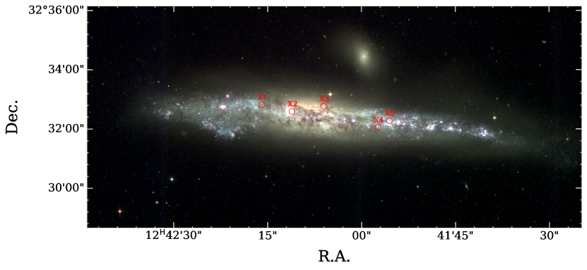
Figure 1: The RGB-like image combines five CFHT/MegaCam filters, including the three broad bands ($u$, $g$, $r$) and two narrow bands (H$\alpha$, [O iii]). The $u$, $g$, and $r$ bands are shown in blue, green, and red colors, respectively, while the H$\alpha$ and [O iii] filters are represented by crimson and teal colors, respectively. The red circles label the positions of the five X-ray sources.

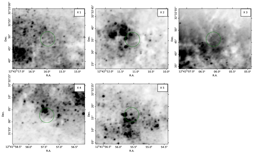
Figure 2: The CFHT/MegaCam $g$-band images of X1-X5 and their vicinity, respectively. The green circles are centered at the X-ray location of each source with a radius of $3\arcsec$. Optical counterparts are difficult to identify in these broad-band images due to the seeing limit ($0\farcs 45$–$0\farcs 75$) for the ground-based CFHT.

We select 40 point sources from the Pan-STARRS1 DR2 catalog (Flewelling, 2018; Flewelling et al., 2020) that are isolated and have an appropriate magnitude (17–19 mag) to serve as photometry references. The Pan-STARRS1 DR2 catalog does not flag the source whether it is a star. Thus we select such a relatively large set of referencing sources aiming to obtain a more statistically reliable photometry calibration. We adopt the conversion equations from Pan-STARRS filters to MegaCam filters provided by the Canadian Astronomy Data Centre (CADC), except for H$\alpha$ we use the formula provided by Boselli et al. (2018). Finally, for each given source, we can derive an array of magnitude values calibrated from the 40 reference stars. The peak value of the best-fit Gaussian profile to the histogram of the magnitude values was adopted as the measured magnitude for this source.

The zoom-in CFHT/MegaCam $g$-band images of the five luminous X-ray sources are shown in Figure 2. For the stacked image in each band, we estimate the exposure depth reaching 25–26 mag arcsec^-2 at $3\sigma$ level. Due to the seeing limit of ground-based imaging, it is difficult to identify the exact optical counterparts to the X-ray sources at their crowded locations in the edge-on galaxy NGC 4631. However, in the H$\alpha$ narrow-band images we discover a bubble-like extended nebula surrounding X4, which may be inflated by the jet or wind launched from the ULX accretion disk (Figure 3). The projected size of this bubble structure is $\sim 130$ pc $\times$ 100 pc.

To obtain a more precise profile of the extended bubble structure, we need to subtract the continuum contribution from the H$\alpha$ image. Boselli et al. (2018) utilized a large set of unsaturated stars and derived an empirical equation (see their Eqn. 4) to relate the $g-r$ color and the H$\alpha$ magnitude. Following Boselli et al. (2018), we use the data products which were processed by CADC with MegaPipe upon our request. MegaPipe will subtract the sky background, normalize the flux in the whole stacked image, and provide a catalog of detected point sources (Gwyn, 2008). We filtered out the pixels with low signal-to-noise ratio ($S/N\leqslant 5$), and then applied the equation in Boselli et al. (2018) pixel by pixel. The generated image is shown in the upper right panel of Figure 3. Most of the point sources around X4 have been removed from the H$\alpha$ image. The morphology of the extended structure are clearly revealed.

For the [O iii] narrow-band image, we derived a similar equation connecting the g-r color and the [O iii] magnitude by roughly assuming the continuum magnitude is linearly related to wavelength in the given range (i.e., the continuum follows a power-law spectral profile; see details in Appendix A):

$$m_{g/\rm[O~{}{\sc III}]}\ \approx\ m_{g}-0.155\times(m_{g}-m_{r}),$$ (1)

where $m_{g/\rm[O~{}{\sc III}]}$ is the magnitude of the continuum that falls within the [O iii] narrow-band filter. After applying the equation pixel by pixel, we obtain an [O iii] narrow-band image for which most of the continuum contribution has been eliminated (see the lower right panel of Figure 3). As for the continuum-subtracted H$\alpha$ image, the point sources have been mostly removed from the [O iii] image, proving the efficacy of our continuum subtraction method. We will discuss this bubble structure in details in Section 5.

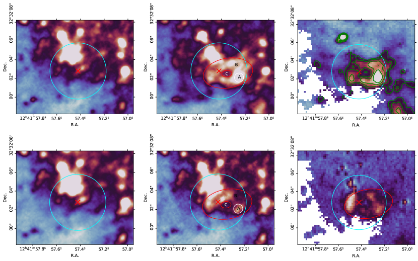
Figure 3: From left to right in the first row, the first panel is the CFHT/MegaCam $r$-band image, where the cyan circle is centered at the X-ray location (the red cross symbol) of X4 with a $3\arcsec$ radius. The half length of the red cross represents the X-ray positional error of X4. The second is the H$\alpha$ image, residing with a bubble-like structure around X4. The brightest region is marked as A region in the white circle. When performing the photometry for the whole bubble, the shape is adopted as the region between the two red ellipses, marked as B (which includes the A region). The cavity in the center is marked as C. The third panel is the result of subtracting the underlying continuum component from the H$\alpha$ image. Most of the stellar sources have been removed here. The blank regions represent the dropped pixels that do not have adequate $S/N$. In the second row, the images of $g$, [O iii] and [O iii] with continuum removed are shown in turn.

2.2 HST

NGC 4631 has been observed with the Advanced Camera for Surveys (ACS; Ford et al. 1998) onboard HST (see Table 2). The five luminous X-ray sources were completely covered by the observations in Proposal 9765. The field containing X1, X2, and X3 was observed in 2003 August (ObsID j8r331010 for the F606W filter and j8r331020 for F814W), while X4 and X5 were covered by the observations in 2004 June (ObsID j8r332010 for F606W and j8r332020 for F814W). Each observation has a total exposure time of 1376 sec. The images of the five X-ray sources in the F606W band are shown in Figure 4.

We aim to identify the optical counterparts of X-ray sources with the HST imaging and derive their magnitudes. Astrometric calibration is also needed for the HST images. As the lack of coverage upon the galaxy disk of NGC 4631 in Gaia, we are not able to directly align HST images with the Gaia references. CFHT images with a large field of view are reused as the reference images to align the HST data. We selected seven reference sources in each HST observation to perform astrometric calibration, for which we obtained the RMS residual of $0\farcs 03$. Then we employed the Dolphot package to perform Point Spread Function (PSF) photometry. Dolphot can identify point sources in heavily crowded areas and return their Vega magnitudes (Dolphin, 2000). The acsmask task was used to flag bad pixels, and the calcsky task can calculate the sky background. After these preprocessing, the PSF photometry was accomplished by the dolphot task. The parameters in dolphot are configured referring to Williams et al. (2014) where they made a series of artificial stars to test a mesh grid parameters and found out the most suitable parameter set for crowded fields.

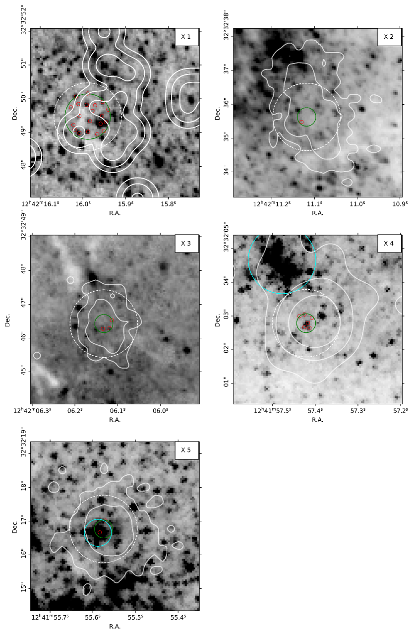
Figure 4: The HST/ACS F606W images of each X-ray source, with the overlaid white contours representing the X-ray flux level from the Chandra/ACIS data (contours not in uniform scales among the five panels). In each panel, the green circle is centered at the X-ray location with the radius represents the respective error circle. The numbered red circles are the optical counterpart candidates of the X-ray source. The white dashed circle has a radius of $1\arcsec$. The cyan circle in the middle right panel marks the young star associations northeast to X4, while that in the bottom left panel labels the compact young star group associated with X5.

2.3 Chandra

In the X-ray band, NGC 4631 has been observed by Einstein, ROSAT, Chandra, and XMM-Newton. To obtain precise locations of the X-ray sources, we reprocessed the Chandra/ACIS data which have a sub-arcsec angular resolution. The Chandra observation (ObsID 797) was carried out on 2000 April 16 for a total of 60 ksec exposure time. We perform X-ray astrometry and photometry in this work. The spectral and timing properties of these X-ray sources were presented in details in Soria & Ghosh (2009).

The data were reprocessed with the CIAO (v4.13) package. The chandra_repro task was applied to create a new $level=2$ event file calling the latest calibration products (CALDB v4.9.4) and more advanced algorithms. For astrometric calibration, we aligned the Chandra/ACIS images to the HST/ACS images (see Section 3 for details).

The CIAO script deflare was used to remove the background flares ($>3\sigma$) which only accounts for $\approx 4\%$ of the total exposure time. The full-band (0.5–8.0 keV) X-ray image was then generated using the ASCA grade 0,2,3,4,6 events. The PSF and exposure maps were produced accordingly. The final X-ray point source detection was carried out using wavdetect. The detection threshold is set to be $10^{-6}$, while the wavelet scales are 1, $\sqrt{2}$, 2, $2\sqrt{2}$, and 4 pixels. The coordinates return by wavdetect are adopted as the X-ray positions for the five luminous X-ray sources.

3 Identifying the optical counterparts

To identify the optical counterparts of the X-ray sources, we improve the astrometry of Chandra/ACIS images relative to the HST/ACS images following the methodology laid out in Yang et al. (2011). Because of the small field of view of HST/ACS, only one common source can be registered from the Chandra to the HST images. Therefore, we supplement the HST/ACS observation on an adjacent and partly overlapping field (ObsID jc9l04010) to taking a mosaic image using the AstroDrizzle package. The second common source is therefore added. These two objects are identified as point X-ray sources (Wang et al., 2016; Evans et al., 2010), and their coordinates and other information are listed in Table 3. We use the CIAO task wcs_match to register the Chandra image to the HST image. The RMS residual is $0\farcs 02$. The updated positions of five X-ray sources are listed in Table 1.

We calculated the 95% Chandra positional error radius for each source using Equation 5 in Hong et al. (2005) which has considered the PSF variations across the field of view. We then converted it to the 1$\sigma$ error radius by applying the relation $r_{X}=r_{X(95\%)}/1.95996$ in Zhao et al. (2005). The size of the error circle is primarily related to the number of counts and the off-axis angle of the source. Finally, we adopt the positional uncertainty of each source as the quadratical combination of all kinds of errors: the average X-ray positional error of the two reference objects ($0\farcs 19$), the X-ray positional error of each X-ray source ($0\farcs 15$-$0\farcs 63$), the error caused by the alignment between the HST and Chandra images, and the error of optical coordinates which were generated during the astrometric calibration of HST and CFHT images. The latter two kinds of errors are both ignorable compared to the X-ray positional errors. The final positional uncertainties of the five X-ray sources are listed in Table 1.

In Figure 4, we overlay the X-ray flux contours (solid white lines) onto the HST/ACS/F606W images for each X-ray source. The green circles represent the uncertainties of X-ray positions. X1 has the largest error circle ($0\farcs 66$) because of the small number of Chandra net counts ($\approx 7$). There are multiple candidate optical counterparts for X1 detected by Dolphot, which are labeled by small red circles in the upper left panel of Figure 4. The error radii of X2–X5 are similar ($\sim 0\farcs 3$). X2 has one candidate optical counterpart in its X-ray positional error circle, while both X3 and X4 have a few candidates in their respective error circles. X5 is located within a crowded region while two individual sources are detected in the error circle. We will analyze these candidate optical counterparts and the surrounding stellar environments in the next section.

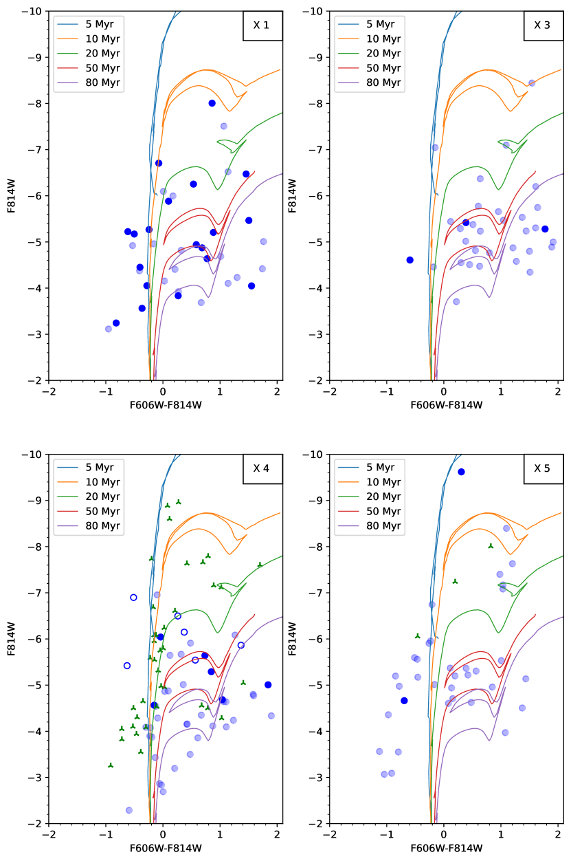
Figure 5: The color-magnitude diagrams (CMDs) for optical point sources around X1, X3, X4, and X5, respectively. The solid blue dots are the optical counterpart candidates within the error circle. The light blue dots are the point sources within $1\arcsec$ but outside the error circle which could be born in the same environment. The green $tri\_up$ symbols in left-lower panel represent the sources in the star group northeast of X4. Extinction correction has been applied based on the X-ray hydrogen column density. The open blue circles labels the loci of the optical counterpart candidates of X4 when the extinction value is adopted from the XMM-Newton spectral modeling.

4 Color-Magnitude Diagram

For most ULXs, the optical emission is dominated by the X-ray reprocessing on the accretion disk (Tao et al., 2011). Nevertheless, the optical Color-Magnitude Diagrams (CMD) can be used to infer the age of the stellar environments around ULXs, which could potentially suggest the nature of the ULX donor stars. The Padova Stellar Evolution Code (PARSEC; Bressan et al. 2012) provides the isochrone databases for almost all the mainstream telescope filters. Here we utilize the isochrones based on the HST/ACS filters system.

We derive the extinction $A_{V}$ from the hydrogen column density obtained by Soria & Ghosh (2009) via X-ray spectral analyses of the Chandra observations based on the relation of $N_{\rm H}$ (cm^-2) $=(2.21\pm 0.09)\times 10^{21}$ $A_{V}$ (mag) presented in Güver & Özel (2009). To convert $A_{V}$ to the extinction in the HST/ACS filter system $E{\rm(F606W-F814W)}$, we then interpolate the central wavelengths of these filters to the extinction law derived in Cardelli et al. (1989). The extinction value for each X-ray source is listed in Table 1.

Closely aligned with a young stellar cluster, X2 has large extinction $E{\rm(F606W-F814W)}=3.8$ mag, which may introduce significant uncertainties when applying the CMD to derive the ages of its surrounding stars. Therefore, we only plot the isochrones for the other four X-ray sources (Figure 5). For each panel, the solid blue dots stand for the optical counterpart candidates of the X-ray source. The light blue dots represent the stars within $1\arcsec$ (36 pc; see the white dashed circles in Figure 4) from the X-ray position but outside the optical-to-X-ray error circle.

The immediate surrounding stars of X1 do not appear to be closely associated like in a star group or cluster. Its optical counterpart candidates, as well as the nearby stars within $1\arcsec$, span a wide range of age from 5 Myr to 80 Myr, which indicates that they are unlikely born at the same time or in the same environment. As discussed in Section 3, the positional error circle of X1 is also much larger ($0\farcs 673$), corresponding to $\approx 25$ pc. For X2, the sole optical counterpart shown in Fig 4 is likely to be not reliable because of the large extinction. For X3, the three optical counterpart candidates have ages of $\sim$50–80 Myr which are consistent with the ages of the environmental sources. For X4, the ages of the surrounding stars range mostly in $\sim 20$–80 Myr. The six candidate optical counterparts also show similar ages. There appears to be a star association northeast of X4 with the size of $\approx 2\arcsec$ across (71 pc). The CMD shows that most of its member stars are very young with ages of 5–20 Myr (the green $tri\_up$ symbols in the lower left panel of Figure 5). It is worth noting that the $N_{\rm H}$ value of X4 derived from the XMM-Newton spectral modeling is one order of magnitude higher than that with the Chandra data (Soria & Ghosh, 2009). The optical counterpart candidates of X4 would be younger, $<$ 20 Myr (see fig 5), if the XMM-Newton extinction value were adopted. X5 appears to locate within a compact star group ($\approx 0\farcs 8$ across; corresponding to 28 pc). Two point sources are identified within the error circle with ages of $\sim$ 5 Myr, while three more individual sources in this star group are resolved by Dolphot, which have ages $\sim 5$–10 Myr (the green $tri\_up$ symbols in Figure 5 lower right panel). Therefore, X5 is likely associated with a young star cluster.

It is worth noting that the extinction derived from the hydrogen column density obtained with X-ray spectra represent an upper limit for the candidate optical counterparts and their surrounding stars. If significant intrinsic absorption exists for the X-ray source, the extinction would be much smaller. A conservative lower limit would be the Galactic extinction along the light of sight of NGC 4631, which is $A_{V}=0.015$ mag (Schlafly & Finkbeiner, 2011), corresponding to $N_{\rm H}=3.3\times 10^{19}$ cm^-2. This is ignorable compared to that from the X-ray spectroscopy. The true values of extinction should be in between the above lower and upper limits. Overestimation of the extinction would place the stars at younger age regions on the CMD. However, it is probably reasonable to assume that the candidate optical counterparts and surrounding stars would suffer from high extinction (i.e., close to the upper limits), since NGC 4631 appears as an edge-on disk galaxy.

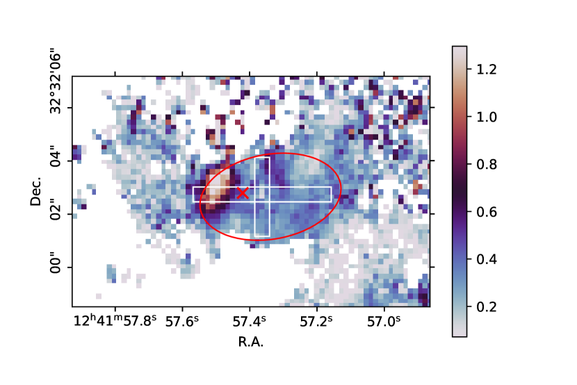
Figure 6: The [O iii]/H$\alpha$ flux ratio map for the extended structure around X4, where the vertical color bar shows the line ratio values. The red ellipse represents the profile of the H$\alpha$ bubble, while the red cross marks the position of X4. The white horizontal and vertical bars illustrate the major and minor axes of the extended structure.

5 A Newly Discovered Bubble Structure Around X4

5.1 Morphology Analysis

Both of the continuum-subtracted H$\alpha$ and [O iii] images display a clear extended structure around X4 (see the right two panels in Figure 3), while exhibiting different morphology in the two bands. In the H$\alpha$ image, the structure appears more like an inflated bubble with the size of $\sim 130$ pc $\times$ 100 pc. The X-ray source X4 is not located in the center. Instead, this H$\alpha$ bubble structure appears to be sourced from the location of the ULX (see the red cross in Figure 3) and is oriented toward the southwest direction, reaching maximum luminosity in the outermost region, $\sim 100$ pc away from X4. The extended nebula in the [O iii] image has a smaller size. In contrast to the H$\alpha$ bubble, the brightest region of the [O iii] structure is to the east of X4, and is substantially closer to the X-ray source ($\lower 2.0pt\hbox{$\,\buildrel\scriptstyle<\over{\scriptstyle\sim}\,$}25$ pc).

The extended structures around ULXs may originate from photoionization or shock ionization, both of which could coexist while playing major roles in different parts of the structure (Moon et al., 2011; Gúrpide et al., 2022; Zhou et al., 2022). Generally, in the photoionization process, the line flux ratio [O iii]/H$\beta$ tends to peak at or near the ionizing source and declines outwards. For the shock-ionized bubble, the edge region has higher excitation level and exhibits the higher [O iii]/H$\beta$ ratio than in the central area. Here we use the [O iii]/H$\alpha$ ratio as a proxy, since it is reasonable to assume that the line ratio $H\alpha/H\beta\equiv\tau$ remains constant in the bubble area. The typical $\tau$ value is $\sim 3$ for ULX bubbles (Allen et al., 2008). We will calculate the exact value for our case in the next subsection. Derived from the continuum-subtracted [O iii] and H$\alpha$ images, the [O iii]/H$\alpha$ ratio map is shown in Figure 6, in which the red ellipse marks the bubble shape in the H$\alpha$ band (same as that in the upper middle panel of Figure 3). We extract the [O iii]/H$\alpha$ line ratio roughly along the major and minor axes of the bubble (the white horizontal and vertical bars in Figure 6 respectively) and obtain a clearer spatial profile, which is illustrated in Figure 7. The [O iii]/H$\alpha$ ratio reaches its minimum in the bubble center and increases outwards along both axes, which suggests that the H$\alpha$ bubble is mostly dominated by the shock ionization. There is a bump of the [O iii]/H$\alpha$ ratio in the east edge of major axis, coinciding with the brightest [O iii] region. This area is likely formed predominantly by photoionization. It is indeed close to the ULX which is presumably the source of ionizing photons. The peak [O iii]/H$\alpha$ value in this area is $\lower 2.0pt\hbox{$\,\buildrel\scriptstyle>\over{\scriptstyle\sim}\,$}1$. Combined with the calculated $H\alpha/H\beta$ line ratio of $\tau\sim 3.75$ (see Section 5.2), the peak [O iii]/H$\beta$ would be $\sim 4$, which is similar to that of photoionization-dominated nebulae found in previous ULX bubble studies (e.g., Soria et al. 2021).

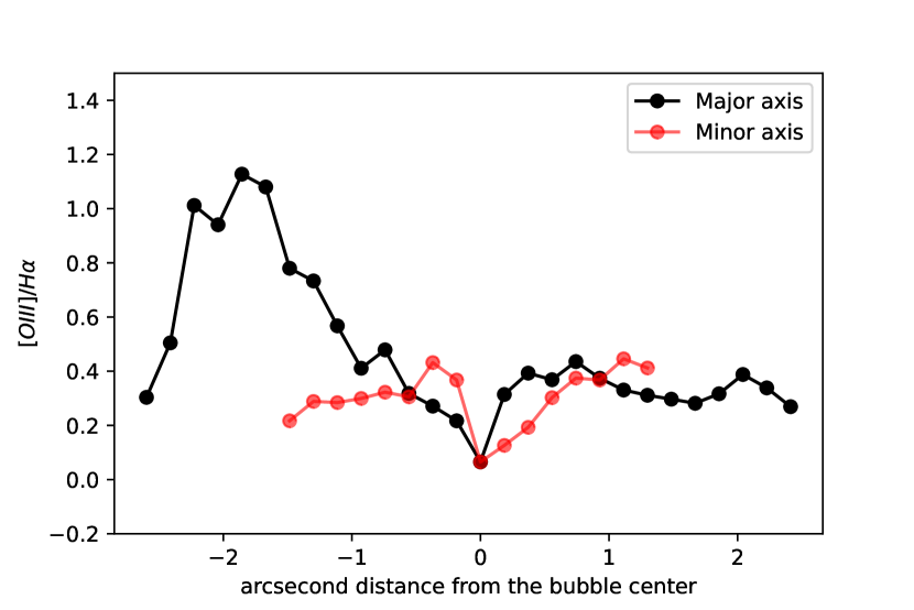
Figure 7: The spatial profile of the [O iii]/H$\alpha$ flux ratio along the major and minor axes of the extended nebula (see the white bars in Figure 6).

The shock-ionized bubbles around ULXs can be formed via two mechanisms: through explosive events like supernovae (i.e., supernova remnants) or being inflated by continuous jet/outflow from ULXs (Pakull et al., 2006). However, ULX bubbles often have sizes of a few hundred pc (e.g., Ramsey et al., 2006; Grisé et al., 2011), which are one order of magnitude larger than normal supernova remnants. Although there exists the possibility of very energetic hypernova explosions, it is unlikely considering the stellar environments and the survival of ULXs as binary systems during the events (Feng & Soria, 2011). Therefore, we suggest the H$\alpha$ bubble structure around X4 is more likely to be inflated by the ULX jet/outflow.

It is worth noting that, unlike many other ULX bubbles, this extended structure around X4 only has a one-sided lobe to the southwest direction, while X4 itself is close to the east edge of the bubble. The missing of the lobe in the other direction is not caused by the relativistic beaming because the bubble expansion velocity $v_{s}$ is only at the order of hundred $\rm km\ s^{-1}$, far below the speed of light. For example, the bubble around the ULX in NGC 5585 has an expansion velocity of $125\ \rm km\ s^{-1}$ (Soria et al., 2021). For this bubble around X4, the expansion velocity is estimated to be $v_{s}\sim 110$ $\rm km\ s^{-1}$ (see Section 5.2).

The asymmetric profile of an extended nebula could imply the density gradient of ISM or outflows, as suggested for IC 342 X-1 (Cseh et al., 2012). Here in our case, one viable scenario is that the ISM is much denser to the east of X4, resulting in an outflow blocked by the dense medium. Hence, the east area is mainly photoionized by the ULX itself (as shown by the [O iii]/H$\beta$ ratio profile), while most other regions are dominated by shock ionization through the outflow. Similar situations can be found in the simulations of supernova feedback (Creasey et al., 2011; Pardi, 2017). In their simulations, if the ISM density reaches $10^{2}$–$10^{4}$ cm^-3 and the ejection temperature is lower than 10⁶ K, the injected energy of the outflow will be immediately lost due to the strong radiative cooling in the high density regions, dubbed the overcooling problem.

An alternative interpretation of this unusual morphology is that the accretion disk of X4 has launched an asymmetric outflow, i.e., the outflow to the east direction is much weaker or nonexistent. There have been numerical simulations showing that an asymmetric or even one-sided outflow can be formed from the accretion disk if the accretor is rotating and is accompanied with a complex magnetic field (Lovelace et al., 2010; Dyda et al., 2015).

It is also possible that both of the two mechanisms are responsible for this asymmetric morphology. The side with the weaker/absent outflow has more dense ambient ISM, leading to photoionization dominating the compact east area close to the ULX, while the shock-ionized bubble is only formed to the opposite direction.

5.2 Mechanical Power Estimation

To estimate the mechanical power needed to inflate the bubble, we first calculate the H$\alpha$ luminosity from the surface brightness of the structure measured with Python/Photutils. The brightest region in the H$\alpha$ band (marked with “A” in Figure 3) has a surface brightness of $19.34\pm 0.01$ mag arcsec^-2. The whole bubble structure, which is confined in a donut shape (region B in Figure 3, subtracting region C while including region A), has an average surface brightness of 19.64 $\pm$ 0.01 mag arcsec^-2. Using the surface brightness and bubble size $R$, We can estimate the injected mechanical power $P_{w}$.

Based on the standard bubble theory (Weaver et al., 1977; Pakull et al., 2006), $P_{w}$ can be calculated as

$$P_{39}\approx 3.8{R_{2}}^{2}{v_{2}}^{3}n\ \rm{erg\ s^{-1}},$$ (2)

where $P_{39}\equiv P_{w}/(10^{39}\ \rm erg\ s^{-1})$; $R_{2}\equiv R/(100\ \rm pc)$; $v_{2}\equiv v_{s}/(100\ \rm km\ s^{-1})$; $n$ is the ISM number density in unit of cm^-3. As the ULX is located at the edge of the $H\alpha$ bubble, we conceive that the one-sided jet/wind formed this one-lobe bubble. Therefore, we adopt the scale of the whole bubble to substitute the radius, i.e., $R=130\ \rm pc$ and $R_{2}=1.3$. The number density $n$ can be derived from the H$\beta$ luminosity $L_{H\beta}$, the expanding velocity $v_{s}$, and the area of the spherical bubble $A$ (Dopita & Sutherland, 1996),

$$n=1.3\times 10^{5}L_{H\beta}A^{-1}v_{2}^{-2.41}\ \rm cm^{-3}.$$ (3)

The surface area $A$ of the spherical bubble with a diameter of 130 pc is calculated as $5\times 10^{41}$ cm². Without available H$\beta$ imaging, the H$\beta$ luminosity can be derived from H$\alpha$ luminosity using the Balmer line ratio $\tau$. The intrinsic H$\alpha$ luminosity is $L_{H\alpha}=1.2\times 10^{38}$ erg s^-1, calculated from the bubble surface brightness. With the lack of optical spectroscopy on the bubble, the precise expanding velocity $v_{s}$ is not available. We employed the widely used shock-ionization model MAPPINGS V (Allen et al., 2008) to estimate $\tau$ and $v_{s}$. We carried out a series of calculations with MAPPINGS V which returned values for a variety of line ratios to compare with the observation. We fixed the metallicity to 0.5 solar abundance (Pilyugin et al., 2014), magnetic field to a typical value of 0.3 $\mu$G, and arranged a large input grid of the shock velocity $v_{s}$ and hydrogen number density $n$, finding a set of solution matching the observed [O iii]/H$\alpha$ line ratio, which is $\approx 0.3$ along the most parts of the H$\alpha$ bubble (see Figure 7). The result is shown in Figure 8. We obtained the following parameter values in this solution: $n\sim 6\ {\rm cm^{-3}},v_{s}\sim 110\ \rm{km\ s^{-1}}$, and the Balmer line ratio $\tau\sim 3.75$.

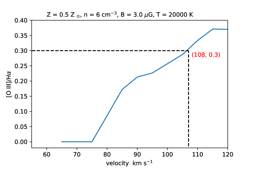
Figure 8: The adopted solution from MAPPING V code. The ISM number density is $6\ \rm cm^{-3}$. When the shock velocity $v_{s}\ \approx$ 108 $\rm{km\ s^{-1}}$, the [O iii]/H$\alpha$ flux ratio is consistent with the observed value of $\approx 0.3$.

Combining Eqns. (2) and (3), we can derive a relation where the mechanical power $P_{w}$ is determined by the H$\alpha$ luminosity $L_{H\alpha}$, the line ratio $\tau$ and expanding velocity $v_{s}$:

$$P_{39}\approx 5.0\times 10^{5}R_{2}^{2}(L_{H\alpha}/\tau)A^{-1}v_{2}^{0.59}.$$ (4)

By substituting the MAPPING V solution, we calculated the value of $P_{39}\approx 51$, i.e., the injected mechanical power $P_{w}\sim 5\times 10^{40}$ erg s^-1. The lifetime $t$ of the bubble is estimated to be $t=\frac{3}{5}R/v_{s}\sim 7\times 10^{5}$ yr.

We can now calculate the mass-loss rate $\dot{M}$ of the ULX jet/wind. In the non- and mildly-relativistic scenario, the injected power can also be expressed as $P_{w}=\frac{1}{2}\dot{M}v_{w}^{2}$ (Weaver et al., 1977), where $v_{w}$ is the velocity of jet/wind. This equation can be transformed to

$$\dot{M}\approx 3.3\times 10^{-8}P_{39}/v^{2}_{c}\ \ M_{\odot}\ {\rm yr}^{-1},$$ (5)

where $v_{c}(\equiv v_{w}/c)$ is the wind velocity in unit of the speed of light $c$. The left panel of Figure 9 shows the range of the mass-loss rate $\dot{M}$ and its dependence on wind velocity $v_{c}$. With a typical value of $v_{c}\sim 0.2$ (Pinto et al., 2016, 2021; Kosec et al., 2018), the mass-loss rate is calculated as $\sim 10^{-5}M_{\odot}\ {\rm yr}^{-1}$ (the green vertical line in the left panel of Figure 9), which means that $\sim 10\ M_{\odot}$ will be lost through ULX wind in the bubble lifetime. Such a high mass loss rate will make it difficult to sustain the long-term stable accretion activity.

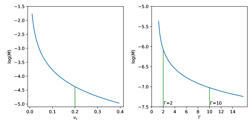
Figure 9: The estimated mass-loss rate $\dot{M}$ of non- and mildly-relativistic wind (left panel) and the relativistic jet (right panel). The $x$-axis is the wind velocity normalized by the speed of light $v_{c}$ in the left panel and the bulk Lorentz factor $\Gamma$ in the right panel.

Instead, we consider the jet-powered bubble scenario with highly relativistic ejection velocity. The mass-loss rate $\dot{M}$ can be inferred with the following equation (Kaiser & Alexander, 1997; Cseh et al., 2012),

$$\dot{M}=\frac{P_{w}}{(\Gamma-1)c^{2}}.$$ (6)

Adopting a minimum bulk Lorentz factor $\Gamma=2$, we can derive the $\dot{M}$ ranges as $\sim 10^{-6}\ M_{\odot}\ \rm yr^{-1}$, while for a higher bulk Lorentz factor, like $\Gamma=10$, the mass-loss rate would decrease to $\sim 10^{-7}\ M_{\odot}\ \rm yr^{-1}$ (Figure 9 right panel), which is clearly more realistic for sustaining the accretion of ULXs. This would suggest that relativistic jets are necessary to generate the shock-ionized ULX bubbles like the one we found around X4. Mildly-relativistic winds with typical velocity of $\sim 0.2c$ alone would not provide adequate mechanical power. Steady jets at the distance of NGC 4631 would have a radio flux level of $\sim 1\ \mu$Jy, which is difficult to detect with current facilities, while flaring jets that are 1–2 orders of magnitude brighter could be detected with, e.g., the Karl G. Jansky Very Large Array (VLA), like the case of Holmberg II X-1 (Cseh et al., 2015). We have searched the VLA database; sensitive radio imaging data with sub-arcsec resolution on NGC 4631 will be publicly available in the near future.

The estimated jet mechanical power of NGC 4631 X4 is greater than its radiative luminosity. It would also be above the Eddington limit if the accretor mass is less than $\sim 100\ M_{\odot}$, as for most ULXs. This is similar to the cases of several microquasars found in nearby galaxies, e.g., NGC 7793 S26 (Pakull et al., 2010) and M83 MQ1 (Soria et al., 2014), both of which have the same level of jet power at $\sim 10^{40}$ erg s^-1. The Galactic microquasar SS 433 also has the jet power far exceeding its X-ray luminosity (Fabrika, 2004). These microquasars also have surrounding shock-ionized bubble structures detected with optical/infrared emission lines. Their X-ray luminosity are admittedly orders of magnitude below the canonical definition of ULXs. However, they could have had episodes of super-Eddington radiative luminosity in the past, while NGC 4631 X4 itself also had sub-Eddington X-ray luminosity ($\sim 10^{37}$ erg s^-1) during its Chandra observation. Furthermore, the low X-ray luminosity of SS 433 is also due to the heavy obscuration along the line of sight; only reflected X-ray flux is detectable (e.g., Begelman et al. 2006; Middleton et al. 2021). On a much larger scale, some powerful Fanaroff-Riley II radio galaxies and blazars have been found to have jet power much greater than the radiative luminosity (Ito et al., 2008; Ghisellini et al., 2014). NGC 4631 X4 and the aforementioned microquasars appears to be analogs of these active galaxies at stellar scales.

From another perspective, we consider the energy sources of the injected mechanical power. In case of all the jet mechanical power originates from the accretion, i.e., the release of gravitational potential energy of the accreted material, the needed accretion rate $\dot{m}$ can be calculated from $P_{w}=\epsilon\dot{m}c^{2}$., where $\epsilon$ is the fraction of accretion power converted into mechanical energy. Under the assumption of $\epsilon=0.1$, which is already considered as exceptionally high, the needed accretion rate is $\dot{m}\sim 10^{-5}\ M_{\odot}\ \rm yr^{-1}$. For more realistic $\epsilon$ values, the needed accretion rate would be even higher. This would suggest that there should be additional source(s) of the jet mechanical power. For the cases of black hole accretion, a promising energy source would be the black hole spin, i.e., the Blandford-Znejak (BZ) mechanism (Blandford & Znajek, 1977). There have been evidences supporting this jet power origin for Galactic black hole binaries (e.g., Narayan & McClintock 2012; but also see, e.g., Russell et al. 2013). From our analyses for NGC 4631 X4, the presumable jet requires additional energy source besides the accretion to provide sufficient mechanical power to inflate the bubble structure. Numerical simulations on super-Eddington accretions by Narayan et al. (2017) demonstrate that the total energy conversion efficiency (including both radiative and mechanical power) of ULXs can be as high as $\sim 0.7$ when introducing the high black hole spin ($a_{*}=0.9$) and the “magnetic arrested disk” (MAD; e.g., Bisnovatyi-Kogan & Ruzmaikin 1976; Narayan et al. 2003) models, where the majority of energy is carried out in the form of mechanical power. The black hole spin energy is extracted into the jets via the BZ mechanism.

6 Conclusions

We present an optical imaging study of the five brightest X-ray sources in NGC 4631, among which Soria & Ghosh (2009) identified four ULXs (X1, X2, X4, X5). Chandra/ACIS data are utilized to obtain precise astrometry and to identify possible optical counterparts from the HST/ACS images. A broad-band and narrow-band imaging campaign with CFHT/MegaCam is carried out to search for the bubble structures around the X-ray sources and to investigate their accretion states.

The supersoft X1 has a large optical-to-X-ray positional error ($\approx 0\farcs 5$) due to its low counts during the Chandra observation. The candidate optical counterparts and the surrounding stars of X1 span a wide range of ages from 5 Myr to 80 Myr in the CMD, suggesting that they are likely not physically associated. X3 resides in a stellar environment with the age range of $\sim 50$–80 Myr, while its three candidate counterparts show similar ages. X4 has six optical counterpart candidates, all of which show the age range consistent with that of the surrounding stars at $\sim 20$–80 Myr. X5 appears to be associated with a star group with the age of $\sim 5$–10 Myr, which is typical for the star clusters related to ULXs (Poutanen et al., 2013). This young star group is a manifestation of the strong star forming activity in the starburst galaxy NGC 4631. We do not provide the CMD for X2 due to its high extinction.

A bubble nebula with a size of $\sim 130$ pc $\times$ 100 pc around X4 is firstly detected in our CFHT/MegaCam H$\alpha$ narrow-band image. Unlike many other ULXs residing in the interior of their respective bubbles, this ULX is located at the east edge. It appears the H$\alpha$ bubble originates from X4 and expands one-sided towards the west direction, reaching maximum luminosity in the outermost region. In contrast, the extended structure appears smaller in the [O iii] image, while its brightest section is much closer to the ULX and located to the east. The [O iii]/H$\alpha$ line ratio map suggests that the H$\alpha$ bubble is generated mainly by shock ionization, while the [O iii] structure is illuminated by the ULX via photoionization.

The X4 bubble has an average surface brightness of $19.64\pm 0.01$ mag arcsec^-2 in the H$\alpha$ band. By matching the observed [O iii]/H$\alpha$ line ratio, we estimate the bubble expansion velocity $v_{s}\sim 110$ km s^-1 and the ambient ISM density $n\sim 6$ cm^-3 using the MAPPINGS V code. With these parameters, we constrain the mechanical power to inflate the bubble being $\sim 5\times 10^{40}$ erg s^-1 and the bubble age of $\sim 7\times 10^{5}$ yr. Furthermore, we demonstrate that for non- or mildly- relativistic wind alone to generate the observed bubble, the needed mass-loss rate would be too high to sustain the long-term accretion. Instead, in the case of a relativistic jet (with a bulk Lorentz factor $\Gamma\sim 10$) to inflate the bubble, the mass-loss rate would decrease to a more realistic level of $\sim 10^{-7}\ M_{\odot}\ \rm yr^{-1}$. Similar to the cases of a few microquasars found in the Milky Way and nearby galaxies (e.g., SS 433, NGC 7793 S26, and M83 MQ1), the estimated mechanical jet power of NGC 4631 X4 is above the Eddington limit for a stellar-mass black hole. The black hole spin is likely to contribute to the jet power via the BZ mechanism.

For future perspectives, optical spectroscopy, especially those with the integral-field instruments, will provide the bubble expansion velocity field and flux ratio map for a variety of emission lines, from which a more precise estimate of the mechanical power can be obtained. High-resolution X-ray spectroscopy will enable the measurement of outflow velocity, while deeper radio imaging with high angular resolution could reveal the ULX jet. With all these combined, we can derive a more reliable mass-loss rate of the outflow and further constrain the accretion models of ULXs.

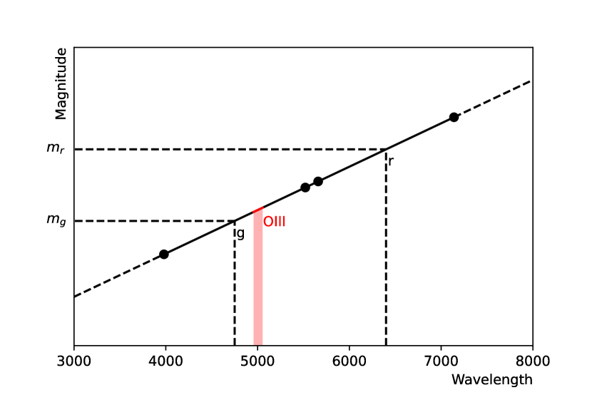
Figure 10: The supposed linear relation between continuum magnitude and wavelength. The two pairs of black dots mark the boarders of the $g$ and $r$ bands of CFHT/MegaCam. The continuum in the [O iii] band is illustrated by the red shaded area.

Appendix A Subtracting the continuum from the [O iii] band images

To remove the $g$-band contribution from the [O iii] images, we assume the magnitude of continuum at a given wavelength is linearly correlated to this wavelength $\lambda$ in the range of the $g$ and $r$ bands (Figure 10), i.e., the continuum follows a power-law spectral model ($f\propto\lambda^{-\alpha}$). Then the $g$-band part in [O iii] can be described in the equation,

$$\frac{m_{r}-m_{g}}{\lambda_{r}-\lambda_{g}}=\frac{m_{g/\rm O\sc III}-m_{g}}{\lambda_{\rm O\sc III}-\lambda_{g}}.$$ (A1)

With replacing the corresponding central wavelength in the filters of Megacam ($\lambda_{g}$ = 4750  Å, $\lambda_{\rm O\sc III}$ = 5006  Å, $\lambda_{r}$ = 6400 Å), the equation can be transformed to,

$$m_{g/\rm O\sc III}\ \approx\ m_{g}-0.155\times(m_{g}-m_{r}).$$ (A2)

It is worth noting that this relation is only valid to the images generated by MegaPipe for which the counts have been normalized for each band. The continuum component for each pixel can be derived after the equation is applied pixel by pixel.

References

- Allen et al. (2008) Allen, M. G., Groves, B. A., Dopita, M. A., Sutherland, R. S., & Kewley, L. J. 2008, The Astrophysical Journal Supplement Series, 178, 20
- Astropy Collaboration et al. (2013) Astropy Collaboration, Robitaille, T. P., Tollerud, E. J., et al. 2013, A&A, 558, A33, doi: 10.1051/0004-6361/201322068
- Astropy Collaboration et al. (2018) Astropy Collaboration, Price-Whelan, A. M., Sipőcz, B. M., et al. 2018, AJ, 156, 123, doi: 10.3847/1538-3881/aabc4f
- Bachetti et al. (2014) Bachetti, M., Harrison, F. A., Walton, D. J., et al. 2014, Nature, 514, 202, doi: 10.1038/nature13791
- Begelman et al. (2006) Begelman, M. C., King, A. R., & Pringle, J. E. 2006, MNRAS, 370, 399. doi:10.1111/j.1365-2966.2006.10469.x
- Bertin (2006) Bertin, E. 2006, in Astronomical Society of the Pacific Conference Series, Vol. 351, Astronomical Data Analysis Software and Systems XV, ed. C. Gabriel, C. Arviset, D. Ponz, & S. Enrique, 112
- Bertin (2010) Bertin, E. 2010, SWarp: Resampling and Co-adding FITS Images Together. http://ascl.net/1010.068
- Bertin & Arnouts (1996) Bertin, E., & Arnouts, S. 1996, A&AS, 117, 393, doi: 10.1051/aas:1996164
- Bisnovatyi-Kogan & Ruzmaikin (1976) Bisnovatyi-Kogan, G. S., & Ruzmaikin, A. A. 1976, Ap&SS, 42, 401, doi: 10.1007/BF01225967
- Blandford & Znajek (1977) Blandford, R. D., & Znajek, R. L. 1977, MNRAS, 179, 433, doi: 10.1093/mnras/179.3.433
- Boselli et al. (2018) Boselli, A., Fossati, M., Ferrarese, L., et al. 2018, A&A, 614, A56, doi: 10.1051/0004-6361/201732407
- Bressan et al. (2012) Bressan, A., Marigo, P., Girardi, L., et al. 2012, Monthly Notices of the Royal Astronomical Society, 427, 127
- Cardelli et al. (1989) Cardelli, J. A., Clayton, G. C., & Mathis, J. S. 1989, ApJ, 345, 245, doi: 10.1086/167900
- Carpano et al. (2018) Carpano, S., Haberl, F., Maitra, C., & Vasilopoulos, G. 2018, MNRAS, 476, L45, doi: 10.1093/mnrasl/sly030
- Creasey et al. (2011) Creasey, P., Theuns, T., Bower, R. G., & Lacey, C. G. 2011, MNRAS, 415, 3706, doi: 10.1111/j.1365-2966.2011.19001.x
- Cseh et al. (2012) Cseh, D., Corbel, S., Kaaret, P., et al. 2012, ApJ, 749, 17, doi: 10.1088/0004-637X/749/1/17
- Cseh et al. (2015) Cseh, D., Miller-Jones, J. C. A., Jonker, P. G., et al. 2015, MNRAS, 452, 24, doi: 10.1093/mnras/stv1308
- Cutri et al. (2021) Cutri, R. M., Wright, E. L., Conrow, T., et al. 2021, VizieR Online Data Catalog, II/328
- Dolphin (2000) Dolphin, A. E. 2000, Publications of the Astronomical Society of the Pacific, 112, 1383
- Dopita & Sutherland (1996) Dopita, M. A., & Sutherland, R. S. 1996, ApJS, 102, 161, doi: 10.1086/192255
- Dyda et al. (2015) Dyda, S., Lovelace, R. V. E., Ustyugova, G. V., et al. 2015, MNRAS, 450, 481, doi: 10.1093/mnras/stv623
- Eckart et al. (2005) Eckart, M. E., Laird, E. S., Stern, D., et al. 2005, ApJS, 156, 35, doi: 10.1086/425869
- Evans et al. (2010) Evans, I. N., Primini, F. A., Glotfelty, K. J., et al. 2010, ApJS, 189, 37. doi: 10.1088/0067-0049/189/1/37
- Fabrika (2004) Fabrika, S. 2004, Astrophys. Space Phys. Res., 12, 1. https://arxiv.org/abs/astro-ph/0603390
- Farrell et al. (2009) Farrell, S. A., Webb, N. A., Barret, D., Godet, O., & Rodrigues, J. M. 2009, Nature, 460, 73, doi: 10.1038/nature08083
- Feng & Soria (2011) Feng, H., & Soria, R. 2011, New A Rev., 55, 166, doi: 10.1016/j.newar.2011.08.002
- Flewelling (2018) Flewelling, H. 2018, in American Astronomical Society Meeting Abstracts, Vol. 231, American Astronomical Society Meeting Abstracts #231, 436.01
- Flewelling et al. (2020) Flewelling, H. A., Magnier, E. A., Chambers, K. C., et al. 2020, ApJS, 251, 7, doi: 10.3847/1538-4365/abb82d
- Ford et al. (1998) Ford, H. C., Bartko, F., Bely, P. Y., et al. 1998, in Society of Photo-Optical Instrumentation Engineers (SPIE) Conference Series, Vol. 3356, Space Telescopes and Instruments V, ed. P. Y. Bely & J. B. Breckinridge, 234–248, doi: 10.1117/12.324464
- Fruscione et al. (2006) Fruscione, A., McDowell, J. C., Allen, G. E., et al. 2006, in Society of Photo-Optical Instrumentation Engineers (SPIE) Conference Series, Vol. 6270, Society of Photo-Optical Instrumentation Engineers (SPIE) Conference Series, ed. D. R. Silva & R. E. Doxsey, 62701V, doi: 10.1117/12.671760
- Fürst et al. (2016) Fürst, F., Walton, D. J., Harrison, F. A., et al. 2016, ApJ, 831, L14, doi: 10.3847/2041-8205/831/2/L14
- Ghisellini et al. (2014) Ghisellini, G., Tavecchio, F., Maraschi, L., Celotti, A., & Sbarrato, T. 2014, Nature, 515, 376, doi: 10.1038/nature13856
- Gladstone et al. (2009) Gladstone, J. C., Roberts, T. P., & Done, C. 2009, MNRAS, 397, 1836, doi: 10.1111/j.1365-2966.2009.15123.x
- Grisé et al. (2011) Grisé, F., Kaaret, P., Pakull, M. W., & Motch, C. 2011, ApJ, 734, 23, doi: 10.1088/0004-637X/734/1/23
- Gúrpide et al. (2022) Gúrpide, A., Parra, M., Godet, O., Contini, T., & Olive, J.-F. 2022, arXiv e-prints, arXiv:2201.09333. https://arxiv.org/abs/2201.09333
- Güver & Özel (2009) Güver, T., & Özel, F. 2009, MNRAS, 400, 2050, doi: 10.1111/j.1365-2966.2009.15598.x
- Gwyn (2008) Gwyn, S. D. J. 2008, PASP, 120, 212, doi: 10.1086/526794
- Harris et al. (2020) Harris, C. R., Millman, K. J., van der Walt, S. J., et al. 2020, Nature, 585, 357, doi: 10.1038/s41586-020-2649-2
- Hong et al. (2005) Hong, J., van den Berg, M., Schlegel, E. M., et al. 2005, ApJ, 635, 907. doi: 10.1086/496966
- Hunter (2007) Hunter, J. D. 2007, Computing in Science and Engineering, 9, 90, doi: 10.1109/MCSE.2007.55
- Irwin et al. (2011) Irwin, J. A., Wilson, C. D., Wiegert, T., et al. 2011, MNRAS, 410, 1423, doi: 10.1111/j.1365-2966.2010.17510.x
- Israel et al. (2017a) Israel, G. L., Belfiore, A., Stella, L., et al. 2017a, Science, 355, 817, doi: 10.1126/science.aai8635
- Israel et al. (2017b) Israel, G. L., Papitto, A., Esposito, P., et al. 2017b, MNRAS, 466, L48, doi: 10.1093/mnrasl/slw218
- Ito et al. (2008) Ito, H., Kino, M., Kawakatu, N., Isobe, N., & Yamada, S. 2008, ApJ, 685, 828, doi: 10.1086/591036
- Kaaret et al. (2017) Kaaret, P., Feng, H., & Roberts, T. P. 2017, ARA&A, 55, 303, doi: 10.1146/annurev-astro-091916-055259
- Kaiser & Alexander (1997) Kaiser, C. R., & Alexander, P. 1997, MNRAS, 286, 215, doi: 10.1093/mnras/286.1.215
- Kosec et al. (2018) Kosec, P., Pinto, C., Walton, D. J., et al. 2018, MNRAS, 479, 3978, doi: 10.1093/mnras/sty1626
- Kosec et al. (2021) Kosec, P., Pinto, C., Reynolds, C. S., et al. 2021, MNRAS, 508, 3569, doi: 10.1093/mnras/stab2856
- Liu et al. (2013) Liu, J.-F., Bregman, J. N., Bai, Y., Justham, S., & Crowther, P. 2013, Nature, 503, 500, doi: 10.1038/nature12762
- Lovelace et al. (2010) Lovelace, R. V. E., Romanova, M. M., Ustyugova, G. V., & Koldoba, A. V. 2010, MNRAS, 408, 2083, doi: 10.1111/j.1365-2966.2010.17284.x
- Magnier & Cuillandre (2004) Magnier, E. A., & Cuillandre, J. C. 2004, PASP, 116, 449, doi: 10.1086/420756
- Meléndez et al. (2015) Meléndez, M., Veilleux, S., Martin, C., et al. 2015, ApJ, 804, 46, doi: 10.1088/0004-637X/804/1/46
- Middleton et al. (2021) Middleton, M. J., Walton, D. J., Alston, W., et al. 2021, MNRAS, 506, 1045. doi:10.1093/mnras/stab1280
- Mineo et al. (2012) Mineo, S., Gilfanov, M., & Sunyaev, R. 2012, MNRAS, 419, 2095, doi: 10.1111/j.1365-2966.2011.19862.x
- Moon et al. (2011) Moon, D.-S., Harrison, F. A., Cenko, S. B., et al. 2011, ApJ, 731, L32. doi: 10.1088/2041-8205/731/2/L32
- Motch et al. (2014) Motch, C., Pakull, M. W., Soria, R., Grisé, F., & Pietrzyński, G. 2014, Nature, 514, 198, doi: 10.1038/nature13730
- Narayan et al. (2003) Narayan, R., Igumenshchev, I. V., & Abramowicz, M. A. 2003, PASJ, 55, L69, doi: 10.1093/pasj/55.6.L69
- Narayan & McClintock (2012) Narayan, R., & McClintock, J. E. 2012, MNRAS, 419, L69, doi: 10.1111/j.1745-3933.2011.01181.x
- Narayan et al. (2017) Narayan, R., Sa̧dowski, A., & Soria, R. 2017, MNRAS, 469, 2997, doi: 10.1093/mnras/stx1027
- Pakull et al. (2006) Pakull, M. W., Grise, F., & Motch, C. 2006, Proceedings of the International Astronomical Union, 1, 293
- Pakull & Mirioni (2002) Pakull, M. W., & Mirioni, L. 2002, arXiv e-prints, astro. https://arxiv.org/abs/astro-ph/0202488
- Pakull et al. (2010) Pakull, M. W., Soria, R., & Motch, C. 2010, Nature, 466, 209, doi: 10.1038/nature09168
- Pardi (2017) Pardi, A.-L. 2017, PhD thesis, LMU Munich, Germany
- Pilyugin et al. (2014) Pilyugin, L. S., Grebel, E. K., & Kniazev, A. Y. 2014, AJ, 147, 131, doi: 10.1088/0004-6256/147/6/131
- Pinto et al. (2016) Pinto, C., Middleton, M. J., & Fabian, A. C. 2016, Nature, 533, 64, doi: 10.1038/nature17417
- Pinto et al. (2021) Pinto, C., Soria, R., Walton, D. J., et al. 2021, MNRAS, 505, 5058, doi: 10.1093/mnras/stab1648
- Poutanen et al. (2013) Poutanen, J., Fabrika, S., Valeev, A. F., Sholukhova, O., & Greiner, J. 2013, MNRAS, 432, 506, doi: 10.1093/mnras/stt487
- Qiu & Feng (2021) Qiu, Y., & Feng, H. 2021, ApJ, 906, 36, doi: 10.3847/1538-4357/abc959
- Quintin et al. (2021) Quintin, E., Webb, N. A., Gúrpide, A., Bachetti, M., & Fürst, F. 2021, MNRAS, 503, 5485, doi: 10.1093/mnras/stab814
- Ramsey et al. (2006) Ramsey, C. J., Williams, R. M., Gruendl, R. A., et al. 2006, ApJ, 641, 241, doi: 10.1086/499070
- Roberts et al. (2008) Roberts, T. P., Levan, A. J., & Goad, M. R. 2008, MNRAS, 387, 73, doi: 10.1111/j.1365-2966.2008.13293.x
- Rodríguez Castillo et al. (2020) Rodríguez Castillo, G. A., Israel, G. L., Belfiore, A., et al. 2020, ApJ, 895, 60, doi: 10.3847/1538-4357/ab8a44
- Russell et al. (2013) Russell, D. M., Gallo, E., & Fender, R. P. 2013, MNRAS, 431, 405, doi: 10.1093/mnras/stt176
- Salvaggio et al. (2022) Salvaggio, C., Wolter, A., Pintore, F., et al. 2022, MNRAS, 512, 1814, doi: 10.1093/mnras/stac559
- Sathyaprakash et al. (2019) Sathyaprakash, R., Roberts, T. P., Walton, D. J., et al. 2019, MNRAS, 488, L35, doi: 10.1093/mnrasl/slz086
- Schlafly & Finkbeiner (2011) Schlafly, E. F., & Finkbeiner, D. P. 2011, ApJ, 737, 103, doi: 10.1088/0004-637X/737/2/103
- Science Software Branch at STScI (2012) Science Software Branch at STScI. 2012, PyRAF: Python alternative for IRAF, Astrophysics Source Code Library, record ascl:1207.011. http://ascl.net/1207.011
- Soria & Ghosh (2009) Soria, R., & Ghosh, K. K. 2009, ApJ, 696, 287, doi: 10.1088/0004-637X/696/1/287
- Soria et al. (2014) Soria, R., Long, K. S., Blair, W. P., et al. 2014, Science, 343, 1330, doi: 10.1126/science.1248759
- Soria et al. (2010) Soria, R., Pakull, M. W., Broderick, J. W., Corbel, S., & Motch, C. 2010, MNRAS, 409, 541, doi: 10.1111/j.1365-2966.2010.17360.x
- Soria et al. (2021) Soria, R., Pakull, M. W., Motch, C., et al. 2021, MNRAS, 501, 1644, doi: 10.1093/mnras/staa3784
- Tao et al. (2011) Tao, L., Feng, H., Grisé, F., & Kaaret, P. 2011, ApJ, 737, 81, doi: 10.1088/0004-637X/737/2/81
- Virtanen et al. (2020) Virtanen, P., Gommers, R., Oliphant, T. E., et al. 2020, Nature Methods, 17, 261, doi: 10.1038/s41592-019-0686-2
- Walton et al. (2014) Walton, D. J., Harrison, F. A., Grefenstette, B. W., et al. 2014, ApJ, 793, 21, doi: 10.1088/0004-637X/793/1/21
- Wang et al. (2016) Wang, S., Liu, J., Qiu, Y., et al. 2016, ApJS, 224, 40, doi: 10.3847/0067-0049/224/2/40
- Weaver et al. (1977) Weaver, R., McCray, R., Castor, J., Shapiro, P., & Moore, R. 1977, ApJ, 218, 377, doi: 10.1086/155692
- Webb et al. (2012) Webb, N., Cseh, D., Lenc, E., et al. 2012, Science, 337, 554, doi: 10.1126/science.1222779
- Weng & Feng (2018) Weng, S.-S., & Feng, H. 2018, ApJ, 853, 115, doi: 10.3847/1538-4357/aaa45c
- Weng et al. (2017) Weng, S.-S., Ge, M.-Y., Zhao, H.-H., et al. 2017, ApJ, 843, 69, doi: 10.3847/1538-4357/aa76ec
- Wes McKinney (2010) Wes McKinney. 2010, in Proceedings of the 9th Python in Science Conference, ed. Stéfan van der Walt & Jarrod Millman, 56 – 61, doi: 10.25080/Majora-92bf1922-00a
- Williams et al. (2014) Williams, B. F., Lang, D., Dalcanton, J. J., et al. 2014, The Astrophysical Journal Supplement Series, 215, 9
- Wilson-Hodge et al. (2018) Wilson-Hodge, C. A., Malacaria, C., Jenke, P. A., et al. 2018, ApJ, 863, 9, doi: 10.3847/1538-4357/aace60
- Yamasaki et al. (2009) Yamasaki, N. Y., Sato, K., Mitsuishi, I., & Ohashi, T. 2009, PASJ, 61, S291, doi: 10.1093/pasj/61.sp1.S291
- Yang et al. (2011) Yang, L., Feng, H., & Kaaret, P. 2011, ApJ, 733, 118, doi: 10.1088/0004-637X/733/2/118
- Zhao et al. (2005) Zhao, P., Grindlay, J. E., Hong, J. S., et al. 2005, ApJS, 161, 429. doi: 10.1086/497095
- Zhou et al. (2022) Zhou, C., Bian, F., Feng, H., & Huang, J. 2022, ApJ, 935, 38, doi: 10.3847/1538-4357/ac815f
- Zhou et al. (2019) Zhou, Y., Feng, H., Ho, L. C., & Yao, Y. 2019, ApJ, 871, 115, doi: 10.3847/1538-4357/aaf724