From higher order free cumulants to non-separable hypermaps

Abstract

Higher order free moments and cumulants, introduced by Collins, Mingo, Śniady and Speicher in 2006, describe the fluctuations of unitarily invariant random matrices in the limit of infinite size. The functional relations between their generating functions were only found last year by Borot, Garcia-Failde, Charbonnier, Leid and Shadrin and a combinatorial derivation is still missing. We simplify these relations and show how their combinatorial derivation reduces to the computation of generating functions of planar non-separable hypermaps with prescribed vertex valencies and weighted hyper-edges. The functional relations obtained by Borot et al. involve some remarkable simplifications, which can be formulated as identities satisfied by these generating functions. The case of third order free cumulants, whose combinatorial understanding was already out of reach, is derived explicitly.

1 Introduction

First order free probability [24, 22, 21, 20, 6] provides an efficient understanding of expectations of traces of $N\times N$ random matrices $B$ at leading order in the limit of infinite size $N$:

$$\varphi(b^{\lambda})=\lim_{N\rightarrow\infty}\frac{1}{N}\,\mathbb{E}\mathrm{Tr}(B^{\lambda}),$$

in generalizing the concepts of independence, cumulants, convolution, and so on, to freeness, free cumulants, free convolution… A central role is played by the free cumulants $\kappa_{\lambda}[b]$, whose knowledge is equivalent to the asymptotic moments $\varphi(b^{\lambda})$ through the free moment-cumulant formulas, which involve summations over non-crossing partitions and are thus invertible in the associated lattice. Free cumulants are the useful tools for computing the asymptotic spectrum of a sum or product of independent random matrices, for instance. In practice however, such computations are rendered efficient by going to generating functions of moments and cumulants, and using the functional analog of these free moment-cumulant formulas, allowing for the use of complex analysis.

Higher order free probability [17, 18, 19, 9] deals with the fluctuations of random matrices, that is, with the connected correlations of their traces at leading order in the limit $N\rightarrow\infty$:

$$\varphi(b^{\lambda_{1}},\ldots,b^{\lambda_{p}})=\lim_{N\rightarrow\infty}N^{p-2}k_{p}\bigl{(}\mathrm{Tr}(B^{\lambda_{1}}),\ldots,\mathrm{Tr}(B^{\lambda_{p}})\bigr{)},$$

where $k_{p}$ is the $p$-th classical cumulant (connected correlation). The role of free cumulants is then played by their higher order counterparts, $\kappa_{\lambda_{1},\ldots,\lambda_{p}}[b]$, and the notion of freeness generalizes to higher order freeness. These quantities are related to the $\varphi(b^{\lambda_{1}},\ldots,b^{\lambda_{p}})$ by higher-order free moment-cumulant formulas, also invertible, and which involve summations over pairs consisting of a permutation of $n=\sum_{i}\lambda_{i}$ elements, and a partition of its blocks - called partitioned permutations, constrained by a leading order condition on their blocks which generalizes the non-crossing condition. Like for the first order, concrete computations would be rendered more efficient within a functional reformulation of these relations, however until recently, only the relation for second order had been derived in [9] in 2006. A year ago, this was settled by [2], by allowing for all-genus contributions (not sticking to the leading order in $N$), and going to the Fock space. The formulas giving the generating series of the $\varphi(b^{\lambda_{1}},\ldots,b^{\lambda_{p}})$ for instance involve a sum over bipartite trees with black and white vertices, whose black vertices are weighted by generating functions of higher-order free cumulants and whose white vertices carry differential operators. A combinatorial understanding of these functional relations is still missing.

In this paper, we instead work on a straightforward combinatorial derivation of the functional relations between the generating functions of higher order cumulants and moments. The approach adopted is a direct generalization of that of [9] for the second order case. The first step (Sec. 3) is a reformulation of the higher order moment-cumulant formulas at the coefficient level, splitting the condition on partitioned permutation in independent conditions, to obtain sums over bipartite combinatorial maps (with black and white vertices), and tree-like partitions of their black vertices (Sec. 3.1). This explains the summations over trees of the functional relations of [2], as clarified in Sec. 3.3.

The relations derived in Sec. 3.3 however involve numbers of planar bipartite maps with prescribed vertex valencies. The next step (Sec. 4) is to factorize the bipartite maps into non-crossing partitions, one per white vertex. For such factorized planar bipartite maps, the functional relations can be derived and take the same form as the functional relations of [2] (Sec. 4.1). The key step to put the coefficient formulas in such a factorized form is a decomposition similar to that of planar bipartite maps in their non-separable components [23, 4, 5, 13], but where the non-separability is required only for the white vertices of the map, thus justifying the name non-separable hypermaps. This is done in Sec. 4.2. Through this procedure however, the weights associated to the black vertices of the bipartite trees involve additional corrections with respect to the simpler weights found in [2], implying some important simplifications among these corrections.

In Sec. 5, we show that all the corrections can be computed by acting directly on the generating functions of planar non-separable hypermaps with vertices given by a fixed permutation, and whose hyperedges of valency $q$ are weighted by (first order) free cumulants $\kappa_{q}[b]$. With this, the understanding of these corrections and their simplifications relies solely on deriving these generating functions of non-separable hypermaps, a purely combinatorial task (it does not matter anymore that the weights of the hyper-edges are free cumulants). The simplifications occurring among the corrections remain to be fully understood. They must amount to recursive identities satisfied by the generating functions of planar non-separable hypermaps. The case of third-order free cumulants - already out of reach (see the discussion page 24 of [2]) - is derived explicitly by direct enumeration. A more efficient approach is needed to derive the identities satisfied by the generating functions of non-separable hypermaps (e.g. bijective [15, 11]), necessary to understand the simplifications occurring at higher order.

2 Context

2.1 Notations

Let $S_{n}$ be the group of permutations of $n$ elements and $S_{n}^{*}$ the set of permutations different from the identity. For $\sigma\in S_{n}$, $\#(\sigma)$ denotes the number of disjoint cycles of $\sigma$ and $\lvert\sigma\rvert$ the minimal number of transpositions required to obtain $\sigma$, satisfying, $\#(\sigma)+\lvert\sigma\rvert=n\;.$

We denote by $\pi,\pi^{\prime},\pi_{1},\pi_{2}$ and so on partitions of a set, and ${\mathcal{P}}(n)$ the set of all such partitions. The notation $\#(\pi)$ is used for the number of blocks of $\pi$, while $B\in\pi$ denotes the blocks, and $|B|$ the cardinal of the block $B$. $\leq$ signifies the refinement partial order: $\pi^{\prime}\leq\pi$ if all the blocks of $\pi^{\prime}$ are subsets of the blocks of $\pi$. Furthermore, $\vee$ denotes the joining of partitions: $\pi\vee\pi^{\prime}$ is the finest partition which is coarser than both $\pi$ and $\pi^{\prime}$. $1_{n}$ and $0_{n}$ respectively denote the one-block and the $n$ blocks partitions of $\{1,\dots,n\}$.

The partition induced by the cycles of the permutation $\nu$ is denoted by $\Pi(\nu)$, hence $\#(\Pi(\nu))=\#(\nu)$. $d_{p}(\nu)$ denotes the number of cycles of $\nu$ with $p$ elements.

The notation $\lambda\vdash n$ means that $\lambda$ is a partition of the integer $n$, that is, a multiplet of integers $\lambda_{1}\geq\ldots\geq\lambda_{p}$ such that $\sum_{i=1}^{p}\lambda_{i}=n$. The $\lambda_{i}$ are called the parts of $\lambda$, $p$ is the number of parts of $\lambda$, denoted by $\#(\lambda)$, and $d_{i}(\lambda)$ is the number of parts of $\lambda$ equal to $i$, so that $n=\sum_{i=1}^{n}id_{i}(\lambda)$ and $p=\#(\lambda)=\sum_{i=1}^{n}d_{i}(\lambda)$. To a sequence $\{d_{i}\}_{1\leq i\leq k}$, we may therefore always associate the partition $\Lambda_{\{d_{i}\}_{1\leq i\leq k}}$ of $\sum_{i=1}^{k}id_{i}$, which has $d_{i}$ parts equal to $i$. If $\pi\in\mathcal{P}(n)$, $\Lambda(\pi)$ is the partition of $n$ given by the sizes of the blocks of $\pi$, and if $\sigma\in S_{n}$, $\Lambda(\sigma)=\Lambda(\Pi(\sigma))$, so that for instance $\#(\Lambda(\sigma))=\#(\sigma)$, and the conjugacy class of a permutation $\sigma$ is $C_{\Lambda(\sigma)}$.

If $\lambda\vdash n$, $\gamma_{\lambda}=\gamma_{\lambda_{1},\ldots,\lambda_{p}}$ is the permutation

$$\gamma_{\lambda}=\gamma_{\lambda_{1},\ldots,\lambda_{p}}=(12\cdots\lambda_{1})(\lambda_{1}+1\cdots\lambda_{1}+\lambda_{2})\ldots(\sum_{i=1}^{p-1}\lambda_{i}\cdots\sum_{i=1}^{p}\lambda_{i}).$$ (2.1)

2.2 Classical cumulants

Consider some random variables $x_{1},\ldots,x_{p}$, then the classical cumulants are defined as:

$$k_{n}(x_{1},\ldots,x_{n})=\sum_{\pi\in\mathcal{P}(n)}(-1)^{|\pi|-1}(|\pi|-1)!\prod_{G\in\pi}{\mathbb{E}}\Bigl{[}\prod_{i\in G}x_{i}\Bigr{]}\,.$$ (2.2)

If all $x_{i}$ are equal to $x$, we use the notation $k_{n}(x)$. By Möbius inversion in the lattice of partitions:

$${\mathbb{E}}[x_{1}\cdots x_{n}]=\sum_{\pi\in\mathcal{P}(n)}\prod_{G\in\pi}k_{\lvert G\rvert}(\{x_{i}\},i\in G)\,.$$ (2.3)

More generally, we can define for $\pi^{\prime}\in\mathcal{P}(n)$:

$$k_{\pi^{\prime}}(x_{1},\ldots,x_{n})=\prod_{G\in\pi^{\prime}}k_{\lvert G\rvert}(\{x_{i}\},i\in G)=\sum_{\pi,\pi\leq\pi^{\prime}}\lambda_{\pi,\pi^{\prime}}\prod_{G\in\pi}\Bigl{[}\prod_{i\in G}x_{i}\Bigr{]}\,,$$ (2.4)

and by Möbius inversion in the lattice of partitions:

$$\prod_{G\in\pi^{\prime}}{\mathbb{E}}\Bigl{[}\prod_{i\in G}x_{i}\Bigr{]}=\sum_{\pi,\pi\leq\pi^{\prime}}\prod_{G\in\pi}k_{\lvert G\rvert}(\{x_{i}\},i\in G)\,.$$ (2.5)

2.3 Bipartite trees

A bipartite graph is given by two sets $B$ and $W$, whose elements represent the black and white vertices, and a set $E$ of pairs $(w,b)$ where $w\in W$ and $b\in B$, whose elements represent the edges (a pair may appear more than once, corresponding to multiple edges linking two vertices). A bipartite graph is a forest if $L=\lvert E\rvert-\lvert B\rvert-\lvert W\rvert+\lvert K\rvert=0$, where $\lvert K\rvert$ is its number of connected components, and it is a tree if in addition $\lvert K\rvert=1$.

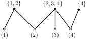
Figure 1: An exemple of tree in $\mathcal{T}_{4}$, with $\mathcal{I}(T)=\left\{\{1,2\},\{2,3,4\},\{4\}\right\}$.

A labeled bipartite tree $T$ (Fig. 1) is a bipartite tree whose white vertices are labeled from 1 to $p=\lvert W\rvert$. It can be encoded by a set $\mathcal{I}(T)$ whose elements are subsets $I\subset\{1,\ldots,p\}$ each representing a black vertex. If $b\in W$, the corresponding set is $I_{b}=\{i\in\{1,\ldots,p\}\mid(b,i)\in E\}$. The condition that $T$ is connected is equivalent to $\bigvee_{I\in\mathcal{I}(T)}\Pi(I)=1_{p}$, where $\Pi(I)$ is the partition of $\{1,\ldots,p\}$ obtained by supplementing $I$ by $1_{p-\lvert I\rvert}$. The condition that $T$ is a tree is translated to

$$\sum_{I\in\mathcal{I}(T)}(\lvert I\rvert-1)-p+1=0.$$ (2.6)

Note that this implies that if $I,J\in I\in\mathcal{I}(T)$, $\lvert I\cap J\rvert\leq 1$ (i.e. there are no multiple edges). For $i\in\{1,\ldots,p\}$, we denote by $\mathcal{I}_{i}(T)$ the subset of $\mathcal{I}(T)$ of sets containing $i$, and $\mathrm{deg}_{T}(i)=\lvert\mathcal{I}_{i}(T)\rvert$ the valency of the white vertex number $i$. It will be useful to introduce the notations $\mathcal{I}^{\prime}_{i}(T)$ and $\mathcal{I}^{\prime}(T)$ for the subsets of $\mathcal{I}_{i}(T)$ and $\mathcal{I}(T)$ which do no contain elements $I$ with only one element. The number of edges incident to the white vertex $i$ and whose other extremity is a black leaf is denoted by $\mathrm{deg}^{{\mathsf{L}}}_{T}(i)$. The number of edges of $T$ can be reformulated as $\lvert E(T)\rvert=\sum_{I\in\mathcal{I}(T)}\lvert I\rvert=\sum_{i=1}^{p}\mathrm{deg}_{T}(i)$. Note that the black leaves incident to a given white vertex $i$ of a labeled bipartite tree are not distinguishable, as they all correspond to the same $I=\{i\}$.

The set of labeled bipartite trees with $p$ white vertices is

$$\mathcal{T}_{p}=\biggl{\{}\mathcal{I}=\{I_{1},\ldots I_{k}\},k\geq 1,I_{a}\subset\{1,\ldots,p\}\mid\bigvee_{I\in\mathcal{I}}\Pi(I)=1_{p}\,;\,\sum_{I\in\mathcal{I}}(\lvert I\rvert-1)-p+1=0\biggr{\}},$$ (2.7)

and the subset of $\mathcal{T}_{p}$ of labeled trees for which all black vertices have valencies two or higher ($\forall I\in\mathcal{I}(T),\,|I\rvert\geq 2$) is denoted by $\mathcal{G}_{p}$. By convention, $\mathcal{G}_{1}$ has a single element, with one white vertex, no edge and no black vertex.

2.4 Bipartite maps

Two permutations $(\sigma_{1},\sigma_{2})\in S_{n}^{2}$ define a bipartite map. They bijectively encode a graph with $n$ labeled edges, embedded on a collection of $\#(\Pi(\sigma_{1})\vee\Pi(\sigma_{2}))$ surfaces, up to orientation preserving homeomorphisms. The genus $g=g(\sigma_{1},\sigma_{2})$ of that surface is given by the Euler characteristics

$$\#(\sigma_{1})+\#(\sigma_{2})+\#(\sigma_{1}\sigma_{2})-n=2\#(\Pi(\sigma_{1})\vee\Pi(\sigma_{2}))-2g(\sigma_{1},\sigma_{2}).$$ (2.8)

The graph is bipartite and the vertices of each kind - black or white - are respectively encoded by the disjoint cycles of $\sigma_{1}$ and $\sigma_{2}$, and the edges only link vertices of two different types. Each cycle of $\sigma_{i}$ is a cyclic sequence of numbers which corresponds to the labeled edges encountered cyclically when turning around one of the type $i$ vertices, counterclockwise. The number of vertices of each kind are respectively given by $\#(\sigma_{1})$ and $\#(\sigma_{2})$. Two consecutive edges around a vertex form a corner. The connected components of the complement of the graph on the surface - called faces - are therefore bijectively encoded by the disjoint cycles of $\sigma_{1}\sigma_{2}$, or equivalently of $\sigma_{2}\sigma_{1}$, so that in particular, $\#(\sigma_{1}\sigma_{2})=\#(\sigma_{2}\sigma_{1})$, and $g(\sigma_{1},\sigma_{2})=g(\sigma_{2},\sigma_{1})$. A bipartite map $(\sigma_{1},\sigma_{2})$ with $g(\sigma_{1},\sigma_{2})=0$ is planar.

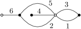
Figure 2: An exemple of (planar) bipartite map, with black vertices given by $\sigma_{1}=(13)(256)(4)$ and white vertices encoded by $\sigma_{2}=(13542)(6)$.

The Tutte dual is an operation which consists in adding a grey vertex in each face, and for each new vertex, an edge linking that vertex to each corner around a white vertex in the face it belongs to. This operation preserves the number of connected components and the genus, and the grey vertices are bijectively encoded by the disjoint cycles of $\sigma_{1}^{-1}\sigma_{2}^{-1}$ or $\sigma_{2}^{-1}\sigma_{1}^{-1}$. Said otherwise,

$$\#(\Pi(\sigma_{1})\vee\Pi(\sigma_{2}))=\#(\Pi(\sigma_{i})\vee\Pi(\sigma_{1}\sigma_{2}))=\#(\Pi(\sigma_{i})\vee\Pi(\sigma_{2}\sigma_{1})),$$ (2.9)

and

$$g(\sigma_{1},\sigma_{2})=g(\sigma_{i},\sigma_{1}^{-1}\sigma_{2}^{-1})=g(\sigma_{i},\sigma_{2}^{-1}\sigma_{1}^{-1}).$$ (2.10)

Finally, reversing the convention for the ordering of the edges from counterclockwise to clockwise obviously does not change the genus, so that $g(\sigma_{1},\sigma_{2})=g(\sigma_{1}^{-1},\sigma_{2}^{-1})$.

Consider a bipartite map $(\sigma,\tau)$, $\sigma,\tau\in S_{n}$, and one of its vertices (a cycle of either permutation), and two distinct corners around that vertex (two pairs of non-necessarily consecutive integers $a,b$ and $c,d$ in the cycle - $a,d$ on one hand and $b,c$ on the other are not necessarily distinct). The operation which consists in duplicating this vertex in two as shown in Fig. 3 is called splitting the vertex (along these two corners). It corresponds to composing from the left the corresponding permutation (e.g. $\sigma$) by the transposition $(d,b)$ (the new map is $(\sigma\circ(d,b),\tau)$). A cut-vertex can be split in a way that raises the number of connected components of the map.

                          

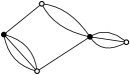
Figure 3: Left: splitting the vertex along two corners. Right: a non-separable hypermap.

A map for which there are no cut-vertices is usually called non-separable or 2-connected [23, 4, 5, 13, 15, 11]. A bipartite map which has no white cut-vertices will be called a non-separable hypermap.

It is known that any map has a unique decomposition in non-separable components (see e.g. [13]). This is also true for a non-separable hypermap, with a simple modification of the procedure: recursively split the white vertices along two corners whenever it raises the number of connected components until there are no such pairs of corners. The operation is commutative and the resulting terminal bipartite map uniquely defined. The connected components of the terminal bipartite map provide a unique decomposition of the original map in non-separable connected hypermaps. See the example in Fig. 4.

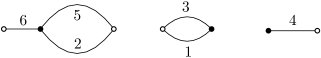
Figure 4: Decomposition of the bipartite map of Fig. 2 in non-separable hypermaps.

We stress that by Tutte duality (but linking the newly added grey vertices to the black vertices), non-separable hypermaps are dual to simple maps [1, 3, 2], yet not fully simple, and such that all faces are boundary faces. Splitting a white vertex then amounts to splitting a grey vertex, so that the decomposition in non-separable hypermaps corresponds to a decomposition is simple maps.

2.5 Constellations and Hurwitz numbers

We let for $\bar{\pi}\in\mathcal{P}(n)$ and $\nu\in S_{n}$ such that $\bar{\pi}\geq\Pi(\nu)$, and $l,k\in\mathbb{N}$:

$$M(\bar{\pi},\nu;l,k)=\mathrm{Card}\Bigl{\{}\rho_{1},\ldots,\rho_{k}\,\in\,S_{n}^{*}\ \mid\ \Pi(\hat{\rho})=\bar{\pi}\ ;\,\ \rho_{1}\cdots\;\rho_{k}=\nu\ ;\,\ \sum_{i=1}^{k}\lVert\rho_{i}\rVert=l\Bigr{\}}\;,$$ (2.11)

where $\Pi(\hat{\rho})=\bigvee_{i=1}^{k}\Pi(\rho_{i})$. The systems enumerated by $M$ are called $k$-constellations, and correspond to a specific kind of bipartite maps of genus $g$. The relation between $l$ and $g$ is then given by:

$$l=2g+n-2+\#(\nu).$$ (2.12)

If $\alpha\vdash n$ is a partition of $n$, we let $C_{\alpha}$ be the conjugacy class associated to $\alpha\vdash n$, whose cardinal is where $\lvert C_{\alpha}\rvert=n!/(\prod_{p\geq 1}p^{d_{p}(\alpha)}d_{p}(\alpha)!)$. For $\alpha\vdash n$ and $g\geq 0$, the genus-$g$ monotone Hurwitz number $\vec{H}_{g}(\alpha)$ is defined combinatorially by

$$\vec{H}_{g}(\alpha)=\lvert C_{\alpha}\rvert\times\mathrm{Card}\biggl{\{}\tau_{1},\ldots,\tau_{l}\mid\rho_{\alpha}=\tau_{1}\cdots\tau_{l}\ \ ;\ \bigvee_{1\leq i\leq l}\Pi(\tau_{i})=1_{n}\biggr{\}},$$

where $\rho_{\alpha}$ is any permutation in $C_{\alpha}$, and the $\tau_{i}$ are transpositions with weakly monotone maxima, that is, they can be written as $\tau_{i}=(p_{i}q_{i})$ where $\forall i,\ p_{i}<q_{i}$ and $q_{1}\leq\ldots\leq q_{l}$.

Divided by $n!$, $\vec{H}_{g}(\alpha)$ counts connected $n$-sheeted weighted ramified coverings of the 2-sphere by a surface of genus $g$, with $l+1$ ordered branch points, $l$ of which have simple ramification (they have $n-1$ preimages), the last point having ramification profile $\alpha$, where $l$ is given by (2.12). This relation is then called the Riemann-Hurwitz formula. The condition that the transpositions have weakly monotone maxima restricts the admissible coverings.

If $l\geq 0$ and $\nu\in S_{n}$, we define $\gamma_{l}(\nu)$ as

$$\gamma_{l}(\nu)=\sum_{k\geq 0}(-1)^{k}M(1_{n},\nu;l,k).$$ (2.13)

If $\nu\in C_{\alpha}$, $\gamma_{l}(\nu)$ can be related to $\vec{H}_{g}(\alpha)$ by [8, 16, 7]:

$$\gamma_{\#(\nu)+n+2g-2}(\nu)=\vec{H}_{g}(\alpha)\;\frac{(-1)^{\#(\nu)+n}}{\lvert C_{\alpha}\rvert}\;\;.$$ (2.14)

For $g=0$, from (2.12) $l=n-2+\#(\nu)$, and $\gamma(\nu):=\gamma_{\#(\nu)+n-2}(\nu)$, which is related to the genus 0 monotone Hurwitz number by

$$\gamma(\nu)=\vec{H}_{0}(\alpha)\;\frac{(-1)^{\#(\nu)+n}}{\lvert C_{\alpha}\rvert}\;\;.$$ (2.15)

This is computed explicitly as [6]:

$$\gamma(\nu)=(-1)^{\#(\nu)+n}\frac{(2n+\#(\nu)-3)!}{(2n)!}\prod_{p\geq 1}\left[\frac{(2p)!}{p!(p-1)!}\right]^{d_{p}(\nu)},$$ (2.16)

where $d_{p}(\nu)$ is the number of cycles of $\nu$ with $p$ elements.

More generally, we define for $l\geq 0$ and $\bar{\pi}\in\mathcal{P}(n)$ satisfying $\Pi(\nu)\leq\bar{\pi}<1_{n}$:

$$\gamma_{l}(\bar{\pi},\nu)=\sum_{k\geq 0}(-1)^{k}M(\bar{\pi},\nu;l,k).$$ (2.17)

Lemma 2.1 ([6], [7] Sec. 4.2).

It can be shown that:

$$\gamma_{l}(\bar{\pi},\nu)=\sum_{\begin{subarray}{c}\{l_{G}\}_{G\in\bar{\pi}}\geq 0\\ \sum_{G}l_{G}=l\end{subarray}}\;\prod_{G\in\bar{\pi}}\gamma_{l_{G}}({\nu}_{\lvert_{G}}).$$ (2.18)

Note that this implies that $(-1)^{\#(\nu)+n}\gamma_{l}(\bar{\pi},\nu)\geq 0$. For each $G$, (2.12) writes

$$l_{G}=2g_{G}+|G|-2+\#({\nu}_{\lvert_{G}}),$$ (2.19)

where $g_{G}$ is the genus of the constellations in the alternating sum, or of the coverings counted by the corresponding Hurwitz number. The proof is not succinct and we don’t repeat it here.

Lemma 2.2 ([7], Sec. 4.2).

Let $\bar{\pi},\tilde{\pi}\in\mathcal{P}(n)$ and $\nu\in S_{n}$. It is always true that if $\bar{\pi}\geq\Pi(\nu)$ and $\tilde{\pi}\geq\Pi(\nu)$:

$$L[\tilde{\pi},\bar{\pi};\Pi(\nu)]=\#(\nu)-\#(\tilde{\pi})-\#(\bar{\pi})+\#(\tilde{\pi}\vee\bar{\pi})\geq 0.$$ (2.20)

Furthermore, if $\pi,\tilde{\pi}$ such that $\pi\geq\tilde{\pi}\geq\Pi(\nu)$, there exists a $\bar{\pi}\geq\Pi(\nu)$ such that $\bar{\pi}\vee\tilde{\pi}=\pi$ and $L[\tilde{\pi},\bar{\pi};\Pi(\nu)]=0$.

Proof.

We construct an incidence graph $\mathcal{G}[\tilde{\pi},\bar{\pi};\Pi(\nu)]$ as follows (see Sec. 2.3). To each block of $\tilde{\pi}$ (resp. $\bar{\pi}$ ) we associate a black (resp. white) vertex. Each block of $\Pi(\nu)$ is contained both in a block of $\tilde{\pi}$ (corresponding to a black vertex) and a block of $\bar{\pi}$ (corresponding to a white vertex): for every block of $\Pi(\nu)$, we draw an edge between the corresponding black and white vertices (so that the graph is bipartite). The graph $\mathcal{G}[\tilde{\pi},\bar{\pi};\Pi(\nu)]$ has $\#(\tilde{\pi}\vee\bar{\pi})$ connected components, so that $L[\tilde{\pi},\bar{\pi};\Pi(\nu)]$ is its first Betti number (excess). The inequality is saturated if $\mathcal{G}[\tilde{\pi},\bar{\pi};\Pi(\nu)]$ is a forest. Showing the second assertion is equivalent to showing that given a collection of black vertices, each with a certain number of incident edges such that the other extremity of each edge is not connected to any vertex, it is always possible to group these free extremities to form new white vertices, so that the resulting graph is a tree. This of course is always true. ∎

The following is a slight generalization of the results of [6] and [7], Sec. 4.2.

Lemma 2.3.

We fix $\pi,\tilde{\pi}$ and $\nu$ such that $\pi\geq\tilde{\pi}\geq\Pi(\nu)$. The minimal value of $l$ such that

1. $\gamma_{l}(\bar{\pi},\nu)$ is non-vanishing

2. $\bar{\pi}$ satisfies $\pi\geq\bar{\pi}\geq\Pi(\nu)$ and $\tilde{\pi}\vee\bar{\pi}=\pi$,

is given by

$$\ell(\nu,\pi,\tilde{\pi})=n-\#(\nu)+2\bigl{(}\#(\tilde{\pi})-\#(\pi)\bigr{)}.$$ (2.21)

For this value to be reached, $\bar{\pi}$ must be such that

$$\#(\bar{\pi})=\#(\nu)-\#(\tilde{\pi})+\#(\pi),$$

which is always possible from the second point of Lemma 2.2. Furthermore,

$$\gamma_{\ell(\nu,\pi,\tilde{\pi})}(\bar{\pi},\nu)=\prod_{G\in\bar{\pi}}\gamma({\nu}_{\lvert_{G}}).$$ (2.22)

Proof.

Summing the relations (2.19) for the blocks of $\bar{\pi}$ in Lemma 2.1, we get:

$$l=2\sum_{G\in\bar{\pi}}g_{G}+n-2\#(\bar{\pi})+\#(\nu).$$ (2.23)

If $\nu$ is fixed, the minimal value of $l$ is reached for $\bar{\pi}=0_{n}$, but this is excluded if the condition $\tilde{\pi}\vee\bar{\pi}=\pi$ is imposed for $\tilde{\pi}<\pi$. Instead, we may rewrite (2.23) as:

$$l=\#(\nu)+2\bigl{(}\#(\tilde{\pi})-\#(\pi)\bigr{)}+2\sum_{G\in\bar{\pi}}g_{G}+2L[\tilde{\pi},\bar{\pi};\Pi(\nu)],$$ (2.24)

so that $l\geq\ell(\nu,\pi,\tilde{\pi})$, with equality if and only if $L[\tilde{\pi},\bar{\pi},\Pi(\nu)]=0$ and for all $G\in\bar{\pi}$, $g_{G}=0$. The second condition fixes all $l_{G}$ (2.19) to their minimal value $|G|-2+\#({\nu}_{\lvert_{G}})$, so that (2.18) simplifies to (2.22). ∎

2.6 Higher order free cumulants

2.6.1 Finite $N$

Higher order free cumulants were introduced in [9]. As in Notation 4.1 p. 20 of this reference, we define for $\pi\geq\Pi(\tau)$, $\pi\in\mathcal{P}(n)$, $\tau\in S_{n}$, and $\vec{B}=(B_{1},\ldots,B_{n})$:

$$\varphi(\pi,\tau)[\vec{B}]=\prod_{G\in\pi}k_{\#(\tau\lvert_{{}_{G}})}\biggl{(}\Bigl{\{}{\mathrm{Tr}}\Bigl{(}\vec{\prod}_{j\in\tau_{i}}B_{j}\Bigr{)}\Bigr{\}}_{\tau_{i}\textrm{ cycle of }\tau\lvert_{{}_{G}}}\biggr{)},$$ (2.25)

where the classical cumulants $k_{n}$ have been introduced in Sec. 2.2. For $\vec{B}=(B,\ldots,B)$ (in which case we remove the arrow), this relation simplifies to:

$$\varphi(\pi,\tau)[B]=\prod_{G\in\pi}k_{\#(\tau\lvert_{{}_{G}})}\biggl{(}\Bigl{\{}{\mathrm{Tr}}\bigl{(}B^{\lvert V\rvert}\bigr{)}\Bigr{\}}_{V\in\Pi(\tau_{\lvert_{{}_{G}}})}\biggr{)}.$$ (2.26)

The following are then defined for $\sigma\in S_{n}$ (eq (24) and (14) in [9]):

$$\kappa(\pi,\sigma)[\vec{B}]=\sum_{\tau\in S_{n}}\sum_{\begin{subarray}{c}{\pi^{\prime}\in\mathcal{P}(n)}\\ {\pi\geq\pi^{\prime}\geq\Pi(\tau)}\end{subarray}}\varphi(\pi^{\prime},\tau)[\vec{B}]\sum_{\begin{subarray}{c}{\pi^{\prime\prime}\in\mathcal{P}(n)}\\ {\pi\geq\pi^{\prime\prime}\geq\Pi(\sigma)\vee\pi^{\prime}}\end{subarray}}\lambda_{\pi^{\prime\prime},\pi}\prod_{G\in\pi^{\prime\prime}}W^{(N)}\Bigl{(}\left(\sigma\tau^{-1}\right)_{\lvert_{{}_{G}}}\Bigr{)},$$ (2.27)

where the $W^{(N)}$ are the Weingarten functions, which can be shown (see [10]) to have the expansion:

$$W^{(N)}(\nu)=N^{-n}\sum_{k\geq 0}\;\sum_{\begin{subarray}{c}{\rho_{1},\ldots,\rho_{k}\,\in\,S_{n}^{*},}\\ {\rho_{1}\cdots\rho_{k}=\nu}\end{subarray}}\;(-1)^{k}\,N^{-\sum_{i=1}^{k}\lVert\rho_{i}\rVert}\;,$$ (2.28)

which can be written using (2.17) as:

$$W^{(N)}(\nu)=\sum_{\begin{subarray}{c}\pi\in\mathcal{P}(n)\\ \pi\geq\Pi(\nu)\end{subarray}}\sum_{l\geq 0}\,N^{-n-l}\;\gamma_{l}(\pi,\nu).$$ (2.29)

Note that (2.27) is well-defined, because since $\pi^{\prime}\geq\Pi(\tau)=\Pi(\tau^{-1})$, from (2.9): $\Pi(\sigma)\vee\pi^{\prime}=\Pi(\sigma)\vee\Pi(\tau^{-1})\vee\pi^{\prime}=\Pi(\sigma)\vee\Pi(\sigma\tau^{-1})\vee\pi^{\prime}\geq\Pi(\sigma\tau^{-1})$, so that $\pi^{\prime\prime}\geq\Pi(\sigma\tau^{-1})$.

The inverse relation of (2.27) is given in [9]:

$$\varphi(\pi,\sigma)[\vec{B}]=\sum_{\begin{subarray}{c}{\tau\in S_{n},\,\pi^{\prime}\in\mathcal{P}(n)}\\[0.60275pt] {\pi\geq\pi^{\prime}\geq\Pi(\tau)}\\ {\pi^{\prime}\vee\Pi(\sigma\tau^{-1})=\pi}\end{subarray}}\kappa(\pi^{\prime},\tau)[\vec{B}]\,\cdot\,N^{\#(\sigma\tau^{-1})}.$$ (2.30)

2.6.2 Asymptotics

From [9], $\varphi(\pi,\sigma)[\vec{B}]$ is of order $N^{2\#(\pi)-\#(\sigma)}$, so that we define

$$\varphi(\pi,\sigma)[\vec{b}]=\lim_{N\rightarrow\infty}N^{\#(\sigma)-2\#(\pi)}\varphi(\pi,\sigma)[\vec{B}],$$ (2.31)

and $\kappa(\pi,\sigma)[\vec{B}]$ is of order $N^{2\#(\pi)-n-\#(\sigma)}$. Defining the higher order free cumulants by

$$\kappa(\pi,\sigma)[\vec{b}]=\lim_{N\rightarrow\infty}N^{\#(\sigma)+n-2\#(\pi)}\kappa(\pi,\sigma)[\vec{B}],$$ (2.32)

the asymptotics of (2.30) are derived in [9]. We describe them below.

Proposition 2.4 ([9]).

For $\pi\in\mathcal{P}(n)$ and $\sigma\in S_{n}$ satisfying $\pi\geq\Pi(\sigma)$,

$$\varphi(\pi,\sigma)[\vec{b}]=\sum_{\begin{subarray}{c}{\tau\in S_{n},\,\pi^{\prime}\in\mathcal{P}(n)}\\[0.60275pt] {\pi\geq\pi^{\prime}\geq\Pi(\tau)}\\ {\pi^{\prime}\vee\Pi(\sigma\tau^{-1})=\pi}\\ {\#(\tau)-2\#(\pi^{\prime})-\#(\sigma\tau^{-1})+n=\#(\sigma)-2\#(\pi)}\end{subarray}}\kappa(\pi^{\prime},\tau)[\vec{b}].$$ (2.33)

This is rewritten through the use of a dot-product (see Def. 4.9 and Notation 4.6 of [9])

$$(\pi_{1},\sigma_{1})\cdot(\pi_{2},\sigma_{2})=(\pi,\sigma)\Leftrightarrow\left\{\begin{array}[]{lll}\pi=\pi_{1}\vee\pi_{2}\\ \sigma=\sigma_{1}\sigma_{2}\\ \#(\sigma_{1})-2\#(\pi_{1})+\#(\sigma_{2})-2\#(\pi_{2})+n=\#(\sigma)-2\#(\pi)\end{array}\right.,$$ (2.34)

so that:

$$\varphi(\pi,\sigma)[\vec{b}]=\sum_{\begin{subarray}{c}{\tau\in S_{n},\,\pi^{\prime}\in\mathcal{P}(n)}\\[0.60275pt] {\pi^{\prime}\geq\Pi(\tau)}\\[0.60275pt] {(\pi^{\prime},\tau)\cdot(\Pi(\sigma\tau^{-1}),\;\sigma\tau^{-1})=(\pi,\sigma)}\end{subarray}}\kappa(\pi^{\prime},\tau)[\vec{b}].$$ (2.35)

A function $f:\pi\geq\sigma\rightarrow f(\pi,\sigma)$ is said to be multiplicative if $f(\pi,\sigma)=\prod_{G\in\pi}f(1_{{\lvert G\rvert}},\sigma_{\mid{{}_{\lvert G\rvert}}})$, and $f(1_{n},\sigma)$ depends only on $\Lambda(\sigma)$. in the sense that for all $\nu\in S_{n}$ and denoting by $\vec{b}_{\nu}=(b_{\nu(1)},\ldots,b_{\nu(n)})$ whereas $\vec{b}=(b_{1},\ldots,b_{n})$:

$$\varphi(1_{n},\nu^{-1}\sigma\nu)[\vec{b}_{\nu}]=f(1_{n},\sigma)[\vec{b}],$$ (2.36)

and similarly for $\kappa$. Both $\varphi(\pi,\sigma)[\vec{b}]$ and $\kappa(\pi,\sigma)[\vec{b}]$ are multiplicative functions. Given $\pi,\tau$, $\pi\geq\Pi(\tau)$, and two multiplicative functions $f$ and $g$, their convolution is defined as:

$$(f\star g)(\pi,\sigma)=\sum_{\begin{subarray}{c}{\sigma_{1},\sigma_{2}\in S_{n},\ \pi_{1},\pi_{2}\in\mathcal{P}(n)}\\[0.60275pt] {\pi_{1}\geq\Pi(\sigma_{1}),\ \pi_{2}\geq\Pi(\sigma_{2})}\\[0.60275pt] {(\pi_{1},\sigma_{1})\cdot(\pi_{2},\sigma_{2})=(\pi,\sigma)}\end{subarray}}f(\pi_{1},\sigma_{1})g(\pi_{2},\sigma_{2}).$$ (2.37)

The relations (2.33) and (2.35) can in turn be expressed as

$$\varphi(\pi,\sigma)[\vec{b}]=(f\star\zeta)(\pi,\sigma),$$ (2.38)

where $f:\pi\geq\sigma\rightarrow\kappa(\pi,\sigma)[\vec{b}]$ and $\zeta:\pi\geq\sigma\rightarrow\delta_{\pi,\Pi(\sigma)}$. From the multiplicativity and the rules of this convolution, (2.38) and thereby (2.33) can be inverted, yielding (see Def 7.4 of [9]):

Theorem 2.5 ([9]).

For $\pi\in\mathcal{P}(n)$ and $\sigma\in S_{n}$ satisfying $\pi\geq\Pi(\sigma)$,

$$\kappa(\pi,\sigma)[\vec{b}]=\sum_{\begin{subarray}{c}{\sigma_{1},\sigma_{2}\in S_{n},\ \pi_{1},\pi_{2}\in\mathcal{P}(n)}\\[0.60275pt] {\pi_{1}\geq\Pi(\sigma_{1}),\ \pi_{2}\geq\Pi(\sigma_{2})}\\[0.60275pt] {(\pi_{1},\sigma_{1})\cdot(\pi_{2},\sigma_{2})=(\pi,\sigma)}\end{subarray}}\varphi(\pi_{1},\sigma_{1})[\vec{b}]\,\,\mu(\pi_{2},\sigma_{2}),$$ (2.39)

where $\mu$ is given as a series by

$$\mu(\pi_{2},\sigma_{2})=\delta(\pi_{2},0_{n})\delta(\sigma_{2},\mathrm{id})+\sum_{k\geq 0}\,(-1)^{k}\sum_{\begin{subarray}{c}{\rho_{1},\ldots,\rho_{k}\in S_{n}^{*}}\\ {(\pi_{2},\sigma_{2})=(\Pi(\rho_{1}),\rho_{1})\cdot\ldots\cdot(\Pi(\rho_{k}),\rho_{k})}\end{subarray}}1,$$ (2.40)

where the $\delta$ function are Kronecker functions.

More explicitly:

$$\kappa(\pi,\sigma)[\vec{b}]=\sum_{\begin{subarray}{c}{\sigma_{1},\sigma_{2}\in S_{n},\ \pi_{1},\pi_{2}\in\mathcal{P}(n)}\\[0.3014pt] {\pi_{1}\geq\Pi(\sigma_{1}),\ \pi_{2}\geq\Pi(\sigma_{2})}\\[1.50694pt] {\pi_{1}\vee\pi_{2}=\pi,\ \sigma_{1}\sigma_{2}=\sigma}\\[1.20552pt] {\#(\sigma_{1})-2\#(\pi_{1})+\#(\sigma_{2})-2\#(\pi_{2})+n=\#(\sigma)-2\#(\pi)}\end{subarray}}\varphi(\pi_{1},\sigma_{1})[\vec{b}]\ \,\,\mu(\pi_{2},\sigma_{2}).$$ (2.41)

Whereas this result is obtained in [9] using the properties of the convolution to invert (2.38), we will reformulate (2.39) in Sec. 3.1 as a tree-like sum involving only one partition and one permutation instead of two each, and show that this simpler expression can be derived directly by taking the asymptotics of (2.27) using the properties of the Weingarten functions (Sec. 3.2).

Assuming that $\vec{b}=(b,\ldots,b)$, the higher order moments and cumulants only depend on the partition $\lambda=\Lambda(\sigma)=(\lambda_{1},\ldots,\lambda_{p})\vdash n$ of the permutation $\sigma\in S_{n}$ (see (2.26)), that is, for any $\sigma\in C_{\lambda}$, where $\#(\lambda)=p$:

$$\varphi_{p}(\lambda)[b]:=\varphi(1_{n},\sigma)[b]=\lim_{N\rightarrow\infty}N^{p-2}k_{p}\Bigl{(}\bigl{\{}{\mathrm{Tr}}(B^{\lambda_{i}})\bigr{\}}_{1\leq i\leq p}\Bigr{)}.$$

The following notation is also common:

$$\varphi_{p}(b^{\lambda_{1}},\ldots,b^{\lambda_{p}})=\varphi_{p}(\lambda)[b].$$ (2.42)

In the same way, for any $\sigma\in C_{\lambda}$, where $\#(\lambda)=p$:

$$\kappa(\lambda)[b]:=\kappa(1_{n},\sigma)[b]=\kappa(1_{n},\gamma_{\lambda_{1},\ldots,\lambda_{p}})[b],$$ (2.43)

where $\gamma$ was defined in (2.1). We use the following notation for the higher order free cumulants:

$$\kappa_{\lambda_{1},\ldots,\lambda_{p}}[b]=\kappa_{\{\lambda_{i}\}}[b]=\kappa(\lambda)[b].$$ (2.44)

The free cumulants (of first order) are obtained for $\lambda$ the one-part partition ($p=1$) and are denoted by

$$\kappa_{n}[b]:=\kappa(1_{n},\gamma_{n})[b].$$ (2.45)

2.6.3 Resolution

The following reformulation of (2.35) has been derived in [24] for $p=\#(\lambda)=1$, in [9] for $p=2$, and in [2] for $p\geq 3$ (Thm. 3.12). These combinatorial relations correspond - coefficientwise - to the analytic functional relations between the generating series of higher order moments and cumulants (we do not repeat the functional relations here in full generality). We recall that $\mathcal{G}_{p}$ is the set of bipartite trees with $p$ labeled white vertices and no black leaves, and define the following generating functions:

$$M_{2}(X_{1},X_{2})=\sum_{a_{1},a_{2}\geq 1}\varphi_{2}(b^{a_{1}},b^{a_{2}})X_{1}^{a_{1}}X_{2}^{a_{2}},\qquad\mathrm{and}\qquad C_{2}(Y_{1},Y_{2})=\sum_{a_{1},a_{2}\geq 1}\kappa_{a_{1},a_{2}}[b]\ Y_{1}^{a_{1}}Y_{2}^{a_{2}}.$$ (2.46)

Theorem 2.6 ([24, 9, 2]).

For $p\geq 1$ and $\lambda\vdash n$, $n\geq 1$,

$$\tilde{\varphi}_{p}(b^{\lambda_{1}},\ldots,b^{\lambda_{p}})=\sum_{T\in\mathcal{G}_{p}}\sum_{i=1}^{p}\sum_{l_{i}\geq 1}\sum_{\begin{subarray}{c}{\{j^{I}_{i}\geq 1\}_{I\in\mathcal{I}_{i}(T)}}\\ {\{m_{i}^{(s)}\geq 1\}_{1\leq s\leq l_{i}}}\\[1.50694pt] {\sum_{I\in\mathcal{I}_{i}(T)}j^{I}_{i}+\sum_{s=1}^{l_{i}}m_{i}^{(s)}=\lambda_{i}}\end{subarray}}\left(\prod^{\prime}_{I\in\mathcal{I}(T)}\kappa_{\{j_{i}^{I}\}_{i\in I}}[b]\right)$$

$$\hskip 199.16928pt\times\left(\prod_{i=1}^{p}\frac{\lambda_{i}!}{l_{i}!(\lambda_{i}+1-l_{i}-\mathrm{deg}_{T}(i))!}\prod_{s=1}^{l_{i}}\kappa_{m_{i}^{(s)}}[b]\right),$$

where $\mathcal{I}_{i}(T)=\{I\in\mathcal{I}(T),i\in I\}$, $\mathrm{deg}_{T}(i)=\lvert\mathcal{I}_{i}(T)\rvert$ is the valency of the $i$th white vertex of $T$, and $\prod^{\prime}$ means that if $\lvert I\rvert=2$, $\kappa_{j_{1},j_{2}}[b]$ should be replaced with

$$\kappa_{j_{1},j_{2}}[b]\quad\rightarrow\quad\alpha_{j_{1},j_{2}}[b]=\langle Y_{1}^{j_{1}}\rangle\langle Y_{2}^{j_{2}}\rangle\Biggl{\{}C_{2}(Y_{1},Y_{2})+\frac{Y_{1}Y_{2}}{(Y_{1}-Y_{2})^{2}}\Biggr{\}},$$ (2.47)

and $\tilde{\varphi}_{p}$ is $\varphi_{p}$ for $p\neq 2$, and

$$\tilde{\varphi}_{2}(b^{\lambda_{1}},b^{\lambda_{2}})=\langle X_{1}^{\lambda_{1}}\rangle\langle X_{2}^{\lambda_{2}}\rangle\Biggl{\{}M_{2}(X_{1},X_{2})+\frac{X_{1}X_{2}}{(X_{1}-X_{2})^{2}}\Biggr{\}}.$$ (2.48)

Immediate reformulations.

Each sum over the variables $m_{i}^{(s)}$ can be traded for a sum over $k_{1}^{(i)},\ldots,k_{\lambda_{i}}^{(i)}$ for the cost of a multinomial $(\sum_{a}k_{a}^{(i)})!/\prod_{a}k_{a}^{i}!$, with $l_{i}=\sum_{a=1}^{\lambda_{i}}k_{a}^{(i)}$:

$$\varphi_{p}(b^{\lambda_{1}},\ldots,b^{\lambda_{p}})=\sum_{T\in\mathcal{G}_{p}}\sum_{i=1}^{p}\sum_{l_{i}\geq 1}\sum_{\begin{subarray}{c}{\{j^{I}_{i}\geq 1\}_{I\in\mathcal{I}_{i}(T)}}\\ {k_{1}^{(i)},\ldots,k^{(i)}_{\lambda_{i}}\geq 0,\,\,\sum_{a=1}^{\lambda_{i}}k_{a}^{(i)}=l_{i}}\\[1.50694pt] {\sum_{I\in\mathcal{I}_{i}(T)}j^{I}_{i}+\sum_{a=1}^{\lambda_{i}}ak_{a}^{(i)}=\lambda_{i}}\end{subarray}}\left(\prod^{\prime}_{I\in\mathcal{I}(T)}\kappa_{\{j_{i}^{I}\}_{i\in I}}[b]\right)$$ (2.49)

$$\hskip 199.16928pt\times\left(\prod_{i=1}^{p}\frac{\lambda_{i}!}{(\lambda_{i}+1-l_{i}-\mathrm{deg}_{T}(i))!}\prod_{a=1}^{\lambda_{i}}\frac{1}{k_{a}^{(i)}!}\,\kappa_{a}[b]^{k_{a}^{(i)}}\right).$$

We may sum over $T^{\prime}\in\mathcal{T}_{p}$ instead of $T\in\mathcal{G}_{p}$, by adding $l_{i}$ black leaves to the vertex $i$. For $T^{\prime}$, $\mathrm{deg}_{T}(i)$ is the number of edges not incident to leaves in $T^{\prime}$, $l_{i}=\mathrm{deg}^{\mathsf{L}}_{T^{\prime}}(i)$, so that $l_{i}+\mathrm{deg}_{T}(i)=\mathrm{deg}_{T^{\prime}}(i)$. Some weights have been assigned to the edges of the tree:

• the edges incident to black vertices of valency larger than one are identified by a pair $(i,I)$, $1\leq i\leq p$, $I\in\mathcal{I}^{\prime}(T)$, and have been assigned a weight $j_{i}^{I}$,

• the black leaves incident to the white vertex $i\in\{1,\ldots,p\}$ are undistinguishable, so to each white vertex $i$ is associated an unordered list of weights, that is, a list $\{k_{a}^{(i)}\}_{1\leq a\leq\lambda_{i}}$, where $k_{a}^{(i)}$ is the number of black leaves associated to the white vertex $i$ that have a weight equal to $a$.

The formula of the theorem may therefore be re-stated as follows:

$$\varphi_{p}(b^{\lambda_{1}},\ldots,b^{\lambda_{p}})=\sum_{\begin{subarray}{c}{T\in\mathcal{T}_{p}}\\ {\forall i,\deg_{T}^{\mathsf{L}}(i)\geq 1}\end{subarray}}\prod_{i=1}^{p}\frac{\lambda_{i}!}{(\lambda_{i}+1-\mathrm{deg}_{T}(i))!}\sum_{i=1}^{p}\sum_{\begin{subarray}{c}{\{j^{I}_{i}\geq 1\}_{I\in\mathcal{I}_{i}(T)}}\\[1.50694pt] {\sum_{I\in\mathcal{I}_{i}(T)}j^{I}_{i}=\lambda_{i}}\end{subarray}}\prod^{\prime}_{I\in\mathcal{I}(T)}\kappa_{\{j_{i}^{I}\}_{i\in I}}[b]\prod_{i=1}^{p}\prod_{a=1}^{\lambda_{i}}\frac{1}{k_{a}^{(i)}!},$$ (2.50)

where as discussed above, the weights $j_{i}^{\{i\}}$ are an unordered list of $\mathrm{deg}_{T}^{\mathsf{L}}(i)$ positive integers, and $k_{a}^{(i)}$ is the number of these weights equal to $a$.

First order.

For $p=1$, we use the formulation (2.49) of the theorem. $\lambda$ has one block $\lambda_{1}=n$. The convention is that a tree with one white vertex but no leaves is just a single vertex (so that $\mathcal{I}(T)$ is empty). Thus, (2.49) simplifies to:

$$\varphi_{1}(b^{n})=\sum_{l=1}^{n}\sum_{\begin{subarray}{c}{\{k_{i}\geq 0\}_{1\leq i\leq n}}\\[0.60275pt] {\sum_{i=1}^{n}k_{i}=l}\\[0.60275pt] {\sum_{i=1}^{n}ik_{i}=n}\end{subarray}}\frac{n!}{(n+1-l)!}\prod_{i=1}^{n}\frac{\kappa_{i}[b]^{k_{i}}}{k_{i}!}=\sum_{\begin{subarray}{c}{\{k_{i}\geq 0\}_{1\leq i\leq n}}\\[0.60275pt] {\sum_{i=1}^{n}ik_{i}=n}\end{subarray}}\frac{n!}{\prod_{i}k_{i}!(n+1-\sum_{i=1}^{n}k_{i})!}\prod_{i=1}^{n}\kappa_{i}[b]^{k_{i}},$$ (2.51)

which as detailed in Corollary 2.6 of [24] or Corollary 1 of [22] is a combinatorial reformulation of the relation between generating functions

$$C_{1}(XM_{1}(X))=M_{1}(X),$$ (2.52)

where

$$M_{1}(X)=1+\sum_{a\geq 1}\varphi_{1}(b^{a})X^{a},\qquad\mathrm{and}\qquad C_{1}(Y)=1+\sum_{a\geq 1}\kappa_{a}[b]Y^{a}.$$ (2.53)

Second order.

For $p=2$, there is a single tree in $\mathcal{G}_{2}$, with two white vertices and one black vertex of valency two ($\mathcal{I}$ consists of a single set $\{1,2\}$). Theorem 2.6 simplifies to:

$$\tilde{\varphi}_{2}(b^{\lambda_{1}},b^{\lambda_{2}})=\sum_{\begin{subarray}{c}{j_{1},j_{2}\geq 1}\end{subarray}}\alpha_{j_{1},j_{2}}[b]\ \prod_{i=1}^{2}\Biggl{(}\sum_{l_{i}\geq 1}\binom{\lambda_{i}}{l_{i}}\sum_{\begin{subarray}{c}{\{m_{i}^{(s)}\geq 1\}_{1\leq s\leq l_{i}}}\\[1.50694pt] {\sum_{s=1}^{l_{i}}m_{i}^{(s)}=\lambda_{i}-j_{i}}\end{subarray}}\prod_{s=1}^{l_{i}}\kappa_{m_{i}^{(s)}}[b]\Biggr{)}.$$ (2.54)

To carry out the sums on the right hand side, we notice that since $\lambda>j$ (as $s\geq 1$):

$$\sum_{l\geq 1}\binom{\lambda}{l}\sum_{\begin{subarray}{c}{\{m^{(s)}\geq 1\}_{1\leq s\leq l}}\\[1.50694pt] {\sum_{s=1}^{l}m^{(s)}=\lambda-j}\end{subarray}}\prod_{s=1}^{l}\kappa_{m^{(s)}}[b]=\sum_{l=1}^{\lambda-j}\binom{\lambda}{l}\langle z^{\lambda-j}\rangle\biggl{(}\sum_{a=1}^{\lambda-j}\kappa_{a}[b]z^{a}\biggr{)}^{l}=\langle z^{\lambda-j}\rangle\biggl{(}1+\sum_{a=1}^{\lambda-j}\kappa_{a}[b]z^{a}\biggr{)}^{\lambda},$$ (2.55)

where $\langle z^{n}\rangle(\sum_{a\geq 0}c_{a}z^{a})=c_{n}$. By Lagrange inversion (see [12], Eq. (2.2.1)):

$$\langle z^{\lambda-j}\rangle\biggl{(}1+\sum_{a\geq 1}\kappa_{a}[b]z^{a}\biggr{)}^{\lambda-K}=\frac{\lambda-K}{j-K}\ \langle t^{\lambda-K}\rangle\biggl{(}t+\sum_{a\geq 1}\varphi_{1}(b^{a})t^{a+1}\biggr{)}^{j-K},$$ (2.56)

so that (here $K=0$):

$$\tilde{\varphi}_{2}(b^{\lambda_{1}},b^{\lambda_{2}})=\sum_{\begin{subarray}{c}{j_{1},j_{2}\geq 1}\end{subarray}}\alpha_{j_{1},j_{2}}[b]\ \prod_{i=1}^{2}\Biggl{(}\frac{\lambda_{i}}{j_{i}}\sum_{\begin{subarray}{c}{n_{i}^{(1)},\ldots,n_{i}^{(j_{i})}\geq 0}\\ {\sum_{s=1}^{j_{i}}n_{i}^{(s)}=\lambda_{i}-j_{i}}\end{subarray}}\prod_{s=1}^{j_{i}}\varphi_{1}(b^{n_{i}^{(s)}})\Biggr{)},$$ (2.57)

with the convention that $\varphi_{1}(b^{0})=1$. Noticing that

$$j\sum_{\begin{subarray}{c}{\{n^{(s)}\geq 0\}_{1\leq s\leq j}}\\[1.50694pt] {\sum_{s=1}^{j}n^{(s)}=P}\end{subarray}}n^{(1)}\prod_{s=1}^{j}\varphi_{1}\Bigl{(}b^{n^{(s)}}\Bigr{)}=\sum_{s=1}^{j}\sum_{\begin{subarray}{c}{\{n^{(s)}\geq 0\}_{1\leq s\leq j}}\\[1.50694pt] {\sum_{s=1}^{j}n^{(s)}=P}\end{subarray}}n^{(s)}\prod_{s=1}^{j}\varphi_{1}\Bigl{(}b^{n^{(s)}}\Bigr{)}=P\sum_{\begin{subarray}{c}{\{n^{(s)}\geq 0\}_{1\leq s\leq j}}\\[1.50694pt] {\sum_{s=1}^{j}n^{(s)}=\lambda-j}\end{subarray}}\prod_{s=1}^{j}\varphi_{1}(b^{n^{(s)}}),$$ (2.58)

where $P=\lambda-j$, we obtain the following:

$$\tilde{\varphi}_{2}(b^{\lambda_{1}},b^{\lambda_{2}})=\sum_{\begin{subarray}{c}{j_{1},j_{2}\geq 1}\end{subarray}}\alpha_{j_{1},j_{2}}[b]\ \prod_{i=1}^{2}\Biggl{(}\sum_{\begin{subarray}{c}{\{n_{i}^{(s)}\geq 0\}_{1\leq s\leq j_{i}}}\\[1.50694pt] {\sum_{s=1}^{j_{i}}n_{i}^{(s)}=\lambda_{i}-j_{i}}\end{subarray}}(1+n_{i}^{(1)})\prod_{s=1}^{j_{i}}\varphi_{1}\Bigl{(}b^{n_{i}^{(s)}}\Bigr{)}\Biggr{)},$$ (2.59)

which is to be compared with the key combinatorial reformulation of (2.33) derived in Prop. 6.2 of [9]. Going to generating functions, we indeed recover from (2.59) the second order functional relations

$$M_{2}(X_{1},X_{2})+\frac{X_{1}X_{2}}{(X_{1}-X_{2})^{2}}=\frac{\mathrm{d}\ln Y_{1}}{\mathrm{d}\ln X_{1}}\frac{\mathrm{d}\ln Y_{2}}{\mathrm{d}\ln X_{2}}\left(C_{2}(Y_{1},Y_{2})+\frac{Y_{1}Y_{2}}{(Y_{1}-Y_{2})^{2}}\right),$$ (2.60)

where $M_{1}$ has been defined in (2.52), $M_{2}$ and $C_{2}$ in (2.46), and

$$Y_{i}=X_{i}M_{1}(X_{i}),\qquad\mathrm{and}\qquad\frac{\mathrm{d}\ln Y_{i}}{\mathrm{d}\ln X_{i}}=\frac{\frac{\mathrm{d}}{\mathrm{d}X_{i}}Y_{i}}{M_{1}(X_{i})}.$$ (2.61)

For $n\geq 3$, the formulas are derived through Fock space methods, and deriving a combinatorial proof is still open (see the discussion page 24 of [2]).

2.6.4 Simpler formulation of the generating functions formulas

In view of the computations carried above for $p=2$, we may reformulate Thm. 2.6 as follows.

$$\varphi_{p}(b^{\lambda_{1}},\ldots,b^{\lambda_{p}})=\sum_{T\in\mathcal{G}_{p}}\ \sum_{\{j^{I}_{i}\geq 1\}_{\begin{subarray}{c}{1\leq i\leq p}\\ {I\in\mathcal{I}_{i}(T)}\end{subarray}}}\left(\prod^{\prime}_{I\in\mathcal{I}(T)}\kappa_{\{j_{i}^{I}\}_{i\in I}}[b]\right)$$ (2.62)

$$\hskip 113.81102pt\times\prod_{i=1}^{p}\frac{\lambda_{i}!}{(\lambda_{i}+1-\mathrm{deg}_{T}(i))!}\langle z^{\lambda_{i}-\sum_{I\in\mathcal{I}_{i}(T)}j_{i}^{I}}\rangle\biggl{(}1+\sum_{a\geq 1}\kappa_{a}[b]z^{a}\biggr{)}^{\lambda_{i}+1-\mathrm{deg}_{T}(i)}.$$

By Lagrange inversion again ((2.56) for $K=\mathrm{deg}_{T}(i)-1$), and then using (2.58) with $J_{i}-\mathrm{deg}_{T}(i)+1$ instead of $j$, where $J_{i}=\sum_{I\in\mathcal{I}_{i}(T)}j_{i}^{I}$ and with $P=\lambda_{i}-J_{i}$, we obtain the generalization for arbitrary $p\geq 2$ of the expression analogous to (2.59) for $p=2$:

$$\varphi_{p}(b^{\lambda_{1}},\ldots,b^{\lambda_{p}})=\sum_{T\in\mathcal{G}_{p}}\ \sum_{\{j^{I}_{i}\geq 1\}_{\begin{subarray}{c}{1\leq i\leq p}\\ {I\in\mathcal{I}_{i}(T)}\end{subarray}}}\left(\prod^{\prime}_{I\in\mathcal{I}(T)}\kappa_{\{j_{i}^{I}\}_{i\in I}}[b]\right)$$ (2.63)

$$\hskip 85.35826pt\times\prod_{i=1}^{p}\frac{\lambda_{i}!}{(\lambda_{i}+1-\mathrm{deg}_{T}(i))!}\sum_{\begin{subarray}{c}{\{n_{i}^{(s)}\geq 0\}_{1\leq s\leq J_{i}-\mathrm{deg}_{T}(i)+1}}\\[1.50694pt] {\sum_{s=1}^{J_{i}}n_{i}^{(s)}=\lambda_{i}-J_{i}}\end{subarray}}(1+n_{i}^{(1)})\prod_{s=1}^{J_{i}-\mathrm{deg}_{T}(i)+1}\varphi_{1}\Bigl{(}b^{n_{i}^{(s)}}\Bigr{)},$$

with the convention that $\varphi_{1}(b^{0})=1$. Noticing that:

$$\sum_{\begin{subarray}{c}{\{n^{(s)}\geq 0\}_{1\leq s\leq J-K}}\\[1.50694pt] {\sum_{s=1}^{J}n^{(s)}=\lambda-J}\end{subarray}}(1+n^{(1)})\prod_{s=1}^{J-K}\varphi_{1}\Bigl{(}b^{n^{(s)}}\Bigr{)} =\langle X^{\lambda-K}\rangle\ X\frac{\mathrm{d}}{\mathrm{d}X}\bigl{(}XM_{1}(X)\bigr{)}\bigl{(}XM_{1}(X)\bigr{)}^{J-K-1}$$ (2.64)

$$=\langle X^{\lambda}\rangle\ \frac{1}{M_{1}(X)^{K+1}}\frac{\mathrm{d}}{\mathrm{d}X}\bigl{(}XM_{1}(X)\bigr{)}\bigl{(}XM_{1}(X)\bigr{)}^{J},$$ (2.65)

and that

$$\frac{\lambda!}{(\lambda-K)!}\langle X^{\lambda}\rangle f(X)=\langle X^{\lambda-K}\rangle\frac{\mathrm{d}^{K}}{\mathrm{d}X^{K}}f(X)=\langle X^{\lambda}\rangle X^{K}\frac{\mathrm{d}^{K}}{\mathrm{d}X^{K}}f(X),$$ (2.66)

we may write:

$$\varphi_{p}(b^{\lambda_{1}},\ldots,b^{\lambda_{p}})=\biggl{(}\prod_{i=1}^{p}\langle X_{i}^{\lambda_{i}}\rangle\biggr{)}\sum_{T\in\mathcal{G}_{p}}\ \sum_{\{j^{I}_{i}\geq 1\}_{\begin{subarray}{c}{1\leq i\leq p}\\ {I\in\mathcal{I}_{i}(T)}\end{subarray}}}\left(\prod^{\prime}_{I\in\mathcal{I}(T)}\kappa_{\{j_{i}^{I}\}_{i\in I}}[b]\right)$$ (2.67)

$$\hskip 113.81102pt\times\left(\prod_{i=1}^{p}X_{i}^{\mathrm{deg}_{T}(i)-1}\frac{\mathrm{d}^{\mathrm{deg}_{T}(i)-1}}{\mathrm{d}X_{i}^{\mathrm{deg}_{T}(i)-1}}\left\{\frac{\frac{\mathrm{d}}{\mathrm{d}X_{i}}(X_{i}M_{1}(X_{i}))}{M_{1}(X_{i})^{\mathrm{deg}_{T}(i)}}\bigl{(}X_{i}M_{1}(X_{i})\bigr{)}^{J_{i}}\right\}\right).$$

Introducing the higher order generating functions

$$\begin{split}&M_{p}(X_{1},\ldots,X_{p})=\sum_{a_{1},\ldots,a_{p}\geq 1}\varphi_{n}(b^{a_{1}},\ldots,b^{a_{p}})X_{1}^{a_{1}}\ldots X_{p}^{a_{p}},\\ &C_{p}(Y_{1},\ldots,Y_{p})=\sum_{a_{1},\ldots,a_{p}\geq 1}\kappa_{a_{1},\ldots,a_{p}}[b]\ Y_{1}^{a_{1}}\ldots Y_{p}^{a_{p}},\end{split}$$ (2.68)

we get the following equivalent reformulation of Thm. 2.6:

Theorem 2.7.

For $p\geq 3$, the generating functions $M_{p}$ and $C_{p}$ satisfy the relation

$$M_{p}(X_{1},\ldots,X_{p})=\sum_{T\in\mathcal{G}_{p}}\biggl{(}\prod_{i=1}^{p}X_{i}^{\mathrm{d}_{T}(i)-1}\frac{\mathrm{d}^{\mathrm{d}_{T}(i)-1}}{\mathrm{d}X_{i}^{\mathrm{d}_{T}(i)-1}}\biggr{)}\Biggl{\{}\prod_{i=1}^{p}{\frac{\mathrm{d}Y_{i}}{\mathrm{d}X_{i}}}\prod^{\prime}_{I\in\mathcal{I}(T)}\ \frac{C_{\lvert I\rvert}\bigl{(}Y_{I}\bigr{)}}{\prod_{i\in I}M_{1}(X_{i})}\Biggr{\}},$$ (2.69)

where $\mathrm{d}_{T}(i)=\mathrm{deg}_{T}(i)$, $Y_{I}=\{Y_{i}\}_{i\in I}$, and $Y_{i}=X_{i}M_{1}(X_{i})$, and $\prod^{\prime}$ means that any occurence of $C_{2}(Y_{1},Y_{2})$ should be replaced by

$$C_{2}(Y_{1},Y_{2})\quad\rightarrow\quad C_{2}(Y_{1},Y_{2})+\frac{Y_{1}Y_{2}}{(Y_{1}-Y_{2})^{2}}.$$ (2.70)

The formula remains true for $p=2$ if $M_{2}(X_{1},X_{2})$ is replaced with $M_{2}(X_{1},X_{2})+\frac{X_{1}X_{2}}{(X_{1}-X_{2})^{2}}$, and for $p=1$ if “${\frac{\mathrm{d}^{-1}}{\mathrm{d}X_{i}^{-1}}{\frac{\mathrm{d}Y_{i}}{\mathrm{d}X_{i}}}=Y_{i}}$”.

This formula can be seen to be equivalent to that derived by Hock in Corollary 5.4 of [14] (if in that formula, $\mathrm{Aut}(T)=1$, which is consistent with [2]) by noticing the following: if $f(X)=\sum_{k\geq r}c_{k}X^{k}$, then

$$\frac{\lambda!}{(\lambda-K)!}\langle X^{\lambda}\rangle f(X)=\langle X^{\lambda}\rangle\frac{1}{X}\biggl{(}X^{2}\frac{\mathrm{d}}{\mathrm{d}X}\biggr{)}^{K}\left\{\frac{1}{X^{K-1}}f(X)\right\},$$ (2.71)

and using this identity in (2.62) together with (2.63) instead of using the simpler identity (2.66).

3 Looking for the trees

In this section, we re-express the moment-cumulant formulas using one permutation and one partition, instead of two each, as in (2.35) and (2.39). This way of rewriting the formulas shows that they involve a sum over bipartite trees as in Thm. 2.6. This last point is clarified in Sec. 3.3.

3.1 Simplification of the moment-cumulant formulas

Theorem 3.1.

For any $\sigma\in S_{n}$, $\pi\in\mathcal{P}(n)$ satisfying $\pi\geq\Pi(\sigma)$, the higher order moment-cumulant formula can be expressed as:

$$\varphi(\pi,\sigma)[\vec{b}]=\sum_{\begin{subarray}{c}{\tau\in S_{n},}\\[0.90417pt] {g(\sigma,\tau^{-1})=0}\end{subarray}}\hskip 5.69046pt\sum_{\begin{subarray}{c}{\pi\geq\pi^{\prime}\geq\Pi(\tau)}\\[0.90417pt] {\pi^{\prime}\vee\Pi(\sigma)=\pi}\\[0.90417pt] {L[\pi^{\prime},\,\Pi(\sigma)\vee\Pi(\tau)\,;\,\Pi(\tau)]=0}\end{subarray}}\kappa(\pi^{\prime},\tau)[\vec{b}],$$ (3.1)

where $g$ has been defined in (2.8) and we recall the forest-like condition (2.20):

$$L[\pi^{\prime},\Pi(\sigma)\vee\Pi(\tau);\Pi(\tau)]=\#(\tau)-\#(\pi^{\prime})-\#(\Pi(\sigma)\vee\Pi(\tau))+\#(\pi^{\prime}\vee\Pi(\sigma)).$$

The higher order cumulant-moment relation can be written:

$$\kappa(\pi,\sigma)[\vec{b}]=\sum_{\begin{subarray}{c}{\tau\in S_{n}}\\[0.60275pt] {g(\sigma,\tau^{-1})=0}\end{subarray}}\,\ \sum_{\begin{subarray}{c}{\pi^{\prime}\in\mathcal{P}(n)}\\[0.60275pt] {\pi\geq\pi^{\prime}\geq\Pi(\tau)}\\[0.90417pt] {L[\pi^{\prime},\,\Pi(\sigma)\vee\Pi(\tau)\,;\,\Pi(\tau)]=0}\end{subarray}}\varphi(\pi^{\prime},\tau)[\vec{b}]\ \,\Gamma\bigl{[}\sigma\tau^{-1},\pi,\pi^{\prime}\vee\Pi(\sigma)\bigr{]},$$ (3.2)

where $\Gamma$ is given by a sum of trees-like partitions whose blocks are weighted by rescaled genus 0 monotone Hurwitz numbers $\gamma$ (2.15), (2.16):

$$\Gamma[\nu,\pi,\tilde{\pi}]=\sum_{\begin{subarray}{c}{\pi^{\prime\prime}\geq\Pi(\nu)}\\ {\tilde{\pi}\vee\pi^{\prime\prime}=\pi}\\[0.90417pt] {L[\pi^{\prime\prime},\,\tilde{\pi}\,;\,\Pi(\nu)]=0}\end{subarray}}\ \prod_{G\in\pi^{\prime\prime}}\gamma(\nu_{|_{G}})\;.$$ (3.3)

We thus have simpler higher order moment cumulant formulas, in the sense that they only involve one pair $(\pi,\sigma)$ with $\pi\geq\Pi(\sigma)$ satisfying some conditions, instead of two such pairs in (2.39), satisfying the conditions of the dot-product (2.34). The role of the Möbius inverse is now played by $\Gamma$ instead of $\mu$ (2.40).

Proof.

The key point is that the last condition in the sum in (2.33) is in fact equivalent to three conditions (in the flavor of Thm. 5.6 of [9], but yet a different rewritting):

Lemma 3.2.

Let $\pi_{1},\pi_{2}\in\mathcal{P}(n)$ and $\sigma_{1},\sigma_{2}\in S_{n}$ be such that $\pi_{i}\geq\Pi(\sigma_{i})$. Then:

$$\#(\sigma_{1})-2\#(\pi_{1})+\#(\sigma_{2})-2\#(\pi_{2})+n=\#(\sigma_{2}\sigma_{1})-2\#(\pi_{1}\vee\pi_{2})$$

$$\hskip 128.0374pt\Leftrightarrow\left\{\begin{array}[]{lll}&\#(\sigma_{1})+\#(\sigma_{2})+\#(\sigma_{2}\sigma_{1})-n=2\#(\Pi(\sigma_{1})\vee\Pi(\sigma_{2}\sigma_{1}))\\ &\#(\sigma_{1})-\#(\pi_{1})=\#(\Pi(\sigma_{1})\vee\Pi(\sigma_{2}\sigma_{1}))-\#(\pi_{1}\vee\Pi(\sigma_{2}\sigma_{1}))\\ &\#(\sigma_{2})-\#(\pi_{2})=\#(\pi_{1}\vee\Pi(\sigma_{2}\sigma_{1}))-\#(\pi_{1}\vee\pi_{2})\\ \end{array}\right.$$

$$\hskip 199.16928pt\Leftrightarrow\left\{\begin{array}[]{lll}&g(\sigma_{1},\sigma_{1}^{-1}\sigma_{2}^{-1})=0\\ &L[\pi_{1},\Pi(\sigma_{1})\vee\Pi(\sigma_{2}\sigma_{1});\Pi(\sigma_{1})]=0\\ &L[\pi_{2},\pi_{1}\vee\Pi(\sigma_{2}\sigma_{1});\Pi(\sigma_{2})]=0\end{array}\right..$$ (3.10)

Proof of the lemma. It is true with these assumptions that

$$\#(\sigma_{1})-2\#(\pi_{1})+\#(\sigma_{2})-2\#(\pi_{2})+n-\#(\sigma_{2}\sigma_{1})+2\#(\pi_{1}\vee\pi_{2})=$$ (3.11)

$$\hskip 76.82234pt2g(\sigma_{1},\sigma_{1}^{-1}\sigma_{2}^{-1})+2L[\pi_{1},\Pi(\sigma_{1})\vee\Pi(\sigma_{2}\sigma_{1});\Pi(\sigma_{1})]+2L[\pi_{2},\pi_{1}\vee\Pi(\sigma_{2}\sigma_{1});\Pi(\sigma_{2})].$$

For the last term, one has to justify that $\pi_{1}\vee\Pi(\sigma_{2}\sigma_{1})\geq\Pi(\sigma_{2})$, which is true because $\pi_{1}\vee\Pi(\sigma_{2}\sigma_{1})\geq\Pi(\sigma_{1})\vee\Pi(\sigma_{2}\sigma_{1})=\Pi(\sigma_{1})\vee\Pi(\sigma_{2})\geq\Pi(\sigma_{2})$, and that $\pi_{1}\vee\Pi(\sigma_{2}\sigma_{1})\vee\pi_{2}=\pi_{1}\vee\pi_{2}$, which is true because $\pi_{1}\vee\pi_{2}\geq\Pi(\sigma_{1})\vee\Pi(\sigma_{2})\geq\Pi(\sigma_{2}\sigma_{1})$. Each term on the right hand side is non-negative, so vanishing of the left hand side is equivalent to vanishing of these three quantities. ∎

From (2.10), $g(\sigma_{1},\sigma_{1}^{-1}\sigma_{2}^{-1})=0\Leftrightarrow g(\sigma_{2}\sigma_{1},\sigma_{1}^{-1})=0$. Let us apply Lemma 3.2 for $\pi_{1}=\pi^{\prime}$, $\pi_{2}=\Pi(\sigma\tau^{-1})$, $\sigma_{1}=\tau$, $\sigma_{2}=\sigma\tau^{-1}$. The last of the three conditions in (3.10) then reads

$$\#(\pi^{\prime}\vee\Pi(\sigma))=\#(\pi^{\prime}\vee\Pi(\sigma\tau^{-1})).$$ (3.12)

This is always satisfied for $\pi^{\prime}\geq\Pi(\tau)$, because then (see (2.9)):

$$\pi^{\prime}\vee\Pi(\sigma\tau^{-1})=\pi^{\prime}\vee\Pi(\tau)\vee\Pi(\sigma\tau^{-1})=\pi^{\prime}\vee\Pi(\sigma)\vee\Pi(\tau)=\pi^{\prime}\vee\Pi(\sigma).$$

The condition that $\pi^{\prime}\vee\Pi(\sigma\tau^{-1})=\pi$ in the sum of (2.33)) can therefore be replaced with $\pi^{\prime}\vee\Pi(\sigma)=\pi$. The other two conditions are those in (3.1), which concludes the proof of (3.1).

We now turn to the proof of (3.2). From (2.10), $g(\sigma_{1},\sigma_{1}^{-1}\sigma_{2}^{-1})=0\Leftrightarrow g(\sigma_{2}\sigma_{1},\sigma_{1}^{-1})=0$. Using Lemma 3.2, we can split the sum in (2.41) as:

$$\kappa(\pi,\sigma)[\vec{b}]=\sum_{\begin{subarray}{c}{\sigma_{1},\sigma_{2}\in S_{n},}\\[0.90417pt] {\sigma_{1}\sigma_{2}=\sigma}\\ {g(\sigma_{2}\sigma_{1},\sigma_{1}^{-1})=0}\end{subarray}}\hskip 5.69046pt\sum_{\begin{subarray}{c}{\pi\geq\pi_{1}\geq\Pi(\sigma_{1})}\\[0.90417pt] {L[\pi_{1},\,\Pi(\sigma_{1})\vee\Pi(\sigma_{2}\sigma_{1})\,;\,\Pi(\sigma_{1})]=0}\end{subarray}}\varphi(\pi_{1},\sigma_{1})[\vec{b}]\,\,A[\sigma_{2},\pi,\pi_{1}],$$ (3.13)

where the condition $\pi\geq\pi_{1}$ is necessary for $\pi_{1}\vee\pi_{2}=\pi$ to be satisfied, and where:

$$A[\sigma_{2},\pi,\pi_{1}]=\sum_{\begin{subarray}{c}{\pi_{2}\geq\Pi(\sigma_{2})}\\[0.90417pt] {\pi_{1}\vee\pi_{2}=\pi,}\\[0.60275pt] {L[\pi_{2},\,\pi_{1}\vee\Pi(\sigma_{2}\sigma_{1})\,;\,\Pi(\sigma_{2})]=0}\end{subarray}}\mu(\pi_{2},\sigma_{2}).$$ (3.14)

Recalling that $\Gamma$ has been defined in (3.3), the rest of this subsection is devoted to showing the following.

Lemma 3.3.

Let $\pi_{1},\pi_{2},\pi\in\mathcal{P}(n)$ and $\sigma_{1},\sigma_{2}\in S_{n}$ be such that $\pi\geq\pi_{i}\geq\Pi(\sigma_{i})$. Then:

$$A[\sigma_{2},\pi,\pi_{1}]=\Gamma\bigl{[}\sigma_{2},\pi,\pi_{1}\vee\Pi(\sigma_{2}\sigma_{1})\bigr{]}.$$ (3.15)

Having proved this, changing in (3.13) the names of $\pi_{1},\sigma_{1}$ to $\pi^{\prime},\tau$, suppressing the summation on $\sigma_{2}$ as $\sigma_{2}$ is fixed to $\sigma_{2}=\sigma\sigma_{1}^{-1}=\sigma\tau^{-1}$, we recover

$$\kappa(\pi,\sigma)[\vec{b}]=\sum_{\begin{subarray}{c}{\tau\in S_{n},}\\[0.90417pt] {g(\sigma,\tau^{-1})=0}\end{subarray}}\hskip 5.69046pt\sum_{\begin{subarray}{c}{\pi\geq\pi^{\prime}\geq\Pi(\tau)}\\[0.90417pt] {L[\pi^{\prime},\,\Pi(\tau)\vee\Pi(\sigma)\,;\,\Pi(\tau)]=0}\end{subarray}}\varphi(\pi^{\prime},\tau)[\vec{b}]\,\,\Gamma\bigl{[}\sigma\tau^{-1},\pi,\pi^{\prime}\vee\Pi(\sigma)\bigr{]},$$

that is, (3.2).

Proof of Lemma 3.3. As can easily be seen inductively, the function $\mu(\pi_{2},\sigma_{2})$ of (2.40) can be rewritten as:

$$\mu(\pi_{2},\sigma_{2})=\sum_{k\geq 0}\,\,(-1)^{k}\sum_{\begin{subarray}{c}{\rho_{1},\ldots,\rho_{k}\in S_{n}^{*}}\\[0.60275pt] {\Pi(\hat{\rho})=\pi_{2}}\\[1.80835pt] {\rho_{1}\cdots\rho_{k}=\sigma_{2}}\\[0.60275pt] {\sum_{i=1}^{k}\#(\rho_{i})=2\#(\pi_{2})-\#(\sigma_{2})+(k-1)n}\end{subarray}}1,$$ (3.16)

where $\Pi(\hat{\rho})=\bigvee_{i=1}^{k}\Pi(\rho_{i})$ and with the convention that for $k=0$, $\pi_{2}$ is the $n$ blocks partition and $\sigma_{2}$ is the identity. The rightmost sum is the quantity $M$ defined in (2.11) for $l=\#(\sigma_{2})-2\#(\pi_{2})+n$, so that:

$$\mu(\pi_{2},\sigma_{2})=\gamma_{\#(\sigma_{2})-2\#(\pi_{2})+n}(\pi_{2},\sigma_{2}),$$ (3.17)

For $\pi_{1},\pi_{2}$ satisfying $\pi\geq\pi_{i}\geq\Pi(\sigma_{2})$ and $\pi_{1}\vee\pi_{2}=\pi$, and $\sigma_{1}$ such that $\pi\geq\Pi(\sigma_{1})$, we may again use Lemma 2.3 for $\pi^{\prime\prime}:=\pi_{2}$, $\nu:=\sigma_{2}$ and $\tilde{\pi}:=\pi_{1}\vee\Pi(\sigma_{2}\sigma_{1})$. Indeed, $\pi\geq\Pi(\sigma_{1})$ and $\pi\geq\Pi(\sigma_{2})$ so $\pi\geq\Pi(\sigma_{1})\vee\Pi(\sigma_{2})\geq\Pi(\sigma_{2}\sigma_{1})$, so that $\pi_{1}\vee\Pi(\sigma_{2}\sigma_{1})\vee\pi_{2}=\pi\vee\Pi(\sigma_{2}\sigma_{1})=\pi$. Therefore, the minimal value of $l$ such that $\gamma_{l}(\pi_{2},\sigma_{2})$ is non-vanishing is reached for $l=\ell(\sigma_{2},\pi_{2},\pi_{1}\vee\Pi(\sigma_{2}\sigma_{1}))$, which here reads:

$$\ell(\sigma_{2},\pi_{2},\pi_{1}\vee\Pi(\sigma_{2}\sigma_{1}))=n-\#(\sigma_{2})+2\bigl{(}\#(\pi_{1}\vee\Pi(\sigma_{2}\sigma_{1}))-\#(\pi)\bigr{)}.$$ (3.18)

Coming back to (3.14), we see that under the condition imposed in the sum, (3.18) can be re-written as

$$\ell(\sigma_{2},\pi_{2},\pi_{1}\vee\Pi(\sigma_{2}\sigma_{1}))=n+\#(\sigma_{2})-2\#(\pi_{2}),$$ (3.19)

which is precisely the value taken by $l$ in (3.17).

Consequently, from (2.22):

$$A[\sigma_{2},\pi,\pi_{1}]=\sum_{\begin{subarray}{c}{\pi_{2}\geq\Pi(\sigma_{2})}\\[0.90417pt] {\pi_{1}\vee\pi_{2}=\pi,}\\[0.60275pt] {\#(\sigma_{2})-\#(\pi_{2})=\#(\pi_{1}\vee\Pi(\sigma_{2}\sigma_{1}))-\#(\pi)}\end{subarray}}\prod_{G\in\pi_{2}}\gamma({\sigma_{2}}_{\lvert_{G}}).$$ (3.20)

Since from (2.9), for $\pi_{1}\geq\Pi(\sigma_{1})$, $\pi_{1}\vee\Pi(\sigma_{2}\sigma_{1})\vee\pi_{2}=\pi_{1}\vee\pi_{2}$, $A$ can actually be seen as depending only on $\Pi(\sigma_{2})$, $\pi$, and $\pi_{1}\vee\Pi(\sigma_{2})$, and is given by $\Gamma\bigl{[}\sigma_{2},\pi,\pi_{1}\vee\Pi(\sigma_{2}\sigma_{1})\bigr{]}$, which concludes the proof. ∎

3.2 Direct derivation of the cumulant-moment formula

The asymptotic cumulant-moment formula in Thm. 3.1 is obtained from (2.39) by splitting the conditions defining the convolution (through Lemma 3.2). The relation (2.39) is itself derived in [9] using the properties of the convolution to invert (2.38). In this subsection, we show that (3.2) can instead be derived directly by taking the asymptotics of the expression for finite $N$, that is (2.27), which we rewrite here:

$$\kappa(\pi,\sigma)[\vec{B}]=\sum_{\tau\in S_{n}}\sum_{\begin{subarray}{c}{\pi^{\prime}\in\mathcal{P}(n)}\\ {\pi\geq\pi^{\prime}\geq\Pi(\tau)}\end{subarray}}\varphi(\pi^{\prime},\tau)[\vec{B}]\sum_{\begin{subarray}{c}{\pi^{\prime\prime}\in\mathcal{P}(n)}\\ {\pi\geq\pi^{\prime\prime}\geq\Pi(\sigma)\vee\pi^{\prime}}\end{subarray}}\lambda_{\pi^{\prime\prime},\pi}\prod_{G\in\pi^{\prime\prime}}W^{(N)}\left((\sigma\tau^{-1})_{\lvert_{{}_{G}}}\right).$$

Lemma 3.4.

Let $\pi,\tilde{\pi}\in\mathcal{P}(n)$ and $\nu\in S_{n}$ such that $\pi\geq\tilde{\pi}\geq\Pi(\nu)$, then:

$$\sum_{\begin{subarray}{c}{\pi^{\prime\prime}\in\mathcal{P}(n)}\\ {\pi\geq\pi^{\prime\prime}\geq\tilde{\pi}}\end{subarray}}\lambda_{\pi^{\prime\prime},\pi}\prod_{G\in\pi^{\prime\prime}}W^{(N)}\bigl{(}\nu_{\lvert_{{}_{G}}}\bigr{)}=\sum_{l\geq 0}N^{-n-l}\sum_{\begin{subarray}{c}{\pi^{\prime\prime}\geq\Pi(\nu)}\\ {\tilde{\pi}\vee\pi^{\prime\prime}=\pi}\end{subarray}}\ \gamma_{l}(\pi^{\prime\prime},\nu).$$ (3.21)

This can be seen from arguments in [6] and [7], but we reprove it here.

Proof.

For $\pi^{\prime\prime}\geq\tilde{\pi}$, using (2.29) and Lemma 2.1, we write:

$$\prod_{G\in\pi^{\prime\prime}}W^{(N)}\left(\nu{\lvert_{{}_{G}}}\right)=N^{-n}\prod_{G\in\pi^{\prime\prime}}\Biggl{(}\sum_{\begin{subarray}{c}\pi_{G}\in\mathcal{P}(\lvert G\rvert)\\ \pi_{G}\geq\Pi(\nu{\lvert_{{}_{G}}})\end{subarray}}\sum_{l_{G}\geq 0}N^{-l_{G}}\sum_{\begin{subarray}{c}\{l_{G}^{H}\geq 0\}_{H\in\pi_{G}}\\ \sum_{H}l_{G}^{H}=l_{G}\end{subarray}}\prod_{H\in\pi_{G}}\gamma_{l_{G}^{H}}(\nu{\lvert_{{}_{H}}})\Biggr{)},$$

where we have used the fact that ${(\nu_{\lvert_{{}_{G}}})}_{\lvert{{}_{H}}}={\nu}_{\lvert_{{}_{H}}}$. We have:

$$\prod_{G\in\pi^{\prime\prime}}W^{(N)}\left(\nu{\lvert_{{}_{G}}}\right)=N^{-n}\sum_{\left\{\begin{subarray}{c}\pi_{G}\in\mathcal{P}(\lvert G\rvert)\\ \pi_{G}\geq\Pi(\nu{\lvert_{{}_{G}}})\end{subarray}\right\}_{G\in\pi^{\prime\prime}}}\sum_{\{l_{G}^{H}\geq 0\}_{G,H}}N^{-\sum_{G,H}l_{G}^{H}}\prod_{G,H}\gamma_{l_{G}^{H}}(\nu{\lvert_{{}_{H}}}),$$

where the sums and products with subscripts $G,H$ are for $G\in\pi^{\prime\prime}$, $H\in\pi_{G}$. We may group all the partitions $\pi_{G}$ into a partition $\pi=\sqcup_{G}\pi_{G}$ satisfying $\pi^{\prime\prime}\geq\pi\geq\Pi(\nu)$. Reciprocally, any such permutation is subdivided uniquely into the $\pi_{G}$s. Therefore:

$$\prod_{G\in\pi^{\prime\prime}}W^{(N)}\left(\nu{\lvert_{{}_{G}}}\right)=N^{-n}\sum_{\begin{subarray}{c}\pi\in\mathcal{P}(n)\\ \pi^{\prime\prime}\geq\pi\geq\Pi(\nu)\end{subarray}}\sum_{\{l^{H}\geq 0\}_{H\in\pi}}N^{-\sum_{H\in\pi}l^{H}}\prod_{H}\gamma_{l^{H}}(\nu{\lvert_{{}_{H}}})=\sum_{\begin{subarray}{c}\pi\in\mathcal{P}(n)\\ \pi^{\prime\prime}\geq\pi\geq\Pi(\nu)\end{subarray}}\sum_{l\geq 0}\ N^{-n-l}\gamma_{l}(\pi,\nu),$$

where we have used Lemma 2.18. Grouping the terms according to the partition $\bar{\pi}=\pi\vee\tilde{\pi}$:

$$\prod_{G\in\pi^{\prime\prime}}W^{(N)}\left(\nu{\lvert_{{}_{G}}}\right)=\sum_{\begin{subarray}{c}\bar{\pi}\in\mathcal{P}(n)\\ \pi^{\prime\prime}\geq\bar{\pi}\geq\tilde{\pi}\end{subarray}}\ \sum_{\begin{subarray}{c}\pi\in\mathcal{P}(n)\\ \pi\vee\tilde{\pi}=\bar{\pi}\end{subarray}}\ \sum_{l\geq 0}\ N^{-n-l}\gamma_{l}(\pi,\nu).$$

Inverting this relation in the lattice of partitions, we get the desired result:

$$\sum_{\begin{subarray}{c}\pi\in\mathcal{P}(n)\\ \pi\vee\tilde{\pi}=\bar{\pi}\end{subarray}}\ \sum_{l\geq 0}\ N^{-n-l}\gamma_{l}(\pi,\nu)=\sum_{\begin{subarray}{c}{\pi^{\prime\prime}\in\mathcal{P}(n)}\\ {\pi\geq\pi^{\prime\prime}\geq\tilde{\pi}}\end{subarray}}\lambda_{\pi^{\prime\prime},\pi}\prod_{G\in\pi^{\prime\prime}}W^{(N)}\left(\nu{\lvert_{{}_{G}}}\right).$$

∎

We may now combine Lemmas 3.4 and 2.3 to obtain the dominant contribution in $N$. For $\pi\geq\tilde{\pi}\geq\Pi(\nu)$:

$$\sum_{\begin{subarray}{c}{\pi^{\prime\prime}\in\mathcal{P}(n)}\\ {\pi\geq\pi^{\prime\prime}\geq\tilde{\pi}}\end{subarray}}\lambda_{\pi^{\prime\prime},\pi}\prod_{G\in\pi^{\prime\prime}}W^{(N)}\bigl{(}\nu_{\lvert_{{}_{G}}}\bigr{)}=N^{\#(\nu)-2\left(\#(\tilde{\pi})-\#(\pi)\right)-2n}\Gamma[\nu,\pi,\tilde{\pi}](1+O(\frac{1}{N^{2}})),$$ (3.22)

with $\Gamma[\nu,\pi,\tilde{\pi}]$ corresponding to the coefficient for $l=\ell(\nu,\pi,\tilde{\pi})$, given by (3.3). Inserting this in (2.27):

$$\kappa(\pi,\sigma)[\vec{B}]=\sum_{\tau\in S_{n}}\sum_{\begin{subarray}{c}{\pi^{\prime}\in\mathcal{P}(n)}\\ {\pi\geq\pi^{\prime}\geq\Pi(\tau)}\end{subarray}}N^{\#(\sigma\tau^{-1})-2\left(\#(\Pi(\sigma)\vee\pi^{\prime})-\#(\pi)\right)-2n}\varphi(\pi^{\prime},\tau)[\vec{B}]\ \Gamma\bigl{[}\sigma\tau^{-1},\pi,\pi^{\prime}\vee\Pi(\sigma)\bigr{]}(1+o(1)).$$

Recalling that $\varphi(\pi^{\prime},\tau)[\vec{b}]=\lim_{N\rightarrow\infty}N^{\#(\tau)-2\#(\pi^{\prime})}\varphi(\pi^{\prime},\tau)[\vec{B}],$ we obtain:

$$\kappa(\pi,\sigma)[\vec{B}]=\sum_{\tau\in S_{n}}\sum_{\begin{subarray}{c}{\pi^{\prime}\in\mathcal{P}(n)}\\ {\pi\geq\pi^{\prime}\geq\Pi(\tau)}\end{subarray}}N^{2\#(\pi^{\prime})-\#(\tau)+\#(\sigma\tau^{-1})-2\left(\#(\Pi(\sigma)\vee\pi^{\prime})-\#(\pi)\right)-2n}\varphi(\pi^{\prime},\tau)[\vec{b}]$$

$$\hskip 256.0748pt\times\Gamma\bigl{[}\sigma\tau^{-1},\pi,\pi^{\prime}\vee\Pi(\sigma)\bigr{]}(1+o(1)).$$

For $\pi^{\prime}\geq\Pi(\tau)$, we apply Lemma 2.2 again:

$$L[\Pi(\sigma)\vee\Pi(\tau),\pi^{\prime};\Pi(\tau)]=\#(\tau)-\#(\Pi(\sigma)\vee\Pi(\tau))-\#(\pi^{\prime})+\#(\Pi(\sigma)\vee\pi^{\prime})\geq 0.$$

Furthermore, the Euler characteristics of the bipartite map $(\sigma,\tau^{-1})$ reads (2.8):

$$\#(\sigma\tau^{-1})=n+2\#(\Pi(\sigma)\vee\Pi(\tau))-2g(\sigma,\tau^{-1})-\#(\sigma)-\#(\tau),$$

where $g(\sigma,\tau^{-1})\geq 0$, with equality if and only if the bipartite map $(\sigma,\tau^{-1})$ is planar. Therefore:

$$\kappa(\pi,\sigma)[\vec{B}]=N^{2\#(\pi)-n-\#(\sigma)}\sum_{\tau\in S_{n}}\sum_{\begin{subarray}{c}{\pi^{\prime}\in\mathcal{P}(n)}\\ {\pi\geq\pi^{\prime}\geq\Pi(\tau)}\end{subarray}}N^{-2L[\Pi(\sigma)\vee\Pi(\tau),\pi^{\prime};\Pi(\tau)]-2g(\sigma,\tau^{-1})}\varphi(\pi^{\prime},\tau)[\vec{b}]$$

$$\hskip 256.0748pt\times\Gamma\bigl{[}\sigma\tau^{-1},\pi,\pi^{\prime}\vee\Pi(\sigma)\bigr{]}(1+o(1)).$$

We thus recover that $\kappa(\pi,\sigma)[\vec{B}]$ is of order $N^{2\#(\pi)-n-\#(\sigma)}$, and that (3.2). ∎

3.3 Reformulation using trees

From the proof of Lemma 2.2, it is clear that the expression in Thm. 3.1 involves a sum over bipartite trees. Let us make this more explicit, while restricting to the case where $\pi=1_{n}$ (which is still general by multiplicativity), and $\vec{b}=(b,\ldots,b)$.

Considering $\lambda,\lambda^{\prime}\vdash n$, we let $\mathcal{M}(\lambda;\lambda^{\prime})$ be the number of planar and connected bipartite maps with $n$ labeled edges, with white vertices encoded by the permutation $\gamma_{\lambda}=\gamma_{\lambda_{1},\ldots,\lambda_{p}}\in S_{n}$, $p=\#(\lambda)$, and such that the degrees of the black vertices induce a partition $\lambda^{\prime}\vdash n$:

$$\mathcal{M}(\lambda;\lambda^{\prime})=\mathrm{Card}\Bigl{\{}\tau\in S_{n}\,\mid\,g(\gamma_{\lambda},\tau)=0,\,\Pi(\gamma_{\lambda})\vee\Pi(\tau)=1_{n},\,\Lambda(\tau)=\lambda^{\prime}\Bigr{\}}.$$ (3.23)

Consider a partition $\pi\in\mathcal{P}(n)$. To label its blocks by the minimum, we label by 1 the block $B_{1}$ which has the element 1, by 2 the block $B_{2}$ which has the smallest element not in $B_{1}$, by 3 the block $B_{3}$ which has the smallest element not in $B_{1}\cup B_{2}$, and so on.

We recall that $\Lambda_{\{d_{a}\}_{a}}$ is the partition of $\sum_{a}ad_{a}$ that has $d_{a}$ parts equal to $a$, and that if $T\in\mathcal{T}_{p}$, $\mathcal{I}^{\prime}_{i}(T)$ and $\mathcal{I}^{\prime}(T)$ are the subsets of $\mathcal{I}_{i}(T)$ and $\mathcal{I}(T)$ whose elements $I$ satisfy $\lvert I\rvert>1$.

Theorem 3.5.

For $\lambda\vdash n$, $\vec{b}=(b,\ldots,b)$, and $\pi=1_{n}$, we may rewrite (3.1) as:

$$\varphi_{p}(b^{\lambda_{1}},\ldots,b^{\lambda_{p}})=\sum_{k=1}^{p}\ \sum_{\begin{subarray}{c}{\tilde{\pi}\geq\Pi(\gamma_{\lambda})}\\ {\#(\tilde{\pi})=k}\end{subarray}}\sum_{T\in\mathcal{G}_{k}}\Biggl{(}\sum_{i=1}^{k}\sum_{l_{i}\geq 0}\sum_{\begin{subarray}{c}{\{j_{i}^{I}\geq 1\}_{I\in\mathcal{I}_{i}(T)}}\\ {k_{1}^{(i)},\ldots,k_{\lvert G_{i}\rvert}^{(i)}\geq 0,\ \ \sum_{a}k_{a}^{(i)}=l_{i}}\\ {\sum_{I\in\mathcal{I}_{i}(T)}j_{i}^{I}+\sum_{a=1}^{\lvert G_{i}\rvert}ak_{a}^{(i)}={\lvert G_{i}\rvert}}\end{subarray}}\Biggr{)}\Biggl{(}\prod_{I\in\mathcal{I}(T)}\ \kappa_{\{j_{i}^{I}\}_{i\in I}}[b]\Biggr{)}$$

$$\hskip 184.9429pt\times\left(\prod_{i=1}^{k}\mathcal{M}\Bigl{(}\lambda_{\lvert_{i}};\Lambda_{\{k_{a}^{(i)}+q_{a}^{(i)}\}_{a}}\Bigr{)}\prod_{a=1}^{\lvert G_{i}\rvert}\frac{\bigl{(}k_{a}^{(i)}+q_{a}^{(i)}\bigr{)}!}{k_{a}^{(i)}!}\,\kappa_{a}[b]^{k_{a}^{(i)}}\right),$$

where for each $\tilde{\pi}$ in the sum, we label its blocks by the minimum as $G_{1},\ldots,G_{k}$; we have denoted by $\lambda_{\lvert_{i}}=\Lambda\bigl{(}(\gamma_{\lambda}){\lvert_{{}_{G_{i}}}}\bigr{)}$; and $q_{a}^{(i)}$ is the number of integers in the set $\{j_{i}^{I}\}_{I\in\mathcal{I}_{i}(T)}$ that are equal to $a$.

Proof.

Our starting point is (3.1). We fix $\sigma,\tau\in S_{n},\,g(\sigma,\tau^{-1})=0$, and let $k=\#(\Pi(\sigma)\vee\Pi(\tau))$. We label the blocks of $\Pi(\sigma)\vee\Pi(\tau)$ by the minimum as $G_{1},\ldots,G_{k}$ and let

$$\tau_{i}=\tau_{\lvert_{G_{i}}}.$$

Let $\mathcal{T}(\sigma,\tau)$ be the set of labeled bipartite connected trees in $\mathcal{T}_{k}$ with white vertices labeled from 1 to $k$, such that the vertex number $i$ has valency $\mathrm{deg}_{T}(i)=\#(\tau_{i})$. As explained in Sec. 2.3, $T$ is bijectively encoded by its set $\mathcal{I}(T)$ satisfying

$$\sum_{I\in\mathcal{I}(T)}(\lvert I\rvert-1)-p+1=0.$$ (3.24)

For $1\leq i\leq k$, define $\mathcal{I}_{i}^{\prime}(T)=\{I\in\mathcal{I}_{i}(T)\,\mid\,\lvert I\rvert>1\}$. We establish a bijection between the set

$$\mathcal{P}(\sigma,\tau)=\bigl{\{}\pi^{\prime}\geq\Pi(\tau),\,\mid\,\pi^{\prime}\vee\Pi(\sigma)=1_{n},\,L[\pi^{\prime},\Pi(\sigma)\vee\Pi(\tau);\Pi(\tau)]\bigr{\}},$$ (3.25)

and the set of triplets $(T,\{\mathcal{L}_{i}\}_{1\leq i\leq p},\mathcal{L}^{\mathsf{L}})$, where $T\in\mathcal{T}(\sigma,\tau)$ and $\{\mathcal{L}_{i}\}_{1\leq i\leq p}$, $\mathcal{L}^{\mathsf{L}}$ are “bijective” attributions of the blocks of $\tau$ to the edges of $T$, that is, functions of the following kind:

$$\begin{array}[]{ll}\ \bullet\ \mathcal{L}_{i}:\mathcal{I}_{i}^{\prime}(T)\rightarrow\Pi(\tau_{i}),\ \forall i\in\{1,\ldots,k\},\\[-2.15277pt] \\ \ \bullet\ \mathcal{L}^{\mathsf{L}}:\{1,\ldots,k\}\rightarrow\mathcal{P}(\Pi(\tau_{i})),\textrm{ where an element of }\mathcal{P}(\Pi(\tau_{i}))\textrm{ is a subset of the blocks of }\Pi(\tau_{i}),\end{array}$$ (3.30)

such that a block $V\in\Pi(\tau_{i})$ is found exactly one time, either as an element of the set $\mathcal{L}^{\mathsf{L}}(i)$, either as $\mathcal{L}_{i}(I)$ for a unique $I\in\mathcal{I}_{i}^{\prime}(T)$:

$$\forall V\in\Pi(\tau_{i}),\ V\notin\mathcal{L}^{\mathsf{L}}(i)\ \Rightarrow\ \exists!I\in\mathcal{I}_{i}^{\prime}(T),\ V=\mathcal{L}_{i}(I).$$

Note that the black leaves incident to the same white vertex are not distinguishable and are therefore treated as a group: to the set of leaves incident to the white vertex number $i$ is attributed a group of as many blocks of $\Pi(\tau_{i})$.

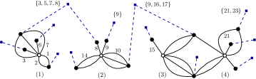
$\rightarrow$      

Figure 5: Left: an element of $\mathcal{P}(\gamma_{\lambda},\tau)$ for $\lambda=\{7,7,6,7\}$ and $\tau$ defining a planar bipartite map $(\gamma_{\lambda},\tau)$. The blue vertices represent the blocks of $\pi^{\prime}$. Right: the corresponding tree in $\mathcal{T}(\gamma_{\lambda},\tau)$.

From trees to partitions. Consider $(T,\{\mathcal{L}_{i}\}_{1\leq i\leq p},\mathcal{L}^{\mathsf{L}})$ as above, and define

$$\pi^{\prime}=\bigl{\{}\cup_{i\in I}\mathcal{L}_{i}(I)\ \mid\ I\in\mathcal{I}_{i}^{\prime}(T)\bigr{\}}\cup\left(\cup_{1=i}^{k}\mathcal{L}^{\mathsf{L}}(i)\right),$$ (3.31)

that is, to each black vertex $I\in\mathcal{I}(T)$ we associate a block of $\pi^{\prime}$: if $\lvert I\rvert>1$ then the corresponding block of $\pi^{\prime}$ is the union of the blocks of $\Pi(\tau)$ attributed to the edges incident to that black vertex $I$. As for the black leaves, this is done in a non-distinguishable manner: all the blocks of $\Pi(\tau)$ associated to black leaves are also blocks of $\pi^{\prime}$. From the “bijectivity” of the block attributions:

$$\Pi(\tau)=\bigl{\{}\mathcal{L}_{i}(I)\ \mid\ I\in\mathcal{I}^{\prime}(T),i\in I\bigr{\}}\cup\left(\cup_{1=i}^{k}\mathcal{L}^{\mathsf{L}}(i)\right),$$ (3.32)

and $\pi^{\prime}\geq\Pi(\tau)$. If $i\in I\cap I^{\prime}$, where $I,I^{\prime}\in\mathcal{I}^{\prime}(T)$ then $G_{i}$ has elements both in $\cup_{i\in I}\mathcal{L}_{i}(I)$ and $\cup_{i\in I^{\prime}}\mathcal{L}_{i}(I)$, and obvious modifications for black leaves, so the fact that $T$ is connected translates as $\pi^{\prime}\vee(\Pi(\sigma\vee\Pi(\tau)))=1_{n}$.

The fact that $\#(\pi)-\#(\tau)-\#(\pi^{\prime})+\#(\Pi(\tau)\vee\Pi(\sigma))=0$ follows from (3.24), noticing that $\#(\tau)=\sum_{I\in\mathcal{I}(T)}\lvert I\rvert$ and $\#(\pi^{\prime})=\sum_{i}(\lvert\mathcal{I}^{\prime}(T)\rvert+\mathrm{deg}_{T}^{\mathsf{L}}(i))$.

From partitions to trees. Starting from $\pi^{\prime}\in\mathcal{P}(\sigma,\tau)$, we first define $T$ through $\mathcal{I}(T)$. To each block of $\pi^{\prime}$, we associate

$$I_{B}=\{i\in\{1,\ldots,k\}\,\mid\,B\cap G_{i}\neq\emptyset\},$$ (3.33)

and define $\mathcal{I}(T)=\{I_{B}\,\mid\,B\in\pi^{\prime}\}$. We verify that it defines an element of $\mathcal{T}(\sigma,\tau)$. It is seen to be connected because $\pi^{\prime}\vee(\Pi(\sigma\vee\Pi(\tau)))=1_{n}$ and noticing that :

$$i\in I_{B}\cap I_{B^{\prime}}\ \Leftrightarrow\ \exists\,a,b\in G_{i},\ a\in B,b\in B^{\prime}.$$

If $L[\pi^{\prime},\Pi(\sigma)\vee\Pi(\tau);\Pi(\tau)]=0$, a block of $\pi^{\prime}$ and a block $G_{i}$ of $\Pi(\sigma)\vee\Pi(\tau)$ may intersect only if their intersection is precisely a block of $\Pi(\tau)$:

$$\mathrm{If}\,L[\pi^{\prime},\Pi(\sigma)\vee\Pi(\tau);\Pi(\tau)]=0,\ \forall B\in\pi^{\prime},\,[B\cap G_{i}\neq\emptyset\ \Rightarrow\ \exists V\in\Pi(\tau),B\cap G_{i}=V].$$ (3.34)

From this we see that $\mathrm{deg}_{T}(i)=\lvert\{B\in\pi^{\prime}\,\mid\,B\cap G_{i}\neq\emptyset\}\rvert$ is in fact the number of blocks of $\Pi(\tau)$ in $G_{i}$, that is, $\#(\tau_{i})$. It also implies that $\lvert I_{B}\rvert=\#(\tau_{\lvert_{B}})$, and $\sum_{I\in\mathcal{I}(T)}\lvert I\rvert=\#(\tau)$. so that the condition $L[\pi^{\prime},\Pi(\sigma)\vee\Pi(\tau);\Pi(\tau)]=0$ translates to (3.24).

It remains to define the block attributions $\mathcal{L}_{i}$ and $\mathcal{L}^{\mathsf{L}}$:

• $\mathcal{L}_{i}:I_{B}\textrm{ s.t. }\lvert I_{B}\rvert>1\rightarrow B\cap G_{i},\ \forall i\in\{1,\ldots,k\},$ (which, has we have seen, corresponds to a unique block of $\Pi(\tau_{i})$),

• $\mathcal{L}^{\mathsf{L}}:i\rightarrow\{V\in\pi^{\prime}\cap\Pi(\tau),\,V\in G_{i}\}$.

One must verify that the attributions thus defined are “bijective”: let $V\in\Pi(\tau_{i})$. Since $\pi^{\prime}\geq\Pi(\tau_{i})$, $\exists!B\in\pi^{\prime},\,V\subset B\cap G_{i}$, so from (3.34), $V=B\cap G_{i}$. We distinguish two cases: if $\lvert I_{B}\rvert>1$, from the definition we indeed have $V=\mathcal{L}_{i}(I_{B})$. Otherwise $\lvert I_{B}\rvert=1$, so $B$ has empty intersections with all others $G_{j},j\neq i$, so that $B\cap G_{i}=B$. Since $V=B\cap G_{i}$, $V=B$, so that $V\in\pi^{\prime}$. Since $V\in\Pi(\tau)$ and $V\subset G_{i}$, $V\in\mathcal{L}^{\mathsf{L}}(i)$.

Having established this bijection, we may reformulate (3.1) as follows for $\vec{b}=(b,\ldots,b)$, $\sigma=\gamma_{\lambda},\lambda\vdash n$ and $\pi=1_{n}$:

$$\varphi_{p}(b^{\lambda_{1}},\ldots,b^{\lambda_{p}})=\sum_{\begin{subarray}{c}{\tau\in S_{n},}\\[0.90417pt] {g(\gamma_{\lambda},\tau^{-1})=0}\end{subarray}}\sum_{T\in\mathcal{T}(\gamma_{\lambda},\tau)}\sum_{\begin{subarray}{c}{\{\mathcal{L}_{i}\}_{1\leq i\leq p},\ \mathcal{L}^{\mathsf{L}}}\\ {\textrm{bij. attributions}}\end{subarray}}\prod_{I\in\mathcal{I}^{\prime}(T)}\kappa_{\{\lvert\mathcal{L}_{i}(I)\rvert\}_{i\in I}}[b]\prod_{i=1}^{k}\prod_{V\in\mathcal{L}^{\mathsf{L}}(i)}\kappa_{\lvert V\rvert}[b],$$ (3.35)

where $k=\#(\Pi(\gamma_{\lambda})\vee\Pi(\tau))$. We group the terms in the sum by the partition $\tilde{\pi}:=\Pi(\gamma_{\lambda})\vee\Pi(\tau)$:

$$\varphi_{p}(b^{\lambda_{1}},\ldots,b^{\lambda_{p}})=\sum_{k=1}^{p}\sum_{\begin{subarray}{c}{\tilde{\pi}\geq\Pi(\gamma_{\lambda}),}\\[0.60275pt] {\#(\tilde{\pi})=k}\end{subarray}}\sum_{\begin{subarray}{c}{\tau\in S_{n},}\\[0.60275pt] {g(\gamma_{\lambda},\tau^{-1})=0}\\[0.90417pt] {\Pi(\gamma_{\lambda})\vee\Pi(\tau)=\tilde{\pi}}\end{subarray}}\sum_{\begin{subarray}{c}{T\in\mathcal{T}_{k}}\\ {\mathrm{deg}_{T}(i)=\#(\tau_{i})}\end{subarray}}\sum_{\begin{subarray}{c}{\{\mathcal{L}_{i}\}_{i},\ \mathcal{L}^{\mathsf{L}}}\\ {\textrm{bij. att.}}\end{subarray}}$$

$$\hskip 199.16928pt\times\prod_{I\in\mathcal{I}^{\prime}(T)}\kappa_{\{\lvert\mathcal{L}_{i}(I)\rvert\}_{i\in I}}[b]\prod_{i=1}^{k}\prod_{V\in\mathcal{L}^{\mathsf{L}}(i)}\kappa_{\lvert V\rvert}[b],$$

where we label the blocks of $\tilde{\pi}$ by the minimum as $G_{1},\ldots,G_{k}$, and $\tau_{i}=\tau_{\lvert_{G_{i}}}$. We can now exchange the sums over $T$ and $\tau$:

$$\varphi_{p}(b^{\lambda_{1}},\ldots,b^{\lambda_{p}})=\sum_{k=1}^{p}\sum_{\begin{subarray}{c}{\tilde{\pi}\geq\Pi(\gamma_{\lambda}),}\\[0.60275pt] {\#(\tilde{\pi})=k}\end{subarray}}\sum_{T\in\mathcal{T}_{k}}\sum_{\begin{subarray}{c}{\tau\in S_{n},}\\[0.60275pt] {g(\gamma_{\lambda},\tau^{-1})=0}\\[0.90417pt] {\Pi(\gamma_{\lambda})\vee\Pi(\tau)=\tilde{\pi}}\\[0.90417pt] {\#(\tau_{i})=\mathrm{deg}_{T}(i)}\end{subarray}}\sum_{\begin{subarray}{c}{\{\mathcal{L}_{i}\}_{i},\,\mathcal{L}^{\mathsf{L}}}\\ {\textrm{bij. att.}}\end{subarray}}\ \prod_{I\in\mathcal{I}^{\prime}(T)}\kappa_{\{\lvert\mathcal{L}_{i}(I)\rvert\}_{i\in I}}[b]\prod_{i=1}^{k}\prod_{V\in\mathcal{L}^{\mathsf{L}}(i)}\kappa_{\lvert V\rvert}[b],$$ (3.36)

and then group the terms by the cardinals of the $\mathcal{L}_{i}(I)$ for $I,i$, and of the blocks of $\mathcal{L}^{\mathsf{L}}(i)$, in order to factorize the product of cumulants:

$$\varphi_{p}(b^{\lambda_{1}},\ldots,b^{\lambda_{p}})=\sum_{k=1}^{p}\sum_{\begin{subarray}{c}{\tilde{\pi}\geq\Pi(\gamma_{\lambda}),}\\[0.60275pt] {\#(\tilde{\pi})=k}\end{subarray}}\sum_{T\in\mathcal{T}_{k}}\sum_{i=1}^{k}\sum_{\begin{subarray}{c}{\{j_{i}^{I}\geq 1\}_{I\in\mathcal{I}^{\prime}_{i}(T)}}\\ {k_{1}^{(i)},\ldots,k_{\lvert G_{i}\rvert}^{(i)}\geq 0,\ \ \sum_{a}k_{a}^{(i)}=\mathrm{deg}_{T}^{\mathsf{L}}(i)}\\ {\sum_{I\in\mathcal{I}_{i}(T)}j_{i}^{I}+\sum_{a=1}^{\lvert G_{i}\rvert}ak_{a}^{(i)}={\lvert G_{i}\rvert}}\end{subarray}}$$

$$\hskip 85.35826pt\times\prod_{I\in\mathcal{I}^{\prime}(T)}\kappa_{\{j_{i}^{I}\}_{i\in I}}[b]\prod_{i=1}^{k}\prod_{a=1}^{\lvert G_{i}\rvert}\kappa_{a}[b]^{k_{a}^{(i)}}\sum_{\begin{subarray}{c}{\tau\in S_{n},}\\[0.60275pt] {g(\gamma_{\lambda},\tau^{-1})=0}\\[0.90417pt] {\Pi(\gamma_{\lambda})\vee\Pi(\tau)=\tilde{\pi}}\\[1.20552pt] {\Lambda(\tau_{i})=\Lambda_{\{k_{a}^{(i)}+q_{a}^{(i)}\}_{a}}}\end{subarray}}\sum_{\begin{subarray}{c}{\{\mathcal{L}_{i}\}_{i},\ \mathcal{L}^{\mathsf{L}}}\\ {\textrm{bij. att.}}\\ {\forall i\in\mathcal{I}_{i}^{\prime}(T),\,\lvert\mathcal{L}_{i}(I)\rvert=j_{i}^{I}}\\ {\forall i,\,\mathcal{L}^{\mathsf{L}}(i)\textrm{ has }k_{a}^{(i)}\textrm{ elts. of size }a}\end{subarray}}1,$$

where we recall that $\mathrm{deg}_{T}^{\mathsf{L}}(i)$ is the number of black leaves incident to the white vertex $i$, and $q_{a}^{(i)}$ is the number of $j_{i}^{I}$ equal to $a$ when $I$ spans $\mathcal{I}_{i}^{\prime}(T)$. The number of attributions is found to be:

$$\sum_{\begin{subarray}{c}{\{\mathcal{L}_{i}\}_{i},\ \mathcal{L}^{\mathsf{L}}}\\ {\textrm{bij. att.}}\\ {\forall i\in\mathcal{I}_{i}^{\prime}(T),\,\lvert\mathcal{L}_{i}(I)\rvert=j_{i}^{I}}\\ {\forall i,\,\mathcal{L}^{\mathsf{L}}(i)\textrm{ has }k_{a}^{(i)}\textrm{ elts. of size }a}\end{subarray}}1\ =\ \prod_{i=1}^{k}\prod_{a=1}^{\lvert G_{i}\rvert}\binom{k_{a}^{(i)}+q_{a}^{(i)}}{k_{a}^{(i)}}q_{a}^{(i)}!\,.$$ (3.37)

Indeed, the blocks of $\Pi(\tau_{i})$ are fixed and we know from the condition on $\Lambda(\tau_{i})$ that for each $a$, there are $k_{a}^{(i)}+q_{a}^{(i)}$ edges incident to the white vertex $i$ that are attributed a block of $\Pi(\tau_{i})$ of size $a$. We have to count all possible ways to attribute for every $a,$ $k_{a}^{i}$ of them to the set of black leaves (without providing the information on which black leaf as they can’t be distinguished), and among the $q_{a}{(i)}$ remaining ones, to decide to which non-leaf black vertex they are assigned to (the edges incident to black leaf vertices are distinguishable). There are $q_{a}{(i)}!$ ways to do so, thus the result above. This quantity factorizes as it is independent from $\tau$, and it remains to see that denoting by $\gamma^{i}_{\lambda}=(\gamma_{\lambda}){\lvert_{{}_{G_{i}}}}$:

$$\sum_{\begin{subarray}{c}{\tau\in S_{n},}\\[0.60275pt] {g(\gamma_{\lambda},\tau^{-1})=0}\\[0.90417pt] {\Pi(\gamma_{\lambda})\vee\Pi(\tau)=\tilde{\pi}}\\[1.20552pt] {\forall i,\,\Lambda(\tau_{i})=\Lambda_{\{k_{a}^{(i)}+q_{a}^{(i)}\}_{a}}}\end{subarray}}1\ =\ \prod_{i=1}^{k}\sum_{\begin{subarray}{c}{\tau_{i}\in S_{n},}\\[0.60275pt] {g(\gamma^{i}_{\lambda},\tau_{i}^{-1})=0}\\[0.90417pt] {\Pi(\gamma^{i}_{\lambda})\vee\Pi(\tau_{i})=1_{\lvert G_{i}\rvert}}\\[1.20552pt] {\Lambda(\tau_{i})=\Lambda_{\{k_{a}^{(i)}+q_{a}^{(i)}\}_{a}}}\end{subarray}}1\ =\ \prod_{i=1}^{k}\mathcal{M}\left(\lambda_{\lvert_{i}};\Lambda_{\{k_{a}^{(i)}+q_{a}^{(i)}\}_{a}}\right),$$ (3.38)

where we recall that $\lambda_{\lvert_{i}}=\Lambda\bigl{(}(\gamma_{\lambda}){\lvert_{{}_{G_{i}}}}\bigr{)}$. The theorem follows by replacing the sum over trees $T\in\mathcal{T}_{k}$ by a sum over trees $T^{\prime}\in\mathcal{G}_{k}$ (with no black leaves) and a sum over $l_{i}\geq 0$, where $\mathrm{deg}_{T}^{\mathsf{L}}(i)=l_{i}$, and $\mathcal{I}^{\prime}(T)=\mathcal{I}(T^{\prime})$. ∎

As an example, for $p=2$ there are two trees in $\mathcal{G}_{2}$ and the formula in the theorem reads:

$$\varphi_{2}(b^{\lambda_{1}},b^{\lambda_{2}})=\sum_{\begin{subarray}{c}{\{k_{i}\geq 0\}_{1\leq i\leq n}}\\[0.60275pt] {\sum_{i=1}^{n}ik_{i}=n}\end{subarray}}\prod_{i=1}^{n}\kappa_{i}[b]^{k_{i}}\mathcal{M}\Bigl{(}{\{\lambda_{1},\lambda_{2}\}};\Lambda_{\{k_{a}^{(i)}\}_{a}}\Bigr{)}$$

$$+\sum_{\begin{subarray}{c}{j_{1},j_{2}\geq 1}\end{subarray}}\kappa_{\{j_{1},j_{2}\}}[b]\prod_{i=1}^{2}\Biggl{(}\sum_{\begin{subarray}{c}{k_{1}^{(i)},\ldots,k_{\lambda_{i}}^{(i)}\geq 0}\\ {\sum_{a=1}^{\lambda_{i}}ak_{a}^{(i)}=\lambda_{i}-j_{i}}\end{subarray}}\frac{(k_{j_{i}}^{(i)}+1)!}{k_{j_{i}}^{(i)}!}\prod_{a=1}^{\lambda_{i}}\kappa_{a}[b]^{k_{a}^{(i)}}\frac{\lambda_{i}!}{(\lambda_{i}-\sum_{a}k_{a}^{(i)})!\prod_{a\neq j}k_{a}!(k_{j_{i}}+1)!}\Biggr{)},$$

where $\sigma_{i}=\sigma_{\lvert_{G_{i}}}$, and we have used the fact that (see e.g.[22])

$$\mathcal{M}\bigl{(}n;\Lambda_{\{k_{a}\}_{a}}\bigr{)}=\frac{n!}{(n+1-\sum_{a}k_{a})!\prod_{a}k_{a}^{(i)}!}.$$ (3.39)

This simplifies to

$$\varphi_{2}(b^{\lambda_{1}},b^{\lambda_{2}})=\sum_{\begin{subarray}{c}{\{k_{i}\geq 0\}_{1\leq i\leq n}}\\[0.60275pt] {\sum_{i=1}^{n}ik_{i}=n}\end{subarray}}\prod_{i=1}^{n}\kappa_{i}[b]^{k_{i}}\mathcal{M}\Bigl{(}{\{\lambda_{1},\lambda_{2}\}};\Lambda_{\{k_{a}^{(i)}\}_{a}}\Bigr{)}$$

$$\hskip 85.35826pt+\sum_{\begin{subarray}{c}{j_{1},j_{2}\geq 1}\end{subarray}}\kappa_{\{j_{1},j_{2}\}}[b]\prod_{i=1}^{2}\Biggl{(}\sum_{\begin{subarray}{c}{k_{1}^{(i)},\ldots,k_{\lambda_{i}}^{(i)}\geq 0}\\ {\sum_{a=1}^{\lambda_{i}}ak_{a}^{(i)}=\lambda_{i}-j_{i}}\end{subarray}}\prod_{a=1}^{\lambda_{i}}\kappa_{a}[b]^{k_{a}^{(i)}}\frac{\lambda_{i}!}{(\lambda_{i}-\sum_{a}k_{a}^{(i)})!\prod_{a}k_{a}!}\Biggr{)}.$$

The bijection between partitions satisfying a forest-condition $L=0$ and labeled bipartite trees in the proof of Thm. 3.5 will be used in several occasions in Sec. 4, and may take simpler forms, depending on the cases and choices of variables in the sums. Let us formalize it in a simpler form. For $\pi\in\mathcal{P}(n)$, we let $\mathcal{G}_{\pi}$ be the set of bipartite trees with white vertices labeled by the blocks of $\pi$ (to avoid labeling these blocks). The black vertices - given by the set $\mathcal{I}(T)$ - are now sets of strictly more than one blocks of $\pi$. We consider some series of numbers $c(\{i_{j}\})_{1\leq j\leq q}$ for $q\geq 1$ and all $i_{j}\geq 1$.

Corollary 3.6.

Consider $\bar{\pi},\tilde{\pi}\in\mathcal{P}(n)$ satisfying $\tilde{\pi}\geq\bar{\pi}$ and let $k=\#(\tilde{\pi}\vee\bar{\pi})$. The following identity holds:

$$\sum_{\begin{subarray}{c}{\pi^{\prime\prime}\geq\bar{\pi}}\\ {\tilde{\pi}\vee\pi^{\prime\prime}=1_{n}}\\[0.90417pt] {L[\pi^{\prime\prime},\,\tilde{\pi}\,;\,\bar{\pi}]=0}\end{subarray}}\prod_{G\in\pi^{\prime\prime}}c(\{\lvert B\rvert\}_{B\in\bar{\pi}})=\sum_{T\in\mathcal{G}_{k}}\sum_{G\in\tilde{\pi}\vee\bar{\pi}}\sum_{\begin{subarray}{c}{\{B_{G}^{I}\}_{I\in\mathcal{I}_{G}(T)}}\\[0.60275pt] {\mathrm{s.t.}\,B_{G}^{I}\in\bar{\pi}_{\lvert_{G}}}\\[0.90417pt] {\mathrm{2-by-2\ different}}\end{subarray}}\prod_{I\in\mathcal{I}(T)}\ c({\{\lvert B_{G}^{I}\rvert\}_{G\in I}})\prod_{G\in\tilde{\pi}\vee\bar{\pi}}\prod_{\begin{subarray}{c}{B\in\bar{\pi}}\\ {B\notin\{B_{G}^{I}\}_{I\in\mathcal{I}_{G}}}\end{subarray}}c(\lvert B\rvert).$$

In particular, we may apply this to reformulate (3.3), which we recall to be:

$$\Gamma[\nu,1_{n},\tilde{\pi}]=\sum_{\begin{subarray}{c}{\pi^{\prime\prime}\geq\Pi(\nu)}\\ {\tilde{\pi}\vee\pi^{\prime\prime}=1_{n}}\\[0.90417pt] {L[\pi^{\prime\prime},\,\tilde{\pi}\,;\,\Pi(\nu)]=0}\end{subarray}}\ \prod_{G\in\pi^{\prime\prime}}\gamma(\nu_{|_{G}})\;.$$ (3.40)

This can thus be expressed as:

$$\Gamma[\nu,1_{n},\tilde{\pi}]=\sum_{T\in\mathcal{G}_{k}}\sum_{G\in\tilde{\pi}\vee\Pi(\nu)}\sum_{\begin{subarray}{c}{\{B_{G}^{I}\}_{I\in\mathcal{I}_{G}(T)}}\\[0.60275pt] {\mathrm{s.t.}\,B_{G}^{I}\in\Pi(\nu_{\lvert_{G}})}\\[0.90417pt] {\mathrm{2-by-2\ different}}\end{subarray}}\prod_{I\in\mathcal{I}(T)}\ \gamma({\{\lvert B_{G}^{I}\rvert\}_{G\in I}})\prod_{\begin{subarray}{c}{B\in\Pi(\nu)}\\ {B\notin\{B_{G}^{I}\}_{I\in\mathcal{I}_{G}}}\end{subarray}}C_{\lvert B\rvert-1},$$

where $C_{k}=\binom{2k}{k}/(k+1)$ is the $k$th Catalan number, and $\gamma$ are rescaled monotone Hurwitz numbers:

$$\gamma(\{q_{G}\}_{G\in I})=(-1)^{\lvert I\rvert+1}\frac{(2\sum_{G\in I}q_{G}+\lvert I\rvert-3)!}{(2\sum_{G\in I}q_{G})!}\prod_{G\in I}\frac{(2q_{G})!}{q_{G}!(q_{G}-1)!},$$

where $\lvert I\rvert$ is the valency of the black vertex $I$.

4 Functional relations

4.1 Functional relations for factorized permutations

Instead of pursuing with (3.5), where the number of planar bipartite maps with prescribed vertex valencies $\mathcal{M}$ causes difficulties, we rather follow the strategy of [9], providing a second tree reformulation from factorized permutations.

Recall that a function $f:\pi\geq\sigma\rightarrow f(\pi,\sigma)$ is said to be multiplicative if $f(\pi,\sigma)=\prod_{G\in\pi}f(1_{{\lvert G\rvert}},\sigma_{\mid{{}_{\lvert G\rvert}}})$, and $f(1_{n},\sigma)$ depends only on $\Lambda(\sigma)$. Also recall that

$$L[\pi^{\prime},\Pi(\sigma)\vee\Pi(\tau);\Pi(\tau)]=\#(\pi)-\#(\tau)-\#(\pi^{\prime})+\#(\Pi(\tau)\vee\Pi(\sigma)).$$

If $\lambda\vdash n$, $\gamma_{\lambda}=\gamma_{\lambda_{1},\ldots,\lambda_{p}}\in S_{n}$ is given in (2.1), where $p=\#(\lambda)$, and we denote by

$$\mathrm{NC}(\lambda_{1})\times\cdots\times\mathrm{NC}(\lambda_{p})=\Bigl{\{}\tau\in S_{n}\,\mid\,\Pi(\tau)\leq\Pi(\gamma_{\lambda}),\,\textrm{and for }1\leq i\leq p,\ g\bigl{(}\tau_{i},\gamma_{i}^{-1}\bigr{)}=0\Bigr{\}},$$ (4.1)

where $\tau_{i}$ and $\gamma_{i}$ are the restrictions of $\tau$ and $\gamma$ to $\{\sum_{j<i}\lambda_{j}+1,\ldots,\sum_{j<i}\lambda_{j}+\lambda_{i}\}$ (which is the $i$th block of $\Pi(\gamma_{\lambda})$ when labeled by the minimum). We also use the notation $\tau=\tau_{1}\times\ldots\times\tau_{p}$, $\tau_{i}\in\mathrm{NC}(\lambda_{i})$. The following is a generalization at arbitrary order of Prop. 6.2 in [9].

Theorem 4.1.

Let $g:\pi\geq\sigma\rightarrow g(\pi,\sigma)$ be a multiplicative function and $p\geq 1$, and consider the generating function

$$H_{p}(X_{1},\ldots,X_{p})=\delta_{p,1}+\sum_{k_{1},\ldots,k_{p}\geq 1}\tilde{\alpha}_{k_{1},\ldots,k_{p}}X_{1}^{k_{1}}\cdots X_{p}^{k_{p}},\qquad\ \ \tilde{\alpha}_{k_{1},\ldots,k_{p}}=g(1_{k_{1}+\cdots+k_{p}},\gamma_{k_{1},\ldots,k_{p}}).$$

Introduce the following numbers: for $p\geq 1$ and $\lambda_{1},\ldots,\lambda_{p}\geq 1$,

$$\beta_{\lambda_{1},\ldots,\lambda_{p}}=\sum_{\begin{subarray}{c}{\tau\in\mathrm{NC}(\lambda_{1})\times\cdots\times\mathrm{NC}(\lambda_{p})}\end{subarray}}\hskip 5.69046pt\sum_{\begin{subarray}{c}{\pi^{\prime}\geq\Pi(\tau)}\\[0.90417pt] {\pi^{\prime}\vee\Pi(\gamma_{\lambda})=1_{n}}\\[0.90417pt] {L[\pi^{\prime},\,\Pi(\gamma_{\lambda})\vee\Pi(\tau)\,;\,\Pi(\tau)]=0}\end{subarray}}g(\pi^{\prime},\tau),$$ (4.2)

and the corresponding generating function:

$$B_{p}(X_{1},\ldots,X_{p})=\delta_{p,1}+\sum_{\lambda_{1},\ldots,\lambda_{p}\geq 1}\beta_{\lambda_{1},\ldots,\lambda_{p}}X_{1}^{\lambda_{1}}\cdots X_{p}^{\lambda_{p}}.$$

Then we have the following functional relations:

$$B_{p}(X_{1},\ldots,X_{p})=\sum_{T\in\mathcal{G}_{p}}\biggl{(}\prod_{i=1}^{p}X_{i}^{\mathrm{d}_{T}(i)-1}\frac{\mathrm{d}^{\mathrm{d}_{T}(i)-1}}{\mathrm{d}X_{i}^{\mathrm{d}_{T}(i)-1}}\biggr{)}\Biggl{\{}\prod_{i=1}^{p}{\frac{\mathrm{d}Y_{i}}{\mathrm{d}X_{i}}}\prod_{I\in\mathcal{I}(T)}\ \frac{H_{\lvert I\rvert}\bigl{(}Y_{I}\bigr{)}}{\prod_{i\in I}B_{1}(X_{i})}\Biggr{\}},$$ (4.3)

where $\mathrm{d}_{T}(i)=\mathrm{deg}_{T}(i)$, $Y_{I}=\{Y_{i}\}_{i\in I}$, and $Y_{i}=X_{i}B_{1}(X_{i})$.

At the level of the coefficients, these relations are equivalent to

$$\beta_{\lambda_{1},\ldots,\lambda_{p}}=\sum_{T\in\mathcal{G}_{p}}\Biggl{(}\sum_{i=1}^{p}\sum_{l_{i}\geq 0}\sum_{\begin{subarray}{c}{\{j_{i}^{I}\geq 1\}_{I\in\mathcal{I}_{i}(T)}}\\ {k_{1}^{(i)},\ldots,k_{\lambda_{i}}^{(i)}\geq 0,\ \ \sum_{a}k_{a}^{(i)}=l_{i}}\\ {\sum_{I\in\mathcal{I}_{i}(T)}j_{i}^{I}+\sum_{a=1}^{\lambda_{i}}ak_{a}^{(i)}={\lambda_{i}}}\end{subarray}}\Biggr{)}\Biggl{(}\prod_{I\in\mathcal{I}(T)}\ \tilde{\alpha}_{\{j_{i}^{I}\}_{i\in I}}\Biggr{)}$$

$$\hskip 213.39566pt\times\left(\prod_{i=1}^{n}\frac{\lambda_{i}!}{(\lambda_{i}+1-l_{i}-\mathrm{deg}_{T}(i))!}\prod_{a=1}^{\lambda_{i}}\frac{1}{k_{a}^{(i)}!}\ \tilde{\alpha}_{a}^{k_{a}^{(i)}}\right).$$

Proof.

We can adapt the proof of Th. 3.5. The difference lies in the fact that here, $\Pi(\tau)\vee\Pi(\gamma_{\lambda})=\Pi(\gamma_{\lambda})$, so that the bijection reduces to trees in $\mathcal{T}_{p}$ with one white vertex per block of $\Pi(\gamma_{\lambda})$. Using in addition the formula (3.39):

$$\beta_{\lambda_{1},\ldots,\lambda_{p}}=\sum_{T\in\mathcal{G}_{p}}\Biggl{(}\sum_{i=1}^{p}\sum_{l_{i}\geq 0}\sum_{\begin{subarray}{c}{\{j_{i}^{I}\geq 1\}_{I\in\mathcal{I}_{i}(T)}}\\ {k_{1}^{(i)},\ldots,k_{\lambda_{i}}^{(i)}\geq 0,\ \ \sum_{a}k_{a}^{(i)}=l_{i}}\\ {\sum_{I\in\mathcal{I}_{i}(T)}j_{i}^{I}+\sum_{a=1}^{\lambda_{i}}ak_{a}^{(i)}={\lambda_{i}}}\end{subarray}}\Biggr{)}\Biggl{(}\prod_{I\in\mathcal{I}(T)}\ \tilde{\alpha}_{\{j_{i}^{I}\}_{i\in I}}\Biggr{)}$$

$$\hskip 85.35826pt\times\left(\prod_{i=1}^{n}\frac{\lambda_{i}!}{(\lambda_{i}+1-\sum_{a}k_{a}^{(i)}+q_{a}^{(i)})\prod_{a}(k_{a}^{(i)}+q_{a}^{(i)})!}\prod_{a=1}^{\lambda_{i}}\frac{\bigl{(}k_{a}^{(i)}+q_{a}^{(i)}\bigr{)}!}{k_{a}^{(i)}!}\,\tilde{\alpha}_{a}^{k_{a}^{(i)}}\right),$$

where $q_{a}^{(i)}$ is the number of integers in the set $\{j_{i}^{I}\}_{I\in\mathcal{I}_{i}(T)}$ that are equal to $a$. In particular, $\sum_{a}q_{a}^{(i)}=\mathrm{deg}_{T}(i)$. The derivation of the functional formulas is unchanged from Sec. 2.6.4. There are only two minor points to be justified. The first one is that nothing changes with the sums starting at $l_{i}\geq 0$ instead of $l_{i}\geq 1$. One verifies that the equation (2.55) is still valid for $l\geq 0$ (and it no longer matters whether $\lambda>j$). The second point to be justified is that we can indeed use Lagrange inversion as in (2.56), which is true because the relation (4.2) is $\beta_{n}=\sum_{\tau\in\mathrm{NC}(n)}g(\Pi(\tau),\tau)$, meaning (see the main theorem in [22]) that $H_{1}(XB_{1}(X))=B_{1}(X)$. ∎

4.2 Factorization

Let us recall here the relations of Thm. 3.1 for $\vec{b}=(b,\ldots,b)$, $\sigma=\gamma_{\lambda},\lambda\vdash n$ and $\pi=1_{n}$:

$$\varphi_{p}(b^{\lambda_{1}},\ldots,b^{\lambda_{p}})=\sum_{\begin{subarray}{c}{\tau\in S_{n},}\\[0.90417pt] {g(\gamma_{\lambda},\tau^{-1})=0}\end{subarray}}\hskip 5.69046pt\sum_{\begin{subarray}{c}{\pi^{\prime}\geq\Pi(\tau)}\\[0.90417pt] {\pi^{\prime}\vee\Pi(\gamma_{\lambda})=1_{n}}\\[0.90417pt] {L[\pi^{\prime},\,\Pi(\gamma_{\lambda})\vee\Pi(\tau)\,;\,\Pi(\tau)]=0}\end{subarray}}\kappa(\pi^{\prime},\tau)[b].$$ (4.4)

Considering $f:\pi\geq\sigma\rightarrow g(\pi,\sigma)$ a multiplicative function and $p\geq 1$, and some numbers defined for $p\geq 1$ and $\lambda_{1},\ldots,\lambda_{p}\geq 1$ by (see the left of Fig. 5):

$$\beta_{\lambda_{1},\ldots,\lambda_{p}}=\sum_{\begin{subarray}{c}{\tau\in S_{n},}\\[0.90417pt] {g(\gamma_{\lambda},\tau^{-1})=0}\end{subarray}}\hskip 5.69046pt\sum_{\begin{subarray}{c}{\pi^{\prime}\geq\Pi(\tau)}\\[0.90417pt] {\pi^{\prime}\vee\Pi(\gamma_{\lambda})=1_{n}}\\[0.90417pt] {L[\pi^{\prime},\,\Pi(\gamma_{\lambda})\vee\Pi(\tau)\,;\,\Pi(\tau)]=0}\end{subarray}}f(\pi^{\prime},\tau),$$ (4.5)

for instance $\beta_{\lambda_{1},\ldots,\lambda_{p}}:=\varphi_{p}(b^{\lambda_{1}},\ldots,b^{\lambda_{p}})$ and $f(1_{k_{1}+\cdots+k_{p}},\gamma_{k_{1},\ldots,k_{p}}):=\kappa_{k_{1},\ldots,k_{p}}[b]$, we can always opt for a summation over factorized permutations $\mathrm{NC}(\lambda_{1})\times\cdots\times\mathrm{NC}(\lambda_{p})$ by a generalization of the trick of Sec. 6 of [9].

If $\tau=\tau_{1}\times\ldots\times\tau_{p}$, where $\tau_{i}\in\mathrm{NC}(\lambda_{i})$ and $B$ a block of $\pi^{\prime}\geq\Pi(\tau)$, we let as in (3.33):

$$I_{B}=\{i\in\{1,\ldots,p\}\,\mid\,B\cap\Pi(\tau_{i})\neq\emptyset\}.$$ (4.6)

If $I\subset\{1,\ldots,p\}$, we let $\mathcal{P}^{*}(I)$ be the set of partitions of the elements in $I$ that have more than $\lvert I\rvert$ blocks. For $d\geq 1$ and $\tau\in S_{d}$, we let $\mathrm{NS}(\tau)$ be the subset

$$\mathrm{NS}(\tau)\subset\Bigl{\{}\nu\in S_{d}\mid g(\nu,\tau)=0,\Pi(\tau)\vee\Pi(\nu)=1_{d}\Bigr{\}}$$

for which there are no white cut-vertices, which we have called planar non-separable hypermaps (see Sec. 2.4). Note that if $\tau=\eta$ has just one cycle, $\mathrm{NS}(\eta)=\{\eta^{-1}\}$ has just one element.

Theorem 4.2.

The relations (4.5) defining $\beta_{\lambda_{1},\ldots,\lambda_{p}}$ can be expressed equivalently as:

$$\beta_{\lambda_{1},\ldots,\lambda_{p}}=\sum_{\begin{subarray}{c}{\tau=\bigtimes_{i=1}^{p}\tau_{i}}\\[0.90417pt] {\tau_{i}\in\mathrm{NC}(\lambda_{i})}\end{subarray}}\hskip 5.69046pt\sum_{\begin{subarray}{c}{\pi^{\prime}\geq\Pi(\tau)}\\[0.90417pt] {\pi^{\prime}\vee\Pi(\gamma_{\lambda})=1_{n}}\\[0.90417pt] {L[\pi^{\prime},\,\Pi(\gamma_{\lambda})\,;\,\Pi(\tau)]=0}\end{subarray}}g(\pi^{\prime},\tau),$$ (4.7)

where $g(\pi^{\prime},\tau)$ is multiplicative over the blocks of $\pi^{\prime}$, and such that if $B\in\pi^{\prime}$:

$$g(1_{\lvert B\rvert},\tau_{\lvert_{B}})=f\bigl{(}\Pi(\tau_{\lvert_{B}}),\tau_{\lvert_{B}}\bigr{)}+\sum_{\bar{\pi}\in\mathcal{P}^{*}(I_{B})}\bar{g}_{\bar{\pi}}(\tau_{\lvert_{B}}),$$ (4.8)

where for $G\in\bar{\pi}$, we define $\tau_{G}=\bigtimes_{i\in G}\bigl{(}{\tau_{i}}_{\lvert_{B}}\bigr{)}$ (which is also $\tau_{G}={\gamma_{\lambda}}_{\lvert_{G}}$), and:

$$\bar{g}_{\bar{\pi}}(\tau_{\lvert_{B}})=\sum_{\begin{subarray}{c}{\nu=\bigtimes_{G\in\bar{\pi}}\nu_{G}}\\[0.90417pt] {\nu_{G}\in\mathrm{NS}(\tau_{G})}\end{subarray}}\ \sum_{\begin{subarray}{c}{\pi^{\prime\prime}\geq\Pi(\nu)}\\[0.90417pt] {\pi^{\prime\prime}\vee\Pi(\tau_{\lvert_{B}})=1_{\lvert B\rvert}}\\[0.90417pt] {L[\pi^{\prime\prime},\,\Pi(\tau_{\lvert_{B}})\vee\Pi(\nu)\,;\,\Pi(\nu)]=0}\end{subarray}}f(\pi^{\prime\prime},\nu).$$ (4.9)

See the end of the present subsection for the proof. If $\bar{\pi}$ has a single block, this simplifies to:

$$\tilde{f}(\tau_{\lvert_{B}}):=\bar{g}_{1_{\lvert I_{B}\rvert}}(\tau_{\lvert_{B}})=\sum_{\nu\in\mathrm{NS}\left(\tau_{\lvert_{B}}\right)}\ f(\Pi(\nu),\nu).$$ (4.10)

Weight of a vertex as sum over trees.

We now set $f(1_{k_{1}+\cdots+k_{p}},\gamma_{k_{1},\ldots,k_{p}})=\kappa_{k_{1},\ldots,k_{p}}[b]$ and drop the explicit dependency in $[b]$ from now on. Let $\mathcal{G}_{\bar{\pi}}$ be the set of bipartite trees with white (square) vertices labeled by the blocks of $\bar{\pi}$ (to avoid labeling these blocks with integers), so that the non-white vertices of the tree, given by the set $\mathcal{I}(T)$ - now blue squares to avoid confusion - are sets of strictly more than one blocks of $\bar{\pi}$. From (3.36) in the proof of Thm. 3.5 (see also Cor. 3.6), we may rewrite (4.9) as:

$$\bar{g}_{\bar{\pi}}=\sum_{T\in\mathcal{G}_{\bar{\pi}}}\bar{\kappa}_{\bar{\pi},T}$$ (4.11)

where recalling that $\tau_{G}=\bigtimes_{i\in G}\bigl{(}{\tau_{i}}_{\lvert_{B}}\bigr{)}$ (which is also $\tau_{G}={\gamma_{\lambda}}_{\lvert_{G}}$),

$$\bar{\kappa}_{\bar{\pi},T}(\tau_{\lvert_{B}})=\sum_{\begin{subarray}{c}{\nu=\bigtimes_{G\in\bar{\pi}}\nu_{G}}\\[0.90417pt] {\nu_{G}\in\mathrm{NS}(\tau_{G})}\\[0.90417pt] {\#(\nu_{G})\geq\mathrm{deg}_{T}(G)}\end{subarray}}\ \sum_{\begin{subarray}{c}{\{\mathcal{L}_{G}\}_{G}}\\ {\textrm{inj. att.}}\end{subarray}}\ \prod_{K\in\mathcal{I}(T)}\kappa_{\{\lvert\mathcal{L}_{G}(K)\rvert\}_{G\in K}}\ \prod_{G\in\bar{\pi}}\prod_{\begin{subarray}{c}{V\in\Pi(\nu_{G})}\\ {V\notin\mathcal{L}_{G}(\mathcal{I}_{G}(T))}\end{subarray}}\kappa_{\lvert V\rvert},$$ (4.12)

in which $\mathcal{I}(T)=\cup_{G}\mathcal{I}_{G}(T)$, and $\mathcal{I}_{G}(T)$ is the set of blue square vertices of the tree incident to the white square vertex $G$, and for each white square vertex $G\in\bar{\pi}$, $\mathcal{L}_{G}$ is a choice of injective attribution of the edges incident to that vertex to the cycles of $\nu_{G}$:

$$\forall G\in\bar{\pi},\ \mathcal{L}_{G}:\mathcal{I}_{G}(T)\rightarrow\Pi(\nu_{G}),$$

which can also be written as in Cor. 3.6. The sums over $k$ and $\tilde{\pi}$ in (3.36) are no longer needed, as $\tilde{\pi}$ is fixed to $\bar{\pi}=\Pi(\nu)\vee\Pi(\tau)$, and we have chosen to sum over trees in $\mathcal{G}_{p}$ instead of $\mathcal{T}_{p}$, so that the attributions are only injective.

For $T$ the tree with one blue vertex $\lvert\mathcal{I}(T)\rvert=1$, we denote by $\bar{\kappa}_{\bar{\pi}}:=\bar{\kappa}_{\begin{subarray}{c}{\bar{\pi},T},\,\mathrm{s.t.}\,{\lvert\mathcal{I}(T)\rvert=1}\end{subarray}}$. This sum then simplifies to:

$$\bar{\kappa}_{\bar{\pi}}(\tau_{\lvert_{B}})=\sum_{\begin{subarray}{c}{\nu=\bigtimes_{G\in\bar{\pi}}\nu_{G}}\\[0.90417pt] {\nu_{G}\in\mathrm{NS}(\tau_{G})}\end{subarray}}\ \sum_{\begin{subarray}{c}{F=\bigcup_{G\in\bar{\pi}}F_{G}}\\ {F_{G}\in\Pi(\nu_{G})}\end{subarray}}\ \kappa(1_{\lvert F\rvert},\nu_{\lvert_{F}})\prod_{\begin{subarray}{c}{V\in\Pi(\nu)}\\ {V\notin\{F_{G}\}}\end{subarray}}\kappa(1_{\lvert V\rvert},\nu_{\lvert_{V}}).$$ (4.13)

If $\tau_{G}=\eta$ consists of a single cycle, then $\mathrm{NS}(\tau_{G})=\{\eta^{-1}\}$, and the condition $\#(\nu_{G})\geq\mathrm{deg}_{T}(G)$ imposes $\mathrm{deg}_{T}(G)=1$.

To put it in words and pictures, the cost of using factorized permutations $\tau=\tau_{1}\times\ldots\times\tau_{p}$, where $\tau_{i}\in\mathrm{NC}(\lambda_{i})$ (top of Fig. 6) as in (4.7), instead of using generic permutations $\tau$ such that $g(\tau,\gamma_{\lambda}^{-1})=0$, as in (4.5) (left of Fig. 5), is to replace the weight $f\bigl{(}\Pi(\tau_{\lvert_{B}})\bigr{)}$ for the blocks $B\in\pi^{\prime}$ in (4.5) (indicated by the red square vertices in Fig. 6) by a new weight (4.8), which is the sum of the usual weight and a sum of corrections. The corrections for the block $B$ are labeled by $\bar{\pi}\in\mathcal{P}^{\star}(I_{B})$ (thicker edges and colors on the bottom left of Fig. 6) and $T\in\mathcal{G}_{\bar{\pi}}$, where $I_{B}$ is the set of white disc vertices (the cycles of $\gamma_{\lambda}$) involved in this block $B$. The corrections for the partition $\bar{\pi}$ re-create the connections between the white vertices grouped in $\bar{\pi}$, connections that we have removed in factorizing $\tau$. These connections take the form of planar non-separable hypermaps (bottom right of Fig. 6). For a fixed $\bar{\pi}$, the sum over trees (dashed blue edges on the left of Fig. 6) indicates how the higher-order cumulants are arranged. The sum over $\mathcal{L}_{G}$ corresponds to choosing which black vertices of the non-separable hypermaps are grouped in order-$q$ free cumulants (one for each blue vertex with $q$ incident edges). On the bottom right of Fig. 6 for instance, the contribution is

$$\kappa_{2,2,4}[b]\kappa_{2,4}[b]\kappa_{3}[b]\kappa_{2}[b].$$

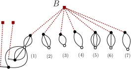
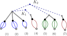
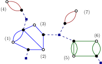
Figure 6: Top: a bipartite map $(\gamma_{\lambda},\tau^{-1})$ with factorized $\tau=\bigtimes_{i=1}^{p}\tau_{i}$, $\tau_{i}\in\mathrm{NC}(\lambda_{i})$ (the black and white vertices and the edges linking them), and tree-like partition $\pi^{\prime}$ with three blocks (the three red vertices). Bottom left: Focusing on the block $B$ of $\pi^{\prime}$, a choice is made of $\bar{\pi}=\{1,2,3\}\{4\}\{5,6\}\{7\}$ (edges in the same blocks carry the same color) and $T$ with two blue vertices $K_{1}=\{1,2,3\}\{4\}$ and $K_{2}=\{1,2,3\}\{5,6\}\{7\}$. Bottom right: choice of a collection of non-separable hypermaps $\{\nu_{G}\}$, one for each block of $\bar{\pi}$, and injective attribution of the edges of $T$ to the cycles of the $\{\nu_{G}\}$. The two cycles which have not been attributed any edge of the tree are attributed a blue leaf. The blue vertices of valency $q$ correspond to order-$q$ free cumulants.

As in Thm. 3.5, we can provide a more detailed expression, useful in Sec. 4.3 for concrete combinatorial computations. Given a planar bipartite map with edges labeled from 1 to $n$ and white vertices labeled with an integer in $G\subset\{1,\ldots,p\}$, we provide a labeling of the black vertices as follows. First consider the white vertex $v_{1}$ with smallest label in $G$, and label from 1 to $\mathrm{deg}(1)$ the black vertices to which $v_{1}$ is connected, according to the smallest label of the edges that connect them. Then go to the white vertex $v_{1}$ with second smallest label in $G$, and label in the same way the black vertices to which $v_{2}$ is connected and that haven’t been labeled yet, and so on, until all the black vertices are labeled.

Letting $I\subset\{1,\ldots,p\}$ and $\mu_{I}=\{\mu_{i}\}_{i\in I}$, $\mu_{i}\geq 1$, as well as $\bar{\pi}\in\mathcal{P}^{\star}(I)$, $G\in\bar{\pi}$ and $\mu_{G}=\{\mu_{i}\}_{i\in G}$, we denote by

$$\mathrm{NS}(\mu_{G}):=\mathrm{NS}(\gamma_{\mu_{G}}).$$

To a bipartite planar map with white vertices given by $\gamma_{\mu_{G}}$ (thus labeled by $G$) and $r$ black vertices given by $\nu_{G}$ (so that $\#(\nu_{G})=r$) and labeled as above, we can therefore associate its adjacency matrix

$$\mathcal{A}(\nu_{G})=\{j_{i,s}\}_{\begin{subarray}{c}{i\in G}\\ {1\leq s\leq r}\end{subarray}},$$

where $j_{i,s}$ is the number of edges connecting the white vertex $i$ and the black vertex $s$. We define the cardinal of the set of planar non-separable hypermaps with fixed permutation $\gamma_{\mu_{G}}$ for the white vertices and fixed adjacency matrix as:

$$\mathcal{N}_{G,r}\left(\{j_{i,s}\}_{\begin{subarray}{c}{i\in G}\\ {1\leq s\leq r}\end{subarray}}\right)=\mathrm{Card}\left\{\nu_{G}\in\mathrm{NS}(\mu_{G}),\,\mu_{G}=\Bigl{(}\sum_{s}j_{i,s}\Bigr{)}_{i\in G},\,\mathcal{A}(\nu_{G})=\{j_{i,s}\}_{i,s}\right\}.$$

With these notations and fixing $T\in\mathcal{G}_{\bar{\pi}}$, we can now follow steps analogous to the proof of Thm. 3.5 (see also Cor. 3.6) and rewrite (4.12) as:

$$\bar{\kappa}_{\bar{\pi},T}(\gamma_{\mu_{I}})=\Biggl{(}\sum_{G\in\bar{\pi}}\sum_{r_{G}\geq\mathrm{deg}_{T}(G)}\ \sum_{\begin{subarray}{c}{\{j_{i,s}\geq 0\}_{\begin{subarray}{c}{i\in G},\,{1\leq s\leq r_{G}}\end{subarray}}}\\[0.60275pt] {\mathrm{s.t.}\sum_{1\leq s\leq r_{G}}j_{i,s}=\mu_{i}}\end{subarray}}\ \sum_{\begin{subarray}{c}{\{\theta({G,K})\}_{K\in\mathcal{I}_{G}(T)}}\\[0.60275pt] {\mathrm{s.t.}\,1\leq\theta({G,K})\leq r_{G}}\\[0.90417pt] {\mathrm{2-by-2\ different}}\end{subarray}}\Biggr{)}$$ (4.14)

$$\hskip 85.35826pt\Biggl{(}\prod_{K\in\mathcal{I}(T)}\kappa_{\left\{j_{G}^{\theta(G,K)}\right\}_{G\in K}}\Biggr{)}\prod_{G\in\bar{\pi}}\Biggl{(}\mathcal{N}_{G,r_{G}}\left(\{j_{i,s}\}_{\begin{subarray}{c}{i\in G}\\ {1\leq s\leq r_{G}}\end{subarray}}\right)\prod_{\begin{subarray}{c}{1\leq s\leq r_{G}}\\ {s\notin\{\theta(G,K)\}_{K\in\mathcal{I}_{G}}}\end{subarray}}\kappa_{j_{G}^{s}}\Biggr{)},$$

where $j_{G}^{s}=\sum_{i\in G}j_{i,s}$. The sum over $\theta(G,K)$ corresponds to the sum over attributions $\mathcal{L}_{G}$. This formula will be useful for looking at concrete examples in Sec. 4.3.

Generating functions.

Having now a sum over factorized $\tau$, we can apply Thm. 4.1. Fixing $I\subset\{1,\ldots,p\}$, we therefore introduce the generating function $H_{\lvert I\rvert}\bigl{(}\{Y_{i}\}_{i\in I}\bigr{)}$ of Thm. 4.1 as

$$H_{\lvert I\rvert}=C_{\lvert I\rvert}+\sum_{\bar{\pi}\in\mathcal{P}^{*}(I)}\bar{H}_{\lvert I\rvert,\bar{\pi}},\qquad\bar{H}_{\lvert I\rvert,\bar{\pi}}=\sum_{T\in\mathcal{G}_{\bar{\pi}}}\bar{C}_{\lvert I\rvert,\bar{\pi},T},$$ (4.15)

where:

$$\bar{C}_{\lvert I\rvert,\bar{\pi},T}\bigl{(}\{Y_{i}\}_{i\in I}\bigr{)}=\sum_{\{\mu_{i}\}_{i\in I}}\ \prod_{i\in I}Y_{i}^{\mu_{i}}\Biggl{[}\sum_{\begin{subarray}{c}{\nu=\bigtimes_{G\in\bar{\pi}}\nu_{G}}\\[0.90417pt] {\nu_{G}\in\mathrm{NS}(\mu_{G})}\\[0.90417pt] {\#(\nu_{G})\geq\mathrm{deg}_{T}(G)}\end{subarray}}\sum_{\begin{subarray}{c}{\{\mathcal{L}_{G}\}_{G}}\\ {\textrm{inj. att.}}\end{subarray}}\ \prod_{K\in\mathcal{I}(T)}\kappa_{\{\lvert\mathcal{L}_{G}(K)\rvert\}_{G\in K}}\ \prod_{G\in\bar{\pi}}\prod_{\begin{subarray}{c}{V\in\Pi(\nu_{G})}\\ {V\notin\mathcal{L}_{G}(\mathcal{I}_{G}(T))}\end{subarray}}\kappa_{\lvert V\rvert}\Biggr{]},$$ (4.16)

In the case where $T$ is the tree with one blue vertex $\lvert\mathcal{I}(T)\rvert=1$, we let: $\bar{C}_{\lvert I\rvert,\bar{\pi}}:=\bar{C}_{\lvert I\rvert,\begin{subarray}{c}{\bar{\pi},T},\,\mathrm{s.t.}\,{\lvert\mathcal{I}(T)\rvert=1}\end{subarray}}$:

$$\bar{C}_{\lvert I\rvert,\bar{\pi}}\bigl{(}\{Y_{i}\}_{i\in I}\bigr{)}=\sum_{\{\mu_{i}\}_{i\in I}}\ \prod_{i\in I}Y_{i}^{\mu_{i}}\ \Biggl{[}\sum_{\bigl{\{}\nu_{G}\in\mathrm{NS}(\mu_{G})\bigr{\}}_{G\in\bar{\pi}}}\ \sum_{\{F_{G}\in\Pi(\nu_{G})\}_{G\in\bar{\pi}}}\kappa_{\{\lvert F_{G}\rvert\}_{G\in\bar{\pi}}}\prod_{\begin{subarray}{c}{V\in\Pi(\bigtimes_{G}\nu_{G})}\\ {V\notin\{F_{G}\}}\end{subarray}}\kappa_{\lvert V\rvert}\Biggr{]},$$ (4.17)

which involves only free cumulants of order $\#(\bar{\pi})$ and one. If $\bar{\pi}$ has a single block, we let $\tilde{C}_{\lvert I\rvert}:=\bar{C}_{\lvert I\rvert,\bar{\pi}}$, which is the generating function for non-separable hypermaps with prescribed vertex valencies, whose hyperedges are weighted by free cumulants $\kappa_{q}$:

$$\tilde{C}_{\lvert I\rvert}\bigl{(}\{Y_{i}\}_{i\in I}\bigr{)}:=\bar{C}_{\lvert I\rvert,\bar{\pi}}\bigl{(}\{Y_{i}\}_{i\in I}\bigr{)}=\sum_{\{\mu_{i}\}_{i\in I}}\ \prod_{i\in I}Y_{i}^{\mu_{i}}\ \Biggl{(}\sum_{\nu\in\mathrm{NS}(\mu_{I})}\ \kappa\bigl{(}\Pi(\nu),\nu\bigr{)}\Biggr{)},$$ (4.18)

where we recall that $\kappa\bigl{(}\Pi(\nu),\nu\bigr{)}=\prod_{G\in\Pi(\nu)}\kappa_{\lvert G\rvert}$.

Proof of the theorem.

We can rewrite (4.8) with a sum over partitions $\pi_{B}\geq\Pi(\tau_{\lvert_{B}})$ instead of $\bar{\pi}\in\mathcal{P}(I_{B}):$

$$g(\pi^{\prime},\tau)=\prod_{B\in\pi^{\prime}}\sum_{\pi_{B}\geq\Pi(\tau_{\lvert_{B}})}\sum_{\begin{subarray}{c}{\nu_{B}=\bigtimes_{G\in\pi_{B}}\nu^{B}_{G}}\\[0.90417pt] {\nu^{B}_{G}\in\mathrm{NS}(\tau_{\lvert_{G}})}\end{subarray}}\ \sum_{\begin{subarray}{c}{\pi^{\prime\prime}_{B}\geq\Pi(\nu_{B})}\\[0.90417pt] {\pi^{\prime\prime}_{B}\vee\Pi(\tau_{\lvert_{B}})=1_{\lvert B\rvert}}\\[0.90417pt] {L[\pi^{\prime\prime}_{B},\,\Pi(\tau_{\lvert_{B}})\vee\Pi(\nu_{B})\,;\,\Pi(\nu_{B})]=0}\end{subarray}}f(\pi^{\prime\prime}_{B},\nu_{B}).$$ (4.19)

For each block $B$, the picture is that of the bottom of Fig. 6: $B$ is a subset of the edges of the bipartite map $(\gamma_{\lambda},\tau^{-1})$, $\pi_{B}$ provides groups of edges of the same color, to each group is associated a non-separable hypermap, and $\pi^{\prime\prime}_{B}$ is a tree -like partition of the black vertices of the non-separable hypermaps (cycles of $\nu_{B}$).

The partitions $\{\pi_{B}\}$ form a partition $\pi$ in $\mathcal{P}(p)$ which satisfies $\Pi(\tau)\leq\pi\leq\pi^{\prime}$. The permutations $\nu_{B}$ also form a permutation $\nu$ in $S_{n}$ which factorizes over the blocks of $\pi$.

$$g(\pi^{\prime},\tau)=\sum_{\begin{subarray}{c}{\pi\in\mathcal{P}(n)}\\ {\pi^{\prime}\geq\pi\geq\Pi(\tau)}\end{subarray}}\ \sum_{\begin{subarray}{c}{\nu=\bigtimes_{G\in\pi}\nu_{G}}\\[0.90417pt] {\nu_{G}\in\mathrm{NS}(\tau_{\lvert_{G}})}\end{subarray}}\ \ \sum_{\begin{subarray}{c}{\pi^{\prime\prime}\in\mathcal{P}(n)}\\ {\pi^{\prime}\geq\pi^{\prime\prime}\geq\Pi(\nu)}\\[0.90417pt] {\forall\,B\in\pi^{\prime},\ \pi^{\prime\prime}_{\lvert_{B}}\vee\Pi(\tau_{\lvert_{B}})=1_{\lvert B\rvert}}\\[0.90417pt] {L[\pi^{\prime\prime},\,\Pi(\tau)\vee\Pi(\nu)\,;\,\Pi(\nu)]=0}\end{subarray}}f(\pi^{\prime\prime},\nu).$$ (4.20)

Note that a consequence of $\nu=\bigtimes_{G\in\pi}\nu_{G}$, $\nu_{G}\in\mathrm{NS}(\tau_{\lvert_{G}})$ is that $\pi=\Pi(\nu)\vee\Pi(\tau)$.

We now want to exchange the summations over $\pi^{\prime}$ and $\pi$ in (4.7). To this aim, it must be noted that if $\pi^{\prime}\geq\pi\geq\Pi(\tau)$ and $L[\pi^{\prime},\,\Pi(\gamma_{\lambda})\,;\,\Pi(\tau)]=0$, then $L[\pi,\,\Pi(\gamma_{\lambda})\,;\,\Pi(\tau)]=0$, as from the definition in Lemma 2.2:

$$L[\pi,\,\Pi(\gamma_{\lambda})\,;\,\Pi(\tau)]=L[\pi^{\prime},\,\Pi(\gamma_{\lambda})\,;\,\Pi(\tau)]-L[\pi^{\prime},\pi\vee\Pi(\gamma_{\lambda});\pi]$$

where $L[\pi^{\prime},\pi\vee\Pi(\gamma_{\lambda});\pi]=\#(\pi)-\#(\pi^{\prime})-\#(\pi\vee\Pi(\gamma_{\lambda}))+\#(\pi^{\prime}\vee\Pi(\gamma_{\lambda}))\geq 0$, so that if $L[\pi^{\prime},\,\Pi(\gamma_{\lambda})\,;\,\Pi(\tau)]=0$:

$$0\leq L[\pi,\,\Pi(\gamma_{\lambda})\,;\,\Pi(\tau)]=-L[\pi^{\prime},\pi\vee\Pi(\gamma_{\lambda});\pi]\leq 0.$$

Therefore:

$$\beta_{\lambda_{1},\ldots,\lambda_{p}}=\sum_{\begin{subarray}{c}{\tau=\bigtimes_{i}\tau_{i}}\\[0.90417pt] {\tau_{i}\in\mathrm{NC}(\lambda_{i})}\end{subarray}}\ \sum_{\begin{subarray}{c}{\pi\geq\Pi(\tau)}\\[0.90417pt] {L[\pi,\Pi(\gamma_{\lambda})\,;\,\Pi(\tau)]=0}\end{subarray}}\ \sum_{\begin{subarray}{c}{\nu=\bigtimes_{G\in\pi}\nu_{G}}\\[0.90417pt] {\nu_{G}\in\mathrm{NS}(\tau_{\lvert_{G}})}\end{subarray}}\ \sum_{\begin{subarray}{c}{\pi^{\prime}\geq\pi}\\[0.90417pt] {\pi^{\prime}\vee\Pi(\gamma_{\lambda})=1_{n}}\\[0.90417pt] {L[\pi^{\prime},\,\Pi(\gamma_{\lambda})\,;\,\Pi(\tau)]=0}\end{subarray}}\ \,\sum_{\begin{subarray}{c}{\pi^{\prime\prime}\in\mathcal{P}(n)}\\ {\pi^{\prime}\geq\pi^{\prime\prime}\geq\Pi(\nu)}\\[0.90417pt] {\forall B\in\pi^{\prime},\pi^{\prime\prime}_{\lvert_{B}}\vee\Pi(\tau_{\lvert_{B}})=1_{\lvert B\rvert}}\\[0.90417pt] {L[\pi^{\prime\prime},\,\pi\,;\,\Pi(\nu)]=0}\end{subarray}}f(\pi^{\prime\prime},\nu).$$ (4.21)

The partition $\pi^{\prime}$ has become superfluous as it is just $\pi^{\prime\prime}\vee\Pi(\tau)$. It corresponds to the connected components of the graph obtained from the collection of non-separable hypermaps $(\tau,\nu)$ by drawing the blocks of the partition $\pi^{\prime\prime}$ as on the right of Fig. 7.

;         

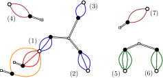
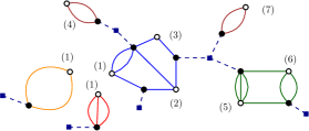
Figure 7: Left: the factorized map $(\gamma_{\lambda},\tau^{-1})$ and the blocks of $\pi$ (represented by the white squares and the colors). Right: the collection of non-separable hypermaps $(\nu,\tau)=\{({\gamma_{\lambda}}_{\lvert_{G}},\nu_{G})\}_{G\in\pi}$, together with a forest-like partition $\pi^{\prime\prime}$, whose blocks are indicated by the blue vertices.

Since $\Pi(\gamma_{\lambda})\geq\Pi(\tau)$, the condition $\pi^{\prime}\vee\Pi(\gamma_{\lambda})=1_{n}$ is translated as $\pi^{\prime\prime}\vee\Pi(\gamma_{\lambda})=1_{n}$. Conditionally to $L[\pi,\Pi(\gamma_{\lambda})\,;\,\Pi(\tau)]=0$, the following is true (where we recall that $\Pi(\tau)\vee\Pi(\nu)$):

$$\left\{\begin{array}[]{cc}L[\pi^{\prime\prime}\vee\Pi(\tau),\,\Pi(\gamma_{\lambda})\,;\,\Pi(\tau)]=0\\ L[\pi^{\prime\prime},\,\pi\,;\,\Pi(\nu)]=0\end{array}\right\}\qquad\Leftrightarrow\qquad L[\pi^{\prime\prime},\,\Pi(\gamma_{\lambda})\vee\Pi(\nu)\,;\,\Pi(\nu)]=0,$$ (4.22)

as:

$$L[\pi^{\prime\prime}\vee\Pi(\tau),\,\Pi(\gamma_{\lambda})\,;\,\Pi(\tau)]+L[\pi^{\prime\prime},\,\pi\,;\,\Pi(\nu)]=L[\pi^{\prime\prime},\,\Pi(\gamma_{\lambda})\vee\Pi(\nu)\,;\,\Pi(\nu)]+L[\pi,\Pi(\gamma_{\lambda})\,;\,\Pi(\tau)].$$

Therefore:

$$\beta_{\lambda_{1},\ldots,\lambda_{p}}=\sum_{\begin{subarray}{c}{\tau=\bigtimes_{i}\tau_{i}}\\[0.90417pt] {\tau_{i}\in\mathrm{NC}(\lambda_{i})}\end{subarray}}\ \sum_{\begin{subarray}{c}{\pi\geq\Pi(\tau)}\\[0.90417pt] {L[\pi,\Pi(\gamma_{\lambda})\,;\,\Pi(\tau)]=0}\end{subarray}}\ \sum_{\begin{subarray}{c}{\nu=\bigtimes_{G\in\pi}\nu_{G}}\\[0.90417pt] {\nu_{G}\in\mathrm{NS}(\tau_{\lvert_{G}})}\end{subarray}}\ \sum_{\begin{subarray}{c}{\pi^{\prime\prime}\geq\Pi(\nu)}\\[0.90417pt] {\pi^{\prime\prime}\vee\Pi(\gamma_{\lambda})=1_{n}}\\[0.90417pt] {L[\pi^{\prime\prime},\,\Pi(\gamma_{\lambda})\vee\Pi(\nu)\,;\,\Pi(\nu)]=0}\end{subarray}}f(\pi^{\prime\prime},\nu).$$ (4.23)

Consider a triplet $(\tau,\pi,\nu)$, where $\tau$ is a factorized planar bipartite map $\tau=\bigtimes_{i}\tau_{i}$, $\tau_{i}\in\mathrm{NC}(\lambda_{i})$; $\pi\geq\Pi(\tau)$ satisfies $L[\pi,\,\Pi(\gamma_{\lambda})\,;\,\Pi(\tau)]=0$, that is, it is a forest-like partition of the black vertices of the factorized map $(\gamma_{\lambda},\tau^{-1})$; and $\nu=\bigtimes_{G\in\pi}\nu_{G}$, where the $\nu_{G}\in\mathrm{NS}(\tau_{\lvert_{G}})$ are non-separable hypermaps, one for each block of $\pi$, so that in particular, $\pi=\Pi(\nu)\vee\Pi(\tau)$.

The permutation $\nu$ defines a non-necessarily-factorized planar bipartite map with $p$ white vertices $(\gamma_{\lambda},\nu)$. The partition $\pi\in\mathcal{P}(n)$ can then be read on $(\gamma_{\lambda},\nu)$: it is the partition of its edges given by the unique decomposition in non-separable hypermaps (see Sec. 2.4). This map can be seen as obtained gluing back the non-separable hypermaps on the right of Fig. 7 to the white vertices of the factorized map on the left of Fig. 7 (since each edge is an edge both around a white vertex of the factorized map and of a non-separable hypermap), obtaining the example of Fig. 8.

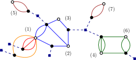
Figure 8: The generic planar map $(\gamma_{\lambda},\nu)$, together with the forest-like partition $\pi^{\prime\prime}$. The colors correspond to its decomposition in non-separable hypermaps.

A consequence of $\pi\geq\Pi(\tau)$, $L[\pi,\,\Pi(\gamma_{\lambda})\,;\,\Pi(\tau)]=0$ is that the restriction of $(\gamma_{\lambda},\tau^{-1})$ to a block $G\in\pi$ is a collection of disjoint planar bipartite maps with two vertices (bottom left of Fig. 6), that is, $\tau_{G}={\gamma_{\lambda}}_{\lvert_{G}}$. This means that the decomposition of $(\gamma_{\lambda},\nu)$ in non-separable hypermaps is $\{({\gamma_{\lambda}}_{\lvert_{G}},\nu_{G})\}_{G\in\pi}=(\tau,\nu)$. Consider a recursive splitting of edges of $(\gamma_{\lambda},\nu)$ leading to its terminal form $(\tau,\nu)$. At every splitting, the two corners belong to the same face and a new face is formed after the splitting. The total number of faces created is the difference between the number of connected components of $(\tau,\nu)$ and $(\gamma_{\lambda},\nu)$, so that:

$$\#(\nu\gamma_{\lambda})=\#(\nu\tau)+\#(\Pi(\nu)\vee\Pi(\gamma_{\lambda}))-\#(\Pi(\nu)\vee\Pi(\tau)).$$ (4.24)

From this, we see that

$$2g(\gamma_{\lambda},\nu) =2\#(\Pi(\nu)\vee\Pi(\gamma_{\lambda}))+n-\#(\nu)-\#(\gamma_{\lambda})-\#(\nu\gamma_{\lambda})$$

$$=2g(\nu,\tau)+L[\Pi(\nu)\vee\Pi(\tau),\,\Pi(\gamma_{\lambda})\,;\,\Pi(\tau)]$$

so that $g(\gamma_{\lambda},\nu)$ vanishes as long as $L[\pi,\,\Pi(\gamma_{\lambda})\,;\,\Pi(\tau)]=0$ and $g(\nu,\tau)=0$.

Reciprocally, given $\nu\in S_{n}$ which defines a generic planar bipartite map $g(\gamma_{\lambda},\nu)=0$, we decompose it into a triplet $(\tau,\pi,\nu)$ as follows: We consider its unique decomposition in non-separable hypermaps. It induces a partition $\pi\in\mathcal{P}(n)$ of the edges of the original map, which is such that or each block $G$ of this partition, the permutations ${\gamma_{\lambda}}_{\lvert_{G}}$ and $\nu_{G}$ respectively induced by ${\gamma_{\lambda}}$ and $\nu$ on $G$ satisfy $\nu_{G}\in\mathrm{NS}({\gamma_{\lambda}}_{\lvert_{G}})$. Letting $\gamma_{i}$ be the restriction of $\gamma_{\lambda}$ to $\{\sum_{j<i}\lambda_{j}+1,\ldots,\sum_{j<i}\lambda_{j}+\lambda_{i}\}$, we now set $\tau_{i}:=\bigtimes_{G\in\pi}{\gamma_{i}}_{\lvert_{G}}$. From the construction, $\pi\geq\Pi(\tau)$.

We have to justify that $L[\pi,\,\Pi(\gamma_{\lambda})\,;\,\Pi(\tau)]=0$: it is equivalent to the following incidence graph $\mathcal{G}$ being a forest: consider the white vertices of the map (the cycles of $\gamma_{\lambda}$), add a new black vertex for each non-separable hypermap component $G\in\pi$, and an edge between a black vertex and a white vertex whenever some of the edges around that white vertex belong to $G$ in $(\gamma_{\lambda},\nu^{-1})$. Consider a recursive splitting of edges of the map $(\gamma_{\lambda},\nu)$ leading to its decomposition in non-separable hypermaps. Each such step corresponds to the removal of an edge of $\mathcal{G}$, and the number of connected components are raised both in the map and the incidence graph. The terminal map whose connected components are the non-separable hypermap components of $(\gamma_{\lambda},\nu)$ corresponds to the terminal incidence graph which is just a collection of vertices with no edges. This shows that $\mathcal{G}$ is a forest.

Therefore, (4.23) is equivalent to

$$\beta_{\lambda_{1},\ldots,\lambda_{p}}=\sum_{\begin{subarray}{c}{\nu\in S_{n},}\\[0.90417pt] {g(\gamma_{\lambda},\nu)=0}\end{subarray}}\ \sum_{\begin{subarray}{c}{\pi^{\prime\prime}\geq\Pi(\nu)}\\[0.90417pt] {\pi^{\prime\prime}\vee\Pi(\gamma_{\lambda})=1_{n}}\\[0.90417pt] {L[\pi^{\prime\prime},\,\Pi(\gamma_{\lambda})\vee\Pi(\nu)\,;\,\Pi(\nu)]=0}\end{subarray}}f(\pi^{\prime\prime},\nu).$$

This indeed coincides with (4.5) by opting for the inverse of $\nu$. ∎

4.3 Corrections to the vertex weights for small orders

In this subsection, we take a closer look at the weight $g$ (4.8) associated to the blocks of the tree-like partition $\pi^{\prime}$ in Th. 4.2.

First order.

Consider (4.8). If $\tau_{\lvert_{B}}$ has one cycle of length $d$ only, then it is a cycle of one of the $\tau_{i}$, so that $I_{B}=\{i\}$, and $\bar{\pi}$ is the trivial partition of a single element, which is not an element of $\mathcal{P}^{*}(\{i\})$. In this case, there is no correction to $f$:

$$g(1_{d},\gamma_{d})=f(1_{d},\gamma_{d}).$$

4.3.1 Second order

If $\tau_{\lvert_{B}}$ has only two cycles respectively of lengths $m,n$, (4.8) is the trick of [9]. There are two contributions, and we can write (4.8) more simply as:

$$g(1_{m+n},\gamma_{m,n})=f(1_{m+n},\gamma_{m,n})+\sum_{\nu\in\mathrm{NS}(m,n)}f(\Pi(\nu),\nu).$$ (4.25)

Indeed, the two cycles of $\tau_{\lvert_{B}}$ must be respectively cycles of $\tau_{a}$ and $\tau_{b}$, $a<b$, and the sum over $\bar{\pi}$ in (4.8) has one term: the one-block partition $\bar{\pi}=\{a,b\}$, which is given by (4.10). Setting $f(1_{k_{1}+\cdots+k_{p}},\gamma_{k_{1},\ldots,k_{p}})=\kappa_{k_{1},\ldots,k_{p}}$, we have in terms of generating functions:

$$H_{2}(Y_{1},Y_{2})=C_{2}(Y_{1},Y_{2})+\tilde{C}_{2}(Y_{1},Y_{2}).$$ (4.26)

Letting

$$\tilde{\kappa}_{m,n}:=\sum_{\nu\in\mathrm{NS}(m,n)}\kappa(\Pi(\nu),\nu),$$ (4.27)

we see from (4.14) (see also the proof of Prop. 6.1 of [9]), that

$$\tilde{\kappa}_{m,n}=\sum_{r\geq 1}\sum_{\begin{subarray}{c}{i_{1},\ldots,i_{r}\geq 1}\\ {i_{1}+\cdots+i_{r}=m}\end{subarray}}\,\,\sum_{\begin{subarray}{c}{j_{1},\ldots,j_{r}\geq 1}\\ {j_{1}+\cdots+j_{r}=n}\end{subarray}}i_{1}n\ \prod_{s=1}^{r}\kappa_{i_{s}+j_{s}}.$$ (4.28)

Indeed, the elements of $\mathrm{NS}(m,n)$ consist of two white vertices $a<b$ and $r$ black vertices, $r\geq 1$, such that each black vertex is connected to both white vertices. Labelling the black edges as above (4.14), we consider the simpler notations $i_{s}:=j_{a,s}$ and $j_{s}=j_{b,s}$. The tree $T$ being trivial, we only have the bottom right contribution of (4.14) with $j_{G}^{s}=i_{s}+j_{s}$. The maps that have the same permutation for the white vertices and the same adjacency matrix differ only by the position of the edge with smallest label among the $i_{1}$ edges connecting $a$ and $1$, and the $n=\sum_{s}j_{s}$ ways to rotate the cycle $b$, so that $\mathcal{N}_{r}(\{i_{s},j_{s}\}_{s})=i_{1}n$.

This leads to the generating function (4.18):

$$\tilde{C}_{2}\bigl{(}Y_{1},Y_{2}\bigr{)}=\sum_{r\geq 1}Y_{2}\frac{\partial}{\partial Y_{2}}\Biggl{\{}\hat{C}(Y_{1},Y_{2})^{r-1}\,Y_{1}\frac{\partial}{\partial Y_{1}}\hat{C}(Y_{1},Y_{2})\Biggr{\}},$$

with $\hat{C}(Y_{1},Y_{2})=\sum_{i,j\geq 1}\kappa_{i+j}Y_{1}^{i}Y_{2}^{j}$, which are computed as:

$$\tilde{C}_{2}\bigl{(}Y_{1},Y_{2}\bigr{)}=-Y_{1}Y_{2}\frac{\partial}{\partial Y_{1}}\frac{\partial}{\partial Y_{2}}\log\bigl{(}1-\hat{C}(Y_{1},Y_{2})\bigr{)},$$ (4.29)

and:

$$\hat{C}(Y_{1},Y_{2})=1+\frac{Y_{1}}{Y_{2}-Y_{1}}C_{1}(Y_{2})+\frac{Y_{2}}{Y_{1}-Y_{2}}C_{1}(Y_{1}).$$ (4.30)

For $Y_{i}=X_{i}C_{1}(Y_{i})=X_{i}M_{1}(X_{i})$, this can be computed as:

$$\tilde{C}_{2}\bigl{(}Y_{1},Y_{2}\bigr{)}=\frac{Y_{1}Y_{2}}{(Y_{1}-Y_{2})^{2}}-\frac{Y_{1}Y_{2}}{(X_{1}-X_{2})^{2}}\frac{\mathrm{d}X_{1}}{\mathrm{d}Y_{1}}\frac{\mathrm{d}X_{2}}{\mathrm{d}Y_{2}},$$ (4.31)

and we recover the second-order relation (2.60).

4.3.2 Third order

Assuming now that $\tau_{\lvert_{B}}$ has only three disjoint cycles $\eta_{a}$, $\eta_{b}$, and $\eta_{c}$, respectively cycles of $\tau_{a}$, $\tau_{b}$, and $\tau_{c}$ for $a<b<c$, and respectively of lengths $l,m,n$, there are now three kinds of contributions to (4.8), illustrated in Fig. 9: that given by $f$, that given by $\tilde{f}$ (4.10) for $\bar{\pi}$ the one-block partition and $T$ the trivial tree, and the terms of the form (4.13) for $\bar{\pi}$ having two blocks and $T$ being the only element of $\mathcal{G}_{2}$. If $\bar{\pi}=\{a\}\{b,c\}$:

$$\bar{f}_{\{a\}\{b,c\}}(\tau_{\lvert_{B}})=\sum_{\begin{subarray}{c}{\nu=\eta_{i}\times\nu_{2}}\\[1.20552pt] {\nu_{2}\in\mathrm{NS}(\eta_{j}\times\eta_{k})}\end{subarray}}\ \sum_{F_{2}\in\Pi(\nu_{2})}\ f\Bigl{(}1_{l+\lvert F_{2}\rvert},\eta_{i}\times({\nu_{2}}_{\lvert_{F_{2}}})\Bigr{)}\prod_{\begin{subarray}{c}{V\in\Pi(\nu_{2})}\\ {V\notin F_{2}}\end{subarray}}f(1_{\lvert V\rvert},{\nu_{2}}_{\lvert_{V}}).$$ (4.32)

Setting $f(1_{k_{1}+\cdots+k_{p}},\gamma_{k_{1},\ldots,k_{p}})=\kappa_{k_{1},\ldots,k_{p}}$, we have in terms of generating functions:

$$H_{3}=C_{3}+\tilde{C}_{3}+\bar{C}_{3,\{1\}\{2,3\}}+\bar{C}_{3,\{1,2\}\{3\}}+\bar{C}_{3,\{2\}\{1,3\}}.$$ (4.33)

Figure 9: Contributions at third order. From left to right: $C_{3}$, $\tilde{C}_{3}$, $\bar{C}_{3,\{1\}\{2,3\}}$.

Proposition 4.3.

For the third order case, the corrections to $C_{3}$ in $H_{3}$ are the three terms given by (4.17) for $\#(\bar{\pi})=2$, of the form

$$\bar{C}_{3,\{1\}\{2,3\}}\bigl{(}Y_{1},Y_{2},Y_{3}\bigr{)}=Y_{2}Y_{3}\frac{\partial}{\partial Y_{2}}\frac{\partial}{\partial Y_{3}}\left[\frac{Y_{3}C_{2}(Y_{1},Y_{2})-Y_{2}C_{2}(Y_{1},Y_{3})}{Y_{2}C_{1}(Y_{3})-Y_{3}C_{1}(Y_{2})}\right],$$ (4.34)

and similarly for $\bar{\pi}=\{2\}\{1,3\}$ and $\bar{\pi}=\{3\}\{1,2\}$, and the remaining term $\tilde{C}_{3}$ (4.18) given by

$$\tilde{C}_{3}(Y_{1},Y_{2},Y_{3}) =Y_{1}Y_{2}Y_{3}\frac{\partial}{\partial Y_{1}}\frac{\partial}{\partial Y_{2}}\frac{\partial}{\partial Y_{3}}\Biggl{[}\frac{(1+\hat{C}(Y_{1},Y_{2},Y_{3}))^{2}+\hat{C}(Y_{1},Y_{2})\hat{C}(Y_{1},Y_{3})\hat{C}(Y_{2},Y_{3})-1}{(1-\hat{C}(Y_{1},Y_{2}))(1-\hat{C}(Y_{1},Y_{3}))(1-\hat{C}(Y_{2},Y_{3}))}$$

$$\hskip 142.26378pt+\sum_{\begin{subarray}{c}{1\leftrightarrow 2}\\ {1\leftrightarrow 3}\end{subarray}}\frac{Y_{1}^{2}\frac{\partial}{\partial Y_{1}}\left(\frac{1}{Y_{1}}\hat{C}(Y_{1},Y_{2},Y_{3})\right)}{(1-\hat{C}(Y_{1},Y_{2}))(1-\hat{C}(Y_{1},Y_{3}))}\Biggr{]},$$ (4.35)

where $\hat{C}$ was defined in (4.30), and:

$$\hat{C}(Y_{1},Y_{2},Y_{3})=\frac{Y_{3}}{Y_{2}-Y_{3}}\hat{C}(Y_{1},Y_{2})+\frac{Y_{2}}{Y_{3}-Y_{2}}\hat{C}(Y_{1},Y_{3}).$$ (4.36)

With this and from Thm. 4.1 and Thm. 4.2, we have all the ingredients of the third-order moment-cumulant relation.

Proof.

From (4.14), the expression for $\bar{\kappa}_{\{1\}\{2,3\}}(\gamma_{l,m,n})$ is very similar to that of $\tilde{\kappa}_{m,n}$ in (4.28), with the difference that a cycle $\theta\in\{1,\ldots,r\}$ of $\nu_{2}\in\mathrm{NS}(m,n)$ is chosen, for which the term $\kappa_{i_{\theta}+j_{\theta}}$ is replaced by the second order free cumulant $\kappa_{l,i_{\theta}+j_{\theta}}$:

$$\bar{\kappa}_{\{1\}\{2,3\}}(\gamma_{l,m,n})=\sum_{r\geq 1}\sum_{\begin{subarray}{c}{i_{1},\ldots,i_{r}\geq 1}\\ {i_{1}+\cdots+i_{r}=m}\end{subarray}}\,\,\sum_{\begin{subarray}{c}{j_{1},\ldots,j_{r}\geq 1}\\ {j_{1}+\cdots+j_{r}=n}\end{subarray}}\sum_{\theta=1}^{r}i_{1}n\,\kappa_{i_{1}+j_{1}}\ldots\kappa_{l,i_{\theta}+j_{\theta}}\ldots\kappa_{i_{r}+j_{r}}.$$ (4.37)

The generating function for these numbers is found to be

$$\bar{C}_{3,\{1\}\{2,3\}}\bigl{(}Y_{1},Y_{2},Y_{3}\bigr{)} =\sum_{l,m,n\geq 1}\bar{\kappa}_{\{1\}\{2,3\}}(\gamma_{l,m,n})Y_{1}^{l}Y_{2}^{m}Y_{3}^{n}$$ (4.38)

$$=\sum_{r\geq 1}Y_{2}Y_{3}\frac{\partial}{\partial Y_{2}}\frac{\partial}{\partial Y_{3}}\Biggl{\{}\hat{C}(Y_{2},Y_{3})^{r-1}\sum_{l,i,j\geq 1}\kappa_{l,i+j}Y_{1}^{l}Y_{2}^{i}Y_{3}^{j}\Biggr{\}}$$ (4.39)

$$=Y_{2}Y_{3}\frac{\partial}{\partial Y_{2}}\frac{\partial}{\partial Y_{3}}\Biggl{\{}\frac{1}{1-\hat{C}(Y_{2},Y_{3})}\hat{C}_{\{1\}\{2,3\}}(Y_{1},Y_{2},Y_{3})\Biggr{\}},$$ (4.40)

where $\hat{C}_{\{1\}\{2,3\}}(Y_{1},Y_{2},Y_{3})=\sum_{l,i,j\geq 1}\kappa_{l,i+j}Y_{1}^{l}Y_{2}^{i}Y_{3}^{j}$ is computed as:

$$\bigl{(}Y_{2}-Y_{3}\bigr{)}\hat{C}_{\{1\}\{2,3\}}(Y_{1},Y_{2},Y_{3})=Y_{3}C_{2}(Y_{1},Y_{2})-Y_{2}C_{2}(Y_{1},Y_{3}),$$ (4.41)

which concludes the proof of (4.34).

We now turn to $\tilde{C}_{3}$ (4.18), the generating function of non-separable hypermaps with white vertices given by $\gamma_{l,m,n}$, whose hyper-edges are weighted by first-order free cumulants:

$$\tilde{C}_{3}\bigl{(}Y_{1},Y_{2},Y_{3}\bigr{)}=\sum_{s,m,n}Y_{1}^{s}Y_{2}^{m}Y_{3}^{n}\sum_{\nu\in\mathrm{NS}(s,m,n)}\ \kappa(\Pi(\nu),\nu).$$ (4.42)

There are three kinds of contributions, illustrated in Fig. 10.

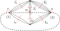
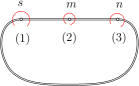
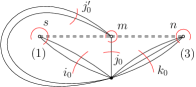
Figure 10: Non-separable hypermaps with three white vertices. The thick dotted edges represent non-separable hypermaps with two white vertices. In the case where these thick edges are dotted, these hypermaps may be absent. The black vertices (and incident edges) on the left diagram may be absent or not, but there must be at least one.

The case where both back vertices are present contributes as:

$$smn\sum_{\begin{subarray}{c}{i_{0},j_{0},k_{0}\geq 1}\\ {i_{0}^{\prime},j_{0}^{\prime},k_{0}^{\prime}\geq 1}\end{subarray}}\ \sum_{r_{12},r_{13},r_{23}\geq 0}\ \sum_{\begin{subarray}{c}{\{i_{a}\}_{1\leq a\leq r_{12}},\{i_{a}^{\prime}\}_{1\leq a\leq r_{13}}}\\ {\sum i_{a}+\sum i_{a}^{\prime}+i_{0}+i_{0}^{\prime}=s}\end{subarray}}\sum_{\begin{subarray}{c}{\{j_{a}\}_{1\leq a\leq r_{12}},\{j_{a}^{\prime}\}_{1\leq a\leq r_{23}}}\\ {\sum j_{a}+\sum j_{a}^{\prime}+j_{0}+j_{0}^{\prime}=m}\end{subarray}}\sum_{\begin{subarray}{c}{\{k_{a}\}_{1\leq a\leq r_{23}},\{k_{a}^{\prime}\}_{1\leq a\leq r_{13}}}\\ {\sum k_{a}+\sum k_{a}^{\prime}+k_{0}+k_{0}^{\prime}=n}\end{subarray}}$$

$$\prod_{a=1}^{r_{12}}\kappa_{i_{a}+j_{a}}\prod_{a=1}^{r_{13}}\kappa_{i_{a}^{\prime}+k_{a}^{\prime}}\prod_{a=1}^{r_{23}}\kappa_{j_{a}^{\prime}+k_{a}}\kappa_{i_{0}+j_{0}+k_{0}}\kappa_{i^{\prime}_{0}+j^{\prime}_{0}+k^{\prime}_{0}},$$ (4.43)

where the factor $smn$ comes from rotating the cycles of $\gamma_{s,m,n}$ for each white vertex (choosing which edge is its smallest element). This leads to the generating function:

$$Y_{1}Y_{2}Y_{3}\frac{\partial}{\partial Y_{1}}\frac{\partial}{\partial Y_{2}}\frac{\partial}{\partial Y_{3}}\Biggl{[}\frac{\hat{C}(Y_{1},Y_{2},Y_{3})^{2}}{(1-\hat{C}(Y_{1},Y_{2}))(1-\hat{C}(Y_{1},Y_{3}))(1-\hat{C}(Y_{2},Y_{3}))}\Biggr{]},$$

where $\hat{C}(Y_{1},Y_{2},Y_{3})=\sum_{i,j,k\geq 1}\kappa_{i+j+k}Y_{1}^{l}Y_{2}^{i}Y_{3}^{j}$ is computed as:

$$\bigl{(}Y_{2}-Y_{3}\bigr{)}\hat{C}(Y_{1},Y_{2},Y_{3})=Y_{3}\hat{C}(Y_{1},Y_{2})-Y_{2}\hat{C}(Y_{1},Y_{3}).$$ (4.44)

The contributions when a single black vertex is present is given by

$$Y_{1}Y_{2}Y_{3}\frac{\partial}{\partial Y_{1}}\frac{\partial}{\partial Y_{2}}\frac{\partial}{\partial Y_{3}}\Biggl{[}\frac{2\hat{C}(Y_{1},Y_{2},Y_{3})}{(1-\hat{C}(Y_{1},Y_{2}))(1-\hat{C}(Y_{1},Y_{3}))(1-\hat{C}(Y_{2},Y_{3}))}\Biggr{]},$$

and the contribution to the diagram in the middle of Fig. 10 by

$$Y_{1}Y_{2}Y_{3}\frac{\partial}{\partial Y_{1}}\frac{\partial}{\partial Y_{2}}\frac{\partial}{\partial Y_{3}}\Biggl{[}\frac{C(Y_{1},Y_{2})}{(1-\hat{C}(Y_{1},Y_{2}))}\frac{C(Y_{1},Y_{3})}{(1-\hat{C}(Y_{1},Y_{3}))}\frac{C(Y_{2},Y_{3})}{(1-\hat{C}(Y_{2},Y_{3}))}\Biggr{]}.$$

The right diagram contributes as

$$smn\sum_{\begin{subarray}{c}{i_{0},j_{0},i_{0}^{\prime}\geq 1}\end{subarray}}\ \sum_{r_{12},r_{23}\geq 0}\ \sum_{\begin{subarray}{c}{\{i_{a}\}_{1\leq a\leq r_{12}}}\\ {\sum i_{a}+i_{0}=s}\end{subarray}}\sum_{\begin{subarray}{c}{\{j_{a}\}_{1\leq a\leq r_{12}},\{j_{a}^{\prime}\}_{1\leq a\leq r_{23}}}\\ {\sum j_{a}+\sum j_{a}^{\prime}+j_{0}+j_{0}^{\prime}=m}\end{subarray}}\sum_{\begin{subarray}{c}{\{k_{a}\}_{1\leq a\leq r_{23}}}\\ {\sum k_{a}+k_{0}=n}\end{subarray}}$$

$$\hskip 199.16928pt\prod_{a=1}^{r_{12}}\kappa_{i_{a}+j_{a}}\prod_{a=1}^{r_{23}}\kappa_{j_{a}^{\prime}+k_{a}}\kappa_{i_{0}+j_{0}+j_{0}^{\prime}+k_{0}},$$ (4.45)

leading to the generating function

$$Y_{1}Y_{2}Y_{3}\frac{\partial}{\partial Y_{1}}\frac{\partial}{\partial Y_{2}}\frac{\partial}{\partial Y_{3}}\Biggl{[}\frac{\sum_{i,j,j^{\prime},k\geq 1}\kappa_{i+j+j^{\prime}+k}Y_{1}^{i}Y_{2}^{j+j^{\prime}}Y_{3}^{k}}{(1-\hat{C}(Y_{1},Y_{2}))(1-\hat{C}(Y_{2},Y_{3}))}\Biggr{]},$$

and we compute:

$$\sum_{i,j,j^{\prime},k\geq 1}\kappa_{i+j+j^{\prime}+k}Y_{1}^{i}Y_{2}^{j+j^{\prime}}Y_{3}^{k}=\sum_{i,j,k\geq 1}(p-1)\kappa_{i+j+k}Y_{1}^{i}Y_{2}^{j}Y_{3}^{k}=Y_{2}\frac{\partial}{\partial Y_{2}}\hat{C}(Y_{1},Y_{2},Y_{3})-\hat{C}(Y_{1},Y_{2},Y_{3}).$$

This concludes the proof of (4.35). ∎

Remark.

One may alternatively compute $\tilde{C}_{3}$ as

$$\tilde{C}_{3}(Y_{1},Y_{2},Y_{3}) =Y_{1}Y_{3}\frac{\partial}{\partial Y_{1}}\frac{\partial}{\partial Y_{3}}\left(\frac{Y_{3}\tilde{C}_{2}(Y_{1},Y_{2})-Y_{1}\tilde{C}_{2}(Y_{2},Y_{3})}{Y_{1}C_{1}(Y_{3})-Y_{3}C_{1}(Y_{1})}\right)$$ (4.46)

$$+Y_{1}Y_{2}Y_{3}\frac{\partial}{\partial Y_{1}}\frac{\partial}{\partial Y_{2}}\frac{\partial}{\partial Y_{3}}\left[\frac{Y_{2}^{2}\frac{\partial}{\partial Y_{2}}\left(\frac{1}{Y_{2}}\hat{C}(Y_{1},Y_{2},Y_{3})\right)-\hat{C}(Y_{1},Y_{2})\hat{C}(Y_{2},Y_{3})}{(1-\hat{C}(Y_{1},Y_{2}))(1-\hat{C}(Y_{2},Y_{3}))}\right],$$

In a similar way as above, recalling the definition of $\tilde{\kappa}_{i,j}$ in (4.27), one finds that the following series

$$\sum_{r\geq 1}\sum_{\begin{subarray}{c}{i_{1},\ldots,i_{r}\geq 1}\\ {i_{1}+\cdots+i_{r}=s}\end{subarray}}\,\,\sum_{\begin{subarray}{c}{j_{1},\ldots,j_{r}\geq 1}\\ {j_{1}+\cdots+j_{r}=n}\end{subarray}}\sum_{\theta=1}^{r}i_{1}n\,\kappa_{i_{1}+j_{1}}\ldots\tilde{\kappa}_{m,i_{\theta}+j_{\theta}}\ldots\kappa_{i_{r}+j_{r}},$$ (4.47)

generates exactly once the major part of the elements of $\mathrm{NS}(s,m,n)$, with the exception of the terms for the diagram on the right of Fig. 10, which we have to add, and which we have computed above. It also generates elements as in the middle of Fig. 10 but without the thick line linking 1 and 3, which are not in $\mathrm{NS}(s,m,n)$, and which we have to substract. The series (4.47) is similar to what we have detailed above and provides the contribution in the first line of (4.35). The terms to be substracted are generated by:

$$Y_{1}Y_{2}Y_{3}\frac{\partial}{\partial Y_{1}}\frac{\partial}{\partial Y_{2}}\frac{\partial}{\partial Y_{3}}\left(\frac{\hat{C}(Y_{1},Y_{2})}{(1-\hat{C}(Y_{1},Y_{2}))}\frac{\hat{C}(Y_{2},Y_{3})}{(1-\hat{C}(Y_{2},Y_{3}))}\right).$$ (4.48)

4.3.3 Fourth order

Consider $\tau_{\lvert_{B}}$ with four disjoint cycles $\eta_{a}$, $\eta_{b}$, $\eta_{c}$ and $\eta_{d}$, respectively cycles of $\tau_{a}$, $\tau_{b}$, $\tau_{c}$ $\tau_{d}$ for $a<b<c<d$, and respectively of lengths $l,m,n,q$, there are now six kinds of contributions to (4.8), illustrated in Fig. 11: that given by $f$; that given by $\tilde{f}$ (4.10) for $\bar{\pi}$ the one-block partition and $T$ the trivial tree; two kinds of terms of the form (4.13) for $\bar{\pi}$ having two blocks and $T$ being the only element of $\mathcal{G}_{2}$: one for $\bar{\pi}$ having blocks with 1 and 3 elements, the other with 2 and 2 element; and finally two kinds of terms for $\bar{\pi}$ with three blocks: one of the form (4.13) for $T$ with a single blue vertex, and the one where $T$ has two blue vertices.

$$H_{4}=C_{4}+\tilde{C}_{4}+\sum_{\mathrm{perm}}\bar{C}_{4,\{1\}\{2,3,4\}}+\sum_{\mathrm{perm}}\bar{C}_{4,\{1,2\}\{3,4\}}+\sum_{\mathrm{perm}}\bar{C}_{4,\{1\}\{2\}\{3,4\}}+\sum_{\mathrm{perm}}\bar{C}_{4,\{1\}\{2\}\{3,4\},T},$$ (4.49)

where the sums are over appropriate permutations of the indices.

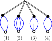
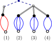
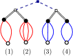
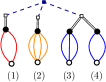
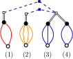
Figure 11: Corrections at fourth order. From left to right: $\tilde{C}_{4}$, $\bar{C}_{4,\{1\}\{2,3,4\}}$, $\bar{C}_{4,\{1,2\}\{3,4\}}$, $\bar{C}_{4,\{1\}\{2\}\{3,4\}}$, and $\bar{C}_{4,\{1\}\{2\}\{3,4\},T}$ for $T$ with two blue vertices.

Here we only compute $C_{4,\{1,2\}\{3,4\}}$ and $\bar{C}_{4,\{1\}\{2\}\{3,4\},T}$. $\bar{C}_{4,\{1\}\{2\}\{3,4\}}$ will be computed in (5.11) as the particular case of $\bar{C}_{p,\bar{\pi}}$ for $\bar{\pi}$ having only one non-trivial block with two elements, see also Prop. 5.6. $\bar{C}_{4,\{1\}\{2,3,4\}}$ can be computed from the expression of $\tilde{C}_{3}$ above, but we will instead compute it in (5.53) after deriving a simpler expression for $\tilde{C}_{3}$ in Prop. 5.5, to avoid a three-lines-equation. Computing $\tilde{C}_{4}$ as we did for $\tilde{C}_{3}$ is painful and a more efficient approach should be prefered.

Proposition 4.4.

The following corrections can be easily computed:

$$\bar{C}_{4,\{1\},\{2\}\{3,4\},T}(Y_{1},Y_{2},Y_{3},Y_{4})=Y_{3}Y_{4}\frac{\partial}{\partial Y_{3}}\frac{\partial}{\partial Y_{4}}\left[\frac{\hat{C}_{\{1\}\{3,4\}}(Y_{1},Y_{3},Y_{4})\hat{C}_{\{2\}\{3,4\}}(Y_{2},Y_{3},Y_{4})}{(1-\hat{C}(Y_{3},Y_{4}))^{2}}\right],$$ (4.50)

where $T$ has two blue vertices and $\hat{C}_{\{a\}\{b,c\}}$ is given in (4.41), and:

$$\bar{C}_{4,\{1,2\}\{3,4\}}(Y_{1},Y_{2},Y_{3},Y_{4})=\left(\prod_{i=1}^{4}Y_{i}\frac{\partial}{\partial Y_{i}}\right)\left[\frac{\hat{C}_{\{1,2\}\{3,4\}}(Y_{1},Y_{2},Y_{3},Y_{4})}{(1-\hat{C}(Y_{1},Y_{2}))(1-\hat{C}(Y_{3},Y_{4})}\right],$$ (4.51)

where

$$\hat{C}_{\{1,2\}\{3,4\}}(Y_{1},Y_{2},Y_{3},Y_{4}) =\frac{Y_{2}}{Y_{1}-Y_{2}}\frac{Y_{4}}{Y_{3}-Y_{4}}C_{2}(Y_{1},Y_{3})+\frac{Y_{2}}{Y_{1}-Y_{2}}\frac{Y_{3}}{Y_{4}-Y_{3}}C_{2}(Y_{1},Y_{4})$$ (4.52)

$$\hskip 56.9055pt+\frac{Y_{1}}{Y_{2}-Y_{1}}\frac{Y_{4}}{Y_{3}-Y_{4}}C_{2}(Y_{2},Y_{3})+\frac{Y_{1}}{Y_{2}-Y_{1}}\frac{Y_{3}}{Y_{4}-Y_{3}}C_{2}(Y_{2},Y_{4}).$$

Proof.

From (4.14), the expression (4.9) for $\bar{\kappa}_{\{1\}\{2\}\{3,4\},T}(\gamma_{m_{1},n_{1},m_{2},n_{2}})$ is very similar to (4.37), with the difference that two edges of the tree must be attributed to black vertices of the non-separable hypermap defined by $\nu\in\mathrm{NS}(m_{2},n_{2})$:

$$\bar{\kappa}_{\{1,2\}\{3,4\}}(\gamma_{m_{1},n_{1},m_{2},n_{2}}) =\sum_{r\geq 2}\sum_{\begin{subarray}{c}{i_{1},\ldots,i_{r}\geq 1}\\ {i_{1}+\cdots+i_{r}=m_{2}}\end{subarray}}\,\,\sum_{\begin{subarray}{c}{j_{1},\ldots,j_{r}\geq 1}\\ {j_{1}+\cdots+j_{r}=n_{2}}\end{subarray}}\sum_{\theta_{1}\neq\theta_{2}=1}^{r}i_{1}n\,\kappa_{i_{1}+j_{1}}$$

$$\hskip 113.81102pt\ldots\kappa_{m_{1},i_{\theta_{1}}+j_{\theta_{1}}}\ldots\kappa_{n_{1},i_{\theta_{2}}+j_{\theta_{2}}}\ldots\kappa_{i_{r}+j_{r}},$$

The generating function is found to be:

$$\bar{C}_{4,\{1\},\{2\}\{3,4\},T}=Y_{3}Y_{4}\frac{\partial}{\partial Y_{3}}\frac{\partial}{\partial Y_{4}}\left[\hat{C}_{\{1\}\{3,4\}}(Y_{1},Y_{3},Y_{4})\hat{C}_{\{2\}\{3,4\}}(Y_{2},Y_{3},Y_{4})\sum_{r\geq 2}(r-1)\hat{C}(Y_{3},Y_{4})^{r-2}\right],$$

which is summed to (4.50).

The expression (4.9) for $\bar{\kappa}_{\{1,2\}\{3,4\}}(\gamma_{m_{1},n_{1},m_{2},n_{2}})$ is as (4.37), but now two summations over $\nu_{1}\in\mathrm{NS}(m_{1},n_{1})$ and $\nu_{2}\in\mathrm{NS}(m_{2},n_{2})$, and two cycles are chosen, a cycle $\theta_{1}$ of $\nu_{1}$ and one $\theta_{2}$ of $\nu_{2}$, for which the product of first order free cumulants is replaced by a second order free cumulant. This leads to:

$$\bar{\kappa}_{\{1,2\}\{3,4\}}(\gamma_{m_{1},n_{1},m_{2},n_{2}}) =\prod_{s=1,2}\Biggl{(}\sum_{r_{s}\geq 1}\sum_{\begin{subarray}{c}{i^{s}_{1},\ldots,i^{s}_{r_{s}}\geq 1}\\ {i^{s}_{1}+\cdots+i^{s}_{r_{s}}=m_{s}}\end{subarray}}\,\,\sum_{\begin{subarray}{c}{j^{s}_{1},\ldots,j^{s}_{r_{s}}\geq 1}\\ {j^{s}_{1}+\cdots+j^{s}_{r}=n_{s}}\end{subarray}}\sum_{\theta_{s}=1}^{r_{s}}\Biggr{)}$$ (4.53)

$$\hskip 85.35826pt\times i^{1}_{1}i^{2}_{1}n_{1}n_{2}\prod_{s=1,2}\prod_{\begin{subarray}{c}{1\leq a_{s}\leq r_{s}}\\ {a_{s}\neq\theta_{s}}\end{subarray}}\kappa_{i^{s}_{a}+j_{a}^{s}}\times\kappa_{i^{1}_{\theta_{1}}+j^{1}_{\theta_{1}},i^{2}_{\theta_{2}}+j^{2}_{\theta_{2}}}.$$ (4.54)

The generating function for these numbers is therefore found to be (4.51), where

$$\hat{C}_{\{1,2\}\{3,4\}}(Y_{1},Y_{2},Y_{3},Y_{4})=\sum_{i,j,k,l\geq 1}\kappa_{i+j,k+l}Y_{1}^{i}Y_{2}^{j}Y_{3}^{k}Y_{4}^{l}.$$ (4.55)

As for (4.41), this is computed as:

$$\bigl{(}Y_{1}-Y_{2}\bigr{)}\hat{C}_{\{1,2\}\{3,4\}}(Y_{1},Y_{2},Y_{3},Y_{4})=Y_{2}\hat{C}_{\{1\}\{3,4\}}(Y_{1},Y_{3},Y_{4})-Y_{1}\hat{C}_{\{2\}\{3,4\}}(Y_{2},Y_{3},Y_{4}),$$ (4.56)

which leads to (4.52). ∎

5 Efficient treatment of the corrections, simplifications

5.1 Corrections for several-blocks partitions

For $I\subset\{1,\ldots,p\}$, the corrections to $C_{\lvert I\rvert}$ in $H_{\lvert I\rvert}$ (4.15) are of the form $\bar{C}_{\lvert I\rvert,\bar{\pi},T}$ (4.16) for $\bar{\pi}\in\mathcal{P}^{\star}(I)$ and $T\in\mathcal{G}_{\bar{\pi}}$. The correction $\bar{C}_{\lvert I\rvert,\bar{\pi},T}$ simplifies to $\bar{C}_{\lvert I\rvert,\bar{\pi}}$ (4.17) if the tree $T$ has a single blue vertex, and to $\tilde{C}_{\lvert I\rvert}$ if $\bar{\pi}$ is the one-block partition $\bar{\pi}=\{I\}$. We have already computed three of the several-block corrections ($\bar{C}_{3,\{1\}\{2,3\}}$, $\bar{C}_{4,\{1,2\}\{3,4\}}$ and $\bar{C}_{4,\{1\},\{2\}\{3,4\},T}$), and at the level of the coefficients $\bar{\kappa}_{\bar{\pi},T}$ (4.14), the picture is a bit more clear, and it would be good to make these computations more efficient (and less repetitive) by working directly with the generating functions.

The picture of (4.14) is the following: to each pair $(G,K)$ where $G,K$ are respectively a white and a blue vertex of the tree $T$ corresponds an edge of $T$. For each such edge, a choice is made of one of the first order free cumulants from the expansions of the $\tilde{C}_{\lvert G\rvert}$ (this choice corresponds to $\theta({G,K})$ in (4.14)). For each $K$, the cumulants for the edges $(G,K)$ incident to $K$ are replaced by a higher order cumulant. In this subsection, we explain how these computations can be performed at the level of generating functions instead of coefficients, thus showing how all the corrections $\bar{C}_{\lvert I\rvert,\bar{\pi},T}$ can be computed efficiently by acting directly on the generating function $\tilde{C}_{\lvert I\rvert}$ of planar non-separable hyper-maps with weighted hyperedges (the one-block correction).

5.1.1 Trees with a single blue vertex

We consider $\mathbb{K}$, the set of formal power series in the first order free cumulants $1\cup\{\prod_{a}\kappa_{i_{a}}\}_{\{i_{a}>0\}}$,

$$c_{0}+\sum_{q}\sum_{i_{1},\ldots,i_{q}\geq 1}c_{i_{1},\ldots,i_{q}}\,\kappa_{i_{1}}\cdots\kappa_{i_{q}}$$

where the sum over $q$ has a finite support, whose coefficients $c_{0}$ and $c_{i_{1},\ldots,i_{q}}$ are themselves some formal power series in a set of variables $\{Y_{i}\}$ with complex coefficients (that may include higher order free cumulants). For a typical example in ${\mathbb{K}}_{2}$: $\sum_{i_{1},i_{2}\geq 0}\Bigl{(}\sum_{j_{1},j_{2}\geq 1}j_{1}\kappa_{j_{1},j_{2}+i_{2}}Y_{1}^{i_{i}+j_{1}}Y_{2}^{j_{2}}\Bigr{)}\kappa_{i_{1}}\kappa_{i_{2}},$ where $\kappa_{0}=1$. We define an operator by its action on the $\{\kappa_{i}\}_{i\geq 0}$:

$$\mathcal{D}:(\kappa_{i_{1}},\ldots,\kappa_{i_{d}})\mapsto\left\{\begin{array}[]{rcl}\textrm{if }\forall a,\,i_{a}>0&:&\kappa_{i_{1},\ldots,i_{d}}\\ \textrm{otherwise }&:&0\end{array}\right..$$ (5.1)

The $\kappa$ being symmetric in their arguments, $\mathcal{D}$ is symmetric too. We extend the definition of $\mathcal{D}$ to $\mathbb{K}^{d}$ by requiring the following:

• $\mathcal{D}$ is multilinear: let $\{V^{1}_{i_{1}},\ldots,V^{d}_{i_{d}}\}_{\{i_{a}\}}$ and $\{P^{1}_{i_{1}},\ldots,P^{d}_{i_{d}}\}_{\{i_{a}\}}$ such that for any $a,i_{a}$, $V^{a}_{i_{a}}\in\mathbb{K}$, and $P^{a}_{i_{a}}$ is some formal series in the $\{Y_{i}\}$ that does not involve first order free cumulants:

  $$\mathcal{D}\Bigl{(}\sum_{i_{1}\geq 0}P^{1}_{i_{1}}V^{1}_{i_{1}},\ldots,\sum_{i_{d}\geq 0}P^{d}_{i_{d}}V^{d}_{i_{d}}\Bigr{)}=\sum_{i_{1}\geq 0}P^{1}_{i_{1}}\cdots\sum_{i_{d}\geq 0}P^{d}_{i_{d}}\,\mathcal{D}(V^{1}_{i_{1}},\ldots,V^{d}_{i_{d}}).$$ (5.2)

• $\mathcal{D}$ satisfies a Leibniz rule on each one of its arguments, that is, considering $F_{1},F_{2}\in\bar{\mathbb{F}}$:

  $$\mathcal{D}(F_{1}F_{2},\ldots)=F_{1}\mathcal{D}(F_{2},\ldots)+F_{2}\mathcal{D}(F_{1},\ldots).$$

In other words, $\mathcal{D}$ is a multilinear partial differential form (since the higher order free cumulants are seen as coefficients) acting on the first order free cumulants as variables and considering any polynomial in the $Ys$ as constant (including higher order free cumulants). From the rules above, we find that if $F_{1},\ldots,F_{d}\in\bar{\mathbb{F}}$:

$$\frac{\partial}{\partial Y_{i}}\mathcal{D}(F_{1},\ldots,F_{d})=\sum_{a=1}^{d}\mathcal{D}\Bigl{(}F_{1},\ldots,\frac{\partial F_{a}}{\partial Y_{i}},\ldots,F_{d}\Bigr{)}.$$ (5.3)

If different arguments of $\mathcal{D}$ involve different variables $Y_{i}$, ${\partial}/{\partial Y_{i}}$ commutes with $\mathcal{D}$.

From the Leibniz rule, $\mathcal{D}$ satisfies the chain rule on each argument, that is, if for instance $F_{1}(X)=\sum_{k}c_{k}X^{k}$ and $H_{1}\in\mathbb{K}$, then $\mathcal{D}\bigl{(}F_{1}(H_{1}),\ldots\bigr{)}=F_{1}^{\prime}(H_{1})\mathcal{D}\,\bigl{(}H_{1},\ldots\bigr{)}$, and if $F_{1}(X_{1},\ldots,X_{q})=\sum_{k}c_{k_{1},\ldots,k_{q}}X_{1}^{k_{1}}\cdots X_{q}^{k_{q}}$, then:

$$\mathcal{D}\bigl{(}F_{1}(H_{1},\ldots,H_{q}),\ldots\bigr{)}=\sum_{\theta=1}^{q}\frac{\partial F_{1}}{\partial X_{\theta}}(H_{1},\ldots,H_{q})\ \mathcal{D}\bigl{(}H_{\theta},\ldots\bigr{)}.$$ (5.4)

In practice, we will use $\mathcal{D}$ through its action on $C_{1}$ as follows:

$$\mathcal{D}\bigl{(}C_{1}(Y_{1}),\ldots,C_{1}(Y_{d})\bigr{)}=C_{d}(Y_{1},\ldots,Y_{d}),$$ (5.5)

and applied to functions of the $C_{1}(Y_{i})$.

Lemma 5.1.

For $I\subset\{1,\ldots,p\}$ and $\bar{\pi}\in\mathcal{P}^{\star}(I)$, the several-blocks corrections $\bar{C}_{\lvert I\rvert,\bar{\pi}}$ can be derived from the one-block corrections $\tilde{C}_{\lvert B\rvert}$ for the $B\in\bar{\pi}$ (with $\tilde{C}_{1}=C_{1}$) as:

$$\bar{C}_{\lvert I\rvert,\bar{\pi}}\bigl{(}Y_{I}\bigr{)}=\mathcal{D}\Bigl{(}\{\tilde{C}_{\lvert B\rvert}(Y_{B})\}_{B\in\bar{\pi}}\Bigr{)}.$$ (5.6)

Proof.

This is seen directly on (4.17). With the same notations:

$$\kappa_{\{\lvert F_{G}\rvert\}_{G\in\bar{\pi}}}[b]=\mathcal{D}\Bigl{(}\{\kappa_{\lvert F_{G}\rvert}\}_{G\in\bar{\pi}}\Bigr{)},$$ (5.7)

so that since the Leibniz rule holds for each argument:

$$\sum_{\{F_{G}\in\Pi(\nu_{G})\}_{G\in\bar{\pi}}}\kappa_{\{\lvert F_{G}\rvert\}_{G\in\bar{\pi}}}\prod_{\begin{subarray}{c}{V\in\Pi(\bigtimes_{G}\nu_{G})}\\ {V\notin\{F_{G}\}}\end{subarray}}\kappa_{\lvert V\rvert}=\mathcal{D}\Bigl{(}\Bigl{\{}\kappa\bigl{(}\Pi(\nu_{G}),\nu_{G}\bigr{)}\Bigr{\}}_{G\in\bar{\pi}}\Bigr{)}.$$ (5.8)

By multilinearity:

$$\bar{C}_{\lvert I\rvert,\bar{\pi}}\bigl{(}\{Y_{i}\}_{i\in I}\bigr{)}=\mathcal{D}\Biggl{(}\Biggl{\{}\sum_{\{\mu_{i}\}_{i\in G}}\ \prod_{i\in G}Y_{i}^{\mu_{i}}\ \Bigl{[}\sum_{\nu_{G}\in\mathrm{NS}(\mu_{G})}\kappa\bigl{(}\Pi(\nu_{G}),\nu_{G}\bigr{)}\Bigr{]}\Biggr{\}}_{G\in\bar{\pi}}\Biggr{)},$$ (5.9)

where we recognize (4.18). ∎

This provides a more efficient way of computing the corrections $\bar{C}_{\lvert I\rvert,\bar{\pi}}$ from known $\tilde{C}_{p}$. For instance, let $\bar{C}_{p,\{a,b\}}$ be $\bar{C}_{p,\bar{\pi}},$ for $\bar{\pi}$ the partition of $\{1,\ldots,p\}$ whose blocks all contain a single element, apart from the block $\{a,b\}$. $\bar{C}_{p,\{a,b\}}$ can be computed from the coefficients as $\bar{C}_{3,\{1\}\{2,3\}}$, but applying Prop. 5.1, we find that

$$\bar{C}_{p,\{a,b\}}\bigl{(}Y_{1},\ldots,Y_{p}\bigr{)}=\mathcal{D}\Bigl{(}\tilde{C}_{2}(Y_{a},Y_{b}),\{C_{1}(Y_{i})\}_{i\neq a,b}\Bigr{)}.$$ (5.10)

Using the expression of $\tilde{C}_{2}$ in (4.29):

$$\bar{C}_{p,\{a,b\}}\bigl{(}Y_{1},\ldots,Y_{p}\bigr{)}=Y_{a}Y_{b}\frac{\partial}{\partial Y_{a}}\frac{\partial}{\partial Y_{b}}\left[\frac{1}{1-\hat{C}(Y_{a},Y_{b})}\mathcal{D}\Bigl{(}\hat{C}(Y_{a},Y_{b}),\{C_{1}(Y_{i})\}_{i\neq a,b}\Bigr{)}\right],$$ (5.11)

and from the expression of $\hat{C}$ (4.30):

$$\mathcal{D}\Bigl{(}\hat{C}(Y_{a},Y_{b}),\{C_{1}(Y_{i})\}_{i\neq a,b}\Bigr{)}=\frac{Y_{a}}{Y_{b}-Y_{a}}C_{p-1}(\{Y_{i}\}_{i\neq a})+\frac{Y_{b}}{Y_{a}-Y_{b}}C_{p-1}(\{Y_{i}\}_{i\neq b}).$$ (5.12)

In the same way, we can re-derive $\bar{C}_{4,\{1,2\}\{3,4\}}$ (4.51) to verify that everything adds up:

$$\bar{C}_{4,\{1,2\}\{3,4\}}(Y_{1},\ldots,Y_{4})=\mathcal{D}\Bigl{(}\tilde{C}_{2}(Y_{1},Y_{2}),\tilde{C}_{2}(Y_{3},Y_{4})\Bigr{)}.$$ (5.13)

Using again the expression of $\tilde{C}_{2}$ in (4.29):

$$\bar{C}_{4,\{1,2\}\{3,4\}}(Y_{1},\ldots,Y_{4})=\left(\prod_{i=1}^{4}Y_{i}\frac{\partial}{\partial Y_{i}}\right)\left[\frac{\mathcal{D}\Bigl{(}\hat{C}(Y_{1},Y_{2}),\hat{C}(Y_{3},Y_{4})\Bigr{)}}{(1-\hat{C}(Y_{1},Y_{2}))(1-\hat{C}(Y_{3},Y_{4})}\right],$$ (5.14)

where indeed, $\mathcal{D}_{2}\bigl{(}\hat{C}(Y_{1},Y_{2}),\hat{C}(Y_{3},Y_{4})\bigr{)}=\hat{C}_{\{1,2\}\{3,4\}}$ defined in (4.55).

More generally, we define for $p\geq 2$:

$$\hat{C}(Y_{1},\ldots,Y_{p})=\sum_{i_{1},\ldots,i_{p}}\kappa_{i_{1}+\cdots+i_{p}}\,Y_{1}^{i_{1}}\cdots Y_{p}^{i_{p}}$$ (5.15)

and the higher order generalizations for $\pi\in\mathcal{P}(p)$:

$$\hat{C}_{\pi}(Y_{1},\ldots,Y_{p})=\sum_{i_{1},\ldots,i_{p}}\kappa_{\{\sum_{a\in G}i_{a}\}_{G\in\pi}}\,Y_{1}^{i_{1}}\cdots Y_{p}^{i_{p}}.$$ (5.16)

Lemma 5.2.

These generating functions are computed as

$$\hat{C}(Y_{1},\ldots,Y_{p})=(-1)^{p}+\sum_{i=1}^{p}C_{1}(Y_{i})\prod_{j\neq i}\frac{Y_{j}}{Y_{i}-Y_{j}},$$ (5.17)

and if $\pi\in\mathcal{P}(p)$ with $\#(\pi)=d>1$:

$$\hat{C}_{\pi}(Y_{1},\ldots,Y_{p})=\sum_{\{i_{G}\in G\}_{{}_{G\in\pi}}}C_{d}(\{Y_{i_{G}}\}_{G\in\pi})\prod_{G\in\pi}\prod_{j_{G}\neq i_{G}}\frac{Y_{j_{G}}}{Y_{i_{G}}-Y_{j_{G}}}.$$ (5.18)

Proof.

As already done several times:

$$(Y_{1}-Y_{2})\hat{C}(Y_{1},\ldots,Y_{p})=Y_{2}\hat{C}(Y_{1},Y_{3},\ldots,Y_{p})-Y_{1}\hat{C}(Y_{2},\ldots,Y_{p}),$$ (5.19)

and (5.17) follows by induction noticing that for $i\neq 1,2$,

$$\frac{Y_{2}}{Y_{1}-Y_{2}}\frac{Y_{1}}{Y_{i}-Y_{1}}+\frac{Y_{1}}{Y_{2}-Y_{1}}\frac{Y_{2}}{Y_{i}-Y_{2}}=\frac{Y_{1}}{Y_{i}-Y_{1}}\frac{Y_{2}}{Y_{i}-Y_{2}}.$$

Equation (5.18) follows directly from (5.17) since from the definition:

$$\hat{C}_{\pi}(Y_{1},\ldots,Y_{p})=\mathcal{D}\bigl{(}\{\hat{C}(Y_{B})\}_{B\in\pi}\bigr{)}.$$

∎

In the same way, we can easily compute $\bar{C}_{4,\{1,2,3\}\{4\}}$, $\bar{C}_{5,\{1,2,3\}\{4,5\}}$ and $\bar{C}_{6,\{1,2,3\}\{4,5,6\}}$ from $\tilde{C}_{2}$ and $\tilde{C}_{3}$, whose expressions we have derived explicitly in Prop. 4.3. In this form, the explicit expressions get two lengthy so we don’t write them here but $\bar{C}_{4,\{1,2,3\}\{4\}}$ will be computed this way in (5.53) after a simpler expression for $\tilde{C}_{3}$ is obtained in Prop. 5.5.

5.1.2 Trees with several blue vertices

We now turn to the general case of $\bar{C}_{\lvert I\rvert,\bar{\pi},T}$ for $T$ with more than one blue vertex.

Proposition 5.3.

For $I\subset\{1,\ldots,p\}$, $\bar{\pi}\in\mathcal{P}^{\star}(I)$, and $T\in\mathcal{G}_{\bar{\pi}}$, the several-blocks corrections $\bar{C}_{\lvert I\rvert,\bar{\pi},T}$ can be derived from the one-block corrections $\tilde{C}_{\lvert B\rvert}$ for the $B\in\bar{\pi}$ (with $\tilde{C}_{1}=C_{1}$) as:

$$\bar{C}_{\lvert I\rvert,\bar{\pi},T}\bigl{(}Y_{I}\bigr{)}=\sum_{\{j_{G}^{K}\}_{\begin{subarray}{c}{K\in\mathcal{I}(T)}\\ {G\in K}\end{subarray}}}\,\prod_{K\in\mathcal{I}(T)}\kappa_{\{j_{G}^{K}\}_{G\in K}}\prod_{G\in\bar{\pi}}\biggl{(}\prod_{K\in\mathcal{I}_{G}(T)}\frac{\partial}{\partial\kappa_{j_{G}^{K}}}\biggr{)}\Bigl{(}\tilde{C}_{\lvert G\rvert}(Y_{G})\Bigr{)}.$$ (5.20)

This formula can also be understood and used using $\mathcal{D}$ as for Lemma 5.1, as discussed after the proof.

Proof.

Our starting point is (4.12), where we recall that $\tau_{G}=\bigtimes_{i\in G}\bigl{(}{\tau_{i}}_{\lvert_{B}}\bigr{)}$ (which is also $\tau_{G}={\gamma_{\lambda}}_{\lvert_{G}}$). Grouping the terms in this formula according to the sizes of sizes of the blocks attributed to the edges, we obtain the following:

$$\bar{\kappa}_{\bar{\pi},T}(\tau_{\lvert_{B}})=\sum_{{\begin{subarray}{c}{\{j_{G}^{K}\}_{G\in\bar{\pi},\,K\in\mathcal{I}_{G}(T)}}\\[0.60275pt] {\forall G,\,\sum_{K\in\mathcal{I}_{G}}j_{G}^{K}\leq\lvert G\rvert}\end{subarray}}}\ \prod_{K\in\mathcal{I}(T)}\kappa_{\{j_{G}^{K}\}_{G\in K}}\prod_{G\in\bar{\pi}}\Biggl{(}\sum_{\begin{subarray}{c}{\nu_{G}\in\mathrm{NS}(\tau_{G})}\\[1.20552pt] {\#(\nu_{G})\geq\mathrm{deg}_{T}(G)}\end{subarray}}\ \sum_{\begin{subarray}{c}{\mathcal{L}_{G}}\\ {\textrm{inj. att.}}\\ {\forall K,\,\lvert\mathcal{L}_{G}(K)\rvert=j_{G}^{K}}\end{subarray}}\ \ \prod_{\begin{subarray}{c}{V\in\Pi(\nu_{G})}\\ {V\notin\mathcal{L}_{G}(\mathcal{I}_{G}(T))}\end{subarray}}\kappa_{\lvert V\rvert}\Biggr{)}.$$ (5.21)

Note that the sum over attributions can vanish if $\Pi(\nu_{G})$ does not have a block of size $j_{G}^{K}$ for each $K\in\mathcal{I}_{G}(T)$. Recalling that (4.10):

$$\tilde{\kappa}(\tau_{G})=\sum_{\nu\in\mathrm{NS}\left(\tau_{G}\right)}\ \prod_{V\in\Pi(\tau_{G})}\kappa_{\lvert V\rvert},$$ (5.22)

we compute for $q\geq 1$:

$$\frac{\partial}{\partial\kappa_{q}}\tilde{\kappa}(\tau_{G})=\sum_{\nu\in\mathrm{NS}(\tau_{G})}\ \sum_{\begin{subarray}{c}{\tau\in\Pi(\nu)}\\ {\lvert\theta\rvert=q}\end{subarray}}\ \prod_{\begin{subarray}{c}{V\in\Pi(\nu)}\\ {V\neq\tau}\end{subarray}}\ \kappa_{\lvert V\rvert},$$ (5.23)

with the convention that the sum over $\tau$ vanishes if $\nu$ does not have a cycle of length $q$. Differentiating twice:

$$\frac{\partial}{\partial\kappa_{q_{1}}}\frac{\partial}{\partial\kappa_{q_{2}}}\tilde{\kappa}(\tau_{G})=\sum_{\nu\in\mathrm{NS}(\tau_{G})}\ \sum_{\begin{subarray}{c}{\tau_{1},\tau_{2}\in\Pi(\nu)}\\ {\lvert\theta_{i}\rvert=q_{i}}\end{subarray}}\ \prod_{\begin{subarray}{c}{V\in\Pi(\nu)}\\ {V\neq\tau_{1},\tau_{2}}\end{subarray}}\ \kappa_{\lvert V\rvert},$$ (5.24)

and so on, so that we can replace the term in parenthesis in (5.21) to obtain:

$$\bar{\kappa}_{\bar{\pi},T}(\tau_{\lvert_{B}})=\sum_{{\begin{subarray}{c}{\{j_{G}^{K}\}_{G\in\bar{\pi},\,K\in\mathcal{I}_{G}(T)}}\\[0.60275pt] {\forall G,\,\sum_{K\in\mathcal{I}_{G}}j_{G}^{K}\leq\lvert G\rvert}\end{subarray}}}\ \prod_{K\in\mathcal{I}(T)}\kappa_{\{j_{G}^{K}\}_{G\in K}}\prod_{G\in\bar{\pi}}\,\biggl{(}\prod_{K\in\mathcal{I}_{G}(T)}\frac{\partial}{\partial\kappa_{j_{G}^{K}}}\biggr{)}\,\tilde{\kappa}(\tau_{G}).$$ (5.25)

The expression for $\bar{\kappa}_{\bar{\pi},T}(\{\mu_{i}\}_{i\in I})$ is obtained replacing in this expression $\lvert G\rvert$ by $\sum_{i\in G}\mu_{i}$, and $\tau_{G}$ by $\mu_{G}=\{\mu_{i}\}_{i\in G}$. Going then to the generating function (4.16):

$$\bar{C}_{\lvert I\rvert,\bar{\pi},T}\bigl{(}Y_{I}\bigr{)}=\sum_{\{\mu_{i}\}_{i\in I}}\bar{\kappa}_{\bar{\pi},T}(\{\mu_{i}\}_{i\in I})\,\prod_{i\in I}Y_{i}^{\mu_{i}},$$

and exchanging the summations over the $\mu_{i}$ and the $j_{G}^{K}$, we find:

$$\bar{C}_{\lvert I\rvert,\bar{\pi},T}\bigl{(}Y_{I}\bigr{)}=\sum_{\{j_{G}^{K}\}_{\begin{subarray}{c}{K\in\mathcal{I}(T)}\\ {G\in K}\end{subarray}}}\,\prod_{K\in\mathcal{I}(T)}\kappa_{\{j_{G}^{K}\}_{G\in K}}\prod_{G\in\bar{\pi}}\Biggl{(}\sum_{\begin{subarray}{c}{\{\mu_{i}\}_{i\in G}}\\ {\sum_{i\in G}\mu_{i}\geq\sum_{K\in\mathcal{I}_{G}}j_{G}^{K}}\end{subarray}}\prod_{i\in G}Y_{i}^{\mu_{i}}\biggl{(}\prod_{K\in\mathcal{I}_{G}(T)}\frac{\partial}{\partial\kappa_{j_{G}^{K}}}\biggr{)}\tilde{\kappa}(\mu_{G})\Biggr{)},$$ (5.26)

and factorizing the product of derivatives for each $G$ leads to the result. ∎

For $I\subset\{1,\ldots,p\}$, $\bar{\pi}\in\mathcal{P}^{\star}(I)$, and $T\in\mathcal{G}_{\bar{\pi}}$, and considering $K_{1}\in\mathcal{I}(T)$, we see recalling that $\kappa_{i_{1},\ldots,i_{q}}=\mathcal{D}(\kappa_{i_{1}},\ldots,\kappa_{i_{q}})$ applying (5.4) for each argument that:

$$\sum_{\{j_{G}^{K_{1}}\}_{G\in K_{1}}}\,\kappa_{\{j_{G}^{K_{1}}\}_{G\in K_{1}}}\prod_{G\in K_{1}}\biggl{(}\frac{\partial}{\partial\kappa_{j_{G}^{K_{1}}}}\biggr{)}\Bigl{(}\tilde{C}_{\lvert G\rvert}(Y_{G})\Bigr{)}=\mathcal{D}\Bigl{(}\bigl{\{}\tilde{C}_{\lvert G\rvert}(Y_{G})\bigr{\}}_{G\in K_{1}}\Bigr{)}.$$ (5.27)

We now want to act with the derivatives corresponding to another blue vertex $K_{2}\in\mathcal{I}(T)$ to obtain

$$\sum_{\{j_{G}^{K_{2}}\}_{G\in K_{2}}}\,\kappa_{\{j_{G}^{K_{2}}\}_{G\in K_{2}}}\sum_{\{j_{G}^{K_{1}}\}_{G\in K_{1}}}\,\kappa_{\{j_{G}^{K_{1}}\}_{G\in K_{1}}}\prod_{G\in K_{1}\cup K_{2}}\biggl{(}\frac{\partial}{\partial\kappa_{j_{G}^{K_{1}}}}\biggr{)}^{\epsilon_{1}(G)}\biggl{(}\frac{\partial}{\partial\kappa_{j_{G}^{K_{2}}}}\biggr{)}^{\epsilon_{2}(G)}\Bigl{(}\tilde{C}_{\lvert G\rvert}(Y_{G})\Bigr{)},$$ (5.28)

where $\epsilon_{i}(G)$ is $1$ if $G\in K_{i}$ and 0 otherwise, and we would like to express this as a differential operator acting on what has already been computed. We introduce two kinds of operators on the tensor product $\bigotimes_{G\in\bar{\pi}}\mathbb{K}$. We define a $\mathcal{D}^{\otimes}_{K}:\mathbb{K}^{\otimes\#(\bar{\pi})}\rightarrow\mathbb{K}^{\otimes\#(\bar{\pi})}$ for any $K\in\mathcal{I}(T)$:

$$\mathcal{D}^{\otimes}_{K}=\sum_{\{j_{G}\}_{G\in K}}\kappa_{\{j_{G}\}_{G\in K}}\biggl{(}\mathbbm{1}_{\hat{K}}\otimes\bigotimes_{G\in K}\frac{\partial}{\partial_{\kappa_{j_{G}}}}\biggr{)},$$ (5.29)

where $\hat{K}$ denotes the set of blocks of $\bar{\pi}$ that are not in $K$. More explicitly:

$$\mathcal{D}^{\otimes}_{K}\biggl{(}\,\bigotimes_{G\in\bar{\pi}}f_{G}(Y_{G})\biggr{)}=\sum_{\{j_{G}\}_{G\in K}}\kappa_{\{j_{G}\}_{G\in K}}\biggl{(}\,\bigotimes_{G\in\hat{K}}f_{G}(Y_{G})\biggr{)}\otimes\biggl{(}\,\bigotimes_{G\in K}\frac{\partial}{\partial_{\kappa_{j_{G}}}}f_{G}(Y_{G})\biggr{)}.$$ (5.30)

We also let $\mathcal{P}:\mathbb{K}^{\otimes\#(\bar{\pi})}\rightarrow\mathbb{K}$ be the multilinear map which gives the product of the elements:

$$\mathcal{P}\biggl{(}\,\bigotimes_{G\in\bar{\pi}}f_{G}(Y_{G})\biggr{)}=\prod_{G\in\bar{\pi}}f_{G}(Y_{G}).$$ (5.31)

We clearly have from (5.27) for $K\in\mathcal{I}(T)$:

$$\mathcal{D}(\{f_{G}(Y_{G})\}_{G\in K})=\bigl{(}\mathcal{P}\circ\mathcal{D}^{\otimes}_{K}\bigr{)}\biggl{(}\,\bigotimes_{G\in K}f_{G}(Y_{G})\biggr{)}.$$ (5.32)

More generally, the following follows directly from Prop. 5.3.

Corollary 5.4.

For $I\subset\{1,\ldots,p\}$, $\bar{\pi}\in\mathcal{P}^{\star}(I)$, and $T\in\mathcal{G}_{\bar{\pi}}$, the several-blocks corrections $\bar{C}_{\lvert I\rvert,\bar{\pi},T}$ are computed as:

$$\bar{C}_{\lvert I\rvert,\bar{\pi},T}\bigl{(}Y_{I}\bigr{)}=\mathcal{P}\circ\Bigl{(}\prod_{K\in\mathcal{I(T)}}\mathcal{D}^{\otimes}_{K}\Bigr{)}\biggl{(}\,\bigotimes_{G\in K}\tilde{C}_{\lvert G\rvert}(Y_{G})\biggr{)}.$$ (5.33)

Note that the $\mathcal{D}^{\otimes}_{K}$ commute.

In practice, we don’t need to carry out the sums over coefficients in the computations. Indeed, assume that we have an expression of $\tilde{C}_{q}$ in terms of generating functions such as the $\hat{C}$, or other generating functions linear in $\{\kappa_{i}\}_{i\geq 1}$, involving explicit coefficients as $Y_{i}$, $\partial/\partial Y_{i}$. Then the coefficients involving functions of the $Y_{i}$, $\partial/\partial Y_{i}$, etc, can be factorized as for $\mathcal{D}$, letting the derivatives $\partial/\partial\kappa_{q}$ act on the $\hat{C}$ or similar generating functions, resulting in a term that does not depend in the $\{\kappa_{i}\}_{i\geq 1}$ and is therefore also treated as a coefficient. We have for instance for $J\subset\{1,\ldots,p\}$:

$$\frac{\partial\hat{C}(Y_{J})}{\partial\kappa_{q}}=\sum_{i\in J}\,Y_{i}^{q}\,\prod_{j\neq i}\frac{Y_{j}}{Y_{i}-Y_{j}}.$$ (5.34)

The sums over $j_{G}^{K}$in Prop. 5.3 or Cor. 5.4 can therefore be carried out explicitly outside of the tensor product. We have for instance, considering a $J_{G}\subset G$ for each $G\in K$ and $J=\cup_{G\in K}J_{G}$ (Lemma 5.2):

$$\sum_{\{j_{G}^{K}\}_{G\in K}}\kappa_{\{j_{G}^{K}\}_{G\in K}}\prod_{G\in K}\frac{\partial\hat{C}(Y_{J_{G}})}{\partial\kappa_{j_{G}^{K}}}=\hat{C}_{\{J_{G}\}_{G\in K}}(Y_{J})=\mathcal{D}\bigl{(}\{\hat{C}(Y_{J_{G}})\}_{G\in K}\bigr{)}.$$ (5.35)

It should be thought of as a chain rule seing the $\tilde{C}_{\lvert G\rvert}(Y_{G})$ as composed with the $\hat{C}$:

$$\mathcal{D}^{\otimes}_{K}=\sum_{\{J_{G}\subset G\}_{G\in K}}\mathcal{D}\bigl{(}\{\hat{C}(J_{G})\}_{G\in K}\bigr{)}\biggl{(}\mathbbm{1}_{\hat{K}}\otimes\bigotimes_{G\in K}\frac{\partial}{\partial{\hat{C}(J_{G})}}\biggr{)},$$ (5.36)

where the full operator commutes with the $\partial/\partial Y_{i}$ but not $\mathcal{D}\bigl{(}\{\hat{C}(J_{G})\}_{G\in K}\bigr{)}$.

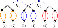
Figure 12: The treated example $\bar{C}_{6,\{1,2\}\{3,4\}\{5,6\},T}$.

This is better seen on an example: let us compute $\bar{C}_{6,\{1,2\}\{3,4\}\{5,6\},T}$, for $T$ as shown in Fig. 12. From Cor. 5.4, we have:

$$\bar{C}_{6,\{1,2\}\{3,4\}\{5,6\},T}(Y_{1},\ldots,Y_{6})=\mathcal{P}\circ\Bigl{(}\mathcal{D}^{\otimes}_{K_{2}}\,\mathcal{D}^{\otimes}_{K_{1}}\Bigr{)}\biggl{(}\tilde{C}_{2}(Y_{1},Y_{2})\otimes\tilde{C}_{2}(Y_{3},Y_{4})\otimes\tilde{C}_{2}(Y_{5},Y_{6})\biggr{)}.$$ (5.37)

We first let $\mathcal{D}^{\otimes}_{K_{1}}$ act on the argument, replacing $\tilde{C}_{2}$ by the expression (4.29), giving:

$$\mathcal{D}^{\otimes}_{K_{1}}\Bigl{(}\tilde{C}_{2}\otimes\tilde{C}_{2}\otimes\tilde{C}_{2}\Bigr{)}=\prod_{i=1}^{4}Y_{i}\frac{\partial}{\partial Y_{i}}\Biggl{(}\mathcal{D}^{\otimes}_{K_{1}}\biggl{(}\log(1-\hat{C}(Y_{1},Y_{2}))\otimes\log(1-\hat{C}(Y_{3},Y_{4}))\otimes\tilde{C}_{2}(Y_{5},Y_{6})\biggr{)}$$ (5.38)

$$\hskip 71.13188pt\prod_{i=1}^{4}Y_{i}\frac{\partial}{\partial Y_{i}}\Biggl{(}\hat{C}_{\{1,2\}\{3,4\}}(Y_{1},\ldots Y_{4})\biggl{(}\frac{1}{1-\hat{C}(Y_{1},Y_{2})}\otimes\frac{1}{1-\hat{C}(Y_{3},Y_{4})}\otimes\tilde{C}_{2}(Y_{5},Y_{6})\biggr{)}\Biggr{)}.$$

Letting now $\mathcal{D}^{\otimes}_{K_{2}}$ act on the result:

$$\mathcal{D}^{\otimes}_{K_{2}}\biggl{(}\mathcal{D}^{\otimes}_{K_{1}}\Bigl{(}\tilde{C}_{2}\otimes\tilde{C}_{2}\otimes\tilde{C}_{2}\Bigr{)}\biggr{)}=\prod_{i=1}^{6}Y_{i}\frac{\partial}{\partial Y_{i}}\Biggl{(}\hat{C}_{\{1,2\}\{3,4\}}(Y_{1},\ldots Y_{4})\hat{C}_{\{3,4\}\{5,6\}}(Y_{3},\ldots Y_{6})$$ (5.39)

$$\hskip 170.71652pt\biggl{(}\frac{1}{1-\hat{C}(Y_{1},Y_{2})}\otimes\frac{1}{(1-\hat{C}(Y_{3},Y_{4}))^{2}}\otimes\frac{1}{1-\hat{C}(Y_{5},Y_{6})}\biggr{)}\Biggr{)}.$$

Applying $\mathcal{P}$, we get the final result:

$$\bar{C}_{6,\{1,2\}\{3,4\}\{5,6\},T}(Y_{1},\ldots,Y_{6})=\prod_{i=1}^{6}Y_{i}\frac{\partial}{\partial Y_{i}}\Biggl{(}\frac{\hat{C}_{\{1,2\}\{3,4\}}(Y_{1},\ldots Y_{4})\hat{C}_{\{3,4\}\{5,6\}}(Y_{3},\ldots Y_{6})}{(1-\hat{C}(Y_{1},Y_{2}))(1-\hat{C}(Y_{3},Y_{4}))^{2}(1-\hat{C}(Y_{5},Y_{6}))}\Biggr{)}.$$ (5.40)

5.2 Simplifications

The relations of Borot et al. [2] reformulated in Thm. 2.7 are much simpler however, as some drastic simplifications occur. From Thm. 4.1 and Thm. 4.2, we see that the combinatorial proof of Thm. 2.6 equivalently formulated as Thm. 2.7 boils down to showing the following remarkable simplifications:

$$\sum_{T\in\mathcal{G}_{p}}\biggl{(}\prod_{i=1}^{p}X_{i}^{\mathrm{d}_{T}(i)-1}\frac{\mathrm{d}^{\mathrm{d}_{T}(i)-1}}{\mathrm{d}X_{i}^{\mathrm{d}_{T}(i)-1}}\biggr{)}\Biggl{\{}\prod_{i=1}^{p}{\frac{\mathrm{d}Y_{i}}{\mathrm{d}X_{i}}}\frac{1}{C(Y_{i})^{\mathrm{d}_{T}(i)}}\Biggl{(}\prod_{I\in\mathcal{I}(T)}H_{\lvert I\rvert}\bigl{(}Y_{I}\bigr{)}-\prod^{\prime}_{I\in\mathcal{I}(T)}\ C_{\lvert I\rvert}\bigl{(}Y_{I}\bigr{)}\Biggr{)}\Biggr{\}}=0,$$ (5.41)

where $\mathrm{d}_{T}(i)=\mathrm{deg}_{T}(i)$ and $Y_{I}=\{Y_{i}\}_{i\in I}$, $H_{\lvert I\rvert}$ is given by (4.15)

$$H_{\lvert I\rvert}=C_{\lvert I\rvert}+\sum_{\bar{\pi}\in\mathcal{P}^{*}(I)}\bar{H}_{\lvert I\rvert,\bar{\pi}},\qquad\bar{H}_{\lvert I\rvert,\bar{\pi}}=\sum_{T\in\mathcal{G}_{\bar{\pi}}}\bar{C}_{\lvert I\rvert,\bar{\pi},T},$$ (5.42)

where $\bar{C}_{\lvert I\rvert,\bar{\pi},T}$ is defined in (4.16), and $\prod^{\prime}$ means that any occurence of $C_{2}(Y_{1},Y_{2})$ should be replaced by

$$C_{2}(Y_{1},Y_{2})\quad\rightarrow\quad C_{2}(Y_{1},Y_{2})+\frac{Y_{1}Y_{2}}{(Y_{1}-Y_{2})^{2}}.$$ (5.43)

If $T$ has $I\in\mathcal{I}(T)$ with two elements (black vertices of valency two), the term $\prod_{I}H_{\lvert I\rvert}-\prod_{I}\ C_{\lvert I\rvert}$ is a sum of terms of the form $\prod_{I}O_{\lvert I\rvert}$, where $O_{\lvert I\rvert}$ is either $C_{\lvert I\rvert}$, or $\bar{C}_{\lvert I\rvert,\bar{\pi}}$ for some $\bar{\pi}\in\mathcal{P}^{*}(I)$, with the condition that not all $O_{\lvert I\rvert}$ are $C_{\lvert I\rvert}$. The corrections (5.43) must also be taken into account.

Because there are no relations among the $C_{p}(Y_{I})$, it should be true that the cancellations in (5.41) occur “order-by-order” in the $C_{k}(Y_{I})$, that is, all the terms involving for instance $C_{3}(Y_{1},Y_{2},Y_{3}),C_{2}(Y_{3},Y_{4}),C_{2}(Y_{4},Y_{5})$ should cancel among each other. Since there are no relations either among the $C_{p}$ and their derivatives for $p>1$, we expect the the cancellations to occur for each coefficient of an expression of the form $\frac{\partial}{\partial Y_{1}}C_{3}(Y_{1},Y_{2},Y_{3})\frac{\partial}{\partial Y_{1}}C_{2}(Y_{3},Y_{4})C_{2}(Y_{4},Y_{5})$. In particular, we expect that the terms that only involve $C_{1}$ should cancel among each other, implying an identity satisfied by $\tilde{C}_{p}$ for $p>2$:

$$\sum_{T\in\mathcal{G}_{p}}\biggl{(}\prod_{i=1}^{p}X_{i}^{\mathrm{d}_{T}(i)-1}\frac{\mathrm{d}^{\mathrm{d}_{T}(i)-1}}{\mathrm{d}X_{i}^{\mathrm{d}_{T}(i)-1}}\biggr{)}\Biggl{\{}\prod_{i=1}^{p}{\frac{\mathrm{d}Y_{i}}{\mathrm{d}X_{i}}}\frac{1}{C(Y_{i})^{\mathrm{d}_{T}(i)}}\Biggl{(}\prod_{I\in\mathcal{I}(T)}\tilde{C}_{\lvert I\rvert}\bigl{(}Y_{I}\bigr{)}$$ (5.44)

$$\hskip 199.16928pt-\prod_{I\in\mathcal{I}(T)}\prod_{i_{1},i_{2}\in\{1,\ldots,p\}}\delta_{I,\{i_{1},i_{2}\}}\frac{Y_{i_{1}}Y_{i_{2}}}{(Y_{i_{1}}-Y_{i_{2}})^{2}})\Biggr{)}\Biggr{\}}\ \raisebox{4.30554pt}{$\begin{subarray}{c}{?}\\ {=}\end{subarray}$}\ 0,$$ (5.45)

The last term is non-zero only if all the black vertices of the tree $T$ are of valency two. This identity would correspond to a recurrence satisfied by the $\tilde{C}_{p}$, as the term for the tree of $\mathcal{G}_{p}$ that has a single black vertex and all white vertices of valency one is just

$$\prod_{i=1}^{p}{\frac{\mathrm{d}Y_{i}}{\mathrm{d}X_{i}}}\frac{1}{C(Y_{i})}\tilde{C}_{p}(Y_{1},\ldots,Y_{p}),$$

and all the other terms involve $\tilde{C}_{k}$ for $k<p$. The relation can be extended to $\tilde{C}_{2}$ but it takes the different form (4.31):

$$\tilde{C}_{2}(Y_{1},Y_{2})-\frac{Y_{1}Y_{2}}{(Y_{1}-Y_{2})^{2}}=-\frac{Y_{1}Y_{2}}{(X_{1}-X_{2})^{2}}\frac{\mathrm{d}X_{1}}{\mathrm{d}Y_{1}}\frac{\mathrm{d}X_{2}}{\mathrm{d}Y_{2}},$$ (5.46)

instead of zero.

We then expect the contributions to (5.41) involving higher order free cumulants to derive from (5.44) by application of some differential operators on the identities satisfies by the $\tilde{C}_{k}$ for $k<p$. For instance, the other contributions to (5.41) for the tree of $\mathcal{G}_{p}$ that has a single black vertex and all white vertices of valency one are of the form

$$\prod_{i=1}^{p}{\frac{\mathrm{d}Y_{i}}{\mathrm{d}X_{i}}}\frac{1}{C(Y_{i})}\bar{C}_{\lvert I\rvert,\bar{\pi},T}=\prod_{i=1}^{p}{\frac{\mathrm{d}Y_{i}}{\mathrm{d}X_{i}}}\frac{1}{C(Y_{i})}\mathcal{P}\circ\Bigl{(}\prod_{K\in\mathcal{I(T)}}\mathcal{D}^{\otimes}_{K}\Bigr{)}\biggl{(}\,\bigotimes_{G\in K}\tilde{C}_{\lvert G\rvert}(Y_{G})\biggr{)},$$

for $I\subset\{1,\ldots,p\}$, $\bar{\pi}\in\mathcal{P}^{\star}(I)$, and $T\in\mathcal{G}_{\bar{\pi}}$, where we have applied Cor. 5.4.

Below, we detail this for the orders $p=3$ and $p=4$.

5.2.1 Third order

At third order $p=3$ for instance, there are two kinds of trees in $\mathcal{G}_{3}$, one with one black vertex and three with two black vertices, such that one white vertex has valency two and the two others valency one. The term in (5.41) for the first kind of tree has a weight $H_{3}-C_{3}$. From (4.33) (see also Fig. 9), the contribution to (5.41) from that tree is:

$$\prod_{i=1}^{3}{\frac{\mathrm{d}Y_{i}}{\mathrm{d}X_{i}}}\frac{1}{C(Y_{i})}\left(\tilde{C}_{3}+\bar{C}_{3,\{1\}\{2,3\}}+\bar{C}_{3,\{1,2\}\{3\}}+\bar{C}_{3,\{2\}\{1,3\}}\right)(Y_{1},Y_{2},Y_{3}),$$ (5.47)

whose expressions have been computed in Prop. 4.3. The term $\tilde{C}_{3}$ has only contributions of order 1, whereas the other three terms have contributions in $C_{2}$. For a tree with two black vertices and such that the white vertex labeled 1 has valency two, we get a weight

$$H_{2}(Y_{1},Y_{2})H_{2}(Y_{1},Y_{3})-\Bigl{(}C_{2}(Y_{1},Y_{2})+\frac{Y_{1}Y_{2}}{(Y_{1}-Y_{2})^{2}}\Bigr{)}\Bigl{(}C_{2}(Y_{1},Y_{3})+\frac{Y_{1}Y_{3}}{(Y_{1}-Y_{3})^{2}}\Bigr{)},$$

where $H_{2}=C_{2}+\tilde{C}_{2}$ (4.26), contributing to (5.41) as:

$$X_{1}\frac{\partial}{\partial X_{1}}\Biggl{(}\frac{C_{2}(Y_{1},Y_{2})\mathring{C}_{2}(Y_{1},Y_{3})+\mathring{C}_{2}(Y_{1},Y_{2}){C}_{2}(Y_{1},Y_{3})+\tilde{C}_{2}(Y_{1},Y_{2})\tilde{C}_{2}(Y_{1},Y_{3})-\frac{Y_{1}Y_{2}}{(Y_{1}-Y_{2})^{2}}\frac{Y_{1}Y_{3}}{(Y_{1}-Y_{3})^{2}}}{\prod_{i=1}^{3}{\frac{\mathrm{d}X_{i}}{\mathrm{d}Y_{i}}}C_{1}(Y_{1})^{2}C_{1}(Y_{2})C_{1}(Y_{3})}\Biggr{)},$$ (5.48)

where:

$$\mathring{C}_{2}(Y_{1},Y_{2})=\tilde{C}_{2}(Y_{1},Y_{2})-\frac{Y_{1}Y_{2}}{(Y_{1}-Y_{2})^{2}}=-\frac{Y_{1}Y_{2}}{(X_{1}-X_{2})^{2}}\frac{\mathrm{d}X_{1}}{\mathrm{d}Y_{1}}\frac{\mathrm{d}X_{2}}{\mathrm{d}Y_{2}}.$$ (5.49)

The contributions for the two other similar trees are obtained exchanging 1 and 2, and 1 and 3. From (5.41), the summation of these terms should vanish, and in fact the terms cancel “order by order”, that is the contributions involving $C_{2}$ cancel among each other. We simplify by the prefactor in (5.47).

Proposition 5.5.

The following simplifications occur at third order:

$$\tilde{C}_{3}(Y_{1},Y_{2},Y_{3})+\sum_{\begin{subarray}{c}{1\leftrightarrow 2}\\ {1\leftrightarrow 3}\end{subarray}}Y_{1}\frac{\partial}{\partial Y_{1}}\left({\frac{\mathrm{d}Y_{1}}{\mathrm{d}X_{1}}}\frac{\tilde{C}_{2}(Y_{1},Y_{2})\tilde{C}_{2}(Y_{1},Y_{3})-\frac{Y_{1}Y_{2}}{(Y_{1}-Y_{2})^{2}}\frac{Y_{1}Y_{3}}{(Y_{1}-Y_{3})^{2}}}{C_{1}(Y_{1})^{2}}\right)=0,$$ (5.50)

which involves only first order free cumulants and corresponds to (5.44), and

$$\bigl{(}\bar{C}_{3,\{1\}\{2,3\}}+\bar{C}_{3,\{1,2\}\{3\}}+\bar{C}_{3,\{1,3\}\{2\}}\bigr{)}\bigl{(}Y_{1},Y_{2},Y_{3}\bigr{)}$$ (5.51)

$$\hskip 85.35826pt+\sum_{\begin{subarray}{c}{1\leftrightarrow 2}\\ {1\leftrightarrow 3}\end{subarray}}Y_{1}\frac{\partial}{\partial Y_{1}}\left({\frac{\mathrm{d}Y_{1}}{\mathrm{d}X_{1}}}\frac{C_{2}(Y_{1},Y_{2})\mathring{C}_{2}(Y_{1},Y_{3})+\mathring{C}_{2}(Y_{1},Y_{2}){C}_{2}(Y_{1},Y_{3})}{C_{1}(Y_{1})^{2}}\right)=0,$$

which involves second order free cumulants and where $\mathring{C}_{2}$ is given in (5.49). This concludes the combinatorial proof of Thm. 2.7 for $p=3$.

Indeed, the second relation (5.51) is easily verified from (4.34) and is a particular case of Prop. 5.6. It is indeed true that the cancellations occur for each coefficient $C_{2}(Y_{a},Y_{b})$ and $\frac{\partial}{\partial Y_{a}}C_{2}(Y_{a},Y_{b})$ as can be seen from the proof of Prop. 5.6. The first relation (5.50) is much more involved, but we have verified it from (4.35) using Mathematica.

By replacing the expressions of $\tilde{C}_{2}$ and recognizing the results of some derivatives, we find an expression of $\tilde{C}_{3}$ which is well adapted for applying differential operators such as $\mathcal{D}$ or $\mathcal{P}\circ\Bigl{(}\prod_{K\in\mathcal{I(T)}}\mathcal{D}^{\otimes}_{K}\Bigr{)}$:

$$\tilde{C}_{3}(Y_{1},Y_{2},Y_{3})=\sum_{\begin{subarray}{c}{1\leftrightarrow 2}\\ {1\leftrightarrow 3}\end{subarray}}Y_{1}\frac{\partial}{\partial Y_{1}}Y_{2}\frac{\partial}{\partial Y_{2}}Y_{3}\frac{\partial}{\partial Y_{3}}\Biggl{(}\frac{Y_{3}}{Y_{1}-Y_{3}}\frac{Y_{2}}{Y_{1}-Y_{2}}\Biggl{[}\frac{1}{1-\hat{C}(Y_{1},Y_{2})}+\frac{1}{1-\hat{C}(Y_{1},Y_{3})}$$

$$\hskip 199.16928pt-\frac{C_{1}(Y_{1})^{2}\frac{\mathrm{d}X_{1}}{\mathrm{d}Y_{1}}}{(1-\hat{C}(Y_{1},Y_{2}))(1-\hat{C}(Y_{1},Y_{3}))}\Biggr{]}\Biggr{)}.$$ (5.52)

From this expression, we can indeed easily compute for instance $\bar{C}_{3,\{1,2,3\}\{4\}}(Y_{1},\ldots,Y_{4})=\mathcal{D}(\tilde{C}_{3}(Y_{1},Y_{2},Y_{3}),C_{1}(Y_{4}))$:

$$\bar{C}_{3,\{1,2,3\}\{4\}}(Y_{1},\ldots,Y_{4})=\sum_{\begin{subarray}{c}{1\leftrightarrow 2}\\ {1\leftrightarrow 3}\end{subarray}}Y_{1}\frac{\partial}{\partial Y_{1}}Y_{2}\frac{\partial}{\partial Y_{2}}Y_{3}\frac{\partial}{\partial Y_{3}}\Biggl{(}\frac{Y_{3}}{Y_{1}-Y_{3}}\frac{Y_{2}}{Y_{1}-Y_{2}}\Biggl{[}\frac{Y_{1}\frac{\partial}{\partial Y_{1}}C_{2}(Y_{1},Y_{4})-C_{2}(Y_{1},Y_{4})}{(1-\hat{C}(Y_{1},Y_{2}))(1-\hat{C}(Y_{1},Y_{3}))}$$

$$+\frac{\hat{C}_{\{1,2\}\{4\}}(Y_{1},Y_{2},Y_{4})}{(1-\hat{C}(Y_{1},Y_{2}))^{2}}\Biggl{(}1-\frac{C_{1}(Y_{1})^{2}\frac{\mathrm{d}X_{1}}{\mathrm{d}Y_{1}}}{1-\hat{C}(Y_{1},Y_{3})}\Biggr{)}+\frac{\hat{C}_{\{1,3\}\{4\}}(Y_{1},Y_{3},Y_{4})}{(1-\hat{C}(Y_{1},Y_{3}))^{2}}\Biggl{(}1-\frac{C_{1}(Y_{1})^{2}\frac{\mathrm{d}X_{1}}{\mathrm{d}Y_{1}}}{1-\hat{C}(Y_{1},Y_{2})}\Biggr{)}\Biggr{]}\Biggr{)}.$$ (5.53)

5.2.2 Contribution for $C_{p-1}$ at order $p$

It is easy to verify that at any order $p$, the terms involving the highest possible cumulants - the cumulants of order $p-1$ - cancel among themselves in (5.41), that is:

$$\prod_{i=1}^{p}{\frac{\mathrm{d}Y_{i}}{\mathrm{d}X_{i}}}\frac{1}{C_{1}(Y_{i})}\sum_{1\leq a<b\leq p}\bar{C}_{p,\{a,b\}}\bigl{(}Y_{1},\ldots,Y_{p}\bigr{)}+\sum_{a\neq b}X_{a}\frac{\partial}{\partial X_{a}}\left(\prod_{i=1}^{p}{\frac{\mathrm{d}Y_{i}}{\mathrm{d}X_{i}}}\frac{C_{p-1}(\{Y_{i}\}_{i\neq b})\mathring{C}_{2}(Y_{a},Y_{b})}{C_{1}(Y_{a})^{2}\prod_{i\neq a}C_{1}(Y_{i})}\right)=0,$$

which is in fact nothing more than (5.51). It follows from the following stronger fact.

Proposition 5.6.

For any $1\leq a<b\leq p$, it is true that:

$$\bar{C}_{p,\{a,b\}}\bigl{(}Y_{1},\ldots,Y_{p}\bigr{)}+Y_{a}\frac{\partial}{\partial Y_{a}}\left({\frac{\mathrm{d}Y_{a}}{\mathrm{d}X_{a}}}\frac{C_{p-1}(\{Y_{i}\}_{i\neq b})\mathring{C}_{2}(Y_{a},Y_{b})}{C_{1}(Y_{a})^{2}}\right)\ +\ a\leftrightarrow b=0.$$ (5.54)

where we we recall that $\bar{C}_{p,\{a,b\}}$ is $\bar{C}_{p,\bar{\pi}},$ for $\bar{\pi}$ the partition of $\{1,\ldots,p\}$ whose blocks all contain a single element, apart from the block $\{a,b\}$.

Proof.

The generating function $\bar{C}_{p,\{a,b\}}$ has been computed in (5.11) and (5.12) and found to be:

$$\bar{C}_{p,\{a,b\}}\bigl{(}Y_{1},\ldots,Y_{p}\bigr{)}=Y_{a}Y_{b}\frac{\partial}{\partial Y_{a}}\frac{\partial}{\partial Y_{b}}\left[\frac{Y_{b}C_{p-1}(\{Y_{i}\}_{i\neq b})-Y_{a}C_{p-1}(\{Y_{i}\}_{i\neq a})}{Y_{a}C_{1}(Y_{b})-Y_{b}C_{1}(Y_{a})}\right].$$ (5.55)

Noticing that

$$C_{1}(Y)-YC_{1}^{\prime}(Y)=C_{1}(Y)^{2}\frac{\mathrm{d}X}{\mathrm{d}Y},$$ (5.56)

we can carry out the derivatives, obtaining:

$$\bar{C}_{p,\{a,b\}}\bigl{(}Y_{1},\ldots,Y_{p}\bigr{)}=Y_{a}Y_{b}\frac{\partial}{\partial Y_{a}}\left[\frac{Y_{a}C_{1}(Y_{b})^{2}}{(Y_{a}C_{1}(Y_{b})-Y_{b}C_{1}(Y_{a}))^{2}}\frac{\mathrm{d}X_{b}}{\mathrm{d}Y_{b}}C_{p-1}(\{Y_{i}\}_{i\neq b})\right]\ +\ a\leftrightarrow b.$$ (5.57)

On the other hand,

$$Y_{a}\frac{\partial}{\partial Y_{a}}\Biggl{(}{\frac{\mathrm{d}Y_{a}}{\mathrm{d}X_{a}}}\frac{C_{p-1}(\{Y_{i}\}_{i\neq b})\mathring{C}_{2}(Y_{a},Y_{b})}{C_{1}(Y_{a})^{2}}\Biggr{)}=-Y_{a}\frac{\partial}{\partial Y_{a}}\Biggl{[}\frac{Y_{a}Y_{b}C_{1}(Y_{b})^{2}\frac{\mathrm{d}X_{b}}{\mathrm{d}Y_{b}}}{(Y_{a}C_{1}(Y_{b})-Y_{b}C_{1}(Y_{a}))^{2}}C_{p-1}(\{Y_{i}\}_{i\neq b})\Biggr{]},$$

which concludes the proof∎

While (5.55) was obtained in (5.11) as (5.10), that is, applying $\mathcal{D}$ to $\tilde{C}_{2}$ expressed in its logarithm form (4.29), the relation of Prop. 5.6 can be seen as applying $\mathcal{D}$ to $\tilde{C}_{2}$ in its formulation (4.31) but without the $X^{\prime}s$, that is:

$$\tilde{C}_{2}(Y_{1},Y_{2})=\frac{Y_{1}Y_{2}}{(Y_{1}-Y_{2})^{2}}\left(1-\frac{(C_{1}(Y_{1})-Y_{1}C_{1}^{\prime}(Y_{1}))(C_{1}(Y_{2})-Y_{2}C_{1}^{\prime}(Y_{2}))}{(1-\hat{C}(Y_{1},Y_{2}))^{2}}\right).$$ (5.58)

5.2.3 Fourth order

We now look more closely at (5.41) at order $p=4$. There are four kinds of trees in $\mathcal{G}_{4}$. The weight for the tree with one black vertex and four white vertices of valency one is $H_{4}-C_{4}$, where $H_{4}$ is given by (4.49). Recalling that $\mathring{C}_{2}$ is given by (5.49), the contribution to (5.41) is:

$$\prod_{i=1}^{4}{\frac{\mathrm{d}Y_{i}}{\mathrm{d}X_{i}}}\frac{1}{C(Y_{i})}\Bigl{(}\tilde{C}_{4}+\sum_{\mathrm{perm}}\bar{C}_{4,\{1\}\{2,3,4\}}+\sum_{\mathrm{perm}}\bar{C}_{4,\{1,2\}\{3,4\}}+\sum_{\mathrm{perm}}\bar{C}_{4,\{1\}\{2\}\{3,4\}}+\sum_{\mathrm{perm}}\bar{C}_{4,\{1\}\{2\}\{3,4\},T}\Bigr{)}.$$ (5.59)

The second kind of trees has one black vertex of valency 3, one black vertex $\{a,b\}$ of valency 2, one white vertex of valency two, and the other white vertices are of valency one. The weight for such trees is of the form $H_{3}H_{2}-C_{3}(C_{2}+Y_{a}Y_{b}/(Y_{a}-Y_{b})^{2})$. Carrying out the simplifications, the weight is of the form

$$C_{3}\mathring{C}_{2}+\bar{C}_{3,\{1\}\{2,3\}}C_{2}+\tilde{C}_{3}C_{2}+\bar{C}_{3,\{1\}\{2,3\}}\tilde{C}_{2}+\tilde{C}_{3}\tilde{C}_{2},$$

where all appropriate choices of labels and arguments must be taken into account. From left to right, the first term involves some $C_{3}$, the second some $C_{2}C_{2}$, the third and fourth some $C_{2}$, and the last only some $C_{1}$.

The third kind of trees has three black vertices $\{a,b\}$, $\{b,c\}$, $\{c,d\}$ of valency 2, two white vertices of valency two, and two white vertices of valency one. The weight for the black vertices of such trees is of the form $H_{2}H_{2}H_{2}-(C_{2}+Y_{a}Y_{b}/(Y_{a}-Y_{b})^{2})(C_{2}+Y_{b}Y_{c}/(Y_{b}-Y_{c})^{2})(C_{2}+Y_{c}Y_{d}/(Y_{c}-Y_{d})^{2})$. This can be recast as

$$\sum_{\mathrm{perm}}C_{2}C_{2}\mathring{C}_{2}+\sum_{\mathrm{perm}}C_{2}\Bigl{(}\tilde{C}_{2}\tilde{C}_{2}-\frac{Y_{a}Y_{b}}{(Y_{a}-Y_{b})^{2}}\frac{Y_{b}Y_{c}}{(Y_{b}-Y_{c})^{2}}\Bigr{)}+\tilde{C}_{2}\tilde{C}_{2}\tilde{C}_{2}-\frac{Y_{a}Y_{b}}{(Y_{a}-Y_{b})^{2}}\frac{Y_{b}Y_{c}}{(Y_{b}-Y_{c})^{2}}\frac{Y_{c}Y_{d}}{(Y_{c}-Y_{d})^{2}}.$$

The leftmost terms involve some $C_{2}C_{2}$, the second terms some $C_{2}$, and the two remaining terms only some $C_{1}$. The last kind of trees has three black vertices $\{a,b\}$, $\{a,c\}$, $\{a,d\}$ of valency two, but one white vertex of valency 3. The weights are just as above, but with adapted indices and arguments.

As mentioned above, the simplification (5.41) should occur “order-by-order”, that is here, we expect the terms corresponding to each item in the following list to cancel among each other (and coefficientwise for the various partial derivatives):

1. The terms involving $C_{3}$ (this we have already shown in Prop. 5.6),

2. The terms of the form $C_{2}(Y_{1},Y_{2}),C_{2}(Y_{1},Y_{3})$ with one repeated argument,

3. The terms of the form $C_{2}(Y_{1},Y_{2}),C_{2}(Y_{3},Y_{4})$,

4. The terms of the form $C_{2}(Y_{1},Y_{2})$,

5. The terms involving only the $C_{1}$.

In addition, we expect the simplifications to derive from (5.46) and (5.50), which are the simplifications for the terms involving only the $C_{1}$ for the lower orders $\tilde{C}_{2}$ and $\tilde{C}_{3}$.

We detail below the terms in $C_{2}C_{2}$. They are obtained from the following corrections:

$$\bar{C}_{4,\{1\}\{2\}\{3,4\},T},\ \ \bar{C}_{3,\{1\}\{2,3\}}C_{2},\ \textrm{ and }\ C_{2}C_{2}\mathring{C}_{2}.$$ (5.60)

In addition to $C_{2}C_{2}$, these only involve $\tilde{C}_{2}$ (and $C_{1}$), so we expect these simplifications to derive from applying differential operators such as $\mathcal{D}$ and $\mathcal{P}\circ\mathcal{D^{\otimes}}\mathcal{D^{\otimes}}$ to the identity (5.46). So to summarize, we expect the simplifications corresponding to the terms (5.60) to occur among each other:
$-\$among terms deriving from for instance $\tilde{C}_{2}(Y_{1},Y_{4})$,
$-\$among terms involving of the form $C_{2}(Y_{1},Y_{2}),C_{2}(Y_{1},Y_{3})$ with one repeated variable or of the form $C_{2}(Y_{1},Y_{2}),C_{2}(Y_{3},Y_{4})$ with disjoint variables, coefficientwise in the various partial derivatives.

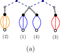
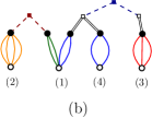
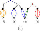
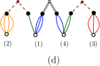
Figure 13: Diagrammatic representation of the contributions in $C_{2}(Y_{1},Y_{2})$ and $C_{2}(Y_{3},Y_{4})$ to the simplifications at order 4 that derive from the expression of $\tilde{C}_{2}(Y_{1},Y_{4})$. The red vertices and edges represent direct insertions of $C_{2}$, while the thick white edges and the blue vertices and edges represent corrections as in Fig. 9 and Fig. 11.

Focusing for instance on $\tilde{C}_{2}(Y_{1},Y_{4})$, $C_{2}(Y_{1},Y_{2})$ and $C_{2}(Y_{3},Y_{4})$, we get contributions from the diagrams in Fig. 13. We verify that these contributions to (5.41) simplify among each other, that is:

$$-Y_{1}Y_{4}\frac{\partial}{\partial Y_{1}}\frac{\partial}{\partial Y_{4}}\Bigl{(}\frac{Y_{1}Y_{4}}{(Y_{1}-Y_{4})^{2}}\frac{C_{2}(Y_{1},Y_{2})C_{2}(Y_{3},Y_{4})}{(1-\hat{C}(Y_{1},Y_{4}))^{2}}\Bigr{)}$$

$$+Y_{1}\frac{\partial}{\partial Y_{1}}\biggl{[}\frac{\mathrm{d}Y_{1}}{\mathrm{d}X_{1}}\frac{C_{2}(Y_{1},Y_{2})}{C(Y_{1})^{2}}Y_{1}Y_{4}\frac{\partial}{\partial Y_{1}}\frac{\partial}{\partial Y_{4}}\biggl{(}\frac{Y_{1}}{Y_{4}-Y_{1}}\frac{C_{2}(Y_{3},Y_{4})}{1-\hat{C}(Y_{1},Y_{2})}\biggr{)}\biggr{]}\ +\ \left\{\begin{array}[]{ll}1\leftrightarrow 4\\ 2\leftrightarrow 3\end{array}\right.$$ (5.63)

$$+Y_{1}Y_{4}\frac{\partial}{\partial Y_{1}}\frac{\partial}{\partial Y_{4}}\biggl{[}\frac{\mathrm{d}Y_{1}}{\mathrm{d}X_{1}}\frac{\mathrm{d}Y_{4}}{\mathrm{d}X_{4}}\frac{C_{2}(Y_{1},Y_{2})C_{2}(Y_{3},Y_{4})\mathring{C}_{2}(Y_{1},Y_{4})}{C(Y_{1})^{2}C(Y_{4})^{2}}\biggr{]}=0,$$ (5.64)

where line by line from the top, the terms come from $\bar{C}_{4,\{2\}\{3\}\{1,4\},T}$ (Fig. 13, (a)), $\bar{C}_{3,\{1,4\}\{3\}}$ (Fig. 13, (b)) and $\bar{C}_{3,\{1,4\}\{2\}}$ for the bracket (Fig. 13, (c)), and $C_{2}C_{2}\mathring{C}_{2}$ (Fig. 13, (d)).

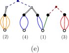
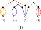
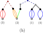
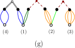
Figure 14: Remaining contributions in $C_{2},C_{2}$ to the simplifications at order 4 that derive from the expression of $\tilde{C}_{2}(Y_{1},Y_{4})$.

In the same way, the terms deriving from $\tilde{C}_{2}(Y_{1},Y_{4})$, and involving $C_{2}(Y_{1},Y_{2})$ and $C_{2}(Y_{1},Y_{3})$ cancel as:

$$Y_{1}Y_{4}\frac{\partial}{\partial Y_{1}}\frac{\partial}{\partial Y_{4}}\Bigl{(}\frac{Y_{4}^{2}}{(Y_{1}-Y_{4})^{2}}\frac{C_{2}(Y_{1},Y_{2})C_{2}(Y_{1},Y_{3})}{(1-\hat{C}(Y_{1},Y_{4}))^{2}}\Bigr{)}$$

$$+Y_{1}\frac{\partial}{\partial Y_{1}}\biggl{[}\frac{\mathrm{d}Y_{1}}{\mathrm{d}X_{1}}\frac{C_{2}(Y_{1},Y_{3})}{C(Y_{1})^{2}}Y_{1}Y_{4}\frac{\partial}{\partial Y_{1}}\frac{\partial}{\partial Y_{4}}\biggl{(}\frac{Y_{4}}{Y_{1}-Y_{4}}\frac{C_{2}(Y_{1},Y_{2})}{1-\hat{C}(Y_{1},Y_{4})}\biggr{)}\biggr{]}\quad+2\leftrightarrow 3$$ (5.65)

$$+X_{1}^{2}\frac{\partial^{2}}{\partial X_{1}^{2}}\Bigl{(}\frac{\mathrm{d}Y_{1}}{\mathrm{d}X_{1}}\frac{C_{2}(Y_{1},Y_{2})C_{2}(Y_{1},Y_{3})\mathring{C}_{2}(Y_{1},Y_{4})}{C_{1}(Y_{1})^{3}}\Bigr{)}=0,$$ (5.66)

where line by line from the top, the terms come from $\bar{C}_{4,\{2\}\{3\}\{1,4\},T}$ (Fig. 13, (a)), $\bar{C}_{3,\{1,4\}\{3\}}$ (Fig. 13, (b)) and $\bar{C}_{3,\{1,4\}\{2\}}$ for the bracket (Fig. 14, (e)), and $C_{2}C_{2}\mathring{C}_{2}$ (Fig. 14, (f)).

Finally, the remaining contributions in $C_{2}C_{2}$ involve other $C_{2}C_{2}$ for instance $C_{2}(Y_{1},Y_{2})C_{2}(Y_{2},Y_{3})$ and therefore also cancel among each other:

$$+Y_{2}\frac{\partial}{\partial Y_{2}}\biggl{[}\frac{\mathrm{d}Y_{2}}{\mathrm{d}X_{2}}\frac{C_{2}(Y_{2},Y_{3})}{C(Y_{2})^{2}}Y_{1}Y_{4}\frac{\partial}{\partial Y_{1}}\frac{\partial}{\partial Y_{4}}\biggl{(}\frac{Y_{4}}{Y_{1}-Y_{4}}\frac{C_{2}(Y_{1},Y_{2})}{1-\hat{C}(Y_{1},Y_{4})}\biggr{)}\biggr{]}$$ (5.67)

$$\hskip 85.35826ptY_{1}Y_{2}\frac{\partial}{\partial Y_{1}}\frac{\partial}{\partial Y_{2}}\biggl{[}\frac{\mathrm{d}Y_{1}}{\mathrm{d}X_{1}}\frac{\mathrm{d}Y_{2}}{\mathrm{d}X_{2}}\frac{C_{2}(Y_{1},Y_{2})C_{2}(Y_{2},Y_{3})\mathring{C}_{2}(Y_{2},Y_{4})}{C(Y_{1})^{2}C(Y_{2})^{2}}\biggr{]}=0,$$ (5.68)

where line by line from the top, the terms come from $\bar{C}_{3,\{1,4\}\{2\}}$ (Fig. 14, (g)), and $C_{2}C_{2}\mathring{C}_{2}$ (Fig. 14, (h)). There are terms of this kind involving $C_{2}(Y_{1},Y_{2})C_{2}(Y_{1},Y_{3})$ but they derive from $\tilde{C}_{2}(Y_{3},Y_{4})$ or $\tilde{C}_{2}(Y_{3},Y_{4})$ and cancel among each other.

In each case above, the simplifications presented are satisfied coefficientwise for the various partial derivatives $\frac{\partial}{\partial Y_{1}}C_{2}(Y_{1},Y_{2})C_{2}(Y_{1},Y_{3})$, $\frac{\partial}{\partial Y_{2}}C_{2}(Y_{1},Y_{2})C_{2}(Y_{1},Y_{3})$, etc.

This includes all the contributions in $C_{2},C_{2}$ by permutations of the indices. We formalize this in a proposition:

Proposition 5.7.

All the terms contributing to (5.41) that involve $C_{2},C_{2}$ cancel among each other.

We expect the same to occur among terms involving only one $C_{2}$, implying that (5.44) would be satisfied for $\tilde{C}_{4}$, and so on. This gives ground to the structure proposed at the beginning of Sec. 5.2, but a more efficient approach is needed to on one hand verify (5.44), and on the other, verify that it implies all the other simplifications in (5.41) via the application of differential operators such as $\mathcal{P}\circ\bigl{(}\prod_{K\in\mathcal{I(T)}}\mathcal{D}^{\otimes}_{K}\bigr{)}$. This is left for a future study.

References

- [1] G. Borot, S. Charbonnier, N. Do, E. Garcia-Failde, “Relating Ordinary and Fully Simple Maps via Monotone Hurwitz Numbers”, Electron. J. Comb. 26(3): 3 (2019), arXiv:1904.02267.
- [2] G. Borot, S. Charbonnier, E. Garcia-Failde, F. Leid, S. Shadrin, “Analytic theory of higher order free cumulants”, arXiv:2112.12184.
- [3] G. Borot, E. Garcia-Failde, “Simple Maps, Hurwitz Numbers, and Topological Recursion”, Commun. Math. Phys. 380, 581–654 (2020), arXiv:1710.07851.
- [4] W.G. Brown, “Enumeration of nonseparable planar maps”, Canad. J. Math. 15 (1963) 526–545.
- [5] W.G. Brown and W.T. Tutte, “On the enumeration of rooted nonseparable planar maps”, Canad. J. Math. 16 (1964), 572577.
- [6] B. Collins, “Moments and Cumulants of Polynomial random variables on unitary groups, the Itzykson-Zuber integral and free probability”, Int. Math. Res. Not. 2003(17), 953-982 (2003).
- [7] B. Collins, R. Gurau, L. Lionni, “The tensor Harish-Chandra–Itzykson–Zuber integral I: Weingarten calculus and a generalization of monotone Hurwitz numbers”, arXiv:2010.13661.
- [8] B. Collins and S. Matsumoto, “Weingarten calculus via orthogonality relations: new applications”, ALEA Lat. Am. J. Probab. Math. Stat. 2017(14), 631-656 (2017), arXiv:1701.04493.
- [9] B. Collins, J.A. Mingo, P. Sniady, R. Speicher, “Second Order Freeness and Fluctuations of Random Matrices, III. Higher order freeness and free cumulants”, Documenta Mathematica 12 (2007) 1-70, arXiv:math/0606431.
- [10] B. Collins, P. Śniady, “Integration with Respect to the Haar Measure on Unitary, Orthogonal and Symplectic Group,” Commun. Math. Phys. 264, 773-795 (2006), arXiv:math-ph/0402073.
- [11] A. Del Lungo, F. Del Ristoro, J-G. Penaud, “Left ternary trees and non-separable rooted planar maps”, Theor. Comput. Sci. 233(1-2): 201-215 (2000).
- [12] I.M. Gessel, “Lagrange inversion”, J. Combin. Theory A 144, 212–249 (2016).
- [13] I.P. Goulden, D.M. Jackson, Combinatorial Enumeration, Dover Books on Mathematics, Dover Publications (2004).
- [14] A. Hock, “On the x-y Symmetry of Correlators in Topological Recursion via Loop Insertion Operator”, arxiv: 2201.05357.
- [15] B. Jacquard and G. Schaeffer, “A bijective census of nonseparable planar maps”, J. Combin. Theory Ser. A, 83(1):1–20, (1998).
- [16] S. Matsumoto and J. Novak, “Jucys-Murphy elements and unitary matrix integrals,” Int. Math. Res. Not. IMRN. 2013(2), 362-397 (2013), arXiv:0905.1992.
- [17] J.A. Mingo, A. Nica, “Annular non-crossing permutations and partitions, and second-order asymptotics for random matrices”, Int. Math. Res. Not. 2004, no. 28, 1413–1460, arXiv:math/0303312.
- [18] J.A. Mingo, R. Speicher, “Second Order Freeness and Fluctuations of Random Matrices: I. Gaussian and Wishart matrices and Cyclic Fock spaces”, J. Funct. Anal. 235 (2006), no. 1, 226–270.
- [19] J.A. Mingo, P. Śniady, R. Speicher, “Second Order Freeness and Fluctuations of Random Matrices: II. Unitary Random Matrices”, Advances in Mathematics, Volume 209, Issue 1, 15 February 2007, Pages 212-240, arXiv:math/0405258.
- [20] A. Nica and R. Speicher, “Lectures on the combinatorics of free probability," volume 13. Cambridge University Press, (2006).
- [21] R. Speicher, “Free Probability Theory and Random Matrices”, In: Vershik A.M., Yakubovich Y. (eds) Asymptotic Combinatorics with Applications to Mathematical Physics. Lecture Notes in Mathematics, vol 1815. Springer, Berlin, Heidelberg (2003).
- [22] R. Speicher, “Multiplicative functions on the lattice of noncrossing partitions and free convolution”, Math. Ann., 298(4):611-628, 1994.
- [23] W.T. Tutte, “A census of planar maps”, Canad. J. Math. 15 (1963) 249–271.
- [24] D. Voiculescu, “Addition of certain non-commuting random variables”, J. Funct. Anal., 66: 323-346, 1986.
- [25] T.R.S. Walsh, “Hypermaps versus bipartite maps”, Journal of Combinatorial Theory (B) 18, 155-163 (1975).