Online Statistical Inference for Contextual Bandits via Stochastic Gradient Descent

Xi Chen111Stern School of Business, New York University, Email: xc13@stern.nyu.edu   Zehua Lai222Committee on Computational and Applied Mathematics, University of Chicago, Email: laizehua@uchicago.edu   He Li333Stern School of Business, New York University, Email: hli@stern.nyu.edu   Yichen Zhang444Krannert School of Management, Purdue University, Email: zhang@purdue.edu
Abstract

With the fast development of big data, it has been easier than before to learn the optimal decision rule by updating the decision rule recursively and making online decisions. We study the online statistical inference of model parameters in a contextual bandit framework of sequential decision-making. We propose a general framework for online and adaptive data collection environment that can update decision rules via weighted stochastic gradient descent. We allow different weighting schemes of the stochastic gradient and establish the asymptotic normality of the parameter estimator. Our proposed estimator significantly improves the asymptotic efficiency over the previous averaged SGD approach via inverse probability weights. We also conduct an optimality analysis on the weights in a linear regression setting. We provide a Bahadur representation of the proposed estimator and show that the remainder term in the Bahadur representation entails a slower convergence rate compared to classical SGD due to the adaptive data collection.

Keywords: online inference, stochastic gradient descent, contextual bandits, Bahadur representation, quantile regression

1 Introduction

Following the seminal work of Robbins (1952), the stochastic multi-armed bandit problem has been studied extensively in the literature, where an agent aims to make optimal decisions sequentially among multiple arms and only the selected arm reveals rewards consequently. As the agent’s choice is often influenced by additional covariates, also referred to as contexts, contextual bandit problems have gained renewed attention in the past decades (Woodroofe, 1979; Langford and Zhang, 2007, etc.). With the development of internet and data technology, contextual bandit algorithms play an important role in sequential decision-making applications, such as online advertisement (Li et al., 2010), precision medicine (Kim et al., 2011), e-commence (Qiang and Bayati, 2016; Chen et al., 2022), and public policy (Kasy and Sautmann, 2021). Such decisions are often referred to as recommendations, treatments, interventions, and public orders, while the rewards can be healthcare outcomes, welfare utility, revenue as well as any measure of satisfaction of decisions.

Most contextual bandit algorithms are built with the goal of learning the best action under different contexts. In sequential settings, it is often formulated as minimizing the expected cumulative regret that the practitioner would have received if she knows the optimal action. While the importance of this regret minimization is undisputed, reliable uncertainty quantification of the learned decision rule is evidently important in many featured applications. For example, in a personalized medicine application where the intervention decision is to choose t‘’he best medical treatment to optimize some health outcome, the risk for the selected treatment plays a critical and even sometimes life-threatening role in decision-making. Such examples call for the crucial need for a valid and reliable statistical inference procedure accompanying the decision-making process to provide guidance on policy interventions. Inferential studies help not only prompt risk alerts in recommendations, but also gain scientific knowledge of questions such as the effectiveness of medicines.

Particularly, consider a linear contextual bandit environment where the observed data at each decision point $t$ is a triplet $\zeta_{t}=(X_{t},A_{t},Y_{t})$ for all $t\geq 1$, consisting of covariate $X_{t}$, action $A_{t}$, and reward $Y_{t}=X_{t}^{\top}\theta_{A_{t}}^{*}+\epsilon_{t}$ where $\theta_{A_{t}}^{*}\in\mathbb{R}^{d}$ is unknown parameters of interest governed by a finite set of actions $\mathcal{A}$, and $\epsilon_{t}\in\mathbb{R}$ is the noise under certain modeling assumptions. For illustrative simplicity, we consider a binary action space $\mathcal{A}=\{0,1\}$ corresponding to a duplet of underlying model parameters $(\theta_{0}^{*},\theta_{1}^{*})\in\mathbb{R}^{d}\times\mathbb{R}^{d}$, and actions $A_{t}\in\mathcal{A}$ are selected according to a policy $A_{t}\sim\pi\left(X_{t},\mathcal{H}_{t-1}\right)$ where $\mathcal{H}_{t-1}$ denotes the trajectory of observations until time $t-1$. At the time $t$, a typical policy $\pi$ prefers the action with a higher mean reward $X_{t}^{\top}\theta_{a}^{*}$ for $a\in\mathcal{A}$, while reserving a small probability to explore a random action to avoid potential myopic short-sighted exploitation. For example, in the widely-used $\varepsilon$-greedy policy,

$\displaystyle\mathbb{P}\big{(}A_{t}=a\mid X_{t},\theta_{0,t-1},\theta_{1,t-1}\big{)}=(1-\varepsilon)\mathbbm{1}\big{\{}a=\mathop{\rm arg\max}_{a\in\mathcal{A}}X_{t}^{\top}\theta_{a,t-1}\big{\}}+\frac{\varepsilon}{2},$ (1)

This procedure heavily relies on a series of estimators $(\theta_{0,t-1},\theta_{1,t-1})$ on-the-fly, of the underlying model parameters. Despite that a return-oriented policy would undoubtedly favor the action with a higher reward, it is often as crucial to obtain the confidence of decisions, i.e., conducting statistical inference for $(\theta_{0}^{*},\theta_{1}^{*})$ in the prescribed applications. This model of statistical inference of model parameters in decision-making problems appears recently in literature (See e.g., Chen, Lu and Song, 2021a; Zhang, Janson and Murphy, 2021, and a brief survey in Section 1.1 below). A typical inferential task provides a confidence interval of the underlying parameters $(\theta_{0}^{*},\theta_{1}^{*})$ or significance levels when testing hypotheses of parameters, or its margin $\theta_{1}^{*}-\theta_{0}^{*}$.

Since the sequential decision-making problem relies on updating the estimator for every $t$ throughout the horizon, it is important to provide a computationally efficient fully-online algorithm for both estimation and inference purposes. The existing literature of sequential decision-making mostly focuses on the convergence rate and efficiency, while computational efficiency and storage applicability of the estimation algorithm is often optimistically neglected. As such, they often provide online decision-making procedures governed by an offline scheme of parameter estimation. At each iteration $t$, an “offline” $M$-estimator $(\theta_{0,t},\theta_{1,t})$ is often obtained using the sample path $\{(X_{1},y_{1}),\leavevmode\nobreak\ (X_{1},y_{2}),\dots,(X_{t},y_{t})\}$ up to time $t$. For example, when using the linear estimator, the computation cost accumulates in a non-scalable manner to at least $\mathcal{O}(T^{3})$ over the entire horizon $T$.

To facilitate computationally efficient online inference, we adopt the stochastic gradient descent (SGD) algorithms in conducting statistical inference in fully-online decision-making. SGD, dated back to Robbins and Monro (1951), has been widely used in large-scale stochastic optimization thanks to its computational and storage efficiency. Let $\theta_{0}$ denote an initial estimation, the SGD iteratively updates the parameter as follows,

$\displaystyle\theta_{t}=\theta_{t-1}-\eta_{t}\nabla\ell(\theta_{t-1};\zeta_{t}),$ (2)

where $\eta_{t}$ is a positive non-increasing sequence referred to as the step-size sequence and $\nabla\ell$ is the gradient for smooth individual loss function $\ell$. For the SGD update above, under the i.i.d. setting where $\zeta_{t}=(X_{t},Y_{t})$, the classical result by Polyak and Juditsky (1992) uses the average $\bar{\theta}_{t}^{{\tt{(SGD)}}}=t^{-1}\sum_{s=0}^{t-1}\theta_{s}$ as the final estimator to accelerate the estimation. They characterize the limiting distribution and statistical efficiency of the averaged SGD, i.e.,

$\displaystyle\sqrt{t}\big{(}\bar{\theta}^{{\tt{(SGD)}}}_{t}-\theta^{*}\big{)}\Longrightarrow\mathcal{N}\big{(}0,H^{{\tt{(SGD)}}-1}S^{{\tt{(SGD)}}}H^{{\tt{(SGD)}}-1}\big{)},$

given a series of predetermined learning rates $\eta_{t}=\eta_{0}t^{-\alpha}$ for $\eta_{0}>$ and $0.5<\alpha<1$. Here $H^{{\tt{(SGD)}}}$ and $S^{{\tt{(SGD)}}}$ are the Hessian and Gram matrix at $\theta=\theta^{*}$ for some population loss function under i.i.d. settings. For model well-specified settings, this asymptotic covariance matrix matches the inverse Fisher information matrix and thus the resulting averaged estimator $\bar{\theta}_{t}^{{\tt{(SGD)}}}$ is asymptotically efficient.

SGD fits well into the online decision-making scheme, as the underlying parameter $(\theta_{0}^{*},\theta_{1}^{*})$ is the solution to the following stochastic optimization under certain modeling assumptions,

$\displaystyle\theta_{a}^{*}\in\underset{\theta\in\mathbb{R}^{d}}{\operatorname{argmin}}\,\mathbb{E}\left[\ell\big{(}\theta;(X_{t},Y_{t})\big{)}\mid X_{t},A_{t}=a\right],\quad a\in\mathcal{A},$ (3)

where the function $\ell\in\mathbb{R}^{d}\to\mathbb{R}$ will be constructed accordingly. For example, in a linear contextual bandit $Y_{t}=X_{t}^{\top}\theta_{A_{t}}^{*}+\epsilon_{t}$ with i.i.d. covariates $X_{t}$ and mean-zero noise $\{\epsilon_{t}\}$, a natural choice of $\ell\big{(}\theta;(X_{t},Y_{t})\big{)}=\big{(}y_{t}-X_{t}^{\top}\theta\big{)}^{2}$ is the squared loss. As the outcome $Y_{t}$ at every time $t$ is adaptively collected upon the decision of action $A_{t}$, only one of the $\big{(}\theta_{0,t},\theta_{1,t}\big{)}$ is updated. To compensate missing updates, a generalized SGD updates

$\displaystyle\theta_{t}=\theta_{t-1}-\eta_{t}w_{t}\nabla\ell\big{(}\theta_{t-1};(X_{t},Y_{t})\big{)}.$ (4)

with a weighting parameter $w_{t}$ determined by the decision policy $\pi(X_{t},\mathcal{H}_{t-1})$. This procedure first appeared in Chen, Lu and Song (2021b) where they used the inverse probability weighting (IPW) for an $\varepsilon$-greedy policy (See (IPW) below for the explicit form of the weight). As a consequence, the weighted stochastic gradient $w_{t}\nabla\ell\big{(}\theta_{t-1};(X_{t},Y_{t})\big{)}$ is proved to be an unbiased estimator of a weighted population loss function where the weight is independent to the entire the historical information. While the unbiasedness property of stochastic gradient and its independence from the prior trajectory clear the technical difficulty of theoretical analysis of the asymptotic normality of the IPW-weighted ASGD estimator, IPW increases its asymptotic variance by a factor of $1/\varepsilon$. With such a factor, the proposed algorithm leads to a highly-volatile estimator in practice and entails an overly wide confidence interval while making inferential calls. Designing ameliorate decision-making algorithms to enhance the asymptotic efficiency of the estimator remains challenging yet important.

In this paper, we allow a general choice of the weighting parameter $w_{t}$ in (4), which admits the IPW weights as a special case, and derive the explicit formula for the asymptotic distribution of the generalized-weighting ASGD algorithm, thus provides us a way to compare different choices of $w_{t}$ and even optimize over $w_{t}$ for some simple models. Our proposed estimator greatly improves the asymptotic efficiency over IPW-ASGD and achieves comparable efficiency as if the practitioner picks one arm steadily. This estimator helps construct narrow yet reliable confidence intervals for the underlying parameter of interest. The analysis also reveals a recommendation of optimal choices of weights $w_{t}$ in certain policies. To overcome the technical challenge raised in dependent weighting parameters, we propose a new definition of the loss function, which is different from the loss function used in classical SGD literature (e.g., Chen et al., 2020) and adaptive SGD literature (Chen, Lu and Song, 2021b). We use two parameters $\theta$ and $\theta^{\prime}$ to separate the effect of weighting parameters in SGD and that of decision-making procedures in the local geometric landscape of the loss function.

As a separate interest, our framework allows non-smooth loss functions such as quantile loss. In contrast to linear regression, quantile regression provides estimates of a range of conditional quantiles of the reward $Y_{t}$. Since contextual bandit problems often appear in an interactive environment, the underlying reward model is more likely to differ across the distribution of the rewards and contexts or involves outliers. Linear regression methods estimate only the mean effects which is usually an incomplete summary of the effect of exposures for certain outcomes. For example, when recommending health care interventions, associations between health care and health outcomes can be highly different among individuals at high-, median-, and low-level utilization of health care. Quantile regression finds ubiquitous applications in many fields such as operations management of business inventory and risk management of financial assets (Rockafellar and Uryasev, 2002; Ban and Rudin, 2019). Therefore, it is worth exploring the use of quantile-based objective functions in sequential decision-making problems. In this paper, we establish a general framework that allows certain nonsmooth objective functions including quantile regression.

We emphasize the technical challenges and summarize the methodology contribution and theoretical advances in the following facets.

  • We study the online statistical inference of model parameters in a contextual bandit framework of sequential decision-making. We adopt the existing fully-online re-weighting algorithm for SGD but extend it in two directions: for a general choice of weights and handling non-smooth loss functions via stochastic subgradient. An important example is the quantile loss functions with applications in newsvendor problems and risk management. Moreover, this example provides robustness due to the fact that the objective function is globally Lipschitz. We establish the asymptotic normality result and characterize how the asymptotic covariance depends on the weight choice.

  • We show that SGD under $\varepsilon$-greedy policies with inverse probability weighting (IPW) in Chen, Lu and Song (2021b) suffers from an unbounded asymptotic variance when the exploration rate, $\varepsilon$ is close to 00, i.e., the relative efficiency of adaptive models versus non-adaptive models diverges to infinity. Our proposed algorithm features a general policy with a flexible specification of the weights to avoid such deficiency and obtain a bounded relative efficiency. We further provide some practical insights into the optimal weight specification.

  • Beyond the asymptotic normality of the proposed estimator, we further establish an analysis of the higher-order remainder term in its Bahadur representation. In classical i.i.d. SGD settings, the remainder term has the rate of $\mathcal{O}_{p}\big{(}t^{-\alpha+\frac{1}{2}}+t^{\alpha-1}\big{)}$. On the contrary, under the adaptive decision-making environment, the reminder term has a slower rate of $\mathcal{O}_{p}\big{(}t^{-\alpha+\frac{1}{2}}+t^{-\frac{\alpha}{4}}+t^{\alpha-1}\big{)}$. This slower rate can be considered as the effect of the discontinuous indicator function for the $\varepsilon$-greedy policy.

1.1 Related works

Online statistical inference for model parameters in SGD

The asymptotic distribution of averaged stochastic gradient descent (ASGD) is first given in Ruppert (1988) in Polyak and Juditsky (1992). Since then, there has been a rapid growth of interest recently in conducting statistical inference for model parameters in stochastic gradient algorithms. Chen et al. (2020) proposed two online estimators (plug-in and batch-means) in constructing estimators of limiting covariance matrix of ASGD, of which Zhu, Chen and Wu (2021) extended the batch-means to overlapped batches. Fang, Xu and Yang (2018) proposed a perturbation-based resampling procedure to conduct inference for ASGD. Su and Zhu (2018) proposed a tree-structured inference scheme to construct confidence intervals. Lee et al. (2022a, b) generalized the results in Polyak and Juditsky (1992) to a functional central limit theorem and proposed an online inference procedure called random-scaling for smooth objectives and quantile regression, respectively.

Statistical inference in online decision-making problems

Chen, Lu and Song (2021a) studied the asymptotic distribution of the parameters under a linear contextual bandit framework. Deshpande et al. (2018); Khamaru et al. (2021) considered adaptive linear regression where the vector contexts are correlated over time. Zhang, Janson and Murphy (2021, 2022) conducted statistical inference for M-estimators in contextual bandit and non-Markovian environments. Hao et al. (2019) used multiplier bootstrap to offer uncertainty quantification for exploration in the bandit settings. Chen, Lu and Song (2021b) conducted statistical inference under the contextual bandit settings via SGD. There also exists related statistical inference literature in reinforcement learning as a well-known online decision-making setting. Ramprasad et al. (2022) conducted statistical inference for TD (and GTD) learning. Shi et al. (2021) constructed the confidence interval for policy values in Markov decision processes. Shi et al. (2022) conducted statistical inference for confounded Markov decision processes. Chen, Song and Jordan (2022) developed the confidence interval for heterogeneous Markov decision processes.

1.2 Notations and organization of the paper

We first introduce some notations in our paper. For any pair of positive integers $m<n$, we use $[m:n]$ as a shorthand for the discrete set of $\{m,m+1,\ldots,n\}$. For any vector $\theta\in\mathbb{R}^{d}$, we use $\theta_{[m:n]}$ to denote the vector consisting of the $m$-th to $n$-th coordinates of $\theta$. Similarly, $\theta_{[m:n],t}$ is the corresponding subvector of $\theta_{t}$. For a set of random variables $X_{n}$ and a corresponding set of constants $a_{n}$, $X_{n}$ = $\mathcal{O}_{p}(a_{n})$ means that $X_{n}/a_{n}$ is stochastically bounded and $X_{n}=o_{p}(a_{n})$ means that $X_{n}/a_{n}$ converges to zero in probability as $n$ goes to infinity. We denote $\overset{p}{\rightarrow}$, and $\overset{d}{\rightarrow}$ as convergence in probability and convergence in distribution, respectively.

For convenience, let $\|\cdot\|$ denote the standard Euclidean norm for vectors and the spectral norm for matrices. We use the standard Loewner order notation $\Sigma\succeq 0$ if a matrix $\Sigma$ is positive semi-definite. Denote $I_{d}$ as the identity matrix in $\mathbb{R}^{d\times d}$. For any square matrix $\Sigma$, $\lambda_{\min}(\Sigma)$ and $\lambda_{\max}(\Sigma)$ represent the smallest and the largest eigenvalues, respectively. We also introduce $\mathbbm{1}(\cdot)$ for the indicator function, and $\lesssim$ is used for inequalities with omitted constants.

The remainder of the paper is organized as follows. In Section 2, we consider the environment where we collect data adaptively. We describe the weighted version SGD under this setting and give two illustrative examples of the classical regression problems. In Section 4, we first introduce the technical assumptions before we present the asymptotic distribution for general weighted SGD under this adaptive data collection scheme, along with a comparison on the statistical efficiency to the previous result proposed in Chen, Lu and Song (2021b). We further justify our assumptions under the two illustrative regression examples and show the asymptotic normality for these two cases. Section 4.2 gives the finite-sample rate for our SGD update under adaptive environment. We compare our result with the classical SGD rate, where the slower rate is due to the adaptively collected data. Simulation studies and real data analyses in Section 5 lend numerical support to the theoretical claims in this paper, which also provides hands-on guidelines to practitioners.

2 Problem Setup

We consider a contextual bandit environment where the observed data at each decision point $t$ is a triplet $\zeta_{t}=(X_{t},A_{t},Y_{t})$ for all $t\geq 1$, consisting of covariate $X_{t}$, action $A_{t}$, and reward $Y_{t}$. In this paper, we consider a finite action space, i.e., $A_{t}\in\mathcal{A}$ and $|\mathcal{A}|<\infty$. We assume a stochastic contextual bandit environment in which $\left\{X_{t},Y_{t}(a):a\in\mathcal{A}\right\}\stackrel{{\scriptstyle i.i.d}}{{\sim}}\mathcal{P}\in\mathbf{P}$ for all $t\geq 1$. The contextual bandit environment distribution $\mathcal{P}$ is in a space of possible environment distributions $\mathbf{P}$. Here $Y_{t}(a)$ corresponds to the (heuristic) reward $Y_{t}$ given a fixed action $a$ regardless of the realized action $A_{t}$. Note that $Y_{t}(a)$ is observed for $a=A_{t}$ only, but not observed for any other $a\in\mathcal{A},a\neq A_{t}$.

We define the trajectory until time $t$ as $\mathcal{H}_{t}:=\left\{X_{s},A_{s},Y_{s}\right\}_{s=1}^{t}$ for $t\geq 1$ and $\mathcal{H}_{0}:=\emptyset$. Actions $A_{t}\in\mathcal{A}$ are selected according to some policy $A_{t}\sim\pi\left(X_{t},\mathcal{H}_{t-1}\right)$, which defines action distribution. Even though the covariate reward tuples are i.i.d., the observed data $\left\{X_{t},A_{t},Y_{t}\right\}_{t\geq 1}$ are not i.i.d., since the actions are selected using policies $\pi\left(X_{t},\mathcal{H}_{t-1}\right)$ which is a function of past data, $\mathcal{H}_{t-1}$. Non-independence of observations is a key property of adaptively collected data.

We are interested in constructing confidence regions for some unknown $\theta^{*}\in\mathbb{R}^{d}$. Under the finite action space where $|\mathcal{A}|<\infty$, we can use $\theta^{*}$ as the concatenated vector of $\theta_{a}^{*}$ for all $a\in\mathcal{A}$, where we assume that $\theta^{*}_{a}$ is a conditionally maximizing value of some loss function $\ell(\theta;\zeta)$ for $\mathcal{P}\in\mathbf{P}$,

$\displaystyle\theta_{a}^{*}(\mathcal{P})\in\underset{\theta\in\mathbb{R}^{d}}{\operatorname{argmin}}\,\mathbb{E}_{\mathcal{P}_{Y\mid X}}\left[\ell\left(\theta;\zeta\right)\mid X,A=a\right].$ (5)

Note that (5) represents an implicit modeling assumption that such an underlying $\theta_{a}^{*}$ does not depend on $X$ for a given loss $\ell(\theta;\zeta)$. This assumption is generally satisfied in many statistical applications. For example, in a classical regression setting, a natural choice for $\ell(\theta;\zeta)$ is as follows,

$\displaystyle\ell(\theta;\zeta_{t})=\rho\left(Y_{t}-X_{t}^{\top}\theta_{A_{t}}\right),\;\;$ (6)

where $\theta\in\mathbb{R}^{d}$ is the concatenated vector of $\theta_{A_{t}}\in\mathbb{R}^{p}$ for all possible choices of $A_{t}\in\mathcal{A}$ and $d=p|\mathcal{A}|$. Here $\rho(\cdot)$ is some convex loss function. Note that $\ell$ can be non-smooth as long as $\nabla\ell$ exists almost surely. We illustrate several examples of popular statistical models, and we will refer to these examples throughout the paper.

Example 2.1 (Linear Regression).

Consider a two-arm linear contextual bandit problem where

$\displaystyle\mathbb{E}[Y_{t}\mid A_{t},X_{t}]=X_{t}^{\top}\theta^{*}_{A_{t}}=(1-A_{t})\big{(}X_{t}^{\top}\theta^{*}_{[1:p]}\big{)}+A_{t}\big{(}X_{t}^{\top}\theta^{*}_{[p+1:2p]}\big{)},$

where $\theta^{*}\in\mathbb{R}^{d}$ is the concatenated vector of $\theta^{*}_{[1:p]}$ and $\theta^{*}_{[p+1:2p]}$ and $\theta^{*}_{[1:p]}\neq\theta^{*}_{[p+1:2p]}$, $\left\{X_{t},Y_{t}(a):a\in\mathcal{A}\right\}$ $\stackrel{{\scriptstyle i.i.d}}{{\sim}}\mathcal{P}\in\mathbf{P}$ for all $t\geq 1$, and $\mathcal{A}=\{0,1\}$. The true reward $Y_{t}$ is generated by $\mathbb{E}[Y_{t}\mid A_{t},X_{t}]+\mathcal{E}_{t}$ where $\{\mathcal{E}_{t}\}$ are i.i.d. random error with mean zero and variance $\sigma^{2}$. Under the linear regression model, our loss function $\ell$ is defined as

$\displaystyle\ell(\theta;\zeta_{t})=\frac{1}{2}(1-A_{t})\left(Y_{t}-X_{t}^{\top}\theta_{[1:p]}\right)^{2}+\frac{1}{2}A_{t}\left(Y_{t}-X_{t}^{\top}\theta_{[p+1:2p]}\right)^{2}.$
Example 2.2 (Logistic Regression).

Consider a two-arm contextual bandit problem under the logistic model with binary rewards where $A_{t}\in\mathcal{A}=\{0,1\}$, $Y_{t}\in\{-1,1\}$, and

$\displaystyle\mathcal{P}(Y_{t}\mid A_{t},X_{t})=\left(1+\exp\left(-(1-A_{t})Y_{t}X_{t}^{\top}\theta^{*}_{[1:p]}+-A_{t}Y_{t}X_{t}^{\top}\theta^{*}_{[p+1:2p]}\right)\right)^{-1}.$

We consider the entropy loss

$\displaystyle\ell(\theta;\zeta_{t})=(1-A_{t})\log\left(1+\exp\left(-Y_{t}X_{t}^{\top}\theta_{[1:p]}\right)\right)+A_{t}\log\left(1+\exp\left(-Y_{t}X_{t}^{\top}\theta_{[p:2p]}\right)\right).$
Example 2.3 (Quantile Regression).

Consider a two-arm linear contextual bandit problem where

$\displaystyle Y_{t}=(1-A_{t})X_{t}^{\top}\theta^{*}_{[1:p]}+A_{t}X_{t}^{\top}\theta^{*}_{[p+1:2p]}+\mathcal{E}_{t},$

and $\{\mathcal{E}_{t}\}$ are i.i.d. random error such that, $\mathbb{P}(\mathcal{E}_{t}\leq 0)=\tau$ for some given quantile level $\tau\in(0,1)$. Consider a quantile loss such that

$\displaystyle\ell(\theta;\zeta_{t})=(1-A_{t})\rho_{\tau}\left(Y_{t}-X_{t}^{\top}\theta_{[1:p]}\right)+A_{t}\rho_{\tau}\left(Y_{t}-X_{t}^{\top}\theta_{[p+1:2p]}\right),$

where $\rho_{\tau}(u)=u(\tau-\mathbbm{1}(u<0))$.

3 SGD with weighted stochastic gradients

Under the adaptive data collection scheme, we now consider a generalized version of the classical SGD (2) with weights $w_{t}$ depends only on the triplet $(A_{t},X_{t},\theta_{t-1})$, as follows,

$\displaystyle\theta_{t}=\theta_{t-1}-\eta_{t}w_{t}\nabla\ell(\theta_{t-1};\zeta_{t}).$ (7)

We consider the following three popular choices of weight $w_{t}$ as examples throughout the paper.

  1. (IPW)

    Inverse probability weighting: $w_{t}(A_{t},X_{t},\theta_{t-1})=\dfrac{1}{2\,\mathbb{P}(A_{t}\mid X_{t},\theta_{t-1})}$.

  2. (sqrt-IPW)

    Square-root importance weights: $w_{t}(A_{t},X_{t},\theta_{t-1})=\sqrt{\dfrac{1}{2\,\mathbb{P}(A_{t}\mid X_{t},\theta_{t-1})}}$.

  3. (vanilla)

    No weights applied to the SGD updates. $w_{t}(A_{t},X_{t},\theta_{t-1})=1$.

These weighting schemes are well-rooted in literature, such as (IPW)  by Chen, Lu and Song (2021b) that corrects the action distribution to some deterministic stable policy, and (sqrt-IPW)  in Hammersley (2013) and Zhang, Janson and Murphy (2021). The proposed method is not limited to the analysis of these three weights but is applied to general weight specifications. Before we present our main result, we revisit the three aforementioned motivating examples and illustrate the weighted SGD algorithm for the three models.

Example 2.1 (Continued).

Under the linear regression model, the weighted SGD (7) writes as

$\displaystyle\theta_{[1:p],t}$ $\displaystyle=\theta_{[1:p],t-1}-\eta_{t}w_{t}X_{t}\left(X_{t}^{\top}\theta_{[1:p],t-1}-Y_{t}\right),\;\;A_{t}=0;$
$\displaystyle\theta_{[p+1:2p],t}$ $\displaystyle=\theta_{[p+1:2p],t-1}-\eta_{t}w_{t}X_{t}\left(X_{t}^{\top}\theta_{[p+1:2p],t-1}-Y_{t}\right),\;\;A_{t}=1.$
Example 2.2 (Continued).

Under a logistic regression model, the weighted SGD (7) writes as

$\displaystyle\theta_{[1:p],t}$ $\displaystyle=\theta_{[1:p],t-1}+\eta_{t}w_{t}\left(1+\exp\big{(}Y_{t}X_{t}^{\top}\theta_{[1:p],t-1}\big{)}\right)^{-1}Y_{t}X_{t},\;\;A_{t}=0;$
$\displaystyle\theta_{[p+1:2p],t}$ $\displaystyle=\theta_{[p+1:2p],t-1}+\eta_{t}w_{t}\left(1+\exp\big{(}Y_{t}X_{t}^{\top}\theta_{[p+1:2p],t-1}\big{)}\right)^{-1}Y_{t}X_{t},\;\;A_{t}=1.$
Example 2.3 (Continued).

Under the quantile regression model, the weighted SGD (7) writes as

$\displaystyle\theta_{[1:p],t}$ $\displaystyle=\theta_{[1:p],t-1}+\eta_{t}w_{t}\left(\tau-\mathbbm{1}(Y_{t}-X_{t}^{\top}\theta_{[1:p],t-1}<0)\right)X_{t},\;\;A_{t}=0;$
$\displaystyle\theta_{[p+1:2p],t}$ $\displaystyle=\theta_{[p+1:2p],t-1}+\eta_{t}w_{t}\left(\tau-\mathbbm{1}(Y_{t}-X_{t}^{\top}\theta_{[p+1:2p],t-1}<0)\right)X_{t},\;\;A_{t}=1.$

Given our path of $\{\theta_{t}\}_{t\geq 1}$, we assume the policy $\pi\left(X_{t},\mathcal{H}_{t-1}\right)$ depend on the history $\mathcal{H}_{t-1}$ only through $\theta_{t-1}$, our estimator from the latest step, i.e., $A_{t}\sim\pi\left(X_{t},\theta_{t-1}\right)$. We consider a common policy, $\varepsilon$-greedy, to address the exploration-and-exploitation dilemma, where the probability of action $A_{t}$ is defined as,

$\displaystyle\mathbb{P}(A_{t}=0\mid X_{t},\theta_{t-1})=(1-\varepsilon)\mathbbm{1}\left\{X_{t}^{\top}\theta_{[1:p],t-1}>X_{t}^{\top}\theta_{[p+1:2p],t-1}\right\}+\frac{\varepsilon}{2},$ (8)

for some constant $\varepsilon\in(0,1)$. In practice, the $\varepsilon$ is often set as some small constant close to zero. Note that this setting can be relaxed to a deterministic sequence $\{\varepsilon_{t}\}$ which converges to some constant $\varepsilon_{\infty}\in(0,1)$. Note that this may be relaxed to $A_{t}\sim\pi\left(X_{t},\Phi_{t-1}\right)$ for some other statistic $\Phi_{t-1}$ relies on the history $\theta_{0},\theta_{1},\cdots,\theta_{t-1}$, for example, the running average of the $\{\theta_{s}\}_{s=0}^{t-1}$.

We now use the linear regression model in Example 2.1 with random design as a special case of our main result that will be presented in Theorem 4.2 below. We specify $w_{t}$ as a function of $\mathbb{P}(A_{t}\mid X_{t},\theta_{t-1})$, i.e., $w_{t}(A_{t},X_{t},\theta_{t-1})=\varphi(\mathbb{P}(A_{t}\mid X_{t},\theta_{t-1}))$. The following Theorem 3.1 provides a new way to further determine the optimal weighting scheme to minimize the asymptotic variance of the average SGD estimator.

Theorem 3.1.

In the linear regression setting in Example 2.1, assume that $X_{t}\sim\mathcal{N}(\mu,I_{p})$, and $\varphi(\cdot):(0,1)\mapsto\mathbb{R}^{+}$ is continuous. The averaged SGD estimator $\bar{\theta}_{t}$ converges to $\theta^{*}$ almost surely as $t\rightarrow\infty$ and

$\displaystyle\sqrt{t}(\bar{\theta}_{t}-\theta^{*})\overset{d}{\rightarrow}\mathcal{N}(0,H^{-1}SH^{-1}),\quad\text{where }$ $\displaystyle S$ $\displaystyle=\begin{bmatrix}S_{1}&0\\ 0&S_{2}\end{bmatrix},\leavevmode\nobreak\ H=\begin{bmatrix}H_{1}&0\\ 0&H_{2}\end{bmatrix},$
$\displaystyle S_{1}$ $\displaystyle=\sigma^{2}\left((1-\frac{\varepsilon}{2})\varphi^{2}(1-\frac{\varepsilon}{2})G_{1}^{*}+\frac{\varepsilon}{2}\varphi^{2}(\frac{\varepsilon}{2})G_{2}^{*}\right),\;\;$ $\displaystyle S_{2}$ $\displaystyle=\sigma^{2}\left(\frac{\varepsilon}{2}\varphi^{2}(\frac{\varepsilon}{2})G_{1}^{*}+(1-\frac{\varepsilon}{2})\varphi^{2}(1-\frac{\varepsilon}{2})G_{2}^{*}\right),$
$\displaystyle H_{1}$ $\displaystyle=(1-\frac{\varepsilon}{2})\varphi(1-\frac{\varepsilon}{2})G_{1}^{*}+\frac{\varepsilon}{2}\varphi(\frac{\varepsilon}{2})G_{2}^{*},\;\;$ $\displaystyle H_{2}$ $\displaystyle=\frac{\varepsilon}{2}\varphi(\frac{\varepsilon}{2})G_{1}^{*}+(1-\frac{\varepsilon}{2})\varphi(1-\frac{\varepsilon}{2})G_{2}^{*},$
$\displaystyle G_{1}^{*}$ $\displaystyle=\Phi\left(a^{*}\right)I_{p}+\frac{1}{\sqrt{2\pi}}a^{*}e^{\frac{a^{*2}}{2}}\nu^{*}\nu^{*\top},$ $\displaystyle G_{2}^{*}$ $\displaystyle=\left(1-\Phi\left(a^{*}\right)\right)I_{p}-\frac{1}{\sqrt{2\pi}}a^{*}e^{\frac{a^{*2}}{2}}\nu^{*}\nu^{*\top},$

and $\nu^{*}=(\theta^{*}_{[1:p]}-\theta^{*}_{[p+1:2p]})/\|\theta^{*}_{[1:p]}-\theta^{*}_{[p+1:2p]}\|$, $a^{*}=\frac{\mu^{\top}\nu^{*}}{\sqrt{1+(\mu^{\top}\nu^{*})^{2}}}$, and $\Phi$ is the cumulative distribution function of standard normal distribution.

Theorem 3.1 can be considered as a special case of our main result which will be presented in 4. The proof of Theorem 3.1 is provided in Appendix A. Here the definition of $\nu^{*}$ and consequently the existence of the asymptotic covariance matrix are assured by the implicit non-degenerate model assumption such that $\theta^{*}_{[1:p]}\neq\theta^{*}_{[p+1:2p]}$.

In light of Theorem 3.1, we are ready to conduct a comparison among the three popular weighting schemes. Here we specify $\varphi_{\gamma}(\varepsilon)=\varepsilon^{\gamma}$ as a class of power functions parameterized by $\gamma$. This class of weights covers the following three popular weighting schemes: (IPW) as $\gamma=-1$, (sqrt-IPW) as $\gamma=-1/2$, and (vanilla) as $\gamma=0$, up to some constants. Since $H_{1},H_{2},G_{1},G_{2}$ all have the form $\tilde{b}I+\tilde{c}\nu^{*}\nu^{*\top}$ for some constants $\tilde{b}$ and $\tilde{c}$, they can be simultaneously diagonalized. With details due in Appendix, we can explicitly compute the eigenvalues and eigenvectors of the asymptotic covariance matrix $H^{-1}SH^{-1}$. With detailed derivation relegated to Appendix B, we can show that when varying $\gamma$, the eigenvectors stay fixed and each eigenvalue changes in the following form with some $b\in(0,1)$,

$\displaystyle g(\gamma)=\frac{(1-\varepsilon/2)^{1+2\gamma}b+(\varepsilon/2)^{1+2\gamma}(1-b)}{\big{(}(1-\varepsilon/2)^{1+\gamma}b+(\varepsilon/2)^{1+\gamma}(1-b)\big{)}^{2}}.$ (9)

In practice, for the $\varepsilon$-greedy policy, the parameter $\varepsilon$ is usually taken as some small constant. When $\varepsilon$ gets close to 00, it can be inferred from (9) that $\gamma\geq-1/2$ leads to a finite covariance matrix even when $\varepsilon$ goes to zero, while $\gamma<-1/2$ leads to an infinite covariance matrix. This includes (vanilla)  and (sqrt-IPW)  but excludes (IPW). Furthermore, the minimum of (9) is obtained at $\gamma=0$ for all $b\in(0,1)$. Therefore, under the settings in Theorem 3.1, (vanilla)  has an asymptotic covariance matrix that is dominated by any other asymptotic covariance matrix obtained from a power-law weighted scheme, $\varphi(\varepsilon)=\varepsilon^{\gamma}$. The following Corollary 3.2 concludes the above discussion and further extends to general weighting schemes $w$.

Corollary 3.2 (Optimal weights in linear regression).

Under Assumption 1 to Assumption 5, the (vanilla)SGD has the optimal asymptotic covariance matrix in the linear regression setting, i.e., $\Sigma_{\mathrm{vnl}}\preceq\tilde{\Sigma}$, where $\Sigma_{\mathrm{vnl}}$ is the asymptotic covariance matrix of vanilla SGD and $\tilde{\Sigma}$ is the asymptotic covariance matrix under any other weighting function $\varphi$ where $w_{t}(A_{t},X_{t},\theta_{t-1})=\varphi(\mathbb{P}(A_{t}\mid X_{t},\theta_{t-1}))$.

4 Asymptotic normality under general models

We provide the main theoretical results in this section with detailed proof relegated to Appendix. To facilitate the analysis of the asymptotic behavior of SGD update (7) in a general model, we define the function $\mathcal{L}_{\theta^{\prime}}(\theta)$ as follows,

$\displaystyle\mathcal{L}_{\theta^{\prime}}(\theta)=\mathbb{E}_{\mathcal{P}}\left[\mathbb{E}_{\pi(X,\theta^{\prime})}\left(w(\theta^{\prime};X,A)\ell(\theta;X,A,Y)\mid X\right)\right],$ (10)

where $A\sim\pi(X,\theta^{\prime})$, $\theta^{\prime},\theta\in\mathbb{R}^{d}$, and gradient weight $w$ depending on $\theta^{\prime}$, action $A$ and covariate $X$. Note that the objective $\mathcal{L}_{\theta^{\prime}}(\theta)$ is a function of $\theta$ with a parameter $\theta^{\prime}$ that corresponds to the current estimate being used to select the action. Typically we use $\theta^{\prime}=\theta_{t-1}$ at iteration $t$. Below we will always use the expression $\nabla\mathcal{L}_{\theta^{\prime}}(\theta)$ to represent the partial gradient of $\mathcal{L}_{\theta^{\prime}}(\theta)$ with respect to the variable $\theta$, i.e.,

$\displaystyle\nabla\mathcal{L}_{\theta^{\prime}}(\theta)=\frac{\partial}{\partial\theta}\mathcal{L}_{\theta^{\prime}}(\theta)\in\mathbb{R}^{d},\;\;\nabla^{2}\mathcal{L}_{\theta^{\prime}}(\theta)=\frac{\partial^{2}}{\partial\theta^{2}}\mathcal{L}_{\theta^{\prime}}(\theta)\in\mathbb{R}^{d\times d}.$

We note that for quantile regression in Example 2.3, even though the individual objective $\ell(\theta;X,Y)$ is nonsmooth, the population objective $\mathcal{L}_{\theta^{\prime}}(\theta)$ is second-order differentiable with some smoothness conditions on the error distribution. Finally, we denote $\xi_{\theta^{\prime}}(\theta;\zeta)$ as the difference between the stochastic gradient and population gradient of the loss defined in (10), i.e.,

$\displaystyle\xi_{\theta^{\prime}}(\theta;\zeta)=w(\theta^{\prime};X,A)\nabla\ell(\theta;\zeta)-\nabla\mathcal{L}_{\theta^{\prime}}(\theta),$ (11)

By definition, we can easily verify that $w(\theta^{\prime};X,A)\nabla\ell(\theta;\zeta)$ is an unbiased estimator of $\nabla\mathcal{L}_{\theta^{\prime}}(\theta)$, $\mathbb{E}[\xi_{\theta^{\prime}}(\theta;\zeta)]=0$.

In the previous work of Chen, Lu and Song (2021b), the loss function is defined with respect to some pre-determined stable policy $\pi_{\mathrm{stable}}$, i.e.,

$\displaystyle\tilde{\mathcal{L}}(\theta)=\mathbb{E}_{\mathcal{P}}\left[\mathbb{E}_{\pi_{\mathrm{stable}}}\left(\ell(\theta;X,A,Y)\mid X\right)\right],$ (12)

where $A\sim\pi_{\mathrm{stable}}$ and $\pi_{\mathrm{stable}}$ is a Bernoulli($1/|\mathcal{A}|$), uniformly distributed on the action space $\mathcal{A}$. To match the SGD update with the loss function $\tilde{\mathcal{L}}(\cdot)$, they choose the (IPW)-weighted SGD such that $w_{t}=\frac{\pi_{\mathrm{stable}}}{\pi(X,\theta)}$. This weighting scheme corrects the sampling distribution of the action $A_{t}$ towards the Bernoulli distribution under the stable policy. However, this definition cannot be extended to a general weighting scheme and the resulting asymptotic covariance matrix could be extremely large as we will see in the discussion after Theorem 4.2. Our framework allows a broader class of weighting schemes, and our theoretical analysis relies heavily on our definition of the loss function $\mathcal{L}_{\theta^{\prime}}(\theta)$ in (10). By expressing the loss using two different variables $\theta$ and $\theta^{\prime}$, we separate the loss $\ell(\theta;\zeta)$ from the policy $\pi(X,\theta^{\prime})$ and the weight $w(\theta^{\prime};X,A)$, as we have a focus on the local geometry of $\ell(\theta;\zeta)$ instead of the local geometry of $\pi(X,\theta^{\prime})$ and $w(\theta^{\prime};X,A)$.

In the Remark 4.1 below, we illustrate our definition of $\mathcal{L}_{\theta^{\prime}}(\theta)$ and our assumptions above using a special case where the covariate $X$ follows a normal distribution.

Remark 4.1.

Under the linear setting in Theorem 3.1. We have for any $\varepsilon$,

$\displaystyle\mathcal{L}_{\theta^{\prime}}(\theta)$ $\displaystyle=(\theta^{*}-\theta)^{\top}G(\theta^{*}-\theta)+\frac{\sigma^{2}}{2}\left((1-\frac{\varepsilon}{2})\varphi(1-\frac{\varepsilon}{2})+\frac{\varepsilon}{2}\varphi(\frac{\varepsilon}{2})\right),$

where we denote $\Phi(\cdot)$ as the c.d.f. for standard normal distribution and

$$G=\begin{bmatrix}(1-\frac{\varepsilon}{2})\varphi(1-\frac{\varepsilon}{2})G_{1}+\frac{\varepsilon}{2}\varphi(\frac{\varepsilon}{2})G_{2}&0\\ 0&(1-\frac{\varepsilon}{2})\varphi(1-\frac{\varepsilon}{2})G_{2}+\frac{\varepsilon}{2}\varphi(\frac{\varepsilon}{2})G_{1}\end{bmatrix}.$$
$\displaystyle G_{1}=\Phi\left(a\right)I_{p}+\frac{1}{\sqrt{2\pi}}ae^{\frac{a^{2}}{2}}\nu^{\prime}\nu^{\prime\top},\quad G_{2}=\left(1-\Phi\left(a\right)\right)I_{p}-\frac{1}{\sqrt{2\pi}}ae^{\frac{a^{2}}{2}}\nu^{\prime}\nu^{\prime\top},$

where $\nu^{\prime}$ is the normalized margin between the two arms of $\theta^{\prime}$,

$$\nu^{\prime}=(\theta^{\prime}_{[1:p]}-\theta^{\prime}_{[p+1:2p]})/\left\|\theta^{\prime}_{[1:p]}-\theta^{\prime}_{[p+1:2p]}\right\|,\quad\text{and }\leavevmode\nobreak\ a=\frac{\mu^{\top}\nu^{\prime}}{\sqrt{1+(\mu^{\top}\nu^{\prime})^{2}}}.$$

4.1 Asymptotic normality

We first introduce some regularity assumptions on the population loss function $\mathcal{L}_{\theta^{\prime}}(\theta)$, the individual loss function $\ell(\theta;\zeta)$, and the gradient weight $w(\theta^{\prime};X,A)$.

Assumption 1.

There exists some constants $\underline{w},\overline{w}$, such that $0<\underline{w}<w_{t}<\overline{w}$ for all $t\geq 1$.

Assumption 2.

The loss function $\mathcal{L}_{\theta^{\prime}}(\theta)$ is convex with respect to $\theta\in\mathbb{R}^{d}$, continuously differentiable with respect to $\theta\in\mathbb{R}^{d}$, and twice continuously differentiable with respect to $\theta$ at $\theta^{*}$. Moreover, there exists some constants $\delta,\lambda>0$, such that $\langle\nabla\mathcal{L}_{\theta}(\theta),\theta-\theta^{*}\rangle>0,\leavevmode\nobreak\ \forall\theta\neq\theta^{*}$ and

$\displaystyle\langle\nabla\mathcal{L}_{\theta}(\theta),\theta-\theta^{*}\rangle$ $\displaystyle\geq\lambda\|\theta-\theta^{*}\|^{2},\;\;\forall\,\theta\in\{\theta:\|\theta-\theta^{*}\|\leq\delta\}.$
Assumption 3.

The Hessian matrix $\nabla^{2}\mathcal{L}_{\theta^{\prime}}(\theta)\in\mathbb{R}^{d\times d}$ exists for all $(\theta;\theta^{\prime})\in\mathbb{R}^{d}\times\mathbb{R}^{d}$ and the Hessian matrix at $(\theta^{*};\theta^{*})$ is positive definite, i.e., $H\triangleq\nabla^{2}\mathcal{L}_{\theta^{*}}(\theta^{*})\succ 0$. Moreover, the Hessian matrix $\nabla^{2}\mathcal{L}_{\theta^{\prime}}(\theta)$ is $K$-Lipschitz continuous at $(\theta^{*},\theta^{*})$, i.e.,

$\displaystyle\left\|\nabla^{2}\mathcal{L}_{\theta^{\prime}}(\theta)-\nabla^{2}\mathcal{L}_{\theta^{*}}(\theta^{*})\right\|\leq K\|\theta-\theta^{*}\|+K\|\theta^{\prime}-\theta^{*}\|,$

for all $(\theta,\theta^{\prime})$ such that $\|\theta-\theta^{*}\|+\|\theta^{\prime}-\theta^{*}\|\leq 2\delta$.

Assumption 4.

For any action $A\in\mathcal{A}$ and covariate $X$, we further assume,

$\displaystyle\mathbb{E}_{\mathcal{P}_{Y\mid X}}\left(\|\nabla\ell(\theta;\zeta)\|^{2}\mid X,A\right)\leq\phi(X)(1+\|\theta-\theta^{*}\|^{2}),$

for some function $\phi(\cdot)$ such that $\mathbb{E}[\phi(X)]=\kappa$ for some constant $\kappa>0$. We also assume the Gram matrix of $\xi_{\theta^{\prime}}(\theta;\zeta)$ at $(\theta^{*};\theta^{*})$, $S\triangleq\mathbb{E}[\xi_{\theta^{*}}(\theta^{*};\zeta)\xi_{\theta^{*}}(\theta^{*};\zeta)^{\top}]$, exists.

Assumption 5.

Let $\Delta(X,\theta)={\,\mathrm{d}}_{\rm TV}(\pi(X,\theta),\pi(X,\theta^{*}))$ be the total variation distance of $\pi(X,\theta)$ and $\pi(X,\theta^{*})$. For function $\phi(X)$ defined in Assumption 4, we have $\lim_{\theta\rightarrow\theta^{*}}\mathbb{E}_{\mathcal{P}_{X}}[\Delta(X,\theta)\phi(X)]=0$,

$\displaystyle\lim_{\theta\rightarrow\theta^{*}}\mathbb{E}_{\mathcal{P}_{Y\mid X}}\left[\|\nabla\ell(\theta;\zeta)-\nabla\ell(\theta^{*};\zeta)\|^{2}\mid X,A\right]=0,\quad\lim_{\theta\rightarrow\theta^{*}}\mathbb{E}_{\mathcal{P}_{X}}\left[|w(\theta;X,A)-w(\theta^{*};X,A)|^{2}\phi(X)\mid A\right]=0.$

Assumption 1 is a common assumption on the weights applied to the stochastic gradient, which is used in many adaptive setting literature, e.g., Chen, Lu and Song (2021a), Chen, Lu and Song (2021b), and Zhang, Janson and Murphy (2021). The convexity and continuity on the population loss $\mathcal{L}$ in Assumption 2 is a standard requirement in classical SGD literature (Polyak and Juditsky, 1992; Chen et al., 2020; Chen, Lu and Song, 2021b; Duchi and Ruan, 2021). We can also find similar arguments in the SGD literature mentioned above for Assumption 2 to Assumption 4, whereas we generalize the previous assumptions on our loss function $\mathcal{L}_{\theta}(\theta)$ with an extra variable $\theta^{\prime}$. Assumption 5 further gives some regularity on the function $\phi(\cdot)$ defined in Assumption 4. Later we will further verify our assumptions on the two examples we mentioned above, i.e., the linear regression and the quantile regression. It is noteworthy to mention that, in Assumption 4 and Assumption 5, we only implicitly assume $\nabla\ell$ exists almost surely under $\mathcal{P}_{Y\mid X}$. Therefore, our assumption is not restricted to smooth loss function $\ell$, it also covers many non-smooth statistical problems like quantile regression and robust regression. We now state our main result that characterizes the limiting distribution of the averaged weighted SGD iterates defined in (7) under general models.

Theorem 4.2.

Under Assumption 1 to Assumption 5, the averaged SGD estimator $\bar{\theta}_{t}$ converges to $\theta^{*}$ almost surely when $t\rightarrow\infty$ and

$\displaystyle\sqrt{t}(\bar{\theta}_{t}-\theta^{*})\overset{d}{\rightarrow}\mathcal{N}(0,H^{-1}SH^{-1}),$

where $H=\nabla^{2}\mathcal{L}_{\theta^{*}}(\theta^{*})$ and $S=\mathbb{E}[\xi_{\theta^{*}}(\theta^{*};\zeta)\xi_{\theta^{*}}(\theta^{*};\zeta)^{\top}]$.

We relegate the proof of Theorem 4.2 to Appendix A. To emphasize the technical challenge in the theoretical analysis, our loss function $\mathcal{L}$ in (10) is not defined by the stable policy as in the prior works (Chen, Lu and Song, 2021b). The action $A_{t}\sim\pi(X_{t},\theta_{t-1})$ and $A^{*}\sim\pi(X_{t},\theta^{*})$ are no longer in the same probability space, and therefore we specify a coupling between $A_{t}$ and $A^{*}$ to compare them. A natural choice is the coupling such that

$\displaystyle\Delta(X,\theta)=d_{\rm TV}(\pi(X,\theta),\pi(X,\theta^{*}))=\frac{1}{2}\sum_{i=1}^{|\mathcal{A}|}|p_{i}-q_{i}|=\mathcal{P}(A\neq A^{*}),$ (13)

where $p_{i}=\mathbb{P}(A=A_{i}),q_{i}=\mathbb{P}(A^{*}=A_{i})$.

To further illustrate our assumptions and central limit theorem result in Theorem 4.2, we validate them under two examples we mentioned above, i.e., linear regression (Example 2.1) and quantile regression (Example 2.3). Under $\varepsilon$-greedy policy defined in Equation (8), Theorem 4.2 holds for these two cases. In Corollary 4.3 below, we demonstrate that Assumptions 15 are quite natural and can be satisfied by the linear regression example we discussed in Example 2.1.

Corollary 4.3.

Consider the linear setting defined in Proposition 3.1, that the covariate $X$ has finite $\mathbb{E}_{\mathcal{P}_{X}}\|X\|^{4}$ and $\mathbb{E}_{\mathcal{P}_{X}}[XX^{\top}]\succ 0$. Further assume that the probability density function of $X$, $p(x)$, is smooth and $\int_{x^{\top}\theta^{*}_{[1:p]}=x^{\top}\theta^{*}_{[p+1:2p]}}x\otimes x\otimes xp(x){\,\mathrm{d}}x$ exists, and the function $\varphi(\cdot):(0,1)\mapsto\mathbb{R}^{+}$ is continuous. Assumptions 15 are satisfied and Theorem 4.2 holds.

As discussed earlier, our assumption allows a much broader setting than the class of smooth individual loss functions. Under our assumptions, the individual loss function $\ell(\theta;\zeta)$ can be non-smooth. We will justify this argument in the quantile regression example below.

Corollary 4.4.

Consider the quantile regression setting defined in Example 2.3, assume that

  1. (a)

    The covariate $X$ has finite $\mathbb{E}_{\mathcal{P}_{X}}[XX^{\top}]$ and $\mathbb{E}_{\mathcal{P}_{X}}[XX^{\top}]\succ 0$;

  2. (b)

    The p.d.f. of $X$, denoted as $p(x)$, is smooth and $\int_{x^{\top}\theta^{*}_{[1:p]}=x^{\top}\theta^{*}_{[p+1:2p]}}x\otimes x\otimes xp(x){\,\mathrm{d}}x$ exists;

  3. (c)

    The p.d.f. of $\mathcal{E}$, denoted as $q(x)$, is smooth and bounded. Also, $q(0)>0$ and $q^{\prime}(x)$ is bounded;

  4. (d)

    Assume $w_{t}(A_{t},X_{t},\theta_{t-1})=\varphi(\mathbb{P}(A_{t}\mid X_{t},\theta_{t-1}))$ for some continuous function $\varphi(\cdot):(0,1)\mapsto\mathbb{R}^{+}$.

Under the above conditions, the Assumption 1 to Assumption 5 are satisfied and Theorem 4.2 holds.

Corollary 4.4 states that we can also obtain the limiting distribution for some non-smooth loss functions like a quantile loss.

Remark 4.5.

In Corollary 4.3 and Corollary 4.4 above, we use the $\varepsilon$-greedy policy with fixed constant $\varepsilon\in(0,1)$ throughout the whole SGD process. This policy can be relaxed to a general $\varepsilon_{t}$-greedy policy, for some deterministic sequence $\{\varepsilon_{t}\}$ varying with respect to time $t$, such that $\varepsilon_{t}\in(0,1)$ and $\varepsilon_{t}\rightarrow\varepsilon_{\infty}$. The asymptotic normality result also holds under this setting, we defer the discussion and technical details to Appendix D.

In order to provide statistical inference for the model parameter, we need to estimate the variance of $\widehat{\theta}_{t}$, $H^{-1}SH^{-1}$, as we established in Theorem 4.2, in a fully online fashion. A few options have been provided from SGD inference literature, e.g., the plug-in estimator (Chen et al., 2020; Chen, Lu and Song, 2021b), the batch-means estimator (Chen et al., 2020; Zhu, Chen and Wu, 2021), the bootstrap estimator (Fang, Xu and Yang, 2018), the random scaling estimator (Lee et al., 2022a). Among the above, the plug-in estimator is expected to achieve a very good numerical behavior as evident from classical SGD approaches. In this paper, we use the plug-in estimator Chen et al. (2020) for smooth loss functions $\ell$, and leave the other methods as an interesting future work. In adaptive settings, the online plugin estimators for $S$ and $H$ are given by,

$$\widehat{S}_{n}=\frac{1}{n}\sum_{t=1}^{n}w_{t}^{2}\nabla\ell(\theta_{t-1};\zeta_{t})\nabla\ell(\theta_{t-1};\zeta_{t})^{\top},\quad\widehat{H}_{n}=\frac{1}{n}\sum_{t=1}^{n}w_{t}\nabla^{2}\ell(\theta_{t-1};\zeta_{t}).$$

With the plug-in estimators $(\widehat{S}_{t},\widehat{H}_{t})$, an online plug-in inference procedure can be provided by replacing $S$ and $H$ in the asymptotic covariance matrix in Theorem 4.2 to $(\widehat{S}_{t},\widehat{H}_{t})$. We defer the detailed procedure to Section 5.2 below and the consistency proof of these estimators to Appendix E.

4.2 Bahadur representations

In this section, we further present the Bahadur representation of our weighted SGD update (7) under the adaptive data collection environment. Aside from the asymptotic normality result in Theorem 4.2, the Bahadur representation characterizes the remainder term beyond the normal approximation, which helps conduct a finer convergence analysis of the proposed estimator. The Bahadur representation was first studied in Bahadur (1966) for quantile regression, and generalized to $M$-estimators by Carroll (1978); He and Shao (1996) and many others. For the SGD estimator under classical non-adaptive settings (2), the Bahadur representation can be inferred by the proof of Theorem 2 in Polyak and Juditsky (1992) as,

$\displaystyle\sqrt{t}\Sigma^{-1/2}(\bar{\theta}_{t}^{{\tt{(SGD)}}}-\theta^{*})=W+\mathcal{O}_{p}\big{(}t^{-\alpha+\frac{1}{2}}+t^{-\frac{\alpha}{2}}+t^{\alpha-1}\big{)},$ (14)

where $\Sigma=H^{{\tt{(SGD)}}-1}S^{{\tt{(SGD)}}}H^{{\tt{(SGD)}}-1}$, and $W$ is the leading term as a sum of independent variables that converges to a standard normal distribution as $t\rightarrow\infty$. The other term on the right-hand side is a higher-order remainder term that converges faster than the leading term $W$ under common regularity conditions. In the following theorem, we provide the Bahadur representation of the proposed weighted SGD (7) under adaptive settings.

Theorem 4.6.

Under the conditions in Theorem 4.2 and $\varepsilon$-greedy algorithm defined in (8), we further assume:

  1. (a)

    There exists constant $C_{1}>0$, such that $\int_{x^{\top}\theta_{[1:p]}=x^{\top}\theta_{[p+1:2p]}}x\otimes x\otimes xp(x){\,\mathrm{d}}x\leq C_{1}$ for all $\theta$;

  2. (b)

    Given $\theta,\theta^{*}$, the following inequality holds for some constant $C_{2}>0$,

    $\displaystyle\mathbb{E}\left[\left|\mathbbm{1}\left(X^{\top}\theta^{*}_{[1:p]}>X^{\top}\theta^{*}_{[p+1:2p]}\right)-\mathbbm{1}\left(X^{\top}\theta_{[1:p]}>X^{\top}\theta_{[p+1:2p]}\right)\right|(1+\|X\|^{4})\right]\leq C_{2}\|\theta-\theta^{*}\|.$

We have

$\displaystyle\sqrt{t}\Sigma^{-1/2}(\bar{\theta}_{t}-\theta^{*})$ $\displaystyle=\frac{1}{\sqrt{t}}\sum_{i=1}^{t-1}\Sigma_{t}^{-1/2}Q_{i}^{t}\xi_{\theta^{*}}(\theta^{*};\zeta_{i})+\mathcal{O}_{p}\big{(}t^{-\alpha+\frac{1}{2}}+t^{-\frac{\alpha}{4}}+t^{\alpha-1}\big{)},$ (15)

where $\Sigma_{t}=\frac{1}{t}\sum_{i=1}^{t-1}Q_{i}^{t}SQ_{i}^{t}$, and $Q_{i}^{t}=\eta_{i}\sum_{j=i}^{t-1}\prod_{k=i+1}^{j}(I_{d}-\eta_{k}H)$ for $t>0$ and $\xi_{\theta^{*}}(\theta^{*};\zeta_{i})$ is the difference between the stochastic and population gradients defined in (11). Let $W$ denote the main term on the right-hand side of (15). We have $\mathbb{E}[W]=0$, $\mathbb{E}[WW^{\top}]=I_{d}$.

We defer the proof details to Appendix C, where a detailed decomposition of the remainder term into four quantities and their upper bounds are also provided. Note that to derive the above decomposition, we require a slightly stronger condition (condition (a) in the theorem statement). The second condition in Theorem 4.6 requires a certain level of continuity of the distribution of covariate $X$. These extra conditions can be easily satisfied, e.g., when $X$ obeys a non-degenerate normal distribution. To study the Bahadur representation, we need a generalization of the coupling we defined in Equation (13). Now let us consider the $(|\mathcal{A}|-1)$-simplex $S=\{(x_{1},\dots,x_{|\mathcal{A}|})\mid x_{i}\geq 0,\sum x_{i}=1\}$. It has $|\mathcal{A}|$ vertices given by $V_{i}=(0,\dots,0,1,0,\dots,0)$ where $1$ is in the $i$-th coordinate. Take a point $P$ uniformly from $S$. For any categorical distribution with probability $(p_{1},\dots,p_{|\mathcal{A}|})$, define $K=(p_{1},\dots,p_{|\mathcal{A}|})$. The probability that $P$ lies in the sub-simplex with vertices $\{V_{1},\dots,\widehat{V}_{i},\dots,V_{|\mathcal{A}|},K\}$ ($V_{i}$ is deleted) is exactly $p_{i}$. Thus, $K$ gives a partition of $S$ that has the required categorical distribution and we can use this to define the action $A$. Furthermore, given two different distributions $K,K^{\prime}$, it is easy to see that the quantity $\mathcal{P}(A\neq A^{\prime})$ is bounded by $Cd_{\rm TV}(K,K^{\prime})$, where $C$ is some constant which only depends on $|\mathcal{A}|$.

Given the Bahadur representation of $\bar{\theta}_{t}$, we now emphasize the difference in the convergence rate of the adaptive SGD and the classical SGD results (Polyak and Juditsky, 1992; Shao and Zhang, 2022). The remainder term under adaptive settings has a rate of $\mathcal{O}_{p}\left(t^{-\alpha+\frac{1}{2}}+t^{-\frac{\alpha}{4}}+t^{\alpha-1}\right)$, slower than that under classical settings (14). If we minimizer the order of the rate over $\alpha\in(\frac{1}{2},1)$, we have that the optimal convergence rate of the remainder term is $\mathcal{O}(t^{-0.2})$ with $\alpha=0.8$. In Appendix C, we further establish a lower bound on a critical component in the remainder term. Even though the lower bound does not match the upper bound established in Theorem 4.6, it indicates a strictly slower convergence than the classical SGD setting. This slower rate results from the reliance between the convergence of the estimator $\theta_{t}$ and that of the policy function $\pi(X_{t},\theta_{t-1})$. Such a phenomenon is not limited to the $\varepsilon$-greedy policy, but also expected for a wide range of different policies.

5 Numerical Experiments

In this section, we investigate the empirical performance of the proposed estimators on normal approximation. We further construct the confidence intervals using a plug-in estimator of the asymptotic covariance matrices and report their coverage rates. Lastly, we validate the performance of the proposed estimator and inference procedure on a logistic regression of a real dataset.

5.1 Normal approximation

We verify Theorem 4.2 under linear regression and quantile regression (Example 2.1 and Example 2.3). For both examples, the true parameter $\theta^{*}\in\mathbb{R}^{20}$ and

$\displaystyle Y_{t}=(1-A_{t})X_{t}^{\top}\theta^{*}_{[1:10]}+A_{t}X_{t}^{\top}\theta^{*}_{[11:20]}+\mathcal{E}_{t}.$

In the numerical experiments below, we fix the sample size as $80,000$. The covariate $X_{t}\sim\mathcal{N}(0,I_{10})$ and the noise $\{\mathcal{E}_{s}\}_{s=1}^{t}$ is i.i.d. with standard deviation $\sigma=0.1$. We use $\varepsilon$-greedy policy (8) to select actions, and set $\varepsilon=0.02$.

For the SGD update (7), we specify the step sizes as $\eta_{t}=\eta\cdot\max(t,300)^{-\alpha}$. As indicated in Theorem 4.6, we set the parameter $\alpha$ in the step size as $\alpha=0.8$ for both linear regression and quantile regression. We compare three weighting schemes below, (IPW), (sqrt-IPW), (vanilla).

Refer to caption
(a) (vanilla), Arm 00
Refer to caption
(b) (vanilla), Arm $1$
Refer to caption
(c) (sqrt-IPW), Arm 00
Refer to caption
(d) (sqrt-IPW), Arm $1$
Refer to caption
(e) (IPW), Arm 00
Refer to caption
(f) (IPW), Arm $1$
Figure 1: SGD on linear regression with different weights. We report the empirical distribution (one dimension for each arm) of $\sqrt{t}(\bar{\theta}_{t}-\theta^{*})$ for $10,000$ Monte-Carlo simulations. We also plot the density function of a zero-mean normal distribution that matches the second-order moments.
Refer to caption
(a) (vanilla), Arm 00
Refer to caption
(b) (vanilla), Arm $1$
Refer to caption
(c) (sqrt-IPW), Arm 00
Refer to caption
(d) (sqrt-IPW), Arm $1$
Refer to caption
(e) (IPW), Arm 00
Refer to caption
(f) (IPW), Arm $1$
Figure 2: SGD on quantile regression with different weights. We report the empirical distribution (one dimension for each arm) of $\sqrt{t}(\bar{\theta}_{t}-\theta^{*})$ for $10,000$ Monte-Carlo simulations. We also plot the density function of a zero-mean normal distribution that match the second-order moments.

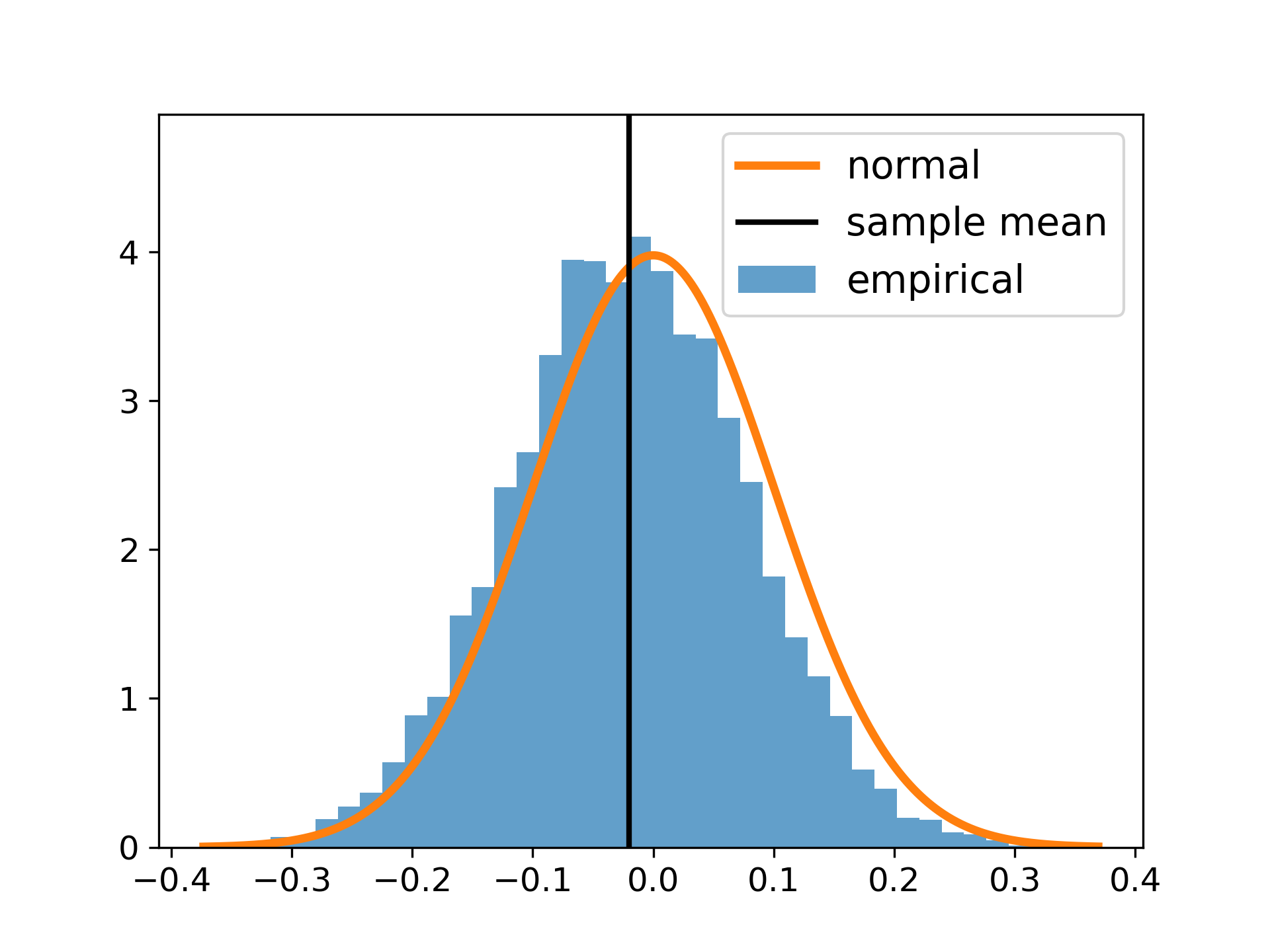
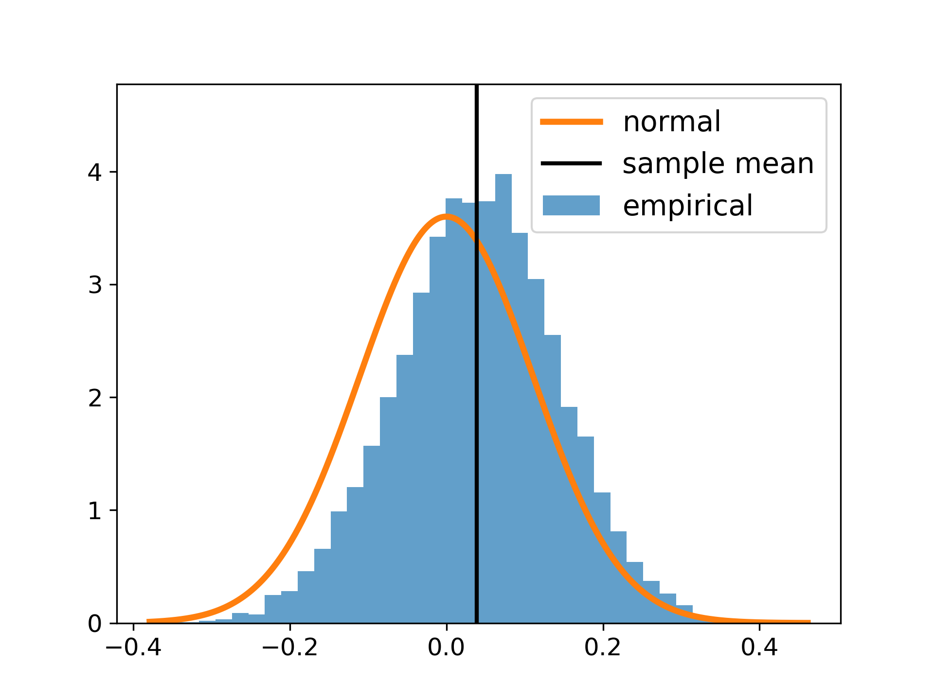
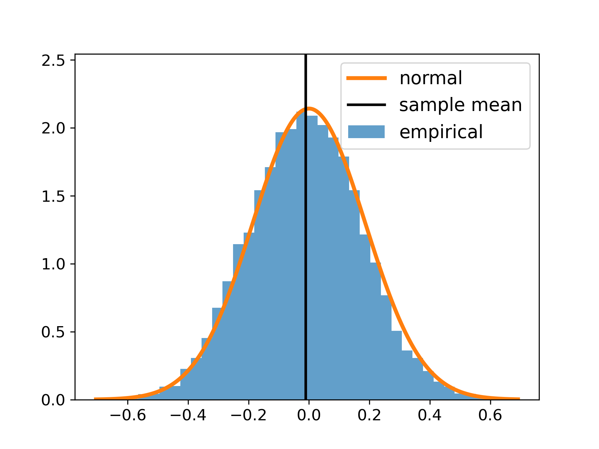
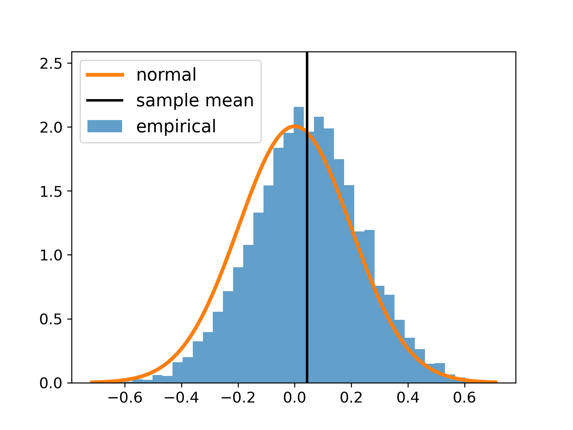
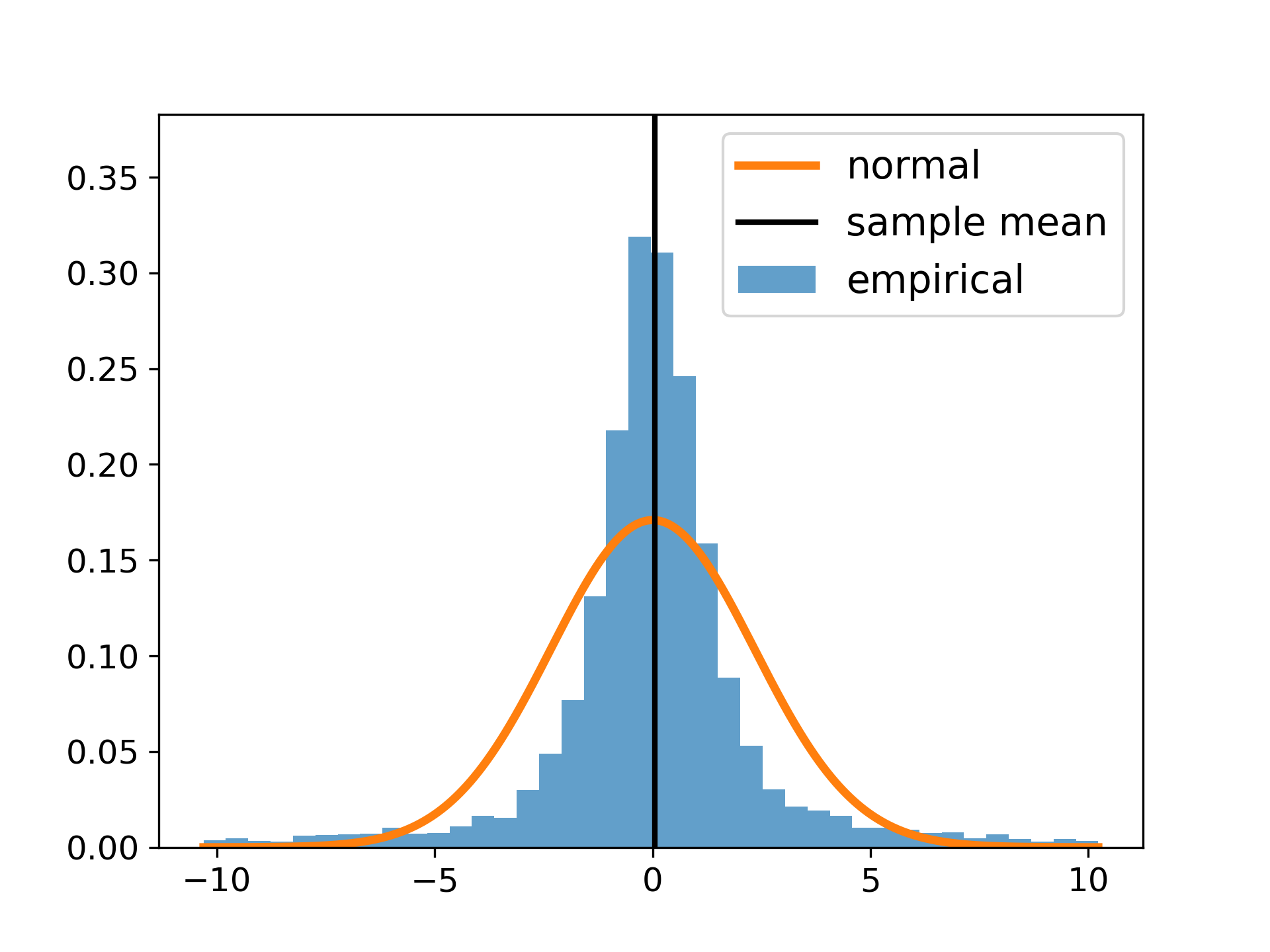
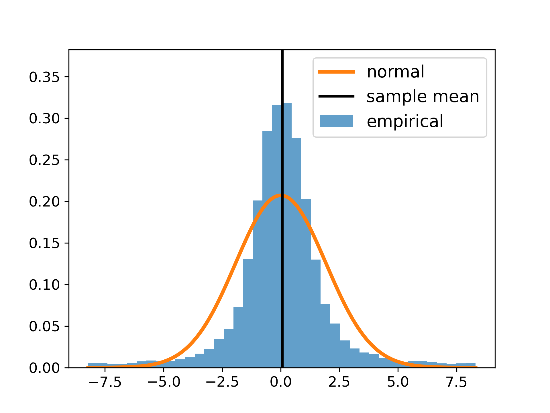
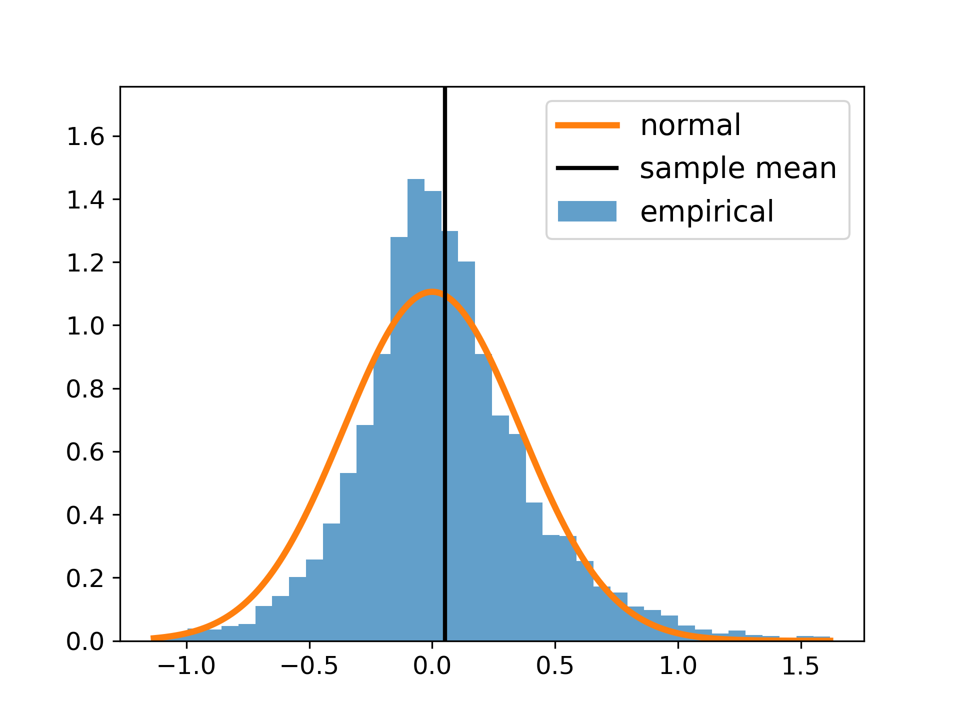
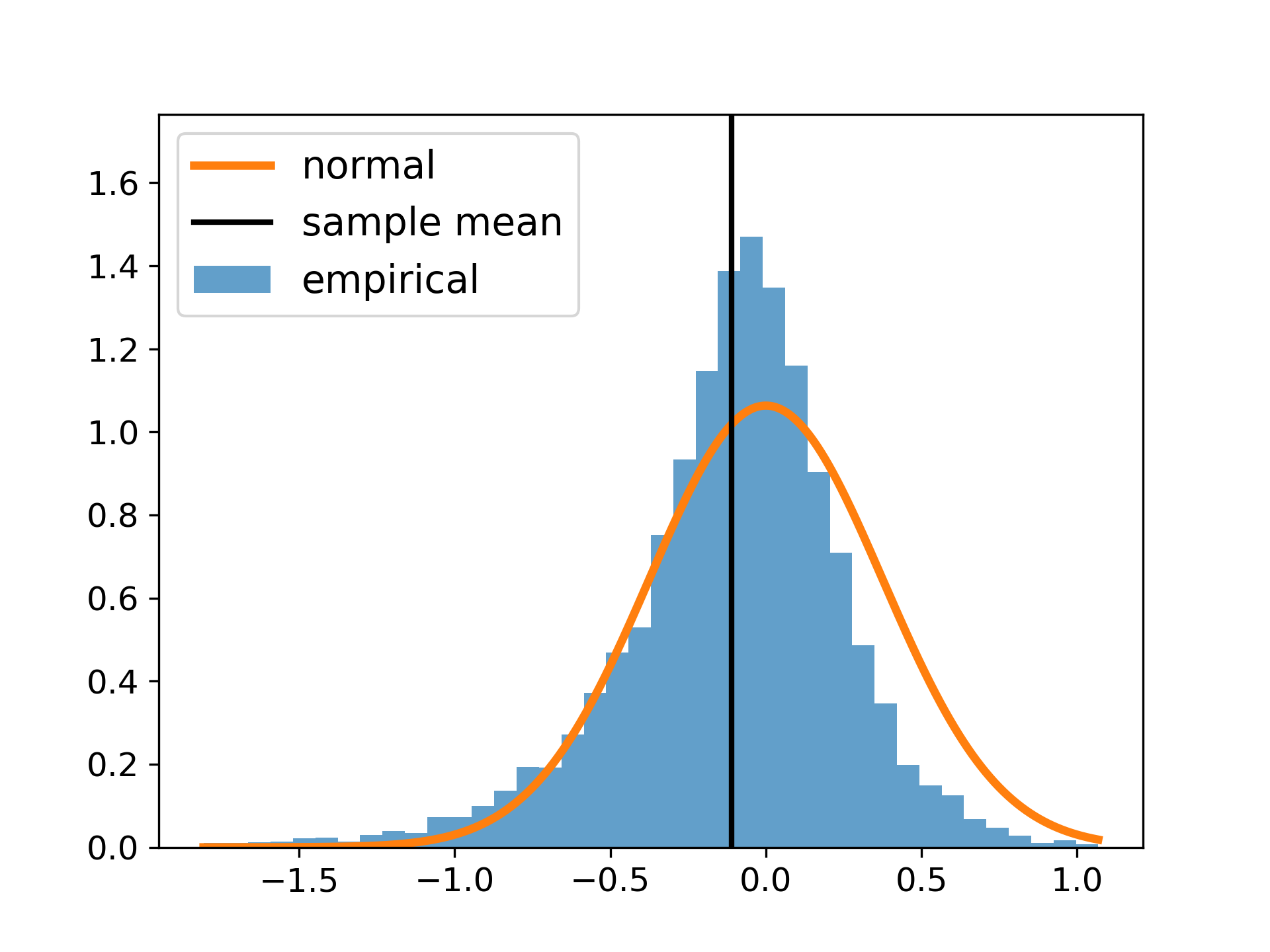
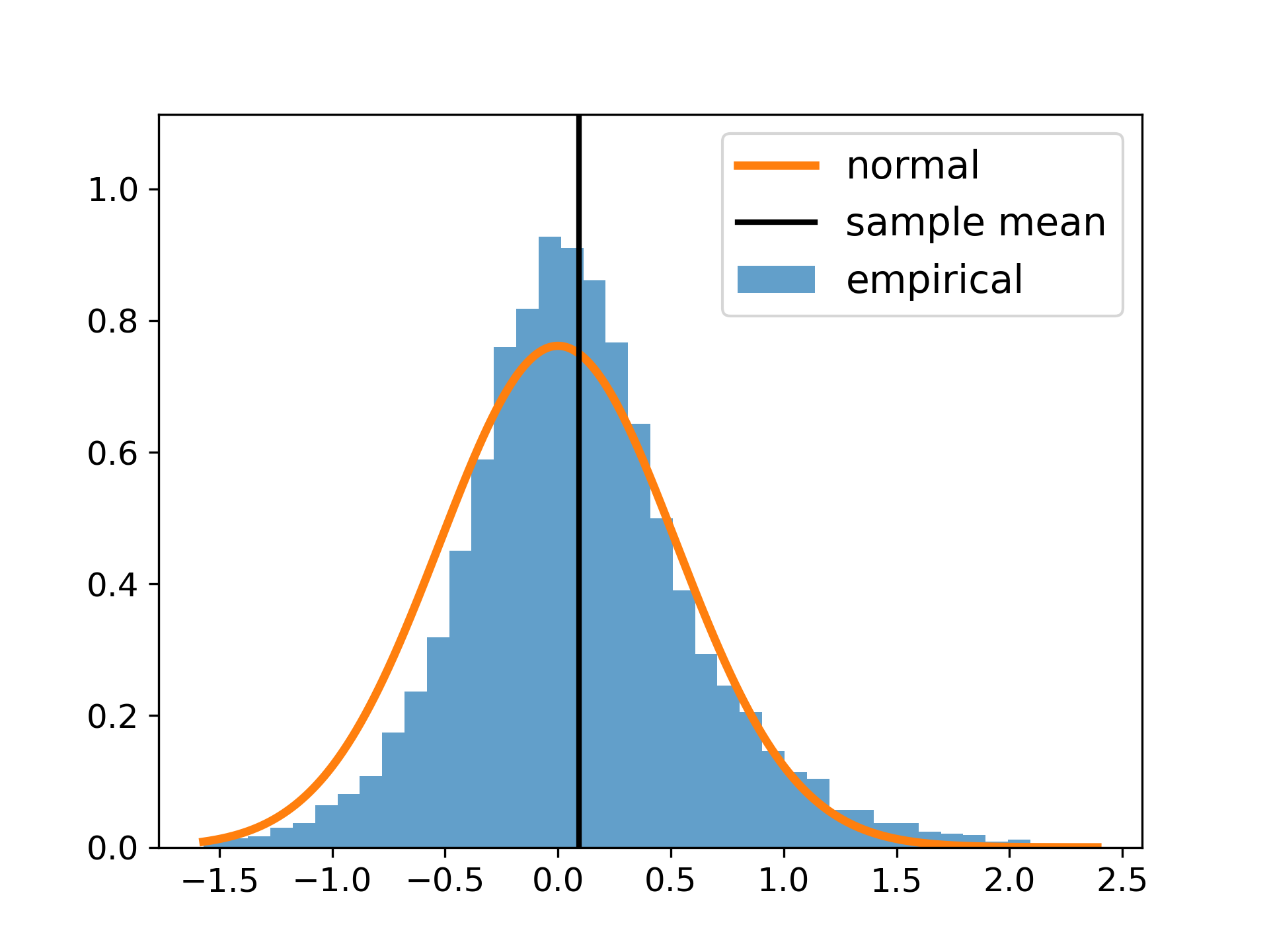
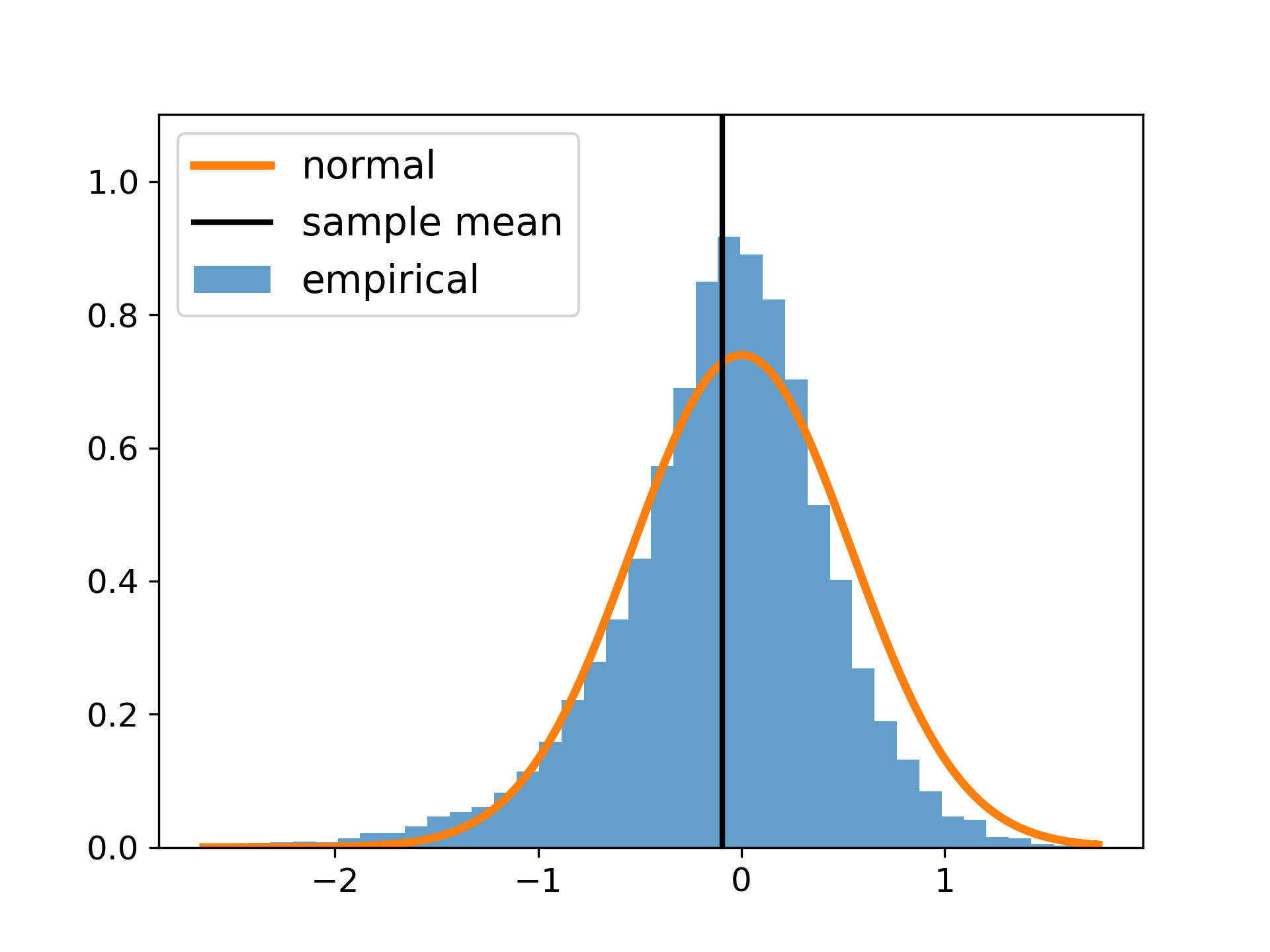
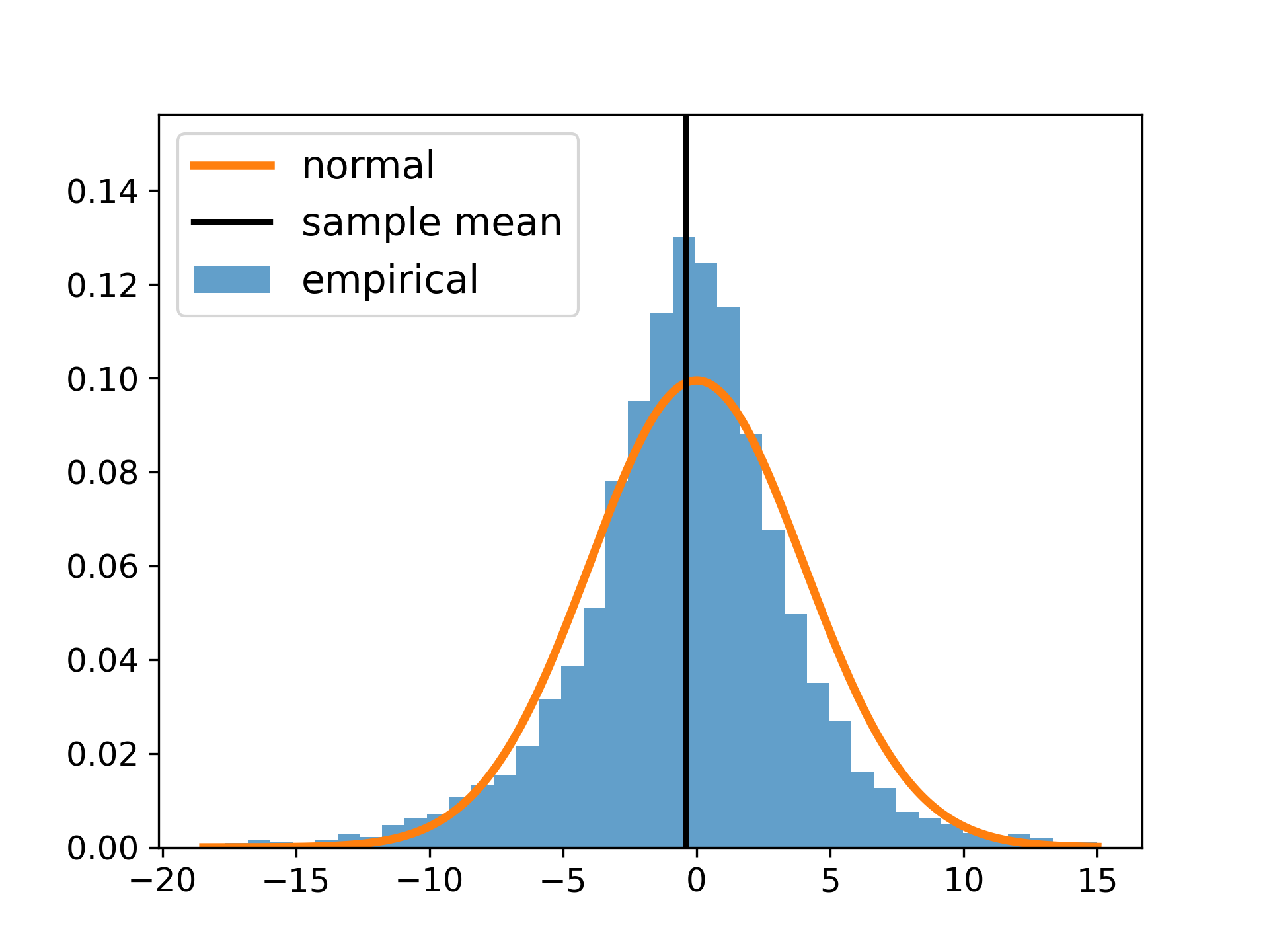
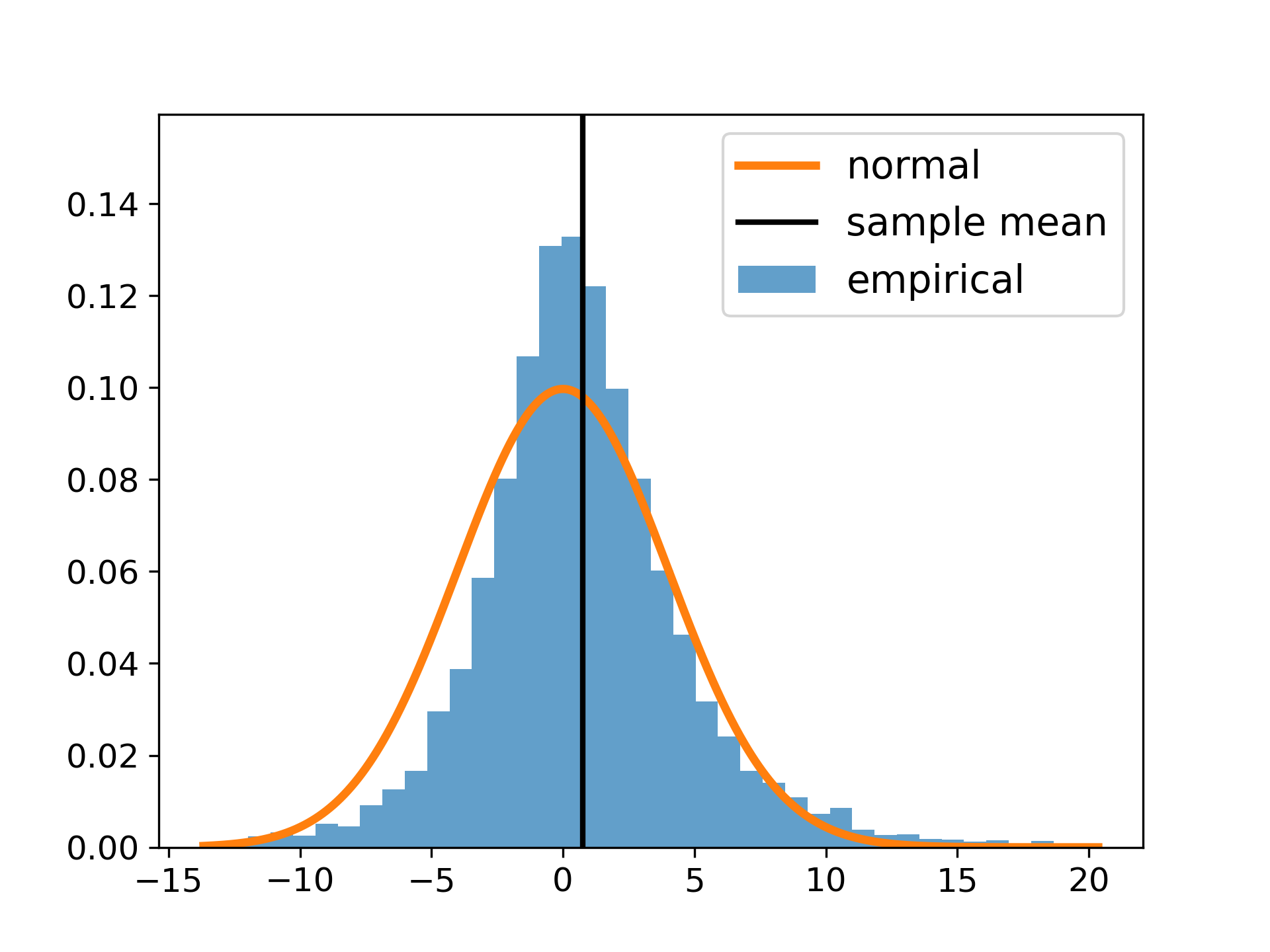
We first present the results for linear regression. In Figure 1, we plot the empirical distribution of $\sqrt{t}(\bar{\theta}_{t}-\theta^{*})$ using $10,000$ Monte-Carlo simulations. As can be inferred from the plots, the vanilla SGD and the square-root importance weight SGD have much smaller standard deviation compared with (IPW), this finding matches our discussion in Section 3. We also conduct simulations on quantile regression with quantile level $\tau=0.75$. The empirical distribution is reported in Figure 2.

5.2 Online statistical inference

In this section, we demonstrate the online plug-in inference procedure based on the limiting distribution of our proposed estimator $\bar{\theta}_{t}$ in Theorem 4.2. As we mentioned in the previous section, the plug-in estimator constructs a pair $(\widehat{S}_{n},\widehat{H}_{n})$ to estimate $(S,H)$ in the asymptotic covariance matrix $H^{-1}SH^{-1}$.

$\displaystyle\widehat{S}_{n}=\frac{1}{n}\sum_{t=1}^{n}w_{t}^{2}\nabla\ell(\theta_{t-1};\zeta_{t})\nabla\ell(\theta_{t-1};\zeta_{t})^{\top},\quad\widehat{H}_{n}=\frac{1}{n}\sum_{t=1}^{n}w_{t}\nabla^{2}\ell(\theta_{t-1};\zeta_{t}).$

Using linear regression as an example, we first establish the consistency of the plug-in estimator under the following additional assumption.

Assumption 6.

For any action $A\in\mathcal{A}$ and covariate $X$, we assume that $\nabla^{2}\ell(\theta;\zeta)$ exists and $\mathbb{E}_{\mathcal{P}_{Y\mid X}}\left(\|\nabla^{2}\ell(\theta;\zeta)\|^{2}\mid X,A\right)$ is bounded by $\psi(X)(1+\|\theta-\theta^{*}\|^{2})$ for some function $\psi(\cdot)$ such that $\mathbb{E}[\psi(X)]<\infty$. In addition, we have $\lim_{\theta\rightarrow\theta^{*}}\mathbb{E}_{\mathcal{P}_{X}}[\Delta(X,\theta)\psi(X)]=0$ where $\Delta(X,\theta)$ is defined in Assumption 4, and

$\displaystyle\lim_{\theta\rightarrow\theta^{*}}\mathbb{E}_{\mathcal{P}_{Y\mid X}}\left[\|\nabla^{2}\ell(\theta;\zeta)-\nabla^{2}\ell(\theta^{*};\zeta)\|^{2}\mid X,A\right]=0,\quad\lim_{\theta\rightarrow\theta^{*}}\mathbb{E}_{\mathcal{P}_{X}}\left[|w(\theta;X,A)-w(\theta^{*};X,A)|^{2}\psi(X)\mid A\right]=0.$
Proposition 5.1.

Under Assumption 1 to Assumption 6, the plug-in estimators are consistent, i.e., $\widehat{S}_{n}\to S$ and $\widehat{H}_{n}\to H$ in probability.

The proof is presented in Appendix E. Under the same setting as in Section 5.1, we show the inference results for linear regression in Table 1. The comparison of the three candidate weighted-SGD schemes is clearly stated. Both (vanilla)  and (sqrt-IPW)  provide a valid conference interval, while (IPW)  provides a much wider confidence interval than its oracle.

Weight & Arm Sample size Plug-in Cov. Oracle Cov. Plug-in Len. Oracle Len.
$2\times 10^{4}$ 0.78 (0.14) 0.73 (0.15) 0.63 (0.03) 0.55
(vanilla), Arm 0 $8\times 10^{4}$ 0.88 (0.09) 0.86 (0.09) 0.57 (0.01) 0.55
$2\times 10^{4}$ 0.89 (0.09) 0.83 (0.12) 0.63 (0.03 ) 0.55
(vanilla), Arm 1 $8\times 10^{4}$ 0.94 (0.07) 0.93 (0.08) 0.58 (0.01) 0.55
$2\times 10^{4}$ 0.78 (0.14) 0.72 (0.15) 0.82 (0.12) 0.72
(sqrt-IPW), Arm 0 $8\times 10^{4}$ 0.88 (0.10) 0.87 (0.11) 0.74 (0.04) 0.72
$2\times 10^{4}$ 0.84 (0.12) 0.78 (0.14) 0.83 (0.13) 0.72
(sqrt-IPW), Arm 1 $8\times 10^{4}$ 0.91 (0.09) 0.90 (0.10) 0.75 (0.05) 0.72
$2\times 10^{4}$ 0.81 (0.15) 0.47 (0.32) 19.18 (34.94) 2.79
(IPW), Arm 0 $8\times 10^{4}$ 0.85 (0.14) 0.62 (0.33) 13.04 (28.04) 2.79
$2\times 10^{4}$ 0.82 (0.15) 0.51 (0.32) 16.76 (32.12) 2.79
(IPW), Arm 1 $8\times 10^{4}$ 0.86 (0.13) 0.65 (0.32) 11.47 (25.80) 2.79
Table 1: Inference results of linear regression with different weighting schemes. Averaged coverage rate and average length of the confidence intervals are reported for plug-in estimator and oracle estimator. We also include standard error in the parentheses.

5.3 Real data analysis

In this section, we apply our online estimation and inference framework to Yahoo! Today module user click-log dataset and conduct statistical inference for model parameters. We use the news recommendation and user response records on May $1^{\mathrm{st}}$, 2009. On this day, we consider the two most recommended (recommended $405,888$ times) articles, No.109510 and No.109520 for analysis.

We follow the experiment settings in Chen, Lu and Song (2021b). The action $A_{t}$ is specified to be $1$ when Article No.109510 is recommended and $A_{t}=0$ when Article No.109520 is recommended. The original user features have six covariates, where the first five sum up to one, and the sixth is a constant $1$. In our experiments below, we keep the second to fifth covariates in the original features as $X_{[2:5]}$ and specify $X_{[1]}=1$ as the intercept.

As the reward $Y_{t}$ is binary, we consider a logistic regression model (Example 2.2) and set $Y_{t}=1$ if the user clicks on the article link and $Y_{t}=-1$ if not. We use the $\varepsilon$-greedy algorithm (8). In order to match our online decision-making process with our offline dataset, we keep the entry if the recorded offline action matches the action given by our online $\varepsilon$-greedy algorithm with two specifications of $\varepsilon\in\{0.2,0.02\}$.

Weight & Arm Parameter Estimate S.E. 95% LB 95% UB $t$-value $p$-value
$\theta_{1}$ -2.56 0.04 -2.64 -2.48 -65.52 0.00
$\theta_{2}$ -0.26 0.08 -0.43 -0.10 -3.11 0.00
$\theta_{3}$ -0.48 0.07 -0.62 -0.34 -6.80 0.00
$\theta_{4}$ -0.23 0.06 -0.34 -0.12 -4.09 0.00
(vanilla), Arm 0 $\theta_{5}$ -0.90 0.07 -1.03 -0.77 -13.65 0.00
$\theta_{6}$ -2.55 0.05 -2.65 -2.44 -47.77 0.00
$\theta_{7}$ -0.24 0.08 -0.40 -0.09 -3.06 0.00
$\theta_{8}$ -0.45 0.07 -0.58 -0.32 -6.76 0.00
$\theta_{9}$ -0.41 0.11 -0.62 -0.19 -3.71 0.00
(vanilla), Arm 1 $\theta_{10}$ -0.91 0.07 -1.05 -0.77 -12.31 0.00
$\theta_{1}$ -2.52 0.05 -2.62 -2.43 -52.85 0.00
$\theta_{2}$ -0.30 0.11 -0.51 -0.09 -2.79 0.01
$\theta_{3}$ -0.49 0.09 -0.66 -0.31 -5.56 0.00
$\theta_{4}$ -0.28 0.07 -0.4 -0.15 -4.25 0.00
(sqrt-IPW), Arm 0 $\theta_{5}$ -0.80 0.09 -0.97 -0.63 -9.33 0.00
$\theta_{6}$ -2.51 0.05 -2.61 -2.41 -49.35 0.00
$\theta_{7}$ -0.28 0.08 -0.43 -0.13 -3.60 0.00
$\theta_{8}$ -0.45 0.06 -0.58 -0.33 -7.10 0.00
$\theta_{9}$ -0.42 0.11 -0.63 -0.20 -3.83 0.00
(sqrt-IPW), Arm 1 $\theta_{10}$ -0.81 0.07 -0.94 -0.68 -12.02 0.00
$\theta_{1}$ -2.64 0.10 -2.85 -2.44 -25.54 0.00
$\theta_{2}$ -0.28 0.19 -0.64 0.08 -1.51 0.13
$\theta_{3}$ -0.51 0.15 -0.80 -0.23 -3.49 0.00
$\theta_{4}$ -0.24 0.16 -0.55 0.07 -1.54 0.12
(IPW), Arm 0 $\theta_{5}$ -0.91 0.16 -1.23 -0.59 -5.64 0.00
$\theta_{6}$ -2.47 0.03 -2.53 -2.40 -76.6 0.00
$\theta_{7}$ -0.22 0.06 -0.33 -0.11 -3.83 0.00
$\theta_{8}$ -0.51 0.05 -0.60 -0.42 -11.08 0.00
$\theta_{9}$ -0.37 0.05 -0.47 -0.27 -7.40 0.00
(IPW), Arm 1 $\theta_{10}$ -0.88 0.05 -0.98 -0.78 -17.67 0.00
Table 2: Real data analysis with online statistic inference. We use $\varepsilon$-greedy algorithm with $\varepsilon=0.2$.
Weight & Arm Parameter Estimate S.E. 95% LB 95% UB $t$-value $p$-value
$\theta_{1}$ -2.55 0.04 -2.63 -2.48 -68.62 0.00
$\theta_{2}$ -0.31 0.09 -0.47 -0.14 -3.61 0.00
$\theta_{3}$ -0.45 0.07 -0.6 -0.31 -6.18 0.00
$\theta_{4}$ -0.23 0.05 -0.33 -0.12 -4.29 0.00
(vanilla), Arm 0 $\theta_{5}$ -0.88 0.07 -1.01 -0.75 -13.45 0.00
$\theta_{6}$ -2.54 0.06 -2.66 -2.42 -41.76 0.00
$\theta_{7}$ -0.29 0.09 -0.45 -0.12 -3.36 0.00
$\theta_{8}$ -0.42 0.07 -0.57 -0.28 -5.88 0.00
$\theta_{9}$ -0.42 0.19 -0.79 -0.04 -2.18 0.03
(vanilla), Arm 1 $\theta_{10}$ -0.89 0.08 -1.04 -0.73 -11.25 0.00
$\theta_{1}$ -2.49 0.05 -2.58 -2.40 -54.74 0.00
$\theta_{2}$ -0.31 0.13 -0.57 -0.05 -2.37 0.02
$\theta_{3}$ -0.45 0.12 -0.68 -0.21 -3.74 0.00
$\theta_{4}$ -0.29 0.06 -0.41 -0.17 -4.78 0.00
(sqrt-IPW), Arm 0 $\theta_{5}$ -0.82 0.08 -0.98 -0.66 -9.80 0.00
$\theta_{6}$ -2.48 0.08 -2.64 -2.33 -31.13 0.00
$\theta_{7}$ -0.29 0.10 -0.50 -0.09 -2.84 0.00
$\theta_{8}$ -0.42 0.09 -0.60 -0.25 -4.69 0.00
$\theta_{9}$ -0.4 0.25 -0.90 0.09 -1.60 0.11
(sqrt-IPW), Arm 1 $\theta_{10}$ -0.82 0.10 -1.01 -0.63 -8.49 0.00
$\theta_{1}$ -2.75 0.33 -3.40 -2.11 -8.37 0.00
$\theta_{2}$ -0.22 0.57 -1.35 0.90 -0.39 0.70
$\theta_{3}$ -0.80 0.50 -1.78 0.18 -1.59 0.11
$\theta_{4}$ 0.11 0.39 -0.65 0.87 0.28 0.78
(IPW), Arm 0 $\theta_{5}$ -0.90 0.51 -1.89 0.09 -1.78 0.08
$\theta_{6}$ -2.40 0.09 -2.57 -2.23 -27.81 0.00
$\theta_{7}$ -0.33 0.14 -0.60 -0.07 -2.46 0.01
$\theta_{8}$ -0.33 0.08 -0.48 -0.17 -4.17 0.00
$\theta_{9}$ -0.55 0.30 -1.14 0.05 -1.81 0.07
(IPW), Arm 1 $\theta_{10}$ -1.14 0.20 -1.53 -0.76 -5.81 0.00
Table 3: Real data analysis with online statistic inference. We use $\varepsilon$-greedy algorithm with $\varepsilon=0.02$.

We now present the online statistical inference results. For our SGD update, we use the same settings as above experiments, i.e., $300$-step meltdown and $\alpha=0.8$. We compare three weighting schemes below, vanilla SGD (2), square-root importance weight SGD ((sqrt-IPW)), and IPW SGD ((IPW)). Table 2 below gives the result for $\varepsilon=0.2$ and Table 3 gives the result for $\varepsilon=0.02$. In both table, the vanilla SGD and the square-root importance SGD have smaller standard errors and smaller $p$-values. There are also more insignificant parameters for IPW SGD. The results of IPW SGD are worse when we decrease the value of $\varepsilon$, matches our findings in Theorem 4.2 and discussions in Section 3.

References

  • Bahadur (1966) Bahadur, R Raj (1966). A note on quantiles in large samples. The Annals of Mathematical Statistics 37(3), 577–580.
  • Ban and Rudin (2019) Ban, Gah-Yi and Cynthia Rudin (2019). The big data newsvendor: Practical insights from machine learning. Operations Research 67(1), 90–108.
  • Carroll (1978) Carroll, Raymond J (1978). On almost sure expansions for $m$-estimates. The Annals of Statistics 6(2), 314–318.
  • Chen, Song and Jordan (2022) Chen, Elynn Y, Rui Song, and Michael I Jordan (2022). Reinforcement learning with heterogeneous data: estimation and inference. arXiv preprint arXiv:2202.00088.
  • Chen, Lu and Song (2021a) Chen, Haoyu, Wenbin Lu, and Rui Song (2021a). Statistical inference for online decision making: In a contextual bandit setting. Journal of the American Statistical Association 116(533), 240–255.
  • Chen, Lu and Song (2021b) Chen, Haoyu, Wenbin Lu, and Rui Song (2021b). Statistical inference for online decision making via stochastic gradient descent. Journal of the American Statistical Association 116(534), 708–719.
  • Chen et al. (2020) Chen, Xi, Jason D Lee, Xin T Tong, and Yichen Zhang (2020). Statistical inference for model parameters in stochastic gradient descent. The Annals of Statistics 48(1), 251–273.
  • Chen et al. (2022) Chen, Xi, Zachary Owen, Clark Pixton, and David Simchi-Levi (2022). A statistical learning approach to personalization in revenue management. Management Science 68(3), 1923–1937.
  • Deshpande et al. (2018) Deshpande, Yash, Lester Mackey, Vasilis Syrgkanis, and Matt Taddy (2018). Accurate inference for adaptive linear models. In International Conference on Machine Learning, pp. 1194–1203. PMLR.
  • Duchi and Ruan (2021) Duchi, John C and Feng Ruan (2021). Asymptotic optimality in stochastic optimization. The Annals of Statistics 49(1), 21–48.
  • Fang, Xu and Yang (2018) Fang, Yixin, Jinfeng Xu, and Lei Yang (2018). Online bootstrap confidence intervals for the stochastic gradient descent estimator. The Journal of Machine Learning Research 19(1), 3053–3073.
  • Hammersley (2013) Hammersley, John (2013). Monte carlo methods. Springer Science & Business Media.
  • Hao et al. (2019) Hao, Botao, Yasin Abbasi Yadkori, Zheng Wen, and Guang Cheng (2019). Bootstrapping upper confidence bound. Advances in Neural Information Processing Systems 32.
  • He and Shao (1996) He, Xuming and Qi-Man Shao (1996). A general bahadur representation of M-estimators and its application to linear regression with nonstochastic designs. The Annals of Statistics 24(6), 2608–2630.
  • Kasy and Sautmann (2021) Kasy, Maximilian and Anja Sautmann (2021). Adaptive treatment assignment in experiments for policy choice. Econometrica 89(1), 113–132.
  • Khamaru et al. (2021) Khamaru, Koulik, Yash Deshpande, Lester Mackey, and Martin J Wainwright (2021). Near-optimal inference in adaptive linear regression. arXiv preprint arXiv:2107.02266.
  • Kim et al. (2011) Kim, Edward S, Roy S Herbst, Ignacio I Wistuba, J Jack Lee, George R Blumenschein, Anne Tsao, David J Stewart, Marshall E Hicks, Jeremy Erasmus, Sanjay Gupta, et al. (2011). The BATTLE trial: Personalizing therapy for lung cancerthe BATTLE trial: Personalizing therapy for lung cancer. Cancer Discovery 1(1), 44–53.
  • Langford and Zhang (2007) Langford, John and Tong Zhang (2007). The epoch-greedy algorithm for multi-armed bandits with side information. Advances in Neural Information Processing Systems 20.
  • Lee et al. (2022a) Lee, Sokbae, Yuan Liao, Myung Hwan Seo, and Youngki Shin (2022a). Fast and robust online inference with stochastic gradient descent via random scaling. In Proceedings of the AAAI Conference on Artificial Intelligence, Volume 36, pp.  7381–7389.
  • Lee et al. (2022b) Lee, Sokbae, Yuan Liao, Myung Hwan Seo, and Youngki Shin (2022b). Fast inference for quantile regression with millions of observations. arXiv preprint arXiv:2209.14502.
  • Li et al. (2010) Li, Lihong, Wei Chu, John Langford, and Robert E Schapire (2010). A contextual-bandit approach to personalized news article recoMendation. In Proceedings of the 19th international conference on World wide web, pp.  661–670.
  • Polyak and Juditsky (1992) Polyak, Boris T and Anatoli B Juditsky (1992). Acceleration of stochastic approximation by averaging. SIAM Journal on Control and Optimization 30(4), 838–855.
  • Qiang and Bayati (2016) Qiang, Sheng and Mohsen Bayati (2016). Dynamic pricing with demand covariates. arXiv preprint arXiv:1604.07463.
  • Ramprasad et al. (2022) Ramprasad, Pratik, Yuantong Li, Zhuoran Yang, Zhaoran Wang, Will Wei Sun, and Guang Cheng (2022). Online bootstrap inference for policy evaluation in reinforcement learning. Journal of the American Statistical Association, 1–14.
  • Robbins (1952) Robbins, Herbert (1952). Some aspects of the sequential design of experiments. Bulletin of the American Mathematical Society 58(5), 527–535.
  • Robbins and Monro (1951) Robbins, Herbert and Sutton Monro (1951). A stochastic approximation method. The Annals of Mathematical Statistics 22(3), 400–407.
  • Rockafellar and Uryasev (2002) Rockafellar, R Tyrrell and Stanislav Uryasev (2002). Conditional value-at-risk for general loss distributions. Journal of banking & finance 26(7), 1443–1471.
  • Ruppert (1988) Ruppert, David (1988). Efficient estimations from a slowly convergent robbins-monro process. Technical report, Cornell University Operations Research and Industrial Engineering.
  • Shao and Zhang (2022) Shao, Qi-Man and Zhuo-Song Zhang (2022). Berry–esseen bounds for multivariate nonlinear statistics with applications to M-estimators and stochastic gradient descent algorithms. Bernoulli 28(3), 1548–1576.
  • Shi et al. (2021) Shi, Chengchun, Shengxing Zhang, Wenbin Lu, and Rui Song (2021). Statistical inference of the value function for reinforcement learning in infinite-horizon settings. Journal of the Royal Statistical Society. Series B: Statistical Methodology.
  • Shi et al. (2022) Shi, Chengchun, Jin Zhu, Shen Ye, Shikai Luo, Hongtu Zhu, and Rui Song (2022). Off-policy confidence interval estimation with confounded markov decision process. Journal of the American Statistical Association, 1–12.
  • Su and Zhu (2018) Su, Weijie J and Yuancheng Zhu (2018). Uncertainty quantification for online learning and stochastic approximation via hierarchical incremental gradient descent. arXiv preprint arXiv:1802.04876.
  • Woodroofe (1979) Woodroofe, Michael (1979). A one-armed bandit problem with a concomitant variable. Journal of the American Statistical Association 74(368), 799–806.
  • Zhang, Janson and Murphy (2021) Zhang, Kelly, Lucas Janson, and Susan Murphy (2021). Statistical inference with M-estimators on adaptively collected data. Advances in Neural Information Processing Systems 34, 7460–7471.
  • Zhang, Janson and Murphy (2022) Zhang, Kelly W, Lucas Janson, and Susan A Murphy (2022). Statistical inference after adaptive sampling in non-markovian environments. arXiv preprint arXiv:2202.07098.
  • Zhu, Chen and Wu (2021) Zhu, Wanrong, Xi Chen, and Wei Biao Wu (2021). Online covariance matrix estimation in stochastic gradient descent. Journal of the American Statistical Association, 1–12.

Appendix A Proof of the general asymptotic normality result

Proof of Theorem 4.2

Proof.

By definition, the loss function can be written as

$\displaystyle\mathcal{L}_{\theta^{\prime}}(\theta)$ $\displaystyle=\mathbb{E}[w(\theta^{\prime};X,A^{\prime})\ell(\theta;Y,X,A^{\prime})]$
$\displaystyle=\mathbb{E}_{\mathcal{P}_{X},\pi(X,\theta^{\prime})}\left\{\mathbb{E}_{\mathcal{P}_{Y\mid X}}[w(\theta^{\prime};X,A^{\prime})\ell(\theta;Y,X,A^{\prime})]\mid X,A^{\prime}\right\}.$

By Equation (5), $\theta^{*}$ is the minimizer, i.e., $\theta^{*}\in\underset{\theta\in\mathbb{R}^{d}}{\operatorname{argmin}}\,\mathcal{L}_{\theta^{\prime}}(\theta)$. Because $\mathcal{L}$ is differentiable, We have $\nabla\mathcal{L}_{\theta^{\prime}}(\theta^{*})=0$. Moreover, we have

$\displaystyle\|\nabla\mathcal{L}_{\theta}(\theta)-H(\theta-\theta^{*})\|$ $\displaystyle=\left\|\nabla\mathcal{L}_{\theta}(\theta)-\nabla\mathcal{L}_{\theta}(\theta^{*})-H(\theta-\theta^{*})\right\|$
$\displaystyle=\left\|\int_{0}^{1}\left(\nabla^{2}\mathcal{L}_{\theta}(\theta^{*}+s(\theta-\theta^{*}))-H\right)(\theta-\theta^{*}){\,\mathrm{d}}s\right\|$
$\displaystyle\leq K\|\theta-\theta^{*}\|^{2},$ (A.1)

for $\|\theta-\theta^{*}\|<\delta$ as stated in Assumption 3.

By Equation (11), we have $w(\theta^{\prime};X,A)\nabla\ell(\theta;\zeta)=\xi_{\theta^{\prime}}(\theta;\zeta)+\nabla\mathcal{L}_{\theta^{\prime}}(\theta)$. Notice that we have the following inequality,

$\displaystyle\mathbb{E}[\|w(\theta;X,A)\nabla\ell(\theta;\zeta)\|^{2}]\leq\overline{w}^{2}\mathbb{E}[\nabla\ell(\theta;\zeta)^{2}]\leq\overline{w}^{2}\kappa(1+\|\theta-\theta^{*}\|^{2}).$

Therefore, by the fact that $\mathbb{E}[\xi_{\theta}(\theta;\zeta)]=0$, the two terms can be bounded by

$\displaystyle\left\|\nabla\mathcal{L}_{\theta}(\theta)\right\|^{2}$ $\displaystyle\leq\overline{w}^{2}\kappa(1+\|\theta-\theta^{*}\|^{2}),$
$\displaystyle\mathbb{E}\left[\|\xi_{\theta}(\theta;\zeta)\|^{2}\right]$ $\displaystyle\leq\overline{w}^{2}\kappa(1+\|\theta-\theta^{*}\|^{2}).$

The above bounds can already guarantee the almost surely convergence of $\theta_{t}$ by Theorem 2 of Polyak and Juditsky (1992). Now we need to quantify the difference between $\xi_{\theta_{t-1}}(\theta_{t-1};\zeta)$ and $\xi_{\theta^{*}}(\theta^{*};\zeta)$. Using the coupling we defined in Equation (13), it can be bounded by

$\displaystyle\mathbb{E}_{\mathcal{P},\nu}\|\xi_{\theta_{t-1}}(\theta_{t-1};\zeta)-\xi_{\theta^{*}}(\theta^{*};\zeta)\|^{2}$
$\displaystyle\leq\;$ $\displaystyle 2\|\nabla\mathcal{L}_{\theta_{t-1}}(\theta_{t-1})-\nabla\mathcal{L}_{\theta^{*}}(\theta^{*})\|^{2}+2\mathbb{E}_{\mathcal{P},\nu}\left[\|w(\theta_{t-1};X_{t},A_{t})\nabla\ell(\theta_{t-1};\zeta_{t})-w(\theta^{*};X_{t},A^{*})\nabla\ell(\theta^{*};X_{t},A^{*},Y_{t})\|^{2}\right]$
$\displaystyle:=$ $\displaystyle 2M_{1}+2M_{2}.$

From (A), we have the following bound for $M_{1}$,

$\displaystyle M_{1}\leq 2K^{2}\|\theta_{t-1}-\theta^{*}\|^{4}+2\|H\|_{2}^{2}\|\theta_{t-1}-\theta^{*}\|^{2}.$ (A.2)

Therefore, as $\theta_{t-1}$ converges to $\theta^{*}$, $M_{1}$ converges to 00.

The second term has the following inequality,

$\displaystyle M_{2}$ $\displaystyle\leq\mathbb{E}_{\mathcal{P}_{X}}\left[\Delta(X_{t},\theta_{t-1})M_{3}+(1-\Delta(X_{t},\theta_{t-1}))M_{4}\right],$ (A.3)

where

$\displaystyle M_{3}$ $\displaystyle:=\mathbb{E}_{\mathcal{P}_{Y\mid X},\nu}\left[\left\|w(\theta_{t-1};X_{t},A_{t})\nabla\ell(\theta_{t-1};X_{t},A_{t},Y_{t})-w(\theta^{*};X_{t},A^{*})\nabla\ell(\theta^{*};X_{t},A^{*},Y_{t})\right\|^{2}\mid X_{t},A_{t}\neq A^{*}\right],$
$\displaystyle M_{4}$ $\displaystyle:=\mathbb{E}_{\mathcal{P}_{Y\mid X},\nu}\left[\left\|w(\theta_{t-1};X_{t},A_{t})\nabla\ell(\theta_{t-1};X_{t},A_{t},Y_{t})-w(\theta^{*};X_{t},A^{*})\nabla\ell(\theta^{*};X_{t},A^{*},Y_{t})\right\|^{2}\mid X_{t},A_{t}=A^{*}\right].$

The third term $M_{3}$ can be bounded as,

$\displaystyle M_{3}$ $\displaystyle\leq 2\overline{w}^{2}\mathbb{E}_{\mathcal{P}_{Y\mid X},\nu}\left[\|\nabla\ell(\theta_{t-1};X_{t},A_{t},Y_{t})\|^{2}+\|\nabla\ell(\theta^{*};X_{t},A^{*},Y_{t})\|^{2}\mid X_{t},A_{t}\neq A^{*}\right]$
$\displaystyle\leq 4\overline{w}^{2}(1+\|\theta_{t-1}-\theta^{*}\|^{2})\phi(X_{t}).$ (A.4)

Finally, we have

$\displaystyle M_{4}$ $\displaystyle\leq\max_{A\in\mathcal{A}}\mathbb{E}_{\mathcal{P}_{Y\mid X}}\left[\|w(\theta_{t-1};X_{t},A)\nabla\ell(\theta_{t-1};X_{t},A,Y_{t})-w(\theta^{*};X_{t},A)\nabla\ell(\theta^{*};X_{t},A,Y_{t})\|^{2}\mid X_{t},A\right]$
$\displaystyle\leq 2\max_{A\in\mathcal{A}}\mathbb{E}_{\mathcal{P}_{Y\mid X}}\left[\|w(\theta_{t-1};X_{t},A)\nabla\ell(\theta_{t-1};X_{t},A,Y_{t})-w(\theta_{t-1};X_{t},A)\nabla\ell(\theta^{*};X_{t},A,Y_{t})\|^{2}\mid X_{t},A\right]$
$\displaystyle\quad+2\max_{A\in\mathcal{A}}\mathbb{E}_{\mathcal{P}_{Y\mid X}}\left[\|w(\theta_{t-1};X_{t},A)\nabla\ell(\theta^{*};X_{t},A,Y_{t})-w(\theta^{*};X_{t},A)\nabla\ell(\theta^{*};X_{t},A,Y_{t})\|^{2}\mid X_{t},A\right]$
$\displaystyle\leq 2\overline{w}^{2}\max_{A\in\mathcal{A}}\mathbb{E}_{\mathcal{P}_{Y\mid X}}\left[\|\nabla\ell(\theta_{t-1};X_{t},A,Y_{t})-\nabla\ell(\theta^{*};X_{t},A,Y_{t})\|^{2}\mid X_{t},A\right]$
$\displaystyle\quad+2\max_{A\in\mathcal{A}}|w(\theta_{t-1};X_{t},A)-w(\theta^{*};X_{t},A)|^{2}\phi(X_{t}).$ (A.5)

Combining (A) and (A) into (A.3), we have

$\displaystyle M_{2}$ $\displaystyle\leq\mathbb{E}_{\mathcal{P}_{X}}\left[\Delta(X_{t},\theta_{t-1})4\overline{w}^{2}(1+\|\theta_{t-1}-\theta^{*}\|^{2})\phi(X_{t})\right]$
$\displaystyle\quad+\mathbb{E}_{\mathcal{P}_{X}}\left[2\overline{w}^{2}\max_{A\in\mathcal{A}}\mathbb{E}_{\mathcal{P}_{Y|X}}[\|\nabla\ell(\theta_{t-1};X_{t},A,Y_{t})-\nabla\ell(\theta^{*};X_{t},A,Y_{t})\|^{2}\mid X_{t},A]\right]$
$\displaystyle\quad+\mathbb{E}_{\mathcal{P}_{X}}\left[2\max_{A\in\mathcal{A}}|w(\theta_{t-1};X_{t},A)-w(\theta^{*};X_{t},A)|^{2}\phi(X_{t})\right].$ (A.6)

Using Assumption 5, when $\theta_{t-1}\rightarrow\theta^{*}$, we have $M_{2}$ converges to 00.

We can now conclude from our above results that

$\displaystyle\lim_{\theta_{t}\rightarrow\theta^{*}}\mathbb{E}\|\xi_{\theta_{t-1}}(\theta_{t-1};\zeta)-\xi_{\theta^{*}}(\theta^{*};\zeta)\|^{2}=0.$

Note that all three conditions in Theorem 2 of Polyak and Juditsky (1992) are verified under our assumptions, we can conclude that the asymptotic normality result holds in Theorem 4.2. ∎

Appendix B Proof of Results in Linear Regression and Quantile Regression

Proof of Corollary 4.3

Proof.

Now let’s compute $\mathcal{L}_{\theta^{\prime}}(\theta)$, under $\varepsilon$-greedy policy defined in (8),

$\displaystyle\mathcal{L}_{\theta^{\prime}}(\theta)$ $\displaystyle=\frac{1}{2}\mathbb{E}_{\mathcal{P}}\left\{\mathbb{E}_{\pi(X,\theta^{\prime})}\left[\varphi(\mathbb{P}(A\mid X,\theta^{\prime}\,))\left((1-A)(Y-X^{\top}\theta_{[1:p]})^{2}+A(Y-X^{\top}\theta_{[p+1:2p]})^{2}\right)\mid X\right]\right\}$
$\displaystyle=\frac{1}{2}(1-\frac{\varepsilon}{2})\varphi(1-\frac{\varepsilon}{2})\mathbb{E}_{\mathcal{P}_{X}}\left[\mathbbm{1}\{X^{\top}\theta^{\prime}_{[1:p]}>X^{\top}\theta^{\prime}_{[p+1:2p]}\}\left(X^{\top}\theta^{*}_{[1:p]}-X^{\top}\theta_{[1:p]}\right)^{2}\right]$
$\displaystyle\quad+\frac{\varepsilon}{4}\varphi(\frac{\varepsilon}{2})\mathbb{E}_{\mathcal{P}_{X}}\left[\mathbbm{1}\{X^{\top}\theta^{\prime}_{[1:p]}>X^{\top}\theta^{\prime}_{[p+1:2p]}\}\left(X^{\top}\theta^{*}_{[p+1:2p]}-X^{\top}\theta_{[p+1:2p]}\right)^{2}\right]$
$\displaystyle\quad+\frac{\varepsilon}{4}\varphi(\frac{\varepsilon}{2})\mathbb{E}_{\mathcal{P}_{X}}\left[\mathbbm{1}\{X^{\top}\theta^{\prime}_{[1:p]}<X^{\top}\theta^{\prime}_{[p+1:2p]}\}\left(X^{\top}\theta^{*}_{[1:p]}-X^{\top}\theta_{[1:p]}\right)^{2}\right]$
$\displaystyle\quad+\frac{1}{2}(1-\frac{\varepsilon}{2})\varphi(1-\frac{\varepsilon}{2})\mathbb{E}_{\mathcal{P}_{X}}\left[\mathbbm{1}\{X^{\top}\theta^{\prime}_{[1:p]}<X^{\top}\theta^{\prime}_{[p+1:2p]}\}\left(X^{\top}\theta^{*}_{[p+1:2p]}-X^{\top}\theta_{[p+1:2p]}\right)^{2}\right]$
$\displaystyle\quad+\sigma^{2}\left[\frac{1}{2}(1-\frac{\varepsilon}{2})\varphi(1-\frac{\varepsilon}{2})+\frac{\varepsilon}{4}\varphi(\frac{\varepsilon}{2})\right].$ (B.1)

Obviously, the first part of Assumption 2 is satisfied under this form of loss function $\mathcal{L}$.

Also, we can calculate the gradient of $\mathcal{L}$ with respect to $\theta$ as follows,

$\displaystyle\nabla_{[1:p]}\mathcal{L}_{\theta^{\prime}}(\theta)$ $\displaystyle=(1-\frac{\varepsilon}{2})\varphi(1-\frac{\varepsilon}{2})\mathbb{E}_{\mathcal{P}_{X}}\left[\mathbbm{1}\{X^{\top}\theta^{\prime}_{[1:p]}>X^{\top}\theta^{\prime}_{[p+1:2p]}\}XX^{\top}\left(\theta_{[1:p]}-\theta^{*}_{[1:p]}\right)\right]$
$\displaystyle\quad+\frac{\varepsilon}{2}\varphi(\frac{\varepsilon}{2})\mathbb{E}_{\mathcal{P}_{X}}\left[\mathbbm{1}\{X^{\top}\theta^{\prime}_{[1:p]}<X^{\top}\theta^{\prime}_{[p+1:2p]}\}XX^{\top}\left(\theta_{[1:p]}-\theta^{*}_{[1:p]}\right)\right]$
$\displaystyle\nabla_{[p+1:2p]}\mathcal{L}_{\theta^{\prime}}(\theta)$ $\displaystyle=\frac{\varepsilon}{2}\varphi(\frac{\varepsilon}{2})\mathbb{E}_{\mathcal{P}_{X}}\left[\mathbbm{1}\{X^{\top}\theta^{\prime}_{[1:p]}>X^{\top}\theta^{\prime}_{[p+1:2p]}\}XX^{\top}\left(\theta_{[p+1:2p]}-\theta^{*}_{[p+1:2p]}\right)\right]$
$\displaystyle\quad+(1-\frac{\varepsilon}{2})\varphi(1-\frac{\varepsilon}{2})\mathbb{E}_{\mathcal{P}_{X}}\left[\mathbbm{1}\{X^{\top}\theta^{\prime}_{[1:p]}<X^{\top}\theta^{\prime}_{[p+1:2p]}\}XX^{\top}\left(\theta_{[p+1:2p]}-\theta^{*}_{[p+1:2p]}\right)\right].$

Therefore, the second part of Assumption 2 is naturally satisfied since we have the following,

$\displaystyle\langle\nabla\mathcal{L}_{\theta}(\theta),\theta-\theta^{*}\rangle\geq\min\left\{(1-\frac{\varepsilon}{2})\varphi(1-\frac{\varepsilon}{2}),\frac{\varepsilon}{2}\varphi(\frac{\varepsilon}{2})\right\}\,\mathbb{E}_{\mathcal{P}_{X}}[XX^{\top}]\left[\left(\theta_{[1:p]}-\theta^{*}_{[1:p]}\right)^{2}+\left(\theta_{[p+1:2p]}-\theta^{*}_{[p+1:2p]}\right)^{2}\right].$

We now consider the Hessian matrix, we have

$\displaystyle\nabla^{2}\mathcal{L}_{\theta^{\prime}}(\theta)=\begin{bmatrix}H_{1}&0\\ 0&H_{2}\end{bmatrix},$

where

$\displaystyle H_{1}$ $\displaystyle=(1-\frac{\varepsilon}{2})\varphi(1-\frac{\varepsilon}{2})\mathbb{E}_{\mathcal{P}_{X}}\left[\mathbbm{1}\{X^{\top}\theta^{\prime}_{[1:p]}>X^{\top}\theta^{\prime}_{[p+1:2p]}\}XX^{\top}\right]$
$\displaystyle\quad+\frac{\varepsilon}{2}\varphi(\frac{\varepsilon}{2})\mathbb{E}_{\mathcal{P}_{X}}\left[\mathbbm{1}\{X^{\top}\theta^{\prime}_{[1:p]}<X^{\top}\theta^{\prime}_{[p+1:2p]}\}XX^{\top}\right]$
$\displaystyle H_{2}$ $\displaystyle=\frac{\varepsilon}{2}\varphi(\frac{\varepsilon}{2})\mathbb{E}_{\mathcal{P}_{X}}\left[\mathbbm{1}\{X^{\top}\theta^{\prime}_{[1:p]}>X^{\top}\theta^{\prime}_{[p+1:2p]}\}XX^{\top}\right]$
$\displaystyle\quad+(1-\frac{\varepsilon}{2})\varphi(1-\frac{\varepsilon}{2})\mathbb{E}_{\mathcal{P}_{X}}\left[\mathbbm{1}\{X^{\top}\theta^{\prime}_{[1:p]}<X^{\top}\theta^{\prime}_{[p+1:2p]}\}XX^{\top}\right].$

Obviously, the Hessian matrix exists for all $(\theta,\theta^{\prime})\in\mathbb{R}^{d}\times\mathbb{R}^{d}$, and the Hessian matrix at $(\theta^{*};\theta^{*})$ is positive definite since $\lambda_{\min}\mathbb{E}_{\mathcal{P}_{X}}[XX^{\top}]>0$. We now check the Lipschitz continuity of $\nabla^{2}\mathcal{L}_{\theta^{\prime}}(\theta)$ at $(\theta^{*},\theta^{*})$. It is a constant function with respect to $\theta$, so we only need to consider its Lipschitz continuity with respect to $\theta^{\prime}$.

For a smooth integrable function $p(x)$, define the function $J(\theta)=\int\mathbbm{1}(\theta^{\top}x>c)p(x){\,\mathrm{d}}x$. It is easy to see that

$\displaystyle\nabla J(\theta)=\int_{\theta^{\top}x=c}p(x)x{\,\mathrm{d}}x.$

Apply this formula to $H_{1}$ and $H_{2}$, we get

$\displaystyle\quad\frac{\partial}{\partial\theta_{[1:p]}^{\prime}}H_{1}=-\frac{\partial}{\partial\theta_{[p+1:2p]}^{\prime}}H_{1}=-\frac{\partial}{\partial\theta_{[1:p]}^{\prime}}H_{2}=\frac{\partial}{\partial\theta_{[p+1:2p]}^{\prime}}H_{2}$ (B.2)
$\displaystyle=\left((1-\frac{\varepsilon}{2})p(1-\frac{\varepsilon}{2})-\frac{\varepsilon}{2}p(\frac{\varepsilon}{2})\right)\int_{x^{\top}\theta^{\prime}_{[1:p]}=x^{\top}\theta^{\prime}_{[p+1:2p]}}x\otimes x\otimes xp(x){\,\mathrm{d}}x.$ (B.3)

So $\nabla^{2}\mathcal{L}_{\theta^{\prime}}(\theta)$ is Lipschitz continuous at $(\theta^{*},\theta^{*})$ as long as $\int_{x^{\top}\theta^{*}_{[1:p]}=x^{\top}\theta^{*}_{[p+1:2p]}}x\otimes x\otimes xp(x){\,\mathrm{d}}x$ exists. Therefore, we verify Assumption 3.

For any $A,X$, we can bound

$\displaystyle\mathbb{E}_{\mathcal{P}_{Y\mid X}}(\|\nabla\ell(\theta;\zeta)\|^{2}\mid X,A)$ $\displaystyle\leq\|X\|^{2}\sigma^{2}+\|XX^{\top}XX^{\top}\|\|\theta-\theta^{*}\|^{2}.$

The matrix $S$ can be computed by

$\displaystyle S=\mathbb{E}[\nabla\ell(\theta;\zeta)\nabla\ell(\theta;\zeta)^{\top}]:=\begin{bmatrix}S_{1}&0\\ 0&S_{2}\end{bmatrix},$

where

$\displaystyle S_{1}$ $\displaystyle=(1-\frac{\varepsilon}{2})\varphi^{2}(1-\frac{\varepsilon}{2})\sigma^{2}\mathbb{E}_{\mathcal{P}_{X}}\left[\mathbbm{1}\{X^{\top}\theta^{*}_{[1:p]}>X^{\top}\theta^{*}_{[p+1:2p]}\}XX^{\top}\right]$
$\displaystyle\quad+\frac{\varepsilon}{2}\varphi^{2}(\frac{\varepsilon}{2})\sigma^{2}\mathbb{E}_{\mathcal{P}_{X}}\left[\mathbbm{1}\{X^{\top}\theta^{*}_{[1:p]}<X^{\top}\theta^{*}_{[p+1:2p]}\}XX^{\top}\right],$
$\displaystyle S_{2}$ $\displaystyle=(1-\frac{\varepsilon}{2})\varphi^{2}(1-\frac{\varepsilon}{2})\sigma^{2}\mathbb{E}_{\mathcal{P}_{X}}\left[\mathbbm{1}\{X^{\top}\theta^{*}_{[1:p]}<X^{\top}\theta^{*}_{[p+1:2p]}\}XX^{\top}\right]$
$\displaystyle\quad+\frac{\varepsilon}{2}\varphi^{2}(\frac{\varepsilon}{2})\sigma^{2}\mathbb{E}_{\mathcal{P}_{X}}\left[\mathbbm{1}\{X^{\top}\theta^{*}_{[1:p]}>X^{\top}\theta^{*}_{[p+1:2p]}\}XX^{\top}\right].$

So Assumption 4 is satisfied with $\phi(X)=\|X\|^{2}\sigma^{2}+\|XX^{\top}\|^{2}$.

By definition

$\displaystyle\Delta(X,\theta)=(1-\varepsilon)\left|\mathbbm{1}\left(X^{\top}\theta^{*}_{[1:p]}>X^{\top}\theta^{*}_{[p+1:2p]}\right)-\mathbbm{1}\left(X^{\top}\theta_{[1:p]}>X^{\top}\theta_{[p+1:2p]}\right)\right|.$

Take any convergent sequence $\theta_{n}\rightarrow\theta^{*}$. It is clear that $\Delta(X,\theta_{n})\phi(X)$ converges to 0 almost surely. Furthermore, $|\Delta(X,\theta_{n})\phi(X)|\leq\|X\|^{4}$ and $\mathbb{E}\|X\|^{4}\leq\infty$. By dominated convergence theorem, $\lim_{n\rightarrow\infty}\mathbb{E}[\Delta(X,\theta_{n})\phi(X)]=0$.

$\displaystyle\quad|w(\theta_{t-1};X_{t},A)-w(\theta^{*};X_{t},A)|$
$\displaystyle=|\varphi(\mathbb{P}(A_{t}|X_{t};\theta_{t-1}))-\varphi(\mathbb{P}(A|X_{t};\theta^{*}))|$
$\displaystyle=|\varphi(1-\frac{\varepsilon}{2})-\varphi(\frac{\varepsilon}{2})|\left|\mathbbm{1}\left(X^{\top}\theta^{*}_{[1:p]}>X^{\top}\theta^{*}_{[p+1:2p]}\right)-\mathbbm{1}\left(X^{\top}\theta_{[1:p]}>X^{\top}\theta_{[p+1:2p]}\right)\right|.$

Using the same argument as above, we can derive that

$\displaystyle\lim_{\theta\rightarrow\theta^{*}}\mathbb{E}_{\mathcal{P}_{X}}\left[|w(\theta;X,A)-w(\theta^{*};X,A)|^{2}\phi(X)\mid A\right]=0.$

Finally, we have the following inequality,

$\displaystyle\mathbb{E}_{\mathcal{P}}\left[\|\nabla\ell(\theta;\zeta)-\nabla\ell(\theta^{*};\zeta)\|^{2}\mid A\right]\leq\mathbb{E}_{\mathcal{P}_{X}}\left\|XX^{\top}(\theta-\theta^{*})\right\|^{2}.$

Therefore, Assumption 5 is satisfied since

$\displaystyle\lim_{\theta\rightarrow\theta^{*}}\mathbb{E}_{\mathcal{P}}\left[\|\nabla\ell(\theta;\zeta)-\nabla\ell(\theta^{*};\zeta)\|^{2}\mid A\right]=0.$

Proof of Theorem 3.1

Theorem 3.1 follows directly from Remark 4.1 and Corollary 4.3.

Explicit forms of the eigenvalues of $H^{-1}SH^{-1}$ in (9).

We can write $H^{-1}SH^{-1}$ as follows,

$\displaystyle H^{-1}SH^{-1}=\sigma^{2}\begin{bmatrix}c_{1}I+c_{2}\nu^{*}\nu^{*\top}&0\\ 0&c_{3}I+c_{4}\nu^{*}\nu^{*\top}\end{bmatrix},$ (B.4)

where

$\displaystyle c_{1}$ $\displaystyle=\frac{(1-\frac{\varepsilon}{2})^{1+2\gamma}\Phi(a)+(\frac{\varepsilon}{2})^{1+2\gamma}(1-\Phi(a))}{((1-\frac{\varepsilon}{2})^{1+\gamma}\Phi(a)+(\frac{\varepsilon}{2})^{1+\gamma}(1-\Phi(a)))^{2}},$
$\displaystyle c_{2}$ $\displaystyle=\frac{(1-\frac{\varepsilon}{2})^{1+2\gamma}(\Phi(a)+\frac{1}{\sqrt{2\pi}}ae^{\frac{a^{2}}{2}})+(\frac{\varepsilon}{2})^{1+2\gamma}(1-\Phi(a)-\frac{1}{\sqrt{2\pi}}ae^{\frac{a^{2}}{2}})}{((1-\frac{\varepsilon}{2})^{1+\gamma}(\Phi(a)+\frac{1}{\sqrt{2\pi}}ae^{\frac{a^{2}}{2}})+(\frac{\varepsilon}{2})^{1+\gamma}(1-\Phi(a)-\frac{1}{\sqrt{2\pi}}ae^{\frac{a^{2}}{2}}))^{2}}-c_{1},$
$\displaystyle c_{3}$ $\displaystyle=\frac{(1-\frac{\varepsilon}{2})^{1+2\gamma}(1-\Phi(a))+(\frac{\varepsilon}{2})^{1+2\gamma}\Phi(a)}{((1-\frac{\varepsilon}{2})^{1+\gamma}(1-\Phi(a))+(\frac{\varepsilon}{2})^{1+\gamma}\Phi(a))^{2}},$
$\displaystyle c_{4}$ $\displaystyle=\frac{(1-\frac{\varepsilon}{2})^{1+2\gamma}(1-\Phi(a)-\frac{1}{\sqrt{2\pi}}ae^{\frac{a^{2}}{2}})+(\frac{\varepsilon}{2})^{1+2\gamma}(\Phi(a)+\frac{1}{\sqrt{2\pi}}ae^{\frac{a^{2}}{2}})}{((1-\frac{\varepsilon}{2})^{1+\gamma}(1-\Phi(a)-\frac{1}{\sqrt{2\pi}}ae^{\frac{a^{2}}{2}})+(\frac{\varepsilon}{2})^{1+\gamma}(\Phi(a)+\frac{1}{\sqrt{2\pi}}ae^{\frac{a^{2}}{2}}))^{2}}-c_{3}.$

The eigenvalues of the asymptotic covariance matrix are $c_{1},c_{1}+c_{2},c_{3},c_{3}+c_{4}$ in the above equations.

Proof of Corollary 3.2

Proof.

Consider a $k$-arm bandit linear regression setting. Our central limit theorem gives the covariance of the form

$\displaystyle\Sigma=H^{-1}SH^{-1},$

where

$\displaystyle H=\nabla^{2}\mathcal{L}_{\theta^{*}}(\theta^{*})=\mathbb{E}[w(\theta^{*})\nabla^{2}\ell(\theta^{*})],$

and

$\displaystyle S=\mathbb{E}[\xi_{\theta^{*}}(\theta^{*};\zeta)\xi_{\theta^{*}}(\theta^{*};\zeta)^{\top}]=\mathbb{E}[(w(\theta^{*})^{2}\nabla\ell(\theta^{*})\nabla\ell(\theta^{*})^{\top}].$

One special property of linear regression is that

$\displaystyle\nabla^{2}\ell(\theta^{*})^{2}=(X_{t}X_{t}^{\top})\otimes E_{i},$

where $E_{k}$ is the matrix with 1 on the $(k,k)$ entry and other entries to be 0, $i$ means we choose the $i$-th bandit, and

$\displaystyle(\nabla\ell(\theta^{*}))(\nabla\ell(\theta^{*}))^{\top}=(X_{t}X_{t}^{\top})\otimes E_{i}\mathbb{E}\sigma^{2}.$

So they differ only by a constant factor. If $w$ is constant instead of stochastic, we denote the corresponding $H,S,\Sigma$ as $H_{c},S_{c},\Sigma_{c}$. We claim that $\Sigma\succeq\Sigma_{c}$. Equal weight is optimal for linear regression. This is equivalent to

$\displaystyle(\mathbb{E}[w(\theta^{*})\nabla^{2}\ell(\theta^{*})])^{-1}(\mathbb{E}[w(\theta^{*})^{2}\nabla^{2}\ell(\theta^{*})])(\mathbb{E}[w(\theta^{*})\nabla^{2}\ell(\theta^{*})])^{-1}\succeq(\mathbb{E}[\nabla^{2}\ell(\theta^{*})])^{-1},$

which is the same as

$\displaystyle\mathbb{E}[w(\theta^{*})^{2}\nabla^{2}\ell(\theta^{*})]-(\mathbb{E}[w(\theta^{*})\nabla^{2}\ell(\theta^{*})])(\mathbb{E}[\nabla^{2}\ell(\theta^{*})])^{-1}(\mathbb{E}[w(\theta^{*})\nabla^{2}\ell(\theta^{*})])\succeq 0.$

By Schur complement, this is equivalent to

$\displaystyle\begin{bmatrix}\mathbb{E}[w(\theta^{*})^{2}\nabla^{2}\ell(\theta^{*})]&\mathbb{E}[w(\theta^{*})\nabla^{2}\ell(\theta^{*})]\\ \mathbb{E}[w(\theta^{*})\nabla^{2}\ell(\theta^{*})]&\mathbb{E}[\nabla^{2}\ell(\theta^{*})]\end{bmatrix}\succeq 0.$

Note that

$\displaystyle\begin{bmatrix}w(\theta^{*})^{2}\nabla^{2}\ell(\theta^{*})&w(\theta^{*})\nabla^{2}\ell(\theta^{*})\\ w(\theta^{*})\nabla^{2}\ell(\theta^{*})&\nabla^{2}\ell(\theta^{*})\end{bmatrix}\succeq 0.$

Therefore, our conclusion holds.

Proof of Corollary 4.4

Proof.

We first define $\psi_{\tau}(u)$ as follows,

$\displaystyle\psi_{\tau}(u)=\mathbb{E}_{\mathcal{E}}\rho_{\tau}(u+\mathcal{E})=\int_{-\infty}^{-u}(u+x)(\tau-1)q(x){\,\mathrm{d}}x+\int_{-u}^{\infty}(u+x)\tau q(x){\,\mathrm{d}}x.$

The first and second order derivative of $\psi_{\tau}(u)$ can be computed as

$\displaystyle\psi^{\prime}_{\tau}(u)$ $\displaystyle=\mathbb{E}_{\mathcal{E}}\rho^{\prime}_{\tau}(u+\mathcal{E})=\int_{-\infty}^{-u}(\tau-1)q(x){\,\mathrm{d}}x+\int_{-u}^{\infty}\tau q(x){\,\mathrm{d}}x,$
$\displaystyle\psi^{\prime\prime}_{\tau}(u)$ $\displaystyle=-(\tau-1)q(-u)+\tau q(-u)=q(-u).$

Because $\psi^{\prime}_{\tau}(0)=0,\psi^{\prime\prime}_{\tau}(0)=q(0)>0$, there exists $\delta>0$ such that for all $|u|<\delta$,

$\displaystyle\psi^{\prime}_{\tau}(u)u\geq\frac{1}{2}q(0)u^{2}.$

Now let’s compute $\nabla\mathcal{L}_{\theta^{\prime}}(\theta)$, under $\varepsilon$-greedy policy defined in (8).

$\displaystyle\nabla_{[1:p]}\mathcal{L}_{\theta^{\prime}}(\theta)$ $\displaystyle=(1-\frac{\varepsilon}{2})\varphi(1-\frac{\varepsilon}{2})\mathbb{E}_{\mathcal{P}_{X}}\left[\mathbbm{1}\{X^{\top}\theta^{\prime}_{[1:p]}>X^{\top}\theta^{\prime}_{[p+1:2p]}\}X\psi^{\prime}_{\tau}\left(X^{\top}\left(\theta_{[1:p]}-\theta^{*}_{[1:p]}\right)\right)\right]$
$\displaystyle\quad+\frac{\varepsilon}{2}\varphi(\frac{\varepsilon}{2})\mathbb{E}_{\mathcal{P}_{X}}\left[\mathbbm{1}\{X^{\top}\theta^{\prime}_{[1:p]}<X^{\top}\theta^{\prime}_{[p+1:2p]}\}X\psi^{\prime}_{\tau}\left(X^{\top}\left(\theta_{[1:p]}-\theta^{*}_{[1:p]}\right)\right)\right]$
$\displaystyle\nabla_{[p+1:2p]}\mathcal{L}_{\theta^{\prime}}(\theta)$ $\displaystyle=\frac{\varepsilon}{2}\varphi(\frac{\varepsilon}{2})\mathbb{E}_{\mathcal{P}_{X}}\left[\mathbbm{1}\{X^{\top}\theta^{\prime}_{[1:p]}>X^{\top}\theta^{\prime}_{[p+1:2p]}\}X\psi^{\prime}_{\tau}\left(X^{\top}\left(\theta_{[p+1:2p]}-\theta^{*}_{[p+1:2p]}\right)\right)\right]$
$\displaystyle\quad+(1-\frac{\varepsilon}{2})\varphi(1-\frac{\varepsilon}{2})\mathbb{E}_{\mathcal{P}_{X}}\left[\mathbbm{1}\{X^{\top}\theta^{\prime}_{[1:p]}<X^{\top}\theta^{\prime}_{[p+1:2p]}\}X\psi^{\prime}_{\tau}\left(X^{\top}\left(\theta_{[p+1:2p]}-\theta^{*}_{[p+1:2p]}\right)\right)\right].$

Because $\mathbb{E}[XX^{\top}]$ is positive definite, there exists a constant $C>0$ such that $\mathbb{E}[\mathbbm{1}\{\|X\|<C\}XX^{\top}]$ is positive definite. For any $\|\theta_{[1:p]}-\theta^{*}_{[1:p]}\|\leq\delta/C$, we have the following,

$\displaystyle\quad\langle\nabla_{[1:p]}\mathcal{L}_{\theta}(\theta),\theta_{[1:p]}-\theta^{*}_{[1:p]}\rangle$
$\displaystyle\geq\frac{1}{2}q(0)\min\left\{(1-\frac{\varepsilon}{2})\varphi(1-\frac{\varepsilon}{2}),\frac{\varepsilon}{2}\varphi(\frac{\varepsilon}{2})\right\}\mathbb{E}_{\mathcal{P}_{X}}\left[X^{\top}\left(\theta_{[1:p]}-\theta^{*}_{[1:p]}\right)\psi^{\prime}_{\tau}\left(X^{\top}\left(\theta_{[1:p]}-\theta^{*}_{[1:p]}\right)\right)\right]$
$\displaystyle\geq\frac{1}{2}q(0)\min\left\{(1-\frac{\varepsilon}{2})\varphi(1-\frac{\varepsilon}{2}),\frac{\varepsilon}{2}\varphi(\frac{\varepsilon}{2})\right\}\mathbb{E}_{\mathcal{P}_{X}}\left[\mathbbm{1}\{|X^{\top}\theta_{[1:p]}-X^{\top}\theta^{*}_{[p+1:2p]}|<\delta\}\left|X^{\top}\left(\theta_{[1:p]}-\theta^{*}_{[1:p]}\right)\right|^{2}\right]$
$\displaystyle\geq\frac{1}{2}q(0)\min\left\{(1-\frac{\varepsilon}{2})\varphi(1-\frac{\varepsilon}{2}),\frac{\varepsilon}{2}\varphi(\frac{\varepsilon}{2})\right\}\mathbb{E}_{\mathcal{P}_{X}}\left[\mathbbm{1}\{\left\|X\right\|<C\}XX^{\top}\right]\left\|\theta_{[1:p]}-\theta^{*}_{[1:p]}\right\|^{2}$
$\displaystyle\geq C^{\prime}\left\|\theta_{[1:p]}-\theta^{*}_{[1:p]}\right\|^{2},$

for some constant $C^{\prime}>0$. So the second part of Assumption 2 is satisfied.

We now consider the Hessian matrix, we have

$\displaystyle\nabla^{2}\mathcal{L}_{\theta^{\prime}}(\theta)=\begin{bmatrix}H_{1}&0\\ 0&H_{2}\end{bmatrix},$

where

$\displaystyle H_{1}$ $\displaystyle=(1-\frac{\varepsilon}{2})\varphi(1-\frac{\varepsilon}{2})\mathbb{E}_{\mathcal{P}_{X}}\left\{\mathbbm{1}\{X^{\top}\theta^{\prime}_{[1:p]}>X^{\top}\theta^{\prime}_{[p+1:2p]}\}XX^{\top}p\left[X^{\top}\left(\theta_{[1:p]}-\theta^{*}_{[1:p]}\right)\right]\right\}$
$\displaystyle\quad+\frac{\varepsilon}{2}\varphi(\frac{\varepsilon}{2})\mathbb{E}_{\mathcal{P}_{X}}\left\{\mathbbm{1}\{X^{\top}\theta^{\prime}_{[1:p]}<X^{\top}\theta^{\prime}_{[p+1:2p]}\}XX^{\top}p\left[X^{\top}\left(\theta_{[1:p]}-\theta^{*}_{[1:p]}\right)\right]\right\}$
$\displaystyle H_{2}$ $\displaystyle=\frac{\varepsilon}{2}\varphi(\frac{\varepsilon}{2})\mathbb{E}_{\mathcal{P}_{X}}\left\{\mathbbm{1}\{X^{\top}\theta^{\prime}_{[1:p]}>X^{\top}\theta^{\prime}_{[p+1:2p]}\}XX^{\top}p\left[X^{\top}\left(\theta_{[p+1:2p]}-\theta^{*}_{[p+1:2p]}\right)\right]\right\}$
$\displaystyle\quad+(1-\frac{\varepsilon}{2})\varphi(1-\frac{\varepsilon}{2})\mathbb{E}_{\mathcal{P}_{X}}\left\{\mathbbm{1}\{X^{\top}\theta^{\prime}_{[1:p]}<X^{\top}\theta^{\prime}_{[p+1:2p]}\}XX^{\top}p\left[X^{\top}\left(\theta_{[p+1:2p]}-\theta^{*}_{[p+1:2p]}\right)\right]\right\}.$

Obviously, the Hessian matrix exists for all $(\theta,\theta^{\prime})\in\mathbb{R}^{d}\times\mathbb{R}^{d}$, and the Hessian matrix at $(\theta^{*};\theta^{*})$ is positive definite since $\lambda_{\min}\mathbb{E}_{\mathcal{P}_{X}}[XX^{\top}]>0$. We now check the Lipschitz continuity of $\nabla^{2}\mathcal{L}_{\theta^{\prime}}(\theta)$ at $(\theta^{*},\theta^{*})$. Its Lipschitz continuity with respect to $\theta^{\prime}$ can be checked by the same argument as in the linear case. It is clear differentiable with respect to $\theta$, so it is also Lipschitz continuous with respect to $\theta$. Therefore, we verify Assumption 3.

For any $A,X$, we can bound

$\displaystyle\mathbb{E}_{\mathcal{P}_{Y\mid X}}(\|\nabla\ell(\theta;\zeta)\|^{2}\mid X,A)$ $\displaystyle\leq\|X\|^{2}.$

The matrix $S$ can be computed by

$\displaystyle S=\mathbb{E}[\nabla\ell(\theta;\zeta)\nabla\ell(\theta;\zeta)^{\top}]:=\begin{bmatrix}S_{1}&0\\ 0&S_{2}\end{bmatrix},$

where

$\displaystyle S_{1}$ $\displaystyle=(1-\frac{\varepsilon}{2})\varphi^{2}(1-\frac{\varepsilon}{2})\tau(1-\tau)\mathbb{E}_{\mathcal{P}_{X}}\left[\mathbbm{1}\{X^{\top}\theta^{*}_{[1:p]}>X^{\top}\theta^{*}_{[p+1:2p]}\}XX^{\top}\right]$
$\displaystyle\quad+\frac{\varepsilon}{2}\varphi^{2}(\frac{\varepsilon}{2})\tau(1-\tau)\mathbb{E}_{\mathcal{P}_{X}}\left[\mathbbm{1}\{X^{\top}\theta^{*}_{[1:p]}<X^{\top}\theta^{*}_{[p+1:2p]}\}XX^{\top}\right],$
$\displaystyle S_{2}$ $\displaystyle=(1-\frac{\varepsilon}{2})\varphi^{2}(1-\frac{\varepsilon}{2})\tau(1-\tau)\mathbb{E}_{\mathcal{P}_{X}}\left[\mathbbm{1}\{X^{\top}\theta^{*}_{[1:p]}<X^{\top}\theta^{*}_{[p+1:2p]}\}XX^{\top}\right]$
$\displaystyle\quad+\frac{\varepsilon}{2}\varphi^{2}(\frac{\varepsilon}{2})\tau(1-\tau)\mathbb{E}_{\mathcal{P}_{X}}\left[\mathbbm{1}\{X^{\top}\theta^{*}_{[1:p]}>X^{\top}\theta^{*}_{[p+1:2p]}\}XX^{\top}\right].$

So Assumption 4 is satisfied with $\phi(X)=\|X\|^{2}$.

Using the same argument as above, we can derive that

$\displaystyle\lim_{\theta\rightarrow\theta^{*}}\mathbb{E}_{\mathcal{P}_{X}}[\Delta(X,\theta)\phi(X)]=0,$
$\displaystyle\lim_{\theta\rightarrow\theta^{*}}\mathbb{E}_{\mathcal{P}_{X}}\left[|w(\theta;X,A)-w(\theta^{*};X,A)|^{2}\phi(X)\mid A\right]=0.$

Finally, we have the following inequality,

$\displaystyle\mathbb{E}_{\mathcal{P}_{\mathcal{E}}}\left(\rho_{\tau}^{\prime}(u+\mathcal{E})-\rho_{\tau}^{\prime}(\mathcal{E})\right)^{2}$ $\displaystyle=\mathbb{E}_{\mathcal{P}_{\mathcal{E}}}\left(\mathbbm{1}\{u+\mathcal{E}<0\}-\mathbbm{1}\{\mathcal{E}<0\}\right)^{2}$
$\displaystyle\leq\mathbb{P}(|\mathcal{E}|<|u|).$

So we can bound

$\displaystyle\mathbb{E}_{\mathcal{P}}\left[\|\nabla\ell(\theta;\zeta)-\nabla\ell(\theta^{*};\zeta)\|^{2}\mid A\right]\leq\mathbb{E}_{\mathcal{P}_{X}}\left[\|X\|^{2}\mathbb{P}(|\mathcal{E}|<|X^{\top}(\theta-\theta^{*})|)\right].$

Again, we can use dominated convergence theorem to prove this term converges to 0 as $\theta\to\theta^{*}$. Therefore, Assumption 5 is satisfied.

Appendix C Proofs of the Bahadur representation

We first restate Theorem 4.6 with a detailed decomposition.

Theorem 4.6.

Under the conditions in Theorem 4.2 and $\varepsilon$-greedy algorithm defined in (8), we further assume:

  1. (a)

    There exists constant $C_{1}>0$, such that $\int_{x^{\top}\theta_{[1:p]}=x^{\top}\theta_{[p+1:2p]}}x\otimes x\otimes xp(x){\,\mathrm{d}}x\leq C_{1}$ for all $\theta$;

  2. (b)

    Given $\theta,\theta^{*}$, the following inequality holds for some constant $C_{2}>0$,

    $\displaystyle\mathbb{E}\left[\left|\mathbbm{1}\left(X^{\top}\theta^{*}_{[1:p]}>X^{\top}\theta^{*}_{[p+1:2p]}\right)-\mathbbm{1}\left(X^{\top}\theta_{[1:p]}>X^{\top}\theta_{[p+1:2p]}\right)\right|(1+\|X\|^{4})\right]\leq C_{2}\|\theta-\theta^{*}\|.$

We have the following decomposition

$\displaystyle\sqrt{t}\Sigma^{-1/2}(\bar{\theta}_{t}-\theta^{*})$ $\displaystyle=\underbrace{\frac{1}{\sqrt{t}}\sum_{i=1}^{t-1}\Sigma_{t}^{-1/2}Q_{i}^{t}\xi_{\theta^{*}}(\theta^{*};\zeta_{i})}_{\text{$W$}}+\underbrace{\frac{1}{\sqrt{t}}\sum_{i=1}^{t-1}\Sigma^{-1/2}Q_{i}^{t}(\xi_{\theta_{i-1}}(\theta_{i-1};\zeta_{i})-\xi_{\theta^{*}}(\theta^{*};\zeta_{i}))}_{\text{$R_{1}$}}$
$\displaystyle\quad+\underbrace{\frac{1}{\sqrt{t}\eta_{0}}\Sigma^{-1/2}Q_{0}^{t}(\theta_{0}-\theta^{*})}_{\text{$R_{2}$}}+\underbrace{\frac{1}{\sqrt{t}}\sum_{i=1}^{t-1}\Sigma^{-1/2}Q_{i}^{t}(\mathcal{L}_{\theta_{i}}(\theta_{i})-H(\theta_{i}-\theta^{*}))}_{\text{$R_{3}$}}$
$\displaystyle\quad+\underbrace{\frac{1}{\sqrt{t}}\sum_{i=1}^{t-1}(\Sigma^{-1/2}-\Sigma_{t}^{-1/2})Q_{i}^{t}\xi_{\theta^{*}}(\theta^{*};\zeta_{i})}_{\text{$R_{4}$}}$
$\displaystyle=W+R_{1}+R_{2}+R_{3}+R_{4},$ (C.1)

where $\mathbb{E}[W]=0,\mathbb{E}[WW^{\top}]=I_{d}$, $\Sigma_{t}=\frac{1}{t}\sum_{i=1}^{t-1}Q_{i}^{t}SQ_{i}^{t}$, and $Q_{i}^{t}=\eta_{i}\sum_{j=i}^{t-1}\prod_{k=i+1}^{j}(I_{d}-\eta_{k}H)$ for $t>0$. Furthermore, we have,

$\displaystyle\mathbb{E}\|R_{1}\|^{2}\lesssim t^{-\frac{\alpha}{2}},\;\;\mathbb{E}\|R_{2}\|^{2}\lesssim t^{-1},\;\;\mathbb{E}\|R_{3}\|\lesssim t^{-\alpha+\frac{1}{2}},\;\;\mathbb{E}\|R_{4}\|^{2}\lesssim t^{2\alpha-2}.$

Proof of Theorem 4.6

Proof.

To address the randomness in the adaptive policy $A_{t}$, it is necessary to define a coupling for all categorical distributions with $|\mathcal{A}|$ categories simultaneously. Previously in the proof of Theorem 4.2, we used the total variation distance to bound $\mathcal{P}(A_{t}\neq A^{*})$. Here we need a generalized coupling defined as follows.

Consider the $(|\mathcal{A}|-1)$-simplex $S=\{(x_{1},\dots,x_{|\mathcal{A}|})\mid x_{i}\geq 0,\sum x_{i}=1\}$. It has $|\mathcal{A}|$ vertices given by $V_{i}=(0,\dots,0,1,0,\dots,0)$ where $1$ is in the $i$-th coordinate. Take a point $P$ uniformly from $S$. For any categorical distribution with probability $(p_{1},\dots,p_{|\mathcal{A}|})$, define $K=(p_{1},\dots,p_{|\mathcal{A}|})$. The probability that $P$ lies in the sub-simplex with vertices $\{V_{1},\dots,\widehat{V}_{i},\dots,V_{|\mathcal{A}|},K\}$ ($V_{i}$ is deleted) is exactly $p_{i}$. Thus, $K$ gives a partition of $S$ that has the required categorical distribution and we can use this to define the action $A$. Furthermore, given two different distribution $K,K^{\prime}$, it is easy to see that the quantity $\mathcal{P}(A\neq A^{\prime})$ is bounded by $Cd_{\rm TV}(K,K^{\prime})$, where $C$ is some positive constant which only depends on $|\mathcal{A}|$. So all previous bounds still holds up to a constant.

In conclusion, the probability space we have used for stochastic gradient descent can be redefined using i.i.d. random variables $(X_{t},Y_{t},P_{t}),t\geq 1$, where $P_{t}$ obeys a uniform distribution on a $(|\mathcal{A}|-1)$-simplex. We also redefine $\zeta_{t}=(X_{t},Y_{t},P_{t})$.

We would like to note that in this proof and the proofs thereafter, with a slight abuse of notation, we will use $C$ to represent different positive constants.

We can now give a decomposition of $\sqrt{t}\Sigma^{-1/2}(\bar{\theta}_{t}-\theta^{*})$ as follows,

$\displaystyle\sqrt{t}\Sigma^{-1/2}(\bar{\theta}_{t}-\theta^{*})$ $\displaystyle=\underbrace{\frac{1}{\sqrt{t}}\sum_{i=1}^{t-1}\Sigma_{t}^{-1/2}Q_{i}^{t}\xi_{\theta^{*}}(\theta^{*};\zeta_{i})}_{\text{$W$}}+\underbrace{\frac{1}{\sqrt{t}}\sum_{i=1}^{t-1}\Sigma^{-1/2}Q_{i}^{t}(\xi_{\theta_{i-1}}(\theta_{i-1};\zeta_{i})-\xi_{\theta^{*}}(\theta^{*};\zeta_{i}))}_{\text{$R_{1}$}}$
$\displaystyle\quad+\underbrace{\frac{1}{\sqrt{t}\eta_{0}}\Sigma^{-1/2}Q_{0}^{t}(\theta_{0}-\theta^{*})}_{\text{$R_{2}$}}+\underbrace{\frac{1}{\sqrt{t}}\sum_{i=1}^{t-1}\Sigma^{-1/2}Q_{i}^{t}(\mathcal{L}_{\theta_{i}}(\theta_{i})-H(\theta_{i}-\theta^{*}))}_{\text{$R_{3}$}}$
$\displaystyle\quad+\underbrace{\frac{1}{\sqrt{t}}\sum_{i=1}^{t-1}(\Sigma^{-1/2}-\Sigma_{t}^{-1/2})Q_{i}^{t}\xi_{\theta^{*}}(\theta^{*};\zeta_{i})}_{\text{$R_{4}$}}$
$\displaystyle=W+R_{1}+R_{2}+R_{3}+R_{4},$

To prove the bounds for $R_{1},R_{2},R_{3},R_{4}$, we need some preliminary results. The bounds in Assumption 2 and Assumption 3 actually hold globally by our assumptions. That is,

$\displaystyle\langle\nabla\mathcal{L}_{\theta}(\theta),\theta-\theta^{*}\rangle$ $\displaystyle\geq\lambda\|\theta-\theta^{*}\|^{2},$
$\displaystyle\left\|\nabla^{2}\mathcal{L}_{\theta^{\prime}}(\theta)-\nabla^{2}\mathcal{L}_{\theta^{*}}(\theta^{*})\right\|$ $\displaystyle\leq K\|\theta-\theta^{*}\|+K\|\theta^{\prime}-\theta^{*}\|,$

for all $\theta,\theta^{\prime}$. The second inequality comes from Assumption (a). So we can estimate

$\displaystyle\|\nabla\mathcal{L}_{\theta_{t}}(\theta_{t})-H(\theta_{t}-\theta^{*})\|$ $\displaystyle\leq C\|\theta_{t}-\theta^{*}\|^{2}.$ (C.2)

We also have

$\displaystyle\quad\mathbb{E}\left[\|\xi_{\theta_{t-1}}(\theta_{t-1};\zeta_{t})+\nabla\mathcal{L}_{\theta_{t-1}}(\theta_{t-1})\|^{4}\mid|\theta_{t-1}\right]$
$\displaystyle=\mathbb{E}\left[\|w(\theta_{t-1};\zeta_{t})\nabla\ell(\theta_{t-1};\zeta_{t})\|^{4}\mid|\theta_{t-1}\right]$
$\displaystyle\leq\bar{w}^{4}\mathbb{E}\left[\|\nabla\ell(\theta_{t-1};\zeta_{t})\|^{4}\mid|\theta_{t-1}\right].$

Therefore, for some positive constant $C>0$,

$\displaystyle\quad\mathbb{E}\left[\|\xi_{\theta_{t-1}}(\theta_{t-1};\zeta_{t})+\nabla\mathcal{L}_{\theta_{t-1}}(\theta_{t-1})\|^{4}\mid|\theta_{t-1}\right]$
$\displaystyle\leq C(\sigma^{4}\mathbb{E}\|X\|^{4}+\mathbb{E}\|XX^{\top}(\theta_{t-1}-\theta^{*})\|^{4})$
$\displaystyle\leq C(1+\|\theta_{t-1}-\theta^{*}\|^{4}).$

The above argument implies that

$\displaystyle\mathbb{E}\left[\|\xi_{\theta_{t-1}}(\theta_{t-1};\zeta_{t})\|^{4}\mid|\theta_{t-1}\right]\leq C(1+\|\theta_{t-1}-\theta^{*}\|^{4}),$

and $\mathbb{E}\|\xi_{\theta^{*}}(\theta^{*};\zeta_{t})\|^{4}\leq C$. We also utilize the following bounds from Chen et al. (2020),

$\displaystyle\mathbb{E}\|\theta_{t}-\theta^{*}\|^{2}$ $\displaystyle\leq Ct^{-\alpha},$
$\displaystyle\mathbb{E}\|\theta_{t}-\theta^{*}\|^{4}$ $\displaystyle\leq Ct^{-2\alpha}.$

These two inequalities above are also derived as Lemma 5.12 and 5.14 in Shao and Zhang (2022).

From Polyak and Juditsky (1992), we know that $\|Q_{i}^{t}\|\leq C$. Moreover, $\|\Sigma_{t}^{-1/2}Q_{i}^{t}\|\leq C$ is guaranteed in Shao and Zhang (2022). In the proof of Lemma 1 of Polyak and Juditsky (1992), it can be seen that,

$\displaystyle H^{-1}-Q_{i}^{t}$ $\displaystyle=H^{-1}-\eta_{i}\sum_{j=i}^{t-1}\prod_{k=i+1}^{j}(I_{d}-\eta_{k}H)$
$\displaystyle=\sum_{j=i}^{t-1}(\eta_{j}-\eta_{i})\prod_{k=i+1}^{j}(I_{d}-\eta_{k}H)+H^{-1}\prod_{k=i+1}^{t}(I_{d}-\eta_{k}H),$

and the first term is $O(i^{\alpha-1})$. In Lemma D.2 of Chen et al. (2020), it is proved that

$\displaystyle\left\|\prod_{k=i+1}^{t}(I_{d}-\eta_{k}H)\right\|\leq e^{-C(t-i)\eta_{t}}.$

So we have

$\displaystyle\|\Sigma_{t}-\Sigma\|$ $\displaystyle\leq\frac{C}{t}+\frac{C}{t}\sum_{i=1}^{t}(i^{\alpha-1}+e^{-C(t-i)\eta_{t}})$
$\displaystyle\leq Ct^{-1}+Ct^{\alpha-1}+\frac{e^{-C\eta_{t}}}{t(1-e^{-C\eta_{t}})}$
$\displaystyle\leq Ct^{-1}+Ct^{\alpha-1}+Ct^{-\alpha-1}$
$\displaystyle\leq Ct^{\alpha-1}.$ (C.3)

Now we proceed to the main part of the proof. Similar to (A), we have

$\displaystyle\quad\mathbb{E}\|\xi_{\theta_{t-1}}(\theta_{t-1};\zeta_{t})-\xi_{\theta^{*}}(\theta^{*};\zeta_{t})\|^{2}$
$\displaystyle\leq C\mathbb{E}[(\Delta(X,\theta)+\max_{A\in\mathcal{A}}|w(\theta;X,A)-w(\theta^{*};X,A)|^{2})(1+\|\theta-\theta^{*}\|^{2})\phi(X)]+C\|\theta-\theta^{*}\|^{2}.$

We can further give the following inequality, following the steps in the proof of Theorem 4.2,

$\displaystyle\quad|w(\theta;X,A)-w(\theta^{*};X,A)|^{2}$
$\displaystyle\leq(\underline{w}-\overline{w})^{2}\left|\mathbbm{1}\left(X^{\top}\theta^{*}_{[1:p]}>X^{\top}\theta^{*}_{[p+1:2p]}\right)-\mathbbm{1}\left(X^{\top}\theta_{[1:p]}>X^{\top}\theta_{[p+1:2p]}\right)\right|,$

and the same bound also holds for $\Delta(X,\theta)$ with a different constant. So the whole term can be estimated by

$\displaystyle\quad\mathbb{E}[(\Delta(X,\theta)+\max_{A\in\mathcal{A}}|w(\theta;X,A)-w(\theta^{*};X,A)|^{2})(1+\|\theta-\theta^{*}\|^{2})\phi(X)]$
$\displaystyle\leq C\mathbb{E}\left[\left|\mathbbm{1}\left(X^{\top}\theta^{*}_{[1:p]}>X^{\top}\theta^{*}_{[p+1:2p]}\right)-\mathbbm{1}\left(X^{\top}\theta_{[1:p]}>X^{\top}\theta_{[p+1:2p]}\right)\right|(1+\|\theta-\theta^{*}\|^{2})\phi(X)\right]$
$\displaystyle\leq C\|\theta^{*}\|\mathbb{E}\left|\|\theta^{*}-\theta\|(1+\|\theta-\theta^{*}\|^{2})\phi(X)\right|$
$\displaystyle\leq C\|\theta^{*}\|\mathbb{E}\left|\|\theta^{*}-\theta\|(1+\|\theta-\theta^{*}\|^{2})\|\right|$
$\displaystyle\leq Ct^{-\alpha/2}.$

Combining the results above, we obtain that

$\displaystyle\mathbb{E}\|\xi_{\theta_{t-1}}(\theta_{t-1};\zeta_{t})-\xi_{\theta^{*}}(\theta^{*};\zeta_{t})\|^{2}\leq Ct^{-\alpha/2}.$ (C.4)

With all these intermediate results in hand, we can proceed to the conclusion as follows. First of all, by inequality (C.4), we have the following bound for $R_{1}$,

$\displaystyle\mathbb{E}\|R_{1}\|^{2}$ $\displaystyle\leq Ct^{-1}\mathbb{E}\|\sum_{i=1}^{n}\xi_{\theta_{i-1}}(\theta_{i-1};\zeta_{i})-\xi_{\theta^{*}}(\theta^{*};\zeta_{i})\|^{2}$
$\displaystyle\leq Ct^{-1}\sum_{i=1}^{n}\mathbb{E}\|\xi_{\theta_{i-1}}(\theta_{i-1};\zeta_{i})-\xi_{\theta^{*}}(\theta^{*};\zeta_{i})\|^{2}$
$\displaystyle\leq Ct^{-1}\sum_{i=1}^{n}i^{-\alpha/2}\leq Ct^{-\alpha/2}.$

Also, it is easy to derive that

$\displaystyle\mathbb{E}\|R_{2}\|^{2}\leq Ct^{-1}.$

Using the above intermediate result (C.2), the $R_{3}$ term has the convergence rate below,

$\displaystyle\mathbb{E}\|R_{3}\|$ $\displaystyle\leq t^{-1/2}\sum_{i=0}^{t-1}\mathbb{E}\|\nabla\mathcal{L}_{\theta_{i}}(\theta_{i})-H(\theta_{i}-\theta^{*})\|$
$\displaystyle\leq Ct^{-1/2}\sum_{i=0}^{t-1}\mathbb{E}\|\theta_{i}-\theta^{*}\|^{2}$
$\displaystyle\leq Ct^{-1/2}\sum_{i=0}^{t-1}i^{-\alpha}\leq Ct^{-\alpha+\frac{1}{2}}.$

Finally, we can bound $R_{4}$ using our result in (C),

$\displaystyle\mathbb{E}\|R_{4}\|^{2}\leq\frac{C}{t}\left\|\Sigma^{-1/2}-\Sigma_{t}^{-1/2}\right\|^{2}\sum_{i=1}^{t-1}\mathbb{E}\|\xi_{\theta^{*}}(\theta^{*};\zeta_{i})\|^{2}\leq Ct^{2\alpha-2}.$

A lower bound on $R_{1}$.

For a non-degenerated normal variable $X$, Assumption (a) of Theorem 4.6 clear holds. Assumption (b) can also be transformed into a (stronger) differentiability condition. Denote the left hand side of Assumption (b) as $F(\theta)$,

$\displaystyle F(\theta)=\mathbb{E}\left[\left|\mathbbm{1}\left(X^{\top}\theta^{*}_{[1:p]}>X^{\top}\theta^{*}_{[p+1:2p]}\right)-\mathbbm{1}\left(X^{\top}\theta_{[1:p]}>X^{\top}\theta_{[p+1:2p]}\right)\right|(1+\|X\|^{4})\right].$

It is not differentiable at $\theta^{*}$, but directional derivatives exist. In fact, we have for some constants $\underline{C},\overline{C}$

$\displaystyle 0\leq\underline{C}\leq\frac{\partial F(\theta)}{\partial v}\big{|}_{\theta=\theta^{*}}\leq\overline{C},$

for any $v$ orthogonal to $\theta^{*}$, and the directional derivatives with respect to $\theta^{*}$ is 0. Together, they imply

$\displaystyle\underline{C}|(\theta-\theta^{*})^{\top}\theta^{*}|\leq F(\theta)\leq\overline{C}|(\theta-\theta^{*})^{\top}\theta^{*}|,$

which implies Assumption (b). So Theorem 4.6 holds. By same argument, we can prove that

$\displaystyle 0\leq\underline{C}\leq\frac{\partial\mathbb{E}\left[\Delta(X,\theta)\right]}{\partial v}\big{|}_{\theta=\theta^{*}}\leq\overline{C},$

where $\Delta(X,\theta)=(1-\epsilon)\left|\mathbbm{1}\left(X^{\top}\theta^{*}_{[1:p]}>X^{\top}\theta^{*}_{[p+1:2p]}\right)-\mathbbm{1}\left(X^{\top}\theta_{[1:p]}>X^{\top}\theta_{[p+1:2p]}\right)\right|$. So it can be bounded by

$\displaystyle\underline{C}|(\theta-\theta^{*})^{\top}\theta^{*}|\leq\mathbb{E}\left[\Delta(X,\theta)\right]\leq\overline{C}|(\theta-\theta^{*})^{\top}\theta^{*}|.$

For $R_{1}$, we first decompose the term $\xi_{\theta_{t-1}}(\theta_{t-1};\zeta_{t})-\xi_{\theta^{*}}(\theta^{*};\zeta_{t})$ as follows

$\displaystyle\quad\mathbb{E}_{\mathcal{P},\nu}[\|\xi_{\theta_{t-1}}(\theta_{t-1};\zeta_{t})-\xi_{\theta^{*}}(\theta^{*};\zeta_{t})\|^{2}]$
$\displaystyle=\mathbb{E}_{\mathcal{P},\nu}\left[\|w(\theta_{t-1};X_{t},A_{t})\nabla\ell(\theta_{t-1};\zeta_{t})-w(\theta^{*};X_{t},A^{*})\nabla\ell(\theta^{*};X_{t},A^{*},Y_{t})\|^{2}\right]-\|\nabla\mathcal{L}_{\theta_{t-1}}(\theta_{t-1})-\nabla\mathcal{L}_{\theta^{*}}(\theta^{*})\|^{2}$
$\displaystyle=M_{2}-M_{1},$

where $M_{1},M_{2},M_{3},M_{4}$ has been defined in the proof of Theorem 4.2. From previous estimates, $M_{1}\leq Ct^{-\alpha}$. Previous decomposition can also provide lower bounds,

$\displaystyle M_{2}$ $\displaystyle\geq C\mathbb{E}[\Delta(X_{t},\theta_{t-1})M_{3}],$
$\displaystyle M_{3}$ $\displaystyle\geq C\mathbb{E}_{\mathcal{P}_{Y\mid X}}\left[\|\nabla\ell(\theta_{t-1};X_{t},A_{t},Y_{t})\|^{2}+\|\nabla\ell(\theta^{*};X_{t},A^{*},Y_{t})\|^{2}\mid X_{t},A_{t}\neq A^{*}\right]\geq C.$

Combining all inequalities together, we have $\mathbb{E}\|\xi_{\theta_{t-1}}(\theta_{t-1};\zeta_{t})-\xi_{\theta^{*}}(\theta^{*};\zeta_{t})\|^{2}\geq C\mathbb{E}[\Delta(X_{t},\theta_{t-1})]$. The proof of Theorem 4.6 implies that $\Sigma_{t}^{-1/2}$ and $Q_{i}^{t}$ are bounded from below for sufficiently large $i,t>i_{0}$. So

$\displaystyle\mathbb{E}\|R_{1}\|^{2}$ $\displaystyle=\frac{1}{t}\sum_{i=1}^{t-1}\|\Sigma_{t}^{-1/2}Q_{i}^{t}(\xi_{\theta_{t-1}}(\theta_{t-1};\zeta_{t})-\xi_{\theta^{*}}(\theta^{*};\zeta_{t}))\|^{2}$
$\displaystyle\geq\frac{C}{t}\sum_{i>i_{0}}^{t-1}\mathbb{E}\|\xi_{\theta_{t-1}}(\theta_{t-1};\zeta_{t})-\xi_{\theta^{*}}(\theta^{*};\zeta_{t})\|^{2}$
$\displaystyle\geq\frac{C}{t}\sum_{i>i_{0}}^{t-1}\mathbb{E}[\Delta(X_{i},\theta_{i-1})]$
$\displaystyle\geq\frac{C}{t}\sum_{i>i_{0}}^{t-1}|(\theta_{i-1}-\theta^{*})^{\top}\theta^{*}|.$

Theorem 4.6 implies that

$\displaystyle\frac{1}{t}\sum_{i=1}^{t}\mathbb{E}|(\theta_{i}-\theta^{*})^{\top}\theta^{*}|\geq\mathbb{E}|(\bar{\theta}_{t}-\theta^{*})^{\top}\theta^{*}|\geq Ct^{-1/2}.$

Therefore, we can come to the conclusion that

$\displaystyle\mathbb{E}\|R_{1}\|^{2}\geq Ct^{-1/2}.$

Appendix D Asymptotic normality under $\varepsilon$-greedy policy with varying $\varepsilon$

We work under the linear regression setting with assumptions in Corollary 4.3. We relax the $\varepsilon$-greedy policy by the $\varepsilon_{t}$-greedy policy is used, the new policy $A_{t}\sim\pi_{t}$ is defined by

$\displaystyle\mathbb{P}(A_{t}=0\mid X_{t},\theta_{t-1})=(1-\varepsilon_{t})\mathbbm{1}\{X_{t}^{\top}\theta_{[1:p],t-1}>X_{t}^{\top}\theta_{[p+1:2p],t-1}\}+\frac{\varepsilon_{t}}{2},$

instead of (8). The weight $w_{t}$ is again defined as some functions of $\mathbb{P}(A_{t}=0\mid X_{t},\theta_{t-1})$. Assume $\lim_{t\to\infty}\varepsilon_{t}=\varepsilon_{\infty}$, for some constant $\varepsilon_{\infty}\in(0,1)$. Notice that $\varepsilon_{t}$ is a deterministic sequence, meaning it does not change with respect to $X,A,Y$ and $\theta,\theta^{\prime}$.

The definition of $\mathcal{L}_{\theta^{\prime}}(\theta)$ should be change accordingly, i.e.,

$\displaystyle\mathcal{L}_{t,\theta^{\prime}}(\theta)$ $\displaystyle=\mathbb{E}_{\mathcal{P}}\left[\mathbb{E}_{\pi_{t}(X,\theta^{\prime})}\left(w_{t}(\theta^{\prime};X,A)\ell(\theta;X,A,Y)\mid X\right)\right],$
$\displaystyle\mathcal{L}_{\infty,\theta^{\prime}}(\theta)$ $\displaystyle=\mathbb{E}_{\mathcal{P}}\left[\mathbb{E}_{\pi_{\infty}(X,\theta^{\prime})}\left(w_{\infty}(\theta^{\prime};X,A)\ell(\theta;X,A,Y)\mid X\right)\right].$

Furthermore, the matrix $H,S$ should be defined with respect to $\mathcal{L}_{\infty}$.

Theorem D.1.

Under the $\varepsilon_{t}$-greedy policy we discussed above, with the same conditions as Corollary 4.3, the asymptotic normality also holds for averaged SGD estimator $\bar{\theta}_{t}$, i.e.,

$\displaystyle\sqrt{t}(\bar{\theta}_{t}-\theta^{*})\rightarrow N(0,H^{-1}SH^{-1}).$
Proof.

We will follow the steps in the proof of Theorem 4.2 in Appendix A. To simplify the notation, we denote $R(\theta)$ as $\nabla\mathcal{L}_{\infty,\theta}(\theta)$, $\xi_{t}$ as $w_{t}(\theta_{t-1};X,A)\nabla\ell(\theta_{t-1};\zeta)-\nabla\mathcal{L}_{\infty,\theta_{t-1}}(\theta_{t-1})$, $\xi_{t}(0)$ as $w_{\infty}(\theta^{*};X,A)\nabla\ell(\theta^{*};\zeta)-\nabla\mathcal{L}_{\infty,\theta^{*}}(\theta^{*})$, and $\xi_{t}(\theta_{t-1})$ as $\xi_{t}-\xi_{t}(0)$.

Because $\varepsilon_{t}\to\varepsilon_{\infty}$, $\varepsilon_{t}$ is uniformly bounded away from 00 and $1$ for sufficiently large $t$. So we still have the following inequality,

$\displaystyle\mathbb{E}[\|\xi_{t}\|^{2}\mid\mathcal{F}_{t-1}]+R(\theta_{t-1})^{2}\leq K_{2}(1+\|\theta_{t-1}\|^{2}).$

The only thing that remains unproved is

$\displaystyle\mathbb{E}[\|\xi_{t}(\theta_{t-1})\|^{2}\mid\mathcal{F}_{t-1}]\leq\delta(\theta_{t}),$

with $\lim_{\theta\to 0}\delta(\theta)=0$.

Similarly, $\{\xi_{t}(0)\}$ are i.i.d., and $\xi_{t}(0)$ can be coupled with $\xi_{t}$ so that the distance between them can be measured in TV distance between $\pi_{t}$ and $\pi_{\infty}$.

$\displaystyle\quad\mathbb{E}[\|\xi_{t}(\theta_{t-1})\|^{2}\mid\mathcal{F}_{t-1}]$
$\displaystyle=\mathbb{E}[\|w_{t}(\theta_{t-1};X,A)\nabla\ell(\theta_{t-1};\zeta)-\nabla\mathcal{L}_{\infty,\theta_{t-1}}(\theta_{t-1})-w_{\infty}(\theta^{*};X,A^{*})\nabla\ell(\theta;\zeta)+\nabla\mathcal{L}_{\infty,\theta^{*}}(\theta^{*})\|^{2}\mid\theta_{t-1}]$
$\displaystyle\leq C\mathbb{E}[\|w_{t}(\theta_{t-1};X,A)\nabla\ell(\theta_{t-1};\zeta)-w_{\infty}(\theta^{*};X,A^{*})\nabla\ell(\theta;\zeta)\|^{2}\mid\theta_{t-1}]$
$\displaystyle\quad+C\mathbb{E}[\|\nabla\mathcal{L}_{\infty,\theta_{t-1}}(\theta_{t-1})-\nabla\mathcal{L}_{\infty,\theta^{*}}(\theta^{*})\|^{2}\mid\theta_{t-1}].$

The second term has been bounded by (A.2), the first term can be further decompose as

$\displaystyle\quad\mathbb{E}[\|w_{t}(\theta_{t-1};X,A)\nabla\ell(\theta_{t-1};\zeta)-w_{\infty}(\theta^{*};X,A^{*})\nabla\ell(\theta^{*};\zeta)\|^{2}\mid\theta_{t-1}]$
$\displaystyle\leq C\mathbb{E}_{\mathcal{P}_{X}}\left[\Delta_{t}(X_{t},\theta_{t-1})(1+\|\theta_{t-1}-\theta^{*}\|^{2})\phi(X_{t})\right]$
$\displaystyle\;+C\mathbb{E}\left[\max_{A\in\mathcal{A}}\mathbb{E}_{\mathcal{P}_{Y|X}}[\|\nabla\ell(\theta_{t-1};X,A,Y)-\nabla\ell(\theta^{*};X,A,Y)\|^{2}\mid X,A]\right]$
$\displaystyle\quad+C\mathbb{E}_{\mathcal{P}_{X}}\left[\max_{A\in\mathcal{A}}|w_{t}(\theta_{t-1};X_{t},A)-w_{\infty}(\theta^{*};X_{t},A)|^{2}(1+\|\theta_{t-1}-\theta^{*}\|^{2})\phi(X_{t})\right],$

where $\Delta_{t}(X,\theta)=d_{\rm TV}(\pi_{t}(X,\theta),\pi_{\infty}(X,\theta^{*}))$. This decomposition is similar to (A). We now have

$\displaystyle d_{\rm TV}(\pi_{t}(X,\theta),\pi_{\infty}(X,\theta^{*}))\leq Cd_{\rm TV}(\pi_{\infty}(X,\theta),\pi_{\infty}(X,\theta^{*}))+C|\varepsilon_{t}-\varepsilon_{\infty}|$

Similarly, we have the following upper bound as well,

$\displaystyle\quad|w_{t}(\theta_{t-1};X_{t},A)-w_{\infty}(\theta^{*};X_{t},A)|$
$\displaystyle\leq C|\mathbb{P}_{\pi_{t}}(A_{t}|X_{t};\theta_{t-1})-\mathbb{P}_{\pi_{\infty}}(A|X_{t};\theta^{*})|$
$\displaystyle\leq C|\varepsilon_{t}-\varepsilon_{\infty}|+\left|\mathbbm{1}\left(X^{\top}\theta^{*}_{[1:p]}>X^{\top}\theta^{*}_{[p+1:2p]}\right)-\mathbbm{1}\left(X^{\top}\theta_{[1:p]}>X^{\top}\theta_{[p+1:2p]}\right)\right|.$

Combining these bounds above and Theorem 4.2, it is sufficient to guarantee the validity of the central limit theorem result.

Also notice that, from the above proof, it is easy to see that as long as $|\varepsilon_{t}-\varepsilon_{\infty}|=\mathcal{O}(t^{-\alpha/2})$, we can still obtain the same result as Theorem 4.6. ∎

Appendix E Consistency of plug-in estimators

Proof of Theorem 5.1

Proof.

Recall the definition of our estimators

$\displaystyle\widehat{S}_{n}=\frac{1}{n}\sum_{t=1}^{n}w_{t}^{2}\nabla\ell(\theta_{t-1};\zeta_{t})\nabla\ell(\theta_{t-1};\zeta_{t})^{\top},\quad\widehat{H}_{n}=\frac{1}{n}\sum_{t=1}^{n}w_{t}\nabla^{2}\ell(\theta_{t-1};\zeta_{t}).$

In the proof of Theorem 4.2, the bound on $M_{2}$ (Equation (A)) implies the following convergence in $L^{2}$,

$\displaystyle w(\theta_{t-1};X_{t},A)\nabla\ell(\theta_{t-1};\zeta_{t})\to w(\theta^{*};X_{t},A)\nabla\ell(\theta^{*};\zeta_{t}).$

Therefore we have the following convergence of $\widehat{S}_{n}$ in $L^{1}$,

$\displaystyle\widehat{S}_{n}-\frac{1}{n}\sum_{t=1}^{n}w(\theta^{*};X_{t},A)^{2}\nabla\ell(\theta^{*};\zeta_{t})\nabla\ell(\theta^{*};\zeta_{t})^{\top}\to 0$

Notice that by Law of Large Numbers,

$\displaystyle\frac{1}{n}\sum_{t=1}^{n}w(\theta^{*};X_{t},A)^{2}\nabla\ell(\theta^{*};\zeta_{t})\nabla\ell(\theta^{*};\zeta_{t})^{\top}\rightarrow S,$

in probability. Thus, combining our findings above, we can easily see that our plug-in estimator for gram matrix $\widehat{S}_{n}\to S$ in probability.

Now we come to the consistency proof of $\widehat{H}_{n}$. Notice that our assumption 6 is simply a repetition of Assumption 4 and Assumption 5 in Theorem 4.2 with $\phi$ replaced by $\psi$ and with gradient replaced by Hessian. So our proof of Theorem 4.2 from bound (A.3) to bound (A) can be adapted here to prove the following convergence in $L^{2}$,

$\displaystyle w(\theta_{t-1};X_{t},A)\nabla^{2}\ell(\theta_{t-1};\zeta_{t})\to w(\theta^{*};X_{t},A)\nabla^{2}\ell(\theta^{*};\zeta_{t}).$

Similarly, we have $\widehat{H}_{n}\to H$ in probability. ∎