A Computational Approach to Polynomial Conservation Laws

Abstract

For polynomial ODE models, we introduce and discuss the concepts of exact and approximate conservation laws, which are the first integrals of the full and truncated sets of ODEs. For fast-slow systems, truncated ODEs describe the fast dynamics. We define compatibility classes as subsets of the state space, obtained by equating the conservation laws to constants. A set of conservation laws is complete when the corresponding compatibility classes contain a finite number of steady states. Complete sets of conservation laws can be used for model order reduction and for studying the multistationarity of the model. We provide algorithmic methods for computing linear, monomial, and polynomial conservation laws of polynomial ODE models and for testing their completeness. The resulting conservation laws and their completeness are either independent or dependent on the parameters. In the latter case, we provide parametric case distinctions. In particular, we propose a new method to compute polynomial conservation laws by comprehensive Gröbner systems and syzygies.

Keywords: First integrals, chemical reaction networks, polynomial conservation laws, syzygies, comprehensive Gröbner systems.

1 Introduction

Several important models in physics, chemistry, biology, ecology, economics, and engineering can be written as systems of polynomial ODEs. Conservation laws are first integrals of such models, i.e. quantities that are constant on any solution of the ODEs. When they exist, they can be used for model order reduction [11]. A reduced model can be more easily simulated and analysed. For example, ODEs with $n$ variables and $n-1$ independent conservation laws are solvable by quadratures [3].

The use of first integrals for eliminating variables is an exact model reduction method [11]. However, many model reduction methods are approximate. For instance, the quasi-steady state approximation is an approximate model reduction method based on the elimination of fast variables [71, 30, 32, 57, 45, 21]. This reduction method fails when the fast dynamics has first integrals. We introduce here the approximate conservation laws, a key concept for model reduction by variable pooling used when the fast dynamics has first integrals [58, 5, 21].

Conservation laws are also used for studying the steady states of ODE models, for instance in applications that deal with multistationarity [29]. In the case of linear conservation laws, the set of steady states can be partitioned into stoichiometric compatibility classes [28] that are characterized by fixed, different values of the linear conservation laws. Here we extend this definition to polynomial conservation laws. Compatibility classes are invariant sets of the ODE flow and, under some conditions that we call completeness, contain a finite number of steady states. The completeness of approximate conservation laws is also important for model reduction applications [21].

A lot of effort has been put into computing linear conservation laws of ODE models [60, 65]. Non-linear conservation laws have been addressed using Darboux polynomials [56, 51, 16, 50]. Monomial first integrals were discussed in [33, 50]. For a thorough introduction to first integrals and related computational methods, refer to Zhang’s book [75]. Polynomial first integrals were used for formal proofs of hybrid systems safety in [64], where they were computed using the method of undetermined coefficients.

In this paper, we propose a new method for computing polynomial conservation laws using syzygies, which are relations among the polynomial r.h.s of the ODEs. Furthermore, we use Comprehensive Gröbner Bases techniques for partitioning the parameter space into branches such that the syzygies (and hence, conservation laws) are invariant under evaluation in each branch. We also propose algorithmic solutions for testing the independence and the completeness of the computed conservation laws.

The structure of this paper is as follows. In the next section, we introduce the polynomial ODE models. We show that any polynomial ODE model can be written as a chemical reaction network (CRN) model. In Section 3 we discuss exact and approximate conservation laws, that are important in model reduction applications. In Section 4 we provide methods to test the independence and completeness of the conservation laws. Section 5 exposes extant methods for computing linear conservation laws. The Section 6.1 is dedicated to monomial conservation laws. In Section 6.2 we present a new method to compute polynomial conservation laws using syzygies.

2 Models

In this paper, we consider polynomial ODE models

$$\dot{x}_{1}=f_{1}(\boldsymbol{k},\boldsymbol{x}),\,\dots,\,\dot{x}_{n}=f_{n}(\boldsymbol{k},\boldsymbol{x}),$$ (1)

whose r.h.s. are integer coefficient polynomials in the variables $\boldsymbol{x}$ and parameters $\boldsymbol{k}$ $f_{i}(\boldsymbol{k},\boldsymbol{x})\in\mathbb{Z}[\boldsymbol{k},\boldsymbol{x}]=\mathbb{Z}[k_{1},\dots,k_{r},x_{1},\dots,x_{n}]$. Up to a redefinition of parameters, the functions $f_{i}$ can be considered homogeneous of degree one in $\boldsymbol{k}$. We denote the vector of right hand sides of (1) by

$$\boldsymbol{F}(\boldsymbol{k},\boldsymbol{x})=(f_{1}(\boldsymbol{k},\boldsymbol{x}),f_{2}(\boldsymbol{k},\boldsymbol{x}),\ldots,f_{n}(\boldsymbol{k},\boldsymbol{x}))^{\mathsf{T}}.$$

For certain applications we consider that the functions $f_{i}$ have the particular structure of chemical reaction networks (CRNs) [2]:

$$f_{i}(\boldsymbol{k},\boldsymbol{x})=\sum_{j=1}^{r}S_{ij}k_{j}\boldsymbol{x}^{\boldsymbol{\alpha}_{j}}.$$ (2)

The monomials $\boldsymbol{x}^{\boldsymbol{\alpha}_{j}}=x_{1}^{\alpha_{j1}}\cdots x_{n}^{\alpha_{j_{n}}}$ appearing in the right hand sides of (2) are defined by $r$ multi-indices $\boldsymbol{\alpha}_{j}=(\alpha_{j1},\ldots,\alpha_{jn})\in\mathbb{N}^{n}$ and for each monomial the parameter $k_{j}$ represents a rate constant. The parameters $\boldsymbol{k}=(k_{1},\dots,k_{r})$ take values in $\mathbb{R}_{+}^{*}$ and the integer coefficients $S_{ij}$ form a matrix $\boldsymbol{S}=(S_{ij})\in\mathbb{Z}^{n\times r}$ which is called the stoichiometric matrix.

Mass action chemical reaction networks with $n$ species $A_{1},\ldots,A_{n}$ and concentrations $\boldsymbol{x}=(x_{1},\ldots,x_{n})$ satisfy (2). For a mass action reaction

$$\bar{\alpha}_{j1}A_{1}+\ldots+\bar{\alpha}_{jn}A_{n}\rightarrow\beta_{j1}A_{1}+\ldots+\beta_{jn}A_{n}$$

we have $S_{ij}=\beta_{ji}-\bar{\alpha}_{ji}$ and the reaction rate is $k_{j}\boldsymbol{x}^{\boldsymbol{\bar{\alpha}}_{j}}$, i.e. the stoichiometric coefficients $\boldsymbol{\bar{\alpha}}_{j}$ and the multi-indices $\boldsymbol{\alpha}_{j}$ coincide. This constraint leads to algebraic properties of CRNs exploited in chemical reaction network theory (CRNT), which has been initiated by Horn, Jackson and Feinberg [28, 27]. However, this may not be the case in general, meaning that the multi-indices $\boldsymbol{\alpha}_{j}$ and $\boldsymbol{\bar{\alpha}}_{j}$ in $S_{ij}=\beta_{ji}-\bar{\alpha}_{ji}$ and $k_{j}\boldsymbol{x}^{\boldsymbol{\alpha}_{j}}$ are not necessarily equal. As a matter of fact the CRNs with monomial rate functions used here do not reduce the generality of polynomial ODE models described by (1). This is shown by the following theorem.

Theorem 1.

Any system of polynomial ODEs

$$\dot{x}_{1}=f_{1}(\boldsymbol{k},\boldsymbol{x}),\,\dots,\,\dot{x}_{n}=f_{n}(\boldsymbol{k},\boldsymbol{x})$$

where each $f_{i}(\boldsymbol{k},\boldsymbol{x})\in\mathbb{Z}[\boldsymbol{k},\boldsymbol{x}]$ is an integer coefficient polynomial in $\boldsymbol{k}$ and $\boldsymbol{x}$, homogeneous of degree one in $\boldsymbol{k}=(k_{1},\dots,k_{r})$, can be written as (1),(2) for appropriate matrix $\boldsymbol{S}$ and multi-indices $\boldsymbol{\alpha}_{j}$.

Proof.

A constructive proof is given by Algorithm 1. ∎

0:  An ODE system whose r.h.s. are sums of rational monomials (meaning we also allow negative powers) in $\boldsymbol{k}$ and $\boldsymbol{x}$, homogeneous of degree one in $\boldsymbol{k}$, with integer coefficients:

$$\dot{x}_{i}=f_{i}(\boldsymbol{k},\boldsymbol{x})=\sum_{j=1}^{r_{i}}z_{ij}k_{ij}\boldsymbol{x}^{\boldsymbol{\beta}_{ij}}$$

where $z_{ij}\in\mathbb{Z}$, $\boldsymbol{\beta}_{ij}\in\mathbb{Z}^{n}$, $k_{ij}\in\{k_{1},\dots,k_{r}\}$, for $1\leq i\leq n$, $1\leq j\leq r_{i}$.

0:  An integer coefficient matrix $\boldsymbol{S}$ and a set of multi-indices $\boldsymbol{\alpha}_{1},\ldots,\boldsymbol{\alpha}_{r}\in\mathbb{N}^{n}$ such that $f_{i}(\boldsymbol{k},\boldsymbol{x})=\sum_{j=1}^{r}S_{ij}k_{j}\boldsymbol{x}^{\boldsymbol{\alpha}_{j}}$ for all $1\leq i\leq n$.

1:  Compute a list of distinct monomials

$$\{M_{j}=k_{j}\boldsymbol{x}^{\boldsymbol{\alpha}_{j}},1\leq j\leq r\}=\bigcup_{i=1}^{n}\bigcup_{j=1}^{r_{i}}\{k_{ij}\boldsymbol{x}^{\boldsymbol{\boldsymbol{\beta}}_{ij}}\}.$$

Two monomials $k_{ij}\boldsymbol{x}^{\boldsymbol{\beta}_{ij}}$, $k_{i^{\prime}j^{\prime}}\boldsymbol{x}^{\boldsymbol{\beta}_{i^{\prime}j^{\prime}}}$ are distinct if $\boldsymbol{\beta}_{ij}\neq\boldsymbol{\beta}_{i^{\prime}j^{\prime}}$ or $k_{ij}\neq k_{i^{\prime}j^{\prime}}$.

2:  for $i:=1$ to $n$ do

3:     for $j:=1$ to $r$ do

4:        $S_{ij}=0$

5:        for $l:=1$ to $r_{i}$ do

6:           if $k_{il}\boldsymbol{x}^{\boldsymbol{\beta}_{il}}=M_{j}$ then

7:              $S_{ij}=S_{ij}+z_{il}$

8:           end if

9:        end for

10:     end for

11:  end for

Algorithm 1 $\operatorname{Smatrix}$

Remark 2.

In many applications, parameters are not symbolic but given by their numerical values, sometimes linearly dependent over the integers. In this case, the independent parameters and the stoichiometric matrix are hidden behind these numbers. We propose in Algorithm 2 a way to still obtain descriptions of the form (2), where the $k_{j}$ are linearly independent over the integers and the stoichiometric coefficients are clearly visible. For example, the ODE system $\dot{x}_{1}=1.5x_{1}x_{2},\,\dot{x}_{2}=x_{2}+3x_{1}x_{2}$ is transformed into $\dot{x}_{1}=k_{1}x_{1}x_{2},\,\dot{x}_{2}=k_{2}x_{2}+2k_{1}x_{1}x_{2}$ with the stoichiometric matrix

$$S=\begin{pmatrix}1&0\\ 2&1\end{pmatrix}.$$

Remark 3.

In chemical and biochemical applications CRN variables have positive values and the ODE flow preserves the positive orthant. A sufficient condition for this property is that inputs of Algorithm 1 satisfy:

$$\beta_{iji}>0,\text{whenever }z_{ij}<0,$$

where $\beta_{iji}$ is the $i^{\text{th}}$ coordinate of the vector $\boldsymbol{\beta_{ij}}$. This condition ensures that rates of reactions consuming a species $x_{i}$ tend to zero whenever the concentration of this species tends to zero. The corresponding condition on the system (1) reads

$$\alpha_{ji}>0,\text{whenever }S_{ij}<0.$$

However, these conditions can be lifted in other applications.

0:  An ODE system of the form: $\dot{x_{i}}={\color[rgb]{0,0,0}f_{i}(\boldsymbol{k},\boldsymbol{x})}=\sum_{j=1}^{m}B_{ij}\boldsymbol{x}^{\boldsymbol{\boldsymbol{\alpha}}_{j}}$, where $\boldsymbol{\alpha}_{j}\in\mathbb{Z}^{n}$, $B_{ij}\in\mathbb{R}$, $m$ is the number of distinct $\boldsymbol{\alpha}_{j}$.

0:   A set of incommensurate real numbers $\{k_{1},\ldots,k_{r}\}$ and a set of integers $\{z_{ij},1\leq i\leq n,1\leq j\leq r_{i}\}$ such that

$$f_{i}(\boldsymbol{k},\boldsymbol{x})=\sum_{j=1}^{r_{i}}z_{ij}k_{ij}\boldsymbol{x}^{{\color[rgb]{0,0,0}\boldsymbol{\beta}_{ij}}},$$

where $k_{ij}\in\{k_{1},\dots,k_{r}\}$, for $1\leq i\leq n$, $1\leq j\leq r_{i}$.

1:  for $h:=1$ to $m$ do

2:     for $i:=1$ to $n$ do

3:        for $j:=1$ to $i$ do

4:           if $B_{jh}=0$ then

5:              $z_{jh}:=1$, $k_{jh}:=0$, $z_{ih}:=\text{sign}(B_{ih})$, $k_{ih}:=B_{ih}/z_{ih}$$\boldsymbol{\beta}_{ih}:=\boldsymbol{\alpha}_{h}$, $\boldsymbol{\beta}_{jh}:=\boldsymbol{\alpha}_{h}$

6:           else if $B_{ih}/B_{jh}\in\mathbb{Z}$ then

7:              $z_{ih}:=\text{sign}(B_{ih})|B_{ih}/B_{jh}|$, $k_{ih}:=B_{ih}/z_{ih}$, $z_{jh}:=\text{sign}(B_{jh})$, $k_{jh}:=B_{jh}/z_{jh}$ $\boldsymbol{\beta}_{ih}:=\boldsymbol{\alpha}_{h}$, $\boldsymbol{\beta}_{jh}:=\boldsymbol{\alpha}_{h}$

8:           else if $B_{jh}/B_{ih}\in\mathbb{Z}$ then

9:              $z_{jh}:=\text{sign}(B_{jh})|B_{jh}/B_{ih}|$, $k_{jh}:=B_{jh}/z_{jh}$, $z_{ih}:=\text{sign}(B_{ih})$, $k_{ih}:=B_{ih}/z_{ih}$ $\boldsymbol{\beta}_{ih}:=\boldsymbol{\alpha}_{h}$, $\boldsymbol{\beta}_{jh}:=\boldsymbol{\alpha}_{h}$

10:           else

11:              $z_{jh}:=\text{sign}(B_{jh})$, $k_{jh}:=B_{jh}/z_{jh}$, $z_{ih}:=\text{sign}(B_{ih})$, $k_{ih}:=B_{ih}/z_{ih}$ $\boldsymbol{\beta}_{ih}:=\boldsymbol{\alpha}_{h}$, $\boldsymbol{\beta}_{jh}:=\boldsymbol{\alpha}_{h}$

12:           end if

13:        end for

14:     end for

15:  end for

16:  for $i:=1$ to $n$ do

17:     $r_{i}:=m$, $j=1$

18:     while $j<r_{i}$ do

19:        if $k_{ij}=0$ then

20:           for $h:=j$ to $r_{i}-1$ do

21:              /*re-indexing*/ $z_{ij}k_{ij}\boldsymbol{x}^{\boldsymbol{\beta}_{ij}}:=z_{ij+1}k_{ij+1}\boldsymbol{x}^{\boldsymbol{\beta}_{ij+1}}$

22:           end for

23:           $z_{ir_{i}}k_{ir_{i}}\boldsymbol{x}^{\boldsymbol{\beta}_{ir_{i}}}:=0$

24:           $r_{i}:=r_{i}-1$

25:        end if

26:        j:=j+1

27:     end while

28:  end for

Algorithm 2 $\operatorname{CompareAndSplitCoefficients}$

Remark 4.

The advantage of the form (2) and the reason to use it even for non-chemical applications is, as will be shown later in Sections 5, and 6.1, that this form facilitates the computation of linear and monomial conservation laws.

3 Exact Versus Approximate Conservation Laws

We start this section with a motivating example.

Example 5.

Let us consider the irreversible Michaelis-Menten mechanism, used as a model of enzymatic reactions. We choose rate constants corresponding to the so-called quasi-equilibrium, as done by Michaelis and Menten [52]. The reaction network for this model is

$$S+E\underset{k_{2}}{\overset{k_{1}}{\rightleftharpoons}}ES\overset{k_{3}\delta}{\longrightarrow}E+P,$$

where $S$ is a substrate, $E$ is an enzyme, $ES$ is an enzyme-substrate complex and $k_{1}$,$k_{2}$,$k_{3}$ are rate constants of the same order of magnitude. Here $0<\delta<1$ is a small positive scaling parameter, indicating that the third rate constant is small.

According to mass-action kinetics, the concentrations $x_{1}=[S]$, $x_{2}=[SE]$ and $x_{3}=[E]$ satisfy the system of ODEs

$$\dot{x_{1}} = -k_{1}x_{1}x_{3}+k_{2}x_{2},$$ (3a)

$$\dot{x_{2}} = k_{1}x_{1}x_{3}-k_{2}x_{2}-\delta k_{3}x_{2},$$ (3b)

$$\dot{x_{3}} = -k_{1}x_{1}x_{3}+k_{2}x_{2}+\delta k_{3}x_{2}.$$ (3c)

We consider the truncated system of ODEs

$$\dot{x_{1}} = -k_{1}x_{1}x_{3}+k_{2}x_{2},$$ (4a)

$$\dot{x_{2}} = k_{1}x_{1}x_{3}-k_{2}x_{2},$$ (4b)

$$\dot{x_{3}} = -k_{1}x_{1}x_{3}+k_{2}x_{2},$$ (4c)

which is obtained by setting $\delta=0$ in (3). If $k_{i},1\leq i\leq 3$ are of order ${O}(\delta^{0})$, then the truncated system (4) describes the dynamics of the model on fast timescales of order ${O}(\delta^{0})$.

The steady state of the fast dynamics is obtained by equating to zero the r.h.s. of (4). The resulting condition is called quasi-equilibrium (QE), because it means that the complex formation rate $k_{1}x_{1}x_{3}$ is equal to the complex dissociation rate $k_{2}x_{2}$. In other words, the reversible reaction

$$S+E\underset{k_{2}}{\overset{k_{1}}{\rightleftharpoons}}ES$$

is at equilibrium. The QE condition is reached only at the end of the fast dynamics and is satisfied with a precision of order ${O}(\delta)$ during the slow dynamics [34].

We introduce the linear combinations of variables $x_{4}=x_{1}+x_{2}$ and $x_{5}=x_{2}+x_{3}$, corresponding to the total substrate and total enzyme concentrations, respectively. Addition of equation (3b) and (3c) leads to $\dot{x_{5}}=0$ which means that for solutions of the full system, $x_{5}$ is constant for all times. We will call such a quantity an exact conservation law. The addition of equation (4a) and (4b) leads to $\dot{x_{4}}=0$.This means that $x_{4}$ is constant for solutions of the truncated dynamics, valid at short times $t={O}(\delta^{0})$. However, addition of (3a) and (3b) leads to

$$\dot{x_{4}}=-\delta k_{3}x_{2},$$

meaning that $x_{4}$ evolves slowly under the full dynamics. $x_{4}$ is not constant at large times $t={O}(\delta^{-1})$. We call such a quantity an approximate conservation law. The quantity $x_{5}$ is both an exact and approximate conservation law, because is conserved by both (4) and (3) and therefore it is constant at all times.

Remark 6.

The exact and approximate conservation laws can be used as a new parameter and as a slow variable of the model, respectively. Two extant variables can be then eliminated as such $x_{2}=x_{4}-x_{1},x_{3}=k_{4}+x_{1}-x_{4}$ where $k_{4}=x_{5}$ is the new parameter. In the remaining variables $x_{1},x_{4}$ the full system reads

$$\dot{x_{1}} = -k_{1}x_{1}(k_{4}+x_{1}-x_{4})+k_{2}(x_{4}-x_{1}),$$ (5a)

$$\dot{x_{4}} = -\delta k_{3}(x_{4}-x_{1}).$$ (5b)

The transformed model (5) is typically a slow-fast system with $x_{1}$ the fast and $x_{4}$ the slow variable [71, 30] and can be further reduced using the quasi-steady state approximation. In the transformed model the fast dynamics (5a) has a non-degenerate, hyperbolic steady state. This was not the case for the fast dynamics (4) in the original formulation of the problem, that has a degenerate steady state manifold. However, the foliations defined by hyperplanes on which the two conservation laws are constant intersect transversally the degenerate state state manifold, resulting into non-degenerate steady states. This property, called completeness, will be detailed in the Section 4.

More generally, let us assume that the r.h.s. of the system in (1) can be decomposed into a sum of two terms, the first one dominating (being much larger than the second). This decomposition can be obtained by rescaling the model variables and parameters by powers of a small scaling parameter $\delta$, where $0<\delta<1$. To this aim, we define $\boldsymbol{\bar{k}}=(\bar{k}_{1},\ldots,\bar{k}_{r})$ and $\boldsymbol{\bar{x}}=(\bar{x}_{1},\ldots,\bar{x}_{m})$ such that $k_{i}=\delta^{e_{i}}\bar{k}_{i}$, $x_{i}=\delta^{d_{i}}\bar{x}_{i}$ and obtain

$$f_{i}(\boldsymbol{k},\boldsymbol{x})=f_{i}^{(1)}(\boldsymbol{k},\boldsymbol{x})+f_{i}^{(2)}(\boldsymbol{k},\boldsymbol{x}),$$ (6)

where

$$f_{i}^{(1)}(\boldsymbol{k},\boldsymbol{x})=\delta^{b_{i}}\bar{f}_{i}^{(1)}(\boldsymbol{\bar{k}},\boldsymbol{\bar{x}})\quad\mathrm{and}\quad f_{i}^{(2)}(\boldsymbol{k},\boldsymbol{x})=\delta^{b^{\prime}_{i}}\bar{f}_{i}^{(2)}(\boldsymbol{\bar{k}},\boldsymbol{\bar{x}},\delta)$$

with $b_{i}<b^{\prime}_{i}$ (for details see [45, 21]).

For a small parameter $\delta$, the terms $\delta^{b^{\prime}_{i}}\bar{f}_{i}^{(2)}(\boldsymbol{\bar{k}},\boldsymbol{\bar{x}},\delta)$ are dominated by the terms $\delta^{b_{i}}\bar{f}_{i}^{(1)}(\boldsymbol{\bar{k}},$ $\boldsymbol{\bar{x}})$. This justifies to introduce the truncated system as the system of ODEs obtained by keeping only the lowest order, dominant terms of the system in (1), namely

$$\dot{x}_{1}=f_{1}^{(1)}(\boldsymbol{k},\boldsymbol{x}),\,\ldots,\,\dot{x}_{n}=f_{n}^{(1)}(\boldsymbol{k},\boldsymbol{x}).$$ (7)

We denote the vector of right hand sides of the truncated system by

$$\boldsymbol{F}^{(1)}(\boldsymbol{k},\boldsymbol{x})=(f_{1}^{(1)}(\boldsymbol{k},\boldsymbol{x}),\ldots,f_{n}^{(1)}(\boldsymbol{k},\boldsymbol{x}))^{\mathsf{T}}.$$

Remark 7.

Depending on the application, the truncated system in (7) can consist of fewer ODEs than the system in (1). For instance, in the case of model reduction of fast-slow systems, only the ODEs corresponding to fast variables are included in the truncated system. In this case, the truncated system describes the fast timescale dynamics.

Definition 8.

 

1. A function $\phi(\boldsymbol{k},\boldsymbol{x})$ is a parametric exact conservation law if there exists a non-empty semi-algebraic set $V_{\boldsymbol{k}}\subseteq\mathbb{R}^{r}_{+}$ such that for all $\boldsymbol{k}\in V_{\boldsymbol{k}}$, $\phi(\boldsymbol{k},\boldsymbol{x})$ is a first integral of the full system in (1), i.e. if

   $$\forall\boldsymbol{k}\in V_{\boldsymbol{k}}\quad\forall\boldsymbol{x}\in\mathbb{R}^{n}_{+}\quad(\sum_{i=1}^{n}\frac{\partial\phi}{\partial x_{i}}(\boldsymbol{k},\boldsymbol{x})f_{i}(\boldsymbol{k},\boldsymbol{x})=0).$$

2. A function $\phi(\boldsymbol{k},\boldsymbol{x})$ is a parametric approximate conservation law if there exists a non-empty semi-algebraic set $V_{\boldsymbol{k}}\subseteq\mathbb{R}^{r}_{+}$ such that for all $\boldsymbol{k}\in V_{\boldsymbol{k}}$, $\phi(\boldsymbol{k},\boldsymbol{x})$ is a first integral of the truncated system in (7), i.e. if

   $$\forall\boldsymbol{k}\in V_{\boldsymbol{k}}\quad\forall\boldsymbol{x}\in\mathbb{R}^{n}_{+}\quad(\sum_{i=1}^{n}\frac{\partial\phi}{\partial x_{i}}(\boldsymbol{k},\boldsymbol{x})f_{i}^{(1)}(\boldsymbol{k},\boldsymbol{x})=0).$$

3. A parametric exact (approximate) conservation law of the form

   $$\phi(\boldsymbol{k},\boldsymbol{x})=c_{1}(\boldsymbol{k})x_{1}+\dots+c_{n}(\boldsymbol{k})x_{n}$$

   with $c_{i}(\boldsymbol{k})\in\mathbb{R}[\boldsymbol{k}]$ is called an exact (approximate) linear conservation law. If $c_{i}\geq 0$ for $1\leq i\leq n$, the linear conservation law is called semi-positive.

4. A parametric exact (approximate) conservation law of the form $\phi(\boldsymbol{k},\boldsymbol{x})=a(\boldsymbol{k})x_{1}^{m_{1}}$ $\cdots x_{n}^{m_{n}}$ with $m_{i}\in\mathbb{Z}$ and $a(\boldsymbol{k})\in\mathbb{R}[\boldsymbol{k}]$, is called an exact (approximate) rational monomial conservation law. If $m_{i}\in\mathbb{Z}_{+}$ for $1\leq i\leq n$, the conservation law is called monomial. For simplicity, in this paper, we will call both types monomial.

5. A parametric exact (approximate) conservation law of the form

   $$\sum_{i=1}^{s}a_{i}(\boldsymbol{k})x_{1}^{m_{1i}}\cdots x_{n}^{m_{ni}}$$

   with $m_{ji}\in\mathbb{Z}_{+}$ and $a_{i}(\boldsymbol{k})\in\mathbb{R}[\boldsymbol{k}]$ is called a parametric exact (approximate) polynomial conservation law.

Remark 9.

In some applications we are interested in conservation laws $\phi(\boldsymbol{x})$ that do not depend on $\boldsymbol{k}$. For instance, in model reduction of a fast-slow systems, approximate conservation laws that are not exact represent variables of the reduced model [58, 5, 34, 57, 21]. When these conservation laws depend only on $\boldsymbol{x}$, one can show that these approximate conservation laws are always slower than the variables which compose them, a prerequisite for fast-slow reduction [21]. Moreover this ensures, for CRN models, that the reduced model is obtained by graph rewriting operations, i.e by species and reactions pooling and pruning (see [57]).

Remark 10.

Following Remark 9, in this paper, we use the following convention. An unconditional conservation law is a function $\phi(\boldsymbol{x})$ that does not depend on $\boldsymbol{k}$ and satisfies the conditions of Definition 8, while a parametric conservation law is a function $\phi(\boldsymbol{k},\boldsymbol{x})$ that does depend on $\boldsymbol{k}$.

4 Independence and Completeness

Some variables $x_{i}$ may not appear in a conservation law $\phi(\boldsymbol{k},\boldsymbol{x})$. This means, in the case of a linear conservation law, that some coefficients $c_{i}$ may be zero or, in the case of a nonlinear conservation law, that some partial derivatives $\frac{\partial\phi}{\partial x_{i}}(\boldsymbol{k},\boldsymbol{x})$ may vanish. If $r$ is the number of all non-zero quantities $\frac{\partial\phi}{\partial x_{i}}(\boldsymbol{k},\boldsymbol{x})$, then we say that the conservation law depends on $r$ variables.

Definition 11.

An exact or approximate conservation law depending on $r$ variables is called simple if it can’t be split into the sum or the product of two conservation laws such that at least one of them depends on a number of variables $r^{\prime}$ with $1\leq r^{\prime}<r$.

Definition 12.

For $\boldsymbol{k}\in\mathbb{R}^{r}_{+}$ a steady state $\boldsymbol{x}$ is a positive solution of $\boldsymbol{F}(\boldsymbol{k},\boldsymbol{x})=0$. We denote the steady state variety by $\mathcal{S}_{\boldsymbol{k}}$. A steady state is degenerate or non-degenerate if the Jacobian $D_{\boldsymbol{x}}\boldsymbol{F}(\boldsymbol{k},\boldsymbol{x})$ is singular or regular, respectively.

Degeneracy of steady states implies that $\mathcal{S}_{\boldsymbol{k}}$ is not discrete. Reciprocally, we have the following result.

Theorem 13.

Assume that for $\boldsymbol{k}\in\mathbb{R}^{r}_{+}$, $\mathcal{S}_{\boldsymbol{k}}$ is a manifold. If the local dimension at a point $\boldsymbol{x}_{0}\in\mathcal{S}_{\boldsymbol{k}}$ is strictly positive, then $\boldsymbol{x}_{0}$ is degenerate.

Proof.

There is a neighborhood $U\subset\mathbb{R}$ of zero and a smooth function $U\rightarrow\mathcal{S}_{\boldsymbol{k}}$, $\alpha\mapsto\boldsymbol{x}(\alpha)$ with $\boldsymbol{x}(0)=\boldsymbol{x}_{0}$. By differentiating $\boldsymbol{F}(\boldsymbol{k},\boldsymbol{x}(\alpha))=0$ with respect to $\alpha$ at $0$ we get $D_{\boldsymbol{x}}\boldsymbol{F}(\boldsymbol{k},\boldsymbol{x}_{0})\frac{d\boldsymbol{x}(0)}{d\alpha}=0$, and thus $D_{\boldsymbol{x}}\boldsymbol{F}(\boldsymbol{k},\boldsymbol{x}_{0})$ is singular. ∎

Definition 14.

A set of $s$ exact conservation laws defined by the vector

$$\boldsymbol{\Phi}(\boldsymbol{k},\boldsymbol{x})=(\phi_{1}(\boldsymbol{k},\boldsymbol{x}),\ldots,\phi_{s}(\boldsymbol{k},\boldsymbol{x}))^{\mathsf{T}}$$

is called complete if the Jacobian matrix

$$\boldsymbol{J}_{\boldsymbol{F},\boldsymbol{\phi}}(\boldsymbol{k},\boldsymbol{x})=D_{\boldsymbol{x}}(\boldsymbol{F}(\boldsymbol{k},\boldsymbol{x}),\boldsymbol{\Phi}(\boldsymbol{k},\boldsymbol{x}))^{\mathsf{T}}$$

has rank $n$ for any $\boldsymbol{k}\in\mathbb{R}_{+}^{r},\boldsymbol{x}\in\mathbb{R}_{+}^{n}$. The set is called independent if the Jacobian matrix of $\boldsymbol{\Phi}(\boldsymbol{k},\boldsymbol{x})^{\mathsf{T}}$ with respect to $\boldsymbol{x}$ has rank $s$ for any $\boldsymbol{k}\in\mathbb{R}_{+}^{r},\boldsymbol{x}\in\mathbb{R}_{+}^{n}$. In the case of a set of approximate conservation laws defined by a vector $\boldsymbol{\Phi}(\boldsymbol{k},\boldsymbol{x})$, completeness is defined with $\boldsymbol{F}(\boldsymbol{k},\boldsymbol{x})$ replaced by $\boldsymbol{F}^{(1)}(\boldsymbol{k},\boldsymbol{x})$.

Proposition 15.

If a system has a complete set of conservation laws, then the intersection of $\mathcal{S}_{\boldsymbol{k}}$ with $\{\boldsymbol{x}\mid\boldsymbol{\Phi}(\boldsymbol{k},\boldsymbol{x})=\boldsymbol{c}_{0}\}\cap\mathbb{R}_{+}^{n}$, where $\boldsymbol{c}_{0}\in\mathbb{R}^{r}$, is finite.

Proof.

Suppose that the intersection is non-empty and contains $\boldsymbol{x}$. Because the rank of $\boldsymbol{J}_{\boldsymbol{F},\boldsymbol{\phi}}(\boldsymbol{k},\boldsymbol{x})$ in $\boldsymbol{x}$ is $n$, the implicit function theorem implies that, for $\boldsymbol{k}$ and $\boldsymbol{c}_{0}$, $\boldsymbol{x}$ is isolated from other solutions of $\boldsymbol{F}(\boldsymbol{k},\boldsymbol{x})=0$, $\boldsymbol{\Phi}(\boldsymbol{k},\boldsymbol{x})=\boldsymbol{c}_{0}$. As $\boldsymbol{F}(\boldsymbol{k},\boldsymbol{x})$ is polynomial, the intersection is finite. ∎

Remark 16.

When $\boldsymbol{\Phi}(\boldsymbol{k},\boldsymbol{x})$ is linear in $\boldsymbol{x}$ and results from a stoichiometric matrix, the set

$$\mathcal{C}_{\boldsymbol{c}_{0}}=\{\boldsymbol{x}\mid\boldsymbol{\Phi}(\boldsymbol{k},\boldsymbol{x})=\boldsymbol{c}_{0}\}\cap\mathbb{R}_{+}^{n}$$

is called stoichiometric compatibility class or reaction simplex [73, 28]. Stoichiometric compatibility classes of systems with complete sets of linear conservation laws contain a finite number of steady states. We note that some authors call completeness of linear conservation laws non-degeneracy [29]. Here, we extend these definitions and call compatibility classes all sets of the type $\mathcal{C}_{\boldsymbol{c}_{0}}$, even if $\boldsymbol{\Phi}(\boldsymbol{k},\boldsymbol{x})$ is a non-linear conservation law. Compatibility classes of polynomial conservation laws are semi-algebraic sets.

Compatibility classes and the completeness of conservation laws have applications to the study of multistationarity of models [29] and to model order reduction [21] (see also Section 3 and Remark 6).

Remark 17.

Since our concern is the number of positive solutions in $\boldsymbol{x}$ of $\boldsymbol{F}(\boldsymbol{k},\boldsymbol{x})=0$, $\boldsymbol{\Phi}(\boldsymbol{k},\boldsymbol{x})=\boldsymbol{c}_{0}$, it would be more natural to consider in Definition 14 the rank of $\boldsymbol{J}_{\boldsymbol{F},\boldsymbol{\phi}}(\boldsymbol{k},\boldsymbol{x})$ on

$$\mathcal{S}_{\boldsymbol{k}}\cap\{\boldsymbol{x}\mid\boldsymbol{\Phi}(\boldsymbol{k},\boldsymbol{x})=\boldsymbol{c}_{0}\}\cap\mathbb{R}_{+}^{n}.$$

In fact, as this rank does not depend on $\boldsymbol{c}_{0}$, it is simpler and equivalent to impose its value on $\mathcal{S}_{\boldsymbol{k}}\cap\mathbb{R}_{+}^{n}$.

Remark 18.

The independent linear conservation laws

$$\boldsymbol{\Phi}(\boldsymbol{k},\boldsymbol{x})=(x_{1}+x_{2},x_{2}+x_{3})$$

of the truncated system in the Example 5 are complete. More precisely, the Jacobian of

$$(\boldsymbol{F}(\boldsymbol{k},\boldsymbol{x}),\boldsymbol{\Phi}(\boldsymbol{k},\boldsymbol{x}))^{\mathsf{T}},$$

where $\boldsymbol{F}(\boldsymbol{k},\boldsymbol{x})$ is the vector of right hand sides of (4), has a $3\times 3$ minor

$$M=\mathrm{det}(D_{\boldsymbol{x}}(-k_{1}x_{1}x_{3}+k_{2}x_{2},\boldsymbol{\Phi}(\boldsymbol{k},\boldsymbol{x}))^{\mathsf{T}})=-k_{2}-k_{1}x_{1}-k_{1}x_{3}.$$

This minor can not be zero for positive $\boldsymbol{x}$, $\boldsymbol{k}$ on the steady state variety which is defined by the single equation $-k_{1}x_{1}x_{3}+k_{2}x_{2}=0$. Therefore the rank of $\boldsymbol{J}_{\boldsymbol{F},\boldsymbol{\phi}}(\boldsymbol{x},\boldsymbol{k})$ is $3$.

Furthermore, all stoichiometric compatibility classes defined by $x_{1}+x_{2}=c_{01}$, $x_{2}+x_{3}=c_{02}$, $\boldsymbol{x}>0$ contain a unique positive steady state

$$x_{1} = \big{(}k_{1}(c_{01}-c_{02})-k_{2}+\sqrt{\Delta}\big{)}/(2k_{1}),$$

$$x_{2} = \big{(}k_{1}(c_{01}+c_{02})+k_{2}-\sqrt{\Delta}\big{)}/(2k_{1}),$$

$$x_{3} = \big{(}k_{1}(c_{02}-c_{01})-k_{2}+\sqrt{\Delta}\big{)}/(2k_{1}),$$

where $\Delta=(c_{01}-c_{02})^{2}k_{1}^{2}+k_{2}^{2}+2k_{1}k_{2}(c_{01}+c_{02})$. This non-degenerate steady state is precisely the one used for the quasi-steady reduction of the transformed model (see also the Remark 6).

The notions of completeness and independence in Definition 14 are effective. Indeed, Algorithms 4 and 5 below check for completeness and independence, respectively. Both algorithms use a parametric rank computation (see in both cases line 1 with the call ”ParametricRank”), which we are going to present first.

Let $P$, $N$, $M\in\mathbb{N}$ and let $\mathbb{R}[\boldsymbol{v}]$ be a polynomial ring in $P$ indeterminates $\boldsymbol{v}=(v_{1},\dots,v_{P})$. Furthermore, let $A\in\mathbb{R}[\boldsymbol{v}]^{M\times N}$ be a matrix whose entries are polynomials in $\boldsymbol{v}$. We are interested in the rank of $A$ in dependence of different values $\bar{\boldsymbol{v}}\in\mathbb{R}^{P}$ for the variables $\boldsymbol{v}$. Algorithm 3 (ParametricRank) provides a decomposition of the affine space $\mathbb{R}^{P}$ into disjoint semialgebraic subsets

$$S_{1},\dots,S_{I}$$

such that for each subset $S_{i}$ the rank of $A(\bar{\boldsymbol{v}})$ is constant for all points $\bar{\boldsymbol{v}}$ of $S_{i}$. The output of the algorithm is organized as a set of pairs

$$R=\{(\Gamma_{1},r_{1}),\,\dots,\,(\Gamma_{I},r_{I})\}.$$

For each $i=1,\dots,I$, $\Gamma_{i}$ is a conjunction of polynomial constraints in $\boldsymbol{v}$, i.e. polynomial equations and inequations in $\boldsymbol{v}$ with coefficients in $\mathbb{R}$, and $r_{i}$ is an integer. The semialgebraic sets $S_{1},\dots,S_{I}$ from above are defined by $\Gamma_{1},\dots,\Gamma_{I}$ and $r_{1},\dots,r_{I}$ are the ranks of $A$ on these sets.

In order to determine the different ranks the algorithm computes row echelon forms by introducing case distinctions. Roughly speaking the algorithm works in the following way. For a semialgebraic set $S$ defined by a conjunction of polynomial constraints $\Gamma$ and for a matrix $A$ which is in row echelon form up to the $p$-th row, the algorithm checks if there is an entry $A_{ij}$ in $A$, where $p+1\leq i\leq M$ and $p+1\leq j\leq N$, which does not vanish for any point of $S$. If $A_{mn}$ is such an entry, then one swaps rows $p+1$ with $m$ and columns $p+1$ with $n$. One uses then the entry $A_{p+1,p+1}$ in the new matrix as a pivot element to delete all subsequent entries and introduces a new case consisting of the same set $S$, i.e. the same $\Gamma$, but now with the matrix in row echelon form up to row $p+1$. If there is not such an entry, the algorithm checks if there is an entry $A_{ij}$, where $i$, $j$ runs as above, which does not vanish for all points of $S$. If $A_{mn}$ is such an entry, the algorithm introduces two new cases. Both cases consist of the old matrix $A$ in row echelon form up to row $p$. The difference is now that one case consists of the semialgebraic set defined by $\Gamma\land A_{mn}\neq 0$ and the other one consists of the set defined by $\Gamma\land A_{mn}=0$. The new conditions guarantee the non-vanishing and the vanishing of the entry $A_{mn}$ in the respective case. If there is not an entry $A_{mn}$ as described above, on $S$ the matrix $A$ is in row echelon form and has rank $p$. The algorithm returns $\Gamma$ and $p$. The algorithm processes a stack of cases in the way described above starting with the case which consists of the semialgebraic set $\mathbb{R}^{P}$ defined by $\Gamma="\operatorname{true}"$ and the matrix $A$ in row echelon form up to row $p=0$.

Technically, the algorithm uses a logical deduction procedure $\vdash$ to heuristically derive from $\Gamma$ whether or not relevant entries vanish in $\mathbb{R}$. The correctness of the algorithm requires only two very natural assumptions on $\vdash$:

1. If $\Gamma\vdash\gamma$, then $\Gamma$ entails $\gamma$ in $\mathbb{R}$, i.e., $\vdash$ is sound;

2. ${\gamma\mathrel{\land}\Gamma}\vdash\gamma$, i.e., $\vdash$ can derive constraints $\gamma$ that literally occur on the left hand side.

Of course, our notation in (ii) should be read modulo associativity and commutativity of the logical conjunction operator. Notice that (ii) is easy to implement, and implementing only (ii) is certainly sound.

Example 19.

We consider the $3\times 3$-matrix

$$A^{(0)}=\begin{pmatrix}0&v_{1}&1\\ v_{1}&v_{3}^{2}-1+v_{1}v_{2}&v_{3}\\ v_{3}-1&v_{3}+1+v_{1}v_{3}^{3}&v_{3}^{3}\end{pmatrix}$$

with polynomial entries in $\mathbb{R}[\boldsymbol{v}]$ with $\boldsymbol{v}=(v_{1},v_{2},v_{3})$. Starting with $(\operatorname{true},A^{(0)},0)$ we find in $A^{(0)}$ the entry $A^{(0)}_{1,3}=1$ which clearly does not vanish on $\mathbb{R}^{3}$. We swap the first and third column and use $1$ as a pivot to delete the entries $v_{3}$ and $v_{3}^{3}$. We obtain

$$A^{(1)}=\begin{pmatrix}1&v_{1}&0\\ 0&v_{3}^{2}-1&v_{1}\\ 0&v_{3}+1&v_{3}-1\end{pmatrix}$$

and introduce $(\operatorname{true},A^{(1)},1)$. For each entry $A^{(1)}_{i,j}$ with $2\leq i,j\leq 3$ there is at least one point in $\mathbb{R}^{3}$ such that $A^{(1)}_{i,j}$ vanishes. On the other hand for each entry $A^{(1)}_{i,j}$ with $2\leq i,j\leq 3$ there is also at least one point in $\mathbb{R}^{3}$ such that $A^{(1)}_{i,j}$ does not vanish. We choose $A^{(1)}_{2,2}=v_{3}^{2}-1$ and introduce the cases $(v_{3}^{2}-1\neq 0,A^{(1)},1)$ and $(v_{3}^{2}-1=0,A^{(1)},1)$. Continuing with the first case, we trivially find that the entry $A^{(1)}_{2,2}=v_{3}^{2}-1$ does not vanish on the semialgebraic set $\{\boldsymbol{\overline{v}}\in\mathbb{R}^{3}\mid\overline{v}_{3}^{2}-1\neq 0\}$ and we use it as a pivot to delete the entry $v_{3}+1$. We obtain

$$A^{(2)}=\begin{pmatrix}1&v_{1}&0\\ 0&v_{3}^{2}-1&v_{1}\\ 0&0&(v_{3}-1)^{2}-v_{1}\end{pmatrix}$$

and introduce $(v_{3}^{2}-1\neq 0,A^{(2)},2)$. Since the set $\{\boldsymbol{\overline{v}}\in\mathbb{R}^{3}\mid\overline{v}_{3}^{2}-1\neq 0\}$ contains points where $A^{(2)}_{3,3}$ vanishes and points where $A^{(2)}_{3,3}$ does not vanish, we introduce the two cases

$$(v_{3}^{2}-1\neq 0\,\land\,(v_{3}-1)^{2}\neq v_{1},A^{(2)},2),$$

$$(v_{3}^{2}-1\neq 0\,\land\,(v_{3}-1)^{2}=v_{1},A^{(2)},2).$$

In the first case, the entry $A^{(2)}_{3,3}$ clearly does not vanish on the semialgebraic set

$$\{\boldsymbol{\overline{v}}\in\mathbb{R}^{3}\mid\overline{v}_{3}^{2}-1\neq 0\,\land\,(\overline{v}_{3}-1)^{2}\neq\overline{v}_{1}\}.$$

Since there is no entry left to delete with the pivot $A^{(2)}_{3,3}$, we simply introduce the new case

$$(v_{3}^{2}-1\neq 0\,\land\,(v_{3}-1)^{2}\neq v_{1},A^{(2)},3),$$

which yields the output $(v_{3}^{2}-1\neq 0\,\land\,(v_{3}-1)^{2}\neq v_{1},3)$. In the second case we have that the entry $A^{(2)}_{3,3}$ is zero on the constructed semialgebraic set and so the algorithm returns $(v_{3}^{2}-1\neq 0\,\land\,(v_{3}-1)^{2}=v_{1},2)$. Finally, we are coming back to the case $(v_{3}^{2}-1=0,A^{(1)},1)$. On the semialgebraic set $\{\boldsymbol{\overline{v}}\in\mathbb{R}^{3}\mid\overline{v}_{3}^{2}-1=0\}$ the entries $v_{3}^{2}-1$, $v_{3}+1$ and $v_{3}-1$ are zero while there are points in this set where the entry $A^{(1)}_{2,3}=v_{1}$ vanishes and points where it does not vanish. We introduce the cases $(v_{3}^{2}-1=0\,\land\,v_{1}\neq 0,A^{(1)},1)$ and $(v_{3}^{2}-1=0\,\land\,v_{1}=0,A^{(1)},1)$. In the first case the entry $A^{(1)}_{2,3}=v_{1}$ is nonzero on the semialgebraic set

$$\{\boldsymbol{\overline{v}}\in\mathbb{R}^{3}\mid\overline{v}_{3}^{2}-1=0\,\land\,\overline{v}_{1}\neq 0\}$$

and so we obtain $(v_{3}^{2}-1=0\,\land\,v_{1}\neq 0,A^{(1)},2)$, which leads to the output $(v_{3}^{2}-1=0\,\land\,v_{1}\neq 0,2)$. In the second case all entries $A^{(1)}_{i,j}$ with $2\leq i,j\leq 3$ are zero on the corresponding semialgebraic set and therefore the algorithm returns $(v_{3}^{2}-1=0\,\land\,v_{1}=0,1)$.

Remark 20.

Similar approaches [63] do not necessarily yield disjoint parameter ranges $S_{i}$ (see [6], Section 5.3).

Let us get back to checking for completeness and independence. We start with Algorithm 4 below which handles completeness.

Algorithm 3 ParametricRank

0:  An $M\times N$-matrix $A(\boldsymbol{v})$ with polynomial entries in parameters $\boldsymbol{v}$.

0:  A set of pairs $\{(\Gamma_{1}(\boldsymbol{v}),r_{1}),\dots,(\Gamma_{I}(\boldsymbol{v}),r_{I})\}$, where each $\Gamma_{i}(\boldsymbol{v})$ is a conjunction of polynomial equations and inequations and $r_{i}\in\{1,\dots,N\}$. For any real choice $\bar{\boldsymbol{v}}$ of parameters $\boldsymbol{v}$ there is one and only one $i\in\{1,\dots,I\}$ such that $\Gamma_{i}(\bar{\boldsymbol{v}})$ holds in $\mathbb{R}$. For this $i$ we have $\rank A(\bar{\boldsymbol{v}})=r_{i}$.

1:  $I:=0$

2:  create an empty stack

3:  $\operatorname{push}~{}(\operatorname{true},A,0)$

4:  while stack is not empty do

5:     $(\Gamma,A,p):=\operatorname{pop}$

6:     if $\Gamma\nvdash\operatorname{false}$ then

7:        if there is $m\in\{p+1,\dots,M\}$, $n\in\{p+1,\dots,N\}$ s.t. $\Gamma\vdash A_{mn}\neq 0$ then

8:           in $A$, swap rows $p+1$ with $m$ and columns $p+1$ with $n$

9:           in $A$, use row $p+1$ to obtain $A_{p+2,p+1}=\dots=A_{M,p+1}=0$

10:           $\operatorname{push}~{}(\Gamma,A,p+1)$

11:        else if there is $m\in\{p+1,\dots,M\}$, $n\in\{p+1,\dots,N\}$ s.t. $\Gamma\nvdash A_{mn}=0$ then

12:           $a:=A_{mn}$

13:           $\operatorname{push}~{}(\Gamma\land a\neq 0,A,p)$

14:           in $A$, set $A_{mn}:=0$optional optimisation

15:           $\operatorname{push}~{}(\Gamma\land a=0,A,p)$

16:        else $A$ is in row echelon form modulo $\Gamma$

17:           $I:=I+1$

18:           $(\Gamma_{I},r_{I}):=(\Gamma,p)$

19:        end if

20:     end if

21:  end while

22:  return  $\{(\Gamma_{1},r_{1}),\dots,(\Gamma_{I},r_{I})\}$

0:  1. $\boldsymbol{F}(\boldsymbol{k},\boldsymbol{x})=(f_{1}(\boldsymbol{k},\boldsymbol{x})),\dots,f_{n}(\boldsymbol{k},\boldsymbol{x}))$; 2. $\boldsymbol{\Phi}(\boldsymbol{k},\boldsymbol{x})=(\phi_{1}(\boldsymbol{k},\boldsymbol{x}),\dots\phi_{s}(\boldsymbol{k},\boldsymbol{x}))$; 3. $\boldsymbol{k}=(k_{1},\dots,k_{r})$; 4. $\boldsymbol{x}=(x_{1},\dots,x_{n})$

0:  “yes” if $\Phi$ is complete according to Definition 14, “no” otherwise

1:  $R:=\operatorname{ParametricRank}\bigl{(}\boldsymbol{J}_{\boldsymbol{F},\boldsymbol{\phi}}(\boldsymbol{k},\boldsymbol{x})\bigr{)}$

2:  $R_{n}:=\{\,(\Gamma,r)\in R\mid r=n\,\}$

3:  $\varrho_{n}:=\bigvee_{(\Gamma,n)\in R_{n}}\Gamma$

4:  $\gamma:=\forall\,\boldsymbol{k}\,\forall\,\boldsymbol{x}\,(\boldsymbol{k}>0\,\land\,\boldsymbol{x}>0\,\land\,\boldsymbol{F}(\boldsymbol{k},\boldsymbol{x})=0\longrightarrow\varrho_{n})$

5:  if $\mathbb{R}\models\gamma$ then

6:     return  “yes”

7:  else

8:     return  “no”

9:  end if

Algorithm 4 $\operatorname{IsComplete}$.

0:  1. $\boldsymbol{F}(\boldsymbol{k},\boldsymbol{x})=(f_{1}(\boldsymbol{k},\boldsymbol{x})),\dots,f_{n}(\boldsymbol{k},\boldsymbol{x}))$; 2. $\boldsymbol{\Phi}(\boldsymbol{k},\boldsymbol{x})=(\phi_{1}(\boldsymbol{k},\boldsymbol{x}),\dots\phi_{s}(\boldsymbol{k},\boldsymbol{x}))$; 3. $\boldsymbol{k}=(k_{1},\dots,k_{r})$; 4. $\boldsymbol{x}=(x_{1},\dots,x_{n})$

0:  “yes” if $\Phi$ is independent according to Definition 14, “no” otherwise

1:  $R:=\operatorname{ParametricRank}(D_{\boldsymbol{x}}\boldsymbol{\Phi}(\boldsymbol{k},\boldsymbol{x})^{T})$

2:  $R_{s}:=\{\,(\Gamma,r)\in R\mid r=s\,\}$

3:  $\varrho_{s}:=\bigvee_{(\Gamma,s)\in R_{s}}\Gamma$

4:  $\iota:=\forall\,\boldsymbol{k}\,\forall\,\boldsymbol{x}\,(\boldsymbol{k}>0\,\land\,\boldsymbol{x}>0\,\land\,\boldsymbol{F}(\boldsymbol{k},\boldsymbol{x})=0\longrightarrow\varrho_{s})$

5:  if $\mathbb{R}\models\iota$ then

6:     return  “yes”

7:  else

8:     return  “no”

9:  end if

Algorithm 5 $\operatorname{IsIndependent}$

On the grounds of Algorithm 3, we construct in line 2–3 in Algorithm 4 an equivalent logic condition $\varrho_{n}$ for $\rank\boldsymbol{J}_{\boldsymbol{F},\boldsymbol{\phi}}(\boldsymbol{k},\boldsymbol{x})=n$. In line 4 we construct $\gamma$ as a direct formalization of the definition of completeness and in line 5 we finally test validity of $\gamma$ over the reals. Technically we use a combination of various effective quantifier elimination procedures for the theory of real closed fields [25, 68, 69, and the references there] combined with heuristic simplification techniques [24] in the Redlog system [22, 43, 61]. Alternatively, one could use Satisfiability Modulo Theories solving over the logic QF_NRA [55, 7, 1]. Algorithm 5 proceeds analogously to Algorithm 4 and tests for independence.

Example 21.

We automatically process Example 5 with our Algorithm 4

$\operatorname{IsComplete}$. Our input is

$$\boldsymbol{F}(\boldsymbol{k},\boldsymbol{x}) = (-k_{1}x_{1}x_{3}+k_{2}x_{2},k_{1}x_{1}x_{3}-k_{2}x_{2},-k_{1}x_{1}x_{3}+k_{2}x_{2}),$$

$$\boldsymbol{\Phi}(\boldsymbol{k},\boldsymbol{x}) = (x_{1}+x_{2},x_{2}+x_{3})$$

and $\boldsymbol{k}=(k_{1},k_{2})$, $\boldsymbol{x}=(x_{1},x_{2},x_{3})$. We obtain the parametric Jacobian

$$\boldsymbol{J}_{\boldsymbol{F},\boldsymbol{\phi}}(\boldsymbol{k},\boldsymbol{x})=\begin{pmatrix}-k_{1}x_{3}&k_{2}&-k_{1}x_{1}\\ k_{1}x_{3}&-k_{2}&k_{1}x_{1}\\ -k_{1}x_{3}&k_{2}&-k_{2}x_{1}\\ 1&1&0\\ 0&1&1\end{pmatrix}$$

and compute in line 1 the parametric rank

$$R=\{(k_{1}x_{1}+k_{1}x_{3}+k_{2}\neq 0,3),(k_{1}x_{1}+k_{1}x_{3}+k_{2}=0,2)\},$$

from which we select $R_{3}=\{(k_{1}x_{1}+k_{1}x_{3}+k_{2}\neq 0,3)\}$ in line 2 and

$$\varrho_{3}=(k_{1}x_{1}+k_{1}x_{3}+k_{2}\neq 0)$$

in line 3. Completeness is straightforwardly formalized in line 4 by

$$\gamma=\forall\,\boldsymbol{k}\,\forall\,\boldsymbol{x}\,(\boldsymbol{k}>0\,\land\,\boldsymbol{x}>0\,\land\,k_{1}x_{1}x_{3}-k_{2}x_{2}=0\longrightarrow k_{1}x_{1}+k_{1}x_{3}+k_{2}\neq 0),$$

where some redundant equations are automatically removed from $\boldsymbol{F}(\boldsymbol{k},\boldsymbol{x})=0$ via the standard simplifier described in [24]. Real quantifier elimination on $\gamma$ in line 5 equivalently yields “$\operatorname{true}$”, which confirms completeness, and we return “yes” in line 6.

Similarly, Algorithm 5 $\operatorname{IsIndependent}$ computes

$$D_{\boldsymbol{x}}\boldsymbol{\Phi}(\boldsymbol{k},\boldsymbol{x})^{\mathsf{T}}=\begin{pmatrix}1&1&0\\ 0&1&1\end{pmatrix},$$

$R=\{(\operatorname{true},2)\}$, $R_{2}=R$ and $\varrho_{2}=\operatorname{true}$. This yields

$$\iota=\forall\,\boldsymbol{k}\,\forall\,\boldsymbol{x}\,(\boldsymbol{k}>0\,\land\,\boldsymbol{x}>0\,\land\,k_{1}x_{1}x_{3}-k_{2}x_{2}=0\longrightarrow\operatorname{true}),$$

which by quantifier elimination is equivalent to “$\operatorname{true}$”, and we return “yes”. Recall that any implication with “$\operatorname{true}$” on the right hand side holds already due to Boolean logic [62]. In our framework here, this corresponds to the observation that completeness and independence hold whenever we encounter full rank of the corresponding Jacobian for all choices of parameters. The automatic computations described here take less than 0.01 sec altogether.

The next example shows that there are models with degenerate steady states and no complete set of conservation laws.

Example 22.

One checks easily that the system

$$\dot{x}_{1}=1-x_{1}-x_{2},\quad\dot{x}_{2}=x_{1}+x_{2}-1$$

has the linear conservation law $\Phi(\boldsymbol{k},\boldsymbol{x})=x_{1}+x_{2}$ and that the Jacobian of $(\boldsymbol{F}(\boldsymbol{k},\boldsymbol{x}),$ $\Phi(\boldsymbol{k},\boldsymbol{x}))^{\mathsf{T}}$ is constant and has rank $1$. Trivially the Jacobian has everywhere rank $1$ and so $\Phi(\boldsymbol{k},\boldsymbol{x})$ is not complete. The explicit solutions of the ODE system are

$$x_{1}(t) = (1-c_{0})t+c_{1},$$

$$x_{2}(t) = (c_{0}-1)t+c_{0}-c_{1}.$$

Thus, all invariant curves are of the form $x_{1}+x_{2}=c_{0}$. We conclude that there are no further first integrals and so the system has no complete set of conservation laws. We can also note that the intersection of the steady state variety defined by $x_{1}+x_{2}=1$ with a stoichiometric compatibility class $\{x_{1}+x_{2}=c_{0},x_{1}>0,x_{2}>0\}$ is either empty or a line segment.

In the absence of the parameters $\boldsymbol{k}$ Algorithm 4 $\operatorname{IsComplete}$ computes the parametric rank $R=\{(\operatorname{true},1)\}$. However, we have $n=2$, which yields $R_{2}=\emptyset$ and $\varrho_{2}=\operatorname{false}$. This gives us

$$\gamma=\forall\,\boldsymbol{k}\,\forall\,\boldsymbol{x}\,(\operatorname{true}\,\mathrel{\land}\,\boldsymbol{x}>0\,\land\,x_{1}+x_{2}-1=0\longrightarrow\operatorname{false}),$$

which quantifier elimination identifies to be “$\operatorname{false}$”, and the algorithm returns “no”. Notice that $\gamma$ is equivalent to

$$\forall\,\boldsymbol{x}\,(\boldsymbol{x}>0\longrightarrow x_{1}+x_{2}-1\neq 0),$$

which illustrates that with deficient rank, completeness can only hold formally when there is no steady state in the positive orthant.

5 Computing Linear Conservation Laws

Throughout this section we consider that the polynomial ODE system (1) has the structure given by (2). If the model is a CRN this is automatically true, otherwise we can always bring the system to this form by using the Algorithms 1,2.

By definition a vector $\boldsymbol{c}=(c_{1},\ldots,c_{n})\in\mathbb{R}^{n}$ defines an exact linear conservation law

$$\Phi(\boldsymbol{k},\boldsymbol{x})=\sum_{i=1}^{n}c_{i}x_{i}$$

of the system in (1) with velocity field satisfying (2), if

$$\sum_{i=1}^{n}c_{i}f_{i}(\boldsymbol{k},\boldsymbol{x})=\sum_{j=1}^{r}(\boldsymbol{c}\boldsymbol{S})_{j}k_{j}\boldsymbol{x}^{\boldsymbol{\alpha}_{j}}=0$$

for all $\boldsymbol{k}$, $\boldsymbol{x}$. Exact linear conservation laws of the system in (1) can be obtained from the matrix $\boldsymbol{S}$ as the following theorem shows.

Theorem 23.

Assume that all monomial reaction rates with the same multi-index have different rate constants, i.e. $\boldsymbol{\alpha}_{j}=\boldsymbol{\alpha}_{j^{\prime}}$ with $j\neq j^{\prime}$ implies $k_{j}\neq k_{j^{\prime}}$. This condition is always fulfilled in our setting (see the Remark 2). Let $r_{\boldsymbol{S}}$ be the rank of the matrix $\boldsymbol{S}$. Then there is a full rank matrix $\boldsymbol{C}$ with $n-r_{\boldsymbol{S}}$ rows such that $\boldsymbol{C}\boldsymbol{S}=0$. Furthermore, $\boldsymbol{C}$ can be chosen such that its rows form a set of independent, simple, exact linear conservation laws unconditional on $\boldsymbol{k}$. Finally, all $\boldsymbol{c}=(c_{1},\ldots,c_{n})$ defining unconditional, exact linear conservation laws are linear combinations of the rows of $\boldsymbol{C}$.

Proof.

As a direct consequence of the rank-nullity theorem, there is a matrix $\boldsymbol{C}$ with $n-r_{\boldsymbol{S}}$ independent rows such that $\boldsymbol{C}\boldsymbol{S}=0$. If $\boldsymbol{c}=(c_{1},\ldots,c_{n})$ defines an exact, unconditional linear conservation law, we then have that

$$\sum_{j=1}^{r}(\boldsymbol{c}\boldsymbol{S})_{j}k_{j}\boldsymbol{x}^{\boldsymbol{\alpha}_{j}}=0$$

for all $\boldsymbol{k}$, $\boldsymbol{x}$. If $i\neq j$ one has $\boldsymbol{\alpha}_{i}\neq\boldsymbol{\alpha}_{j}$ or $k_{i}\neq k_{j}$. It follows that $k_{j}\boldsymbol{x}^{\boldsymbol{\alpha}_{j}}$ are linearly independent in $\mathbb{R}[\boldsymbol{k},\boldsymbol{x}]$ and $\boldsymbol{c}\boldsymbol{S}=0$. Therefore, $\boldsymbol{c}$ is a linear combination of rows of $\boldsymbol{C}$. Those rows of $\boldsymbol{C}$ that are not simple can be decomposed as a sum of simple linear conservation laws. The resulting conservation laws form a generating set for the vector space of linear conservation laws and therefore this set contains a basis. The $n-r_{\boldsymbol{S}}$ elements of this basis can be chosen as the simple rows of $\boldsymbol{C}$. Here, the unconditionality of $\boldsymbol{c}$ results from the fact that $\boldsymbol{S}$ and therefore $\boldsymbol{c}$ do not depend on $\boldsymbol{k}$. ∎

Remark 24.

Since $S_{ij}\in\mathbb{Z}$, the coefficients $c_{i}$ can be chosen to be integers. For conservative CRNs linear conservation laws can be chosen semi-positive, that is all $c_{i}\geq 0$ (see [60]). Semi-positive linear conservation laws are important, because their existence implies that concentrations of some species are bounded at all times. Also, semi-positive conservation laws allow easy interpretation in terms of pools of chemical species. An algorithm to compute semi-positive linear conservation laws can be found in [60]. We must emphasize that it is not always possible to transform complete systems of linear conservation laws into semi-positive linear conservation laws. As an example, one may consider the formation of a heterodimer described by $\dot{x}_{1}=-k_{1}x_{1}x_{2}+k_{2}x_{3},\,\dot{x}_{2}=-k_{1}x_{1}x_{2}+k_{2}x_{3},\,\dot{x}_{3}=k_{1}x_{1}x_{2}-k_{2}x_{3}$. This system has the complete system of linear conservation laws $\boldsymbol{\Phi}=(x_{1}-x_{2},x_{1}+x_{2}-2x_{3})$ that can not be transformed into a semi-positive system. Of course, semi-positiveness is not relevant for non-chemical application, except for population dynamics models used in ecology.

Remark 25.

In Example 22 we have seen that $n-r_{\boldsymbol{S}}$ independent linear conservation laws may not form a complete system. The system in this example satisfies (2), although it is not a mass action network.

Theorem 26.

Consider the Jacobian matrix $\boldsymbol{J}(\boldsymbol{k},\boldsymbol{x})=D_{\boldsymbol{x}}\boldsymbol{F}(\boldsymbol{k},\boldsymbol{x})$ and the matrix $\boldsymbol{C}$ introduced in Theorem 23. The rows of $\boldsymbol{C}$ provide a complete set of linear conservation laws, if for all $\boldsymbol{k}\in\mathbb{R}_{+}^{r}$, $\boldsymbol{x}\in\mathbb{R}_{+}^{n}$ with $\boldsymbol{F}(\boldsymbol{k},\boldsymbol{x})=\mathbf{0}$ the following conditions hold:

1. $rk(\boldsymbol{J}(\boldsymbol{k},\boldsymbol{x}))=rk(\boldsymbol{S})=r_{\boldsymbol{S}}$,

2. no row of the product $J(\boldsymbol{k},\boldsymbol{x})\boldsymbol{S}$ is zero.

Proof.

We check that the assumptions imply the conditions in Definition 14. From (i) it follows that $\boldsymbol{J}(\boldsymbol{k},\boldsymbol{x})$ has $r_{\boldsymbol{S}}$ independent rows. Moreover, from (ii) we obtain that these rows are not in the left kernel of $\boldsymbol{S}$, which is spanned by the $n-r_{\boldsymbol{S}}$ rows of $\boldsymbol{C}$. Thus the matrix $(\boldsymbol{J}(\boldsymbol{k},\boldsymbol{x}),\boldsymbol{C})^{\mathsf{T}}$ has rank $n$. ∎

The CRN in Example 22 has no complete set of linear conservation laws. This model fails to satisfy condition (ii) of the theorem, but it fulfills (i). The network is not a mass action CRN, so one may ask whether mass action CRNs automatically satisfy both (i) and (ii). The answer to this question is no, as is shown by the following example.

Example 27.

The CRN

$$\dot{x}_{1}=-k_{1}x_{1}-k_{2}x_{1}-2k_{3}x_{1}^{2},\quad\dot{x}_{2}=2k_{3}x_{1}^{2}+2k_{2}x_{1},\quad\dot{x}_{3}=k_{3}x_{1}^{2}+k_{1}x_{1}$$

is a mass action network described by the reactions

$$A_{1}\xrightarrow{k_{1}}A_{3},\quad A_{1}\xrightarrow{k_{2}}2A_{2},\quad 2A_{1}\xrightarrow{k_{3}}2A_{2}+A_{3}.$$

Its stoichiometric matrix is

$$\boldsymbol{S}=\begin{pmatrix}-1&-1&-2\\ 0&2&2\\ 1&0&1\end{pmatrix}$$

and one easily checks that it has rank two. There is a single linear conservation law, namely $\phi(\boldsymbol{k},\boldsymbol{x})=2x_{1}+x_{2}+2x_{3}$. The Jacobian matrix of the system is

$$J(\boldsymbol{k},\boldsymbol{x})=\begin{pmatrix}-k_{1}-k_{2}-4k_{3}x_{1}&0&0\\ 2k_{2}+4k_{3}x_{1}&0&0\\ k_{1}+2k_{3}x_{1}&0&0\end{pmatrix},$$

which clearly has rank one. Therefore, this model does not satisfy condition (i) of the Theorem 26, whereas (ii) is fulfilled. Furthermore, the equations $\boldsymbol{F}(\boldsymbol{k},\boldsymbol{x})=0$, $\phi(\boldsymbol{k},\boldsymbol{x})=c_{0}$, which define the intersection of $\mathcal{S}_{\boldsymbol{k}}$ with the stoichiometric compatibility class, have degenerate solutions $x_{1}=0,\,x_{2}=c_{0}-2x_{3}$ and so the conservation law is not complete.

In [29], sufficient conditions were found for mass action CRNs to be “injective”, meaning to have a unique steady state in any stoichiometric compatibility class (see Theorems 5.6 and 9.1 of [29]). The same conditions also imply completeness of any $n-r_{\boldsymbol{S}}$ independent, linear conservation laws.

6 Computing Nonlinear Conservation Laws

Nonlinear conservation laws, i.e. first integrals, of polynomial systems of ODEs have been approached by means of a variety of methods. For example, simple conservation laws, i.e. expressions composed of polynomials, logarithms and exponentials, can be obtained by Darboux polynomials [56, 16]. The bottleneck of this method is the computation of all Darboux polynomials of the ODE system. This problem has been approached in computational algebra by using Gröbner bases [51]. For particular models, for instance Lotka-Volterra models, Darboux polynomials and conservation laws of specific kind can be obtained with the methods described in [50].

In this section we restrict ourselves to polynomial conservation laws. We show that polynomial conservation laws are obtained from syzygies, that are easier to compute than Darboux polynomials. Our methods are more general and apply to models not covered in [50]. However, we do not cope with parametric exponential conservation laws existing in Lotka-Volterra models.

We also discuss monomial and rational monomial conservation laws that can be effectively computed without syzygies or Darboux polynomials. We show that the computation of monomial conservation laws can be reduced to the computation of linear conservation laws. Finally we use the databases Biomodels [15] and ODEbase [48], to study the scalability of our methods.

6.1 Computing Monomial Conservation Laws

The following proposition establishes a link between linear and monomial conservation laws (see Theorem 1 of [33] for a similar result).

Proposition 28.

Let $E$ be a system of ODEs given by

$$\dot{x_{1}}=f_{1}(\boldsymbol{k},\boldsymbol{x}),\,\dots,\,\dot{x_{n}}=f_{n}(\boldsymbol{k},\boldsymbol{x})$$

and let $E^{\prime}$ be the system of ODEs given by

$$\dot{x_{1}}=\frac{f_{1}(\boldsymbol{k},\boldsymbol{x})}{x_{1}},\,\dots,\,\dot{x_{n}}=\frac{f_{n}(\boldsymbol{k},\boldsymbol{x})}{x_{n}}.$$

Then $E$ admits a monomial conservation law if and only if $E^{\prime}$ admits a linear conservation law with integer coefficients. Moreover, if the linear conservation law for $E^{\prime}$ is $m_{1}x_{1}+\dots+m_{n}x_{n}$ then the monomial conservation law for $E$ is $x_{1}^{m_{1}}\cdots x_{n}^{m_{n}}$. The linear conservation laws of $E^{\prime}$ are simple if and only if the corresponding monomial conservation laws of $E$ are simple.

Proof.

Let $M=x_{1}^{m_{1}}\cdots x_{n}^{m_{n}}$ be a monomial. Then the derivative of $M$ is

$$\dot{M}=\big{(}\sum_{i=1}^{n}m_{i}\frac{\dot{x_{i}}}{x_{i}}\big{)}M.$$

The equivalences

$$\dot{M}=0\Longleftrightarrow\sum_{i=1}^{n}m_{i}\frac{\dot{x_{i}}}{x_{i}}=0\Longleftrightarrow\sum_{i=1}^{n}m_{i}\frac{f_{i}(\boldsymbol{k},\boldsymbol{x})}{x_{i}}=0$$

prove the first part of the proposition.

Let $\phi=m_{1}x_{1}+\dots+m_{n}x_{n}$ be the linear conservation law of $E^{\prime}$ corresponding to the monomial conservation law $M$ of $E$. Assume that $M$ is not simple, say $M=M_{1}M_{2}$ with $M_{k}=x_{1}^{m_{k1}}\cdots x_{n}^{m_{kn}}$ and $\dot{M}_{k}=0$ for $k\in\{1,2\}$. Then by the first part

$$\dot{M}_{k}=0\Longleftrightarrow\sum_{i=1}^{n}m_{ki}\frac{\dot{x_{i}}}{x_{i}}=0$$

for $k\in\{1,2\}$. Thus, $\phi=\phi_{1}+\phi_{2}$, where $\phi_{k}=m_{k1}x_{1}+\dots+m_{kn}x_{n}$ are linear conservation laws of $E^{\prime}$ for $k\in\{1,2\}$. This means that the linear conservation for $E^{\prime}$ is not simple. The reverse follows from the same reasoning. ∎

We consider that $E^{\prime}$ has the structure given by (2) with a stoichiometric matrix $\boldsymbol{S}^{\prime}$. This is always possible, eventually after using the Algorithm 1.

Remark 29.

Proposition 28 holds even when the r.h.s. of $E^{\prime}$ are sums of rational monomials, which can be the case when $E$ is a system as in (1) and some of the polynomials $f_{i}(\boldsymbol{k},\boldsymbol{x})$ are not a multiple of $x_{i}$. In this case, a stoichiometric matrix $\boldsymbol{S}^{\prime}$ can still be associated to $E^{\prime}$ using Algorithm 1 and the linear conservation laws of $E^{\prime}$ can be computed from the matrix $\boldsymbol{S}^{\prime}$. This procedure is summarized in Algorithm 6.

0:  Polynomial ODE system $E$ written as in (1).

0:  Integer coefficient matrix $\boldsymbol{C}$ whose rows define monomial conservation laws $\boldsymbol{x}^{\boldsymbol{C}_{i}}$ for $E$.

1:  Compute $E^{\prime}$ by dividing each ODE in $E$ by $x_{i}$.

2:  $\boldsymbol{S}^{\prime}=\text{Smatrix}(E^{\prime})$.

3:  Find $\boldsymbol{C}$ such that $\boldsymbol{C}\boldsymbol{S}^{\prime}=0$ and $\boldsymbol{C}$ has $n-r_{\boldsymbol{S}}$ simple, independent rows, where $r_{\boldsymbol{S}}=rk(\boldsymbol{S}^{\prime})$.

Algorithm 6 $\operatorname{StoichiometricMonomialConservation}$

Example 30.

The model

$$\dot{x}_{1} = x_{1}(x_{2}-x_{1})-\delta x_{1},$$

$$\dot{x}_{2} = x_{2}(x_{1}-x_{2})$$

is a mass action network and is described by the reactions

$$A_{1}+A_{2}\xrightarrow{1}2A_{2},\quad A_{1}+A_{2}\xrightarrow{1}\emptyset,\quad A_{2}+A_{2}\xrightarrow{1}\emptyset,\quad A_{1}\xrightarrow{\delta}\emptyset.$$

The truncated system

$$\dot{x}_{1} = x_{1}(x_{2}-x_{1}),$$

$$\dot{x}_{2} = x_{2}(x_{1}-x_{2})$$

has the steady state variety $x_{1}=x_{2}$ and Jacobian matrix is singular on it. After truncation and elimination of the factors $x_{1}$, $x_{2}$ we obtain the system

$$\dot{x}_{1} = x_{2}-x_{1},$$

$$\dot{x}_{2} = x_{1}-x_{2},$$

which has the linear simple conservation law $\phi_{l}(x_{1},x_{2})=x_{1}+x_{2}$. We conclude that the model has the monomial simple approximate conservation law $\phi_{m}(x_{1},x_{2})=x_{1}x_{2}$. The monomial conservation law is complete, since the $2\times 2$ minor

$$\mathrm{det}(D_{\boldsymbol{x}}(x_{1}(x_{2}-x_{1}),x_{1}x_{2})^{\mathsf{T}})=-2x_{1}^{2}$$

of the Jacobian matrix does not vanish for $x_{1}>0$. For $c_{0}\in\mathbb{R}_{+}$ the intersection of the steady state variety with the compatibility class defined by $\phi_{m}(x_{1},x_{2})=c_{0}$ and $x_{1},x_{2}>0$ is the point $x_{1}=x_{2}=\sqrt{c_{0}}$.

Example 31.

A model by Volpert (see [50]) is described by the mass action network

$$A_{1}+A_{2}\xrightarrow{1}2A_{2},\quad A_{2}+A_{3}\xrightarrow{1}2A_{3},\quad A_{3}+A_{1}\xrightarrow{1}2A_{1},$$

and the ODEs

$$\dot{x}_{1} = x_{1}(x_{3}-x_{2}),$$

$$\dot{x}_{2} = x_{2}(x_{1}-x_{3}),$$

$$\dot{x}_{3} = x_{3}(x_{2}-x_{1})$$

have the steady state variety $x_{1}=x_{2}=x_{3}$. Moreover, the stoichiometric matrix

$$\boldsymbol{S}=\begin{pmatrix}-1&0&1\\ 1&-1&0\\ 0&1&-1\end{pmatrix}$$

has rank $r_{\boldsymbol{S}}=2$ and its left kernel is generated by $\boldsymbol{c}=(1,1,1)$. The stoichiometric matrix of the system obtained after elimination of the factors $x_{1}$, $x_{2}$, $x_{3}$ is

$$\boldsymbol{S}^{\prime}=\begin{pmatrix}0&-1&1\\ 1&0&-1\\ -1&1&0\end{pmatrix}$$

and has rank $r_{\boldsymbol{S}}=2$. Moreover, its left kernel is also generated by $\boldsymbol{c}=(1,1,1)$. Thus the model has two approximate conservation laws, one linear $\phi_{l}(\boldsymbol{x})=x_{1}+x_{2}+x_{3}$ and one monomial $\phi_{m}(\boldsymbol{x})=x_{1}x_{2}x_{3}$. Both conservation laws are complete. Indeed, the Jacobian $D_{\boldsymbol{x}}(F_{1},F_{2},F_{3},\phi_{m})^{\mathsf{T}}$ has a non-vanishing $3\times 3$ minor

$$\mathrm{det}(D_{\boldsymbol{x}}(x_{1}(x_{3}-x_{2}),x_{2}(x_{1}-x_{3}),x_{1}x_{2}x_{3})^{\mathsf{T}})=x_{1}^{2}x_{2}x_{3}+x_{1}x_{2}^{2}x_{3}+x_{1}x_{2}x_{3}^{2}.$$

Moreover, the Jacobian $D_{\boldsymbol{x}}(F_{1},F_{2},F_{3},\phi_{l})^{\mathsf{T}}$ has a $3\times 3$ minor

$$M = \mathrm{det}(D_{\boldsymbol{x}}(x_{1}(x_{3}-x_{2}),x_{2}(x_{1}-x_{3}),x_{1}+x_{2}+x_{3})^{\mathsf{T}})$$

$$= -(x_{1}-x_{2})^{2}+2x_{1}x_{3}+2x_{2}x_{3}-x_{3}^{2}$$

On $\mathcal{S}_{\boldsymbol{k}}\cap\mathbb{R}_{+}^{3}$ we have $x_{1}=x_{2}=x_{3}$ and so $M=3x_{1}^{2}$ does not vanish there.

However, the two conservation laws are not independent on $\mathcal{S}_{\boldsymbol{k}}\cap\mathbb{R}_{+}^{3}$. Indeed, for $x_{1}=x_{2}=x_{3}$ we have

$$D_{\boldsymbol{x}}(\phi_{l},\phi_{m})^{\mathsf{T}}=\begin{pmatrix}1&1&1\\ x_{1}^{2}&x_{1}^{2}&x_{1}^{2}\end{pmatrix}.$$

We want to point out that in this example we have used a special choice of the rate constants. Parameter dependent monomial conservation laws can be computed with methods presented in [33]. In particular, monomial conservation laws with parameter dependent exponents are reported in [50].

6.2 Computing Polynomial Conservation Laws from Syzygies

In this section, we are going to compute parametric polynomial conservation laws. To this end, we will use results and techniques from computational algebra, that is, from Gröbner bases theory. Our algorithm will be based on the computation of parametric syzygies for the polynomial right-hand sides in $\mathbb{Q}[\boldsymbol{x},\boldsymbol{k}]$ of (1). Since these right-hand sides depend on the parameters $\boldsymbol{k}$, we will compute a comprehensive Gröbner system and compute for each branch the parametric syzygies. The comprehensive Gröbner system will give us a decomposition of the parameter space into semi-algebraic sets such that evaluating the parameters $\boldsymbol{k}$ at every point of such a semi-algebraic set, the syzygies of the respective Gröbner basis will still be syzygies but with entries in $\mathbb{Q}[\boldsymbol{x}]$. Vector calculus will then tell us which syzygies are the gradients of polynomial functions in $\mathbb{Q}[\boldsymbol{k},\boldsymbol{x}]$ defining parametric conservation laws.

In the first subsection, we introduce the concept of syzygies for a polynomial system, and in the second subsection, we explain comprehensive Gröbner systems. The next subsection is devoted to establishing a connection between syzygies, conservative vector fields, and conservation laws. We also explain there why we need to consider the set of syzygies as a $\mathbb{Q}$-vector space instead of a $\mathbb{Q}[\boldsymbol{x},\boldsymbol{k}]$-module. Having this connection, in the next subsection, we develop our algorithm. Finally, in the last subsection, we present the results and discuss our benchmark.

6.2.1 The $\mathbb{Q}$ -Vector Space of Syzygies

In this section $\mathbb{Q}[\boldsymbol{x}]$ denotes a polynomial ring in the indeterminates $\boldsymbol{x}=(x_{1},\ldots,x_{n})$ over the field of rational numbers $\mathbb{Q}$. For $m$ polynomials

$$F=(f_{1},\dots,f_{m})$$

of $\mathbb{Q}[\boldsymbol{x}]$ we consider the ideal $I$ of $\mathbb{Q}[\boldsymbol{x}]$ generated by the polynomials in $F$.

Definition 32.

A syzygy of $I$ with respect to the basis $F=(f_{1},\ldots,f_{m})$ is an element $\boldsymbol{g}=(g_{1},\ldots,g_{m})\in\mathbb{Q}[\boldsymbol{x}]^{m}$ such that

$$g_{1}f_{1}+\ldots+g_{m}f_{m}=0.$$

A syzygy of the form

$$\boldsymbol{g}=(0,\dots,0,f_{j},0,\dots,0,-f_{i},0,\dots,0),$$

where $f_{j}$ is the $i-$th and $-f_{i}$ is the $j-$th entry of $\boldsymbol{g}$, is called a trivial syzygy. The set of all syzygies for $F$ is denoted by $\operatorname{Syz}(F)$.

In the definition of a syzygy, some authors require $F=(f_{1},\ldots,f_{m})$ to be a minimal generating set of the ideal $I$ (for example [26]). However, for the purpose of this paper, we do not require such a condition on the generators. Moreover, it is well known that $\operatorname{Syz}(F)$ form a $\mathbb{Q}[\boldsymbol{x}]$-submodule of $\mathbb{Q}[\boldsymbol{x}]^{m}$.

Remark 33.

In this section, for computational purposes, we consider only polynomials over the rational numbers, that is polynomials in $\mathbb{Q}[\boldsymbol{x}]$. Note that since $\mathbb{Q}\subset\mathbb{R}$ all computations are also valid over $\mathbb{R}$ and so all results can be considered as polynomials in $\mathbb{R}[\boldsymbol{x}]$ making them applicable to CRNs.

Example 34.

Consider the ideal $I=\langle x_{1},x_{2}\rangle\subseteq\mathbb{Q}[x_{1},x_{2}]$. Since

$$(-x_{2})x_{1}+(x_{1})x_{2}=0,$$

the vector $\boldsymbol{g}=(-x_{2},x_{1})\in\mathbb{Q}[x_{1},x_{2}]^{2}$ is a trivial syzygy of the ideal $I$ with respect to $F=\{x_{1},x_{2}\}$. One can easily see that the $\mathbb{Q}[x_{1},x_{2}]-$ module $\operatorname{Syz}(F)$ is generated by $\boldsymbol{g}$, that is, every syzygy is a multiplication of $\boldsymbol{g}$ by a polynomial in $\mathbb{Q}[x_{1},x_{2}]$.

Syzygies have been extensively studied in commutative algebra and algebraic geometry. Buchberger’s algorithm for computing Gröbner bases [14, 10] leads to an algorithm which computes a basis of a syzygy module (see Schreyer’s results in [9, 59]). One can also obtain a basis of the syzygy module of $I$ with respect to a generating set $F$ as a bi-product of computing a Gröbner basis of $I$ via signature-based algorithms [31, 72, 37]. Many computer algebra systems such as Singular, CoCoA, etc. include implementations for syzygy computations. For more on syzygies and in particular on algorithms, we refer to the books of Weispfenning [8] and Cox, Little & O’Shea [17, Chapter 5.3].

Above we mentioned that $\operatorname{Syz}(F)$ is a $\mathbb{Q}[\boldsymbol{x}]$-module. It is clear that $\operatorname{Syz}(F)$ is a $\mathbb{Q}$-vector space. We will need to consider here the structure of $\operatorname{Syz}(F)$ as a vector space instead of a module since for the computation of conservation laws we need to restrict to syzygies with a specific property which is only respected by the $\mathbb{Q}$-vector space structure and not by the $\mathbb{Q}[\boldsymbol{x}]$-module structure as we will see in the subsections 6.2.3 and 6.2.4.

Lemma 35.

Let $G$ be a Gröbner basis for the $\mathbb{Q}[\boldsymbol{x}]$-module $\operatorname{Syz}(F)$ and denote the set of monomials in $\mathbb{Q}[\boldsymbol{x}]$ by $[\boldsymbol{x}]$. Consider $\operatorname{Syz}(F)$ as a vector space over $\mathbb{Q}$. Then

$$\mathrm{Gen}(\operatorname{Syz}(F)):=\{u\boldsymbol{g}\mid\boldsymbol{g}\in G,\ u\in[\boldsymbol{x}]\}$$

is a generating set for the $\mathbb{Q}$-vector space $\operatorname{Syz}(F)$.

Proof.

Let $\boldsymbol{s}\in\operatorname{Syz}(F)$ be a syzygy. Since $G=\{\boldsymbol{g}_{1},\dots,\boldsymbol{g}_{r}\}$ is a Gröbner basis for the $\mathbb{Q}[\boldsymbol{x}]$-module $\operatorname{Syz}(F)$, there are $h_{1},\dots,h_{r}\in\mathbb{Q}[\boldsymbol{x}]$ such that

$$\boldsymbol{s}=\sum_{i=1}^{r}h_{i}\boldsymbol{g}_{i}.$$

For each $h_{i}$ there are monomials $u_{ij}$ with $j=1,\dots,r_{i}$ with some $r_{i}\in\mathbb{N}$ and constants $c_{ij}\in\mathbb{Q}$ such that

$$h_{i}=\sum_{j=1}^{r_{i}}c_{ij}u_{ij}.$$

We conclude that

$$\boldsymbol{s}=\sum_{i=1}^{r}h_{i}\boldsymbol{g}_{i}=\sum_{i=1}^{r}\sum_{j=1}^{r_{i}}c_{ij}u_{ij}\boldsymbol{g}_{i}.$$

is a $\mathbb{Q}$-linear combination of elements of $\{u\boldsymbol{g}\mid\boldsymbol{g}\in G,\ u\in[\boldsymbol{x}]\}$. ∎

Remark 36.

If we choose a non-negative integer $d\in\mathbb{N}$, then the syzygies

$$\operatorname{Syz}(F)_{d}:=\{\boldsymbol{g}=(g_{1},\dots,g_{m})\in\operatorname{Syz}(F)\mid deg(g_{i})\leq d,\quad 1\leq i\leq m\},$$

of degree at most $d$ form a finite dimensional $\mathbb{Q}$-vector subspace of $\operatorname{Syz}(F)$. By the proof of Proposition 4, Chap. 9, Section 3 in [18], if $G$ is a Gröbner basis with respect to a degree ordering, then the set

$$\mathrm{Gen}(\operatorname{Syz}(F)_{d}):=\{u\boldsymbol{g}\in\mathrm{Gen}(\operatorname{Syz}(F))\mid deg(ug_{i})\leq d,\ 1\leq i\leq m\}$$

is a finite generating set for $\operatorname{Syz}(F)_{d}$. Furthermore, those elements of $\mathrm{Gen}(\operatorname{Syz}(F)_{d})$ whose leading terms are different form a basis for the vector space $\operatorname{Syz}(F)_{d}$. Alternatively, one can use Gaussian elimination to determine a basis of $\operatorname{Syz}(F)_{d}$ from $\mathrm{Gen}(\operatorname{Syz}(F)_{d})$.

6.2.2 Comprehensive Gröbner Systems

To compute parametric conservation laws from syzygies for CRNs we need to handle polynomial equations whose coefficients are again polynomials in the parameters, that is polynomials

$$F=(f_{1}(\boldsymbol{k},\boldsymbol{x}),\dots,f_{m}(\boldsymbol{k},\boldsymbol{x}))$$

in the ring $\mathbb{Q}[\boldsymbol{k}][\boldsymbol{x}]$ in the indeterminates $\boldsymbol{x}=(x_{1},\dots,x_{n})$ over the coefficient ring $\mathbb{Q}[\boldsymbol{k}]$ in the indeterminates $\boldsymbol{k}=(k_{1},\dots,k_{r})$. The respective tool from computational algebra is the notion of a comprehensive Gröbner system.

A specialisation of $\mathbb{Q}[\boldsymbol{k}]$ is a homomorphism $\sigma:\mathbb{Q}[\boldsymbol{k}]\rightarrow\mathbb{Q}$. Every element $\boldsymbol{\alpha}\in\mathbb{Q}^{r}$ defines a specialisation $\sigma_{\boldsymbol{\alpha}}$ by evaluating $\boldsymbol{k}$ at $\boldsymbol{\alpha}$ and it can be canonically extended to a specialisation

$$\sigma_{\boldsymbol{\alpha}}:\mathbb{Q}[\boldsymbol{k}][\boldsymbol{x}]\rightarrow\mathbb{Q}[\boldsymbol{x}].$$

Definition 37.

Let $F$ and $G_{1},\dots,G_{l}$ be finite subsets of $\mathbb{Q}[\boldsymbol{k}][\boldsymbol{x}]$. Further let $A_{1},\dots,A_{l}$ be semi-algebraic sets of $\mathbb{Q}^{r}$ and let $S\subseteq\mathbb{Q}^{r}$ such that $S\subset A_{1}\cup\dots\cup A_{l}$. A finite set

$$\mathcal{G}=\{(A_{1},G_{1}),\dots,(A_{l},G_{l})\}$$

is called a comprehensive Gröbner system (CGS) on $S$ for $F$ if for all $i=1,\dots,l$ the set $\sigma_{\boldsymbol{\alpha}}(G_{i})$ is a Gröbner basis for the ideal $\langle\sigma_{\boldsymbol{\alpha}}(F)\rangle\subset\mathbb{Q}[\boldsymbol{x}]$ for every $\boldsymbol{\alpha}\in A_{i}$. Each $(A_{i},G_{i})$ is called a branch of $\cal{G}$. The generic branch corresponds to the semi-algebraic set that assumes all leading coefficients are non-zero and ignores the other cases. If $S=\mathbb{Q}^{r}$, then $\cal{G}$ is called a comprehensive Gröbner system for $F$.

Comprehensive Gröbner systems were introduced by Weispfenning in 1992 in [74]. Independent of Weispfenning, Kapur introduced the same concept in [40], calling it parametric Gröbner bases. Today in the literature there are many publications dealing with the theory and algorithmics of CGSs, for example [70, 53, 19, 46, 42, 41, 36] only mentioning a few. For a survey paper on this topic see [47]. Moreover, several computer algebra systems provide implementations of algorithms to compute comprehensive Gröbner systems, such as Reduce [38, 39, 23, 67] and Singular [20].

Lemma 38 (cf. Lemma 3.7, Chapter 5.3, [17]).

Let $\{(A_{1},G_{1}),\dots,(A_{l},G_{l})\}$ be a CGS of the ideal in $\mathbb{Q}[\boldsymbol{k},\boldsymbol{x}]$ generated by

$$F=(f_{1}(\boldsymbol{k},\boldsymbol{x}),\dots,f_{n}(\boldsymbol{k},\boldsymbol{x})).$$

For every $i$, $1\leq I\leq l$, there exists a linear map that converts a basis of the syzygy modules $\operatorname{Syz}(F)$ to a basis of the syzygy module $\operatorname{Syz}(G_{i})$. Also, there exists a map that converts a basis of the syzygy module $\operatorname{Syz}(G_{i})$ into a basis of the parametric syzygies for $F$ only valid on the semi-algebraic sets $A_{i}$.

Proof.

Consider a branch $(A_{i},G_{i})$ of the given CGS. In the following, we mean by $G_{i}$ the vector of elements of the Gröbner basis $G_{i}$ instead of the set $G_{i}$. One can use the algorithms described in [17, Chapter 5.3] to compute a basis of the $\mathbb{Q}[\boldsymbol{k},\boldsymbol{x}]$-module $\operatorname{Syz}(G_{i})$ of the ideal generated by the elements of $G_{i}$. If $\boldsymbol{g}\in\operatorname{Syz}(G_{i})$, then for every $\boldsymbol{\alpha}\in A_{i}$, the specialisation $\sigma_{\boldsymbol{\alpha}}(\boldsymbol{g})$ will be a syzygy of the ideal generated by $\sigma_{\boldsymbol{\alpha}}(G_{i})$. Following [17, Chapter 5.3, Lemma 3.7], there exist matrices $B^{1,i}$ and $B^{2,i}$ such that

$$G_{i}B^{1,i}=F^{T}\quad\mathrm{and}\quad FB^{2,i}=G_{i}^{T}.$$

We obtain that for every $\boldsymbol{g}\in\operatorname{Syz}(G_{i})$ the product $(B^{2,i}\boldsymbol{g}^{T})^{T}$ is a syzygy of $F$. On the other hand for every $\boldsymbol{f}\in\operatorname{Syz}(F)$ we have $(B^{1,i}\boldsymbol{f}^{T})^{T}\in\operatorname{Syz}(G_{i})$. The linear map $B^{1,i}$ between the syzygy modules $\operatorname{Syz}(F)$ and $\operatorname{Syz}(G_{i})$ is not necessarily one-to-one, and one may not obtain a basis for $\operatorname{Syz}(F)$ by converting a basis of $\operatorname{Syz}(G_{i})$ via $B^{2,i}$. However, the kernel of $B^{1,i}$ will give us the missing elements of a basis of $\operatorname{Syz}(F)$. Moreover, we have

$$G_{i}\boldsymbol{g}^{T}=(B^{2,i})^{T}F^{T}\boldsymbol{g}^{T}=(B^{2,i})^{T}F^{T}B^{1,i}\boldsymbol{f}^{T}=F^{T}\boldsymbol{f},$$

since $F^{T}=G_{i}B^{1,i}=(B^{2,i})^{T}F^{T}B^{1,i}$. Applying $\boldsymbol{\sigma}_{\boldsymbol{\alpha}}$ to the equation we obtain

$$0=\boldsymbol{\sigma}_{\boldsymbol{\alpha}}(G_{i})\boldsymbol{\sigma}_{\boldsymbol{\alpha}}(\boldsymbol{g})=\boldsymbol{\sigma}_{\boldsymbol{\alpha}}(F)\boldsymbol{\sigma}_{\boldsymbol{\alpha}}(\boldsymbol{f}),$$

and therefore, $\boldsymbol{\sigma}_{\boldsymbol{\alpha}}(\boldsymbol{f})$ is a syzygy of $\boldsymbol{\sigma}_{\boldsymbol{\alpha}}(F)$ for every $\boldsymbol{\alpha}\in A_{i}$. Hence, having computed a CGS of the ideal generated by $F$ with branches $(A_{i},G_{i})$ and bases of the syzygy modules $\operatorname{Syz}(G_{i})$, we obtain bases of the parametric syzygies for $F$ only valid on the semi-algebraic sets $A_{i}$ by applying the conversion matrices described above to the bases elements of $\operatorname{Syz}(G_{i})$. ∎

Similar to the above lemma, one can use [17, Proposition 3.8, Chapter 5.3] in order to construct a matrix that converts Gröbner bases for $\operatorname{Syz}(G_{i})$ into a Gröbner basis for $\operatorname{Syz}(F)$, respecting the relevant specialisations.

Example 39.

We consider here the ideal generated by the polynomials

$$F(\boldsymbol{k},\boldsymbol{x})=(-k_{1}x_{1},-k_{2}x_{2},(k_{1}+k_{2})x_{1}x_{2}).$$

Computing a CGS of the ideal generated by $F(\boldsymbol{k},\boldsymbol{x})$ we obtain the four branches

$$A_{1} = V(\langle 0\rangle)\setminus V(\langle k_{1}k_{2}\rangle),\ G_{1}=(k_{2}x_{2},\ k_{1}x_{1}),$$

$$A_{2} = V(\langle k_{2}\rangle)\setminus V(\langle k_{1}\rangle),\ G_{2}=(k_{1}x_{1}),$$

$$A_{3} = \{V(\langle k_{2},k_{1}\rangle)\setminus V(\langle 1\rangle)\},\ G_{3}=(0),$$

$$A_{4} = V(\langle k_{1}\rangle)\setminus V(\langle k_{2}\rangle),\ G_{4}=(k_{2}x_{2}).$$

We only look at the first branch which is the generic branch. We compute the conversion matrices

$$B^{1,1}=\begin{pmatrix}0&-1&x_{1}(k_{1}+k_{2})/k_{2}\\ -1&0&0\end{pmatrix}\ \mathrm{and}\ B^{2,1}=\begin{pmatrix}0&-1\\ -1&0\\ 0&0\end{pmatrix},$$

which satisfy $G_{1}B^{1,1}=F^{T}$ and $FB^{2,1}=G_{1}^{T}$. The Syzygy module of $G_{1}$ is generated by $\boldsymbol{g}=(-k_{1}x_{1},k_{2}x_{2})$. Computing $(B^{2,1}\boldsymbol{g}^{T})^{T}$, one obtains the syzygy $\boldsymbol{f}_{1}=(-k_{2}x_{2},k_{1}x_{1},0)$ of $F$. The kernel of the matrix $B^{1,1}$ gives us the additional syzygy $\boldsymbol{f}_{2}=(0,k_{1}x_{1}+k_{2}x_{1},k_{2})$ of $F$. The syzygy module of $F$ is generated by $\boldsymbol{f}_{1}$ and $\boldsymbol{f}_{2}$. Alternatively, one can find the whole generating set of $\operatorname{Syz}(F)$ using [17, Proposition 3.8]

$$\operatorname{Syz}(F)=\langle As_{ij},\boldsymbol{g}_{1},\dots,\boldsymbol{g}_{m}\rangle.$$

Example 40.

We consider the system

$$F(\boldsymbol{k},\boldsymbol{x})=(f_{1},f_{2},f_{3})(x_{2}+x_{1},x_{2}+x_{1}+1,k_{1}x_{2})$$

This example shows how the system and its syzygies change in the different branches. We have here two branches. In the second branch, we have $k_{1}=0$ and so we only find the trivial syzygy $\boldsymbol{f}=(-f_{2},f_{1},0)$. In the generic branch, the parameter has to satisfy $k_{1}\neq 0$. Here we find more and non-trivial syzygies, namely

$$\boldsymbol{f}_{1}=(-k_{1}x_{1}-k_{1},k_{1}x_{1},1)\ \mathrm{and}\ \boldsymbol{f}_{2}=(-k_{1}x_{2},k_{1}x_{2},-1).$$

Example 41.

We consider the system

$$F(\boldsymbol{k},\boldsymbol{x})=(x_{1}+k_{1}x_{2}+k_{2},k_{1}x_{1}+x_{2}+k_{2}).$$

As in the example above we want to see how the system and its syzygies change in the different branches. In the first branch, that is the generic one, the parameters have to satisfy $k_{1}\neq 0$, $k_{2}\neq 0$ and we find that the syzygy module is generated by the trivial syzygy $\boldsymbol{g}=(k_{1}x_{1}+x_{2}+k_{2},-x_{1}-k_{1}x_{2}-k_{2})$. In the second branch the parameters are $k_{1}=-1$, $k_{2}\neq 0$ and so the system reduces to

$$F(\boldsymbol{k},\boldsymbol{x})=(x_{1}-x_{2}+k_{2},-x_{1}+x_{2}+k_{2}).$$

Again we only find the nonzero trivial syzygy here. In the third branch, the parameters have values $k_{1}=1$, $k_{2}=0$ which reduces our system to

$$F(\boldsymbol{k},\boldsymbol{x})=(x_{1}+x_{2},x_{1}+x_{2}).$$

Here the syzygy module will be generated by $\boldsymbol{f}=(1,-1)$.

6.2.3 The Connection between Syzygies and Conservation Laws

In this section, we consider system (1), that is the system of ODEs of the form

$$\dot{x}_{1}=f_{1}(\boldsymbol{k},\boldsymbol{x}),\,\ldots,\,\dot{x}_{n}=f_{n}(\boldsymbol{k},\boldsymbol{x})\in\mathbb{Z}[\boldsymbol{k},\boldsymbol{x}].$$

We will explain how a parametric conservation law of this ODE system leads to a syzygy of the ideal generated by $F=(f_{1}(\boldsymbol{k},\boldsymbol{x}),\,\ldots,\,f_{n}(\boldsymbol{k},\boldsymbol{x}))$ and how one can obtain parametric conservation laws from specific elements of $\operatorname{Syz}(F)$.

We remind that the curl of the vector field $\boldsymbol{g}=(g_{1}(\boldsymbol{k},\boldsymbol{x}),\dots,g_{n}(\boldsymbol{k},\boldsymbol{x}))$ is defined as the anti-symmetric tensor field $\curl\boldsymbol{g}$ with entries

$$\frac{\partial g_{i}(\boldsymbol{k},\boldsymbol{x})}{\partial x_{j}}-\frac{\partial g_{j}(\boldsymbol{k},\boldsymbol{x})}{\partial x_{i}}\quad\mathrm{with}\ 1\leq i,j\leq n.$$

Definition 42.

1. For the dynamical system 1 and its right hand side $F$ we define the set of conservative syzygies as

   $$\operatorname{Syz}_{\gradient}(F):=\{\boldsymbol{g}\in\operatorname{Syz}(F)\mid\curl\boldsymbol{g}=0\}.$$

2. For a positive integer $d\in\mathbb{N}$ we define the set of conservative syzygies of degree at most $d$ as

   $$\operatorname{Syz}_{\gradient}(F)_{d}:=\{\boldsymbol{g}\in\operatorname{Syz}(F)_{d}\mid\curl\boldsymbol{g}=0\}.$$

3. We define $\mathcal{C}(F)\subset\mathbb{Q}[\boldsymbol{k},\boldsymbol{x}]$ to be the set of polynomial conservation laws of $F$.

Proposition 43.

There is a one-to-one correspondence between conservation laws and conservative syzygies:

$$\varphi_{1}:\mathcal{C}(F)\rightarrow\operatorname{Syz}_{\gradient}(F),\quad\phi(\boldsymbol{k},\boldsymbol{x})\mapsto\gradient\phi(\boldsymbol{k},\boldsymbol{x})\quad and\quad\varphi_{2}:\operatorname{Syz}_{\gradient}(F)\rightarrow\mathcal{C}(F),\quad\boldsymbol{g}\mapsto\int\boldsymbol{g}$$

with $\varphi_{1}\circ\varphi_{2}=id_{\operatorname{Syz}_{\gradient}(F)}$ and $\varphi_{2}\circ\varphi_{1}=id_{\mathcal{C}(F)}$, where $\int\boldsymbol{g}$ denotes the potential of a conservative vector field $\boldsymbol{g}\in\operatorname{Syz}_{\gradient}(F)$.

Proof.

First, we show that $\varphi_{1}$ is well-defined. Let $\phi(\boldsymbol{k},\boldsymbol{x})\in\mathcal{C}(F)$, that is, let $\phi(\boldsymbol{k},\boldsymbol{x})\in\mathbb{Q}[\boldsymbol{k},\boldsymbol{x}]$ be a parametric exact polynomial conservation law for (1) with semi-algebraic set $V_{\boldsymbol{k}}$ for the parameters $\boldsymbol{k}$. We fix this semialgebraic set throughout the proof and ignore $k$. By Definition 8, we have

$$\sum_{i=1}^{n}\frac{\partial\phi}{\partial x_{i}}(\boldsymbol{k},\boldsymbol{x})f_{i}(\boldsymbol{k},\boldsymbol{x})=0,\quad\forall\boldsymbol{k}\in V_{\boldsymbol{k}},\ \forall\boldsymbol{x}\in\mathbb{R}^{n},$$

which implies that

$$\left(\frac{\partial\phi}{\partial x_{1}}(\boldsymbol{k},\boldsymbol{x}),\,\dots,\,\frac{\partial\phi}{\partial x_{n}}(\boldsymbol{k},\boldsymbol{x})\right)\in\operatorname{Syz}(F).$$

In other words, this means that the gradient

$$\gradient\phi(\boldsymbol{k},\boldsymbol{x})=\left(\frac{\partial\phi}{\partial x_{1}}(\boldsymbol{k},\boldsymbol{x}),\,\dots,\,\frac{\partial\phi}{\partial x_{n}}(\boldsymbol{k},\boldsymbol{x})\right)$$

of a parametric polynomial conservation law $\phi(\boldsymbol{k},\boldsymbol{x})$ is a syzygy of the ideal generated by $F$ when $\boldsymbol{k}\in V_{\boldsymbol{k}}$. Moreover, by well-known identities of gradient and curl, we have that

$$\curl(\gradient\phi)=0$$

and so $\gradient\phi\in\operatorname{Syz}_{\gradient}(F)$. This shows that $\varphi_{1}$ is well-defined.

Second, we show that $\varphi_{2}$ is well-defined. Assume that $\boldsymbol{g}=(g_{1},\dots,g_{n})\in\operatorname{Syz}_{\gradient}(F)$ is a parametric syzygy of the ideal generated by $F$ with semi-algebraic set $V_{\boldsymbol{k}}$ obtained from the comprehensive Gröbner system described at the end of subsection 6.2.2. Therefore,

$$f_{1}(\boldsymbol{k},\boldsymbol{x})g_{1}(\boldsymbol{k},\boldsymbol{x})+\dots+f_{n}(\boldsymbol{k},\boldsymbol{x})g_{n}(\boldsymbol{k},\boldsymbol{x})=0$$

for points $\boldsymbol{k}\in V_{\boldsymbol{k}}$.

It is well-known in vector calculus that a potential function $\phi$ for $\boldsymbol{g}$ as a vector field, is well-defined in a simply connected domain $\mathcal{D}\subset\mathbb{R}^{n}$ if only if $\curl\boldsymbol{g}=0$ everywhere in $\mathcal{D}$, i.e., only when $\boldsymbol{g}$ defines a conservative (or irrotational) vector field in $\mathcal{D}$ (see [66]). In this case, $\phi$ satisfies

$$\gradient\phi(\boldsymbol{k},\boldsymbol{x})=\boldsymbol{g}.$$

By well-known vector calculus method, one can integrate $\boldsymbol{g}$ along a suitable path to obtain the corresponding potential function. For the sake of self-containedness, we explain one possible integration below. Consider the differential form $d\boldsymbol{g}=g_{1}dx_{1}+\dots+g_{n}dx_{n}$ and take a piecewise smooth curve connecting the origin with $\boldsymbol{x}$, for instance

$$\mathcal{C}=\{(sx_{1},0,\dots,0)\mid s\in[0,1]\}\cup$$

$$\{(x_{1},sx_{2},0,\dots,0)\mid s\in[0,1]\}\cup\dots\cup\{(x_{1},\dots,x_{n-1},sx_{n})\mid s\in[0,1]\}.$$

Integrating the differential form $d\boldsymbol{g}$ along the curve $\mathcal{C}$ yields

$$\int_{0}^{x_{1}}g_{1}(\cdot,0,...,0)dx_{1}+\int_{0}^{x_{2}}g_{2}(x_{1},\cdot,0,...,0)dx_{2}+\dots+\int_{0}^{x_{n}}g_{n}(x_{1},...,x_{n-1},\cdot)dx_{n},$$ (8)

where the constant of the integration is assumed to be zero. We denote this integration (with constant being zero) by $\int\boldsymbol{g}$. Denote that if $\curl\boldsymbol{g}\neq 0$, the result of the integration depends on the path $\mathcal{C}$ and there is no function $\phi(\boldsymbol{k},\boldsymbol{x})$ satisfying $\gradient\phi(\boldsymbol{k},\boldsymbol{x})=\boldsymbol{g}$ for all $\boldsymbol{x}\in\mathbb{R}^{n}$.

Therefore, if $\boldsymbol{g}\in\operatorname{Syz}_{\gradient}(F)$, then integration implies that $\int\boldsymbol{g}$ is an element of $\mathcal{C}(F)$ as we showed above. This shows that the definition of the map $\varphi_{2}$ is correct.

Having shown that both $\varphi_{1}$ and $\varphi_{2}$ are well-defined, we just need to show that $\varphi_{1}$ and $\varphi_{2}$ are inverse to each other. The identity $\varphi_{2}\circ\varphi_{1}=id_{\mathcal{C}(F)}$ follows from $\int\gradient\phi=\phi$. Moreover, since $\gradient\int\boldsymbol{g}=\boldsymbol{g}$, we have $\varphi_{1}\circ\varphi_{2}=id_{\operatorname{Syz}_{\gradient}(F)}$. ∎

Remark 44.

In vector calculus, there are other standard methods to compute from a conservative syzygy $\boldsymbol{g}=(g_{1}(\boldsymbol{k},\boldsymbol{x}),\dots,g_{n}(\boldsymbol{k},\boldsymbol{x}))$, the corresponding conservation law $\phi(\boldsymbol{k},\boldsymbol{x})$. One can first start with integrating $g_{n}$ with respect to $x_{n}$, obtaining

$$\phi(\boldsymbol{k},\boldsymbol{x})=\int_{x_{n}}g_{n}(\boldsymbol{k},\boldsymbol{x})dx_{n}+c_{n-1}(\boldsymbol{k},x_{1},\dots,x_{n-1}),$$

where the integration constant $c_{n-1}(\boldsymbol{k},x_{1},\dots,x_{n-1})$ is in $\mathbb{Q}[\boldsymbol{k},x_{1},\dots,x_{n-1}]$. Let $p_{n}:=\int_{x_{n}}g_{n}(\boldsymbol{k},\boldsymbol{x})dx_{n}$ where we choose the integration constant to be zero. Then in order to compute $c_{n-1}(\boldsymbol{k},x_{1},\dots,x_{n-1})$, one can use the fact that $\frac{\partial\phi(\boldsymbol{k},\boldsymbol{x})}{\partial x_{n-1}}=g_{n-1}(\boldsymbol{k},\boldsymbol{x})$ and obtain an equation for $\frac{\partial c_{n-1}(\boldsymbol{k},x_{1},\dots,x_{n-1})}{\partial x_{n-1}}$, namely

$$\frac{\partial\phi(\boldsymbol{k},\boldsymbol{x})}{\partial x_{n-1}}=\frac{\partial p_{n}(\boldsymbol{k},\boldsymbol{x})}{\partial x_{n-1}}+\frac{\partial c_{n-1}(\boldsymbol{k},x_{1},\dots,x_{n-1})}{\partial x_{n-1}}.$$

Replacing $\frac{\partial\phi(\boldsymbol{k},\boldsymbol{x})}{\partial x_{n-1}}$ with $g_{n-1}(\boldsymbol{k},\boldsymbol{x})$ one obtains

$$g_{n-1}(\boldsymbol{k},\boldsymbol{x})=\frac{\partial p_{n}(\boldsymbol{k},\boldsymbol{x})}{\partial x_{n-1}}+\frac{\partial c_{n-1}(\boldsymbol{k},x_{1},\dots,x_{n-1})}{\partial x_{n-1}}.$$

As we know the polynomials $g_{n-1}(\boldsymbol{k},\boldsymbol{x})$ and $\frac{\partial p_{n}}{\partial x_{n-1}}$, one can obtain equations for the coefficients of $\frac{\partial c_{n-1}(\boldsymbol{k},x_{1},\dots,x_{n-1})}{\partial x_{n-1}}$. Continuing the above procedure by taking partial derivatives of $\phi(\boldsymbol{k},\boldsymbol{x})$ with respect to the variables $x_{n-2}$, replacing it with $g_{n-2}(\boldsymbol{k},\boldsymbol{x})$, one can obtain more equations for the coefficients of the integration constant $c_{n-1}(\boldsymbol{k},x_{1},\dots,x_{n-1})$. As $\boldsymbol{g}(\boldsymbol{k},\boldsymbol{x})$ is a conservative syzygy, the existence of a conservation law $\phi(\boldsymbol{k},\boldsymbol{x})$ such that $\gradient\phi(\boldsymbol{k},\boldsymbol{x})=\boldsymbol{g}(\boldsymbol{k},\boldsymbol{x})$ is guaranteed, which implies that the equations obtained for the coefficients of $c_{n-1}(\boldsymbol{k},x_{1},\dots,x_{n-1})$ yields a unique solution.

An alternative method for integration is considering the following integration

$$\phi=\int g_{1}dx_{1}+\dots\int g_{n}dx_{n}+C,$$ (9)

and then removing the duplicated terms that show up in the integrals.

Example 45.

Consider the trivial syzygy $\boldsymbol{g}=(-x_{2},x_{1})$ for the ideal in $\mathbb{Q}[x_{1},x_{2}]$ generated by $F=(x_{1},x_{2})$. As the vector field arising from this particular syzygy is not irrotational, i.e., $\curl\boldsymbol{g}\neq 0$, one cannot obtain a parametric polynomial conservation law from this syzygy. But there are generators of the same ideal with a trivial syzygy which is the gradient of a parametric conservation law. For example, consider the generators $F=(x_{1},-x_{2})$ with the trivial syzygy $\boldsymbol{g}=(x_{2},x_{1})$. Then $\curl\boldsymbol{g}=0$, which means that the trivial syzygy is irrotational and so it is the gradient of a parametric conservation law, which is $x_{1}x_{2}-c$, where $c$ is a constant.

Example 46 (Linear Conservation Laws).

Assume that $F$ admits a degree zero syzygy $\boldsymbol{g}$. As the entries of a degree zero syzygy are constants, we have $\curl\boldsymbol{g}=0$ and so a degree zero syzygy is conservative. This means that $\operatorname{Syz}_{\gradient}(F)_{0}=\operatorname{Syz}(F)_{0}$. Conservation laws corresponding to degree zero syzygies are the well-known linear conservation laws.

Example 47.

A syzygy of the form $\boldsymbol{g}=(x_{1}^{\alpha_{1}},\dots,x_{n}^{\alpha_{n}})$ is obviously conservative and leads to the conservation law

$$\phi(\boldsymbol{x})=\alpha_{1}^{-1}x_{1}^{\alpha_{1}+1}+\dots+\alpha_{n}^{-1}x^{\alpha_{n}+1}.$$

Remark 48.

1. First we want to point out that $\mathcal{C}(F)$ is not necessarily an ideal in the ring $\mathbb{Q}[\boldsymbol{k},\boldsymbol{x}]$. Indeed, let $\phi(\boldsymbol{k},\boldsymbol{x})\in\mathcal{C}(F)$, $\phi(\boldsymbol{k},\boldsymbol{x})\neq 0$ and $h\in\mathbb{Q}[\boldsymbol{k},\boldsymbol{x}]$. Then by the chain rule, we have

   $$\gradient(h\phi)=h\gradient\phi(\boldsymbol{k},\boldsymbol{x})+\phi(\boldsymbol{k},\boldsymbol{x})\gradient h.$$

   Since $\phi(\boldsymbol{k},\boldsymbol{x})$ is a conservation law, that is $\gradient\phi(\boldsymbol{k},\boldsymbol{x})\cdot F=0$, we obtain that

   $$\gradient(h\phi(\boldsymbol{k},\boldsymbol{x}))\cdot F=(h\gradient\phi+\phi(\boldsymbol{k},\boldsymbol{x})\gradient h)\cdot F=\phi(\boldsymbol{k},\boldsymbol{x})(\gradient h\cdot F)$$

   and $\gradient h\cdot F$ is in general not zero as the following example shows. In Example 45, for the generating set $F=(x_{1},-x_{2})$, we found the conservation law $\phi(\boldsymbol{x})=x_{1}x_{2}$. One easily checks that the product $x_{1}\phi(\boldsymbol{x})$ is not a conservation law.

2. The set $\operatorname{Syz}_{\gradient}(F)$ is not necessarily a $\mathbb{Q}[\boldsymbol{k},\boldsymbol{x}]$-submodule of the $\mathbb{Q}[\boldsymbol{k},\boldsymbol{x}]$-module $\operatorname{Syz}(F)$. Indeed, for $h\in\mathbb{Q}[\boldsymbol{k},\boldsymbol{x}]$ and $\boldsymbol{g}\in\operatorname{Syz}_{\gradient}(F)$ we obtain that

   $$\curl(h\boldsymbol{g})=h(\curl\boldsymbol{g})+\gradient h\times\boldsymbol{g},$$

   where we mean by $\boldsymbol{u}\times\boldsymbol{v}$ for two vectors $\boldsymbol{u}=(u_{1},\dots,u_{n})$ and $\boldsymbol{v}=(v_{1},\dots,v_{n})$ the vector with entries

   $$u_{i}v_{j}-u_{j}v_{i},\quad\mathrm{with}\ 1\leq i,j\leq n,\ i\neq j.$$

   As $\boldsymbol{g}\in\operatorname{Syz}_{\gradient}(F)$, we have that $\curl\boldsymbol{g}=0$, however, not necessarily $\gradient h\times\boldsymbol{g}=0$ as the example at the end shows. Therefore, $\operatorname{Syz}_{\gradient}(F)$ is not necessarily closed under multiplication by the elements of $\mathbb{Q}[\boldsymbol{k},\boldsymbol{x}]$, which implies that $\operatorname{Syz}_{\gradient}(F)$ is not necessarily a $\mathbb{Q}[\boldsymbol{k},\boldsymbol{x}]$-submodule of $\operatorname{Syz}(F)$.

   As a counter-example, consider again the generating set $F=(x_{1},-x_{2})$ in Example 45. It yields the conservative syzygy $\boldsymbol{g}=(x_{2},x_{1})$. However, one easily checks that the product $x_{1}\boldsymbol{g}$ is not a conservative syzygy, that is $\curl(x_{1}\boldsymbol{g})\neq 0$.

Remark 49.

We want to point out that by Remark 48, 2 it is not sufficient to check only the elements of a basis of the syzygies module $\operatorname{Syz}(F)$ to be conservative to obtain from the ones which are conservative all of $\operatorname{Syz}_{\gradient}(F)$, since $\operatorname{Syz}_{\gradient}(F)$ has not the structure of a $\mathbb{Q}[\boldsymbol{k},\boldsymbol{x}]$-module.

Proposition 50.

The set $\operatorname{Syz}_{\gradient}(F)$ is a $\mathbb{Q}$-vector space.

Proof.

It is easy to check that the operator $\curl(\cdot)$ is $\mathbb{Q}$-linear, that is for $c\in\mathbb{Q}$ and $\boldsymbol{g}_{1}$, $\boldsymbol{g}_{2}\in\mathbb{Q}[\boldsymbol{k},\boldsymbol{x}]^{n}$ we have

$$\curl(c\boldsymbol{g}_{1}+\boldsymbol{g}_{2})=c\curl\boldsymbol{g}_{1}+\curl\boldsymbol{g}_{2}.$$

Thus, if $\boldsymbol{g}_{1}$, $\boldsymbol{g}_{2}\in\operatorname{Syz}_{\gradient}(F)$, then $\curl(c\boldsymbol{g}_{1}+\boldsymbol{g}_{2})=0$ and so $\operatorname{Syz}_{\gradient}(F)$ is a $\mathbb{Q}$-vector space. ∎

We will use the $\mathbb{Q}-$vector space structure of $\operatorname{Syz}_{\gradient}(F)$ for computing conservation laws. Apart from this, the conservation laws form an algebra. Although this is well-known in the literature on first integrals (e.g., see Arnold’s book [4, §10.3]), we present it here and detail the proof, not only for the sake of self-containedness, but also because we will refer to the algebra structure of conservation laws and discuss its generators when we present our benchmark results.

Proposition 51.

The set $\mathcal{C}(F)$ is a $\mathbb{Q}$-subalgebra of $\mathbb{Q}[\boldsymbol{k},\boldsymbol{x}]$.

Proof.

Let $\phi_{1}(\boldsymbol{k},\boldsymbol{x})$, $\phi_{2}(\boldsymbol{k},\boldsymbol{x})\in\mathcal{C}(F)$ be two conservation laws. The chain rule implies that

$$\gradient(\phi_{1}(\boldsymbol{k},\boldsymbol{x})\phi_{2}(\boldsymbol{k},\boldsymbol{x}))=\phi_{2}(\boldsymbol{k},\boldsymbol{x})\gradient\phi_{1}(\boldsymbol{k},\boldsymbol{x})+\phi_{1}(\boldsymbol{k},\boldsymbol{x})\gradient\phi_{2}(\boldsymbol{k},\boldsymbol{x}).$$

Moreover, since $\phi_{1}(\boldsymbol{k},\boldsymbol{x})$, $\phi_{2}(\boldsymbol{k},\boldsymbol{x})$ are conservation laws, we have that $\gradient\phi_{1}(\boldsymbol{k},\boldsymbol{x})\cdot F=\gradient\phi_{2}(\boldsymbol{k},\boldsymbol{x})\cdot F=0$ and so we obtain

$$\gradient(\phi_{1}(\boldsymbol{k},\boldsymbol{x})\phi_{2}(\boldsymbol{k},\boldsymbol{x}))\cdot F =\left(\phi_{2}\gradient\phi_{1}(\boldsymbol{k},\boldsymbol{x})+\phi_{1}(\boldsymbol{k},\boldsymbol{x})\gradient\phi_{2}(\boldsymbol{k},\boldsymbol{x})\right)\cdot F$$

$$=\left(\phi_{2}(\boldsymbol{k},\boldsymbol{x})\gradient\phi_{1}(\boldsymbol{k},\boldsymbol{x})\cdot F\right)+\left(\phi_{1}(\boldsymbol{k},\boldsymbol{x})\gradient\phi_{2}(\boldsymbol{k},\boldsymbol{x})\cdot F\right)$$

$$=0+0.$$

So the product of two conservation laws is a conservation law is again a conservation law. Since $\gradient$ is additive, $\phi_{1}(\boldsymbol{k},\boldsymbol{x})+\phi_{2}(\boldsymbol{k},\boldsymbol{x})$ is again a conservation law. Finally, for $c\in\mathbb{Q}$ we have

$$\gradient(c\phi_{1}(\boldsymbol{k},\boldsymbol{x}))\cdot F=c(\gradient\phi_{1}(\boldsymbol{k},\boldsymbol{x})\cdot F)=0,$$

that is $c\phi_{1}(\boldsymbol{k},\boldsymbol{x})$ is again a conservation law. This implies that $\mathcal{C}(F)$ is a $\mathbb{Q}$-subalgebra of $\mathbb{Q}[\boldsymbol{k},\boldsymbol{x}]$. ∎

6.2.4 Computing Conservation Laws from Syzygies

As pointed out in Remark 49, conservative syzygies do not form a $\mathbb{Q}[\boldsymbol{k},\boldsymbol{x}]$-module, and hence, conservative syzygies cannot be generated by the conservative elements of a basis for the syzygy module. However, we have seen in Proposition 50 that conservative syzygies form a $\mathbb{Q}$-vector space. Restricting to conservative syzygies up to degree $d$, one can compute a finite basis for the vector space $\operatorname{Syz}_{\gradient}(F)_{d}$ via a basis of the syzygy module $\operatorname{Syz}(F)_{d}$ by the $\mathbb{Q}$-linearity of $\curl(\cdot)$.

Proposition 52.

1. The set

   $$V_{\gradient}(F)=\{\curl\boldsymbol{f}\mid\boldsymbol{f}\in\operatorname{Syz}(F)\}$$

   is a $\mathbb{Q}$-vector space.

2. The curl induces a surjective $\mathbb{Q}$-linear map

   $$\curl(\cdot):\operatorname{Syz}(F)\rightarrow V_{\gradient}(F),\ \boldsymbol{f}\mapsto\curl\boldsymbol{f}$$

   with

   $$\mathrm{ker}(\curl(\cdot))=\operatorname{Syz}_{\gradient}(F).$$

Proof.

1. Since $\operatorname{Syz}(F)$ is a $\mathbb{Q}$-vector space and $\curl(\cdot)$ is a $\mathbb{Q}$-linear operator, its image is a $\mathbb{Q}$-vector space.

2. The map $\curl(\cdot)$ is clearly $\mathbb{Q}$-linear and surjective. Obviously every element of $\mathrm{ker}(\curl(\cdot))$ is an element of $\operatorname{Syz}_{\gradient}(F)$ and every syzygy $\boldsymbol{g}$ with $\curl\boldsymbol{g}=0$ lies in the kernel.

∎

We remind that a basis for the $\mathbb{Q}$-vector space of syzygies up to a given degree bound $d\in\mathbb{N}$ can be computed as in Remark (36). Then one can apply the curl operator and compute its kernel in order to obtain a basis for the conservative syzygies up to degree $d$.

We combine now our results into Algorithm 7 which computes for the right-hand side $F(\boldsymbol{k},\boldsymbol{x})$ of an ODE system a basis of the $\mathbb{Q}$-vector space of parametric conservation laws up to a given degree $d$.

0:  A polynomial ODE system $F(\boldsymbol{k},\boldsymbol{x})=(f_{1}(\boldsymbol{k},\boldsymbol{x}),\dots,f_{n}(\boldsymbol{k},\boldsymbol{x}))$ whose r.h.s. $f_{i}(\boldsymbol{k},\boldsymbol{x})$ are polynomials in $\mathbb{Q}[\boldsymbol{k},\boldsymbol{x}]$ and a degree bound $d$.

0:  A set of pairs

$$\mathcal{S}=\{(V_{\boldsymbol{k},1},\mathcal{C}(F)_{1}),\dots,(V_{\boldsymbol{k},l},\mathcal{C}(F)_{l})\},$$

where $V_{\boldsymbol{k},i}\subseteq\mathbb{Q}_{+}^{r}$ is a semi-algebraic set and $\mathcal{C}(F)_{i}$ is a basis of the vector space of parametric polynomial conservation laws of degree at most $d$ valid for all $\boldsymbol{k}\in V_{\boldsymbol{k},i}$.

1:  $\mathcal{S}:=\emptyset$

2:  $I:=\operatorname{Ideal}(f_{1}(\boldsymbol{k},\boldsymbol{x}),\dots,f_{n}(\boldsymbol{k},\boldsymbol{x}))$ in $\mathbb{Q}[\boldsymbol{k},\boldsymbol{x}]$

3:  Compute a CGS $\mathcal{G}:=\{(A_{1},G_{1}),\dots,(A_{l},G_{l})\}$ of $I$

4:  for $i=1,\dots,l$ do

5:     $\mathcal{C}(F)_{i}:=\emptyset$

6:     Compute a basis $B(\operatorname{Syz}(G_{i}))$ of the syzygy module $\operatorname{Syz}(G_{i})$ of $G_{i}$

7:     Convert $B(\operatorname{Syz}(G_{i}))$ into a basis $B(\operatorname{Syz}(F))$ of the parametric syzygies $\operatorname{Syz}(F)$ of $F$ valid for $A_{i}$.

8:     Compute a basis $B(\operatorname{Syz}(F)_{d})$ of the generating set

$$\mathrm{Gen}(\operatorname{Syz}(F)_{d})=\{u\boldsymbol{g}\mid u\in[\boldsymbol{k},\boldsymbol{x}],\ \boldsymbol{g}\in B(\operatorname{Syz}(F)),\ \deg(ug_{i})\leq d\}$$

of the $\mathbb{Q}$-vector space $\operatorname{Syz}(F)_{d}$.

9:     Use $B(\operatorname{Syz}(F)_{d})$ to compute a basis $B$ of the kernel of the restriction of $\curl(\cdot)$ to $\operatorname{Syz}(F)_{d}$.

10:     for  $\boldsymbol{b}=(b_{1},\dots,b_{n})\in B$ do

11:         $\phi(\boldsymbol{k},\boldsymbol{x}):=\int\boldsymbol{b}$

12:        $\mathcal{C}(F)_{i}:=\mathcal{C}(F)_{i}\cup\{\phi(\boldsymbol{k},\boldsymbol{x})\}$

13:     end for

14:     Compute $V_{\boldsymbol{k},i}:=A_{i}\cap\mathbb{Q}^{r}_{+}$

15:     $\mathcal{S}:=\mathcal{S}\cup\{(V_{\boldsymbol{k},i},\mathcal{C}(F)_{i})\}$

16:  end for

17:  return  $\mathcal{S}$.

Algorithm 7 $\operatorname{ParametricPolynomialConservationLawsViaSyzygies}$

Remark 53.

In line 14 of Algorithm 7 one needs to determine the intersection $A_{i}\cap\mathbb{Q}^{r}_{+}$, where $A_{i}$ is the semi-algebraic set computed via comprehensive Gröbner basis in line 3. The set $A_{i}$ is described by equations and inequalities in $\mathbb{Q}[\boldsymbol{k}]$. Joining them the inequalities $k_{1}>0,\dots,k_{r}>0$, which represent the positive orthant, one obtains a set of equations and inequalities describing $V_{\boldsymbol{k},i}$. By applying the cylindrical algebraic decomposition(CAD), implemented in e.g., QEPCAD [12], to the latter set of equations and inequations one may obtain another (though not necessarily better) representation of $V_{\boldsymbol{k},i}$. The program SLFQ (Simplifying Large Formulas with QEPCAD) [13] can be used once QEPCAD is applied to obtain such a simplified version.

Remark 54.

Let $\{\phi_{1}(\boldsymbol{k},\boldsymbol{x}),\dots,\phi_{s}(\boldsymbol{k},\boldsymbol{x})\}\subseteq\mathcal{C}(F)_{i})$ be a set of $s$ parametric polynomial conservation laws with respect to the semi-algebraic set $V_{\boldsymbol{k},i}$ returned by Algorithm 7. Then their Jacobian matrix

$$\left(\begin{matrix}\frac{\partial\phi_{1}(\boldsymbol{k},\boldsymbol{x})}{\partial x_{1}}&\dots&\frac{\partial\phi_{1}(\boldsymbol{k},\boldsymbol{x})}{\partial x_{n}}\\ \vdots&&\vdots\\ \frac{\partial\phi_{s}(\boldsymbol{k},\boldsymbol{x})}{\partial x_{1}}&\dots&\frac{\partial\phi_{s}(\boldsymbol{k},\boldsymbol{x})}{\partial x_{n}}\end{matrix}\right)$$

has rank $s$. Indeed, the conservation laws stem from $\mathbb{Q}$-linearly independent syzygies, that is, there are $\mathbb{Q}$-linearly independent syzygies $\boldsymbol{g}_{1},\dots,\boldsymbol{g}_{s}$ such that $\gradient\phi_{i}=\boldsymbol{g}_{i}$ for all $1\leq i\leq s$. Thus the Jacobian has rank $s$. Note that the conservation laws $\phi_{1}(\boldsymbol{k},\boldsymbol{x}),\dots,\phi_{s}(\boldsymbol{k},\boldsymbol{x})$ are not necessarily algebraically independent over $\mathbb{Q}$. One can check $\phi_{1}(\boldsymbol{k},\boldsymbol{x}),\dots,\phi_{s}(\boldsymbol{k},\boldsymbol{x})$ for algebraic independence using Gröbner bases [18, Chapter 9, section 5] or linear algebra.

Remark 55.

By Definition 8 parametric conservation laws depend on the rate constants $\boldsymbol{k}$, whereas unconditional conservation laws are independent of $\boldsymbol{k}$. If $\phi$ is an unconditional conservation law, then it can be seen as a parametric conservation law as well, hence, $\phi$ must be obtained from a syzygy that does not contain variables $\boldsymbol{k}$. Therefore, in order to compute unconditional conservation laws, we need to find those syzygies of the ideal generated by $F(\boldsymbol{k},\boldsymbol{x})$ that only depend on the variables $\boldsymbol{x}$ and not on $\boldsymbol{k}$. To this end, we compute directly a basis of the syzygy module of $F(\boldsymbol{k},\boldsymbol{x})$ without the detour of the CGS using the elimination property of Gröbner bases. We fix a block term order on the variables $\boldsymbol{k}$, $\boldsymbol{x}$ with $\boldsymbol{k}>\boldsymbol{x}$. If $G$ is a Gröbner basis for $\operatorname{Syz}(F)$ with respect to the block order, then $G\cap\mathbb{Q}[\boldsymbol{x}]^{m}$ is a Gröbner basis for $\operatorname{Syz}(F)\cap\mathbb{Q}[\boldsymbol{x}]^{m}$, see [44, Thm 3.4.5]. This means that in order to compute unconditional conservation laws, one can modify Algorithm 7 by adding a computation of $G\cap\mathbb{Q}[\boldsymbol{x}]^{m}$. Also in order to compute a generating set for $\operatorname{Syz}(F)_{d}\cap\mathbb{Q}[\boldsymbol{x}]^{m}$ one needs to multiply the elements of the Gröbner basis $G\cap\mathbb{Q}[\boldsymbol{x}]^{m}$ with the monomials only in $\boldsymbol{x}$.

Remark 56.

In the context of CRNs, some authors work with the ring $\mathbb{Q}(\boldsymbol{k})[\boldsymbol{x}]$ without specialising $\boldsymbol{k}$, while in Algorithm 7, we work with the ring $\mathbb{Q}[\boldsymbol{k},\boldsymbol{x}]$, considering case distinctions done for CGS computation, as $\boldsymbol{k}$ can be specialised in $\mathbb{Q}_{+}^{r}$. One can see that a Gröbner basis $G$ of the ideal generated by $F(\boldsymbol{k},\boldsymbol{x})$ in $\mathbb{Q}(\boldsymbol{k})[\boldsymbol{x}]$ corresponds to the Gröbner basis in the generic branch of a comprehensive Gröbner system in the ring $\mathbb{Q}[\boldsymbol{k},\boldsymbol{x}]$. This fact about the generic branch has been considered in [54], and a new algorithm for computing CGS has been presented based on this. Details on how to obtain the semi-algebraic set of the generic branch from $G$ can be found in [54].

We implemented Algorithm 7 in a Singular library called polconslaw.lib. Our implementation uses grobcov library for computing comprehensive Gröbner systems. We also implemented the approach in Remark 56 for computing polynomial conservation laws corresponding to the generic branch of a CGS in a Singular library, called genpolconslaw.lib, by just computing the conservation laws considering $\mathbb{Q}(\boldsymbol{k})[\boldsymbol{x}]$. Therefore, this approach is much faster than computing the whole comprehensive Gröbner system and picking up the generic branch. Our Singular libraries polconslaw.lib and genpolconslaw.lib are available in Zenodo and in Github.

We present a series of examples clarifying our computational methods.

Example 57.

For the system

$$\dot{x}_{1}=\ x_{2},\ \dot{x}_{2}=\ x_{1},\ \dot{x}_{3}=\ x_{1}x_{2},$$

the syzygy module has the basis

$$\{(0,x_{2},-1),\ (x_{1},-x_{2},0)\}.$$

Multiplying these two syzygies by all monomials in the variables $x_{1}$, $x_{2}$, $x_{3}$ up to degree three including also the monomial $1$, that is by the elements of the set

$$\{1,x_{1},x_{2},x_{3},x_{1}^{2},\dots,x_{3}^{2}x_{1},x_{3}^{2}x_{2},x_{1}x_{3}x_{2}\},$$

we obtain forty $\mathbb{Q}$-linearly independent syzygies. We compute for these syzygies the images under the map $\curl(\cdot)$ and then the $\mathbb{Q}$-linear dependencies between the results. We obtain that the kernel of the linear map $\curl(\cdot)$ has a basis formed by the elements

$$\boldsymbol{f}_{1}=(0,x_{2},-1),\ \boldsymbol{f}_{2}=(0,x_{2}^{3}-2x_{2}x_{3},-x_{2}^{2}+2x_{3}),\ \boldsymbol{f}_{3}=(x_{1},-x_{2},0),$$

$$\boldsymbol{f}_{4}=(x_{1}^{3}-2x_{1}x_{3},0,-x_{1}^{2}+2x_{3}),\ \boldsymbol{f}_{5}=(x_{2}^{2}x_{1}-2x_{1}x_{3},x_{1}^{2}x_{2}-x_{2}^{3},-x_{1}^{2}+2x_{3}),\$$

that is $\boldsymbol{f}_{1},\dots,\boldsymbol{f}_{5}$ span the $\mathbb{Q}$-vector space of all syzygies up to degree $3$ with curl zero. Integration leads to the five unconditional conservation laws

$$\phi_{1}=\frac{x_{2}^{2}}{2}-x_{3},\ \phi_{2}=\frac{1}{4}x_{2}^{4}-x_{2}^{2}x_{3}+x_{3}^{2},\ \phi_{3}=\frac{x_{1}^{2}}{2}-\frac{x_{2}^{2}}{2},\ \phi_{4}=\frac{1}{4}x_{1}^{4}-x_{1}^{2}x_{3}+x_{3}^{2},$$

$$\phi_{5}=\frac{1}{2}x_{1}^{2}x_{2}^{2}-\frac{1}{4}x_{2}^{4}-x_{1}^{2}x_{3}+x_{3}^{2}.$$

Note that $\boldsymbol{f}_{1}$ and $\boldsymbol{f}_{3}$ are the generators of the syzygy module, and they are both conservative, hence, they are integrated to the conservation laws $\phi_{1}$ and $\phi_{2}$. One can see that the three other conservation laws obtained above are actually in the algebra generated by $\phi_{1}$ and $\phi_{2}$. The syzygy $\boldsymbol{f}_{2}$ is the product $(x_{2}^{2}-2x_{3})\ \boldsymbol{f}_{1}=2\phi_{1}\boldsymbol{f}_{2}$, that $\boldsymbol{f}_{4}$ is the product $(x_{1}^{2}-2x_{3})(\boldsymbol{f}_{1}+\boldsymbol{f}_{3})=2(\phi_{1}+\phi_{3})(\boldsymbol{f}_{1}+\boldsymbol{f}_{3})$ and that the syzygy $\boldsymbol{f}_{5}$ is the product $(x_{1}^{2}-2x_{3})\boldsymbol{f}_{1}+(x_{2}^{2}-2x_{3})\boldsymbol{f}_{3}=2(\phi_{1}+\phi_{3})\boldsymbol{f}_{1}=2\phi_{1}\boldsymbol{f}_{3}$.

The computations for this example can be performed automatically using our Singular library genpolconslaw.lib, in the corresponding files example6_29.sg, in our Github and Zenodo Repositories.

Example 58.

We apply Algorithm 7 to the system

$$\dot{x_{1}}= -k_{1}x_{1},$$

$$\dot{x_{2}}= -k_{2}x_{2},$$

$$\dot{x_{3}}= (k_{1}+k_{2})x_{1}x_{2}$$

only considering the generic branch of a comprehensive Gröbner basis, which is given by the semi-algebraic set defined by $k_{1}\neq 0$ and $k_{2}\neq 0$. For the generic branch a basis of the syzygy module is

$$\{(x_{2},x_{1},1),(-k_{2}x_{2},k_{1}x_{1},0)\}.$$

From the above generating set, one obtains 20 syzygies that form a basis for the $\mathbb{Q}-$vector space of syzygies up to degree three, out of which only two elements are conservative. One conservative syzygy is $(x_{2},x_{1},1)$, which is integrated to the unconditional conservation law

$$\phi_{1}=x_{1}x_{2}+x_{3}.$$

The other conservative syzygy

$$(x_{1}x_{2}^{2}+x_{2}x_{3},x_{1}^{2}x_{2}+x_{1}x_{3},x_{1}x_{2}+x_{3})$$

leads to the degree three conservation law

$$\phi_{2}=\frac{1}{2}x_{1}^{2}x_{2}^{2}+x_{1}x_{2}x_{3}+\frac{1}{2}x_{3}^{2}.$$

One can easily see that $\phi_{2}=\frac{1}{2}\phi_{1}^{2}$, hence the two conservation laws computed are algebraically dependent. One can check that the second element of the module basis is not conservative, because

$$\curl(-k_{2}x_{2},k_{1}x_{1},0)=(\frac{\partial}{\partial x_{2}}(-k_{2}x_{2})-\frac{\partial}{\partial x_{1}}(k_{1}x_{1})=-(k_{1}+k_{2}),0,0)\neq 0.$$

Note that

$$\{((k_{1}+k_{2})x_{2},0,k_{1}),(-k_{2}x_{2},k_{1}x_{1},0)\}$$

is another basis of the syzygy module of the generic branch, in which both elements have non-zero curl, but the linear combination of the basis elements

$$((k_{1}+k_{2})x_{2},0,k_{1})+(-k_{2}x_{2},k_{1}x_{1},0)=k_{1}(x_{2},x_{1},1)$$

has zero curl and it is the only one of degree two and up to multiplication. Computations for all branches of the dynamical system in this example were carried out using our Singular library polconslaw.lib. The reader can use example6_30.sg, available in our Github and Zenodo Repositories, in order to carry on the computations automatically.

Example 59 (BIOMD0000000629, [49]).

The ODEs corresponding to Biomodel 629 in the ODEbase repository [49] are the following:

$$\dot{x_{1}}= -k_{2}x_{1}x_{3}+k_{3}x_{2},$$

$$\dot{x_{2}}= k_{2}x_{1}x_{3}-k_{3}x_{2}-k_{4}x_{2}x_{4}+k_{5}x_{5},$$

$$\dot{x_{3}}= -k_{2}x_{1}x_{3}+k_{3}x_{2},$$

$$\dot{x_{4}}= -k_{4}x_{2}x_{4}+k_{5}x_{5},$$

$$\dot{x_{5}}= k_{4}x_{2}x_{4}-k_{5}x_{5}.$$

Computations for generic branch using our Singular library polconslaw.lib can be found in the file gbm629.txt, and computations for all branches using the Singular library genpolconslaw.lib can be carried on automatically via the file bm629.sg, which is available in our Github and Zenodo Repositories. A comprehensive Gröbner system for the steady state ideal consists of 10 branches. We consider first the generic branch and after that one nongeneric branch. One easily checks that the semi-algebraic set of the generic branch of the comprehensive Gröbner basis consists of $\{k_{2}\neq 0\ ,k_{4}\neq 0\}$, and the corresponding polynomial set consists of the five polynomials in the right-hand sides of the ODE system. The syzygy module has a basis

$$\{\boldsymbol{f}_{1}=(-1,0,1,0,0),\ \boldsymbol{f}_{2}=(0,-1,-1,1,0),\ \boldsymbol{f}_{3}=(0,0,0,1,1),$$

$$\boldsymbol{f}_{4}=(k_{2}x_{1}x_{3}-k_{4}x_{2}x_{4}-k_{3}x_{2}+k_{5}x_{5},k_{2}x_{1}x_{3}-k_{3}x_{2},0,0,0)\}.$$

Obviously, $\boldsymbol{f}_{1}$, $\boldsymbol{f}_{2}$, $\boldsymbol{f}_{3}$ are conservative, and integrating them leads to the linearly independent unconditional conservation laws

$$\phi_{1}(\boldsymbol{k},\boldsymbol{x})=-x_{1}+x_{3},\ \phi_{2}(\boldsymbol{k},\boldsymbol{x})=-x_{2}-x_{3}+x_{4},\ \phi_{3}(\boldsymbol{k},\boldsymbol{x})=x_{4}+x_{5}.$$

The syzygy $\boldsymbol{f}_{4}(\boldsymbol{k},\boldsymbol{x})$ is not conservative as $\curl\boldsymbol{f}_{4}\neq 0$. Multiplying $\boldsymbol{f}_{1}$, $\dots$, $\boldsymbol{f}_{4}$ with all monomials such that the degree of the products is at most two, we obtain an $18$ dimensional $\mathbb{Q}$-vectors space of syzygies and find nine conservation laws, where the six new found degree two conservation laws can be expressed as linear combinations of $\phi_{1}(\boldsymbol{k},\boldsymbol{x})$, $\phi_{2}(\boldsymbol{k},\boldsymbol{x})$ and $\phi_{3}(\boldsymbol{k},\boldsymbol{x})$ with coefficients in $\mathbb{Q}[\boldsymbol{x},\boldsymbol{k}]$. Enlarging the degree by one gives us a $64$ dimensional $\mathbb{Q}$-vector space of syzygies. Our algorithm finds here $10$ new conservation conservation laws of degree three. Again these conservation laws are in the algebra generated by $\phi_{1}(\boldsymbol{k},\boldsymbol{x})$, $\phi_{2}(\boldsymbol{k},\boldsymbol{x})$ and $\phi_{3}(\boldsymbol{k},\boldsymbol{x})$. One may assume that it is enough to check the generators of the syzygy module to be conservative and that all further conservation laws can be obtained as a linear combination of the generators that are conservative over $\mathbb{Q}[\boldsymbol{k},\boldsymbol{x}]$. But the last paragraph of Example 58 shows that this is not true.

As discussed earlier in Remark 55 one can compute unconditional conservation laws from the syzygy module by an additional Gröbner basis computation. On the other hand, unconditional conservation laws up to a given degree bound can be computed via ansatz, i.e., guessing the conservation laws with undetermined coefficients, and then obtaining coefficients by imposing the definition of first integrability. This method has been discussed in [35] for computing polynomial first integrals of dynamical systems and it has been implemented in the automated prover tool Pegasus [64].

Computations based on an ansatz avoid Gröbner basis (and syzygy) computations in the ring $\mathbb{Q}[\boldsymbol{k},\boldsymbol{x}]$. However, computing polynomial conservation laws via ansatz would not necessarily lead to a basis in $\mathbb{Q}[\boldsymbol{k},\boldsymbol{x}]$ for the syzygy module, but rather to a basis for the $\mathbb{R}$-vector space of conservative syzygies up to a given degree. Moreover, the ansatz method can not be used to compute branches of parametric conservation laws. Finally, using syzygies brings an algebraic structure to the problem of first integral computation. Since this paper is the first step in this particular research direction, we are confident that there exists ample room for exploration regarding the algebraic characteristics of the conservation laws. In particular, we could anticipate the possibility of finding a basis for the algebra of conservation laws con be found directly, rather than computing a $\mathbb{Q}-$vector space basis for syzygies and subsequently filtering them via curl operator.

6.2.5 Testing syzygy computation on a biochemical models database

We have systematically tested Algorithm 7 using the models of the ODEbase repository [49]. Selected results and some interpretations based on the benchmark table are presented below, whereas the comprehensive report of the results is provided as Supplementary Materials.

In Table LABEL:tab:cgs, we present the result of our computations up to degree $4$ for four biomodels from the ODEbase, including model 629 considered in Example 59. Running times are in seconds, with a limit of 4 hours. Columns $n$ and $r$ represent the number of variables and parameters in the model, respectively. While computations for model 629 have finished in quite a short time, for models 710 and 1053, we were only able to finish the computations for a few branches, and for model 1054, computations for none of the branches finished in four hours. This is due to several reasons. First of all comprehensive Gröbner bases are known to be hard to compute, due to the huge number of branches that they may produce. Also syzygy computations can be hard as their computation is equivalent to computing Gröbner bases. Moreover, computing a vector space basis for the syzygies has exponential complexity.

An interesting point in this table is that in several rows, the number of linear and polynomial conservation laws are related. This is because most of the polynomial conservation laws computed are in the algebra generated by the linear conservation laws. As noted in Proposition 51, conservation laws form an algebra, hence, for algebraically independent conservation laws $\phi_{1},\dots,\phi_{m}$, every polynomial of the form $\phi_{1}^{n_{1}}\phi_{2}^{n_{2}}\ldots\phi_{m}^{n_{m}}$, where $n_{1},\dots,n_{m}\in\mathbb{N}$ is a conservation law. There are $\binom{m+d}{d}-1$ many such polynomials of degree at most $d$. For $d=4$ and $m=1,2,3,4,5,6$, this number is $4,14,34,69,125,209$, respectively. We obtain exactly those numbers (in the column ”$\#$ cons. laws” that presents the total number of conservation laws) in all rows, except for the gray rows that include more polynomial conservation laws. Those are polynomial conservation laws that are algebraically independent of the linear conservation laws.

Similarly, in Examples 57 and 58 one can see that the polynomial conservation laws are generated by the lowest degree (not necessarily linear) conservation laws. This suggests that the $\mathbb{Q}$-algebra of polynomial conservation laws is finitely generated and that the generators include curl-zero elements of a minimal basis of the syzygy module. Furthermore, the generators other than those coming from a basis of the syzygy module are rare. This subject will be further developed elsewhere.

Table 1: Conservation Laws in Branches of CGS

Bio-	$n$	$r$	running	# branches	branch	# cons.	# lin. cons.	# pol. cons.
Model			time		number	laws	laws	laws
629	5	8	872	10	1	34	3	31
					2	34	3	31
					3	69	4	65
					4	69	4	65
					5	125	5	120
					6	34	3	31
					7	69	4	65
					8	34	3	31
					9	69	4	65
					10	34	3	31
710	7	18	14401	5891	3	4	1	3
					4	4	1	3
					5	14	2	12
					6	14	2	12
					7	34	3	31
					8	34	3	31
					9	34	3	31
					10	69	4	65
					11	125	5	120
					12	125	5	120
1053	6	7	14401	28	3	4	1	3
					4	69	4	65
					5	125	5	120
					6	209	6	203
					7	209	6	203
					8	4	1	3
					9	4	1	3
					10	21	2	19
					11	34	3	31
					12	69	4	65
					13	69	4	65
					15	4	1	3
					19	4	1	3
					21	17	2	15
					22	38	3	35
1054	7	12	14401	1379

The discussion above leads us to consider computing only conservation laws that arise from conservative generators of a Gröbner basis of the syzygy module, as a heuristic. Such computations would naturally be much faster than computing a basis for syzygies as a vector space. Moreover, considering only the generic branch and using the trick mentioned in Remark 56, one avoids computing a comprehensive Gröbner basis, which further speeds up the computations. The latter heuristic has been considered in Table LABEL:tab:syz-mod-generic, carrying on computations for the same biomodels as in Table LABEL:tab:cgs. The computations took only one second per model, and we found two linear conservation laws for model 1054, for which we had run out of time during previous computations.

Table 2: Computations for Syzygy Module Basis (Generic Branch)

BioModel	$n$	$r$	running	# syzygy mod.	# cons. laws	# lin. cons.	# pol. cons.
			time	basis		laws	laws
629	5	8	1	4	3	3	0
710	7	18	1	28	0	0	0
1053	6	7	1	15	0	0	0
1054	7	12	1	21	2	2	0

Figure 1 illustrates how the number of computed syzygies and conservation laws increases with respect to the number of variables of the model. As expected, the $Q$-vector space basis calculation fails more often, but when successful it leads to much more polynomial conservation laws, while syzygy module basis calculation produces algebraically independent conservation laws much faster.

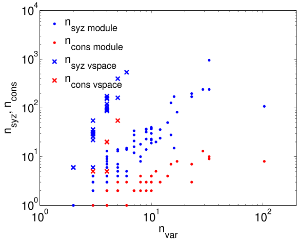
Figure 1: Computation of polynomial conservation laws arising from the generic branch of comprehensive Gröbner system for CRN models from the database Biomodels by two methods: from the generators of the syzygy module and from the basis of $\mathbb{Q}-$vector space of syzygies. $n_{var}$ is the number of variables and ODEs in the CRN model. The number of syzygies and polynomial conservation laws increases with the number of variables. When the computation of the $\mathbb{Q}-$vector space basis succeeds, the number of computed polynomial conservation laws is sensitively larger.

Availability

ODEbase is available at https://www.odebase.org/. The Singular libraries polconslaw.lib and genpolconslaw.lib are available at Zenodo under the record https://zenodo.org/record/7474523 and through Github at the following url https://github.com/oradules/polynomial_conservation_laws.

APPENDIX: Polynomial conservation laws of polynomial CRNs in the Biomodels database

Biomodels [15] is a comprehensive database of CRN models. The models of this database were mapped onto ODEbase, a canonical source of symbolic computation input [48]. We have used ODEbase for making experiments using our implementations and for testing the scalability of our computational methods for polynomial conservation laws. All of the computations were carried on a single core of an Intel i5-9400, 2.9 GHz processor, using Ubuntu 20.04 in 64-bit mode.

We have run the implementation of Algorithm 7 in two different ways:

1. First we considered only the generating set of the module of syzygies of the steady state ideals. This means not considering lines 8 and 9 of the algorithm. As explained earlier, this leads to computing some $Q[\boldsymbol{x}]$-linearly independent conservation laws, but not all possible $Q-$linearly independent conservation laws. Table LABEL:tab:table1 shows the result of the computations only for the generic branch of a comprehensive Gröbner system (as in Remark 56) and Table LABEL:tab:table2 shows the result of the computations for all branches of a comprehensive Gröbner basis. The running time for each biomodel was at most one hour.

2. Secondly, we did a full implementation of our algorithm, in order to compute a basis for the $Q$-vector space of conservation laws up to degree 4 for the generic branch of a comprehensive Gröbner basis, and up to degree 5 for all branches of a comprehensive Gröbner basis. The results can be found in Tables LABEL:tab:new-table1 and LABEL:tab:new-table2, consecutively. The running time for each biomodel was at most four hours.

Below is an interpretation of the four tables produced out of our experiments.

• Table LABEL:tab:table1 shows the result of computations of the generic branch, performed using our Singular library genpolconslaw.lib, only computing the basis for the syzygy module and not considering the vector space of syzygies up to a given degree. This results in computing some conservation laws that correspond to the conservative elements of the syzygy module basis. The computations either finished within a few seconds or did not finish after one hour. This is due to the EXPSPACE complexity of the syzygy computations (which is the same as Gröbner bases basis computation complexity). Another interesting observation concerning Table LABEL:tab:table1 is the large proportion of irrotational syzygies. For example, for Biomodel 270, there are 956 syzygies (computed just within a second), out of which only 10 syzygies are irrotational. Furthermore, with this method we only found linear unconditional conservation laws in the generic branch. We will see below that this is because the computed generators of the syzygy module correspond to linear conservation laws, which does not exclude the existence of other polynomial conservation laws.

• Table LABEL:tab:table2 shows the result of parametric polynomial conservation law computations using our Singular library polconslaw.lib. As explained in Section 6.2, parametric polynomial conservation laws result from non-generic branches. Interestingly, most of the parametric conservation laws that are computed within one hour from the non-generic branches are polynomial. Again, we must clarify that we only considered a basis of the syzygy module, but not a basis for the $Q$-vector space of syzygies up to a given degree. This results in computing only those conservation laws that arise from the syzygy module basis elements.

  We must emphasise that in Table LABEL:tab:table2, the parametric conservation laws were computed using reduced Gröbner bases, which may lead to removing some linear conservation laws in the generic branch. For instance, Biomodel 6 has two syzygies in the generic branch, and one of them is conservative, which leads to a linear conservation law ($x_{1}=const.$, resulting from $\frac{dx_{1}}{dt}=0$ and the syzygy $(1,0,0,0)$). In fact, this conservation law is not parametric, and therefore the reduction has no effect on the final result. Our calculation in Table LABEL:tab:table1 of unconditional conservation laws does not employ reduction and detects the linear conservation law $x_{1}=const.$ of the Biomodel 6.

  As expected, computing conservation laws in the generic branch is much faster than computing parametric conservation laws. Most of the computations in the generic branch are finished within one hour, but that is not the case for parametric polynomial conservation law computations. This is because when the number of branches of CGS is high, computing syzygies for all of those branches can be expensive.

• Table LABEL:tab:new-table1 shows the result of computing a basis for the $Q$-vector space of conservation laws up to degree 5 in the generic branch.

• Table LABEL:tab:new-table2 presents the result of computing a $Q$-vector space basis for syzygies up to degree 4, in each branch of a comprehensive Gröbner system. Unlike Table LABEL:tab:table2, we do not compute the reduced Gröbner basis for each branch, but rather we specialise the generators of the input steady state ideal via the conditions describing the corresponding algebraic set. This allows us to recover those parametric conservation laws that were lost during the computations in Table LABEL:tab:table2.

In comparison with computing just a basis for the syzygy module in Tables LABEL:tab:table1 and LABEL:tab:table2, computing a basis for the $Q$-vector space of syzygies up to a given degree in Tables LABEL:tab:new-table1 and LABEL:tab:new-table2 requires extra computations in lines 8 and 9 of Algorithm 7. The extra computations have exponential complexity in the number of variables and the degree bound, and therefore, may need considerably longer time for computations. This can be seen from those biomodels in Tables LABEL:tab:new-table1 and LABEL:tab:new-table2 for which the computations did not finish in four hours, while in Tables LABEL:tab:table1 and LABEL:tab:table2 the computations finished in one hour. However, theoretically, the dominant complexity factor will be the syzygy computation, which is EXPSPACE-complete, rather than the exponential factor.

As expected, when the computations finished in four hours, Tables LABEL:tab:new-table1 and LABEL:tab:new-table2 contain more polynomial conservation laws than Tables LABEL:tab:table1 and LABEL:tab:table2. In order to obtain a polynomial conservation law quickly, we recommend using syzygy modules, while for computing a basis for the $Q$-vector space of conservation laws, we recommend using the $Q$-vector space of conservative syzygies.

We note that our implemented libraries are prototype implementations of our algorithm and there is a lot of room for improvement in terms of speed and memory. For instance, one can ask the algorithm to first compute the conservative syzygies obtained from a basis of the syzygy module and then continue with computing the $Q$-vector space of conservative syzygies. Also, our implementation repeats the construction of a $Q$-vector space of syzygies up to the given degree. An improvement would be to compute such a basis once and reuse it.

Our experiments also show that all the polynomial conservation laws computed in Table LABEL:tab:new-table1 are algebraically dependent on the linear conservation laws. Indeed, $r$ independent linear conservation laws generate the linearly independent polynomial conservation laws $\phi_{1}^{n_{1}}\phi_{2}^{n_{2}}\ldots\phi_{r}^{n_{r}}$ of degree at most $d$, where $n_{1},\ldots,n_{r}$ satisfy

$$1\leq n_{1}+n_{2}+\ldots+n_{r}\leq d,n_{i}\in\mathbb{Z}_{\geq 0},1\leq i\leq r.$$ (10)

The inequalities (10) have $\binom{r+d}{d}-1$ distinct solutions. It follows that $r$ linearly independent linear conservation laws generate $\binom{r+d}{d}-1$ linearly independent polynomial conservation laws.

There are $5,20,55$ such generated polynomial conservation laws for $d=5$ and $r=1,2,3$ linear conservation laws, respectively. Comparing these numbers with the dimension of the linear space of polynomial conservation laws, given in Tables LABEL:tab:new-table1, we realize that all the conservation laws in this table are generated by linear conservation laws.

Interestingly, some non-generic branches computed in Table LABEL:tab:new-table2 have more polynomial conservation laws than those generated by the linear conservation laws, meaning that some polynomial conservation laws are algebraically independent of the linear ones. Indeed, $4,14,34,69,125,209$ conservation laws are generated by linear conservation laws for $d=4$ and $r=1,2,3,4,5,6$, respectively. Whenever we find larger numbers of conservation laws, some polynomial conservation laws are independent of the linear ones. The rows colored in gray in Table LABEL:tab:new-table2 contain polynomial conservation laws, algebraically independent of the linear ones.

Similarly, Examples 57, 58 of the main text show that polynomial conservation laws are generated by lowest degree (not necessarily linear) conservation laws. This suggests that the $\mathbb{Q}$-algebra of polynomial conservation laws is finitely generated and that the generators include curl-zero elements of a minimal basis of the syzygy module. Furthermore, the generators other than those coming from a basis of the syzygy module are rare. This subject will be further developed elsewhere.

Table 3: Conservation laws of CRNs of the database Biomodels resulting from the syzygy module basis in the generic branch of comprehensive Gröbner system. The columns represent the biomodel number, running time in seconds, the number of the generators of the syzygy module of the corresponding steady state ideal, the number of conservation laws obtained from those syzygies (equivalently, the number of irrotational syzygies in the module basis), the number of linear conservation laws, and finally the number of polynomial conservation laws for the biomodel, respectively. Blank rows show that the computations did not finish in 3600 seconds. The major part of the computation time in the algorithm is spent on computing syzygies, and for those CRNs that the computations did not finish in 3600 seconds, in fact the syzygy computation did not finish in that time period (on a single core of an Intel i5-9400, 2.9 GHz processor). $n$ and $r$ are the numbers of variables and parameters of the models, respectively.

Bio	n	r	running	# syzygy	# cons.	# lin.	# pol.
Model			time	mod. basis	laws	cons. laws	cons. laws
2	13	37	3601
6	4	7	1	2	1	1	0
28	16	31	3601
30	18	36	3601
38	17	29	6	82	8	8	0
40	5	9	1	6	2	2	0
46	16	22	3601
69	10	25	1	38	4	4	0
72	7	11	1	12	2	2	0
80	10	17	1	22	4	4	0
82	10	17	1	23	4	4	0
85	17	42	3601
86	17	56	3601
92	4	7	1	3	2	2	0
99	7	16	1	34	0	0	0
102	13	42	3601
103	17	50	3601
108	9	19	3601
150	4	5	1	3	2	2	0
156	3	8	1	3	0	0	0
159	3	8	1	3	0	0	0
198	12	20	1	24	3	3	0
199	15	18	1	28	7	7	0
200	22	54	3601
205	194	351	3603
243	23	19	1	197	3	3	0
252	4	10	1	7	0	0	0
257	11	23	3601
270	33	49	1	956	10	10	0
282	6	8	1	5	3	3	0
283	4	5	1	3	2	2	0
292	6	8	1	4	1	1	0
314	12	15	1	36	3	3	0
315	20	52	3601
335	34	54	3601
357	9	15	5	23	2	2	0
359	9	19	1	37	3	3	0
360	9	19	1	32	3	3	0
361	8	13	1	18	3	3	0
362	34	56	3601
363	4	6	1	4	1	1	0
364	14	24	3601
365	30	15	3601
405	8	7	1	8	2	2	0
430	27	52	3601
431	27	52	3601
447	13	24	3601
475	23	34	1	170	7	7	0
483	8	13	1	10	4	4	0
530	10	18	3	30	3	3	0
539	6	13	1	14	1	1	0
552	3	5	1	1	0	0	0
553	3	5	1	1	0	0	0
609	5	12	1	7	0	0	0
614	1	4	1	0	0	0	0
629	5	8	1	4	3	3	0
647	11	17	1	20	5	5	0
651	29	48	1	240	13	13	0
667	103	91	4	108	8	8	0
676	14	25	1	50	4	4	0
679	4	12	1	3	0	0	0
680	4	12	1	3	0	0	0
687	15	17	1	127	0	0	0
688	16	21	194	171	0	0	0
707	5	11	1	13	0	0	0
710	7	18	1	28	0	0	0
742	2	7	1	1	0	0	0
745	5	14	3601
747	33	54	1	240	9	9	0
748	4	9	1	10	0	0	0
755	9	11	1	14	3	3	0
758	2	5	1	1	0	0	0
780	4	16	1	9	0	0	0
781	3	11	1	4	0	0	0
782	2	7	1	1	0	0	0
783	3	9	1	4	0	0	0
793	2	5	1	1	0	0	0
795	2	7	1	1	0	0	0
815	2	7	1	1	0	0	0
827	10	18	1	37	3	3	0
854	4	11	1	4	1	1	0
868	5	10	1	5	2	2	0
870	7	17	1	16	2	2	0
875	4	9	1	6	0	0	0
880	4	15	1	10	0	0	0
882	3	6	1	2	0	0	0
886	5	19	3601
887	4	11	1	8	0	0	0
894	3	9	1	3	0	0	0
905	5	16	1	14	0	0	0
906	3	10	1	3	0	0	0
916	5	7	1	5	2	2	0
922	3	10	1	3	0	0	0
932	4	8	1	6	0	0	0
934	16	24	1	15	0	0	0
940	20	43	3601
951	34	72	3601
957	4	5	1	3	2	2	0
968	10	15	1	19	4	4	0
987	9	12	1	36	0	0	0
1004	10	21	1	40	2	2	0
1021	7	11	1	12	0	0	0
1024	2	5	1	1	0	0	0
1031	3	5	1	3	0	0	0
1035	4	12	3	13	0	0	0
1037	2	7	1	1	0	0	0
1038	3	11	1	4	0	0	0
1045	3	3	1	2	1	1	0
1053	6	7	1	15	0	0	0
1054	7	12	1	21	2	2	0

Table 4: Parametric conservation laws of CRNs of the database Biomodels resulting from computations only on a basis of the syzygy module in each branch, using our Singular library polconslaw.lib. The columns represent Biomodel number, the running time in seconds, number of branches of the corresponding comprehensive Gröbner system computed within the running time (3600 seconds on a single core of an Intel i5-9400, 2.9 GHz processor), number of the branch, the total number of conservation laws computed from the syzygy module basis elements in the branch, number of linear conservation laws computed, and finally, the number of polynomial conservation laws computed in the branch. Rows whose running time was above 3600 seconds and did not finish computing conservation laws within that branch, have blank entries under the columns of number of syzygies, and (linear/polynomial) conservation laws. Rows whose running time was below 3600 seconds but no conservation laws were found, have blank entries for the number of (linear/polynomial) conservation laws. For all the other branches, the branches leading to conservation laws are listed in the order they are found, with the corresponding number of conservation laws. To simplify the table we regrouped the branches with the same numbers of conservation laws and displayed only the numbers per subgroup. Branches are missing because they were not computed in 3600 seconds or because they do not lead to conservation laws (for instance branches 1-18 of Biomodel 40 lead to no conservation law). $n$ and $r$ are the numbers of variables and parameters of the models, respectively.

Bio-	n	r	running	# branches	# branches	# cons.	# lin.	# pol.
Model			time		per subgroup	laws	cons. laws	cons. laws
2	13	37	3601	0
6	4	7	1	7
28	16	31	3601	0
30	18	36	3601	0
38	17	29	3601	0
40	5	9	1	35	16	1	0	1
					1	2	0	2
46	16	22	3601	0
69	10	25	3601	12354	1	12	2	10
					1	19	4	15
					1	25	5	20
					1	25	5	20
72	7	11	1	74
80	10	17	3619	264	1	2	0	2
					27	4	0	4
82	10	17	3620	344	28	1	0	1
85	17	42	3606	0
86	17	56	3606	0
92	4	7	1	10
99	7	16	3620	3783	2	2	0	2
					1	8	0	8
					1	12	0	12
					1	21	0	21
					1	26	0	26
					16	32	0	32
					6	34	0	34
102	13	42	3606	0
103	17	50	3601	0
108	9	19	3601	0
150	4	5	1	10
156	3	8	1	25	16-19	2	0	2
					20-25	3	0	3
159	3	8	1	36	19-36	2	0	2
198	12	20	3481	1317	1	4	0	4
					1	8	0	8
					1	10	0	10
					1	12	0	12
					24	13	0	13
199	15	18	3610	942	1	2	0	2
					1	2	0	2
					1	7	0	7
					25	9	0	9
200	22	54	3601	0
205	194	351	3601	0
243	23	19	3606	55296	1	161	0	161
					1	300	0	300
					1	438	0	438
					1	556	0	556
					1	671	0	671
					1	795	0	795
					1	913	0	913
					1	988	0	988
					1	1040	0	1040
					1	1068	0	1068
					1	1089	0	1089
					1	1104	0	1104
					1	1114	0	1114
					1	1120	0	1120
					5	1123	0	1123
					2	1124	0	1124
					5	1125	0	1125
252	4	10	3609	175	9	1	0	1
					9	3	0	3
					3	4	0	4
					6	5	0	5
257	11	23	3601	0
270	33	49	3601	0
282	6	8	1	18
283	4	5	1	2
292	6	8	1	12
314	12	15	3608	1036	1	10	0	10
					1	17	0	17
					1	23	0	23
					1	28	0	28
					1	33	0	33
					1	37	0	37
					17	39	0	39
					5	40	0	40
315	20	52	3601	0
335	34	54	3604	0
357	9	15	3607	1953	1	1	0	1
					1	2	0	2
					1	5	0	5
					1	11	2	9
					1	17	4	13
					19	19	4	15
					3	20	4	16
359	9	19	3605	9741	1	1	0	1
					1	2	0	2
					1	6	0	6
					1	10	3	7
					1	14	4	10
					1	18	4	14
					1	21	5	16
					20	24	6	18
360	9	19	3606	7294	1	4	1	3
					1	8	1	7
					1	14	2	12
					1	19	4	15
					1	24	5	19
					1	27	6	21
					2	30	7	23
					19	31	7	24
361	8	13	3606	275	1	7	1	6
					1	11	1	10
					2	15	1	14
					21	16	1	15
					3	17	1	16
362	34	56	3601	0
363	4	6	1	15	15	2	0	2
364	14	24	3601	0
365	30	15	3601	0
405	8	7	2	23	1	1	0	1
					5	2	0	2
					7	5	0	5
					7	8	0	8
					1	10	0	10
430	27	52	3601	0
431	27	52	3601	0
447	13	24	3602	0
475	23	34	3603	0
483	8	13	3200	100	21	2	0	2
					5	3	0	3
					1	3	0	3
530	10	18	3605	33180	2	1	0	1
					1	2	0	2
					6	9	0	9
					1	12	2	10
					9	14	2	12
					7	15	2	13
539	6	13	3605	689	1	3	0	3
					24	4	0	4
					1	5	0	5
552	3	5	1	10
553	3	5	1	10
609	5	12	3606	277	24	1	0	1
614	1	4	1	5
629	5	8	1	10
647	11	17	3606	446	27	1	0	1
651	29	48	3601	0
667	103	91	3601	0
676	14	25	3601	0
679	4	12	2894	47	1	1	0	1
					28	2	0	2
680	4	12	3610	47	1	1	0	1
					28	2	0	2
687	15	17	3604	11776	26	44	0	44
688	16	21	3601	0
707	5	11	3627	341	6	1	0	1
					9	2	0	2
					8	3	0	3
					1	4	0	4
710	7	18	3605	5891	2	1	0	1
					1	3	0	3
					23	5	0	5
					1	6	0	6
742	2	7	1	35
745	5	14	3601	0
747	33	54	3601	0
748	4	9	3609	257	18	1	0	1
					10	2	0	2
755	9	11	3609	72	1	2	0	2
					1	3	0	3
					18	5	0	5
					8	6	0	6
					1	7	0	7
758	2	5	1	9
780	4	16	3606	0
781	3	11	2	132
782	2	7	1	16
783	3	9	3614	133	20	1	0	1
					1	3	0	3
					2	5	0	5
					1	6	0	6
					1	7	0	7
793	2	5	1	12
795	2	7	1	45
815	2	7	1	1
827	10	18	3607	5504	1	28	3	25
					1	36	3	33
					1	56	4	52
					1	66	5	61
					1	73	5	68
					1	75	5	70
					1	76	6	70
					1	77	7	70
					1	78	7	71
					2	79	7	72
					12	81	7	74
					4	84	8	76
					1	85	8	77
854	4	11	1	13
868	5	10	1	50
870	7	17	3609	2648	2	1	1	0
					20	3	3	0
					4	4	3	1
875	4	9	1	47	4	1	0	1
					13	4	0	4
					2	7	0	7
880	4	15	3603	0
882	3	6	1	14
886	5	19	3603	0
887	4	11	3630	211	25	1	0	1
894	3	9	1	15	6	2	0	2
					3	4	0	4
905	5	16	3606	2795	2	1	0	1
					1	2	0	2
					23	3	0	3
906	3	10	3609	135	28	1	0	1
916	5	7	17	24	1	1	0	1
					13	2	0	2
					3	4	0	4
					1	6	0	6
					8	8	0	8
922	3	10	2	46
932	4	8	7	36	20	2	0	2
934	16	24	3601	0
940	20	43	3603	0
951	34	72	3602	0
957	4	5	1	4
968	10	15	3618	356	1	2	0	2
					26	6	1	5
987	9	12	3605	521	1	14	0	14
					1	14	0	14
					1	31	0	31
					1	43	0	43
					1	51	0	51
					1	56	0	56
					1	59	0	59
					8	61	0	61
					4	63	0	63
					3	65	0	65
					1	68	0	68
					4	70	0	70
1004	10	21	3604	14905	1	7	0	7
					1	15	0	15
					1	18	0	18
					1	19	0	19
					4	22	0	22
					19	24	0	24
1021	7	11	3605	201	1	4	0	4
					1	5	0	5
					12	6	0	6
					2	8	0	8
					5	10	0	10
					6	12	0	12
1024	2	5	2	13
1031	3	5	1	16
1035	4	12	3601	0
1037	2	7	1	30	12	1	0	1
1038	3	11	3605	201	25	1	0	1
1045	3	3	1	3
1053	6	7	3106	28	1	2	0	2
					1	8	0	8
					8	11	0	11
					3	13	0	13
					1	16	0	16
					1	19	0	19
					1	22	0	22
					1	30	0	30
					1	33	0	33
					1	36	0	36
					1	44	0	44
					3	46	0	46
					1	50	0	50
					2	55	0	55
					1	59	0	59
					1	64	0	64
1054	7	12	3610	1379	1	1	0	1
					1	5	0	5
					1	9	1	8
					1	14	2	12
					1	15	3	12
					1	16	3	13
					14	17	3	14
					4	18	3	15
					5	19	3	16

Table 5: $Q$-vector space of conservation laws up to degree 5 of CRNs of the database Biomodels resulting from the $Q$-vector space of syzygies up to degree 4 in the generic branch of comprehensive Gröbner system. The columns represent the biomodel number, running time in seconds, the number of the generators of the syzygy module of the corresponding steady state ideal, dimension of the vector space of syzygies up to degree 4, the number of $Q$-linearly independent conservation laws obtained from those syzygies, (equivalently, the dimension of the $Q$-vector space of conservative syzygies up to degree 4), the number of $Q$-linearly independent linear conservation laws, and finally the number of $Q$-linealry independent polynomial conservation laws for the biomodel, respectively. Blank rows show that the computations did not finish in four hours. The major part of the computation time in the algorithm is spent on computing a basis for the syzygy module and then computing a basis for the $Q$-vector space of syzygies up to degree 4, and for those CRNs that the computations did not finish in four hours, in fact the syzygy $Q$-vector space basis computation did not finish in that time period (on a single core of an Intel i5-9400, 2.9 GHz processor). $n$ and $r$ are the numbers of variables and parameters of the models, respectively.

Bio-	n	r	running	# syzygy	dim. syzygy	# cons. laws	# lin.	# pol.
Model			time	module  basis	vector space		cons. laws	cons. laws
2	13	37	14401
28	16	31	14401
30	18	36	14401
69	10	25	14401
72	7	11	14401
80	10	17	14401
82	10	17	14401
85	17	42	14401
86	17	56	14401
92	4	7	32	3	155	20	2	18
99	7	16	14401
102	13	42	14408
103	17	50	14401
150	4	5	32	3	155	20	2	18
156	3	8	1	3	36	0	0	0
159	3	8	1	3	36	0	0	0
205	194	351	14407
243	23	19	14401
252	4	10	202	7	97	0	0	0
283	4	5	31	3	155	20	2	18
335	34	54	14401
357	9	15	14401
359	9	19	14401
360	9	19	14401
361	8	13	14401
362	34	56	14401
363	4	6	12676	4	160	5	1	4
365	30	15	14401
430	27	52	14401
431	27	52	14401
447	13	24	14401
475	23	34	14401
483	8	13	14401
539	6	13	14401
552	3	5	1	1	6	0	0	0
553	3	5	1	1	6	0	0	0
609	5	12	1756	7	162	0	0	0
614	1	4	1	0	0	0	0	0
629	5	8	517	4	399	55	3	52
647	11	17	14401
651	29	48	14401
687	15	17	14401
688	16	21	14401
707	5	11	14401
710	7	18	14401
742	2	7	1	1	6	0	0	0
745	5	14	14401
747	33	54	14401
748	4	9	722	9	87	0	0	0
755	9	11	14401
758	2	5	1	1	6	0	0	0
780	4	16	14401
781	3	11	4	4	32	0	0	0
782	2	7	1	1	6	0	0	0
783	3	9	1	4	26	0	0	0
793	2	5	1	1	6	0	0	0
795	2	7	1	1	6	0	0	0
815	2	7	1	1	6	0	0	0
827	10	18	14401
854	4	11	14401
875	4	9	281	6	121	0	0	0
880	4	15	14401
882	3	6	7	2	26	0	0	0
886	5	19	14401
887	4	11	1428	8	107	0	0	0
894	3	9	1	3	29	0	0	0
905	5	16	14401
906	3	10	22	3	22	0	0	0
916	5	7	14401
922	3	10	1	3	36	0	0	0
932	4	8	7	6	91	0	0	0
934	16	24	14401
940	20	43	14401
951	34	72	14401
957	4	5	44	3	175	20	2	18
987	9	12	14401
1004	10	21	14401
1021	7	11	14401
1024	2	5	1	1	6	0	0	0
1031	3	5	1	3	36	0	0	0
1035	4	12	14401
1037	2	7	1	1	6	0	0	0
1038	3	11	3	4	29	0	0	0
1045	3	3	2	2	55	5	1	4
1053	6	7	13567	15	540	0	0	0
1054	7	12	14405

Table 6: $Q$-vector space of parametric conservation laws of CRNs of the database Biomodels resulting from computations on $Q$-vector space of syzygies up to degree 4 in each branch of a comprehensive Gröbner basis, using our Singular library polconslaw.lib. The columns represent Biomodel number, the running time in seconds, number of branches of the corresponding comprehensive Gröbner system computed within the running time (four hours on a single core of an Intel i5-9400, 2.9 GHz processor), number of the branch, the total number of $Q$-linearly independent conservation laws computed from the $Q$-vector space of syzygies up to degree 4 in the branch, number of $Q$-linearly independent linear conservation laws computed, and finally, the number of $Q$-linearly independent polynomial conservation laws computed in the branch. Rows whose running time was above four hours and did not finish computing conservation laws within that branch, have blank entries under the columns of number of branch, number of sons. laws, and (linear/polynomial) conservation laws. For all the other branches, the branches leading to conservation laws are listed in the order they are found, with the corresponding number of conservation laws. Branches are missing because they were not computed in four hours or because they do not lead to conservation laws (for instance branches 1-2 of Biomodel 99 lead to no conservation law). To simplify the table we regrouped the branches with the same numbers of conservation laws and displayed only the numbers per subgroup. The gray rows correspond to branches containing polynomial conservation laws algebraically independent from the linear ones. $n$ and $r$ are the numbers of variables and parameters of the models, respectively.

Bio-	n	r	running	# branches	# branches	# cons.	# lin.	# pol.
Model			time		per subgroup	laws	cons. laws	cons. laws
2	13	37	14401	None
28	16	31	14401	None
30	18	36	14401	None
69	10	25	14401	12354
72	7	11	14401	74	1	14	2	12
					2	34	3	31
					2	69	4	65
					1	125	5	120
					2	209	6	203
80	10	17	14401	264
82	10	17	14401	344
85	17	42	14401	None
86	17	56	14401	None
92	4	7	87	10	6	14	2	12
					3	34	3	31
					1	69	4	65
99	7	16	14401	3783	2	4	1	3
					2	14	2	12
					2	34	3	31
					2	69	4	65
					2	125	5	120
					1	209	6	203
102	13	42	14401	None
103	17	50	14401	None
150	4	5	101	10	4	14	2	12
					5	34	3	31
					1	69	4	65
156	3	8	12	25	1	8	1	7
					9	4	1	3
					5	14	2	12
					2	34	3	31
159	3	8	14	36	13	4	1	3
					7	14	2	12
					1	34	3	31
205	194	351	14401	None
243	23	19	14401	55296
252	4	10	3372	175	11	4	1	3
					13	14	2	12
					4	34	3	31
					1	69	4	65
283	4	5	16	2	1	14	2	12
					1	34	3	31
335	34	54	14401	None
357	9	15	14401	1953
359	9	19	14401	9741
360	9	19	14401	7294
361	8	13	14401	275	1	34	3	31
					2	69	4	65
362	34	56	14401	None
363	4	6	134	15	3	4	1	3
					6	14	2	12
					5	34	3	31
					1	69	4	65
365	30	15	14401	None
430	27	52	14401	None
431	27	52	14401	None
447	13	24	14401	None
475	23	34	14401	None
483	8	13	14401	100	2	69	4	65
					1	125	5	120
539	6	13	14401	689
552	3	5	1	10	1	2	0	2
					3	4	1	3
					1	14	2	12
553	3	5	1	10	1	2	0	2
					3	4	1	3
					1	14	2	12
609	5	12	5611	277	6	4	1	3
					8	14	2	12
					9	34	3	31
					4	69	4	65
					1	125	5	120
614	1	4	1	5	2	4	1	3
629	5	8	872	10	5	34	3	31
					4	69	4	65
					1	125	5	120
647	11	17	14401	446
651	29	48	14401	None
687	15	17	14406	11775
688	16	21	14401	None
707	5	11	14401	341
710	7	18	14401	5891	2	4	1	3
					2	14	2	12
					3	34	3	31
					1	69	4	65
					2	125	5	120
742	2	7	1	35	7	4	1	3
					1	14	2	12
745	5	14	14401	None
747	33	54	14417	None
748	4	9	5471	257	14	4	1	3
					1	8	1	7
					9	14	2	12
					1	21	2	19
					3	34	3	31
755	9	11	14401	72	1	34	3	31
					1	69	4	65
758	2	5	1	9	1	2	0	2
					3	4	1	3
					1	14	2	12
780	4	16	14401	None
781	3	11	4031	132	16	4	1	3
					9	14	2	12
					2	34	3	31
782	2	7	1	16	1	4	1	3
					1	14	2	12
783	3	9	9903	133	25	4	1	3
					3	14	2	12
793	2	5	1	12	3	4	1	3
					1	14	2	12
795	2	7	1	45	5	4	1	3
					1	14	2	12
815	2	7	1	1
827	10	18	14401	5504	1	34	3	31
854	4	11	2444	13	8	4	1	3
					4	14	2	12
					1	69	4	65
875	4	9	217	47	7	4	1	3
					9	14	2	12
					2	21	2	19
					5	34	3	31
					1	69	4	65
880	4	15	14401	None
882	3	6	8	14	2	4	1	3
					4	14	2	12
					1	34	3	31
886	5	19	14401	None
887	4	11	3209	211	15	4	1	3
					1	7	1	6
					1	8	1	7
					8	14	2	12
					1	21	2	19
					1	34	3	31
					1	69	4	65
894	3	9	2	15
905	5	16	14437	2795	2	4	1	3
					3	14	2	12
					16	34	3	31
					6	69	4	65
					1	125	5	120
906	3	10	6456	135	20	4	1	3
					7	14	2	12
					1	34	3	31
916	5	7	14401	24
922	3	10	14401	46	2	4	1	3
932	4	8	9805	36	1	8	1	7
					10	4	1	3
					8	14	2	12
					6	34	3	31
					2	69	4	65
934	16	24	14401	None
940	20	43	14401	None
951	34	72	14414	None
957	4	5	43	4	2	14	2	12
					1	34	3	31
					1	69	4	65
987	9	12	14401	521
1004	10	21	14401	14905
1021	7	11	14408	201	11	4	1	3
					2	14	2	12
					5	34	3	31
					2	45	3	42
					8	69	4	65
					4	125	5	120
					1	209	6	203
1024	2	5	1	13	1	4	1	3
					1	14	2	12
1031	3	5	4	16	6	4	1	3
					2	14	2	12
1035	4	12	14406	None
1037	2	7	1	30	7	4	1	3
					1	14	2	12
1038	3	11	6537	201	19	4	1	3
					8	14	2	12
					1	34	3	31
1045	3	3	4	3	3	4	1	3
1053	6	7	14401	28	5	4	1	3
					1	21	2	19
					1	17	2	15
					1	34	3	31
					1	38	3	35
					3	69	4	65
					1	125	5	120
					2	209	6	203
1054	7	12	14401	1379

References

- [1] E. Ábrahám, J. Abbott, B. Becker, A. M. Bigatti, M. Brain, B. Buchberger, A. Cimatti, J. H. Davenport, M. England, P. Fontaine, S. Forrest, A. Griggio, D. Kroening, W. M. Seiler, and T. Sturm, : Satisfiability checking meets symbolic computation, in Proc. CICM 2016, M. Kohlhase, M. Johansson, B. Miller, L. de Moura, and F. Tompa, eds., vol. 9791 of LNCS, Springer, 2016, pp. 28–43.
- [2] R. Aris and R. Mah, Independence of chemical reactions, Industrial & Engineering Chemistry Fundamentals, 2 (1963), pp. 90–94.
- [3] V. Arnold, Mathematical methods of classical mechanics, Ann Arbor, 1001 (1978), p. 48109.
- [4] V. I. Arnold, Ordinary differential equations, Springer Textbook, Springer-Verlag, Berlin, russian ed., 1992.
- [5] P. Auger, R. B. de La Parra, J.-C. Poggiale, E. Sánchez, and L. Sanz, Aggregation methods in dynamical systems and applications in population and community dynamics, Physics of Life Reviews, 5 (2008), pp. 79–105.
- [6] C. Ballarin and M. Kauers, Solving parametric linear systems: An experiment with constraint algebraic programming, ACM SIGSAM Bulletin, 38 (2004).
- [7] C. Barrett, P. Fontaine, and C. Tinelli, The SMT-LIB standard: Version 2.6, tech. report, Department of Computer Science, The University of Iowa, 2017.
- [8] T. Becker, V. Weispfenning, and H. Kredel, Gröbner Bases, a Computational Approach to Commutative Algebra, vol. 141 of Graduate Texts in Mathematics, Springer, 1993.
- [9] C. Berkesch and F.-O. Schreyer, Syzygies, finite length modules, and random curves, Commutative algebra and noncommutative algebraic geometry, 1 (2015), pp. 25–52.
- [10] N. K. Bose, Gröbner Bases: An Algorithmic Method in Polynomial Ideal Theory, Springer Netherlands, Dordrecht, 1995, pp. 89–127, https://doi.org/10.1007/978-94-017-0275-1_4.
- [11] F. Boulier, M. Lefranc, F. Lemaire, and P.-E. Morant, Model reduction of chemical reaction systems using elimination, Mathematics in Computer Science, 5 (2011), pp. 289–301.
- [12] C. W. Brown, QEPCAD B: A program for computing with semi-algebraic sets using CADs, ACM SIGSAM Bulletin, 37 (2003), pp. 97–108, https://doi.org/10.1145/968708.968710.
- [13] C. W. Brown and C. Gross, Efficient preprocessing methods for quantifier elimination, in Computer Algebra in Scientific Computing: 9th International Workshop, CASC 2006, Chisinau, Moldova, September 11–15, 2006, V. G. Ganzha, E. W. Mayr, and E. V. Vorozhtsov, eds., vol. 4194 of Lecture Notes in Computer Science, Springer, 2006, pp. 89–100.
- [14] B. Buchberger, Ein Algorithmus zum Auffinden der Basiselemente des Restklassenringes nach einem nulldimensionalen Polynomideal, doctoral dissertation, Mathematical Institute, University of Innsbruck, Innsbruck, Austria, 1965.
- [15] V. Chelliah, N. Juty, I. Ajmera, R. Ali, M. Dumousseau, M. Glont, M. Hucka, G. Jalowicki, S. Keating, V. Knight-Schrijver, A. Lloret-Villas, K. Nath Natarajan, J.-B. Pettit, N. Rodriguez, M. Schubert, S. M. Wimalaratne, Y. Zhao, H. Hermjakob, N. Le Novère, and C. Laibe, BioModels: Ten-year anniversary, Nucl. Acids Res., 43 (2015), p. D542–D548, https://doi.org/10.1093/nar/gku1181.
- [16] G. Chèze, Computation of darboux polynomials and rational first integrals with bounded degree in polynomial time, Journal of Complexity, 27 (2011), pp. 246–262.
- [17] D. A. Cox, J. Little, and D. O’shea, Using algebraic geometry, vol. 185, Springer Science & Business Media, 2006.
- [18] D. A. Cox, J. B. Little, and D. O’Shea, Ideals, Varieties, and Algorithms, UTM, Springer, New York, fourth ed., 2015.
- [19] M. D. Darmian, A. Hashemi, and A. Montes, Erratum to ”a new algorithm for discussing Gröbner bases with parameters” [J. symbolic comput. 33(1-2) (2002) 183-208], J. Symb. Comput., 46 (2011), pp. 1187–1188, https://doi.org/10.1016/j.jsc.2011.05.002.
- [20] W. Decker, G.-M. Greuel, G. Pfister, and H. Schönemann, Singular 4-2-0 — A computer algebra system for polynomial computations. http://www.singular.uni-kl.de, 2020.
- [21] A. Desoeuvres, A. Iosif, O. Radulescu, H. Rahkooy, M. Seiß, and T. Sturm, Reduction of chemical reaction networks with approximate conservation laws, SIAM Journal on Applied Dynamical Systems, in press, (2023).
- [22] A. Dolzmann and T. Sturm, Redlog: Computer algebra meets computer logic, ACM SIGSAM Bulletin, 31 (1997), pp. 2–9.
- [23] A. Dolzmann and T. Sturm, Redlog: Computer algebra meets computer logic, ACM SIGSAM Bulletin, 31 (1997), pp. 2–9, https://doi.org/10.1145/261320.261324.
- [24] A. Dolzmann and T. Sturm, Simplification of quantifier-free formulae over ordered fields, J. Symb. Comput., 24 (1997), pp. 209–231.
- [25] A. Dolzmann, T. Sturm, and V. Weispfenning, Real quantifier elimination in practice, in Algorithmic Algebra and Number Theory, B. H. Matzat, G.-M. Greuel, and G. Hiss, eds., Springer, 1998, pp. 221–247, https://doi.org/10.1007/978-3-642-59932-3_11.
- [26] D. Eisenbud, The geometry of syzygies: A second course in commutative algebra and algebraic geometry, vol. 229, Springer, 2005.
- [27] M. Feinberg, Foundations of Chemical Reaction Network Theory, vol. 202 of Applied Mathematical Sciences, Springer, 2019, https://doi.org/10.1007/978-3-030-03858-8.
- [28] M. Feinberg and F. J. Horn, Dynamics of open chemical systems and the algebraic structure of the underlying reaction network, Chemical Engineering Science, 29 (1974), pp. 775–787.
- [29] E. Feliu and C. Wiuf, Preclusion of switch behavior in networks with mass-action kinetics, Applied Mathematics and Computation, 219 (2012), pp. 1449–1467.
- [30] N. Fenichel, Geometric singular perturbation theory for ordinary differential equations, Journal of differential equations, 31 (1979), pp. 53–98.
- [31] S. Gao, F. V. IV, and M. Wang, A new framework for computing Gröbner bases, Math. Comput., 85 (2016), pp. 449–465, https://doi.org/10.1090/mcom/2969.
- [32] A. Goeke, S. Walcher, and E. Zerz, Classical quasi-steady state reduction—a mathematical characterization, Physica D: Nonlinear Phenomena, 345 (2017), pp. 11–26, https://doi.org/10.1016/j.physd.2016.12.002.
- [33] L. Goldman, Integrals of multinomial systems of ordinary differential equations, Journal of pure and applied algebra, 45 (1987), pp. 225–240.
- [34] A. N. Gorban, O. Radulescu, and A. Y. Zinovyev, Asymptotology of chemical reaction networks, Chemical Engineering Science, 65 (2010), pp. 2310–2324.
- [35] A. Goriely, Integrability and nonintegrability of dynamical systems, vol. 19, World Scientific, 2001.
- [36] A. Hashemi, M. D. Darmian, and M. Barkhordar, Gröbner systems conversion, Math. Comput. Sci., 11 (2017), pp. 61–77, https://doi.org/10.1007/s11786-017-0295-3.
- [37] M. Hauke, Signature Gröbner bases A comprehensive survey and a new algorithmic approach, master thesis, Graz University of Technology, Graz, Austria, 2020.
- [38] A. C. Hearn, Reduce: A user-oriented interactive system for algebraic simplification, in Proc. Symposium on Interactive Systems for Experimental Applied Mathematics, ACM, 1967, https://doi.org/10.1145/2402536.2402544.
- [39] A. C. Hearn, Reduce: The first forty years, in Algorithmic Algebra and Logic: Proceedings of the A3L 2005, BOD, Norderstedt, Germany, 2005, pp. 19–24.
- [40] D. kapur, An approach for solving systems of parametric polynomial equations, Principles and Practice of Constraint Programming, (1995), p. 217–224.
- [41] D. Kapur, Comprehensive Gröbner basis theory for a parametric polynomial ideal and the associated completion algorithm, J. Syst. Sci. Complex., 30 (2017), pp. 196–233, https://doi.org/10.1007/s11424-017-6337-8.
- [42] D. Kapur, Y. Sun, and D. Wang, An efficient method for computing comprehensive Gröbner bases, J. Symb. Comput., 52 (2013), pp. 124–142, https://doi.org/10.1016/j.jsc.2012.05.015.
- [43] M. Košta, New Concepts for Real Quantifier Elimination by Virtual Substitution, doctoral dissertation, Saarland University, Germany, Dec. 2016, https://doi.org/10.22028/D291-26679.
- [44] M. Kreuzer and L. Robbiano, Computational Commutative Algebra 1, Springer Publishing Company, Incorporated, 2008.
- [45] N. Kruff, C. Lüders, O. Radulescu, T. Sturm, and S. Walcher, Algorithmic reduction of biological networks with multiple time scales, Mathematics in Computer Science, in press, (2020), https://arxiv.org/abs/2010.10129.
- [46] A. M. Lozano, The Gröbner Cover, vol. 27 of Algorithms and Computation in Mathematics, Springer, 2018, https://doi.org/10.1007/978-3-030-03904-2.
- [47] D. Lu, Y. Sun, and D. Wang, A survey on algorithms for computing comprehensive Gröbner systems and comprehensive Gröbner bases, J. Syst. Sci. Complex., 32 (2019), pp. 234–255, https://doi.org/10.1007/s11424-019-8357-z.
- [48] C. Lüders, T. Sturm, and O. Radulescu, Odebase: a repository of ode systems for systems biology, Bioinformatics Advances, 2 (2022), p. vbac027.
- [49] C. Lüders, T. Sturm, and O. Radulescu, ODEbase: A repository of ODE systems for systems biology, CoRR, abs/2201.08980 (2022), http://arxiv.org/abs/2201.08980, https://arxiv.org/abs/2201.08980.
- [50] A. Mahdi, A. Ferragut, C. Valls, and C. Wiuf, Conservation laws in biochemical reaction networks, SIAM Journal on Applied Dynamical Systems, 16 (2017), pp. 2213–2232.
- [51] Y.-K. Man, Computing closed form solutions of first order odes using the prelle-singer procedure, Journal of Symbolic Computation, 16 (1993), pp. 423–443.
- [52] L. Michaelis, M. L. Menten, et al., Die kinetik der invertinwirkung, Biochem. z, 49 (1913), p. 352.
- [53] A. Montes, A new algorithm for discussing Gröbner bases with parameters, J. Symb. Comput., 33 (2002), pp. 183–208, https://doi.org/10.1006/jsco.2001.0504.
- [54] K. Nabeshima, Generic Gröbner basis of a parametric ideal and its application to a comprehensive Gröbner system. Applications of Computer Algebra Conference, https://www.rs.tus.ac.jp/nabeshima/ACA2022/2022aca/nabeshima22.pdf, 2022.
- [55] R. Nieuwenhuis, A. Oliveras, and C. Tinelli, Solving SAT and SAT modulo theories: From an abstract Davis–Putnam–Logemann–Loveland procedure to DPLL(T), J. ACM, 53 (2006), pp. 937–977, https://doi.org/10.1145/1217856.1217859.
- [56] M. J. Prelle and M. F. Singer, Elementary first integrals of differential equations, Transactions of the American Mathematical Society, 279 (1983), pp. 215–229.
- [57] O. Radulescu, A. N. Gorban, A. Zinovyev, and V. Noel, Reduction of dynamical biochemical reactions networks in computational biology, Frontiers in genetics, 3 (2012), p. 131.
- [58] K. R. Schneider and T. Wilhelm, Model reduction by extended quasi-steady-state approximation, Journal of mathematical biology, 40 (2000), pp. 443–450.
- [59] F. O. Schreyer, A standard basis approach to syzygies of canonical curves., Journal für die reine und angewandte Mathematik, 421 (1991), pp. 83–124.
- [60] S. Schuster and T. Höfer, Determining all extreme semi-positive conservation relations in chemical reaction systems: a test criterion for conservativity, Journal of the Chemical Society, Faraday Transactions, 87 (1991), pp. 2561–2566.
- [61] A. Seidl, Cylindrical Decomposition Under Application-Oriented Paradigms, doctoral dissertation, University of Passau, Germany, Mar. 2006.
- [62] A. M. Seidl and T. Sturm, Boolean quantification in a first-order context, in Computer Algebra in Scientific Computing. Proceedings of the CASC 2003, V. G. Ganzha, E. W. Mayr, and E. V. Vorozhtsov, eds., Institut für Informatik, Technische Universität München, München, Germany, 2003, pp. 329–345.
- [63] W. Y. Sit, An algorithm for solving parametric linear systems, Journal of Symbolic Computation, 13 (1992), pp. 353–394, https://doi.org/https://doi.org/10.1016/S0747-7171(08)80104-6.
- [64] A. Sogokon, S. Mitsch, Y. K. Tan, K. Cordwell, and A. Platzer, Pegasus: Sound continuous invariant generation, Formal Methods in System Design, 58 (2021), pp. 5–41.
- [65] S. Soliman, Invariants and other structural properties of biochemical models as a constraint satisfaction problem, Algorithms for Molecular Biology, 7 (2012), pp. 1–9.
- [66] M. Spivak, Calculus on manifolds: a modern approach to classical theorems of advanced calculus, CRC press, 2018.
- [67] T. Sturm, Redlog online resources for applied quantifier elimination, Acta Acad. Ab., 67 (2007), pp. 177–191.
- [68] T. Sturm, A survey of some methods for real quantifier elimination, decision, and satisfiability and their applications, Math. Comput. Sci., 11 (2017), pp. 483–502, https://doi.org/10.1007/s11786-017-0319-z.
- [69] T. Sturm, Thirty years of virtual substitution, in Proc. ISSAC 2018, ACM, 2018, pp. 11–16.
- [70] A. Suzuki and Y. Sato, An alternative approach to comprehensive Gröbner bases, J. Symb. Comput., 36 (2003), pp. 649–667, https://doi.org/10.1016/S0747-7171(03)00098-1.
- [71] A. N. Tikhonov, Systems of differential equations containing small parameters in the derivatives, Mat. Sb. (N. S.), 73 (1952), pp. 575–586.
- [72] F. Volny, New Algorithms for Computing Groebner Bases, doctoral dissertation, Clemson University, Clemson, USA, 2011.
- [73] J. Wei and C. D. Prater, The structure and analysis of complex reaction systems, in Advances in Catalysis, vol. 13, Elsevier, 1962, pp. 203–392.
- [74] V. Weispfenning, Comprehensive Gröbner bases, J. Symb. Comput., 14 (1992), pp. 1–30, https://doi.org/10.1016/0747-7171(92)90023-W.
- [75] X. Zhang, Integrability of dynamical systems: algebra and analysis, vol. 47, Springer, 2017.