Depth-First Search performance in a random digraph with geometric outdegree distribution

Abstract.

We present an analysis of the depth-first search algorithm in a random digraph model with independent outdegrees having a geometric distribution.

The results include asymptotic results for the depth profile of vertices, the height (maximum depth) and average depth, the number of trees in the forest, the size of the largest and second-largest trees, and the numbers of arcs of different types in the depth-first jungle. Most results are first order. For the height we show an asymptotic normal distribution.

This analysis proposed by Donald Knuth in his next to appear volume of The Art of Computer Programming gives interesting insight in one of the most elegant and efficient algorithm for graph analysis due to Tarjan.

1. Introduction

The motivation of this paper is a new section in Donald Knuth’s The Art of Computer Programming [13], which is dedicated to Depth-First Search (DFS) in a digraph. Briefly, the DFS starts with an arbitrary vertex, and explores the arcs from that vertex one by one. When an arc is found leading to a vertex that has not been seen before, the DFS explores the arcs from that vertex in the same way, in a recursive fashion, before returning to the next arc from its parent. This eventually yields a tree containing all descendants of the the first vertex (which is the root of the tree). If there still are some unseen vertices, the DFS starts again with one of them and finds a new tree, and so on until all vertices are found. We refer to [13] for details as well as for historical notes. (See also S1–S2 in Section 4.) Note that the digraphs in [13] and here are multi-digraphs, where loops and multiple arcs are allowed. (Although in our random model these are few and usually not important.) The DFS algorithm generates a spanning forest (the depth-first forest) in the digraph, with all arcs in the forest directed away from the roots. Our main purpose is to study the properties of the depth-first forest, starting with a random digraph $G$; in particular we study the distribution of the depth of vertices in the depth-first forest.

The random digraph model that we consider (following Knuth [13]) has $n$ vertices and a given outdegree distribution $\mathbf{P}$, which in the main part of the present paper is a geometric distribution $\operatorname{Ge}(1-p)$ for some fixed $0<p<1$. The outdegrees (number of outgoing arcs) of the $n$ vertices are independent random numbers with this distribution. The endpoint of each arc is uniformly selected at random among the $n$ vertices, independently of all other arcs. (Therefore, an arc can loop back to the starting vertex, and multiple arcs can occur.) We consider asymptotics as $n\to\infty$ for a fixed outdegree distribution.

In the present paper, we study the case of a geometric outdegree distribution in detail; we also (in Section 3) briefly give corresponding results for the shifted geometric outdegree distribution $\operatorname{Ge}_{1}(1-p)$, and discuss the similarities and differences between the two cases. The case of a general outdegree distribution (with finite variance) will be studied in a forthecoming paper [11], where we use a somewhat different method which allows us to extend many (but not all) of the results in the present paper and obtain similar, but partly weaker, results; see also Section 4. One reason for studying the geometric case separately is that its lack-of-memory property leads to interesting features and simplifications not present for general outdegree distributions; this is seen both in [13] and in the proofs and results below. In particular, the depth process studied in Section 2 will be a Markov chain, which is the basis of our analysis.

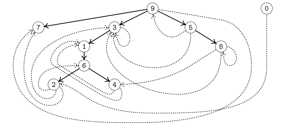
In addition to studying the depth-first forest, we give also (in Section 2.5) some results on the number of edges of different types in the depth-first jungle; this is defined in [13] as the original digraph with arcs classified by the DFS algorithm into the following five types, see Figure 1 for examples:

• loops;

• tree arcs, the arcs in the resulting depth-first forest;

• back arcs, the arcs which point to an ancestor of the current vertex in the current tree;

• forward arcs, the arcs which point to an already discovered descendant of the current vertex in the current tree;

• cross arcs, all other arcs (these point to an already discovered vertex which is neither a descendant nor an ancestor of the current vertex, and might be in another tree).

(See further the exercises in [13].)

Figure 1. Example of a depth-first forest (jungle) from [13], by courtesy of Donald Knuth. Tree arcs are solid (e.g. ⑨$\to$ ③). For example, ③$\dasharrow$ ③ is a loop, ②$\dasharrow$ ③ is a back arc, ⑨$\dasharrow$ ⑦ is a forward arc, ⑧$\dasharrow$ ④ and ⓪$\dasharrow$ ② are cross arcs.

Remark 1.1.

Some related results for DFS in an undirected Erdős–Rényi graph $G(n,\lambda/n)$ are proved by Enriquez, Faraud and Ménard [6] and Diskin and Krivelevich [5], and DFS in a random Erdős–Rényi digraph has been studied for example in the proof of [14, Theorem 3]. These models are closely related to our model with a Poisson outdegree distribution $\mathbf{P}$; they will therefore be further discussed in [11].

Remark 1.2.

We consider only the case of a fixed outdegree distribution $\mathbf{P}$. The results can be extended to distributions $\mathbf{P}_{n}$ depending on $n$, under suitable conditions. This is particularly interesting in the critical case, with expectations $\lambda_{n}\to 1$; however, this is out of the scope of the present paper.

The main results for a geometric out-degree distribution are stated and proved in Section 2. We analyze the process $d(t)$ of depths of the vertices, in the order they are found by the DFS. For a geometric outdegree distribution (but not in general), $d(t)$ is a Markov chain, and we find its first-order limit by a martingale argument; moreover, we show Gaussian fluctuations. We also find results for the numbers of different types of arcs defined above; this includes verifying some conjectures from previous versions of [13].

In Section 3 we study briefly the case of a shifted geometric outdegree distribution. The same method as in Section 2 works in this case too, but the explicit results are somewhat different. One motivation for this section is to show that some of the relations found in Section 2 for a geometric outdegree distribution do not hold for arbitrary distributions.

We end in Section 4 with some comments on the case of general outdegree distributions.

1.1. Some notation

We denote the given outdegree distribution by $\mathbf{P}$. Recall that our standing assumption is that the outdegrees of the vertices are i.i.d. (independent and identically distributed).

The mean outdegree, i.e., the expectation of $\mathbf{P}$, is denoted by $\lambda$. In analogy with branching processes, we say that the random digraph is subcritical if $\lambda<1$, critical if $\lambda=1$, and supercritical if $\lambda>1$.

As usual, w.h.p. means with high probability, i.e., with probability $1-o(1)$ as ${n\to\infty}$. We use $\overset{\mathrm{p}}{\longrightarrow}$ for convergence in probability, and $\overset{\mathrm{d}}{\longrightarrow}$ for convergence in distribution of random variables.

Moreover, let $(a_{n})$ be a sequence of positive numbers, and $X_{n}$ a sequence of random variables. We write $X_{n}=o_{\mathrm{p}}(a_{n})$ if, as ${n\to\infty}$, $X_{n}/a_{n}\overset{\mathrm{p}}{\longrightarrow}0$, i.e., if for every $\varepsilon>0$, we have $\operatorname{\mathbb{P}{}}(|X_{n}|>\varepsilon a_{n})\to 0$. Note that this is equivalent to the existence of a sequence $\varepsilon_{n}\to 0$ such that $\operatorname{\mathbb{P}{}}(|X_{n}|>\varepsilon_{n}a_{n})\to 0$, or in other words $|X_{n}|\leq\varepsilon_{n}a_{n}$ w.h.p. (This is sometimes denoted “$X_{n}=o(a_{n})$ w.h.p.”, but we will not use this notation.)

Furthermore, $X_{n}=O_{L^{2}}(a_{n})$ means $\operatorname{\mathbb{E}{}}\bigl{[}|X_{n}/a_{n}|^{2}\bigr{]}=O(1)$. Note that $X_{n}=O_{L^{2}}(a_{n})$ implies $X_{n}=o_{\mathrm{p}}(\omega_{n}a_{n})$, for any sequence $\omega_{n}\to\infty$. Note also that $X_{n}=O_{L^{2}}(a_{n})$ implies $\operatorname{\mathbb{E}{}}X_{n}=O(a_{n})$; thus error terms of this type implies immediately estimates for expectations and second moments. In particular, for the most common case below, $X_{n}=O_{L^{2}}(n^{1/2})$ is equivalent to $\operatorname{\mathbb{E}{}}X_{n}=O(n^{1/2})$ and $\operatorname{Var}X_{n}=O(n)$.

$\operatorname{Ge}(1-p)$ denotes the geometric distribution on $\{0,1,\dots\}$; thus $\eta\sim\operatorname{Ge}(1-p)$ means that $\eta$ is a random variable with $\operatorname{\mathbb{P}{}}(\eta=k)=p^{k}(1-p)$, $k\geq 0$. Similarly, $\operatorname{Ge}_{1}(1-p)$ denotes the shifted geometric distribution on $\{1,2,\dots\}$; thus $\eta\sim\operatorname{Ge}_{1}(1-p)$ means $\operatorname{\mathbb{P}{}}(\eta=k)=p^{k-1}(1-p)$, $k\geq 1$. $\operatorname{Po}(\lambda)$ denotes a Poisson distribution with mean $\lambda$.

We define $\rho_{0}(x)$, for $x\geq 0$, as the largest solution in $[0,1)$ to

$$1-\rho_{0}=e^{-x\rho_{0}}.$$ (1.1)

As is well known, $\rho_{0}(x)$ is the survival probability of a Galton–Watson process with a Poisson offspring distribution $\operatorname{Po}(x)$ with mean $x$. We have $\rho_{0}(x)=0$ for $x\leq 1$ and $0<\rho_{0}(x)<1$ for $x>1$. (See e.g. [3, Theorem I.5.1].)

For a real number $x$, we write $x^{+}:=\max\{x,0\}$. $[n]:=\{1,\dots,n\}$. All logarithms are natural. $C$ and $c$ are sometimes used for positive constants.

Remark 1.3.

We state many results with error estimates in $L^{2}$, which means estimates on the second moment; we conjecture that the results extend to higher moment and estimates in $L^{p}$ for any $p<\infty$, but we have not pursued this.

2. Depth analysis with geometric outdegree distribution

In this section we assume that the outdegree distribution is geometric $\operatorname{Ge}(1-p)$ for some fixed $0<p<1$, and thus has mean

$$\lambda:=\frac{p}{1-p}.$$ (2.1)

When doing the DFS on a random digraph of the type studied in this paper, it is natural to reveal the outdegree of a vertex as soon as we find it. (See S1–S2 in Section 4.) However, for a geometric outdegree distribution, because of its lack-of-memory property, we do not have to immediately reveal the outdegree when we find a new vertex $v$. Instead, we only check whether there is at least one outgoing arc (probability $p$), and if so, we find its endpoint and explore this endpoint if it has not already been visited; eventually, we return to $v$, and then we check whether there is another outgoing arc (again probability $p$, by the lack-of-memory property), and so on. This will yield the important Markov property in the construction in the next subsection.

In the following, by a future arc from some vertex, we mean an arc that at the current time has not yet been seen by the DFS.

2.1. Depth Markov chain

Our aim is to track the evolution of the search depth as a function of the number $t$ of discovered vertices. Let $v_{t}$ be the $t$-th vertex discovered by the DFS ($t=1,\dots,n$), and let $d(t)$ be the depth of $v_{t}$ in the resulting depth-first forest, i.e., the number of tree edges that connect the root of the current tree to $v_{t}$. The first found vertex $v_{1}$ is a root, and thus $d(1)=0$.

The quantity $d(t)$ follows a Markov chain with transitions ($1\leq t<n$):

1. $d(t+1)=d(t)+1$.
   This happens if, for some $k\geq 1$, $v_{t}$ has at least $k$ outgoing arcs, the first $k-1$ arcs lead to vertices already visited, and the $k$th arc leads to a new vertex (which then becomes $v_{t+1}$). The probability of this is

   $$\sum_{k=1}^{\infty}p^{k}\Bigl{(}\frac{t}{n}\Bigr{)}^{k-1}\Bigl{(}1-\frac{t}{n}\Bigr{)}=\frac{(1-t/n)p}{1-pt/n}.$$ (2.2)

2. $d(t+1)=d(t)$, assuming $d(t)>0$.
   This holds if all arcs from $v_{t}$ lead to already visited vertices, i.e., (i) does not happen, and furthermore, the parent of $v_{t}$ has at least one future arc leading to an unvisited vertex. These two events are independent. Moreover, by the lack-of-memory property, the number of future arcs from the parent of $v_{t}$ has also the distribution $\operatorname{Ge}(1-p)$. Hence, the probability that one of these future arcs leads to an unvisited vertex equals the probability in (2.2). The probability of (ii) is thus

   $$\Bigl{(}1-\frac{(1-t/n)p}{1-pt/n}\Bigr{)}\frac{(1-t/n)p}{1-pt/n}.$$ (2.3)

3. $d(t+1)=d(t)-\ell$, assuming $d(t)>\ell\geq 1$.
   This happens if all arcs from $v_{t}$ lead to already visited vertices, and so do all future arcs from the $\ell$ nearest ancestors of $v_{t}$, while the $(\ell+1)$th ancestor has at least one future arc leading to an unvisited vertex. The argument in (ii) generalizes and shows that this has probability

   $$\Bigl{(}1-\frac{(1-t/n)p}{1-pt/n}\Bigr{)}^{\ell+1}\frac{(1-t/n)p}{1-pt/n}.$$ (2.4)

4. $d(t+1)=d(t)-\ell$, assuming $d(t)=\ell\geq 0$.
   By the same argument as in (ii) and (iii), except that the $(\ell+1)$th ancestor does not exist and we ignore it, we obtain the probability

   $$\Bigl{(}1-\frac{(1-t/n)p}{1-pt/n}\Bigr{)}^{\ell+1}.$$ (2.5)

Note that (iv) is the case when $d(t+1)=0$ and thus $v_{t+1}$ is the root of a new tree in the depth-first forest.

We can summarize (i)–(iv) in the formula

$$d(t+1)=\bigl{(}d(t)+1-\xi_{t}\bigr{)}^{+},$$ (2.6)

where $\xi_{t}$ is a random variable, independent of the history, with the distribution

$$\operatorname{\mathbb{P}{}}(\xi_{t}=k)=(1-\pi_{t})^{k}\pi_{t},\quad k\geq 0,$$ (2.7)

where

$$\pi_{t}:=\frac{(1-t/n)p}{1-pt/n}=1-\frac{1-p}{1-pt/n}.$$ (2.8)

In other words, $\xi_{t}$ has the geometric distribution $\operatorname{Ge}(\pi_{t})$. Define

$$\widetilde{d}(t):=\sum_{i=1}^{t-1}(1-\xi_{i}),$$ (2.9)

and note that (2.9) is a sum of independent random variables. Then $d(t)$ can be recovered from the simpler process $\widetilde{d}(t)$ as follows.

Lemma 2.1.

We have

$$d(t)=\widetilde{d}(t)-\min_{1\leq j\leq t}\widetilde{d}(j),\qquad 1\leq t\leq n.$$ (2.10)

Proof.

We use induction on $t$. Evidently, (2.10) holds for $t=1$ since $d(1)=\widetilde{d}(1)=0$.

Suppose that (2.10) holds for some $t<n$. Then (2.9) yields

$$\widetilde{d}(t+1)=\widetilde{d}(t)+1-\xi_{t}=d(t)+1-\xi_{t}+\min_{1\leq j\leq t}\widetilde{d}(j).$$ (2.11)

If $d(t)+1-\xi_{t}\geq 0$, then (2.11) shows that $\widetilde{d}(t+1)\geq\min_{1\leq j\leq t}\widetilde{d}(j)$, and thus $\min_{1\leq j\leq t+1}\widetilde{d}(j)=\min_{1\leq j\leq t}\widetilde{d}(j)$; furthermore, $d(t+1)=d(t)+1-\xi_{t}$ by (2.6), and it follows that (2.10) holds for $t+1$.

On the other hand, if $d(t)+1-\xi_{t}<0$, then (2.11) shows that $\widetilde{d}(t+1)<\min_{1\leq j\leq t}\widetilde{d}(j)$, and thus $\min_{1\leq j\leq t+1}\widetilde{d}(j)=\widetilde{d}(t+1)$. In this case, $d(t+1)=0$ by (2.6), and it follows that (2.10) holds for $t+1$ in this case too. ∎

Remark 2.2.

Similar formulas have been used for other, related, problems with random graphs and trees, where trees have been coded as walks, see for example [2, Section 1.3]. Note that in our case, unlike e.g. [2], $\widetilde{d}(t)$ may have negative jumps of arbitrary size.

2.2. Main result for depth analysis

Note first that (2.8) implies that, using $\lambda=p/(1-p)$,

$$\mu_{t}:=\operatorname{\mathbb{E}{}}\xi_{t}=\frac{1-\pi_{t}}{\pi_{t}}=\frac{1-p}{p(1-t/n)}=\frac{1}{\lambda(1-t/n)}.$$ (2.12)

Hence, (2.9) implies that the expectation of $\widetilde{d}(t)$ is

$$\operatorname{\mathbb{E}{}}\bigl{[}\widetilde{d}(t)\bigr{]} =\sum_{i=1}^{t-1}(1-\operatorname{\mathbb{E}{}}\xi_{i})=\sum_{i=1}^{t-1}(1-\mu_{i})=\sum_{i=1}^{t-1}\Bigl{(}1-\frac{1}{\lambda(1-i/n)}\Bigr{)}.$$ (2.13)

Let $\theta:=t/n$. We fix a $\theta^{*}<1$ and obtain that, uniformly for $\theta\leq\theta^{*}$,

$$\operatorname{\mathbb{E}{}}\bigl{[}\widetilde{d}(t)\bigr{]}=\int_{0}^{t}\Bigl{(}1-\frac{1}{\lambda(1-x/n)}\Bigr{)}\,\mathrm{d}x+O(1)=n\widetilde{\ell}(\theta)+O(1),$$ (2.14)

where

$$\widetilde{\ell}(\theta):=\int_{0}^{\theta}\Bigl{(}1-\frac{1}{\lambda(1-x)}\Bigr{)}\,\mathrm{d}x=\theta+\lambda^{-1}\log(1-\theta).$$ (2.15)

Note that the derivative $\widetilde{\ell}^{\prime}(\theta)=1-\lambda^{-1}/(1-\theta)$ is (strictly) decreasing on $(0,1)$, i.e., $\widetilde{\ell}$ is concave. Moreover, if $\lambda>1$ (i.e., $p>\frac{1}{2}$) (the supercritical case), then $\widetilde{\ell}^{\prime}(0)>0$, and (2.15) shows that $\widetilde{\ell}(\theta)$ is positive and increasing for $\theta<\theta_{0}:=1-\lambda^{-1}=(2p-1)/p$. After the maximum at $\theta_{0}$, $\widetilde{\ell}(\theta)$ decreases and tends to $-\infty$ as $\theta\nearrow 1$. Hence, there exists a $\theta_{0}<\theta_{1}<1$ such that $\widetilde{\ell}(\theta_{1})=0$; we then have $\widetilde{\ell}(\theta)>0$ for $0<\theta<\theta_{1}$ and $\widetilde{\ell}(\theta)<0$ for $\theta>\theta_{1}$. We will see that in this case the depth-first forest w.h.p. contains a giant tree, of order and height both linear in $n$, while all other trees are small.

On the other hand, if $\lambda\leq 1$ (i.e., $p\leq\frac{1}{2}$) (the subcritical and critical cases), then $\widetilde{\ell}^{\prime}(0)\leq 0$ and $\widetilde{\ell}(\theta)$ is negative and decreasing for all $\theta\in(0,1)$. In this case, we define $\theta_{0}:=\theta_{1}:=0$ and note that the properties just stated for $\widetilde{\ell}$ still hold (rather trivially). We will see that in this case w.h.p. all trees in the depth-first forest are small.

Note that in all cases,

$$\theta_{0}:=\bigl{(}1-\lambda^{-1}\bigr{)}^{+}=\begin{cases}1-\lambda^{-1},&\lambda>1,\\ 0,&\lambda\leq 1,\end{cases}$$ (2.16)

and that $\theta_{1}$ is the largest solution in $[0,1)$ to

$$\log(1-\theta_{1})=-\lambda\theta_{1}.$$ (2.17)

Remark 2.3.

The equation (2.17) may also be written $1-\theta_{1}=\exp(-\lambda\theta_{1})$, which shows that

$$\theta_{1}=\rho_{0}(\lambda),$$ (2.18)

the survival probability of a Galton–Watson process with $\operatorname{Po}(\lambda)$ offspring distribution defined in (1.1).

We define $\widetilde{\ell}^{+}(\theta):=[\widetilde{\ell}(\theta)]^{+}$. Thus, by (2.15) and the comments above,

$$\widetilde{\ell}^{+}(\theta)=\begin{cases}\theta+\lambda^{-1}\log(1-\theta),&0\leq\theta\leq\theta_{1},\\ 0,&\theta_{1}\leq\theta\leq 1.\end{cases}$$ (2.19)

We can now state one of our main results.

Theorem 2.4.

We have

$$\max_{1\leq t\leq n}\bigl{\lvert}d(t)-n\widetilde{\ell}^{+}(t/n)\bigr{\rvert}=O_{L^{2}}(n^{1/2}).$$ (2.20)

Proof.

Since (2.9) is a sum of independent random variables, $\widetilde{d}(t)-\operatorname{\mathbb{E}{}}\widetilde{d}(t)$ ($t=1,\dots,n$) is a martingale, and Doob’s inequality [7, Theorem 10.9.4] yields, for all $T\leq n$,

$$\operatorname{\mathbb{E}{}}\bigl{[}\max_{t\leq T}|\widetilde{d}(t)-\operatorname{\mathbb{E}{}}\widetilde{d}(t)|^{2}\bigr{]}\leq 4\operatorname{\mathbb{E}{}}\bigl{[}|\widetilde{d}(T)-\operatorname{\mathbb{E}{}}\widetilde{d}(T)|^{2}\bigr{]}=4\sum_{i=1}^{T-1}\operatorname{Var}(\xi_{i}).$$ (2.21)

As above, fix $\theta^{*}<1$, and assume, as we may, that $\theta^{*}>\theta_{1}$. Let $T^{*}:=\lfloor n\theta^{*}\rfloor$, and consider first $t\leq T^{*}$. For $i<T^{*}$, we have $\operatorname{Var}\xi_{i}=O(1)$, and thus, for $T=T^{*}$, the sum in (2.21) is $O(T^{*})=O(n)$. Consequently, (2.21) yields

$$\max_{t\leq T^{*}}\bigl{\lvert}\widetilde{d}(t)-\operatorname{\mathbb{E}{}}\widetilde{d}(t)\bigr{\rvert}=O_{L^{2}}(n^{1/2}).$$ (2.22)

Hence, by (2.14),

$$M^{*}:=\max_{t\leq T^{*}}\bigl{\lvert}\widetilde{d}(t)-n\widetilde{\ell}(t/n)\bigr{\rvert}=O_{L^{2}}(n^{1/2}).$$ (2.23)

(Note that $T^{*}$ and $M^{*}$ depend on the choice of $\theta^{*}$.) For $t\leq T^{*}$, the definition of $M^{*}$ in (2.23) implies

$$\Bigl{\lvert}\min_{1\leq j\leq t}\widetilde{d}(j)-n\min_{1\leq j\leq t}\widetilde{\ell}(j/n)\Bigr{\rvert}\leq M^{*}.$$ (2.24)

Moreover, for $t/n\leq\theta_{1}$, we have $\min_{1\leq j\leq t}\widetilde{\ell}(j/n)=O(1/n)$, while for $t/n\geq\theta_{1}$, we have $\min_{1\leq j\leq t}\widetilde{\ell}(j/n)=\widetilde{\ell}(t/n)$. Hence, for all $t\leq T^{*}$,

$$\min_{1\leq j\leq t}\widetilde{\ell}(j/n)=\widetilde{\ell}(t/n)-\widetilde{\ell}^{+}(t/n)+O(1/n),$$ (2.25)

and thus, by (2.24),

$$\Bigl{\lvert}\min_{1\leq j\leq t}\widetilde{d}(j)-n\widetilde{\ell}(t/n)+n\widetilde{\ell}^{+}(t/n)\Bigr{\rvert}\leq M^{*}+O(1/n).$$ (2.26)

Finally, by (2.10), (2.23) and (2.26),

$$\bigl{\lvert}d(t)-n\widetilde{\ell}^{+}(t/n)\bigr{\rvert}\leq 2M^{*}+O(1/n).$$ (2.27)

This holds uniformly for $t\leq T^{*}$, and thus, by (2.23),

$$\max_{1\leq t\leq T^{*}}\bigl{\lvert}d(t)-n\widetilde{\ell}^{+}(t/n)\bigr{\rvert}=O_{L^{2}}(n^{1/2}).$$ (2.28)

It remains to consider $T^{*}<t\leq n$. Then the argument above does not quite work, because $\pi_{t}\searrow 0$ and thus $\operatorname{Var}\xi_{t}\nearrow\infty$ as $t\nearrow n$. We therefore modify $\xi_{t}$. We define $\widehat{\pi}_{t}:=\max\{\pi_{t},\pi_{T^{*}}\}$; thus $\widehat{\pi}_{t}=\pi_{t}$ for $t\leq T^{*}$ and $\widehat{\pi}_{t}>\pi_{t}$ for $t>T^{*}$. We may then define independent random variables $\widehat{\xi}_{t}$ such that $\widehat{\xi}_{t}\sim\operatorname{Ge}(\widehat{\pi}_{t})$ and $\widehat{\xi}_{t}\leq\xi_{t}$ for all $t<n$. (Thus, $\widehat{\xi}_{t}=\xi_{t}$ for $t\leq T^{*}$.)

In analogy with (2.9)–(2.10), we further define

$$\widehat{\widetilde{d}}(t) :=\sum_{i=1}^{t-1}\bigl{(}1-\widehat{\xi}_{i}\bigr{)},$$ (2.29)

$$\widehat{d}(t) :=\widehat{\widetilde{d}}(t)-\min_{1\leq j\leq t}\widehat{\widetilde{d}}(j)=\max_{1\leq j\leq t}\sum_{i=j}^{t-1}\bigl{(}1-\widehat{\xi}_{i}\bigr{)}.$$ (2.30)

Since $\widehat{\xi}_{i}\leq\xi_{i}$, (2.30) implies that $\widehat{d}(t)\geq d(t)$ for all $t$.

We have $\operatorname{Var}\bigl{[}\widehat{\xi}_{t}\bigr{]}=O(1)$, uniformly for all $t<n$, and thus the argument above yields

$$\max_{1\leq t\leq n}\bigl{\lvert}\widehat{d}(t)-n[\widehat{\widetilde{\ell}}(t/n)]^{+}\bigr{\rvert}=O_{L^{2}}(n^{1/2}),$$ (2.31)

where

$$\widehat{\widetilde{\ell}}(\theta):=\int_{0}^{\theta}\min\Bigl{\{}\Bigl{(}1-\frac{1}{\lambda(1-x)}\Bigr{)},\Bigl{(}1-\frac{1}{\lambda(1-\theta^{*})}\Bigr{)}\Bigr{\}}\,\mathrm{d}x.$$ (2.32)

We have $\widehat{\widetilde{\ell}}(\theta)=\widetilde{\ell}(\theta)$ for $\theta\leq\theta^{*}$, and for $\theta\geq\theta^{*}$, $\widehat{\widetilde{\ell}}(\theta)$ is negative and decreasing (since $\theta^{*}>\theta_{1}$). Hence, $[\widehat{\widetilde{\ell}}(\theta)]^{+}=\widetilde{\ell}^{+}(\theta)$ for all $0<\theta\leq 1$. In particular, $[\widehat{\widetilde{\ell}}(\theta)]^{+}=\widetilde{\ell}^{+}(\theta)=0$ for all $\theta\geq\theta^{*}$, and (2.31) implies

$$\max_{T^{*}<t\leq n}\widehat{d}(t)=O_{L^{2}}(n^{1/2}).$$ (2.33)

Recalling $0\leq d(t)\leq\widehat{d}(t)$, we thus have

$$\max_{T^{*}<t\leq n}\bigl{\lvert}d(t)-n\widetilde{\ell}^{+}(t/n)\bigr{\rvert}=\max_{T^{*}<t\leq n}d(t)\leq\max_{T^{*}<t\leq n}\widehat{d}(t)=O_{L^{2}}(n^{1/2}),$$ (2.34)

which completes the proof. ∎

Corollary 2.5.

The height $\Upsilon$ of the depth-first forest is

$$\Upsilon:=\max_{1\leq t\leq n}d(t)=\upsilon n+O_{L^{2}}(n^{1/2}),$$ (2.35)

where

$$\upsilon=\upsilon(p):=\widetilde{\ell}^{+}(\theta_{0})=\begin{cases}0,&0<\lambda\leq 1,\\ 1-\lambda^{-1}-\lambda^{-1}\log\lambda,&\lambda>1.\end{cases}$$ (2.36)

Proof.

Immediate from Theorem 2.4 and (2.15), since we have $\max_{t}\widetilde{\ell}^{+}(t/n)=\max_{\theta}\widetilde{\ell}^{+}(\theta)+O(1/n)$ and $\max_{\theta}\widetilde{\ell}^{+}(\theta)=\widetilde{\ell}^{+}(\theta_{0})=\widetilde{\ell}(\theta_{0})$. ∎

In Section 2.3 we will improve this when $\lambda>1$, and show that then the height $\Upsilon$ is asymptotically normally distributed (Theorem 2.11).

Corollary 2.6.

The average depth $\overline{d}$ in the depth-first forest is

$$\overline{d}:=\frac{1}{n}\sum_{t=1}^{n}d(t)=\alpha n+O_{L^{2}}(n^{1/2}),$$ (2.37)

where $\alpha=0$ if $\lambda\leq 1$, and, in general,

$$\alpha=\alpha(p):=\frac{1}{2}\theta_{1}^{2}-\frac{1}{\lambda}\Bigl{(}(1-\theta_{1})\log(1-\theta_{1})+\theta_{1}\Bigr{)}=\frac{\lambda-1}{\lambda}\,\theta_{1}-\frac{1}{2}\theta_{1}^{2}.$$ (2.38)

Proof.

By Theorem 2.4,

$$\frac{1}{n}\sum_{t=1}^{n}d(t)=\sum_{t=1}^{n}\widetilde{\ell}^{+}(t/n)+O_{L^{2}}\bigl{(}n^{1/2}\bigr{)}=n\alpha+O_{L^{2}}\bigl{(}n^{1/2}\bigr{)},$$ (2.39)

where

$$\alpha :=\int_{0}^{1}\widetilde{\ell}^{+}(x)\,\mathrm{d}x=\int_{0}^{\theta_{1}}\widetilde{\ell}(x)\,\mathrm{d}x=\int_{0}^{\theta_{1}}\Bigl{(}x+\lambda^{-1}\log(1-x)\Bigr{)}\,\mathrm{d}x$$

$$\phantom{:}=\frac{1}{2}\theta_{1}^{2}-\lambda^{-1}\Bigl{(}(1-\theta_{1})\log(1-\theta_{1})+\theta_{1}\Bigr{)},$$ (2.40)

which yields (2.38), using (2.17). ∎

Remark 2.7.

When $\lambda>1$, the height $\Upsilon$ and average depth $\overline{d}$ are thus linear in $n$, unlike many other types of random trees. This might imply a rather slow performance of algorithms that operate on the depth-first forest if it is built explicitly in a computer’s memory.

2.3. Asymptotic normality

In this subsection, we show that in the supercritical case $\lambda>1$, Theorem 2.4 can be improved to yield convergence of $d(t)$ (after rescaling) to a Gaussian process, at least on $[0,\theta_{1})$. As a consequence, we show that the height $\Upsilon$ is asymptotically normal.

Recall that for an interval $I\subseteq\mathbb{R}$, $D(I)$ is the space of functions $I\to\mathbb{R}$ that are right-continuous with left limits (càdlàg) equipped with the Skorohod topology. For definitions of the topology see e.g. [4], [8], [12, Appendix A.2], or [9]; for our purposes it is enough to know that convergence in $D(I)$ to a continuous limit is equivalent to uniform convergence on compact subsets of $I$. (Note that it thus matters if the endpoints are included in $I$ or not; for example, convergence in $D[0,1)$ and $D[0,1]$ mean different things.)

We define $d(0):=\widetilde{d}(0):=0$.

Lemma 2.8.

Assume $\lambda>1$. Then

$$n^{-1/2}\bigl{(}\widetilde{d}(\lfloor n\theta\rfloor)-n\widetilde{\ell}(\theta)\bigr{)}\overset{\mathrm{d}}{\longrightarrow}Z(\theta)\qquad\text{in $D[0,1)$},$$ (2.41)

where $Z(\theta)$ is a continuous Gaussian process on $[0,1)$ with mean $\operatorname{\mathbb{E}{}}Z(\theta)=0$ and covariance $\operatorname{Cov}\bigl{(}Z(x),Z(y)\bigr{)}=v\bigl{(}\min\{x,y\}\bigr{)}$, where

$$v(\theta):=\frac{(1-p)^{2}\theta}{p^{2}(1-\theta)}-\frac{1-p}{p}\log(1-\theta)=\lambda^{-2}\frac{\theta}{1-\theta}-\lambda^{-1}\log(1-\theta).$$ (2.42)

Equivalently, $Z(\theta)=B\bigl{(}v(\theta)\bigr{)}$ for a Brownian motion $B(x)$.

Proof.

Since the random variables $\xi_{t}$ are independent, (2.9) and (2.7)–(2.8) yield, similarly to (2.13),

$$\operatorname{Var}\bigl{[}\widetilde{d}(t)\bigr{]} =\sum_{i=1}^{t-1}\operatorname{Var}\xi_{i}=\sum_{i=1}^{t-1}\frac{1-\pi_{i}}{\pi_{i}^{2}}=\sum_{i=1}^{t-1}\frac{(1-p)(1-pi/n)}{p^{2}(1-i/n)^{2}}.$$ (2.43)

Hence, uniformly for $t/n\leq\theta^{*}$ for any $\theta^{*}<1$,

$$\operatorname{Var}\bigl{[}\widetilde{d}(t)\bigr{]}=nv(t/n)+O(1),$$ (2.44)

with

$$v(\theta):=\frac{1-p}{p^{2}}\int_{0}^{\theta}\frac{1-px}{(1-x)^{2}}\,\mathrm{d}x=\frac{(1-p)^{2}\theta}{p^{2}(1-\theta)}-\frac{1-p}{p}\log(1-\theta),$$ (2.45)

in agreement with (2.42). Since also $\operatorname{\mathbb{E}{}}\widetilde{d}\bigl{(}\lfloor n\theta\rfloor\bigr{)}=n\widetilde{\ell}(\theta)+O(1)$ by (2.14), the marginal convergence for a fixed $\theta$ in (2.41) follows by the classical central limit theorem for independent (not identically distributed) variables, e.g. using Lyapounov’s condition [7, Theorem 7.2.2].

The functional limit (2.41) is thus a version of Donsker’s theorem [4, Theorem 16.1], extended from the i.i.d. case to the non-identically distributed variables $\xi_{i}$. We expect that such generalizations of Donsker’s theorem exist in the literature, but we do not know any specific reference; however, standard proofs extend without problems. (For example, the proof of [4, Theorem 16.1]. Alternatively, finite-dimensional convergence follows from the classical central limit theorem, and tightness in $D[0,1)$ can easily be shown by e.g. Aldous’s criterion [12, Theorem 16.11].) Moreover, (2.41) follows also directly by general results on convergence of martingales, for example [9, Proposition 2.6] or [10, Proposition 9.1], which both are based on [8, Theorem VIII.3.12]. ∎

Lemma 2.9.

Assume $\lambda>1$ and let $0<\theta^{*}<\theta_{1}$. Then

$$\min_{1\leq j\leq\lfloor n\theta^{*}\rfloor}\widetilde{d}(j)=o_{\mathrm{p}}\bigl{(}n^{1/2}\bigr{)}.$$ (2.46)

Proof.

Let $t_{n}:=\lceil n^{2/3}\rceil$. If $n$ is large enough, then $t_{n}<n\theta^{*}$, and, since $\widetilde{\ell}^{\prime}(0)=1-\lambda^{-1}>0$ by (2.15),

$$\min_{t_{n}/n\leq\theta\leq\theta^{*}}\widetilde{\ell}(\theta)=\widetilde{\ell}(t_{n}/n)\geq ct_{n}/n\geq cn^{-1/3}$$ (2.47)

for some constant $c>0$. Furthermore, (2.23) implies

$$\max_{t_{n}\leq t\leq n\theta^{*}}\bigl{\lvert}\widetilde{d}(t)-n\widetilde{\ell}(t/n)\bigr{\rvert}=O_{L^{2}}(n^{1/2})=o_{\mathrm{p}}\bigl{(}n^{2/3}\bigr{)}$$ (2.48)

(recall that $O_{L^{2}}(a_{n})$ implies $o_{\mathrm{p}}(\omega_{n}a_{n})$ for any $a_{n}$ and any $\omega_{n}\to\infty$). It follows from (2.47)–(2.48) that w.h.p. $\bigl{\lvert}\widetilde{d}(t)-n\widetilde{\ell}(t/n)\bigr{\rvert}<n\widetilde{\ell}(t/n)$ for all $t\in[t_{n},n\theta^{*}]$. Hence, w.h.p., $\widetilde{d}(t)>0=\widetilde{d}(1)$ for all $t\in[t_{n},n\theta^{*}]$. Consequently, w.h.p.,

$$\min_{1\leq t\leq n\theta^{*}}\widetilde{d}(t)=\min_{1\leq t\leq t_{n}}\widetilde{d}(t).$$ (2.49)

For $t\leq t_{n}$, we use Doob’s inequality in the form (2.21) again. Since $\min_{t\leq t_{n}}\widetilde{d}(t)\leq\widetilde{d}(1)=0$ and $\operatorname{\mathbb{E}{}}\widetilde{d}(t)\geq 0$ for $t\leq t_{n}$ (for $n$ large), we have $\bigl{\lvert}\min_{t\leq t_{n}}\widetilde{d}(t)\bigr{\rvert}\leq\max_{t\leq t_{n}}|\widetilde{d}(t)-\operatorname{\mathbb{E}{}}\widetilde{d}(t)|$ and thus (2.21) yields

$$\operatorname{\mathbb{E}{}}\bigl{\lvert}\min_{t\leq t_{n}}\widetilde{d}(t)\bigr{\rvert}^{2}\leq 4\sum_{i=1}^{t_{n}-1}\operatorname{Var}(\xi_{i})=O(t_{n})=O\bigl{(}n^{2/3}\bigr{)}.$$ (2.50)

Hence,

$$\min_{t\leq t_{n}}\widetilde{d}(t)=O_{L^{2}}\bigl{(}n^{1/3}\bigr{)}=o_{\mathrm{p}}\bigl{(}n^{1/2}\bigr{)}.$$ (2.51)

The proof is completed by combining (2.49) and (2.51). ∎

Theorem 2.10.

Assume $\lambda>1$. Then

$$n^{-1/2}\bigl{(}d(\lfloor n\theta\rfloor)-n\widetilde{\ell}(\theta)\bigr{)}\overset{\mathrm{d}}{\longrightarrow}Z(\theta)\qquad\text{in $D[0,\theta_{1})$}$$ (2.52)

where $Z(\theta)$ is the continuous Gaussian process defined in Lemma 2.8.

Proof.

By (2.10) and Lemma 2.9, for any $\theta^{*}<\theta_{1}$,

$$\max_{0\leq t\leq\lfloor n\theta^{*}\rfloor}\bigl{\lvert}d(t)-\widetilde{d}(t)\bigr{\rvert}=\Bigl{\lvert}\min_{1\leq j\leq\lfloor n\theta^{*}\rfloor}\widetilde{d}(j)\Bigr{\rvert}=o_{\mathrm{p}}\bigl{(}n^{1/2}\bigr{)}.$$ (2.53)

The theorem now follows from Lemma 2.8. ∎

Theorem 2.11.

Let $\lambda>1$. Then the height $\Upsilon$ of the depth-first forest has an asymptotic normal distribution:

$$\frac{\Upsilon-\upsilon n}{\sqrt{n}}\overset{\mathrm{d}}{\longrightarrow}N\bigl{(}0,\sigma^{2}\bigr{)}$$ (2.54)

with $\upsilon$ given by (2.36), and

$$\sigma^{2}:=\lambda^{-1}-\lambda^{-2}+\lambda^{-1}\log\lambda.$$ (2.55)

Proof.

Fix some $\theta^{*}\in(\theta_{0},\theta_{1})$. By Theorem 2.10 and the Skorohod coupling theorem [12, Theorem 4.30], we may assume that the random variables for different $n$ are coupled such that (2.52) holds (almost) surely. Since $Z(\theta)$ is continuous, this implies uniform covergence on $[0,\theta^{*}]$, i.e.,

$$d\bigl{(}\lfloor n\theta\rfloor\bigr{)}=n\widetilde{\ell}(\theta)+n^{1/2}Z(\theta)+o\bigl{(}n^{1/2}\bigr{)},$$ (2.56)

uniformly on $[0,\theta^{*}]$. (The $o(n^{1/2})$ here are random, but uniform in $\theta$.) For $|\theta-\theta_{0}|\leq n^{-1/6}$, we have $Z(\theta)=Z(\theta_{0})+o(1)$, since $Z$ is continuous, and thus (2.56) yields, almost surely,

$$d\bigl{(}\lfloor n\theta\rfloor\bigr{)}=n\widetilde{\ell}(\theta)+n^{1/2}Z(\theta_{0})+o\bigl{(}n^{1/2}\bigr{)},\qquad|\theta-\theta_{0}|\leq n^{-1/6}.$$ (2.57)

Since $\max_{\theta}\widetilde{\ell}(\theta)=\widetilde{\ell}(\theta_{0})$, it follows that

$$\max_{|\theta-\theta_{0}|\leq n^{-1/6}}d\bigl{(}\lfloor n\theta\rfloor\bigr{)}=n\widetilde{\ell}(\theta_{0})+n^{1/2}Z(\theta_{0})+o\bigl{(}n^{1/2}\bigr{)}.$$ (2.58)

On the other hand, for $|\theta-\theta_{0}|\geq n^{-1/6}$, we have by a Taylor expansion, for some $c>0$,

$$\widetilde{\ell}(\theta)\leq\widetilde{\ell}(\theta_{0})-c(\theta-\theta_{0})^{2}\leq\widetilde{\ell}(\theta_{0})-cn^{-1/3}.$$ (2.59)

Hence, (2.20) implies

$$\max_{|\theta-\theta_{0}|\geq n^{-1/6}}d(t)\leq n\max_{|\theta-\theta_{0}|\geq n^{-1/6}}\widetilde{\ell}(\theta)+O_{L^{2}}(n^{1/2})\leq n\widetilde{\ell}(\theta_{0})-cn^{2/3}+O_{L^{2}}(n^{1/2}).$$ (2.60)

Comparing (2.58) and (2.60), we see that w.h.p. the maximum in (2.58) is larger than the one in (2.60), and thus

$$\Upsilon=\max_{0\leq\theta\leq 1}d\bigl{(}\lfloor n\theta\rfloor\bigr{)}=n\widetilde{\ell}(\theta_{0})+n^{1/2}Z(\theta_{0})+o\bigl{(}n^{1/2}\bigr{)}.$$ (2.61)

Hence, w.h.p.,

$$\frac{\Upsilon-\widetilde{\ell}(\theta_{0})n}{\sqrt{n}}=Z(\theta_{0})+o(1),$$ (2.62)

which implies

$$\frac{\Upsilon-\widetilde{\ell}(\theta_{0})n}{\sqrt{n}}\overset{\mathrm{d}}{\longrightarrow}Z(\theta_{0})\sim N\bigl{(}0,v(\theta_{0})\bigr{)}.$$ (2.63)

Since $\widetilde{\ell}(\theta_{0})=\upsilon$ by (2.36), this shows (2.54) with $\sigma^{2}:=v(\theta_{0})$, which gives (2.55) by (2.42) and $\theta_{0}:=1-\lambda^{-1}$. ∎

2.4. The trees in the forest

Theorem 2.12.

Let $N$ be the number of trees in the depth-first forest. Then

$$N=\psi n+O_{L^{2}}(n^{1/2}),$$ (2.64)

where

$$\psi=\psi(p):=1-\theta_{1}-\frac{\lambda}{2}(1-\theta_{1})^{2}.$$ (2.65)

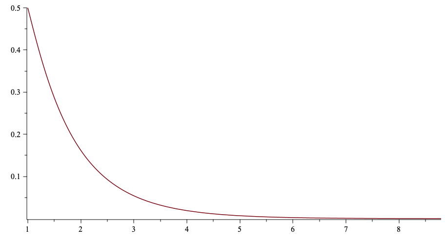
Figure 2 shows the parameter $\psi$ as a function of the average degree $\lambda$.

Figure 2. $\psi$, as function of $\lambda$.

Proof.

Let $J_{t}:=\boldsymbol{1}\{d(t)=0\}$, the indicator that vertex $t$ is a root and thus starts a new tree. Thus $N=\sum_{1}^{n}J_{t}$.

If $\theta_{1}>0$ (i.e., $\lambda>1$), then Theorem 2.4 shows that w.h.p. $d(t)>0$ in the interval $(1,n\theta_{1})$, except possibly close to the endpoints. Thus the DFS will find one giant tree of order $\approx\theta_{1}n$, possibly preceded by a few small trees, and, as we will see later in the proof, followed by many small trees. To obtain a precise estimate, we note that there exists a constant $c>0$ such that $\widetilde{\ell}(\theta)\geq\min\{c\theta,c(\theta_{1}-\theta)\}$ for $\theta\in[0,\theta_{1}]$. Hence, if $t\leq n\theta_{1}$ and $d(t)=0$, then $\widetilde{d}(t)\leq d(t)=0$ by (2.10) and, recalling (2.23),

$$M^{*}\geq n\widetilde{\ell}(t/n)\geq c\min\{t,n\theta_{1}-t\}.$$ (2.66)

Consequently, $d(t)=0$ with $t\leq n\theta_{1}$ implies $t\in[1,c^{-1}M^{*}]\cup[n\theta_{1}-c^{-1}M^{*},n\theta_{1}]$. The number of such $t$ is thus $O(M^{*}+1)=O_{L^{2}}(n^{1/2})$, using (2.23).

Let $T_{1}:=\lceil n\theta_{1}\rceil$. We have just shown that (the case $\theta_{1}=0$ is trivial)

$$\sum_{t=1}^{T_{1}-1}J_{t}=O_{L^{2}}(n^{1/2}).$$ (2.67)

It remains to consider $t\geq T_{1}$. For any integer $k\geq 0$, the conditional distribution of $\xi_{t}-k$ given $\xi_{t}\geq k$ equals the distribution of $\xi_{t}$. Hence, recalling (2.12),

$$\operatorname{\mathbb{E}{}}\bigl{[}(\xi_{t}-k)^{+}\bigr{]}=\operatorname{\mathbb{E}{}}\bigl{[}\xi_{t}-k\mid\xi_{t}\geq k\bigr{]}\operatorname{\mathbb{P}{}}(\xi_{t}\geq k)=\mu_{t}\operatorname{\mathbb{P}{}}(\xi_{t}-k\geq 0).$$ (2.68)

We use again the stochastic recursion (2.6). Let $\mathcal{F}_{t}$ be the $\sigma$-field generated by $\xi_{1},\dots,\xi_{t-1}$. Then $d(t)$ is $\mathcal{F}_{t}$-measurable, while $\xi_{t}$ is independent of $\mathcal{F}_{t}$. Hence, (2.6) and (2.68) yield

$$\operatorname{\mathbb{E}{}}\bigl{[}d(t+1)\mid\mathcal{F}_{t}\bigr{]} =\operatorname{\mathbb{E}{}}\bigl{[}d(t)+1-\xi_{t}\mid\mathcal{F}_{t}\bigr{]}+\operatorname{\mathbb{E}{}}\bigl{[}(\xi_{t}-1-d(t))^{+}\mid\mathcal{F}_{t}\bigr{]}$$

$$=d(t)+1-\mu_{t}+\mu_{t}\operatorname{\mathbb{P}{}}\bigl{[}\xi_{t}-1-d(t)\geq 0\mid\mathcal{F}_{t}\bigr{]}$$

$$=d(t)+1-\mu_{t}+\mu_{t}\operatorname{\mathbb{P}{}}\bigl{[}d(t+1)=0\mid\mathcal{F}_{t}\bigr{]}$$

$$=d(t)+1-\mu_{t}+\mu_{t}\operatorname{\mathbb{E}{}}\bigl{[}J_{t+1}\mid\mathcal{F}_{t}\bigr{]}.$$ (2.69)

We write $\Delta d(t):=d(t+1)-d(t)$ and $\overline{J}_{t}:=1-J_{t}$. Then (2.4) yields

$$\operatorname{\mathbb{E}{}}\bigl{[}\Delta d(t)-1+\mu_{t}\overline{J}_{t+1}\mid\mathcal{F}_{t}\bigr{]}=0.$$ (2.70)

Define

$$\mathcal{M}_{t}:=\sum_{i=1}^{t-1}\mu_{i}^{-1}\bigl{(}\Delta d(i)-1+\mu_{i}\overline{J}_{i+1}\bigr{)}=\sum_{i=1}^{t-1}\Bigl{(}\mu_{i}^{-1}\Delta d(i)-\mu_{i}^{-1}+\overline{J}_{i+1}\Bigr{)}.$$ (2.71)

Then $\mathcal{M}_{t}$ is $\mathcal{F}_{t}$-measurable, and (2.70) shows that $\mathcal{M}_{t}$ is a martingale. We have, with $\Delta\mathcal{M}_{t}:=\mathcal{M}_{t+1}-\mathcal{M}_{t}$, using (2.6),

$$|\Delta\mathcal{M}_{t}|\leq\mu_{t}^{-1}\bigl{\lvert}d(t+1)-d(t)-1\bigr{\rvert}+\overline{J}_{t+1}\leq\mu_{t}^{-1}\xi_{t}+1,$$ (2.72)

and thus, since $\pi_{t}\leq p<1$ for all $t$ by (2.8),

$$\operatorname{\mathbb{E}{}}\lvert\Delta\mathcal{M}_{t}\rvert^{2}\leq 2\mu_{t}^{-2}\operatorname{\mathbb{E}{}}\xi_{t}^{2}+2=2\Bigl{(}\frac{\pi_{t}}{1-\pi_{t}}\Bigr{)}^{2}\frac{1-\pi_{t}+(1-\pi_{t})^{2}}{\pi_{t}^{2}}+2=O(1).$$ (2.73)

Hence, uniformly for all $T\leq n$,

$$\operatorname{\mathbb{E}{}}\mathcal{M}_{T}^{2}=\sum_{t=1}^{T-1}\operatorname{\mathbb{E}{}}|\Delta\mathcal{M}_{t}|^{2}=O(T)=O(n).$$ (2.74)

The definition (2.71) yields

$$\mathcal{M}_{n}-\mathcal{M}_{T_{1}} =\sum_{t=T_{1}}^{n-1}\mu_{t}^{-1}\Delta d(t)-\sum_{t=T_{1}}^{n-1}\mu_{t}^{-1}+\sum_{t=T_{1}}^{n-1}\overline{J}_{t+1}.$$ (2.75)

By a summation by parts, and interpreting $\mu_{n}^{-1}:=0$,

$$\sum_{t=T_{1}}^{n-1}\mu_{t}^{-1}\Delta d(t)=\sum_{t=T_{1}+1}^{n}\bigl{(}\mu_{t-1}^{-1}-\mu_{t}^{-1}\bigr{)}d(t)-\mu_{T_{1}}^{-1}d(T_{1}).$$ (2.76)

As $t$ increases, $\mu_{t}$ increases by (2.12), and thus $\mu_{t-1}^{-1}-\mu_{t}^{-1}>0$. Hence, (2.76) implies

$$\Bigl{\lvert}\sum_{t=T_{1}}^{n-1}\mu_{t}^{-1}\Delta d(t)\Bigr{\rvert} \leq\sum_{t=T_{1}+1}^{n}\bigl{(}\mu_{t-1}^{-1}-\mu_{t}^{-1}\bigr{)}\sup_{i>T_{1}}|d(t)|+\mu_{T_{1}}^{-1}|d(T_{1})|\leq 2\mu_{T_{1}}^{-1}\sup_{i\geq T_{1}}|d(t)|$$

$$=O_{L^{2}}(n^{1/2})$$ (2.77)

by (2.20), since $\widetilde{\ell}^{+}(t/n)=0$ for $t\geq T_{1}\geq n\theta_{1}$. Furthermore, (2.74) shows that $\mathcal{M}_{n},\mathcal{M}_{T_{1}}=O_{L^{2}}(n^{1/2})$. Hence, (2.75) yields, using (2.12),

$$\sum_{t=T_{1}+1}^{n}J_{t} =n-T_{1}-\sum_{t=T_{1}+1}^{n}\overline{J}_{t}=n-T_{1}-\sum_{t=T_{1}}^{n-1}\mu_{t}^{-1}+O_{L^{2}}(n^{1/2})$$

$$=n-T_{1}-\sum_{t=T_{1}}^{n-1}\lambda(1-t/n)+O_{L^{2}}(n^{1/2})=n\psi+O_{L^{2}}(n^{1/2}),$$ (2.78)

where

$$\psi:=1-\theta_{1}-\int_{\theta_{1}}^{1}\lambda{(1-x)}\,\mathrm{d}x=1-\theta_{1}-\frac{\lambda}{2}(1-\theta_{1})^{2}.$$ (2.79)

The result follows by (2.4) and (2.67). ∎

The arguments in the proof of Theorem 2.12 show that in the supercritical case $\lambda>1$, the DFS w.h.p. find first possibly a few small trees, then a giant tree containing all $v_{t}$ with $O_{L^{2}}(n^{1/2})\leq t\leq\theta_{1}n+O_{L^{2}}(n^{1/2})$, and then a large number of small trees. We give some details in the following lemma and theorem.

Lemma 2.13.

Let $(a,b)$ be a fixed interval with $0\leq a<b\leq 1$ and $b>\theta_{1}$. Then w.h.p. there exists a root $v_{t}$ in the depth-first forest with $t/n\in(a,b)$.

Proof.

By increasing $a$, we may assume that $\theta_{1}<a<b\leq 1$. Then, cf. (2.15), $\widetilde{\ell}^{\prime}(a)<\widetilde{\ell}^{\prime}(\theta_{1})\leq 0$ and thus $\lambda(1-a)<1$. Hence, the argument yielding (2.4) in the proof of Theorem 2.12 yields also

$$\sum_{t=\lceil an\rceil}^{\lfloor bn\rfloor}J_{t} =bn-an-\sum_{t=\lceil an\rceil}^{\lfloor bn\rfloor}\lambda(1-t/n)+O_{L^{2}}(n^{1/2})=cn+O_{L^{2}}(n^{1/2}),$$ (2.80)

with $c>(b-a)(1-\lambda(1-a))>0$. Hence, w.h.p. there are many roots $v_{t}$ with $t\in(an,bn)$. ∎

Theorem 2.14.

Let $\mathbf{T}_{1}$ be the largest tree in the depth-first forest.

1. If $\lambda\leq 1$, then $|\mathbf{T}_{1}|=o_{\mathrm{p}}(n)$.

2. If $\lambda>1$, then $|\mathbf{T}_{1}|=\theta_{1}n+O_{L^{2}}(n^{1/2})$. Furthermore, the second largest tree has order $|\mathbf{T}_{2}|=o_{\mathrm{p}}(n)$.

Proof.

Let $\varepsilon>0$. By covering $[\theta_{1},1]$ with a finite number of intervals of length $<\varepsilon/2$, it follows from Lemma 2.13 that w.h.p. every tree $\mathbf{T}$ having a root $v_{t}$ with $t>(\theta_{1}-\varepsilon/2)n$ has $|\mathbf{T}|\leq\varepsilon n$.

In particular, if $\lambda\leq 1$, so $\theta_{1}=0$, this applies to all trees, and thus w.h.p. $|\mathbf{T}_{1}|\leq\varepsilon n$, which proves (i).

Suppose now $\lambda>1$. Consider the tree $\mathbf{T}$ in the depth-first forest that contains $v_{\lfloor n\theta_{0}\rfloor}$, denote its root by $v_{r}$ and let $v_{s}$ be its last vertex. By the proof of Theorem 2.12, $d(t)>0$ for $O_{L^{2}}(n^{1/2})\leq t\leq\theta_{1}n-O_{L^{2}}(n^{1/2})$, and thus $r=O_{L^{2}}(n^{1/2})$ and $s\geq\theta_{1}n-O_{L^{2}}(n^{1/2})$.

On the other hand, let $\theta^{*}\in(\theta_{1},1)$. If $s\geq\theta_{1}n$, let $u:=\min\{s,\lfloor\theta^{*}n\rfloor\}$. Since $r/n\leq\theta_{0}$, we have $\widetilde{\ell}(r/n)\geq 0$. Furthermore, (2.10) implies that $\widetilde{d}(t)>\min_{j\leq t}\widetilde{d}(j)=\widetilde{d}(r)$ for $t\in(r,s]$, and thus $\widetilde{d}(u)>\widetilde{d}(r)$. Hence, by (2.23),

$$-n\widetilde{\ell}(u/n)\leq n\widetilde{\ell}(r/n)-n\widetilde{\ell}(u/n)\leq 2M^{*}+\widetilde{d}(r)-\widetilde{d}(u)\leq 2M^{*}=O_{L^{2}}(n^{1/2}).$$ (2.81)

Since $\widetilde{\ell}(\theta_{1})=0$ and $\widetilde{\ell}^{\prime}(\theta)\leq-c<0$ for $\theta\geq\theta_{1}$, it follows that $u\leq\theta_{1}n+O_{L^{2}}(n^{1/2})$, and thus $s\leq\theta_{1}n+O_{L^{2}}(n^{1/2})$.

Consequently, $s=\theta_{1}n+O_{L^{2}}(n^{1/2})$, and thus $|\mathbf{T}|=s-r+1=\theta_{1}n+O_{L^{2}}(n^{1/2})$. Furthermore, any tree found before $\mathbf{T}$ has order $\leq r=o_{\mathrm{p}}(n)$. The first part of the proof now shows that for every $\varepsilon>0$, there is w.h.p. no tree other than $|\mathbf{T}|$ of order $>\varepsilon n$. Hence, w.h.p. $\mathbf{T}$ is the largest tree, and (ii) follows. ∎

Remark 2.15.

As said in Remark 2.3, $\theta_{1}$, the asymptotic fraction of vertices in the giant tree, equals the survival probability of a Galton–Watson process with $\operatorname{Po}(\lambda)$ offspring distribution. Heuristically, this may be explained by the following argument, well known from similar situations. Start at a random vertex and follow the arcs backwards. The indegree of a given vertex is asymptotically $\operatorname{Po}(\lambda)$, and the process of exploring backwards from a vertex may be approximated by a Galton–Watson process with this offspring distribution. Hence, the probability of a “large” backwards process converges to the survival probability $\theta_{1}$. It seems reasonable that most vertices in the giant tree have a large backwards process, while most vertices outside the giant have a small backwards process.

Note also that the asymptotic size of the giant tree thus equals the asymptotic size of the giant component in an undirected Erdős–Rényi random graph $G(n,\lambda/n)$, which heuristically is given by the same argument. (See also Remark 1.1 and [11].)

2.5. Types of arcs

Recall from the introduction the classification of the arcs in the digraph $G$. Since we assume that the outdegrees are $\operatorname{Ge}(1-p)$ and independent, the total number of arcs, $M$ say, has a negative binomial distribution with mean $\lambda n$, and, by a weak version of the law of large numbers,

$$M=\lambda n+O_{L^{2}}(n^{1/2}).$$ (2.82)

In the following theorem, we give the asymptotics of the number of arcs of each type.

Theorem 2.16.

Let $L$, $T$, $B$, $F$ and $C$ be the numbers of loops, tree arcs, back arcs, forward arcs, and cross arcs in the random digraph. Then

$$L =O_{L^{2}}(1),$$ (2.83)

$$T =\tau n+O_{L^{2}}(n^{1/2}),$$ (2.84)

$$B =\beta n+O_{L^{2}}(n^{1/2}),$$ (2.85)

$$F =\varphi n+O_{L^{2}}(n^{1/2}),$$ (2.86)

$$C =\chi n+O_{L^{2}}(n^{1/2}),$$ (2.87)

where

$$\tau :=\chi:=1-\psi=\theta_{1}+\frac{\lambda}{2}(1-\theta_{1})^{2},$$ (2.88)

$$\beta :=\varphi:=\lambda\alpha=(\lambda-1)\theta_{1}-\frac{\lambda}{2}\theta_{1}^{2}.$$ (2.89)

Proof.

Let $\eta_{t}$ be the number of arcs from $v_{t}$, and let $\eta^{<}_{t},\eta^{=}_{t},\eta^{>}_{t}$ be the numbers of these arcs that lead to some $v_{u}$ with $u<t$, $u=t$ and $u>t$, respectively. Then

$$L=\sum_{t=1}^{n}\eta^{=}_{t}.$$ (2.90)

Furthermore, an arc $v_{t}v_{u}$ with $u>t$ is either a tree arc or a forward arc; conversely, every tree arc or forward arc is of this type. Consequently,

$$T+F =\sum_{t=1}^{n}\eta^{>}_{t}.$$ (2.91)

Similarly, or by (2.90) and (2.91),

$$B+C =\sum_{t=1}^{n}\eta^{<}_{t}.$$ (2.92)

Conditioned on $\eta_{t}$, $\eta^{<}_{t}$ has a binomial distribution $\operatorname{Bin}(\eta_{t},(t-1)/n)$, since each arc has probability $(t-1)/n$ to go to a vertex $v_{u}$ with $u<t$. In general, if $X\sim\operatorname{Bin}(m,p)$, then $\operatorname{\mathbb{E}{}}X=mp$ and $\operatorname{\mathbb{E}{}}X^{2}=\operatorname{Var}X+(\operatorname{\mathbb{E}{}}X)^{2}=mp(1-p)+(mp)^{2}$. Hence, by first conditioning on $\eta_{t}$,

$$\operatorname{\mathbb{E}{}}\eta^{<}_{t} =\operatorname{\mathbb{E}{}}\Bigl{[}\eta_{t}\frac{t-1}{n}\Bigr{]}=\lambda\frac{t-1}{n},$$ (2.93)

$$\operatorname{Var}\eta^{<}_{t} \leq\operatorname{\mathbb{E}{}}\bigl{[}(\eta^{<}_{t})^{2}\bigr{]}=\operatorname{\mathbb{E}{}}\Bigl{[}\eta_{t}\frac{t-1}{n}\Bigl{(}1-\frac{t-1}{n}\Bigr{)}+\eta_{t}^{2}\Bigl{(}\frac{t-1}{n}\Bigr{)}^{2}\Bigr{]}=O(1).$$ (2.94)

Furthermore, the random variables $\eta^{<}_{t}$, $t=1,\dots,n$, are independent. Hence, (2.92) yields

$$\operatorname{\mathbb{E}{}}B+\operatorname{\mathbb{E}{}}C =\sum_{t=1}^{n}\operatorname{\mathbb{E}{}}\eta^{<}_{t}=\lambda\sum_{t=1}^{n}\frac{t-1}{n}=\frac{\lambda}{2}(n-1),$$ (2.95)

$$\operatorname{Var}[B+C] =\sum_{t=1}^{n}\operatorname{Var}\eta^{<}_{t}=O(n),$$ (2.96)

and thus

$$B+C=\operatorname{\mathbb{E}{}}[B+C]+O_{L^{2}}(n^{1/2})=\frac{\lambda}{2}n+O_{L^{2}}(n^{1/2}).$$ (2.97)

The same argument with (2.91) yields

$$\operatorname{\mathbb{E}{}}T+\operatorname{\mathbb{E}{}}F =\frac{\lambda}{2}(n-1),$$ (2.98)

$$\operatorname{Var}[F+T] =O(n),$$ (2.99)

$$F+T =\frac{\lambda}{2}n+O_{L^{2}}(n^{1/2}).$$ (2.100)

Similarly, conditioned on $\eta_{t}$, we have $\eta^{=}\sim\operatorname{Bin}(\eta_{t},1/n)$, and we find

$$\operatorname{\mathbb{E}{}}L =\sum_{t=1}^{n}\operatorname{\mathbb{E}{}}\eta^{=}_{t}=n\lambda\frac{1}{n}=\lambda,$$ (2.101)

$$\operatorname{Var}{L} =\sum_{t=1}^{n}\operatorname{Var}\eta^{=}_{t}=O(1),$$ (2.102)

$$L =\lambda+O_{L^{2}}(1)=O_{L^{2}}(1).$$ (2.103)

This proves (2.83). We prove (2.84)–(2.87) one by one.

$T$: In any forest, the number of vertices equals the number of edges + the number of trees. Hence, $T=n-N$, where $n$ is the number of trees in the depth-first forest, and thus Theorem 2.12 implies (2.84) with $\tau=1-\psi$ given by (2.88).

$B$: Let $B_{t}$ be the number of back arcs from $v_{t}$; thus $B=\sum_{1}^{n}B_{t}$. Let $\mathcal{F}_{t}$ be the $\sigma$-field generated by all arcs from $v_{i}$, $i\leq t$ (i.e., by the outdegrees $\eta_{i}$ and the endpoints of all these arcs); note that this includes complete information on the DFS until $v_{t+1}$ is found, but also on some further arcs (the future arcs from the ancestors of $v_{t+1}$). Then $d(t)$ is $\mathcal{F}_{t-1}$-measurable and $B_{t}$ is $\mathcal{F}_{t}$-measurable. Moreover, $\eta_{t}$ is independent of $\mathcal{F}_{t-1}$. Thus, conditioned on $\mathcal{F}_{t-1}$, we still have $\eta_{t}\sim\mathbf{P}$; we also know $d(t)$, and each arc from $v_{t}$ is a back arc with probability $d(t)/n$. Hence, $\operatorname{\mathbb{E}{}}\bigl{[}B_{t}\mid\mathcal{F}_{t-1},\eta_{t}\bigr{]}=\eta_{t}d(t)/n$, and consequently

$$\operatorname{\mathbb{E}{}}\bigl{[}B_{t}\mid\mathcal{F}_{t-1}\bigr{]}=\operatorname{\mathbb{E}{}}\Bigl{[}\eta_{t}\frac{d(t)}{n}\mid\mathcal{F}_{t-1}\Bigr{]}=\lambda\frac{d(t)}{n}.$$ (2.104)

Similarly, since, as above, $X\sim\operatorname{Bin}(m,p)$ implies $\operatorname{\mathbb{E}{}}X^{2}=mp(1-p)+(mp)^{2}$,

$$\operatorname{\mathbb{E}{}}\bigl{[}B_{t}^{2}\mid\mathcal{F}_{t-1}\bigr{]}=\operatorname{\mathbb{E}{}}\Bigl{[}\eta_{t}\frac{d(t)}{n}\Bigl{(}1-\frac{d(t)}{n}\Bigr{)}+\Bigl{(}\eta_{t}\frac{d(t)}{n}\Bigr{)}^{2}\mid\mathcal{F}_{t-1}\Bigr{]}=O(1).$$ (2.105)

Define $\Delta Z_{t}:=B_{t}-\lambda d(t)/n$ and $Z_{t}:=\sum_{1}^{t}\Delta Z_{i}$. Then (2.104) shows that $\operatorname{\mathbb{E}{}}\bigl{[}\Delta Z_{t}\mid\mathcal{F}_{t}\bigr{]}=0$, and thus $(Z_{i})_{0}^{n}$ is a martingale, with $Z_{0}=0$. Hence, $\operatorname{\mathbb{E}{}}Z_{n}=0$. Furthermore, (2.104) implies $\operatorname{\mathbb{E}{}}\bigl{[}(\Delta Z_{t})^{2}\bigr{]}=\operatorname{\mathbb{E}{}}\bigl{[}(B_{t}-\operatorname{\mathbb{E}{}}[B_{t}\mid\mathcal{F}_{t-1}])^{2}\bigr{]}\leq\operatorname{\mathbb{E}{}}\bigl{[}B_{t}^{2}\bigr{]}$, and thus by (2.105),

$$\operatorname{\mathbb{E}{}}\bigl{[}Z_{n}^{2}\bigr{]}=\operatorname{Var}\bigl{[}Z_{n}\bigr{]}=\sum_{t=1}^{n}\operatorname{\mathbb{E}{}}\bigl{[}(\Delta Z_{t})^{2}\bigr{]}\leq\sum_{t=1}^{n}\operatorname{\mathbb{E}{}}\bigl{[}B_{t}^{2}\bigr{]}=O(n).$$ (2.106)

Consequently, $Z_{n}=O_{L^{2}}(n^{1/2})$, and thus

$$B=\sum_{t=1}^{n}B_{t}=Z_{n}+\sum_{t=1}^{n}\lambda\frac{d(t)}{n}=\lambda\overline{d}+Z_{n}=\lambda\overline{d}+O_{L^{2}}(n^{1/2}).$$ (2.107)

Finally, (2.107) and Corollary 2.6 yield

$$B=\lambda\overline{d}+O_{L^{2}}(n^{1/2})=\lambda\alpha n+O_{L^{2}}(n^{1/2}),$$ (2.108)

which shows (2.85) with $\beta=\lambda\alpha$ as in (2.89), recalling (2.38).

$F$: By (2.100) and (2.84), we have (2.86) with $\varphi=\frac{\lambda}{2}-\tau$, which agrees with (2.89) by (2.88) and a simple calculation. In particular, $\varphi=\beta$.

$C$: Similarly, it follows from (2.97) and (2.85) that we have (2.87) with $\chi:=\lambda/2-\beta$. Since we have found $\beta=\varphi$, and we always have $\tau+\varphi=\lambda/2=\beta+\chi$, see (2.97) and (2.100), we thus have $\chi=\tau$, and thus (2.88) holds. ∎

Note that $T+F$ and $B+C$ are asymptotically normal; this follows immediately from (2.91) and (2.92) by the central limit theorem.

Conjecture 2.17.

All four variables $T,B,F,C$ are (jointly) asymptotically normal.

The equalitites $\tau=\chi$ and $\beta=\varphi$ mean asymptotic equality of the corresponding expectations of numbers of arcs. In fact, there are exact equalities.

Theorem 2.18.

For any $n$, $\operatorname{\mathbb{E}{}}T=\operatorname{\mathbb{E}{}}C$ and $\operatorname{\mathbb{E}{}}B=\operatorname{\mathbb{E}{}}F=\lambda\operatorname{\mathbb{E}{}}\overline{d}$.

Proof.

Let $v,w$ be two distinct vertices. If the DFS finds $w$ as a descendant of $v$, then there will later be $\operatorname{Ge}(1-p)$ arcs from $w$, and each has probability $1/n$ of being a back arc to $v$. Similarly, there will be $\operatorname{Ge}(1-p)$ future arcs from $v$, and each has probability $1/n$ of being a forward arc to $w$. Hence, if $I_{vw}$ is the indicator that $w$ is a descendant of $v$, and $B_{vw}$ [$F_{vw}$] is the number of back [forward] arcs $vw$, then

$$\operatorname{\mathbb{E}{}}B_{wv}=\operatorname{\mathbb{E}{}}F_{vw}=\frac{\lambda}{n}\operatorname{\mathbb{E}{}}I_{vw}.$$ (2.109)

Summing over all pairs of distinct $v$ and $w$, we obtain

$$\operatorname{\mathbb{E}{}}B=\operatorname{\mathbb{E}{}}F=\frac{\lambda}{n}\operatorname{\mathbb{E}{}}\sum_{w}\sum_{v\neq w}I_{vw}=\frac{\lambda}{n}\operatorname{\mathbb{E}{}}\sum_{w}d(w)=\lambda\operatorname{\mathbb{E}{}}\overline{d}.$$ (2.110)

Finally, $\operatorname{\mathbb{E}{}}T+\operatorname{\mathbb{E}{}}F=\operatorname{\mathbb{E}{}}C+\operatorname{\mathbb{E}{}}B$ by (2.98) and (2.95), and thus (2.110) implies $\operatorname{\mathbb{E}{}}T=\operatorname{\mathbb{E}{}}C$. ∎

Remark 2.19.

Knuth [13] conjectures, based on exact calculation of generating functions for small $n$, that, much more strongly, $B$ and $F$ have the same distribution for every $n$. (Note that $T$ and $C$ do not have the same distribution; we have $T\leq n-1$, while $C$ may take arbitrarily large values.)

Remark 2.20.

A simple argument with generating functions shows that the number of loops at a given vertex $v$ is $\operatorname{Ge}(1-p/(n-np+p))$; these numbers are independent, and thus $L\sim\operatorname{NegBin}\bigl{(}n,1-p/(n-np+p)\bigr{)}$ with $\operatorname{\mathbb{E}{}}L=p/(1-p)=\lambda=O(1)$ and $\operatorname{Var}(L)=p(1-p+p/n)/(1-p)^{2}=\lambda(1+\lambda/n)=O(1)$ [13]. Moreover, it is easily seen that asymptotically, $L$ has a Poisson distribution, $L\overset{\mathrm{d}}{\longrightarrow}\operatorname{Po}(\lambda)$ as ${n\to\infty}$.

3. Depth, trees and arc analysis in the shifted geometric outdegree distribution

In this section, the outdegree distribution is $\operatorname{Ge}_{1}(1-p)=1+\operatorname{Ge}(1-p)$. Thus we now have the mean

$$\lambda=\frac{1}{1-p}.$$ (3.1)

Thus $\lambda>1$, and only the supercritical case occurs. As in Section 2, the depth $d(t)$ is a Markov chain given by (2.6), but the distribution of $\xi_{t}$ is now different. The probability (2.2) is replaced by $(1-t/n)/(1-pt/n)$, but the number of future arcs from an ancestor is still $\operatorname{Ge}(1-p)$, and, with $\theta:=t/n$,

$$\operatorname{\mathbb{P}{}}\bigl{(}\xi_{t}=k\bigr{)}=\begin{cases}\overline{\pi}_{t}:=\frac{1-\theta}{1-p\theta},&k=0,\\ (1-\overline{\pi}_{t})(1-\pi_{t})^{k-1}\pi_{t},&k\geq 1,\end{cases}$$ (3.2)

where $\pi_{t}=p\overline{\pi}_{t}$ is as in (2.8). The rest of the analysis does not change, and the results in Theorems 2.4–2.16 still hold, but we get different values for many of the constants.

We now have

$$\operatorname{\mathbb{E}{}}\xi_{t}=\overline{\mu}_{t}:=\frac{(1-p)\theta}{p(1-\theta)}$$ (3.3)

and instead of (2.14) we have $\operatorname{\mathbb{E}{}}\widetilde{d}(t)=n\widetilde{\ell}(\theta)+O(1)$ where now $\widetilde{\ell}(\theta)$ takes the new value

$$\widetilde{\ell}(\theta) :=\int_{0}^{\theta}\left(1-\frac{(1-p)x}{p(1-x)}\right)\,\mathrm{d}x=\frac{1}{p}\theta+\frac{1-p}{p}\log(1-\theta)$$

$$\phantom{:}=\frac{1}{p}\bigl{(}\theta+\lambda^{-1}\log(1-\theta)\bigr{)}.$$ (3.4)

Note that $\widetilde{\ell}(\theta)$ in (3) is proportional to (2.15) for the (unshifted) geometric distribution with the same $\lambda$, but larger by a factor $1/p$. Figures 3 and 4 show $\widetilde{\ell}(\theta)$ for both geometric distributions with the same $p$ ($0.6$) and the same $\lambda$ (2.0), respectively.

Figure 3. $\widetilde{\ell}(\theta)$, the asymptotic search depth, for geometric distribution $\operatorname{Ge}(1-p)$ (solid) and shifted geometric distribution $\operatorname{Ge}_{1}(1-p)$ (dashed) with $p=0.6$ and thus $\lambda=1.5$ and $\lambda=2.5$, respectively.

Figure 4. $\widetilde{\ell}(\theta)$, the asymptotic search depth, for geometric distribution $\operatorname{Ge}(1-p)$ (solid) and shifted geometric distribution $\operatorname{Ge}_{1}(1-p)$ (dashed) with $p=2/3$ and $1/2$, respectively, and thus $\lambda=2$.

Note that $\widetilde{\ell}(\theta_{1})=0$ still gives (2.17) and (2.18), now with $\lambda=1/(1-p)$ as in (3.1), and that $\lambda>1$ so $\theta_{1}>0$ for every $p$. Differentiating (3) shows that the maximum point $\theta_{0}=p>0$, which again is given by (2.16). Straightforward calculations yield

$$\upsilon :=\widetilde{\ell}(p)=1+\frac{1-p}{p}\log(1-p)=1-\frac{1}{\lambda-1}\log\lambda,$$ (3.5)

$$\alpha :=\frac{1}{p}\left(\frac{\theta_{1}^{2}}{2}-\frac{1}{\lambda}\bigl{(}(1-\theta_{1})\log(1-\theta_{1})+\theta_{1}\bigr{)}\right)=\theta_{1}-\frac{\theta_{1}^{2}}{2p}.$$ (3.6)

Furthermore, (3.2) yields by a simple calculation, with $\theta:=t/n$,

$$\operatorname{Var}\xi_{t}=\frac{(1-p)^{2}}{p^{2}(1-\theta)^{2}}+\frac{1-p}{p(1-\theta)}-\frac{1-p}{p^{2}}.$$ (3.7)

Hence, (2.44) holds with (2.45) replaced by

$$v(\theta) :=\int_{0}^{\theta}\Bigl{(}\frac{(1-p)^{2}}{p^{2}(1-x)^{2}}+\frac{1-p}{p(1-x)}-\frac{1-p}{p^{2}}\Bigr{)}\,\mathrm{d}x$$

$$\phantom{:}=\frac{(1-p)^{2}\theta}{p^{2}(1-\theta)}-\frac{1-p}{p}\log(1-\theta)-\frac{1-p}{p^{2}}\theta,$$ (3.8)

and then Lemma 2.8 and Theorem 2.10 hold with this $v(\theta)$.

Consequently, Theorem 2.11 holds with

$$\sigma^{2}:=v(p)=-\frac{1-p}{p}\log(1-p).$$ (3.9)

In the proof of Theorem 2.12, (2.68) for $k\geq 1$ still holds with $\mu_{t}$ given by (2.12) (except for the formula with $\lambda$), and thus (2.4) is replaced by, using (3.3),

$$\operatorname{\mathbb{E}{}}\bigl{[}d(t+1)\mid\mathcal{F}_{t}\bigr{]} =d(t)+1-\overline{\mu}_{t}+\mu_{t}\operatorname{\mathbb{E}{}}\bigl{[}J_{t+1}\mid\mathcal{F}_{t}\bigr{]}.$$ (3.10)

The rest of the proof remains the same with minor modifications, and leads to, instead of (2.4), with $\theta:=t/n$,

$$\sum_{t=T_{1}+1}^{n}J_{t} =\sum_{t=T_{1}}^{n-1}\frac{\overline{\mu}_{t}-1}{\mu_{t}}+O_{L^{2}}(n^{1/2})=\sum_{t=T_{1}}^{n-1}\frac{\frac{(1-p)\theta}{p(1-\theta)}-1}{\frac{1-p}{p(1-\theta)}}+O_{L^{2}}(n^{1/2})$$

$$=\sum_{t=T_{1}}^{n-1}\bigl{(}1-\lambda(1-\theta)\bigr{)}+O_{L^{2}}(n^{1/2}),$$ (3.11)

and thus Theorem 2.12 holds with

$$\psi:=\int_{\theta_{1}}^{1}\bigl{(}1-\lambda(1-x)\bigr{)}\,\mathrm{d}x=1-\theta_{1}-\frac{\lambda}{2}(1-\theta_{1})^{2},$$ (3.12)

just as in (2.65).

In the proof of Theorem 2.16, (2.108) still holds, and we obtain (2.85) with $\beta=\lambda\alpha$, and then (2.87) with $\chi=\lambda/2-\beta$ just as before (but recall that $\alpha$ now is different). On the other hand, now the expected numbers of back and forward arcs differ since $\operatorname{\mathbb{E}{}}B=\lambda\operatorname{\mathbb{E}{}}\overline{d}\sim\lambda\alpha n$ and $\operatorname{\mathbb{E}{}}F=(\lambda-1)\operatorname{\mathbb{E}{}}\overline{d}\sim(\lambda-1)\alpha n$ because the average number of future arcs at a vertex after a descendant has been created is $\lambda-1$. The asymptotic formula (2.84) holds as above with $\tau:=1-\psi$; hence (2.98) implies that (2.86) holds too, with $\varphi=\lambda/2-\tau$; as just noted, we now have $\varphi=(\lambda-1)\alpha\neq\beta$. Collecting these constants, we see that Theorem 2.16 holds with

$$\tau :=1-\psi=\theta_{1}+\frac{\lambda}{2}(1-\theta_{1})^{2},$$ (3.13)

$$\beta :=\lambda\alpha=\lambda\theta_{1}-\frac{\lambda}{2p}\theta_{1}^{2}=\lambda\theta_{1}-\frac{\lambda^{2}}{2(\lambda-1)}\theta_{1}^{2},$$ (3.14)

$$\varphi :=(\lambda-1)\alpha=(\lambda-1)\theta_{1}-\frac{\lambda}{2}\theta_{1}^{2}=\frac{\lambda}{2}-\tau,$$ (3.15)

$$\chi :=\frac{\lambda}{2}-\beta=\frac{\lambda}{2}(1-\theta_{1})^{2}+\frac{\lambda}{2(\lambda-1)}\theta_{1}^{2}.$$ (3.16)

Thus the equality $\beta=\varphi$ and the equality of the expected number of back and forward arcs in Theorems 2.16 and Theorem 2.18 was an artefact of the geometric degree distribution. Similarly, $\chi=\lambda/2-\beta<\lambda/2-\varphi=\tau$, and the equality of the expected numbers of tree arcs and cross arcs in Theorem 2.18 also does not hold.

We summarize the results above.

Theorem 3.1.

Let the outdegree distribution $\mathbf{P}$ be the shifted geometric distribution $\operatorname{Ge}_{1}(p)$ with $p\in(0,1)$. Then Theorems 2.4–2.16 hold, with the constants now having the values described above (and always $\lambda>1$), while Theorem 2.18 does not hold.

4. A general outdegree distribution: stack size

In this section, we consider a general outdegree distribution $\mathbf{P}$, with mean $\lambda$ and finite variance.

When the outdegree distribution is general, the depth does not longer follow a simple Markov chain, since we would have to keep track of the number of children seen so far at each level of the branch of the tree toward the current vertex. Instead we get back a Markov chain if we instead of the depth consider the stack size $I(t)$, defined as follows.

The DFS can be regarded as keeping a stack of unexplored arcs, for which we have seen the start vertex but not the endpoint. The stack evolves as follows:

1. If the stack is empty, pick a new vertex $v$ that has not been seen before (if there is no such vertex, we have finished). Otherwise, pop the last arc from the stack, and reveal its endpoint $v$ (which is uniformly random over all vertices). If $v$ already is seen, repeat.

2. ($v$ is now a new vertex) Reveal the outdegree $\eta$ of $v$ and add to the stack $\eta$ new arcs from $v$, with unspecified endpoints. GOTO S1.

Let again $v_{t}$ be the $t$-th vertex seen by the DFS, and let $I(t)$ be the size of the stack when $v_{t}$ is found (but before we add the arcs from $v_{t}$). It can easily be seen that $I(t)$ will be a Markov chain, similar (but not identical) to the depth process $d(t)$ in the geometric case studied above. Moreover, it is possible to recover the depth of the vertices from the stack size process, which makes it possible to extend many of the results above, although sometimes with less precision. For details, see [11].

References

- [1]
- Aldous [1997] David Aldous. Brownian excursions, critical random graphs and the multiplicative coalescent. Ann. Probab. 25 (1997), no. 2, 812–854.
- [3] Krishna B. Athreya & Peter E. Ney. Branching Processes. Springer-Verlag, Berlin, 1972.
- Billingsley [1968] Patrick Billingsley. Convergence of Probability Measures. Wiley, New York, 1968.
- Diskin and Krivelevich [2021+] Sahar Diskin & Michael Krivelevich. On the performance of the Depth First Search algorithm in supercritical random graphs. Preprint, 2021. arXiv:2111.07345
- Enriquez, Faraud and Ménard [2020] Nathanaël Enriquez, Gabriel Faraud & Laurent Ménard. Limiting shape of the depth first search tree in an Erdős-Rényi graph. Random Structures Algorithms 56 (2020), no. 2, 501–516.
- [7] Allan Gut. Probability: A Graduate Course, 2nd ed., Springer, New York, 2013.
- [8] Jean Jacod & Albert N. Shiryaev. Limit Theorems for Stochastic Processes. Springer-Verlag, Berlin, 1987.
- [9] Svante Janson. Orthogonal decompositions and functional limit theorems for random graph statistics. Mem. Amer. Math. Soc., 111, no. 534, Amer. Math. Soc., Providence, R.I., 1994.
- Janson [2004] Svante Janson. Functional limit theorems for multitype branching processes and generalized Polya urns. Stoch. Process. Appl. 110 (2004), 177–245.
- [11] Svante Janson & Philippe Jacquet. Depth-First Search performance in random digraphs with general outdegree distributions. In preparation.
- Kallenberg [2002] Olav Kallenberg. Foundations of Modern Probability. 2nd ed., Springer-Verlag, New York, 2002.
-
Knuth [2022+]
Donald E. Knuth.
The Art of Computer Programming, Section 7.4.1.2
(Preliminary draft, 13 February 2022).
http://cs.stanford.edu/~knuth/fasc12a.ps.gz - [14] Michael Krivelevich & Benny Sudakov. The phase transition in random graphs: a simple proof. Random Structures Algorithms 43 (2013), no. 2, 131–138.