Mixture of von Mises-Fisher distribution with sparse prototypes

Abstract

Mixtures of von Mises-Fisher distributions can be used to cluster data on the unit hypersphere. This is particularly adapted for high-dimensional directional data such as texts. We propose in this article to estimate a von Mises mixture using a $l_{1}$ penalized likelihood. This leads to sparse prototypes that improve clustering interpretability. We introduce an expectation-maximisation (EM) algorithm for this estimation and explore the trade-off between the sparsity term and the likelihood one with a path following algorithm. The model’s behaviour is studied on simulated data and, we show the advantages of the approach on real data benchmark. We also introduce a new data set on financial reports and exhibit the benefits of our method for exploratory analysis.

[inst2]organization=Universite Paris Dauphine-PSL - CEREMADE UMR 7534,city=Paris, country=France

[inst1]organization=Universite Paris 1 Pantheon-Sorbonne - Laboratoire SAMM EA 4543,city=Paris, country=France

1 Introduction

High dimensional data are difficult to study as many classical machine learning techniques are impaired by the so called curse of dimensionality [4, 12]. One of the manifestation of this curse is the tendency of distances to concentrate: pairwise distances between observations have both a large mean and a small variance (see [5, 17]). This shows also that a multivariate Gaussian distribution is mostly concentrated on a central sphere.

As a consequence, the classical Gaussian mixture model is generally not adapted to high-dimensional data and numerous variants have been proposed to cluster such data, see e.g. [8, 26, 34] and in particular the survey [7]. One of the main strategy to adapt Gaussian mixtures to high dimensional settings is to reduce in some way the relevant dimensions of the components of the mixture. For instance in [8], the authors propose a method in which each component of the Gaussian mixture is associated to a specific low-dimensional projection. In this sense, it can be seen as a generalization of the principle of principal component analysis mixture [32].

This strategy can be applied in a more direct way for a particular case of high-dimensional data, the so-called directional data [24] for which the correlation between two vectors is more informative than the norm of their difference (i.e. the Euclidean distance). This type of data appears naturally in the classical vector representation of texts, as well as microarray analysis and recommender systems. In addition of the need for a specific similarity measure, those data have frequently more variables than the number of observations. This constrains strongly the type of Gaussian mixture than can be considered as e.g. the covariance matrix of the data is degenerate. For those data Gaussian-type models are doubly non adapted: they suffer from the adverse effects of high dimensionality and are based on a non adapted underlying metric.

A natural way to handle directional data is to carry out a normalisation that places them on the unit hyper-sphere. Notice that the concentration phenomenon recalled above has already a tendency to push all observations on such a hyper-sphere. This gives to the directional model a broader application domain in high dimensional spaces. Then one can use clustering techniques that address specifically the fact the data are spherical, such as spherical k-means [15]. In particular, the von Mises-Fisher distribution can be used as the building block for mixture models for directional data.

The von Mises-Fisher (vMF) distribution is a probability distribution on the unit hypersphere which is close to the wrapped version of the normal distribution but is also simpler and more tractable. It uses two parameters: a directional mean and a concentration parameter $\kappa$ which play similar roles as the mean and the precision (inverse of the variance) in the Gaussian distribution. Its density is given by

$$f(\boldsymbol{x}|\boldsymbol{\mu},\kappa)=c_{d}(\kappa)\exp^{\kappa\boldsymbol{\mu}^{T}\boldsymbol{x}},$$

where $c_{d}(\kappa)$ is the normalizing constant. Interestingly the inner product $\boldsymbol{\mu}^{T}\boldsymbol{x}$ can be seen as a form of projection to a one dimensional subspace, emphasizing the link between this approach and the ones developed to adapt Gaussian mixtures to high dimensional data.

Early application of the von Mises-Fisher (vMF) distribution were limited to low-dimensional data due to the difficulty of estimating the $\kappa$ concentration parameter which involves inverting ratios of Bessel functions (see e.g. [25]). However Banerjee et al. introduced in [2] a new estimation technique for the concentration parameter and showed that it was adapted for high dimensional spherical data. It was shown in [2, 35] that mixtures of vMF distribution are particularly adapted for directional data clustering. This early work has led to the development of numerous applications of vMF distribution such as the spherical topic model [27], inspired by Latent Dirichlet Allocation, and Bayesian variations of spherical mixture models in [18].

In order to improve further mixture of vMF distributions, [30] introduced structure and sparsity in the directional means. The approach is inspired by co-clustering and enforces a diagonal structure on the matrix of directional means (after a proper reordering). In the case of text data analysis, this amounts to finding clusters of texts that are characterized by a specific vocabulary. An improvement of the algorithm was introduced in [29]: a conscience mechanism prevents the method from generating highly skewed cluster size distributions.

In the present article, we aim also at producing sparse directional means but we follow a different strategy. In particular, we consider that the co-clustering structure is too strict in some applications where some of the clusters should be able to share vocabulary (using again text clustering as the typical application of directional data clustering). Following [26], we propose to use a $l_{1}$ penalty for a mixture of von Mises-Fisher distributions to enforce the sparsity in the directional means and thus improve the understanding of classification results for high-dimensional data. Our solution is based on a modification of the Expectation-Maximisation (EM) algorithm [13] proposed by [2]. Moreover, we propose an efficient methodology for tuning the penalty parameter that handles the trade off between the likelihood and the sparsity of the solution. It combines a path following strategy with the use of model selection criteria to select such a trade off. As in [30, 29], reordering the columns of the matrix of directional means, enables us to display those means in an organized fashion, emphasizing common aspects (e.g. vocabulary) and exclusive ones.

The rest of the paper is organized as follows. In Section 2 we recall the mixture of von Mises-Fisher distributions model from [2]. In Section 3 we describe our $l_{1}$ regularized variant together with the modified EM algorithm and the path following strategy adapted for selecting the regularization trade-off. In Section 4 we analyze the behavior of the proposed model in details, using artificial data. Section 5 is dedicated to a comparison of the proposed model with reference models on both simulated data and a real world benchmark. Finally, Section 6 proposes an application of our model on a recent text database about 8-K reports.

2 Mixture of von Mises-Fisher distribution

We present briefly in this section the mixture of von Mises-Fisher distributions model from [2]. This generative model provides a distribution on $\mathbb{S}^{d-1}$, the $(d-1)$ dimensional unit sphere embedded in $\mathbb{R}^{d}$, that is

$$\mathbb{S}^{d-1}=\left\{\boldsymbol{x}\in\mathbb{R}^{d}|\left\lVert\boldsymbol{x}\right\rVert_{2}=1\right\},$$

where $\left\lVert.\right\rVert_{2}$ denotes the $l_{2}$ (Euclidean) norm in $\mathbb{R}^{d}$.

2.1 The von Mises-Fisher (vMF) distribution

The von Mises-Fisher distribution is defined on $\mathbb{S}^{d-1}$ ($d\geq 2$) by the following probability density function

$$f(\boldsymbol{x}|\boldsymbol{\mu},\kappa)=c_{d}(\kappa)\exp^{\kappa\boldsymbol{\mu}^{T}\boldsymbol{x}},$$ (1)

where $\boldsymbol{\mu}\in\mathbb{S}^{d-1}$ is the directional mean of the distribution and $\kappa\geq 0$ its concentration parameter. The normalization term $c_{d}(\kappa)$ is given by

$$c_{d}(\kappa)=\frac{\kappa^{d/2-1}}{(2\pi)^{d/2}I_{d/2-1}(\kappa)},$$ (2)

where $I_{r}$ denotes the modified Bessel function of the first kind and order $r$.

2.2 Maximum likelihood estimates

As shown in e.g. [2], the maximum likelihood estimates (MLE) of the directional mean of a vMF from a sample of $N$ independent identically distributed observations $\boldsymbol{X}=(\boldsymbol{x}_{i})_{1\leq i\leq N}$ is straightforward as we have

$$\widehat{\boldsymbol{\mu}}=\frac{\sum_{i=1}^{n}\boldsymbol{x}_{i}}{\left\lVert\sum_{i=1}^{n}\boldsymbol{x}_{i}\right\rVert_{2}}.$$ (3)

However, the estimation of $\kappa$ is only indirect. One can show indeed that $\widehat{\kappa}$ is the solution of the following equation

$$\frac{I_{d/2}(\widehat{\kappa})}{I_{d/2-1}(\widehat{\kappa})}=\frac{1}{n}\left\lVert\sum_{i=1}^{n}\boldsymbol{x}_{i}\right\rVert_{2},$$ (4)

which has no closed form solution. We follow the strategy of [2] which estimates $\kappa$ via

$$\widetilde{\kappa}=\frac{\bar{r}d-\bar{r}^{3}}{1-\bar{r}^{2}},$$ (5)

with

$$\bar{r}=\frac{1}{n}\left\lVert\sum_{i=1}^{n}\boldsymbol{x}_{i}\right\rVert_{2}.$$ (6)

Notice that we use this approach as it provides a good trade-off between complexity and accuracy, but more advanced numerical schemes can be used, see for instance [20] for a discussion about them.

2.3 Mixture of vMF

To model multimodal distributions on the sphere, we use a mixture of $K$ vMF distributions whose probability density function is given by

$$f(\boldsymbol{x}|\boldsymbol{\Theta})=\sum_{k=1}^{K}\alpha_{k}f_{k}(\boldsymbol{x}|\theta_{k}),$$ (7)

where each $f_{k}$ is a vMF density function $\theta_{k}=(\boldsymbol{\mu}_{k},\kappa_{k})$ and where $\boldsymbol{\Theta}$ gathers the $K$ directional means $(\boldsymbol{\mu}_{k})_{1\leq k\leq K}$, the $K$ concentration parameters $(\kappa_{k})_{1\leq k\leq K}$ and the mixture proportions $(\alpha_{k})_{1\leq k\leq K}$ with $\alpha_{k}\geq 0$ and $\sum_{k=1}^{k}\alpha_{k}=1$.

The parameters $\boldsymbol{\Theta}$ can be estimated from a data set by maximum likelihood using the EM algorithm, as show in [2]. We derive a variation of the algorithm adapted to our proposed regularized estimation in Section 3.

3 Mixture of sparse vMF

Following [26], we propose to replace the standard maximum likelihood estimate (MLE) of $\boldsymbol{\Theta}$ by a $l_{1}$ regularized MLE. This induces sparsity in the directional means and, consequently, ease the interpretation of the results. We derive the EM algorithm (Algorithm 2) and the path following strategy in the present section. We also discuss information criteria for model selection.

3.1 A penalized likelihood for sparse directional means

3.1.1 Mixture representation

We use the classical represent of a mixture via latent variables. We assume that the full data set consists of $N$ independent and identically distributed pairs $(\boldsymbol{x}_{i},z_{i})_{1\leq i\leq N}=(\boldsymbol{X},\boldsymbol{Z})$. The $(z_{i})_{i\leq i\leq N}$ are the latent unobserved variables while the $(\boldsymbol{x}_{i})_{1\leq i\leq N}$ are observed. Each $z_{i}$ follows a categorical distribution over $\{1,\ldots,K\}$ with parameter $\boldsymbol{\alpha}=(\alpha_{k})_{1\leq k\leq K}$, i.e. $\mathbb{P}(z_{i}=k|\boldsymbol{\alpha})=\alpha_{k}$.

Then the conditional density of $\boldsymbol{x}_{i}$ given $z_{i}=k$ is $f_{k}$, the $k$-th component of the vMF mixture, i.e.

$$p(\boldsymbol{x}_{i}|z_{i}=k,\boldsymbol{\Theta})=f_{k}(\boldsymbol{x}_{i}|\theta_{k})=c_{d}(\kappa_{k})\exp^{\kappa_{k}\boldsymbol{\mu}_{k}^{T}\boldsymbol{x}_{i}}.$$ (8)

Obviously, this leads to the marginal distribution of $p(\boldsymbol{x}_{i}|\boldsymbol{\Theta})$ given by equation (7) and the log-likelihood of the observed data is therefore

$$L(\boldsymbol{\Theta}|\boldsymbol{X})=\sum_{i=1}^{n}\ln\left(\sum_{k=1}^{K}\alpha_{k}f_{k}(\boldsymbol{x}_{i}|\theta_{k})\right).$$ (9)

To ease the derivation of the EM algorithm we introduce the classical one hot encoding representation of the hidden variables: $z_{i}$ is represented by the binary vector $\boldsymbol{z}_{i}$ with $\sum_{k=1}^{K}z_{ik}=1$ and such that $z_{i}=k\Leftrightarrow z_{ij}=0$ for $j\neq k$ and $z_{ik}=1$. Then the log-likelihood of the complete data is given by

$$L(\boldsymbol{\Theta}|\boldsymbol{X},\boldsymbol{Z})=\sum_{i=1}^{n}\sum_{k=1}^{K}z_{ik}\left(\ln\alpha_{k}+\ln f_{k}(\boldsymbol{x}_{i}|\theta_{k})\right).$$ (10)

3.1.2 Penalized likelihood

We propose to penalize the log-likelihood by the $l_{1}$ norms of the directional means allowing thus to increase their sparsity. More precisely, we estimate $\boldsymbol{\Theta}$ by maximizing the following penalized log-likelihood

$$L_{p}(\boldsymbol{\Theta}|\boldsymbol{X})=L(\boldsymbol{\Theta}|\boldsymbol{X})-\beta\sum_{k=1}^{K}\left\lVert\boldsymbol{\mu_{k}}\right\rVert_{1},$$ (11)

where $\beta$ regulates the trade-off between likelihood and sparsity, and where $\left\lVert.\right\rVert_{1}$ denotes the $l_{1}$ norm. As we will use the complete log-likelihood in the EM algorithm, we introduce its penalized version as follows

$$L_{p}(\boldsymbol{\Theta}|\boldsymbol{X},\boldsymbol{Z})=L(\boldsymbol{\Theta}|\boldsymbol{X},\boldsymbol{Z})-\beta\sum_{k=1}^{K}\left\lVert\boldsymbol{\mu_{k}}\right\rVert_{1}.$$ (12)

3.2 EM algorithm

We derive in this section the proposed EM algorithm. As proposed originally in [13], the Expectation-Maximization algorithm estimates the parameters of a model from incomplete data by maximizing the (penalized) log-likelihood via an alternating scheme (see the generic Algorithm 1). In the Expectation phase (E), one computes the expectation of the complete log-likelihood with respect to the latent unobserved variables. The distribution used for the expectation is the posterior distribution of the latent variables given the observed data and the current estimate of the parameters. In the Maximization phase (M), the expectation computed in the E phase is maximized with respect to the parameters, providing a new estimate. This two phase process is repeated until convergence of the log-likelihood.

Algorithm 1 Generic EM algorithm

  Initialise $\boldsymbol{\Theta^{(0)}}$ randomly

  $m\leftarrow 0$

  repeat

     E phase

     Compute $q^{(m)}(\boldsymbol{Z})=\mathbb{P}(\boldsymbol{Z}|\boldsymbol{X},\boldsymbol{\Theta^{(m)}})$

     Compute $Q(\boldsymbol{\Theta}|\boldsymbol{\Theta}^{(m)})=\mathbb{E}_{\mathcal{Z}\sim q^{(m)}}\left(L(\boldsymbol{\Theta}|\boldsymbol{X},\boldsymbol{Z})\right)$

     M phase

     Compute $\boldsymbol{\Theta}^{(m+1)}=\arg\max_{\boldsymbol{\Theta}}Q(\boldsymbol{\Theta}|\boldsymbol{\Theta}^{(m)})$

     $m\leftarrow m+1$

  until convergence of $L(\boldsymbol{\Theta}^{(m+1)}|\boldsymbol{X})$

3.2.1 E phase

We follow both [26] and [2] to derive the EM algorithm for our penalized estimator. In the expectation step of the EM, we compute the expectation of $\ln L_{p}(\boldsymbol{\Theta}|\boldsymbol{X},\boldsymbol{Z})$ with respect to a distribution over the latent variables $\boldsymbol{Z}$. Obviously

$$\mathbb{E}_{\boldsymbol{Z}\sim q}\left(L_{p}(\boldsymbol{\Theta}|\boldsymbol{X},\boldsymbol{Z})\right)=\mathbb{E}_{\boldsymbol{Z}\sim q}\left(L(\boldsymbol{\Theta}|\boldsymbol{X},\boldsymbol{Z})\right)-\beta\sum_{k=1}^{K}\left\lVert\boldsymbol{\mu_{k}}\right\rVert_{1},$$ (13)

for any distribution $q$ as the penalty term does not depend on $\boldsymbol{Z}$. Then the E phase for the penalized likelihood estimation almost identical to the one derived in [26] without penalization.

We need first to compute $q^{(m)}(\boldsymbol{Z})$. By independence of the pairs $(\boldsymbol{x}_{i},z_{i})_{1\leq i\leq N}$, we have

$$q^{(m)}(\boldsymbol{Z})=\prod_{i=1}^{N}\mathbb{P}(z_{i}|\boldsymbol{x}_{i},\boldsymbol{\Theta^{(m)}}).$$ (14)

Then, using assumptions from Section 3.1.1, we have

$$\mathbb{P}(z_{i}=k|\boldsymbol{x}_{i},\boldsymbol{\Theta^{(m)}})=\frac{\alpha_{k}^{(m)}f_{k}(\boldsymbol{x}_{i},\theta_{k}^{(m)})}{\sum_{l=1}^{K}\alpha_{l}^{(m)}f_{l}(\boldsymbol{x}_{i},\theta^{(m)}_{l})}.$$ (15)

Moreover, using the linearity of the expectation and equation (10), we have

$$Q(\boldsymbol{\Theta}|\boldsymbol{\Theta}^{(m)}) =\mathbb{E}_{\mathcal{Z}\sim q^{(m)}}\left(L(\boldsymbol{\Theta}|\boldsymbol{X},\boldsymbol{Z})\right),$$

$$=\sum_{i=1}^{n}\sum_{k=1}^{K}\mathbb{E}_{\mathcal{Z}\sim q^{(m)}}(z_{ik})\left(\ln\alpha_{k}+\ln f_{k}(\boldsymbol{x}_{i}|\theta_{k})\right),$$

$$=\sum_{i=1}^{n}\sum_{k=1}^{K}\mathbb{P}(z_{i}=k|\boldsymbol{x}_{i},\boldsymbol{\Theta^{(m)}})\left(\ln\alpha_{k}+\ln f_{k}(\boldsymbol{x}_{i}|\theta_{k})\right),$$

$$=\sum_{i=1}^{n}\sum_{k=1}^{K}\tau^{(m)}_{ik}\left(\ln\alpha_{k}+\ln f_{k}(\boldsymbol{x}_{i}|\theta_{k})\right),$$ (16)

where we have introduced the notation

$$\tau^{(m)}_{ik}=\mathbb{P}(z_{i}=k|\boldsymbol{x}_{i},\boldsymbol{\Theta^{(m)}}).$$ (17)

Finally, we have

$$Q_{p}(\boldsymbol{\Theta}|\boldsymbol{\Theta}^{(m)})=\sum_{i=1}^{n}\sum_{k=1}^{K}\tau^{(m)}_{ik}\left(\ln\alpha_{k}+\ln f_{k}(\boldsymbol{x}_{i}|\theta_{k})\right)-\beta\sum_{k=1}^{K}\left\lVert\boldsymbol{\mu_{k}}\right\rVert_{1}.$$ (18)

3.2.2 M phase

In the M phase, we maximize $Q_{P}(\boldsymbol{\Theta}|\boldsymbol{\Theta}^{(m)})$ with respect to $\boldsymbol{\Theta}$. To do so, we introduce the following Lagrangian function

$$\mathcal{L}(\boldsymbol{\Theta},\zeta,\boldsymbol{\lambda}|\boldsymbol{\Theta}^{(m)})=Q_{p}(\boldsymbol{\Theta}|\boldsymbol{\Theta}^{(m)})+\zeta\left(\sum_{k=1}^{K}\alpha_{k}-1\right)+\sum_{k=1}^{K}\lambda_{k}(1-\left\lVert\boldsymbol{\mu_{k}}\right\rVert_{2}^{2}),$$ (19)

in which the multipliers enforce the equality constraints. We look for stationary points of the Lagrangian by setting the partial derivatives with respect to the parameters to zero.

A straightforward derivation shows that the partial derivatives of $\mathcal{L}$ with respect to the $\alpha_{k}$ are equal to zero if and only if

$$\forall k,\ \alpha_{k}=\frac{1}{n}\sum_{i=1}^{n}\tau^{(m)}_{ik}.$$ (20)

This is the standard M phase update obtained in [2], an obvious fact considering that the penalization term does not apply to the $\alpha_{k}$.

The case of the other parameters is more complicated. A derivation provided in A shows that for $\boldsymbol{\Theta}$ is a stationary point of the Lagrangian if for all $k$, $\kappa_{k}$ and $\boldsymbol{\mu}_{k}$ are such that

$$\frac{I_{d/2}(\kappa_{k})}{I_{d/2-1}(\kappa_{k})}=\boldsymbol{\mu}_{k}^{T}\frac{\sum_{i=1}^{n}\tau^{(m)}_{ik}\boldsymbol{x}_{i}}{\sum_{i=1}^{n}\tau^{(m)}_{ik}},$$ (21)

and

$$\mu_{kj}=\frac{\mathrm{sign}\left({r^{(m)}_{kj}}\right)}{2\lambda_{k}}\max(\kappa_{k}\lvert r^{(m)}_{kj}\rvert-\beta,0),$$ (22)

where

$$\boldsymbol{r}^{(m)}_{k}=\sum_{i}\tau^{(m)}_{ik}\boldsymbol{x}_{i},$$ (23)

and

$$\lambda_{k}=\frac{1}{2}\sqrt{\sum_{j=1}^{d}(\max(\kappa_{k}\lvert r^{(m)}_{kj}\rvert-\beta,0))^{2}}.$$ (24)

Unfortunately, equation (21), the equations (22) for all $j$ and equation (24) are coupled, and no close form formula can be used to compute directly a solution.

In the particular case where $\beta=0$ (i.e. no regularization), $\mu_{kj}$ simplifies to $\frac{\kappa_{k}r^{(m)}_{kj}}{2\lambda_{k}}$, which implies $\lambda_{k}=\frac{1}{2}\sqrt{\sum_{j=1}^{d}\kappa^{2}_{k}(r^{(m)}_{kj})^{2}}$. In turns this simplifies to

$$\boldsymbol{\mu}_{k}=\frac{\sum_{i}\tau^{(m)}_{ik}\boldsymbol{x}_{i}}{\left\lVert\sum_{i}\tau^{(m)}_{ik}\boldsymbol{x}_{i}\right\rVert_{2}},$$

and thus $\boldsymbol{\mu}_{k}$ does not depend on $\kappa_{k}$. This is used in [2] to obtain closed form equations for the M phase.

However in our case where $\beta>0$, we cannot leverage such uncoupling of the equations. Therefore we propose to solve the M phase approximately, using a fixed point strategy. Using the current estimate of $\kappa_{k}$, we compute an updated estimation of $\boldsymbol{\mu}_{k}$ using equations (22) and (24). Then we update $\kappa_{k}$ using the estimator recalled in Section 2.2, i.e.

$$\kappa_{k}=\frac{d\rho_{k}-\rho_{k}^{3}}{1-\rho_{k}^{2}},$$ (25)

with

$$\rho_{k}=\frac{\boldsymbol{\mu}_{k}^{T}\boldsymbol{r}^{(m)}_{k}}{\sum_{i}\tau^{(m)}_{ik}}.$$ (26)

As pointed out in Section 2.2, more advanced numerical schemes can be used to estimate $\kappa_{k}$. They can be plugged in the EM algorithm without any difficulty as they simply solve equation (21).

We iterate those two updates until convergence. Notice that to enforce consistency of this strategy with the closed form equations from [2] in the case where $\beta=0$, we must update $\boldsymbol{\mu}_{k}$ and then $\kappa_{k}$. The reverse sequence does not generate consistent updates.

The final EM algorithm is summarised in Algorithm 2. Implementation details are discussed in B.

Algorithm 2 EM for penalized likelihood estimation

0:  $\beta\geq 0$ (the regularisation parameter)

0:  $\boldsymbol{\Theta}_{init}$ (an optional initialisation value for $\boldsymbol{\Theta^{(0)}}$)

  Initialise $\boldsymbol{\Theta^{(0)}}$ to $\boldsymbol{\Theta}_{init}$ or randomly (see Algorithm 4)

  $m\leftarrow 0$

  repeat

     

$$\tau^{(m)}_{ik} \leftarrow\dfrac{\alpha_{k}^{(m)}f_{k}(\boldsymbol{x}_{i},\theta_{k}^{(m)})}{\sum_{l=1}^{K}\alpha_{l}^{(m)}f_{l}(\boldsymbol{x}_{i},\theta^{(m)}_{l})} \boldsymbol{r}^{(m)}_{k} \leftarrow\sum_{i=1}^{n}\tau^{(m)}_{ik}\boldsymbol{x}_{i}$$

     

$$\alpha^{(m+1)}_{k} \leftarrow\frac{1}{n}\sum_{i=1}^{n}\tau^{(m)}_{ik}$$

     

$$\kappa^{(m+1)}_{k} \leftarrow\kappa^{(m)}_{k}$$

     repeat

        

$$\mu_{kj}^{(m+1)}\leftarrow\frac{\mathrm{sign}\left({r^{(m)}_{kj}}\right)}{\sqrt{\sum_{j=1}^{d}(\max(\kappa^{(m+1)}_{k}\lvert r^{(m)}_{kj}\rvert-\beta,0))^{2}}}\max(\kappa^{(m+1)}_{k}\lvert r^{(m)}_{kj}\rvert-\beta,0)$$

        

$$\rho_{k} \leftarrow\frac{{\boldsymbol{\mu}^{(m+1)}_{k}}^{T}\boldsymbol{r}^{(m)}_{k}}{\sum_{i=1}^{n}\tau^{(m)}_{ik}} \kappa^{(m+1)}_{k} \leftarrow\frac{d\rho_{k}-\rho_{k}^{3}}{1-\rho_{k}^{2}}$$

     until convergence of $\kappa^{(m+1)}_{k}$ and $\boldsymbol{\mu_{k}}^{(m+1)}$

     $m\leftarrow m+1$

  until convergence of $L(\boldsymbol{\Theta}^{(m+1)}|\boldsymbol{X})$

3.2.3 Shared $\kappa$

As shown e.g. in [20], in high dimensional settings, the components of mixtures of vMF tend to overspecialize to subsets of the data as their concentration parameters become very large. The problem can be reduced by using a single $\kappa$ parameter shared among all the components. In this case, the collection of $K$ equations (21) are replaced by the single equation

$$\frac{I_{d/2}(\kappa)}{I_{d/2-1}(\kappa)}=\frac{1}{N}\sum_{k=1}^{K}\boldsymbol{\mu}_{k}^{T}\left(\sum_{i=1}^{n}\tau^{(m)}_{ik}\boldsymbol{x}_{i}\right).$$ (27)

Then equation (22) is replaced by

$$\mu_{kj}=\frac{\mathrm{sign}\left({r^{(m)}_{kj}}\right)}{2\lambda_{k}}\max(\kappa\lvert r^{(m)}_{kj}\rvert-\beta,0),$$ (28)

and equation (24) by

$$\lambda_{k}=\frac{1}{2}\sqrt{\sum_{j=1}^{d}(\max(\kappa\lvert r^{(m)}_{kj}\rvert-\beta,0))^{2}}..$$ (29)

The rest of Algorithm 2 remains unchanged.

3.3 Path following strategy

Algorithm 2 can be applied for any fixed value of $\beta$. A possible strategy for exploring the effect of $\beta$ would be to apply the algorithm from scratch for different values, for instance regularly spaced on a grid. To reduce the computational burden, improve convergence and provide consistency between the models, we propose on the contrary to adopt a path following strategy.

The key idea is to start with a non sparse solution for $\beta=0$ and to increase progressively the value of $\beta$, restarting each time Algorithm 2 from the previous solution. In addition, meaningful increments to $\beta$ can be computed from equation (22): we can indeed look for a minimal increase of $\beta$ that is guaranteed to increase the sparsity of the directional means (at least during the first iteration of Algorithm 2).

Let us denote $\boldsymbol{\Theta}\left\{{\beta}\right\}$ the parameter estimated by applying Algorithm 2 until convergence for a given value of $\beta$. For instance $\mu_{kj}\left\{{0}\right\}$ is the $j$-coordinate of directional mean of the $k$ component when $\beta=0$. By a natural extension $\boldsymbol{r}_{k}\left\{{\beta}\right\}$ is the result of applying equation (23) to $\boldsymbol{\Theta}\left\{{\beta}\right\}$ (using equations (17) and (15)).

To illustrate the calculation of meaningful increments to $\beta$, let us first consider the initial solution obtained with $\beta_{0}=0$ and let us define $\beta_{1}$ as follows

$$\beta_{1}=\min_{1\leq k\leq K,1\leq j\leq d,\kappa_{k}\left\{{0}\right\}\lvert r\left\{{0}\right\}_{kj}\rvert>0}\kappa_{k}\left\{{0}\right\}\lvert r_{kj}\left\{{0}\right\}\rvert.$$ (30)

Let us consider $0<\beta<\beta_{1}$ and the first iteration of Algorithm 2 initialized with $\boldsymbol{\Theta}^{(0)}=\boldsymbol{\Theta}\left\{{0}\right\}$. The E phase does not depend on $\beta$ and none of the quantities computed in this phase change from $\boldsymbol{\Theta}\left\{{0}\right\}$ (as Algorithm 2 converged). This is also the case for the first part of the M phase and the $\kappa_{k}$ and the $\boldsymbol{\mu}_{k}$ remain unchanged (e.g. $\kappa_{k}^{(1)}=\kappa_{k}\left\{{0}\right\}$). Then consider the update to $\mu^{(1)}_{kj}$. According to equation (22), $\mu_{kj}\left\{{0}\right\}=0$ can only be a consequence of $r_{kj}\left\{{0}\right\}=0$. Then for any value of $\beta>0$, $\mu^{(1)}_{kj}=0$. On the contrary, if $|r_{kj}\left\{{0}\right\}|>0$, then $|\mu^{(1)}_{kj}|>0$ for any $\beta<\beta_{1}$ as a consequence of the definition of $\beta_{1}$ and of equation (22). Obviously $|\mu^{(1)}_{kj}|<|\mu_{kj}\left\{{0}\right\}|$ because of the shrinkage effect induced by $\beta>0$ in equation (22), but unless $\beta\geq\beta_{1}$, the directional mean sparsity will not increase during this first step of the algorithm. The full effects of setting $\beta$ to a non zero value cannot be predicted from this simple analysis, and the sparsity might increase because of the modification of the $\kappa_{k}$ and of the $\tau_{ij}$ induced by the shrinkage. Nevertheless, setting $\beta$ to $\beta_{1}$ is the smallest increase from $\beta_{0}$ that is guaranteed to increase the sparsity of the solution during the first step of the algorithm.

A similar reasoning shows that we can guarantee an increase in sparsity (in the first step of the algorithm) when starting with $\boldsymbol{\Theta}\left\{{\beta_{p-1}}\right\}$ by choosing $\beta_{p}$ given by

$$\beta_{p}=\beta_{p-1}+\min_{h,j,\kappa_{k}\left\{{\beta_{p-1}}\right\}|r_{kj}\left\{{\beta_{p-1}}\right\}|-\beta_{p-1}>0}\kappa_{k}\left\{{\beta_{p-1}}\right\}|r_{kj}\left\{{\beta_{p-1}}\right\}|-\beta_{p-1}.$$ (31)

In practice, we propose to start with $\beta_{0}=0$ and to iterate updates based on equation (31) to generate a series of solutions. To avoid taking too many steps on this path, we set values smaller than the chosen numerical precision threshold to zero after updating $\beta$. The final path following algorithm is given in Algorithm 3. In this summary, $EM(\beta)$ is a call to Algorithm 2 with a random initialisation for $\boldsymbol{\Theta^{(0)}}$, while $EM(\beta,\boldsymbol{\Theta})$ uses $\boldsymbol{\Theta}$ as the initial value of $\boldsymbol{\Theta^{(0)}}$.

In practice, the number of steps taken by the algorithm can be as high as the number of dimensions multiply by $K$, when coordinates are set to zero almost one by one. In order to reduce the computational burden, one can enforce minimal (relative) increase of $\beta$ between two steps. It is also possible to limit the path to $P$ steps (as in Algorithm 3) or to keep exploring it until the maximal sparsity is reached (only one non zero parameter per directional mean). Those heuristics will be used in the experiments.

Algorithm 3 Path following

0:  $P>0$ (the number of $\beta$ to explore on the path)

0:  $\epsilon>0$ (the numerical precision below which directional means coordinates are set to 0)

  $\beta_{0}\leftarrow 0$

  $\boldsymbol{\Theta}\left\{{0}\right\}\leftarrow EM(\beta_{0})$

  for $p=1$ to $P-1$ do

     

$$\beta_{p}\leftarrow\beta_{p-1}+\min_{h,j,\kappa_{k}\left\{{\beta_{p-1}}\right\}|r_{kj}\left\{{\beta_{p-1}}\right\}|-\beta_{p-1}>0}\kappa_{k}\left\{{\beta_{p-1}}\right\}\bigl{|}r_{kj}\left\{{\beta_{p-1}}\right\}\bigr{|}-\beta_{p-1}$$

     

$$\boldsymbol{\Theta}\left\{{\beta_{p}}\right\}\leftarrow EM(\beta_{p},\boldsymbol{\Theta}\left\{{\beta_{p-1}}\right\})$$

     if $|\mu_{kj}|<\epsilon$ then

        $\mu_{kj}\leftarrow 0$

     end if

  end for

3.4 Model selection

Following [6, 28] we propose to use information criteria for model selection, especially in order to set the value of $\beta$. Former studies [6, 28] have been somewhat inconclusive concerning the ability of the Akaike Information Criterion [1] (AIC), the Bayesian Information Criterion [31] (BIC) and their variants to select systematically an appropriate number of components. For mixtures of vMF, the AIC tends to overfit by selecting too many components, while the BIC tends to underfit unless the number of observations is sufficient large (several times the number of dimensions). For the co-clustering variant of mixtures of vMF proposed in [30], AIC seems to be the most appropriate solution considering the small number of free parameters of this model (see [28]).

The limitations of the AIC and of the BIC in high dimensional settings is well known, and several variations have been proposed to address the problem in the context of supervised learning (mainly linear regression). Variants include the Risk Inflation Criterion (RIC, [16]) and its specific extension to high dimensional settings the RICc [33], as well as the extended BIC (EBIC [10, 11]). Other variants can be found in e.g. [6].

The general formula for those criteria is given by

$$IC(\boldsymbol{\Theta}\left\{{\beta}\right\})=\phi(n,d)\times C(\boldsymbol{\Theta}\left\{{\beta}\right\})-2\times\log L(\boldsymbol{\Theta}\left\{{\beta}\right\}|\boldsymbol{X}),$$ (32)

where $C(\boldsymbol{\Theta}\left\{{\beta}\right\})$ is the number of free parameters in the model and $\phi(n,d)$ is a criterion dependent coefficient that may depend on the number of observations $n$ and their dimension $d$. Table 1 gives the definition of the coefficient function for a selection of the criteria considered in the present paper.

Criterion	$\phi(n,d)$
AIC [1]	2
BIC [31]	$\log n$
RIC [16]	$2\log d$
RICc [33]	$2(\log d+\log\log d)$
EBIC [10]	$\log n+2\gamma\log d$

Table 1: Coefficients for the different criteria: $n$ is the number of observations and $d$ their dimension. The parameter $\gamma$ of the EBIC is set to $0.5$ as recommended in [10].

When $\beta=0$, $C(\boldsymbol{\Theta}\left\{{0}\right\})$ is easy to compute. When the $\boldsymbol{\kappa}$ are unconstrained, they contribute $K$ free parameters (and a single parameter when a common $\kappa$ is used). The $\boldsymbol{\alpha}$ sum to one, and thus contribute $K-1$ free parameters. When $\beta=0$, the directional means are simply constrained by their unitary norm and thus contribute $K(d-1)$ free parameters.

Unfortunately, estimating the number of free parameters for the directional means under regularisation is not obvious. It has been shown in [36] that in the case of lasso regression, a consistent estimator of the degree of freedom of the model is given by counting the number of non-zero terms in the regression. However, the authors emphasize that this result does not generalize to other settings, such as for instance elastic net. As a consequence, we propose to use as the number of free parameters for a given directional mean $\boldsymbol{\mu}$

$$C_{dm}(\boldsymbol{\mu}_{k})=\max\left(1,\sum_{j=1}^{d}\mathbb{I}_{\mu_{kj}\neq 0}-1\right),$$ (33)

in which $\mathbb{I}$ is the characteristic function. In the particular case where only a single coordinate is non zero because of a strong regularisation, the unitary norm constraint reduces the set of possible values for this coordinate to $\{-1,1\}$. We still consider this as a free parameter and thus we set $C(\boldsymbol{\mu})$ to one in this particular case (hence the $\max$ operator in the definition). Then the number of free parameters is given by

$$C(\boldsymbol{\Theta}\left\{{\beta}\right\})=(2K-1)+\sum_{k=1}^{K}C_{dm}(\boldsymbol{\mu}_{k}\left\{{\beta}\right\}).$$ (34)

In practice, we propose to use the BIC or the AIC to select the optimal $\beta$ on the regularisation path. We propose to use other criteria as guides for selecting interesting configurations in terms of the number of components in the mixture. Because of the inherent difficulty in estimating a model in the high dimension low number of observations case, we cannot recommend to focus on a single criterion.

3.5 Exploratory use

Once a the parameters of the model have been estimating, they can be used for two exploratory tasks.

Firstly, As is classical in mixture models, the $\tau^{(m)}_{ik}$ from Equation (17) can be used to define a hard/crisp clustering of the observations into $K$ clusters. The cluster index of observation $\boldsymbol{x}_{i}$, $c^{(m)}_{i}$, is given by

$$c^{(m)}_{i}=\arg\max_{1\leq k\leq K}\tau^{(m)}_{ik}.$$ (35)

They can also be used directly to detect ambiguous assignments.

Secondly, the directional means themselves can provide interesting insights on the data. As we consider high dimensional data, a direct analysis is difficult and we propose to rely on a graphical representation, as used in e.g. [30, 29]. The key idea is to represent the directional means (or the full data set) as an image in which the grey level of a pixel encodes the value of a coordinate: the $j$-pixel of the $i$-th row of the image represents $\mu_{ij}$ (or $x_{ij}$). This type of pixel-oriented visualisation [21] must use some form of ordering to provide insights on the data.

The coordinates are ordered with the help of the sparsity pattern of the directional means. We introduce first a binary version of the directional means given by

$$b_{kj}=\mathbb{I}_{\mu_{kj}\neq 0},$$ (36)

and the counts of non zero coordinates

$$n_{j}=\sum_{k=1}^{K}b_{kj}.$$ (37)

Then we use lexical ordering defined as follows. Dimension $j$ is smaller than dimension $j^{\prime}$, $j\prec j^{\prime}$, if

1. $n_{j}>n_{j^{\prime}}$: we start with dimensions that are non zero for all directional means;

2. or when $n_{j}=n_{j^{\prime}}$:

   1. if $\exists k$ $\forall l<k$ $b_{lj}=b_{lj^{\prime}}$ and $b_{kj}>b_{kj^{\prime}}$

   2. or $\forall kb_{kj}=b_{kj^{\prime}}$ and

      $$\sum_{k=1}^{K}\left|\mu_{kj}\right|>\sum_{k=1}^{K}\left|\mu_{kj^{\prime}}\right|.$$ (38)

Inside a block of dimensions with the same $n_{j}$, dimensions are grouped based on common non zero pattern (i.e. on identical $b_{kj}$) and then on the intensity of the non zero coordinates. This ordering is somewhat arbitrary but it leads to readable pixel representations. In particular, it emphasizes common non zero values (i.e. common vocabulary in the case of text data) as well as exclusive dimension (i.e. words used only by some texts). To further emphasize the different groups of dimensions, we chose for each group of pixels with the same $n_{j}$ a different hue.

Rows are ordered in decreasing size of the corresponding clusters, i.e. according to the $\alpha_{k}$. Both ordering can be applied to the data set. In this case, we use an arbitrary ordering of the observations inside their cluster.

3.6 Summary and proposed methodology

In summary, we propose to build a sparse mixture of vMF as follows:

1. select a set of candidate values for $K$ the number of components $\mathcal{K}$;

2. for each $K\in\mathcal{K}$

   1. run algorithm 3 to obtain a collection of regularisation values and their associated parameters $\boldsymbol{\Theta}_{K}\left\{{\beta}\right\}$;

   2. keep the dense solution $\boldsymbol{\Theta}_{K}\left\{{0}\right\}$ and the best sparse solution $\boldsymbol{\Theta}_{K}\left\{{\beta_{K}^{*}}\right\}$ according to the AIC/BIC;

3. select the best $K$, $K^{*}$, according to an information criterion applied to the dense model $\boldsymbol{\Theta}_{K}\left\{{0}\right\}$;

4. the final model is described by $\boldsymbol{\Theta}_{K^{*}}\left\{{\beta_{K^{*}}^{*}}\right\}$.

In Sections 4 and 5, we study this procedure and compare it with variations.

4 Analysis of the proposed methodology

We present in this Section experiments that illustrate the behavior of our methodology on simulated data. Banerjee et al. already demonstrated in [2] the interest of the mixture of von Mises-Fisher distribution compared to other clustering solutions for directional data. Therefore the main focuses of our evaluation are the behavior of the path following algorithm, the effects of the regularisation approach and the relevance of the information criteria for model selection. Our goal is to justify the choices that lead to the procedure proposed in Section 3.6.

The section is structured as follows. The data generation procedure is described in Section 4.1. Section 4.2 discusses the behavior of the path following strategy on a simple example and shows that this strategy is preferable to alternative solutions such as a grid based search. Section 4.3 analyses in details the behavior of the proposed model using a medium scale simulation study.

4.1 Simulated data generation

To study the behavior of the model, we use simulated data sets that are generated by mixtures of von Mises-Fisher distributions. We generate the parameters of the distributions in a semi-random way that enables us to control the separation between the components. The general procedure for a mixture of $K$ components in dimension $d$ is the following one:

• we sample $20\times K$ random vectors uniformly on the unit hypersphere $\mathbb{S}^{d-1}$;

• we extract from those vectors $K$ maximally separated vectors by minimizing their pairwise inner products in a greedy way: those are the directional means of the mixture $(\boldsymbol{\mu}_{k})_{1\leq k\leq K}$;

• in most of the simulations, we sparsify the directional means by setting to zero a randomly selected subset of their coordinates. We make sure to keep non zero directional means and to have them all distinct;

• we chose $\boldsymbol{\kappa}$ in such a way to ensure a given degree of overlapping between the components. The overlapping is measured as the error rate of crisp assignments obtained by the model using the true parameters compared to the ground truth. For a dimension $d=100$, we use a base $\kappa=17.34$ to obtain $2.5\%$ of overlapping, and $\kappa=15.09$ to obtain $5\%$ of overlapping.

• for each component, $\kappa_{k}$ is sampled from the Gaussian distribution $\mathcal{N}(\mu=\kappa,\sigma=0.025\times\kappa)$;

• the final concentration of each component of the mixture is adjusted for intrinsic separability. This consists in using $\kappa^{\prime}_{k}$ defined by

  $$\kappa^{\prime}_{k}=\frac{2\kappa_{k}}{1-\max_{l\neq k}\boldsymbol{\mu}_{k}^{T}\boldsymbol{\mu}_{l}}.$$ (39)

For simplicity, we use systematically a balanced mixture with $\alpha_{k}=\frac{1}{K}$.

4.2 Path following strategy illustration

We illustrate in this section the behavior of the path following algorithm (Algorithm 3) on a simple example. We use $K^{*}=4$ components in dimension $d=10$, with a separation of $5\%$ ($\kappa=5.37$). We generate $N=500$ observations, which makes the estimation relatively easy considering the low dimension of the data (we do not introduce sparsity in the directional means). We run our path following algorithm from the best configuration (in terms of likelihood) among 10 random initial configurations.

Figures 1 and 2 show the behavior of the algorithm. In this particular example, the path contains 13 steps. During the final step, the EM algorithm did not converge to a configuration with 4 components, as expected when the sparsity becomes too important. While no sparsity was enforced during the generation of the data set, it was nevertheless worthwhile to set some of the components to zero as it lead to a small decrease of the BIC (around step 5).

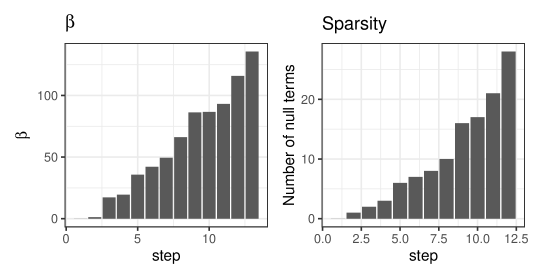
Figure 1: Evolution of $\beta$ and of the sparsity of the solution during the path following algorithm.

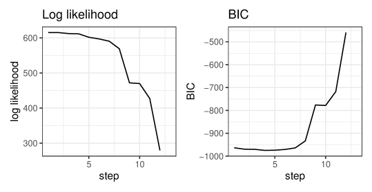
Figure 2: Evolution of the log likelihood and of the BIC of the solution during the path following algorithm.

To evaluate the interest of the path following algorithm on this simple example, we compare four different approaches:

1. our proposed path following Algorithm 3;

2. directly applying the EM Algorithm 2 using the $\beta$s computed by the path, restarting each time the algorithm from the dense initial configuration ($\beta=0$) used by the path following algorithm;

3. directly applying the EM Algorithm 2 using the $\beta$s computed by the path, starting from 10 random initial configurations for each $\beta$;

4. directly applying the EM Algorithm 2 using a regular grid of 50 values for $\beta$ between 0 and the maximum value obtained by the path following algorithm, restarting each time the algorithm from the dense initial configuration ($\beta=0$).

Solution 2 generates exactly the same estimates as the ones obtained by the path following algorithm but in a longer running time (25% more iterations of the EM algorithm).

Solution 3 generates also identical results as the ones obtained by the path following algorithm. However, we used obviously roughly ten times more computational resources and in addition a large number of the initial configurations did not allow the EM algorithm to converge for larger values of $\beta$, as seen on Figure 3.

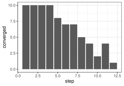
Figure 3: Number of converging EM runs (among 10) in solution 3 as a function of $\beta$ (represented here by the step in the path following algorithm).

Notice finally that the values of $\beta$ are quite unpredictable. Without the path following strategy, we would have had to study the effect of $\beta$s sampled from an arbitrary grid of values, as tested in solution 4. Results are presented on Figures 4 and 5. They show an identical behavior of the grid based search and of the path following algorithm in terms of likelihood and BIC. Some sparsity levels might be missed during the path following (compare Figure 4 and Figure 1), but this is easily fixable by testing some additional values for $\beta$ inside intervals where the jump in sparsity is large.

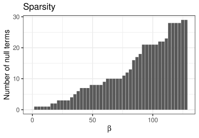
Figure 4: Sparsity of the solution as a function of $\beta$.

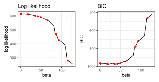
Figure 5: Log likelihood and of the BIC of the solution as a function of $\beta$. The red dots are the configurations obtained by the path following algorithm.

In summary, the path following algorithm provides efficiently a good sampling of the values of $\beta$ that have a significant effect on the sparsity of the solution. If finer grain analysis is needed, one can sample the intervals between values on the path that show a large modification in the sparsity of the solution.

4.3 Simulation study

In this section, we study in a more systematic way the behavior of the proposed methodology. Our goal is to evaluate the computational burden of testing several $\beta$s via the path following strategy (Section 4.3.1), to confirm and complement previous results about model selection with information criteria (Section 4.3.2), to study to what extent those criteria can be used to select an optimal $\beta$ (Section 4.3.3) and finally to assess the difficulty of recovering a planted sparse structure (Section 4.3.4).

The study is based on the $d=100$ dimensional case, with $K^{*}=4$ components and for two degrees of overlapping between the components (2.5 % and 5 %), three level of sparsity in the directional means ( 5 %, 10 % and 15 %) and two data size (200 and 1000 observations, respectively). Notice that while the directional means are sparse, this is not the case of the observations themselves unless the $\boldsymbol{\kappa}$s are set to significantly larger values than the ones we use. We report here only the results obtained for component specific values of $\boldsymbol{\kappa}$ as the ones obtained with a shared $\kappa$ do not depart significantly from them in this setting.

We report statistics obtained by generating 100 data sets for each of the configurations under consideration. In each run, the model is obtained by running the EM algorithm from ten random initial configurations (see B) and by keeping the best final configuration according to the (penalized) likelihood. The path following algorithm is started from this best configuration and is parameterised to ensure a minimum relative increase of $10^{-3}$ between two consecutive values of $\beta$.

4.3.1 Path characteristics and computational burden

The behavior of the path following algorithm is summarized by Figure 7 which shows the distribution of the number of steps taken on the path as well as the distribution of the total number of iterations of the EM algorithm. Compared to the dense case (i.e. to the initialisation of the algorithm) represented on Figure 6, following the path increases significantly the computational burden. However, the increase is far less important that what could be expected from the number of different values of $\beta$ considered during the path exploration. Indeed, the median number of EM iterations needed to obtain an initial dense configuration is larger than $500$ (for $K\geq 2$), while it is smaller than $10000$ for the subsequent path exploration. This 20 times ratio, is significantly smaller than the median number of steps (at least $150$ for $K\geq 2$). In other words, restarting from the previous configuration when $\beta$ is increased is very efficient: in general the new stable configuration is obtained using a small number of iterations of the EM, significantly less than the ones needed to obtain the first dense model.

The results shown here for $N=200$ observations are representative of the results obtained with more observations. The number of iterations tend to grow for larger $K$ when $n$ increases, but that does not change significantly the number of steps on the path or the ratio between the number of EM iterations in the dense case and on the path.

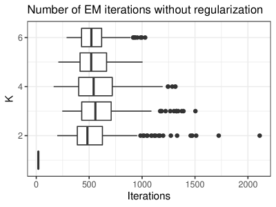
Figure 6: Distributions of the number of EM iterations needed to obtain the first model with $\beta=0$ over 600 data sets with $d=100$ and $N=200$, as a function of $K$, the number of components. The figure aggregates results for all values of the separation and the sparsity.

Figure 7: Distributions of the number of steps (a.k.a. values of $\beta$) and of the total number of EM iterations over 600 data sets with $d=100$ and $N=200$, as a function of $K$, the number of components. The figures aggregate results for all values of the separation and the sparsity.

In summary, the simulation confirms the results obtained in Section 4.2: the computational burden of estimating several models for different values of $\beta$ is large but the path following strategy helps mitigating this cost.

4.3.2 Model selection: number of components

As explained in Section 3.4, previous studies on mixtures of vMF have been somewhat inconclusive about the ability of information criteria to the select the number of components of the mixture. We confirm the complex behavior of the two main criteria (AIC and BIC) in this section.

For each of the 100 replications, we apply the proposed methodology : we keep the original dense model as a reference. Then we select along the $\beta$ path the best model according to each of the information criterion presented in Section 3.4. Finally, we report the number of components selected in this two cases (dense versus sparse) by minimizing the information criteria. Notice that in the dense case, we have a single model evaluated by multiple criteria, while in the sparse case, each criterion selects a different model on the path.

Figures 8 and 9 show the results of this approach in the dense case and in the sparse one (for AIC and BIC), with $N=200$ observations. As the sparsification reduces the number of effective parameters without reducing too much the likelihood, it favors models with more components. In this setting, this proves beneficial for the BIC but drives already the AIC in its overfitting regime.

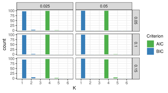
Figure 8: Dense case: number of times each $K$ is selected as the best configuration by AIC or BIC for $\mathbf{N=200}$ observations and $\beta=0$, across overlapping values (in column) and directional mean sparsity (in row).

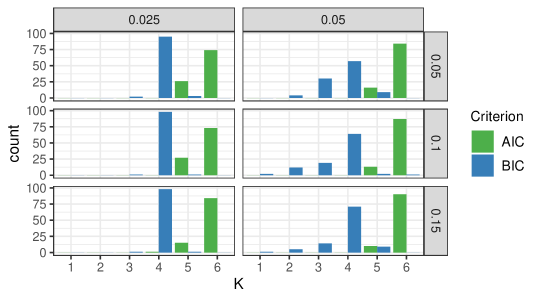
Figure 9: Sparse case: number of times each $K$ is selected as the best configuration by AIC or BIC for $\mathbf{N=200}$ observations for the optimal $\beta$ selected by each criterion, across overlapping values (in column) and directional mean sparsity (in row).

Unfortunately, this overfitting behavior of AIC manifests even more in the simpler case with $N=1000$ observations (see Figures 10 and 11), while BIC on the contrary is able to recover the true number of components, with and without sparsity enforcement.

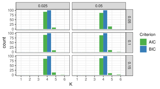
Figure 10: Dense case: number of times each $K$ is selected as the best configuration by AIC or BIC for $\mathbf{N=1000}$ observations and $\beta=0$, across overlapping values (in column) and directional mean sparsity (in row).

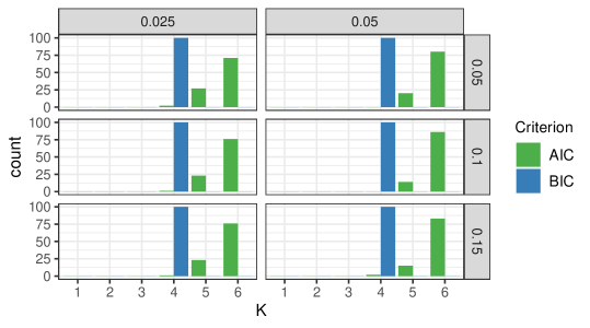
Figure 11: Sparse case: number of times each $K$ is selected as the best configuration by AIC or BIC for $\mathbf{N=1000}$ observations for the optimal $\beta$ selected by each criterion, across overlapping values (in column) and directional mean sparsity (in row).

The simulation study tends to favor the BIC, but this is probably an effect of the reasonable ratio between the dimension $d=100$ and the number of observations $N=200$ and $N=1000$. Experiments in Section 5 and 6 will show examples of a less appropriate behavior of the BIC in more adverse setting, when $d$ is large compared to $n$. This confirms previous results summarized in Section 3.4, which tend to show that information criteria can only be use to guide the exploration of the data for this type of mixture models.

We have not included in this section the results obtained for other information criteria recalled in Section 3.4. On simulated data, they perform uniformly worse than the AIC and the BIC in the small number of observations regime ($N=200$ for $d=100$) and roughly identically to the BIC in the large number of observations case ($N=1000$). We investigate their practical relevance on real world data in Section 5 and 6.

4.3.3 Selection on the path

We study now the effect of selecting the best $\beta$ with the BIC or the AIC. We use as performance metric the adjusted rand index (ARI) between the ground truth and the crisp assignments produced by the different models. Figure 12 shows the results for $N=200$ observations. In this case, the BIC tends to over sparsify the directional means compared to the ARI, especially when the $K=4$, the true number of components.

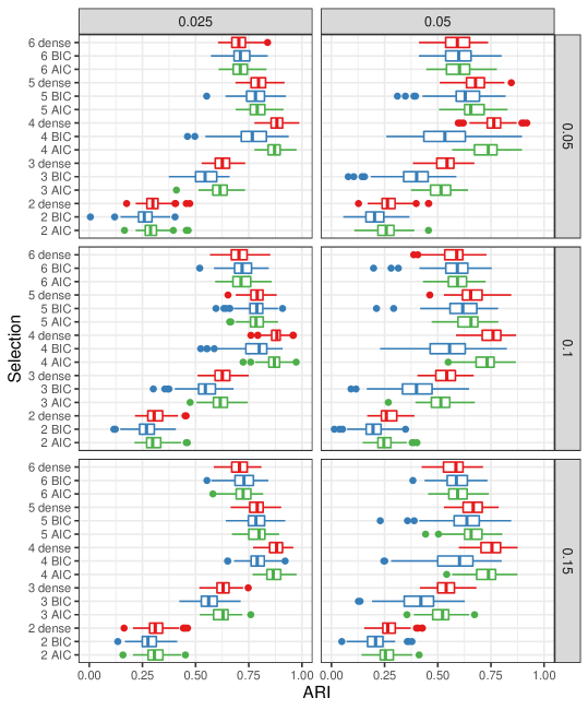
Figure 12: Adjusted rand index distribution for the optimal dense model (in red) and for the optimal sparse models according to the AIC (green) and BIC (blue), as a function of $K$, the number of components, for $\mathbf{N=200}$. Panels are organised based on overlapping (vertically) and on sparsity (horizontally).

The phenomenon is linked to the difficultly of the estimation, as shown on Figure 13 with $N=1000$ observations. When we have more observations, when the true directional means are sparser or when the components overlap less, the ARI drop between BIC and AIC is less pronounced.

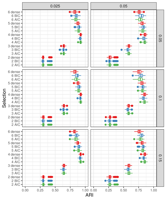
Figure 13: Adjusted rand index distribution for the optimal dense model (in red) and for the optimal sparse models according to the AIC (green) and BIC (blue), as a function of $K$, the number of components, for $\mathbf{N=1000}$. Panels are organised based on overlapping (vertically) and on sparsity (horizontally).

It is also linked to the sparsity achievable given the number of observations, as illustrated by Figures 14 and 15. Indeed with more observations, estimations of the directional mean components are tighter and the non zero ones need a larger value of $\beta$ to be removed. The compromise between sparsity and likelihood is more pronounced toward dense models.

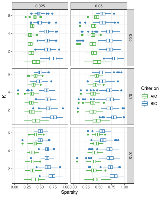
Figure 14: Sparsity achieved by the models selected by AIC and BIC, as a function of $K$, the number of components, for $\mathbf{N=200}$. Panels are organised based on overlapping (vertically) and on sparsity (horizontally).

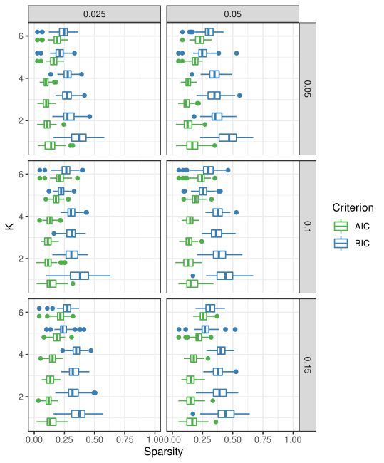
Figure 15: Sparsity achieved by the models selected by AIC and BIC, as a function of $K$, the number of components, for $\mathbf{N=1000}$. Panels are organised based on overlapping (vertically) and on sparsity (horizontally).

4.3.4 Sparse directional mean recovery

Finally, Figure 16 shows the precision and recall of the optimal AIC and BIC models for 100 data sets with $N=1000$ and $d=100$. They are measured by comparing the classification of the coordinates of the directional means into two classes (zero and non zero components) with the true classification induced by sparsifying the directional components during the artificial data generation (notice that this makes sense only when $K=K^{*}$). The low value of the precision confirms the tendency of both criteria to select too sparse representations. On a sufficiently large data set, the BIC as a significantly better recall than the AIC, but with significant loss in precision. Results for smaller data sets tend to be worse in precision and roughly equivalent in recall.

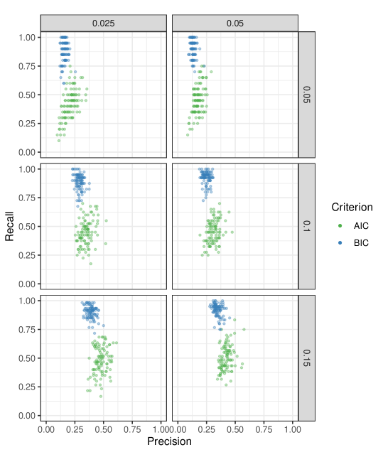
Figure 16: Precision and recall of the zero components of the direction means in the optimal sparse models according to the AIC and BIC for $K=K^{*}=4$ for $N=\mathbf{1000}$ and $d=100$. Panels are organised based on overlapping (vertically) and on sparsity (horizontally).

4.4 Conclusion

In summary, the path following strategy is an efficient way of exploring the sparsification of the solutions. In the low number of observations regime, the use of regularisation enables to select an optimal number of components using the BIC. However in this regime, it also tends to select too sparse directional means compared to the true parameters. Due to the large number of parameters and the high dimension of the data under consideration, this is not surprising, but the experiments show that care should be exercised when using this type of model (regularized or not). The information criteria offer only some general hints for the selection of the best models. In an data exploration point of view, this means that one should consider a collection of models obtained by applying the proposed procedure with different choice of information criterion. The sparsity of directional means is also to be consider with caution.

5 Comparison with reference models

In this section, we compare our model to two reference models designed for directional data, the spherical k-means algorithm [14] and a model based co-clustering algorithm, dbmovMFs, proposed in [30].

We describe briefly the reference models in Section 5.1. Section 5.2 compares the models on the artificial data introduced in Section 4.3, while Section 5.3 compares them on the popular benchmark CSTR.

5.1 Reference models

5.1.1 Spherical k-means (Sk-means)

The spherical k-means algorithm (Sk-means), originally proposed in [14], is a simple adaptation of the k-means algorithm to the cosine dissimilarity. Let us a consider a collection of $N$ observations $\boldsymbol{X}=(\boldsymbol{x}_{i})_{1\leq i\leq N}$ on the hypersphere $\mathbb{S}^{d-1}$. Given a number of clusters $K$, Sk-means tries to find a set of $K$ prototypes $(\boldsymbol{\mu}_{k})_{1\leq k\leq K}$ in $\mathbb{S}^{d-1}$ and a clustering/membership $\boldsymbol{Z}=(z_{i})_{1\leq i\leq N}$, that assigns $\boldsymbol{x}_{i}$ to cluster $z_{i}\in\{1,\ldots,K\}$ such that the coherence

$$\mathcal{Q}((\boldsymbol{\mu}_{k})_{1\leq k\leq K},(z_{i})_{1\leq i\leq N})=\sum_{i=1}^{N}\boldsymbol{\mu}_{k_{i}}^{T}\boldsymbol{x}_{i}$$ (40)

is maximal.

Several methods have been proposed to maximize the coherence (see e.g. [19]). The original method proposed in [14] is Lloyd-Forgy style fixed-point algorithm which iterates between determining optimal memberships for fixed prototypes, and computing optimal prototypes for fixed memberships. In particular the prototypes are the normalized average of the points assigned to their cluster. We used this method in the following experiences (as implemented in the R package skmeans [19]). Apart from the number of clusters $K$, the spherical k-means algorithm has no meta-parameter.

5.1.2 Diagonal Block vMF mixture model (dbmovMFs)

The diagonal block vMF mixture model (dbmovMFs) was proposed in [30]. It can be seen as a constrained version of the classical mixture of vMF distribution. The key idea is to enforce on the directional means a block structure that mimics the one used in co-clustering algorithms. Technically, this is done by introducing a crisp clustering on the dimensions/columns, represented by a crisp assignment matrix $\boldsymbol{W}=(w_{jk})_{1\leq j\leq d,1\leq k\leq K}$, where $w_{jk}=1$ if dimension $j$ is assigned to cluster $k$ and 0 if not (notice that there are as many column clusters as there are components in the mixture).

The directional means are strongly constrained to a diagonal structure, that is

$$\mu_{kj}=w_{jk}\mu_{k},$$ (41)

where $\mu_{k}$ is real number. Thus $\boldsymbol{\mu}_{k}$ has a zero coordinate on all the dimensions that are not assigned to dimension cluster $k$, and a fixed value $\mu_{k}$ on dimensions that are in this cluster. As a consequence, the complete data likelihood as the following form

$$\prod_{i=1}^{N}\prod_{k=1}^{K}\left(\alpha_{k}c_{d}(\kappa_{k})\times\prod_{j=1}^{d}(\exp^{\kappa_{k}\mu_{k}\boldsymbol{x}_{ij}})^{w_{jk}}\right)^{z_{ik}}.$$ (42)

This complete data likelihood is used as the basis of a EM algorithm described in [30]. The algorithm has some common aspect to the one proposed in [2] but also include a specific phase of column cluster update. We use the authors implementation. Notice that the authors proposed several variants of the EM algorithm, but also showed in [30] that the best results are obtained by the classical EM. Therefore we use it in all our experiments. Apart from the number of components $K$, dbmovMFs has no meta-parameter.

5.2 Simulated data

We compare in this section our model to Sk-means and dbmovMFs on the simulated data used in Section 4.3. For each configuration (data size, sparsity and separation), we run Sk-means and dbmovMFs in a similar way as we applied our model: both algorithms are initialized randomly 10 times and the best model is kept according to its specific quality metric (largest coherence for the Sk-means and largest likelihood for dbmovMFs). The random initialisation is similar to the one described in algorithm 4 (random directional means selected from the data set followed by an initial crisp clustering).

DbmovMFs performs extremely poorly on the simulated data, mainly because the sparsity constraints associated to the diagonal block structure are too restrictive. In fact, the EM algorithm fails to converge for a significant part of the initialisation, especially for higher values of $K$: some of the components of the mixture become empty. Notice that this never happens for Sk-means or for our algorithm. Figure 17 illustrates the phenomenon by displaying for each $K$ and each setting, the ratio between the number of converging runs of dbmovMFs and the total of attempted runs. The results are reported for $N=200$ observations but they are even worse for $N=1000$.

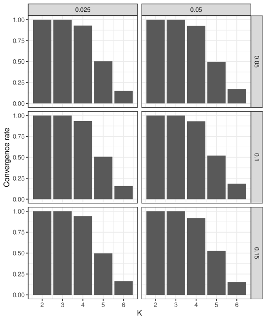
Figure 17: Convergence rates for dbmovMFs for $N=\mathbf{200}$ and $d=100$. Panels are organised based on overlapping (vertically) and on sparsity (horizontally).

In terms of recovering the ground truth as measured by the ARI, both Sk-means and dbmovMFs performances are generally below than the dense solution obtained by our methodology, as shown on Figures 18 and 19. DbmovMFs performs extremely poorly and is unable to recover the planted structure. Spherical k-means results are identical to those of our approach for $N=1000$ and $K=4$. In other configurations (a smaller data set or a mispecification of the number of clusters) that are always inferior, excepted in the particular case of $K=2$.

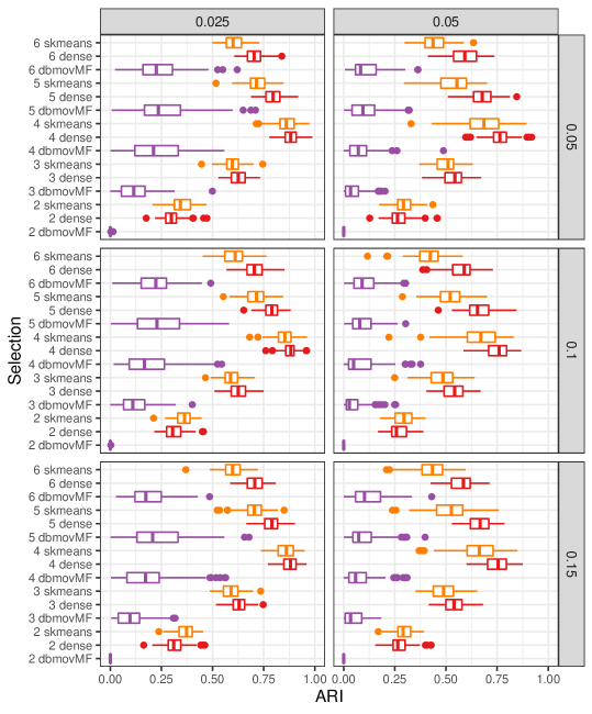
Figure 18: Adjusted rand index distribution for the optimal dense model (in red), for the spherical k-means algorithm (in orange) and for dbmovMFs (in purple), as a function of $K$, the number of components, for $\mathbf{N=200}$. Panels are organised based on overlapping (vertically) and on sparsity (horizontally).

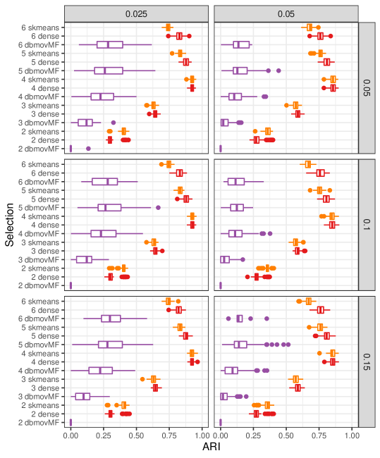
Figure 19: Adjusted rand index distribution for the optimal dense model (in red), for the spherical k-means algorithm (in orange) and for dbmovMFs (in purple), as a function of $K$, the number of components, for $\mathbf{N=1000}$. Panels are organised based on overlapping (vertically) and on sparsity (horizontally).

Notice that the setting is very favorable for Sk-means as the clusters are balanced and use quite similar concentration values $\kappa_{k}$. As pointed out in [30], the performances of Sk-means tend to deteriorate when the true clusters are unbalanced. We have confirmed this behavior by generating another collection of artificial data exactly as in Section 4.3 but with

$$\boldsymbol{\alpha}=\left(\frac{1}{2},\frac{1}{4},\frac{1}{8},\frac{1}{8}\right).$$

Results are provided in Figure 20 the case of $N=1000$ observations. The proposed model recovers the true clustering uniformly better than the Sk-means (the results for $N=200$, omitted, show a larger separation between the methods).

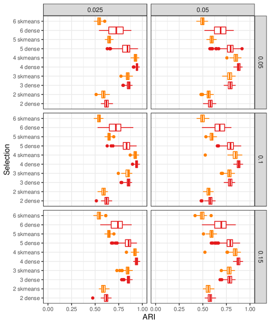
Figure 20: Unbalanced clusters: adjusted rand index distribution for the optimal dense model (in red) and for the spherical k-means algorithm (in orange), as a function of $K$, the number of components, for $\mathbf{N=1000}$. Panels are organised based on overlapping (vertically) and on sparsity (horizontally).

In conclusion, experiments on artificial data show, as expected, that the patterns generated by a mixture of vMF distributions are difficult to recover for Sk-means and nearly impossible to recover for dbmovMFs. The spherical k-means works reasonably well when the data set contains enough observations and when the clusters are balanced, but is outperformed by our approach most of the time. The block structure imposed by dbmovMFs is too strong for it to deal with data with limited sparsity.

5.3 Computer Science Technical Reports (CSTR)

The CSTR data set, proposed in [23], is a good example of a rather high dimensional but small data set with $N=475$ examples in dimension $d=1000$. It has been produced from a selection of 475 abstracts of technical reports published by the Department of Computer Science at the University of Rochester between 1991 and 2002. The reports are represented on an undisclosed dictionary of 1000 words, with a binary encoding (a word is present or not in an abstract). Based on the research areas developed by the CS department at the time of the collection, the abstracts are grouped in $K=4$ classes (Natural Language Processing, Robotics/Vision, Systems, and Theory).

We use this real world data set to compare our approach to Sk-means and dbmovMFs.

5.3.1 Experimental protocol

While CSTR has been used frequently as a benchmark, some care must be exercised in doing so. Indeed the classes of the CSTR data set are not clusters as shown by a simple experiment: using as the initial partition the true classes, an application of the standard spherical k-means algorithm [19] leads to a different partition after convergence. The adjusted rand index (ARI) between the two partitions is of $0.835$. As shown on the confusion matrix between the two partitions (see Table 2), two of the classes are somewhat difficult to recover from a clustering point of view.

	1	2	3	4
1	71	26	3	1
2	0	70	1	0
3	0	1	176	1
4	0	2	5	118

Table 2: Confusion matrix between the classes of the CSTR data set (in row) and the classes obtained by the spherical k-means (in column).

The behavior of the mixture of vMF distributions on CSTR is similar to the one of the spherical k-means. Using the same initialisation, we obtain after convergence an ARI of $0.818$ with component specific $\kappa$s and of $0.837$ with a common $\kappa$. The confusions matrices (omitted) are almost identical to the spherical k-means one. As a consequence, an ARI around $0.84$ should be considered as the maximum a method can reach on this data set. Higher results could be only a matter of chance or obtained with a notion of cluster that is more aligned with the ground truth classes.

Another difficulty is the small size of the data set compared to its number of features. This increases the variance of the estimates provided by any algorithm and as a consequence, the final clustering obtained by different methods from a random initialization tend to be much more dependent on this initial configuration than in the case of a simpler data set (as e.g. in the artificial data experiments reported above). To provide meaningful results, we proceed as follows. For each algorithm, we use a common set of 50 random initial configurations (obtained with algorithm 4): this ensure that the algorithms are used under exactly the same testing conditions. After convergence of a given algorithm, we keep the best configuration in terms of the quality criterion of this algorithm (e.g. the likelihood for mixture models) and report the ARI of the corresponding clustering. We repeat this procedure 50 times (thus considering 250 random initial configurations) to assess the variability of the results.

5.3.2 Results for the dense models: ARI

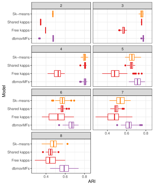
Figure 21: Adjusted Rand Index between the CSTR classes and the clusters obtained by Sk-means, mixture of vMF distributions with a common $\kappa$ parameter (shared kappa) and mixture of vMF distributions with component specific $\kappa$s (free kappa), and dbmovMFs for different values of $K$.

Figure 21 and Table 3 summarize the results obtained by the spherical k-means, dbmovMFs and the two dense variants of the mixtures of vMF. The mixture with component specific concentration parameters has by far the largest variability and the worst results. The adverse effects of a too high value for the concentration parameter on real world data was already established in e.g. [20, 30]. As far as we know, the very strong sensitivity of the results to the initial configuration is a new result (as far as we know). Both issues are solved by using a shared concentration parameter. The variability of the results is then smaller than the one observed for the spherical k-means and on the optimal configuration with $K=4$, the results are roughly identical. In particular, a paired t-test does not show significant differences at a 1% level between the spherical k-means and the shared $\kappa$ mixture of vMF for $K\in\{3,4,5,6\}$.

	SK-means		Shared $\kappa$		Free $\kappa$		dbmovMFs
K	mean	sd	mean	sd	mean	sd	mean	sd
2	0.471	$4.52\,10^{-3}$	0.344	$2.95\,10^{-3}$	0.395	$3.28\,10^{-4}$	0.442	$6.28\,10^{-2}$
3	0.757	$1.31\,10^{-2}$	0.756	$3.83\,10^{-3}$	0.567	$1.89\,10^{-2}$	0.772	$7.35\,10^{-3}$
4	0.802	$1.77\,10^{-2}$	0.804	$1.22\,10^{-2}$	0.519	$4.48\,10^{-2}$	0.803	$1.72\,10^{-2}$
5	0.659	$4.05\,10^{-2}$	0.650	$2.11\,10^{-2}$	0.497	$8.78\,10^{-2}$	0.716	$4.06\,10^{-2}$
6	0.572	$4.59\,10^{-2}$	0.569	$2.24\,10^{-2}$	0.520	$9.51\,10^{-2}$	0.663	$4.15\,10^{-2}$
7	0.535	$5.21\,10^{-2}$	0.493	$2.82\,10^{-2}$	0.463	$8.28\,10^{-2}$	0.625	$5.18\,10^{-2}$
8	0.481	$4.99\,10^{-2}$	0.448	$3.13\,10^{-2}$	0.441	$7.37\,10^{-2}$	0.588	$6.16\,10^{-2}$

Table 3: Adjusted Rand Index between the CSTR classes and the clusters obtained by the models under study.

As shown in [30], the block structure enforced by dbmovMFs is also an efficient way of controlling the adverse effects of the concentration parameters. While the results for $K=4$ are identical to the ones obtained by other methods, dbmovMFs is far more robust to a misspecification of the number of components. Apart for $K=2$ where the spherical k-means provide the best ARI (significant difference at a 1% level), in all other configurations with $K\neq 4$, the ARI obtained by the dbmovMFs is significantly larger than the ones obtained by other methods.

DbmovMFs appears therefore to provide a more robust solution than dense models such as classical mixtures of vMF distributions and than spherical k-means, thanks to its good behavior under mispecification of the number of clusters. Notice however that it had extremely poor results on denser data, as shown on the simulated data.

5.3.3 Results for the dense models: model selection

Figures 22 and 23 display the behavior of the model selection criteria for the shared $\kappa$ mixture of vMF and for dbmovMFs. They show quite different behaviors. For the vMF distribution strongly penalized criteria should be used to recover the best models, while on the contrary, the small number of parameters of the co-clustering approach leads to a better behavior of the AIC.

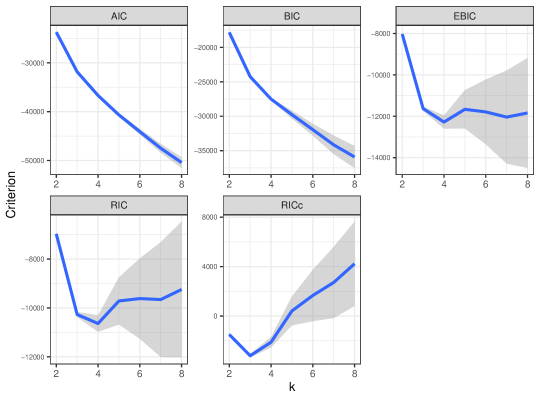
Figure 22: Model selection criteria for the mixture of vMF distributions with a common $\kappa$ parameter: the blue curve is the mean value, while the grey envelop displays a 2 standard deviation tube around it.

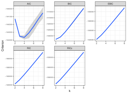
Figure 23: Model selection criteria for dbmovMFs: the blue curve is the mean value, while the grey envelop displays a 2 standard deviation tube around it.

Those quite different behaviors do not give a major advantage of one algorithm over the other on the CSTR data set. We will see in Section 6 that dbmovMFs is probably overpenalized even by the AIC for more complex data sets and that vMF mixtures are probably underpenalized even by e.g. the RIC. This confirms the limitations of information criterion for this type of unsupervised high dimensional models. As a consequence we argue that they should be used to guide the exploration rather than as a proof of existence of a specific number of clusters.

5.3.4 Sparse models

On a second step, we compute the $\beta$ path for each of the 50 replications of our procedure, starting each time from the best initialization obtained from the 50 random initial configurations. We restrict ourselves to the shared $\kappa$ model. Figure 24 and Table 4 summarize the results. In terms of sparse model selection, AIC, BIC and EBIC provide good compromises between the ARI and the sparsity. Both RIC and RICs select a too sparse model.

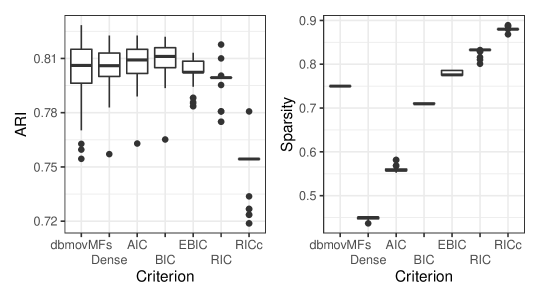
Figure 24: Adjusted rand index and sparsity for the models selected on the $\beta$ path using the different model complexity criteria. The “dense” configuration corresponds to the solution obtained without regularization. DbmovMFs results are given for reference.

Criterion/model	mean	sd
dbmovMFs	0.803	$1.723\times 10^{-2}$
Dense	0.804	$1.217\times 10^{-2}$
AIC	0.807	$1.083\times 10^{-2}$
BIC	0.808	$9.483\times 10^{-3}$
EBIC	0.803	$7.687\times 10^{-3}$
RIC	0.797	$7.991\times 10^{-3}$
RICc	0.750	$1.248\times 10^{-2}$

Table 4: Adjusted Rand Index between the CSTR classes and the clusters obtained by the sparse models under study.

A very important point is that none of the criteria is able to provide an all-in-one selection. Indeed, as shown on Figure 22, the number of components should be selected with EBIC or RIC (and possibly with RICc), as both AIC and BIC are monotonically decreasing with the number of components. However, if we compute the $\beta$ path for different number of components and keep as the selected model the ones that minimize each criteria, this behavior applies to all criteria. In other words, the regularization is compensating for the increased number of components. Thus one should first select the number of components based on EBIC or RIC, and then select the sparsity level with BIC or EBIC, keeping the number of components fixed. Both sparse models selected by AIC and BIC are significantly better than the dense model (according to a paired t-test at a 1% level). The BIC results are only significantly better than the dbmovMFs results at a 10% level.

In summary, using the proposed approach allows to reach similar performances as dbmovMFs without enforcing a specific sparsity structure. On the contrary, the sparsity is learned from the data without performance loss.

5.3.5 Data exploration

We use in this section the visualisation method described in Section 3.5 in order to display the sparsity structure discovered by the proposed method (we restrict the illustration to $K=4$).

Figure 25 represents the block structure obtained by dbmovMFs algorithm of [30]. As expected, this is a very crude model that does favor sparsity over revealing shared coordinates and finer structure. For the point of view of dbmovMFs, the reports are described by a collection of specific vocabulary with for instance the largest cluster (top row) using the largest “private” vocabulary (top right rectangle).

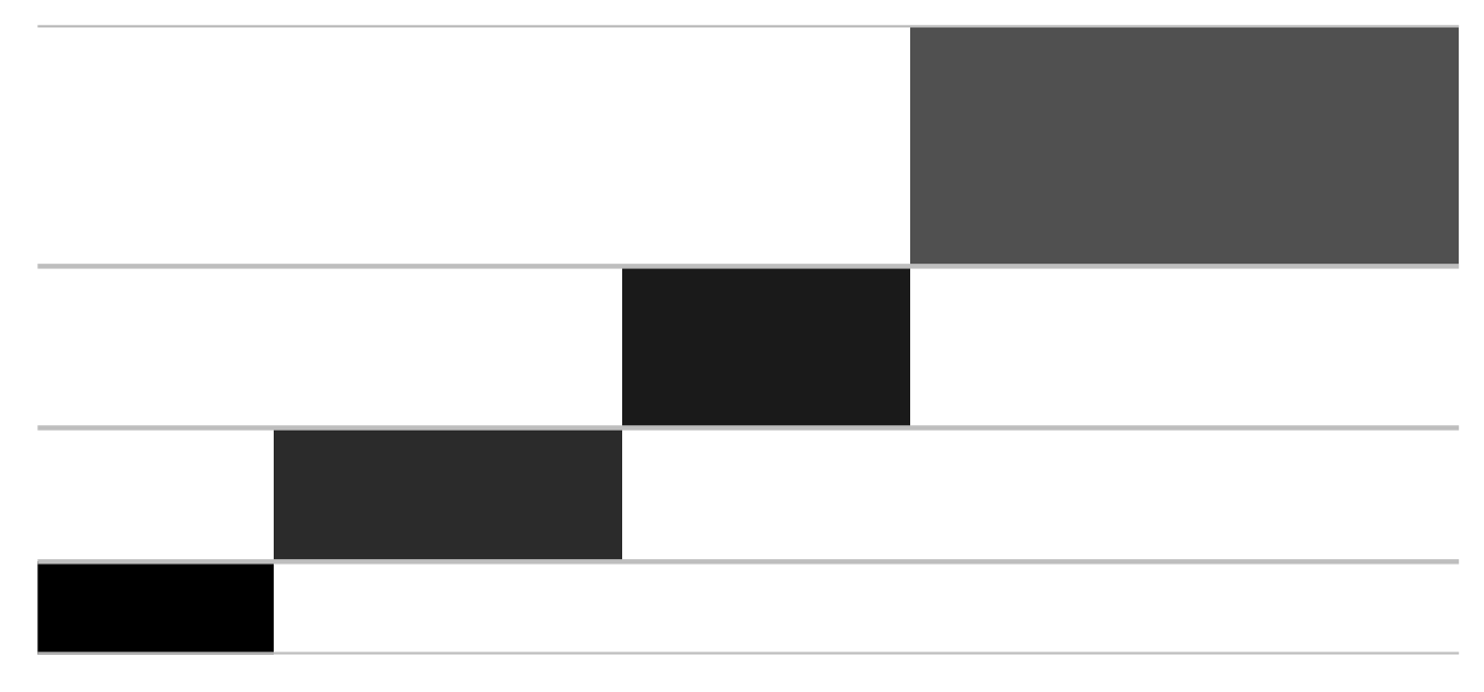
Figure 25: Representation of the directional means obtained by dbmovMFs on the CSTR data set.

Figure 26 represents the full data set using the same ordering: it shows clearly that the coclustering provides only a crude approximation of actual structure of the data. For instance, the smallest cluster (bottom row of Figure 26) uses all the words/dimensions that should be specific to the other clusters. Dark vertical lines on the figure show that some words/dimensions are common to all clusters. The diagonal structure enforced by dbmovMFs is very useful to bring stability to the model estimation and to recover the overall clustering structure, but it appears to be to simplistic to capture the true sparsity structure.

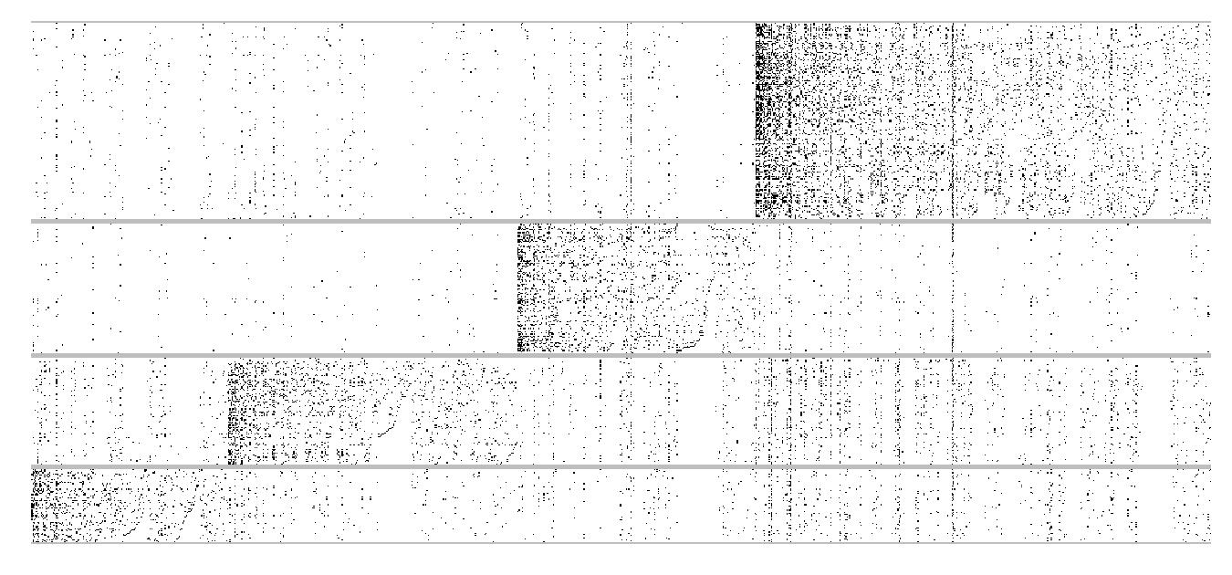
Figure 26: Representation of the CSTR data set reorganized as the directional means obtained by dbmovMFs.

Figure 27 shows the structure of the directional means for the mixture of vMF obtained without regularization. As shown be the colors, there are four blocks of dimension: from the block of dimensions/words common to all texts on the left to the block of cluster specific words. The two intermediate blocks corresponds respectively to vocabulary shared by 3 clusters and 2 clusters. This representation confirms that there are indeed specific coordinates but it shows that the clusters share dimensions in a large proportion, confirming that dbmovMFs hides most of the structure.

Figure 27: Representation of the directional means obtained by the mixture of vMF with shared $\kappa$ on the CSTR data set.

Figure 28 represents the directional means obtained by selecting with the BIC the best sparse model along the $\beta$ path. The result is a compromise between the strictly diagonal structure obtained by dbmovMFs and the denser solution obtained without regularisation. It isolate better the specific dimensions/vocabulary while keeping a smaller subset of shared dimensions. Notice also that we have now a fifth block of dimensions: those can be considered as noise dimensions as the corresponding coordinates are uniformly null in the directional means.

This is confirmed by Figure 29 that shows the data set reorder in the same way as the directional means according to the sparse mixture of vMF. The reordering reveals in a clearer way the underlying structure of the data. In particular the pink area which corresponds to the diagonal substructure with “private” vocabulary is far less noisy than in the case of dbmovMFs.

Figure 28: Representation of the directional means obtained by the mixture of vMF with shared $\kappa$ and regularisation on the CSTR data set.

Figure 29: Representation of the CSTR data set reorganized as the directional means obtained by the mixture of vMF with shared $\kappa$ and regularisation.

5.4 Conclusion

The comparisons conducted in the Section have shown several important results. On relatively dense data, the spherical k-means and the mixture of vMF distribution behave in a similar way. The mixture model is more flexible in terms of unbalanced between the clusters and recovers them with less data than the spherical k-means as a consequence of modeling explicitly the concentration of each cluster. On the contrary, the strong constraints of dbmovMFs prevents it from inferring a correct structure for relatively dense data.

On sparse data, dbmovMFs tends to be more stable and more robust against mispecification than both spherical k-means and vMF distribution mixtures. The mixture model with component specific concentration parameters should be avoided when the number of observations is not significantly larger than the dimensions. A shared concentration parameter is sufficient to bring stability to the mixture model, but mispecification remains a problem. Overall, the best results are obtained by the sparse mixture proposed in the paper. In terms of recovering the clustering structure it obtains results roughly identical to the ones obtained by the other models, but it reveals patterns in the directional means that are more consistent with the data than the diagonal structure imposed by dbmovMFs.

6 Exploratory analysis on 8-K reports 2015 - 2019 for Wells Fargo

Following [22] and completing the database proposed by [3], we create a dataset which focus on 8-K reports. An 8-K is a report of unscheduled material events or corporate changes at a company that could be of importance to the shareholders or the Securities and Exchange Commission (SEC). Also known as a Form 8K, the report notifies the public of events, including acquisitions, bankruptcy, the resignation of directors, or changes in the fiscal year. We have compiled this dataset, thanks to SEC’s EDGAR tool, for the years 2015 - 2019 on all companies from the Standard and Poors 500.

The corpus contains $37,238$ reports issued by $592$ companies. The texts were pre-processed by applying a classical pipeline:

• removal of non-alphanumeric characters;

• lemmatisation;

• removal of words appearing less than $100$ times and stopwords: we obtain a dictionary of $70223$ distinct roots for the whole corpus.

The number of reports produced over the period varies greatly depending on the company concerned. A preliminary analysis shows that the vocabulary of the texts depends heavily on the company, in particular because of the different sectors of activity but above all depending on the context (economic, social, etc.). We therefore carry out the exploration company by company and in particular for this article to focus on Wells Fargo (WFC) as they published the most during this period.

This company published $672$ reports for the years $2015$ and $2019$ and out of $25$ possible events, only $7$ are represented, with a domination of the event financial statements and exhibits, which tends to show that these reports are mainly about the financial state of the company (see table 5 for event titles and their frequencies). Note that reports can share multiple events. Only $4377$ words (roots) are used in the reports and this dataset is as follow $N=672$ in dimension $d=4377$.

Code	Type	Frequencies
1	Financial Statements and Exhibits	658
2	Results of Operations and Financial Condition	24
3	Amendments to Articles of Incorporation or Bylaws; Change in Fiscal Year	19
4	Departure of Directors or Certain Officers; Election of Directors; Appointment of Certain Officers: Compensatory Arrangements of Certain Officers	27
5	Submission of Matters to a Vote of Security Holders	5
6	Other Events	36
7	Amendments to the Registrant’s Code of Ethics, or Waiver of a Provision of the Code of Ethics	2

Table 5: Wells Fargo Events

In what follows, we will first analyse our dataset with the reference models and then with our own.

6.1 Reference models

As the number of clusters $K$ is unknown in this case, we used different methods depending on the reference models. For dbmovMFs, AIC was used and it selected $K=3$, as seen in Figure 30. Whereas for Sk-means, we used the Calinski-Harabasz index [9] and obtained $K=2$.

Figure 30: Model selection criteria for dbmovMFs concerning the analysis of Wells Fargo: the blue curve is the mean value, while the grey envelop displays a 2 standard deviation tube around it.

Table 6 shows the distribution of reports by cluster obtained by both algorithms. We can note that in both cases, one class is predominant and the second class of Sk-means is dispersed in the three classes of dbmovMFs. Moreover, an ARI of more than $80\%$ shows the similarities between these two clustering.

	Clusters
Algorithms	1	2	3
Sk-means	570	102	-
dbmovMFs	22	53	597

Table 6: Distribution of reports by cluster obtained by dbmovMFs selectionned by AIC and Sk-means with the Calinski-Harabasz index.

For these reasons, we will now focus on the analysis of the clustering obtained with dbmovMFs.

Figure 31 represents the block structure obtained by dbmovMFs. As observed previously, the dbmovMFs solution hides most of the structure and does not facilitate a detailed analysis.

Figure 31: Representation of the directional means obtained by dbmovMFs on the Wells Fargo data set.

Figure 32 shows the distribution of events by cluster. It appears that the $1$ is largely composed by financial reports with events as Financial Statements and Exhibits and Results of Operations and Financial Condition. From Figure 33, we can assert that reports of this class are quarterly reports. Class 2 is mainly concerned by specific events such as Departure of Directors or Certain Officers; Election of Directors; Appointment of Certain Officers: Compensatory Arrangements of Certain Officers or Submission of Matters to a Vote of Security Holders. Figure 33 exhibits that this class appears when the company has had to face a negative context and has wanted to reorganise. Class $3$, consisting mainly of the event Financial Statements and Exhibits, concerns the company’s various financial communications. However, unlike the detailed analysis possible with the mixture of vMF that we develop below, it is very difficult here to see the different aspects of its financial communication and the financial products it issues.

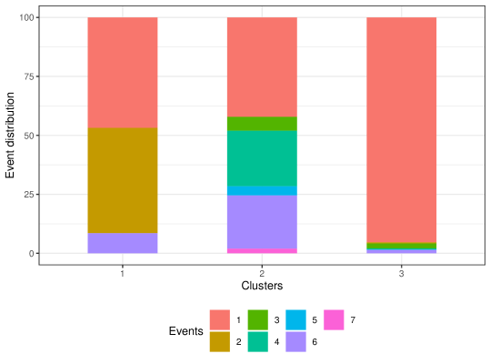
Figure 32: Distribution of events by cluster in the Wells Fargo dataset obtained with dbmovMFs.

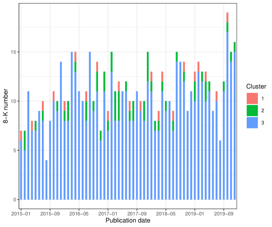
Figure 33: Distribution of the reports’ number per cluster by month in the Wells Fargo dataset obtained with dbmovMFs.

6.2 Mixture of vMF with a common $\kappa$ parameter

To select the number of clusters $K$, we proceed as exposed previously using the mixture of vMF with a common $\kappa$ parameter. As the first step, we select the number of components thanks to the RICc to obtain $K=14$ as shown in Figure 34.

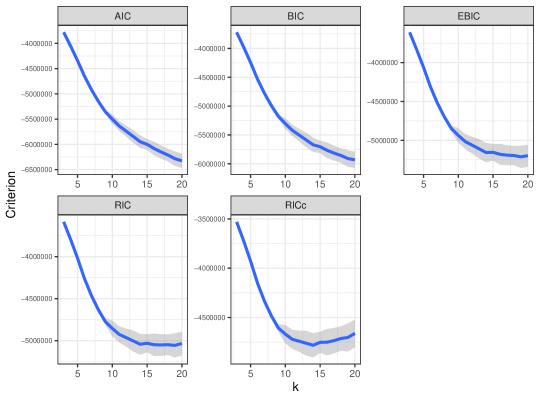
Figure 34: Model selection criteria for the mixture of vMF distributions with a common $\kappa$ parameter concerning the analysis of Wells Fargo: the blue curve is the mean value, while the grey envelop displays a 2 standard deviation tube around it.

In the second step, the sparsity level was selected using the path following strategy with a maximum of $1000$ steps and the minimal relative increase between two values of $\beta$ set to $0.01$. A $\beta$ of $1072.253$ and a sparsity of $82.16\%$ were obtained. Figures 35 represents the directional means. Figure 36 exhibits the data set reorganized as directional means. It reveals in a clearer way the underlying structure of the data.

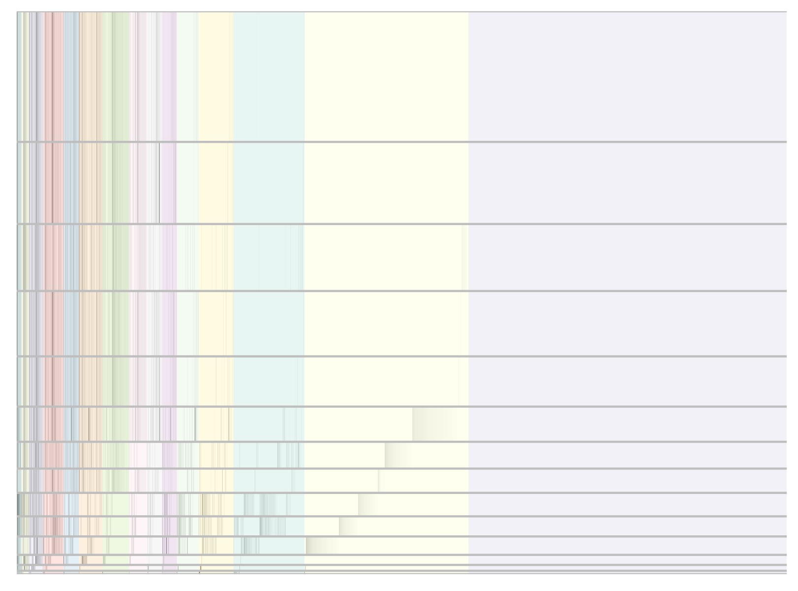
Figure 35: Representation of the directional means obtained by the mixture of vMF with shared $\kappa$ and regularisation on the Wells Fargo data set.

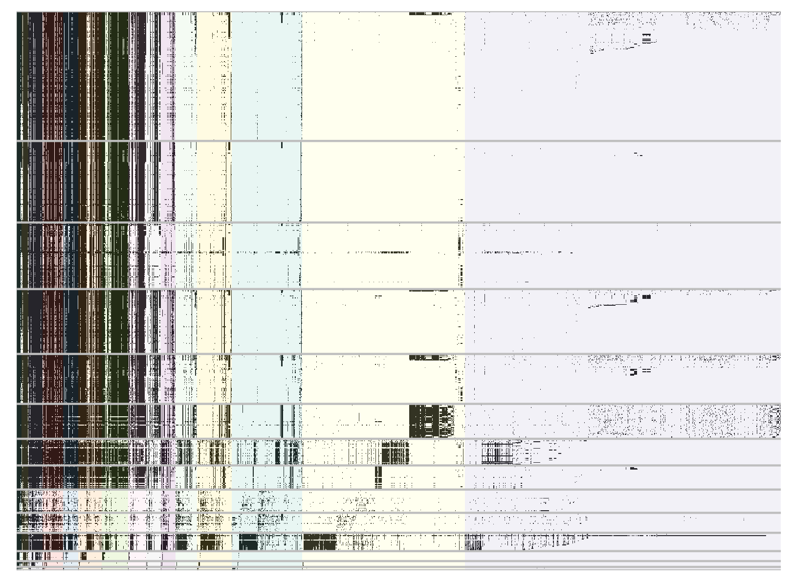
Figure 36: Representation of the Wells Fargo data set reorganized as directional means obtained by the mixture of vMF with shared $\kappa$ and regularisation.

Table 7 shows the distribution of reports by cluster obtained. The result is very different from those obtained previously with ARIs below $9\%$ in comparison to clusterings of dbmovMFs and Sk-means. We can note that cluster $3$ is the biggest one with $156$ reports while clusters $1$ and $4$ are composed of very few of them and must be focused on one topic. Moreover, It appears that class $13$ is identical to class $1$ found by dbmovMFs.

	Clusters
	1	2	3	4	5	6	7	8	9	10	11	12	13	14
Nb. 8-K	4	80	156	7	12	78	32	60	42	98	24	28	22	29

Table 7: Distribution of reports by cluster obtained by the sparse model selectionned by RICc with the path following approach.

For its part, table 8 shows the unique words by cluster and those in common. The latter makes sense in that they contain generic terms in the company’s reports, such as its name or the name of a financial instrument for example. More interesting are the unique words for each cluster as they form coherent subjects. Note the exception for clusters 5 and 10, which share all their representatives’ words with at least another cluster.

For instance, unique words of cluster 1 - abstention, cast, ratify, shareowner - are from the annual meeting lexicon. Figure 39 shows that this cluster is entirely composed of the Submission of Matters to a Vote of Security Holders event which takes place annually as visible in Figure 40. Figure 37 shows an extract of a report from Cluster 1 published by Wells Fargo on 1 May 2015. Words in blue represent the common words between all Clusters and in red, the ones specific to this Cluster.

Cluster	1	2	3	4	5
1	abstention	cast	ratify	shareowner	-
2	continuance	bankrupt	insolvent	receiver	annually
3	vme	monthly	shewchuk	sonia	cqr
4	advisable	convene	nonassessable	-	-
5	-	-	-	-
6	sector	bad	homebuilders	gold	miner
7	untrue	omission	canadian	directive	representation
8	adr	absent	determinable	fluctuation	bloomberg
9	domainitemtype	false	thinterestinshareof	shr	text
10	-	-	-	-	-
11	defendant	chair	bonus	rsrs	hear
12	mack	banker	unauthorized	parent	controller
13	portfolio	revenue	offs	sep	jun
14	gics	spin	otc	bulletin	antidilution
commun	security	company	any	well	fargo

Table 8: Unique words for each cluster obtained by the sparse model selectionned by RICc with the path following approach. The row commun shows words shared by all clusters.

Event :

Submission of Matters to a Vote of Security Holders.;

Text :

[…] wells fargo company held its annual meeting of stockholders on april 28, 2015. at the meeting, stockholders elected all 16 of the directors nominated by the board of directors as each director received a greater number of votes cast for his or her election than votes cast […] ratify the appointment of kpmg llp as independent registered public accounting firm for 2015 […].

Figure 37: Example of a Cluster 1 8-K report published on 1 May 2015. Words show the commun ones between all cluster and words, the ones specific to cluster 1.

If we now look at Cluster 11, which appears randomly over time in Figure 40, it is composed of events Financial Statements and Exhibits, Other Events and especially Departure of Directors or Certain Officers; Election of Directors; Appointment of Certain Officers: Compensatory Arrangements of Certain Officers. This cluster focuses on changes in the board and their possible consequences on the company’s results. Figure 38 shows an extract of a report from Cluster 11 published by Wells Fargo on 12 October 2016 notifying the departure of CEO John Stumpf in the wake of numerous scandals. It is interesting to note that the unique words of this Cluster express this context. First, the word chair refers to a person who sits on the Board of Directors. Second, the term defendant implies legal proceedings. Finally, terms bonus and rsrs mention compensation due to the turnover of board members.

Event :

Departure of Directors or Certain Officers; Election of Directors; Appointment of Certain Officers: Compensatory Arrangements of Certain Officers & Financial Statements and Exhibits.;

Text :

[…] on october 12, 2016, john g. stumpf notified wells fargo company ) of his decision to retire as chairman and chief executive officer and a director of the company, effective immediately. […] elected director elizabeth a. duke as the company s non-executive vice chair. […].

Figure 38: Example of a Cluster 11 8-K report published on 12 October 2016. Words show the commun ones between all cluster and words, the ones specific to cluster 11.

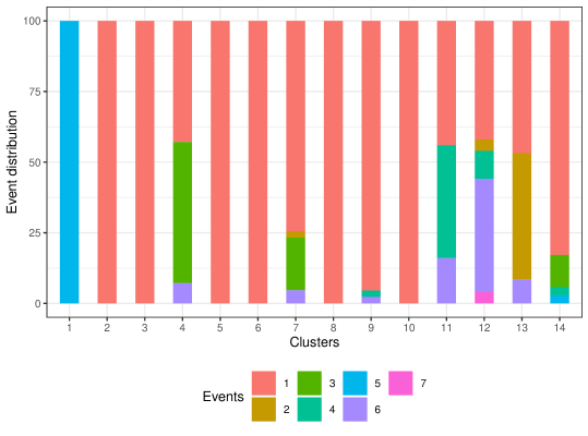
Figure 39: Distribution of events by cluster in the Wells Fargo dataset with the model obtained by the path following approach.

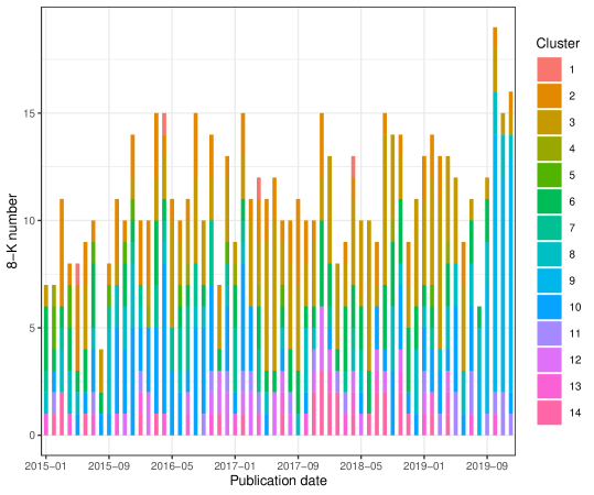
Figure 40: Distribution of the reports’ number per cluster by month in the Wells Fargo dataset with the model obtained by the path following approach.

Let us now focus on clusters that are made up of the same single event type and do not have unique terms such as clusters 5 and 10, as seen in Figure 39. Figure 40 shows that these clusters appear differently over time. Cluster 5 focuses mainly on the period before the resignation of the CEO, i.e. before October 2016, while cluster 10 is found significantly in two periods, i.e. between July 2015 and March 2017 but also between April 2018 and July 2019. These two periods correspond to many legal cases but also to setbacks in business for Wells Fargo. These include high exposure to the fall in oil prices in January 2016 and numerous settlements of fines for fraudulent business practices in April 2018 and concerning the sub-prime crisis in August 2018. An in-depth reading of the texts of these clusters reveals a common subject between them, namely medium-term notes, but of different series and different underlying assets. Cluster 10 is related to medium-term notes, series K, linked to indexes based on Emerging Markets such as the iShares MSCI Emerging Markets ETF or developped market as the MSCI EAFE Index. Cluster 5 is associated to medium-term notes, series N, linked to reference rates. These clusters, therefore, show that the company has issued different types of debt to cope with its context and ensure its financing needs.

Finally, the previous analysis shows the advantages of our method comparing to dbmovMFs for an exploratory analysis. It exhibits the specialisation of each of the clusters which allows an easy understanding of the different events that impact a company over time. Moreover, when they exist, unique words to each cluster give a precise idea of the main subject of said cluster. For their part, shared terms between all clusters provide an overview of the corpus’ subject.

7 Conclusion

In this article, we have proposed to estimate a mixture of von Mises-Fisher distributions using a $l_{1}$ penalized likelihood. This model attempts to learn sparse directional means without enforcing a diagonal structure, contrarily to dbmovMFs. Sparse directional means provide a way to understand the data structure and to interpret the clustering induced by the mixture model.

The maximisation of the penalized likelihood is implemented via expectation-maximization. To avoid estimating parameters from scratch for different trade-offs between the likelihood and the penalty term, we introduced a path following approach that detect automatically important change in the sparsity of the solutions. We showed that selecting the best trade-off can then be done using the BIC. We also confirmed previous results about the difficulty of selecting the number of components of the mixture in the high dimensional case with a relatively low number of observations. Finally, we proposed a pixel oriented visualisation technique to represent sparse directional means and provide a first insight on the structure of the data.

Extensive qualitative and quantitative experiments on differents data sets, including a new dataset of Wells Fargo 8-K reports, demonstrate the practical interest of the proposed model. Indeed, the sparsity of the directional means obtained eases the interpretation of results while achieving similar or better results in terms of ARI.

However, our results also confirm that dbmovMFs remains more stable than a mixture of vMF distributions, essentially as a consequence of its low concentration parameters. As the diagonal structure enforced on the directional means is very strong, the clusters obtained by dbmovMFs remain somewhat vague. As shown in our experiments, the directional means obtained by dbmovMFs are only remotely representative of the true structure of the data. Using a shared concentration parameter, we managed to bring mixtures of vMF distributions on par with dbmovMFs when the model is correctly specified in terms of cluster number. In the future, we will investigate other ways to constrain the concentration parameters in order to improve the stability of our model without compromising the quality of the directional means. A possible solution would be to use a regularisation term on the concentration parameters, but this introduces at least two difficulties. Firstly the maximisation phase will be much more complicated, considering that it would introduce a regularisation term in an already difficult numerical problem (summarized by equation (21)). Secondly, when all the other parameters are held constant, the likelihood increases with increasing values of the concentration parameters. It would therefore be necessary to introduce a way to define an optimal trade-off between regularizing the concentrations and maximizing the likelihood. As the regularisation will have to effect on the number of parameters, information criteria will be of no help in this setting.

Finally, let us mention that the path-following strategy proposed in this work could be easily adapted to other penalized models such as the Gaussian mixture proposed in [26].

Appendix A Derivation of the EM algorithm

We derive in this Section the first order optimality conditions of the M phase of the EM algorithm.

A.1 Stationary point equations associated to the $\kappa_{k}$

The Lagrangian (19) has partial derivatives with respect to $\kappa_{k}$ given by

$$\frac{\partial}{\partial_{\kappa_{k}}}\mathcal{L}(\boldsymbol{\Theta},\zeta,\boldsymbol{\lambda}|\boldsymbol{\Theta}^{(m)})=\sum_{i=1}^{N}\tau^{(m)}_{ik}\left(\frac{c^{\prime}_{d}(\kappa_{k})}{c_{d}(\kappa_{k})}+\boldsymbol{\mu}_{k}^{T}\boldsymbol{x}_{i}\right).$$ (43)

To simplify this expression, we follow [2] and compute

$$c^{\prime}_{d}(\kappa_{k})=\frac{1}{(2\pi)^{s+1}I^{2}_{s}(\kappa_{k})}\left(s\kappa_{k}^{s-1}I_{s}(\kappa_{k})-\kappa_{k}^{s}I^{\prime}_{s}(\kappa_{k})\right),$$ (44)

where $s=\frac{d}{2}-1$ and $I^{\prime}_{s}$ is the derivative of modified Bessel function of the first kind and order s. As recalled in [2], this derivative is such that

$$\kappa_{k}I_{s+1}(\kappa_{k})=\kappa_{k}I^{\prime}_{s}(\kappa_{k})-sI_{s}(\kappa_{k}),$$ (45)

and thus

$$c^{\prime}_{d}(\kappa_{k})=-\frac{\kappa_{k}^{s}I_{s+1}(\kappa_{k})}{(2\pi)^{s+1}I^{2}_{s}(\kappa_{k})},$$ (46)

leading to

$$\frac{c^{\prime}_{d}(\kappa_{k})}{c_{d}(\kappa_{k})}=-\frac{I_{s+1}(\kappa_{k})}{I_{s}(\kappa_{k})}.$$ (47)

Then $\frac{\partial}{\partial_{\kappa_{k}}}\mathcal{L}(\boldsymbol{\Theta},\zeta,\boldsymbol{\lambda}|\boldsymbol{\Theta}^{(m)})=0$ is equivalent to

$$\frac{I_{d/2}(\kappa_{k})}{I_{d/2-1}(\kappa_{k})}=\boldsymbol{\mu}_{k}^{T}\frac{\sum_{i=1}^{n}\tau^{(m)}_{ik}\boldsymbol{x}_{i}}{\sum_{i=1}^{n}\tau^{(m)}_{ik}}.$$ (48)

A.2 Stationary point equations associated to the $\boldsymbol{\mu}_{k}$

For the directional means, we have to consider the sub-gradient of the Lagrangian function. We have

$$\partial_{\mu_{kj}}\mathcal{L}(\boldsymbol{\Theta},\zeta,\boldsymbol{\lambda}|\Theta^{(m)})=\kappa_{k}\left(\sum_{i=1}^{n}\tau^{(m)}_{ik}x_{ij}\right)-2\lambda_{k}\mu_{kj}-\beta\partial_{\mu_{kj}}\lvert\mu_{kj}\rvert.$$ (49)

Using the well known property of the sub-gradient of the absolute value, we obtain

$$\partial_{\mu_{kj}}\mathcal{L}(\boldsymbol{\Theta},\zeta,\boldsymbol{\lambda}|\Theta^{(m)})=\left\{\begin{array}[]{ll}\{\kappa_{k}r^{(m)}_{kj}-2\lambda_{k}\mu_{kj}+\beta\}&\text{when }\mu_{kj}<0,\\ \{\kappa_{k}r^{(m)}_{kj}-\epsilon\beta|\epsilon\in\left[-1;1\right]\}&\text{when }\mu_{kj}=0,\\ \{\kappa_{k}r^{(m)}_{kj}-2\lambda_{k}\mu_{kj}-\beta\}&\text{when }\mu_{kj}>0,\end{array}\right.$$ (53)

where

$$\boldsymbol{r}^{(m)}_{k}=\sum_{i}\tau^{(m)}_{ik}\boldsymbol{x}_{i}.$$ (54)

The first-order optimality condition is $0\in\partial_{\mu_{kj}}\mathcal{L}(\boldsymbol{\Theta},\zeta,\boldsymbol{\lambda}|\Theta^{(m)})$, which leads to the following analysis.

If we look for a positive solution $\mu_{kj}>0$, the optimality condition is fulfilled when

$$\mu_{kj}=\frac{\kappa_{k}r^{(m)}_{kj}-\beta}{2\lambda_{k}}.$$ (55)

This solution is compatible with $\mu_{kj}>0$ if $\kappa_{k}r^{(m)}_{kj}-\beta>0$, that is when $r^{(m)}_{kj}>\frac{\beta}{\kappa_{k}}$. In this case we have also

$$\mu_{kj}=\mathrm{sign}\left({r^{(m)}_{kj}}\right)\frac{\kappa_{k}\lvert r^{(m)}_{kj}\rvert-\beta}{2\lambda_{k}}.$$ (56)

If we look for a negative solution $\mu_{kj}<0$, then the optimality condition is fulfilled when

$$\mu_{kj}=\frac{\kappa_{k}r^{(m)}_{kj}+\beta}{2\lambda_{k}}.$$ (57)

This is compatible with the hypothesis $\mu_{kj}<0$ if $\kappa_{k}r^{(m)}_{kj}+\beta<0$, that is $r^{(m)}_{kj}<-\frac{\beta}{\kappa_{k}}$. In this case, we have again

$$\mu_{kj}=\mathrm{sign}\left({r^{(m)}_{kj}}\right)\frac{\kappa_{k}\lvert r^{(m)}_{kj}\rvert-\beta}{2\lambda_{k}}.$$ (58)

Finally, a zero value, $\mu_{kj}=0$, fulfills the optimality condition if

$$0\in\left[\kappa_{k}r^{(m)}_{kj}+\beta;\kappa_{k}r^{(m)}_{kj}-\beta\right].$$

This is the case when $-\frac{\beta}{\kappa_{k}}\leq r^{(m)}_{kj}\leq\frac{\beta}{\kappa_{k}}$, that is when $\kappa_{k}\lvert r^{(m)}_{kj}\rvert-\beta\leq 0$.

In summary, the first-order optimality condition is fulfilled when

$$\mu_{kj}=\frac{\mathrm{sign}\left({r^{(m)}_{kj}}\right)}{2\lambda_{k}}\max(\kappa_{k}\lvert r^{(m)}_{kj}\rvert-\beta,0).$$ (59)

The Lagrange multipliers are computed using the equality constraints $\left\lVert\boldsymbol{\mu_{k}}\right\rVert^{2}_{2}=1$. This gives

$$\left\lVert\sum_{j=1}^{d}\frac{\mathrm{sign}\left({r^{(m)}_{kj}}\right)}{2\lambda_{k}}\max(\kappa_{k}\lvert r^{(m)}_{kj}\rvert-\beta,0)\right\rVert_{2}^{2} =1,$$

$$\frac{1}{4\lambda_{k}^{2}}\sum_{j=1}^{d}(\max(\kappa_{k}\lvert r^{(m)}_{kj}\rvert-\beta,0))^{2} =1,$$

and thus

$$\lambda_{k}=\frac{1}{2}\sqrt{\sum_{j=1}^{d}(\max(\kappa_{k}\lvert r^{(m)}_{kj}\rvert-\beta,0))^{2}}.$$ (60)

Appendix B Implementation details

We discuss in this Section important technical details about the concrete implementation of Algorithm 2.

Firstly, it is well known that initialisation plays an important part in EM algorithms. In our case, a simple strategy was sufficient to obtain satisfactory results. We proceed by selecting uniformly at random without replacement $K$ observations in the data set $\boldsymbol{X}$ which serve as initial values for the $(\boldsymbol{\mu}_{k})_{1\leq k\leq K}$. Then we perform crisp assignments of all the observations to their closest directional mean (with respect to the inner product, i.e. the cosine similarity). This enables us to compute initial values of $\boldsymbol{\alpha}$ as the ratio of observations assigned to each prototype. Finally, we compute initial values of $\boldsymbol{\kappa}$ using the EM estimator, i.e. solving equation (21) using for the $\tau_{ik}$ the crisp assignment matrix. Algorithm 4 summarizes the process. Notice that the final estimation can fail and the full process may have to be repeated several time in order to produce a proper initial configuration (see below for details).

Algorithm 4 EM initialisation

  Select uniformly at random $(\boldsymbol{\mu}_{k})_{1\leq k\leq K}$ among the rows of $\boldsymbol{X}$ without replacement

  $c_{i}\leftarrow\arg\max_{1\leq k\leq K}\boldsymbol{\mu}_{k}^{T}\boldsymbol{x}_{i}$

  $\tau_{ik}\leftarrow\mathbb{I}_{k=c_{i}}$

  $\alpha_{k}=\frac{1}{n}\sum_{i=1}^{n}\tau_{ik}$

  set $\kappa_{k}$ to the solution of

$$\frac{I_{d/2}(\kappa_{k})}{I_{d/2-1}(\kappa_{k})}=\boldsymbol{\mu}_{k}^{T}\frac{\sum_{i=1}^{n}\tau_{ik}\boldsymbol{x}_{i}}{\sum_{i=1}^{n}\tau_{ik}}.$$

Secondly, mixture models can fall into problematic local configurations. As pointed out in [2], $\kappa_{k}$ can become unbounded if the corresponding component focuses on a single observation, in a similar behavior as the one observed for mixture of Gaussian distributions when the standard deviation of the component vanishes. As in [2], we prevent this issue by capping $\kappa_{k}$ to a large value ($10^{6}$ in our experiments).

On the contrary, a component of the mixture can also become useless when $\kappa_{k}\rightarrow 0$. This corresponds to the component converging to a uniform distribution. This behavior is easily detected as it manifests by having the right hand side of equation (21) taking a value larger or equal to 1. We monitor this quantity and interrupt the algorithm when such a situation is encountered. We report in this case a convergence issue. Notice that the initialisation process described above can also fail for this reason.

Finally, when $\beta>0$, equation (22) can produce a zero “directional mean”: this means in practice that the M step has failed. When we detect this issue, we stop the algorithm and report a convergence issue.

References

- Akaike [1998] Akaike, H., 1998. Information Theory and an Extension of the Maximum Likelihood Principle. Springer New York, New York, NY. chapter 4. pp. 199–213. doi:10.1007/978-1-4612-1694-0_15.
- Banerjee et al. [2005] Banerjee, A., Dhillon, I.S., Ghosh, J., Sra, S., 2005. Clustering on the unit hypersphere using von mises-fisher distributions. J. Mach. Learn. Res. 6, 1345–1382. URL: http://jmlr.org/papers/v6/banerjee05a.html.
- Barbaro and Rossi [2021] Barbaro, F., Rossi, F., 2021. Comparaison de représentations de textes en vue d’une analyse exploratoire. Revue des Nouvelles Technologies de l’Information Extraction et Gestion des Connaissances, RNTI-E-37, 505–506. URL: https://hal.archives-ouvertes.fr/hal-03247969.
- Bellman [2015] Bellman, R.E., 2015. Adaptive Control Processes: A Guided Tour. Princeton University Press. doi:10.1515/9781400874668.
- Beyer et al. [1999] Beyer, K., Goldstein, J., Ramakrishnan, R., Shaft, U., 1999. When is “nearest neighbor” meaningful?, in: Beeri, C., Buneman, P. (Eds.), Database Theory — ICDT’99, Springer Berlin Heidelberg, Berlin, Heidelberg. pp. 217–235. doi:10.1007/3-540-49257-7_15.
- Bouberima et al. [2010] Bouberima, W.P., Nadif, M., Bencheikh, Y.K., 2010. Assessing the number of clusters from a mixture of von mises-fisher, in: Ao, S.I., Gelman, L., Hukins, D.W., Hunter, A., Korsunsky, A.M. (Eds.), Proceedings of the World Congress on Engineering (WCE 2010), Newswood Limited, London (U.K.). pp. 2006–2011. URL: http://www.iaeng.org/publication/WCE2010/WCE2010_pp2006-2011.pdf.
- Bouveyron and Brunet-Saumard [2014] Bouveyron, C., Brunet-Saumard, C., 2014. Model-based clustering of high-dimensional data: A review. Computational Statistics & Data Analysis 71, 52–78. doi:10.1016/j.csda.2012.12.008.
- Bouveyron et al. [2007] Bouveyron, C., Girard, S., Schmid, C., 2007. High-dimensional data clustering. Computational Statistics & Data Analysis 52, 502–519. doi:10.1016/j.csda.2007.02.009.
- Caliński and Harabasz [1974] Caliński, T., Harabasz, J., 1974. A dendrite method for cluster analysis. Communications in Statistics 3, 1–27. doi:10.1080/03610927408827101.
- Chen and Chen [2008] Chen, J., Chen, Z., 2008. Extended Bayesian information criteria for model selection with large model spaces. Biometrika 95, 759–771. doi:10.1093/biomet/asn034.
- Chen and Chen [2012] Chen, J., Chen, Z., 2012. Extended bic for small-n-large-p sparse glm. Statistica Sinica 22, 555–574. doi:10.5705/ss.2010.216.
- Clarke et al. [2008] Clarke, R., Ressom, H.W., Wang, A., Xuan, J., Liu, M.C., Gehan, E.A., Wang, Y., 2008. The properties of high-dimensional data spaces: implications for exploring gene and protein expression data. Nature reviews cancer 8, 37–49. doi:10.1038/nrc2294.
- Dempster et al. [1977] Dempster, A.P., Laird, N.M., Rubin, D.B., 1977. Maximum likelihood from incomplete data via the em algorithm. Journal of the Royal Statistical Society: Series B (Methodological) 39, 1–22. doi:10.1111/j.2517-6161.1977.tb01600.x.
- Dhillon et al. [2002] Dhillon, I., Guan, Y., Kogan, J., 2002. Iterative clustering of high dimensional text data augmented by local search, in: 2002 IEEE International Conference on Data Mining, 2002. Proceedings., pp. 131–138. doi:10.1109/ICDM.2002.1183895.
- Dhillon and Modha [2001] Dhillon, I.S., Modha, D.S., 2001. Concept decompositions for large sparse text data using clustering. Machine Learning 42, 143–175. doi:10.1023/A:1007612920971.
- Foster and George [1994] Foster, D.P., George, E.I., 1994. The Risk Inflation Criterion for Multiple Regression. The Annals of Statistics 22, 1947 – 1975. doi:10.1214/aos/1176325766.
- Francois et al. [2007] Francois, D., Wertz, V., Verleysen, M., 2007. The concentration of fractional distances. IEEE Transactions on Knowledge and Data Engineering 19, 873–886. doi:10.1109/TKDE.2007.1037.
- Gopal and Yang [2014] Gopal, S., Yang, Y., 2014. Von mises-fisher clustering models, in: Xing, E.P., Jebara, T. (Eds.), Proceedings of the 31st International Conference on Machine Learning, PMLR, Bejing, China. pp. 154–162. URL: http://proceedings.mlr.press/v32/gopal14.html.
- Hornik et al. [2012] Hornik, K., Feinerer, I., Kober, M., Buchta, C., 2012. Spherical k-means clustering. Journal of Statistical Software, Articles 50, 1–22. doi:10.18637/jss.v050.i10.
- Hornik and Grün [2014] Hornik, K., Grün, B., 2014. movmf: an r package for fitting mixtures of von mises-fisher distributions. Journal of Statistical Software 58, 1–31. doi:10.18637/jss.v058.i10.
- Keim [2000] Keim, D., 2000. Designing pixel-oriented visualization techniques: theory and applications. IEEE Transactions on Visualization and Computer Graphics 6, 59–78. doi:10.1109/2945.841121.
- Lee et al. [2014] Lee, H., Surdeanu, M., Maccartney, B., Jurafsky, D., 2014. On the importance of text analysis for stock price prediction, in: Proceedings of the Ninth International Conference on Language Resources and Evaluation (LREC’14), European Language Resources Association (ELRA), Reykjavik, Iceland. pp. 1170–1175. URL: http://www.lrec-conf.org/proceedings/lrec2014/pdf/1065_Paper.pdf.
- Li [2005] Li, T., 2005. A general model for clustering binary data, in: Proceedings of the Eleventh ACM SIGKDD International Conference on Knowledge Discovery in Data Mining, Association for Computing Machinery, New York, NY, USA. p. 188–197. doi:10.1145/1081870.1081894.
- Mardia and Jupp [2009] Mardia, K., Jupp, P., 2009. Directional Statistics. Wiley Series in Probability and Statistics, Wiley. doi:10.1002/9780470316979.
- McLachlan and Peel [2004] McLachlan, G., Peel, D., 2004. Finite Mixture Models. Wiley Series in Probability and Statistics, Wiley. doi:10.1002/0471721182.
- Pan and Shen [2007] Pan, W., Shen, X., 2007. Penalized model-based clustering with application to variable selection. Journal of Machine Learning Research 8, 1145–1164. URL: http://jmlr.org/papers/v8/pan07a.html.
- Reisinger et al. [2010] Reisinger, J., Waters, A., Silverthorn, B., Mooney, R.J., 2010. Spherical topic models, in: Proceedings of the 27th International Conference on International Conference on Machine Learning, Omnipress, Madison, WI, USA. p. 903–910. URL: https://icml.cc/Conferences/2010/papers/45.pdf.
- Salah [2016] Salah, A., 2016. Von Mises-Fisher based (co-)clustering for high-dimensional sparse data: application to text and collaborative filtering data. Phd thesis. Université Sorbonne Paris Cité. URL: https://tel.archives-ouvertes.fr/tel-01835699.
- Salah and Nadif [2017] Salah, A., Nadif, M., 2017. Model-based von mises-fisher co-clustering with a conscience, in: Proceedings of the 2017 SIAM International Conference on Data Mining (SDM’17), SIAM, Houston, TX, United States. pp. 246–254. doi:10.1137/1.9781611974973.28.
- Salah et al. [2016] Salah, A., Rogovschi, N., Nadif, M., 2016. Model-based co-clustering for high dimensional sparse data, in: Gretton, A., Robert, C.C. (Eds.), Proceedings of the 19th International Conference on Artificial Intelligence and Statistics, PMLR, Cadiz, Spain. pp. 866–874. URL: http://proceedings.mlr.press/v51/salah16.html.
- Schwarz [1978] Schwarz, G., 1978. Estimating the Dimension of a Model. The Annals of Statistics 6, 461 – 464. doi:10.1214/aos/1176344136.
- Tipping and Bishop [1999] Tipping, M.E., Bishop, C.M., 1999. Mixtures of probabilistic principal component analyzers. Neural Computation 11, 443–482. doi:10.1162/089976699300016728.
- Zhang and Shen [2010] Zhang, Y., Shen, X., 2010. Model selection procedure for high-dimensional data. Statistical Analysis and Data Mining: The ASA Data Science Journal 3, 350–358. doi:10.1002/sam.10088.
- Zhao et al. [2019] Zhao, Y., Shrivastava, A.K., Tsui, K.L., 2019. Regularized gaussian mixture model for high-dimensional clustering. IEEE Transactions on Cybernetics 49, 3677–3688. doi:10.1109/TCYB.2018.2846404.
- Zhong and Ghosh [2005] Zhong, S., Ghosh, J., 2005. Generative model-based document clustering: A comparative study. Knowl. Inf. Syst. 8, 374–384. doi:10.1007/s10115-004-0194-1.
- Zou et al. [2007] Zou, H., Hastie, T., Tibshirani, R., 2007. On the degrees of freedom of the lasso. The Annals of Statistics 35. doi:10.1214/009053607000000127.