A New Subspace Iteration Algorithm for Solving Generalized Eigenvalue Problems

Abstract

It is needed to solve generalized eigenvalue problems (GEP) in many applications, such as the numerical simulation of vibration analysis, quantum mechanics, electronic structure, etc. The subspace iteration is a kind of widely used algorithm to solve eigenvalue problems. To solve the generalized eigenvalue problem, one kind of subspace iteration method, Chebyshev-Davidson algorithm, is proposed recently. In Chebyshev-Davidson algorithm, the Chebyshev polynomial filter technique is incorporated in the subspace iteration [15]. In this paper, based on Chebyshev-Davidson algorithm, a new subspace iteration algorithm is constructed. In the new algorithm, the Chebyshev filter and inexact Rayleigh quotient iteration techniques are combined together to enlarge the subspace in the iteration. Numerical results of a vibration analysis problem show that the number of iteration and computing time of the proposed algorithm is much less than that of the Chebyshev-Davidson algorithm and some typical GEP solution algorithms. Furthermore, the new algorithm is more stable and reliable than the Chebyshev-Davidson algorithm in the numerical results.

Keywords: Generalized eigenvalue problem, Davidson algorithm, Chebyshev filter, Rayleigh quotient iteration, Acceleration

Mathematics Subject Classification (2010): 65F15, 65N25, 65H17

1 Introduction

Consider the following symmetric generalized eigenvalue problem (GEP)

$$\mathbf{A}\mathbf{x}=\lambda\mathbf{B}\mathbf{x},\quad\text{ with }\quad\|\mathbf{x}\|_{\mathbf{B}}=1,$$ (1)

where $\mathbf{A}\in\mathbb{R}^{N\times N}$ and $\mathbf{B}\in\mathbb{R}^{N\times N}$ are large, sparse and symmetric matrices with $\mathbf{B}$ being positive definite, $\|\mathbf{x}\|_{\mathbf{B}}$ is the $\mathbf{B}$-norm of the vector $\mathbf{x}$ which will be defined later. In many applications, it is needed to solve GEP (1), such as the vibration analysis, quantum mechanics, electronic structure calculations, etc. In (1), the matrix $\mathbf{A}$ is the stiffness matrix, and $\mathbf{B}$ represents the mass matrix. $\lambda$ is an eigenvalue of the matrix pencil $(\mathbf{A},\mathbf{B})$, and the nonzero vector $\mathbf{x}$ is the corresponding eigenvector. $(\lambda,\mathbf{x})$ is called an eigenpair of GEP. If $\mathbf{B}$ is a diagonal matrix, then the generalized eigenvalue problem reduces to the standard eigenvalue problem (SEP). Usually, the smallest eigenvalues and the corresponding eigenvectors play more important role in real applications than the largest ones. We are interested in the computation for the smallest eigenvalues and corresponding eigenvectors of a large sparse eigenvalue problem in this paper.

By now, many algorithms have been developed for solving eigenvalue problems [6, 25, 29]. These algorithms can be divided roughly into two classes: the direct methods and iterative methods. For large sparse eigenvalue problem, the iterative methods are preferable. Three types of iterative methods are very popular.

The first one is based on the idea of the steepest descent method [8], and the specific algorithms include the conjugate gradient method [3, 28], locally optimal block preconditioned conjugate gradient (LOBPCG) method [11], and generalized conjugate gradient eigensolver (GCGE) [14].

The second one is the Krylov subspace iteration methods, including the Arnoldi method [1], the Lanczos method [12], and their important variants: the implicit restart Arnoldi method [24], the rational Krylov method [13, 19] and the Krylov-Schur method [26]. Also, some block versions Krylov subspace methods have been proposed.

The third one is Davidson-type subspace method which is more flexible since there is no need to maintain the Krylov subspace structure in this type of methods. In each iteration of Davidson-type methods, the subspace is enlarged by adding an augmentation vector, which is typically obtained by solving a correction equation. The performance of Davidson-type methods is strongly dependent on the construction of the correction equation. The original Davidson method [4] works well only when the matrix is diagonally dominant. In order to accelerate the convergence of the iteration, generalized Davidson (GD) method  [16], Jacobi-Davidson (JD) method  [23] and its variants [5, 9, 22] are proposed with better correction equations. Some efficient (preconditioned) linear equation solver is needed to solve a correction equation.

In 2007, Zhou and Saad proposed a special kind of subspace iteration method for solving standard eigenvalue problem by employing the polynomial filter technique in the iteration. Specifically, they used the Chebyshev filter in the subspace iteration and the obtained algorithm is called Chebyshev-Davidson method [31]. The performance of Chebyshev-Davidson method is excellent when it is used to solve large sparse SEP. Two years ago, Miao made some generalization of the Chebyshev-Davidson algorithm so that it can be used to solve the generalized eigenvalue problem [15]. The Chebyshev-Davidson method shows good effectiveness and robustness. More importantly, in Chebyshev-Davidson method, it is only needed to execute matrix-vector product, and there is no need to construct or solve any correction equations.

On the other hand, Zhou [30] revealed that the success of Davidson type methods comes from the approximate Rayleigh quotient iteration (RQI) direction implied in the solution of the correction equation. The RQI is globally convergent for Hermitian matrices, and it yields cubic convergence rate in some cases. However, the RQI is not often used in practice because of the high cost of the frequent factorizations. To improve the efficiency of the RQI, many researchers proposed to solve the equations inexactly by some Krylov iterative methods in RQI, such as FGMRES [27], MINRES [10], and CRM [21]. At the same time, some efficient preconditioners were also constructed. However, to make the algorithms work efficiently, either a good approximate eigenpair should be provided, or the shifted matrix should be decomposed to construct a preconditioner. In real applications, it is usually difficult to give a good approximate eigenpair, and for solving large scale problem, it is too expensive to decompose the shifted matrix. Furthermore, they only considered to compute one eigenvalue and the corresponding eigenvector.

In this paper, by combining the Chebyshev filtering technique and inexact Rayleigh quotient iteration, a new subspace iteration method is proposed to solve GEP, and the obtained algorithms is called the Chebyshev-RQI subspace (CRS) iteration method. Numerical results show that the number of iteration of Chebyshev-RQI subspace method is much less than the Chebyshev-Davidson and some typical GEP solution algorithms. Particularly, CRS shows much better performance than CD in terms of computing time in the case of parallel computing, which is indispensable to large scale numerical simulations.

This paper is organized as follows. In Sect. 2, the polynomial filtering technique for solving symmetric generalized eigenvalue problems and Rayleigh quotient iteration are introduced. The Chebyshev-Davidson method for solving generalized eigenvalue problem is given in Sect. 3. The Chebyshev-RQI subspace method is proposed in Sect. 4. In Sect. 5, some numerical results are given to show the effectiveness of the proposed algorithm. Finally, some conclusions and remarks are given in Sect. 6.

Notations and basic assumptions

Throughout this paper, $\mathbf{A}\in\mathbb{R}^{N\times N}$ and $\mathbf{B}\in\mathbb{R}^{N\times N}$ represent large, sparse and symmetric matrices, and the matrix $\mathbf{B}$ is positive definite. For vectors $\mathbf{u}$ and $\mathbf{v}$ in the real vector space $\mathbb{R}^{N}$, $\langle\mathbf{u},\mathbf{v}\rangle$ represents the inner product, and the $\mathbf{B}$-inner product with respect to the symmetric and positive definite matrix $\mathbf{B}$ is defined by $\langle\mathbf{u},\mathbf{v}\rangle_{\mathbf{B}}=\langle\mathbf{u},\mathbf{B}\mathbf{v}\rangle=\mathbf{v}^{\top}\mathbf{B}\mathbf{u}.$ If $\langle\mathbf{u},\mathbf{v}\rangle_{\mathbf{B}}=0$, then we say that vector $\mathbf{u}$ is $\mathbf{B}$-orthogonal to vector $\mathbf{v}$, denoted by $\mathbf{u}\perp_{\mathbf{B}}\mathbf{v}$. Here and in the subsequent, the superscript $(\cdot)^{\top}$ denotes the transpose of either a matrix or a vector. Thus, the corresponding $\mathbf{B}$-norm of a vector $\mathbf{v}$ is defined by $\|\mathbf{v}\|_{\mathbf{B}}=\sqrt{\langle\mathbf{v},\mathbf{v}\rangle_{\mathbf{B}}}$. In particular, when $\mathbf{B}$ is the identity matrix, the $\mathbf{B}$-norm of a vector $\mathbf{v}$ reduces to the standard Euclidean norm $\|\mathbf{v}\|$. Denote by $\mathcal{P}_{m}$ the set of all polynomials with degree $m$. The spectrum of the matrix pencil $(\mathbf{A},\mathbf{B})$ is denoted by $\left\{\lambda_{i}\right\}_{i=1}^{N}$ with ascending order, i.e., $\lambda_{1}<\lambda_{2}\leq\cdots\leq\lambda_{N}$, and denote by $\left\{\mathbf{x}_{i}\right\}_{i=1}^{N}$ the corresponding eigenvectors with $\|\mathbf{x}_{i}\|_{\mathbf{B}}=1$, $i=1,2,\ldots,N$. For a nonzero vector $\mathbf{z}$, the value $\theta_{\mathbf{z}}=\frac{\mathbf{z}^{\top}\mathbf{A}\mathbf{z}}{\mathbf{z}^{\top}\mathbf{B}\mathbf{z}}$ is called the generalized Rayleigh quotient of $\mathbf{z}$ associated with matrix pencil $(\mathbf{A},\mathbf{B})$.

2 Chebyshev Filtering and Rayleigh Quotient Iteration

The Chebyshev polynomial is a kind of important polynomial that is widely used in solving large scale linear equations and eigenvalue problems. The Rayleigh quotient iteration is a kind of elementary method for solving eigenvalue problems. The Chebyshev polynomial filtering technique and Rayleigh quotient iteration are the basis for designing the new algorithm in this paper.

2.1 Chebyshev Filtering

The Chebyshev filtering technique for solving eigenvalue problem is based on the Chebyshev polynomials. The real Chebyshev polynomials of the first kind are defined as follows [20, 31]

$$C_{m}(t)=\begin{cases}\cos\left(m\cos^{-1}(t)\right),&-1\leq t\leq 1,\\ \cosh\left(m\cosh^{-1}(t)\right),&|t|>1,\end{cases}$$

where $m=0,1,\ldots$. Note that $C_{0}(t)=1$, $C_{1}(t)=t$, and $C_{m}(t)$ can be computed straightforwardly by the three-term recurrence formula

$$C_{m+1}(t)=2tC_{m}(t)-C_{m-1}(t),\quad m=1,2,\ldots.$$

Besides, Chebyshev polynomials have another appealing character with the rapid growth outside the interval [-1,1]. For more details and properties about Chebyshev polynomials, please refer to [20, 31].

The Chebyshev polynomial filtering technique has been explored thoroughly for standard eigenvalue problem [31]. Assume that $(\mu,\mathbf{w})$ is an eigenpair of the matrix $\mathbf{A}$, and $p(t)\in\mathcal{P}_{m}$ is a polynomial, where $m$ is an prescribed integer. Then it is easy to know that

$$p(\mathbf{A})\mathbf{w}=p(\mu)\mathbf{w}.$$ (2)

This is the basis that the Chebyshev polynomial can be used to filter out the components in unwanted eigenspaces for the standard eigenvalue problem $\mathbf{A}\mathbf{x}=\lambda\mathbf{x}$ [20]. For generalized eigenvalue problems (1), however, the Chebyshev polynomial filtering technique can not be used directly because it is not easy to obtain similar relationship as (2) for generalized eigenvalue problem. Recently, Miao generalized the Chebyshev filtered iteration to the case of the matrix pencil $(\mathbf{A},\mathbf{B})$ for generalized eigenvalue problem [15]. The generalization is based on the following proposition.

Proposition 2.1

Assume that $\left(\lambda_{1},\mathbf{x}_{1}\right)$ with $\left\|\mathbf{x}_{1}\right\|_{\mathbf{B}}=1$ is an eigenpair of the matrix pencil $(\mathbf{A},\mathbf{B})$. Then $\mathbf{x}_{1}$ is also an eigenvector of the symmetric matrix $\mathbf{A}-\lambda_{1}\mathbf{B}$ associated with the zero eigenvalue.

By Proposition 2.1, if $\lambda_{1}$ is available, then we can use the approximate eigenvector associated with the zero eigenvalue of the symmetric matrix $\mathbf{A}-\lambda_{1}\mathbf{B}$ to approximate $\mathbf{x}_{1}$. Thus we can convert a generalized eigenvalue problem to a standard eigenvalue problem and then we could consider the application of Chebyshev filter on the symmetric matrix $\mathbf{A}-\lambda_{1}\mathbf{B}$.

Since $\mathbf{A}-\lambda_{1}\mathbf{B}$ is a real symmetric semi-positive matrix, and $\mathbf{x}_{1}$ is the first eigenvector of this matrix, it is easy to know that there exists an orthogonal matrix $\mathbf{U}$ with

$$\mathbf{U}=\left[\mathbf{u}_{1},\mathbf{u}_{2},\ldots,\mathbf{u}_{N}\right],\quad\text{where}\quad\mathbf{u}_{1}=\frac{\mathbf{x}_{1}}{\left\|\mathbf{x}_{1}\right\|},$$ (3)

such that

$$\mathbf{A}-\lambda_{1}\mathbf{B}=\mathbf{U}\mathbf{\Sigma}\mathbf{U}^{\top},$$ (4)

where $\mathbf{\Sigma}$ is a diagonal matrix with following form

$$\mathbf{\Sigma}=\operatorname{diag}\left(\sigma_{1},\sigma_{2},\ldots,\sigma_{N}\right),\quad 0=\sigma_{1}<\sigma_{2}\leq\cdots\leq\sigma_{N}.$$

Since $\{\mathbf{x}_{j}\}_{j=1}^{N}$ is an orthogonal basis for $\mathbb{R}^{N}$, therefore, $\mathbf{u}_{i}$ can be expressed by

$$\mathbf{u}_{i}=\sum_{j=1}^{N}\kappa_{i,j}\mathbf{x}_{j},\quad\kappa_{i,j}\in\mathbb{R},\quad i=1,2,\ldots,N.$$ (5)

In particular, by (3),

$$\kappa_{1,1}=\frac{1}{\|\mathbf{x}_{1}\|},\quad\kappa_{1,j}=0,\quad j=2,\ldots,N.$$ (6)

Next assume that there exists an approximate eigenvector $\tilde{\mathbf{x}}$ for $\mathbf{x}_{1}$ (for example, an approximation can be obtained in the iteration of some subspace method). Since $\tilde{\mathbf{x}}\approx\mathbf{x}_{1}$, therefore, by (3), we have

$$\left\langle\mathbf{u}_{1},\tilde{\mathbf{x}}\right\rangle=\left\langle\frac{\mathbf{x}_{1}}{\left\|\mathbf{x}_{1}\right\|},\tilde{\mathbf{x}}\right\rangle\approx\|\mathbf{x}_{1}\|.$$ (7)

Let $p(t)$ be a polynomial. By this polynomial and $\tilde{\mathbf{x}}$, we hope to construct a better approximate vector $\tilde{\mathbf{z}}$ for $\mathbf{x}_{1}$ ($\tilde{\mathbf{z}}$ is called a polynomial filtered vector). Let $\tilde{\mathbf{z}}$ defined by

$$\tilde{\mathbf{z}}=p\left(\mathbf{A}-\lambda_{1}\mathbf{B}\right)\tilde{\mathbf{x}}.$$

Then by (4), (5), (6), (7) and the orthogonality of the matrix $\mathbf{U}$, we have

$$\tilde{\mathbf{z}} = p\left(\mathbf{A}-\lambda_{1}\mathbf{B}\right)\tilde{\mathbf{x}}=p\left(\mathbf{U}\mathbf{\Sigma}\mathbf{U}^{\top}\right)\tilde{\mathbf{x}}=\mathbf{U}p\left(\mathbf{\Sigma}\right)\mathbf{U}^{\top}\tilde{\mathbf{x}}=\sum_{i=1}^{N}p\left(\sigma_{i}\right)\left\langle\mathbf{u}_{i},\tilde{\mathbf{x}}\right\rangle\mathbf{u}_{i}$$

$$= \sum_{i=1}^{N}p\left(\sigma_{i}\right)\left\langle\mathbf{u}_{i},\tilde{\mathbf{x}}\right\rangle\sum_{j=1}^{N}\kappa_{i,j}\mathbf{x}_{j}=\sum_{j=1}^{N}\left(\sum_{i=1}^{N}p\left(\sigma_{i}\right)\left\langle\mathbf{u}_{i},\tilde{\mathbf{x}}\right\rangle\kappa_{i,j}\right)\mathbf{x}_{j}$$

$$= \left(\sum_{i=1}^{N}p\left(\sigma_{i}\right)\left\langle\mathbf{u}_{i},\tilde{\mathbf{x}}\right\rangle\kappa_{i,1}\right)\mathbf{x}_{1}+\sum_{j=2}^{N}\left(\sum_{i=1}^{N}p\left(\sigma_{i}\right)\left\langle\mathbf{u}_{i},\tilde{\mathbf{x}}\right\rangle\kappa_{i,j}\right)\mathbf{x}_{j}$$

$$= \left(p\left(\sigma_{1}\right)\left\langle\mathbf{u}_{1},\tilde{\mathbf{x}}\right\rangle\kappa_{1,1}+\sum_{i=2}^{N}p\left(\sigma_{i}\right)\left\langle\mathbf{u}_{i},\tilde{\mathbf{x}}\right\rangle\kappa_{i,1}\right)\mathbf{x}_{1}+\sum_{j=2}^{N}\left(\sum_{i=2}^{N}p\left(\sigma_{i}\right)\left\langle\mathbf{u}_{i},\tilde{\mathbf{x}}\right\rangle\kappa_{i,j}\right)\mathbf{x}_{j}$$

$$\approx \left(p\left(\sigma_{1}\right)\|\mathbf{x}_{1}\|\frac{1}{\|\mathbf{x}_{1}\|}+\sum_{i=2}^{N}p\left(\sigma_{i}\right)\left\langle\mathbf{u}_{i},\tilde{\mathbf{x}}\right\rangle\kappa_{i,1}\right)\mathbf{x}_{1}+\sum_{j=2}^{N}\left(\sum_{i=2}^{N}p\left(\sigma_{i}\right)\left\langle\mathbf{u}_{i},\tilde{\mathbf{x}}\right\rangle\kappa_{i,j}\right)\mathbf{x}_{j}$$

$$= \left(p\left(\sigma_{1}\right)+\sum_{i=2}^{N}p\left(\sigma_{i}\right)\left\langle\mathbf{u}_{i},\tilde{\mathbf{x}}\right\rangle\kappa_{i,1}\right)\mathbf{x}_{1}+\sum_{j=2}^{N}\left(\sum_{i=2}^{N}p\left(\sigma_{i}\right)\left\langle\mathbf{u}_{i},\tilde{\mathbf{x}}\right\rangle\kappa_{i,j}\right)\mathbf{x}_{j}.$$

In order to make the component of $\tilde{\mathbf{z}}$ in the direction $\mathbf{x}_{1}$ as relatively large as possible, we may choose a polynomial $p(t)$ such that

$$\left|p\left(\sigma_{1}\right)\right|\gg\left|p\left(\sigma_{i}\right)\right|,\quad i=2,3,\ldots,N.$$

Similar to the derivation for the standard symmetric eigenvalue problems [20], we can also define a min-max problem: find $p(t)\in\mathcal{P}_{m}$ such that $p(\sigma_{1})=1$ and

$$\max_{t\in[a,b]}|p(t)|=\min_{q\in\mathcal{P}_{m}\atop q(\sigma_{1})=1}\max_{t\in[a,b]}|q(t)|,$$ (8)

where $[a,b]$ is an interval containing the eigenvalues $\left\{\sigma_{i}\right\}_{i=2}^{N}$ while excluding $\sigma_{1}$. The polynomial $p(t)$ satisfying (8) is a filter with degree $m$, which can be prescribed as

$$p(t)=\frac{C_{m}\left(1+2\frac{t-b}{b-a}\right)}{C_{m}\left(1+2\frac{\sigma_{1}-b}{b-a}\right)},$$ (9)

where $C_{m}(t)$ is the Chebyshev polynomial of the first kind with degree $m$.

The above discussion is based on the assumption that the eigenvalue $\lambda_{1}$ is known. Although $\lambda_{1}$ is unknown in the actual calculation, some approximate eigenvalue can be given in the iteration of a specific method. For example, the Rayleigh quotient at $\tilde{\mathbf{x}}$ can be used to approximate the eigenvalue $\lambda_{1}$

$$\tilde{\theta}=\frac{\tilde{\mathbf{x}}^{\top}\mathbf{A}\tilde{\mathbf{x}}}{\tilde{\mathbf{x}}^{\top}\mathbf{B}\tilde{\mathbf{x}}}.$$

In the following, assume that an approximate eigenpair $(\tilde{\theta},\tilde{\mathbf{x}})$ is available. Let the eigenvalues of the matrix $\mathbf{A}-\tilde{\theta}\mathbf{B}$ are

$$\tilde{\sigma}_{1}<\tilde{\sigma}_{2}\leq\cdots\leq\tilde{\sigma}_{N}.$$

In actual computation, the polynomial filtered process $\tilde{\mathbf{z}}=p(\mathbf{A}-\tilde{\theta}\mathbf{B})\tilde{\mathbf{x}}$ with the scaled Chebyshev polynomial can be implemented once $\tilde{\sigma}_{1}$ is available, and an interval $[a,b]$ can be determined such that $\left\{\tilde{\sigma}_{2},\ldots,\tilde{\sigma}_{N}\right\}\subset[a,b]$. Specifically, if $\tilde{\sigma}_{1}$, $a$, and $b$ are determined, then the polynomial (9) is determined by setting $\sigma_{1}$ as $\tilde{\sigma}_{1}$, and the polynomial filtered process can be implemented economically with the three-term recurrence relation that can be described algorithmically as follows [20, 31].

Algorithm 1 Chebyshev Filtered Iteration

0:  $\mathbf{C}$, $\mathbf{x}$, $m$, $a$, $b$, $\tilde{\sigma}_{1}$.

0:  $\mathbf{z}_{m}$

1:  Set $\mathbf{z}_{0}=\mathbf{x}$.

2:  Compute

$$\mu=\frac{b+a}{2},\quad\nu=\frac{b-a}{2},\quad\gamma_{1}=\frac{\nu}{\tilde{\sigma}_{1}-\mu},\quad\text{and}\quad\mathbf{z}_{1}=\frac{\gamma_{1}}{\nu}(\mathbf{C}\mathbf{x}-\mu\mathbf{x}).$$

3:  for $i=1,2,\dots,m-1$ do

4:     Set $\gamma_{i+1}=\frac{1}{2/\gamma_{1}-\gamma_{i}}$;

5:     Compute

$$\mathbf{z}_{i+1}=2\frac{\gamma_{i+1}}{\nu}\left(\mathbf{C}\mathbf{z}_{i}-\mu\mathbf{z}_{i}\right)-\gamma_{i}\gamma_{i+1}\mathbf{z}_{i-1}.$$

6:  end for

2.2 Rayleigh Quotient Iteration

The Rayleigh quotient iteration is an important accelerating technique for solving eigenvalue problem. Assume that $\mathbf{C}$ is a normal matrix, the Rayleigh quotient iteration for standard eigenvalue problem $\mathbf{C}\mathbf{x}=\lambda\mathbf{x}$ can be described by Algorithm 2.

Algorithm 2 Rayleigh Quotient Iteration

0:  Matrix $\mathbf{C}$, initial vector $\mathbf{v}_{0}$, convergence tolerance $\varepsilon_{\text{\tiny{RQI}}}$.

0:  $\mathbf{v}$.

1:  $\mathbf{v}_{0}=\mathbf{v}_{0}/\|\mathbf{v}_{0}\|$.

2:  for $i=1,2,\dots$ do

3:     $\tau_{i}=\left\langle\mathbf{C}\mathbf{v}_{i-1},\mathbf{v}_{i-1}\right\rangle$.

4:     $\hat{\mathbf{v}}_{i}=\left(\mathbf{C}-\tau_{i}\mathbf{I}\right)^{-1}\mathbf{v}_{i-1}$.

5:     $\mathbf{v}_{i}=\hat{\mathbf{v}}_{i}/\|\hat{\mathbf{v}}_{i}\|$.

6:     if $\|\mathbf{C}\mathbf{v}_{i}-\tau_{i}\mathbf{v}_{i}\|<\varepsilon_{\text{\tiny{RQI}}}$ then

7:        $\mathbf{v}=\mathbf{v}_{i}$;

8:        break;

9:     end if

10:  end for

The scalar $\tau_{i}$ on Line 3 in Algorithm 2 is the Rayleigh quotient. The initial vector $\mathbf{v}_{0}$ has important influence on the behaviour of the algorithm. The iteration sequences produced by this algorithm usually converge to the eigenvector which is close to the initial vector. To compute $\hat{\mathbf{v}}_{i}$ on Line 4, it is needed to solve a linear system $\left(\mathbf{C}-\tau_{i}\mathbf{I}\right)\hat{\mathbf{v}}_{i}=\mathbf{v}_{i-1}$ exactly, which is very expensive for large scale problems. When an iterative method, such as a Krylov subspace method, is used to solve this linear system, the deduced algorithm is called inexact Rayleigh quotient iteration (IRQI) method, which is described by Algorithm 3. This algorithm is an inner-outer iteration process with the outer iteration be the Rayleigh quotient iteration and the inner iteration for solving the shifted linear system.

Algorithm 3 Inexact Rayleigh Quotient Iteration

0:  Matrix $\mathbf{C}$, initial vector $\mathbf{v}_{0}$, maximal iterate number $\rm It_{\text{max-\tiny{RQI}}}$, convergence tolerance $\varepsilon_{\text{\tiny{RQI}}}$, and maximal iteration number $\rm It_{\text{max-linear}}$ for solving linear equation.

0:  $\mathbf{v}$.

1:  $\mathbf{v}_{0}=\mathbf{v}_{0}/\|\mathbf{v}_{0}\|$.

2:  for $i=1,\dots,It_{\text{max-\tiny{RQI}}}$ do

3:     $\tau_{i}=\left\langle\mathbf{C}\mathbf{v}_{i-1},\mathbf{v}_{i-1}\right\rangle$.

4:     Solve $\left(\mathbf{C}-\tau_{i}\mathbf{I}\right)\hat{\mathbf{v}}_{i}=\mathbf{v}_{i-1}$ by some iterative method with maximal $\rm It_{\text{max-linear}}$ iteration steps.

5:     $\mathbf{v}_{i}=\hat{\mathbf{v}}_{i}/\|\hat{\mathbf{v}}_{i}\|$.

6:     if $\|\mathbf{C}\mathbf{v}_{i}-\tau_{i}\mathbf{v}_{i}\|<\varepsilon_{\text{\tiny{RQI}}}$ then

7:        $\mathbf{v}=\mathbf{v}_{i}$;

8:        break;

9:     end if

10:  end for

3 Chebyshev Davidson Method

In this section, we introduce briefly the Chebyshev-Davidson method for GEP. The Chebyshev-Davidson method is a kind of subspace iteration algorithm, which extracts approximate eigenpairs by the Rayleigh-Ritz method [17] on a sequence of gradually enlarging subspaces. The most important component affecting the performance of the algorithm is the construction of a proper polynomial filter in each iteration. Specifically, the choice of a proper filter interval and a polynomial order. Miao [15] gives a simple and practical advice in his paper without estimating the upper bound of the eigenvalues.

The Chebyshev-Davidson method [15] is described by Algorithm 4. This algorithm compute altogether $NEV$ eigenpairs. To compute each eigenpair, a subspace $\mathbf{\mathcal{V}}$ is constructed by an iteration process (with the iteration index $k$). In the Chebyshev filtered process of this algorithm, the smallest eigenvalue $\tilde{\sigma}_{1}$ of the matrix $\mathbf{A}-\theta^{(k)}\mathbf{B}$ and the interval $[a,b]$ containing $\left\{\tilde{\sigma}_{i}\right\}_{i=2}^{N}$ should be prescribed in advance, where $\theta^{(k)}$ is the approximate eigenvalue of the matrix pair $(\mathbf{A},\mathbf{B})$ in the $k$-th iteration, and $\left\{\tilde{\sigma}_{i}\right\}_{i=1}^{N}$ are the eigenvalues of the matrix $\mathbf{A}-\theta^{(k)}\mathbf{B}$. For this purpose, assume that after the $k$-th iteration, a subspace $\mathbf{\mathcal{V}}_{k+1}$ is obtained, and let $\mathbf{V}_{k+1}\in\mathbb{R}^{N\times{(k+1)}}$ be a basis of this subspace. Then, we may let $\tilde{\sigma}_{1},a$ and $b$ be the smallest, the second smallest and the largest eigenvalues of the projected matrix

$$\mathbf{V}_{k+1}^{\top}\mathbf{C}\mathbf{V}_{k+1}:=\mathbf{V}_{k+1}^{\top}\left(\mathbf{A}-\theta^{(k)}\mathbf{B}\right)\mathbf{V}_{k+1}=\mathbf{V}_{k+1}^{\top}\mathbf{A}\mathbf{V}_{k+1}-\theta^{(k)}\mathbf{V}_{k+1}^{\top}\mathbf{B}\mathbf{V}_{k+1}.$$

Algorithm 4 Chebyshev-Davidson Method for GEP

0:  $\mathbf{A}$, $\mathbf{B}$, $NEV$, $m$, $\rm dim_{\max}$, $\rm It_{\max}$, $\varepsilon_{\text{\tiny{CD}}}$, $\mathbf{v}_{0}$.

0:  $\mathbf{\Lambda}$, $\mathbf{W}$, $\rm It_{\text{total}}$.

1:  $\mathbf{x}=\mathbf{v}_{0},\rm It_{\text{total}}=0,\mathbf{W}=[\ ],\mathbf{\Lambda}=[\ ]$.

2:  for $n=1$ to NEV do

3:     Let $k=1$.

4:     Let $a=0$, $b=0$, and $\tilde{\sigma}_{1}=0$.

5:     Let $\mathbf{V}_{k}=\{\mathbf{x}\}$, $\theta^{(k)}_{n}=\frac{\mathbf{x}^{\top}\mathbf{A}\mathbf{x}}{\mathbf{x}^{\top}\mathbf{B}\mathbf{x}}$, $\mathbf{r}=\frac{(\mathbf{A}-\theta^{(k)}_{n}\mathbf{B})\mathbf{x}}{\theta^{(k)}_{n}\|\mathbf{x}\|}$.

6:     for $k=1$ to $\rm It_{\text{max}}$ do

7:        if ${\color[rgb]{0,0,0}\|\mathbf{r}\|}<\varepsilon_{\text{\tiny{CD}}}$ then

8:           $\rm It_{\text{total}}=k+\rm It_{\text{total}}$, $\mathbf{W}=[\mathbf{W},\mathbf{x}]$, $\mathbf{\Lambda}=[\mathbf{\Lambda},\theta^{(k)}_{n}]$.

9:           break.

10:        end if

11:        if $\text{\rm dim}(\mathbf{V}_{k})\geq{\rm dim}_{\max}$ then

12:           $\texttt{RESTART}:\mathbf{V}_{k}=[\mathbf{x}],\theta^{(k)}_{n}=\frac{\mathbf{x}^{\top}\mathbf{A}\mathbf{x}}{\mathbf{x}^{\top}\mathbf{B}\mathbf{x}}$.

13:        end if

14:        Update $\mathbf{C}=\mathbf{A}-\theta^{(k)}_{n}\mathbf{B}$.

15:        if $k=1$ then

16:           $\mathbf{z}=\mathbf{C}\mathbf{x}$.

17:        else

18:           $\mathbf{z}={\texttt{ChebyshevFilter}}(\mathbf{C},\mathbf{x},m,a,b,\tilde{\sigma}_{1})$.

19:        end if

20:        Orthonormalize $\mathbf{z}$ against $\mathbf{W}$ and $\mathbf{V}_{k}$, respectively, and update $\mathbf{V}_{k+1}=[\mathbf{V}_{k},\mathbf{z}]$ and $\mathbf{V}_{k+1}^{\top}\mathbf{C}\mathbf{V}_{k+1}=\mathbf{V}_{k+1}^{\top}\mathbf{A}\mathbf{V}_{k+1}-\theta^{(k)}_{n}\mathbf{V}_{k+1}^{\top}\mathbf{B}\mathbf{V}_{k+1}$.

21:        Compute the eigenvalues of $\mathbf{V}_{k+1}^{\top}\mathbf{C}\mathbf{V}_{k+1}$, and determine the filter parameters $a$, $b$, and $\tilde{\sigma}_{1}$ by the second smallest, the largest, and the smallest eigenvalues.

22:        Compute the eigenpairs $(\mu_{i},\mathbf{y}_{i})$ of the matrix pair $(\mathbf{V}_{k+1}^{\top}\mathbf{A}\mathbf{V}_{k+1},\mathbf{V}_{k+1}^{\top}\mathbf{B}\mathbf{V}_{k+1})$ in ascending sort order, $i=1,2,\dots,k+1$.

23:        Update $\mathbf{x}=\mathbf{V}_{k+1}{\mathbf{y}_{1}}$ and $\theta^{(k+1)}_{n}=\mu_{1}$.

24:        Update $\mathbf{r}=\frac{(\mathbf{A}-\theta^{(k+1)}_{n}\mathbf{B})\mathbf{x}}{\theta^{(k+1)}_{n}\|\mathbf{x}\|}$.

25:     end for

26:     $\mathbf{V}^{n}=\mathbf{V}_{k}$, $\mathbf{x}=\mathbf{V}^{n}{\mathbf{y}_{2}}$.

27:  end for

In Algorithm 4, $NEV$ denotes the number of eigenpairs to be computed. All these $NEV$ eigenpairs are computed one by one, and the smallest eigenvalue is firstly obtained. The maximal dimension of the subspace $\mathbf{\mathcal{V}}$ is limited by the parameter $dim_{\max}$. The convergence tolerance for the subspace iteration is $\varepsilon_{\text{\tiny{CD}}}$, and the maximal number of iteration is limited by the parameter $\rm It_{\max}$. $\mathbf{v}_{0}$ is the initial vector of the iteration, and usually set as a random unit vector. $m$ is the degree of Chebyshev polynomial. The converged eigenvalues are saved in $\mathbf{\Lambda}$, and the converged eigenvectors are saved in $\mathbf{W}$. The total number of iteration is denoted by $It_{\text{total}}$. On Line 18, ChebyshevFilter is defined by Algorithm 1.

It should be pointed out that Line 22 implies

$$\mathbf{V}_{k+1}^{\top}\mathbf{A}\mathbf{V}_{k+1}\mathbf{y}_{i}=\mu_{i}\mathbf{V}_{k+1}^{\top}\mathbf{B}\mathbf{V}_{k+1}\mathbf{y}_{i},$$

and

$$\mu_{1}\leq\mu_{2}\leq\ldots\leq\mu_{k+1}.$$

On Line 26, $\mathbf{V}^{n}$ is the basis of the subspace for computing the the $n$-th eigenpair, and $\mathbf{y}_{2}$ is the eigenvector corresponding to the second smallest eigenvalue of the matrix pair $(({\mathbf{V}^{n}})^{\top}\mathbf{A}\mathbf{V}^{n},({\mathbf{V}^{n}})^{\top}\mathbf{B}\mathbf{V}^{n})$. To compute the $(n+1)$-th eigenpair, it prefers to use $\mathbf{V}^{n}\mathbf{y}_{2}$ to start the iteration process because it is a good approximation of $\mathbf{x}_{n+1}$ after finishing computing the $n$-th eigenpair.

4 Chebyshev-RQI Subspace Method

One of the advantages of the Chebyshev-Davidson method is that the implementation of the algorithm only includes the matrix-vector products. At the same time, it is known that the RQI method has the advantage of cubic convergence rate in some cases. Based on this observation, we propose a new subspace method by combining the Chebyshev filtering and RQI. Specifically, we use Chebyshev filtering and RQI at the same time to produce the augmentation vectors in the subspace iteration, and the obtained algorithm is called Chebyshev-RQI subspace (CRS) iteration method. Compared with Chebyshev-Davidson method, a new augmentation vector $\mathbf{t}^{(k)}$ is introduced after adding the filtered vector $\mathbf{z}^{(k)}$ to the subspace in each iteration of the Chebyshev-RQI subspace method.

The subspace of CRS algorithm is defined as

$$\mathcal{V}_{1}:=\left\{\mathbf{x}^{(1)}\right\},$$

$$\mathcal{V}_{k+1}:=\text{span}\left\{\mathcal{V}_{k},p_{k}\left(\mathbf{A}-\theta^{(k)}\mathbf{B}\right)\mathbf{x}^{(k)},\mathbf{t}^{(k)}\right\},\quad k=1,2,3,\ldots,$$

where $\theta^{(j)}$ is a prescribed proper shift, and $p_{j}(t)$ is the prescribed polynomial filter, $j=$ $1,2,\ldots,k$. $\mathbf{x}^{(1)}$ is the initial guess of the eigenvector, and the sequences $\{\mathbf{x}^{(j)}\}$ will approximate the desired eigenvector. The vector $\mathbf{t}^{(k)}$ is used as an augmentation vector for constructing the subspace $\mathcal{V}_{k+1}$.

Next we discuss the construction of the augmentation vector $\mathbf{t}^{(k)}$ at $k$-th iteration. For simplicity, we will only discuss the case of calculating the first smallest eigenpair $(\lambda_{1},\mathbf{x}_{1})$. And for other eigenpairs, the discussion would be similar.

Recalling that

$$\mathbf{A}\mathbf{x}_{1}=\lambda_{1}\mathbf{B}\mathbf{x}_{1}\quad\Longleftrightarrow\quad(\mathbf{A}-\lambda_{1}\mathbf{B})\mathbf{x}_{1}=0\cdot\mathbf{x}_{1},$$

which means computing the desired eigenvector $\mathbf{x}_{1}$ of the matrix pencil $(\mathbf{A},\mathbf{B})$ is equivalent to compute the eigenvector associated with the zero eigenvalue of the symmetric matrix $\mathbf{A}-\lambda_{1}\mathbf{B}$. Assume that $\theta^{(k)}\approx\lambda_{1}$ and $\mathbf{x}^{(k)}\approx\mathbf{x}_{1}$ at $k$-th iteration, so the matrix $\mathbf{C}^{(k)}=\mathbf{A}-\theta^{(k)}\mathbf{B}$ has an eigenvalue $\xi^{(k)}\approx 0$ and the corresponding eigenvector $\mathbf{t}^{(k)}$.

When a good approximate vector is available for the desired eigenpair, the RQI algorithm could achieve fast convergence. And fortunately several Chebyshev filter steps could provide good one close to the desired eigenvector. So we try to use RQI to compute $(\xi^{(k)},\mathbf{t}^{(k)})$. Let the iteration sequences be $\left\{\xi^{(k)}_{i},\mathbf{t}^{(k)}_{i}\right\},i=0,1,2,\ldots$, then by referring to Algorithm 2, we can get the following iterative formulation

$$\left\{\begin{array}[]{rcl}\mathbf{t}^{(k)}_{i+1}&=&\left[(\mathbf{A}-\theta^{(k)}\mathbf{B})-\tau_{i}\mathbf{I}\right]^{-1}\mathbf{t}^{(k)}_{i},\quad i=0,1,2,\ldots,\vspace{3pt}\\ \tau_{i}&=&\left\langle(\mathbf{A}-\theta^{(k)}\mathbf{B})\mathbf{t}^{(k)}_{i},\mathbf{t}^{(k)}_{i}\right\rangle,\quad i=0,1,2,\ldots,\vspace{3pt}\\ \mathbf{t}^{(k)}_{0}&=&\mathbf{x}^{(k)}.\end{array}\right.$$

Here we consider the single-step RQI, then we have

$$\mathbf{t}^{(k)}=\left[\left(\mathbf{A}-\theta^{(k)}\mathbf{B}\right)-\tau_{0}\mathbf{I}\right]^{-1}\mathbf{x}^{(k)}.$$

Besides, we know that $\tau_{0}\approx\xi^{(k)}\approx 0$, thus we consider acquiring the augmentation vector $\mathbf{t}^{(k)}$ by

$$\mathbf{t}^{(k)}=\left(\mathbf{A}-\theta^{(k)}\mathbf{B}\right)^{-1}\mathbf{x}^{(k)}.$$ (11)

For large scale problems, it will be very expensive to solve (11) exactly by using direct method. Therefore, some iterative methods, particularly, the Krylov methods with or without preconditioner, can be used to solve this equation inexactly by setting a fixed number of inner iteration or a low tolerance. This is called the inexact Rayleigh quotient iteration (IRQI) corresponding to Algorithm 3 with only one-step iteration.

It should be pointed out that Zhou [30] had revealed that the success of Davidson-type methods comes from the approximate Rayleigh quotient iteration direction implied in the solution of the Davidson correction equation. In other words, the direction of the approximate Rayleigh quotient is the essential ingredient of the Davidson-type methods. In Tables 1–3, we can see the the performance of CRS method will be significantly improved by adding the augmented vector $\mathbf{t}^{(k)}$ than that of CD.

The detailed description of the Chebyshev-RQI subspace method is given by Algorithm 5.

Algorithm 5 Chebyshev-RQI Subspace(CRS) Method for GEP

0:  $\mathbf{A}$, $\mathbf{B}$, NEV, $m$, ${\rm dim}_{\max}$, $\rm It_{\max}$, $\varepsilon_{\text{\tiny{CRS}}}$, $\varepsilon_{\text{\tiny{RQI}}}$, $\rm It_{\text{max-linear}}$, $\mathbf{v}_{0}$.

0:  $\mathbf{\Lambda}$, $\mathbf{W}$, $\rm It_{\text{total}}$.

1:  $\mathbf{x}=\mathbf{v}_{0},\rm It_{\text{total}}=0,\mathbf{W}=[\ ],\mathbf{\Lambda}=[\ ]$.

2:  for $n=1$ to NEV do

3:     Let $k=1$, $\mathbf{V}_{k}=\{\mathbf{x}\}$, $\theta^{(k)}_{n}=\frac{\mathbf{x}^{\top}\mathbf{A}\mathbf{x}}{\mathbf{x}^{\top}\mathbf{B}\mathbf{x}}$, $\mathbf{r}=\frac{(\mathbf{A}-\theta^{(k)}_{n}\mathbf{B})\mathbf{x}}{\theta^{(k)}_{n}\|\mathbf{x}\|}$.

4:     Let $a=0$, $b=0$ and $\tilde{\sigma}_{1}=0$.

5:     for $k=1$ to $\rm It_{\max}$ do

6:        if ${\color[rgb]{0,0,0}\|\mathbf{r}\|}<\varepsilon_{\text{\tiny{CRS}}}$ then

7:           $\rm It_{\text{total}}=k+\rm It_{\text{total}}$, $\mathbf{W}=[\mathbf{W},\mathbf{x}]$, $\mathbf{\Lambda}=[\mathbf{\Lambda},\theta^{k}_{n}]$.

8:           break.

9:        end if

10:        if $\text{dim}(\mathbf{V}_{k})\geq{\rm dim}_{\max}$ then

11:           RESTART: $\mathbf{V}_{k}=[\mathbf{x}]$, $\theta^{(k)}_{n}=\frac{\mathbf{x}^{\top}\mathbf{A}\mathbf{x}}{\mathbf{x}^{\top}\mathbf{B}\mathbf{x}}$.

12:        end if

13:        $\mathbf{C}=\mathbf{A}-\theta^{(k)}_{n}\mathbf{B}$.

14:        if $k=1$ then

15:           $\mathbf{z}=\mathbf{C}\mathbf{x}$.

16:        else

17:           $\mathbf{z}={\texttt{ChebyshevFilter}}(\mathbf{C},\mathbf{x},m,a,b,\tilde{\sigma}_{1})$.

18:           $\mathbf{t}=\texttt{IRQI}(\mathbf{C},\mathbf{x},\rm It_{\text{max-\tiny{RQI}}}=1,\varepsilon_{\text{\tiny{RQI}}},\rm It_{\text{max-linear}})$.

19:        end if

20:        $(\mathbf{z},\mathbf{t})={\tt Orthonormal}(\mathbf{W},\mathbf{z},\mathbf{t})$.

21:        $(\mathbf{z},\mathbf{t})={\tt Orthonormal}(\mathbf{V}_{k},\mathbf{z},\mathbf{t})$.

22:        Let $\mathbf{V}_{k+1}=\{\mathbf{V}_{k},\mathbf{z},\mathbf{t}\}$.

23:        Let $\tilde{\mathbf{A}}_{k+1}=\mathbf{V}_{k+1}^{\top}\mathbf{A}\mathbf{V}_{k+1}$ and $\tilde{\mathbf{B}}_{k+1}=\mathbf{V}_{k+1}^{\top}\mathbf{B}\mathbf{V}_{k+1}$.

24:        Compute the eigenvalues of the matrix $\tilde{\mathbf{A}}_{k+1}-\theta^{(k)}_{n}\tilde{\mathbf{B}}_{k+1}$ to determine the filter parameters $a$, $b$, and $\tilde{\sigma}_{1}$.

25:        Compute the eigenpairs $(\mu_{i},\mathbf{y}_{i})$ of the matrix pair $(\tilde{\mathbf{A}}_{k+1},\tilde{\mathbf{B}}_{k+1})$ in ascending order,

$$\tilde{\mathbf{A}}_{k+1}\mathbf{y}_{i}=\mu_{i}\tilde{\mathbf{B}}_{k+1}{\mathbf{y}_{i}},\quad i=1,2,\ldots,k+1.$$

26:        Update $\mathbf{x}=\mathbf{V}_{k+1}\mathbf{y}_{1}$, $\theta^{(k+1)}_{n}=\mu_{1}$.

27:        Update $\mathbf{r}=\frac{(\mathbf{A}-\theta^{(k+1)}_{n}\mathbf{B})\mathbf{x}}{\theta^{(k+1)}_{n}\|\mathbf{x}\|}$.

28:     end for

29:     $\mathbf{V}^{n}=\mathbf{V}_{k}$, $\mathbf{x}=\mathbf{V}^{n}{\mathbf{y}_{2}}$.

30:  end for

In Algorithm 5, the meaning of the notations are the same as that in Algorithm 4. Line 1 is the initialization for the algorithm; Line 3–4 is the initialization for computing the $n$-th eigenpair. To compute the first smallest eigenpair, a random initial vector $\mathbf{v}_{0}$ can be used; To compute the $(n+1)$-th eigenpair, it prefers to use $\mathbf{V}^{n}{\mathbf{y}_{2}}$ to start the iteration process. See Line 29 in the algorithm.

Line 20–26 are the Rayleigh-Ritz process. In this process, first an orthonormal basis $\mathbf{V}_{k+1}$ is constructed for the projection subspace; then the matrix pencil $(\mathbf{A},\mathbf{B})$ is projected onto the subspace and the projected matrix pencil $(\mathbf{V}_{k+1}^{\top}\mathbf{A}\mathbf{V}_{k+1}$, $\mathbf{V}_{k+1}^{\top}\mathbf{B}\mathbf{V}_{k+1})$ is constructed. We should note that $\text{dim}(\mathbf{V}_{k+1})=(2k+1)\%{\rm dim}_{\max}$, and in our experiments we set ${\rm dim}_{\max}=80$, which means the dimension of projected dense eigenproblem should be small in the iteration. The computational cost would be no significant increase in Rayleigh-Ritz process, although we add two augmented vectors into subspace at a time. Besides, due to the much faster convergence speed than that of CD, the total number of Rayleigh-Ritz process will decrease significantly in CRS method, please refer to Tables 1–3. And finally, in Line 26 the product $\mathbf{V}_{k+1}\mathbf{y}_{1}$ is used to approximate the desired eigenvector. In Line 24, the interval selection strategy is the same as Chebyshev Davidson method discussed in Sect. 3, i.e., we let $\tilde{\sigma}_{1}$, $a$, and $b$ represent the smallest, the second smallest and the largest eigenvalues of the matrix $\mathbf{V}_{k+1}^{\top}\mathbf{C}\mathbf{V}_{k+1}$.

It is necessary to point out that we don’t have to explicitly compute the new projected matrix pencil $(\tilde{\mathbf{A}}_{k+1},\tilde{\mathbf{B}}_{k+1})$ in Line 23. Actually, we note that

$$\tilde{\mathbf{A}}_{k+1}=\mathbf{V}_{k+1}^{\top}\mathbf{A}\mathbf{V}_{k+1}=\left[\begin{array}[]{ccc}\mathbf{V}_{k}^{\top}\mathbf{A}\mathbf{V}_{k}&\mathbf{V}_{k}^{\top}\mathbf{A}\mathbf{z}&\mathbf{V}_{k}^{\top}\mathbf{A}\mathbf{t}\vspace{3pt}\\ \mathbf{z}^{\top}\mathbf{A}\mathbf{V}_{k}&\mathbf{z}^{\top}\mathbf{A}\mathbf{z}&\mathbf{z}^{\top}\mathbf{A}\mathbf{t}\vspace{3pt}\\ \mathbf{t}^{\top}\mathbf{A}\mathbf{V}_{k}&\mathbf{t}^{\top}\mathbf{A}\mathbf{z}&\mathbf{t}^{\top}\mathbf{A}\mathbf{t}\end{array}\right],$$ (15)

and

$$\tilde{\mathbf{B}}_{k+1}=\mathbf{V}_{k+1}^{\top}\mathbf{B}\mathbf{V}_{k+1}=\left[\begin{array}[]{ccc}\mathbf{V}_{k}^{\top}\mathbf{B}\mathbf{V}_{k}&\mathbf{V}_{k}^{\top}\mathbf{B}\mathbf{z}&\mathbf{V}_{k}^{\top}\mathbf{B}\mathbf{t}\vspace{3pt}\\ \mathbf{z}^{\top}\mathbf{B}\mathbf{V}_{k}&\mathbf{z}^{\top}\mathbf{B}\mathbf{z}&\mathbf{z}^{\top}\mathbf{B}\mathbf{t}\vspace{3pt}\\ \mathbf{t}^{\top}\mathbf{B}\mathbf{V}_{k}&\mathbf{t}^{\top}\mathbf{B}\mathbf{z}&\mathbf{t}^{\top}\mathbf{B}\mathbf{t}\end{array}\right].$$ (19)

Since $\mathbf{V}_{k}^{\top}\mathbf{A}\mathbf{V}_{k}$ and $\mathbf{V}_{k}^{\top}\mathbf{B}\mathbf{V}_{k}$ in (15) and (19) already exist after the previous iteration, also note that the matrices $\tilde{\mathbf{A}}_{k+1}$ and $\tilde{\mathbf{B}}_{k+1}$ are symmetric, we only need to compute the diagonal blocks at $(2,2)$ and $(3,3)$, and upper triangular parts, i.e., we only need to compute four vectors $\mathbf{V}_{k}^{\top}\mathbf{A}\mathbf{z}$, $\mathbf{V}_{k}^{\top}\mathbf{A}\mathbf{t}$, $\mathbf{V}_{k}^{\top}\mathbf{B}\mathbf{z}$, and $\mathbf{V}_{k}^{\top}\mathbf{B}\mathbf{t}$, six scalars $\mathbf{z}^{\top}\mathbf{A}\mathbf{z}$, $\mathbf{z}^{\top}\mathbf{A}\mathbf{t}$, $\mathbf{t}^{\top}\mathbf{A}\mathbf{t}$, $\mathbf{z}^{\top}\mathbf{B}\mathbf{z}$, $\mathbf{z}^{\top}\mathbf{B}\mathbf{t}$, and $\mathbf{t}^{\top}\mathbf{B}\mathbf{t}$.

One crucial step of the algorithm is Line 18, where an augmentation vector $\mathbf{t}^{(k)}$ is obtained by calling one step Rayleigh quotient iteration, and the linear equations in Rayleigh quotient iteration is solved inexactly by an iterative method. See Line 4 in Algorithm 3.

It is worth mentioning that we tried different combinations of the various Krylov subspace methods and preconditioners in PETSc library [2] for solving the Rayleigh quotient equation. Finally we find that CRM (Conjugate Residual Method) and MINRES (Minimal Residual Method) without preconditioning show good results, and CRM performs better than MINRES. Simoncini [21] and Jia [10] have made some convergence analysis on the application of these two methods in inexact Rayleigh quotient iteration. However, to make the algorithms work efficiently, either a good approximate eigenpair should be provided, or the shifted matrix should be decomposed to construct a preconditioner. In real applications, it is usually difficult to give a good approximate eigenpair, and for solving large scale problem, it is too expensive to decompose the shifted matrix. Furthermore, they only considered to compute one eigenvalue and associated eigenvector.

In our method, we only control the iteration number of the Krylov method by setting the maximal number of iterations as $\rm It_{\text{max-linear}}$. For solving the RQI equation inexactly, the initial guess of inner iteration will have strong influence on the performance of the method, and the zero vector would be a good choice.

There are two clear characters for CRS algorithm. Firstly, compared with Chebyshev-Davidson method, the filter interval for CRS can be selected more flexible because the error in the eigendirection corresponding to the larger eigenvalue can be easily eliminated by using RQI process. The second characteristic is that Chebyshev iteration and RQI are complementary to each other in CRS method. The Chebyshev iteration could always provide a good start vector for RQI, and RQI could obtain more approximate information about the desired eigendirection, which in turn helps the algorithm to obtain a better filter interval for next iteration step. Therefore, CRS algorithm is more flexible and stable than the Chebyshev-Davidson algorithm, and it should converge faster than Chebyshev-Davidson algorithm.

5 Numerical Experiments

In this section, we present some numerical results to compare Chebyshev-RQI subspace (CRS) method with some other eigenvalue solution methods for computing several smallest eigenpairs of the symmetric GEP (1). The compared methods include Chebyshev-Davidson (CD) method [15], Krylov-Schur (KrylovSchur) method [26, 18], the efficient Jacobi-Davidson (JD) method [23, 18], the locally optimal block preconditioned conjugate gradient (LOBPCG) method [11, 18] and the Generalized Davidson (GD) method [16, 18]. KrylovSchur, JD and LOBPCG are block type methods, i.e, they can compute several eigenpairs simultaneously while other methods only compute one eigenpair each time. We will show the performance of the aforementioned six methods with respect to the outer iteration steps (IT), the number of matrix-vector products (MV) and the computing time in seconds (TIME).

In the following, $\mathbf{r}^{(k)}=\frac{(\mathbf{A}-\theta^{(k)}\mathbf{B})\mathbf{x}^{(k)}}{\theta^{(k)}\|\mathbf{x}^{(k)}\|}$ represents the relative residual vector of CRS algorithm with $\theta^{(k)}$ being the Rayleigh quotient associated with the $k$-th iterate approximate eigenvector $\mathbf{x}^{(k)}$. And the whole iteration process will be terminated as long as their current relative residual norm is less than the prescribed stopping criterion $\|\mathbf{r}^{(k)}\|<10^{-10}$.

5.1 The eigenvalue problem

Consider the following two-dimension beam free vibration system

$$\left\{\begin{array}[]{rcl}\bm{\sigma}\cdot\nabla-\rho\ddot{\mathbf{u}}&=&0,\quad\text{in}\;\Omega,\\ \bm{\sigma}\cdot\mathbf{n}=\mathbf{\overline{t}}&=&0,\quad\text{on}\;\Gamma_{N},\\ \mathbf{u}&=&0,\quad\text{on}\;\Gamma_{D},\end{array}\right.$$ (23)

where $\mathbf{u}$ is the displacement, $\bm{\sigma}$ is the stress, $\rho$ is the density of material. The computing domain is $\Omega=[0,10]\times[0,2]$, $\Gamma_{D}=\left\{(x,y)|x=0,\ y\in[0,2]\right\}$ and $\Gamma_{N}=\partial\Omega\setminus\Gamma_{D}$, $\mathbf{n}$ is the outer normal vector of $\partial\Omega$.

Let

$$\mathbf{u}=\begin{bmatrix}u(x,y,t)\\ v(x,y,t)\end{bmatrix},\qquad\delta\mathbf{u}=\begin{bmatrix}w(x,y,t)\\ s(x,y,t)\end{bmatrix},$$

denote the displacement and the virtual displacement, respectively. By the principle of virtual work, we have

$$-\int_{\Omega}(\bm{\sigma}\cdot\nabla-\rho\ddot{\mathbf{u}})\delta\mathbf{u}\,\mathrm{d}\Omega+\int_{\Gamma_{N}}(\bm{\sigma}\cdot\mathbf{n}-\mathbf{\overline{t}})\delta\mathbf{u}\,\mathrm{d}s$$

$$= -\int_{\Omega}(\bm{\sigma}\cdot\nabla-\rho\ddot{\mathbf{u}})\delta\mathbf{u}\,\mathrm{d}\Omega+\int_{\Gamma_{N}}(\bm{\sigma}\cdot\mathbf{n}-\mathbf{\overline{t}})\delta\mathbf{u}\,\mathrm{d}s+\int_{\Gamma_{D}}(\bm{\sigma}\cdot\mathbf{n})\delta\mathbf{u}\,\mathrm{d}s$$

$$= -\int_{\Omega}(\bm{\sigma}\cdot\nabla)\delta\mathbf{u}\,\mathrm{d}\Omega+\int_{\partial\Omega}(\bm{\sigma}\cdot\mathbf{n})\delta\mathbf{u}\,\mathrm{d}s+\int_{\Omega}\rho\ddot{\mathbf{u}}\delta\mathbf{u}\,\,\mathrm{d}\Omega-\int_{\Gamma_{N}}\mathbf{\overline{t}}\delta\mathbf{u}\,\mathrm{d}s$$

$$= \int_{\Omega}\bm{\sigma}\colon\frac{1}{2}\left(\delta\mathbf{u}\nabla+\delta\mathbf{u}^{\top}\nabla\right)\,\mathrm{d}\Omega+\int_{\Omega}\rho\ddot{\mathbf{u}}\delta\mathbf{u}\,\mathrm{d}\Omega-\int_{\Gamma_{N}}\mathbf{\overline{t}}\delta\mathbf{u}\,\mathrm{d}s$$

$$= \int_{\Omega}2\mu\bm{\varepsilon}(\mathbf{u})\colon\bm{\varepsilon}(\delta\mathbf{u})+\lambda\nabla\cdot\mathbf{u}\nabla\cdot\delta\mathbf{u}\,\mathrm{d}\Omega+\int_{\Omega}\rho\ddot{\mathbf{u}}\delta\mathbf{u}\,\mathrm{d}\Omega=0,$$

where $\bm{\varepsilon}$ is the strain of the material. We should note that,

$$\int_{\Omega}\bm{\sigma}\colon\frac{1}{2}\left(\delta\mathbf{u}\nabla+\delta\mathbf{u}^{\top}\nabla\right)\,\mathrm{d}\Omega=-\int_{\Omega}(\bm{\sigma}\cdot\nabla)\delta\mathbf{u}\,\mathrm{d}\Omega+\int_{\Gamma}(\bm{\sigma}\cdot\mathbf{n})\delta\mathbf{u}\,\mathrm{d}s.$$

After discretization by finite element method, we have discrete equation for (23)

$$\mathbf{M}\ddot{\mathbf{u}}_{h}(t)+\mathbf{K}\mathbf{u}_{h}(t)=0,$$

where $\mathbf{u}_{h}$ is the displacement of nodal points, $\mathbf{K}$ and $\mathbf{M}$ are stiff matrix and mass matrix, which are defined by variational form as follows

$$\mathbf{K}=\int_{\Omega}\left\{2\mu\left[\frac{\partial u}{\partial x}\cdot\frac{\partial w}{\partial x}+\frac{\partial v}{\partial y}\cdot\frac{\partial s}{\partial y}+\frac{1}{2}\left(\frac{\partial v}{\partial x}+\frac{\partial u}{\partial y}\right)\cdot\left(\frac{\partial s}{\partial x}+\frac{\partial w}{\partial y}\right)\right]\right.$$

$$\qquad\quad+\left.\lambda\left(\frac{\partial u}{\partial x}+\frac{\partial v}{\partial y}\right)\cdot\left(\frac{\partial w}{\partial x}+\frac{\partial s}{\partial y}\right)\right\}\,\mathrm{d}\Omega,$$

$$\mathbf{M}=\int_{\Omega}\rho(u\cdot w+v\cdot s)\,\mathrm{d}\Omega,$$

where the Lamé constants $\mu$ and $\lambda$ can be computed by the Young’s modulus $E$ and Poisson’s ratio $\nu$ of the material, i.e., $\mu=\frac{E}{2(1+\nu)}$ and $\lambda=\frac{E\nu}{(1+\nu)(1-2\nu)}$.

By using FreeFem++ software [7], we generate the stiffness matrix $\mathbf{K}$ and the mass matrix $\mathbf{M}$ that correspond to the matrices $\mathbf{A}$ and $\mathbf{B}$ in the symmetric GEP (1), respectively. In the following numerical results, three scales of the problem will be tested: S1: $N=46958$; S2: $N=187778$; S3: $N=1143146$; where $N$ is the number of the DOFs.

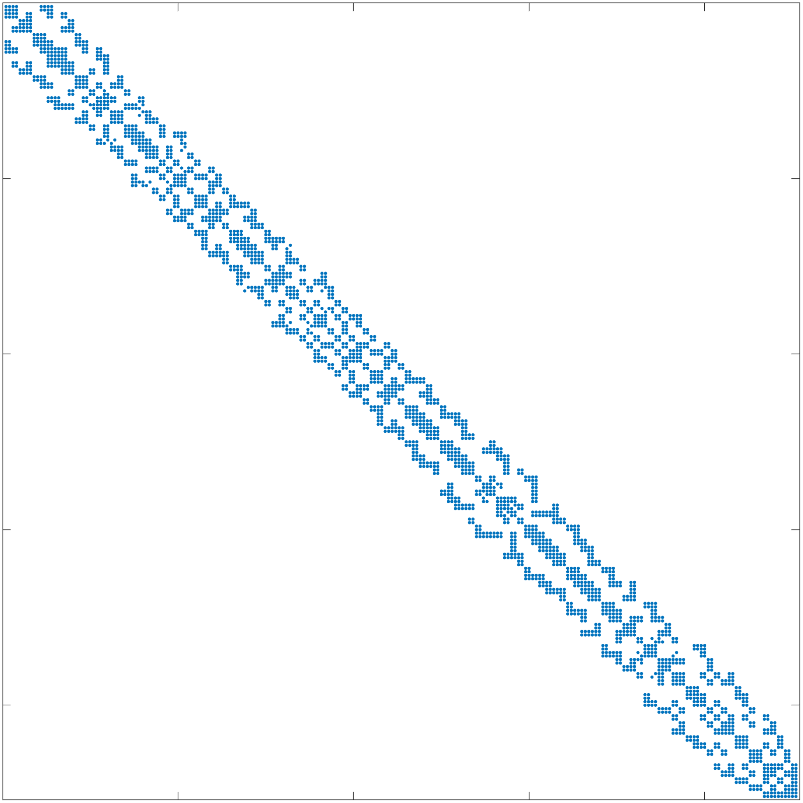
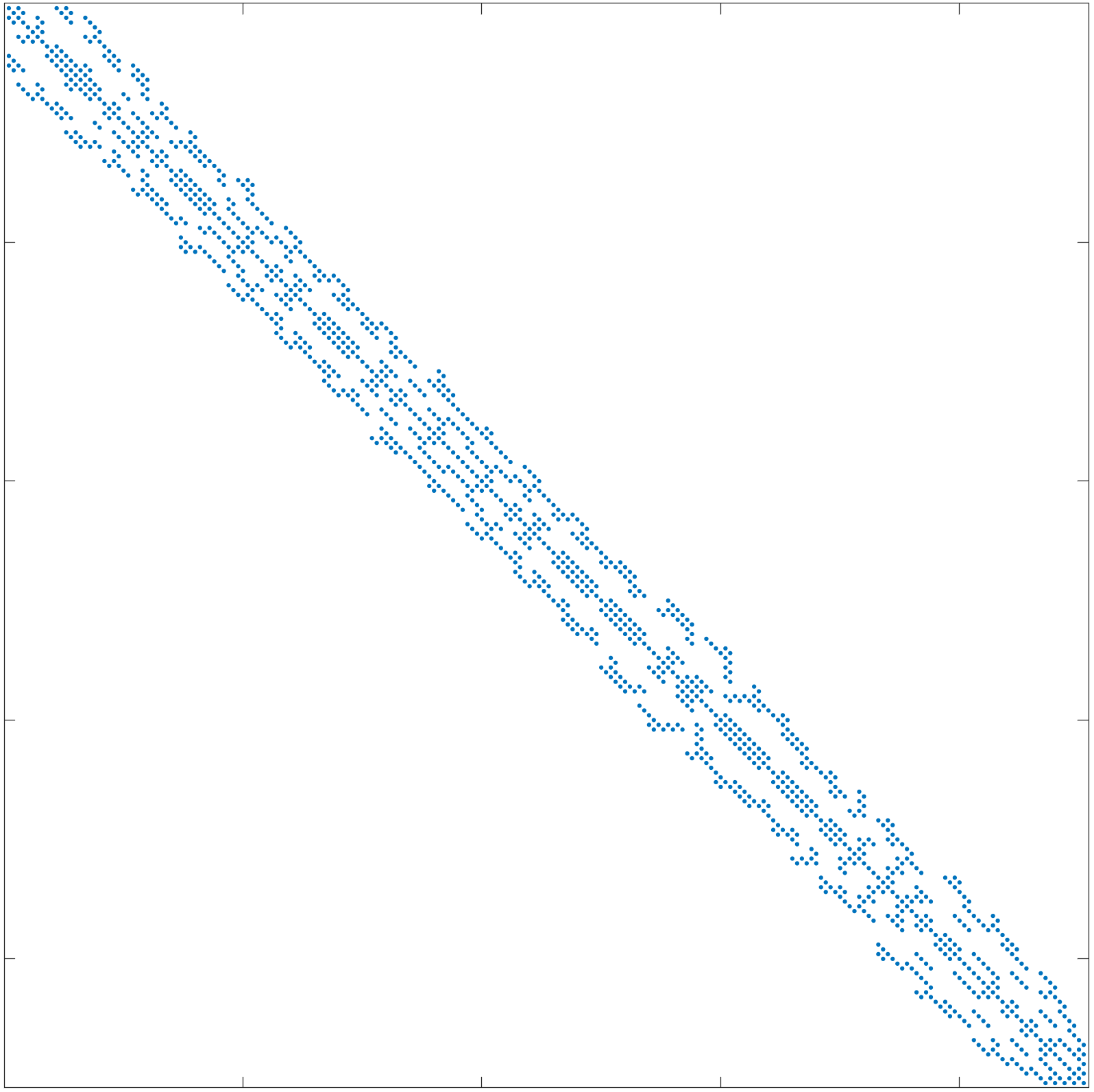
Figure 1: The structure of matrix pair $A$ (left) and $B$ (right) for $N=187778$.

5.2 Numerical Results

The numerical experiments are carried out by using PETSc [2] and SLEPc [18] in which MPI based distributed vectors and sparse matrices are provided. Besides CD and CRS method, numerical experiments for other compared methods are carried out by calling SLEPc. We set -eps_ncv 120 when $NEV=20$, and -eps_ncv 200 when $NEV=100$ for KrylovSchur method because this method performs worst or even fail with default setting, here -eps_ncv denotes the largest dimension of worrking subspace in KrylovShur method. The default parameters which are provided by SLEPc are used for all other cases.

The CRM (Conjugate Residual Method) without preconditioner is used as the linear solver, and zero vector is used as the initial vector for solving the RQI equation (11) in CRS method. We use the mark “-” to indicate that the computing time is more than two hours.

Numerical experiments were carried out on a cluster, all blade nodes are equipped with two 2.60GHz Intel(R) Xeon(R) Gold 6132 CPU, each CPU has 14 cores, and each node has 28 cores with 12 $\times$ 8GB DDR4 2400MHz ECC total 96GB memory.

Table 1: Numerical results for S1.

N	METHOD	NEV=20			NEV=100
		IT	MV	TIME(s)	IT	MV	TIME(s)
46958	KrylovSchur	153	26980	371.94	162	41565	857.92
	LOBPCG	125	14837	85.05	526	55806	336.00
	GD	4309	12375	83.76	15166	45103	996.25
	JD	136	40736	109.06	617	187075	609.32
	CD	1593	54272	114.76	6815	232242	543.66
	CRS	408	22167	63.74	1851	146996	309.86

In Table 1, we report the numerical results of scale S1 for computing $NEV$ smallest eigenvalues and the corresponding eigenvectors for the symmetric generalized eigenvalue problem (1) by using 1 processor. The restart number and the polynomial order involved in the CD and CRS method are set to be 80 and 30, respectively. And the number of iteration for solving RQI linear equation in CRS is set to 50.

From Table 1, we observe that KrylovSchur method takes the most time when $NEV=20$ and LOBPCG is more effective than JD. The CRS method is nearly twice faster than CD in term of computing time, and four times faster in term of number of iterations, respectively. JD and LOBPCG are slower than GD when $NEV=20$, but much faster when $NEV=100$. This shows that the block algorithm has great advantages for computing multiple eigenpairs. And we observe that among the seven methods the CRS method performs the best for both cases of $NEV=20$ and $NEV=100$, even though CRS is not a block algorithm.

Table 2: Numerical results for S2.

N	METHOD	NEV=20			NEV=100
		IT	MV	TIME(s)	IT	MV	TIME(s)
187778	KrylovSchur	379	66556	1630.36	357	89844	2258.28
	LOBPCG	332	38125	58.92	1421	138448	223.09
	GD	9812	28170	54.49	35450	105523	653.66
	JD	152	46176	36.46	697	215653	196.98
	CD	2501	110598	59.46	10558	466763	269.67
	CRS	456	40804	27.03	2026	251690	125.90

In Table 2, we report the numerical results of scale S2 for computing $NEV$ smallest eigenvalues and the corresponding eigenvectors for the symmetric generalized eigenvalue problem (1) by using 18 processors. The restart number and the polynomial order involved in the CD and CRS method are also set to be 80 and 40, respectively. The number of iteration for solving RQI linear equation in CRS is set to 90.

From Table 2, one can see that in both $NEV=20$ and $NEV=100$ cases, CRS performs the best by comparing the solution time. KrylovSchur is much slower than the other five methods. For this scale problem, JD method is more efficient than LOBPCG method. The number of iterations and computing time of CD are about 5 times and 2.2 times of CRS respectively.

Table 3: Numerical results for S3.

N	METHOD	NEV=20			NEV=100
		IT	MV	TIME(s)	IT	MV	TIME(s)
1143146	KrylovSchur	-	-	-	-	-	-
	LOBPCG	1062	128744	258.37	4820	465745	1026.06
	GD	25275	72567	195.19	93338	277951	2148.82
	JD	212	67219	79.27	794	250761	336.71
	CD	6326	281991	202.01	27676	1326207	893.43
	CRS	500	116908	83.57	2062	545207	332.87

In Table 3, we report the numerical results of scale S3 for computing $NEV$ smallest eigenvalues and the corresponding eigenvectors for the symmetric generalized eigenvalue problem (1) by using 112 processors. The restart number and the polynomial order involved in the CD and CRS method are also set to be 80 and 40, respectively. And the number of iteration for solving RQI linear equation in CRS is set to 250. We should remark that, in order to minimize the impact of communication between nodes, all experiments are done on the same 4 nodes.

From Table 3, we observe that KrylovSchur method fail. In this case, JD method is much more efficient, and it is about 3 times faster than LOBPCG method in term of computing time. The computing time of CD method are about 2 times more than that of CRS. JD and CRS methods perform best in this case. By comparing the results of CD and CRS from Tables 1–3, we can find that CRS performs better and better than CD with the increase of problem size.

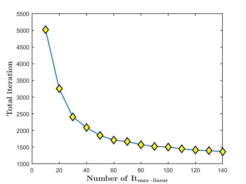
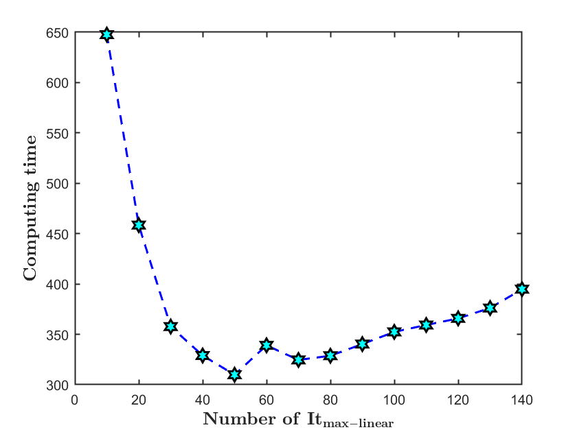
Figure 2: The total iteration (left) and computing time (right) of CRS method with different $\rm It_{\text{max-linear}}$ for S1 ($N=46958$, 1 processor).

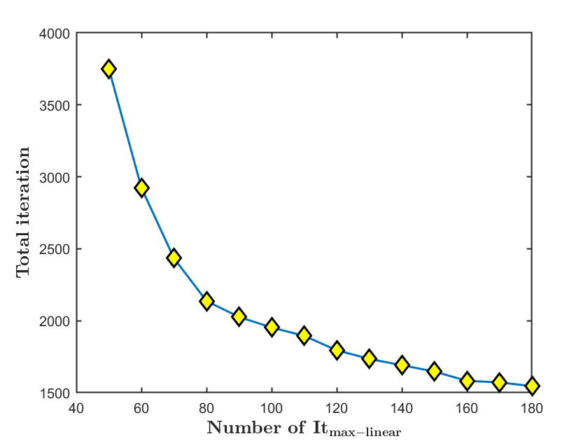
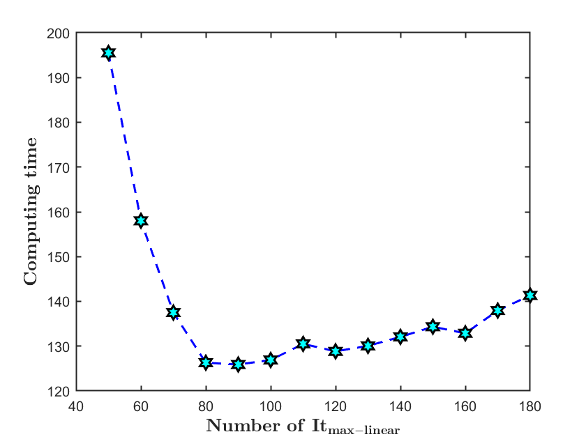
Figure 3: The total iteration (left) and computing time (right) of CRS method with different $\rm It_{\text{max-linear}}$ for S2 ($N=187778$, 18 processors).

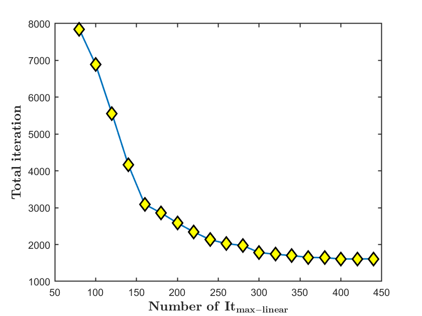
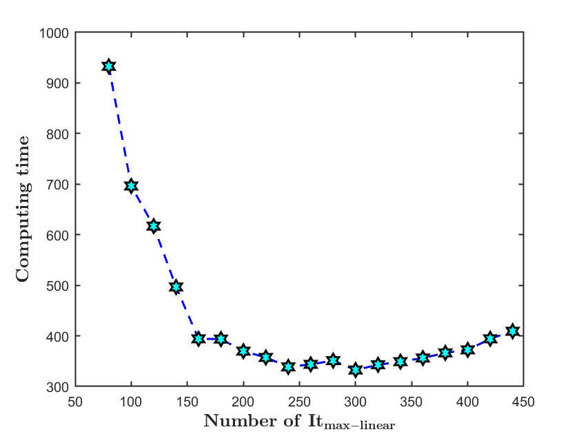
Figure 4: The total iteration (left) and computing time (right) of CRS method with different $\rm It_{\text{max-linear}}$ for S3 ($N=1143146$, 112 processors).

The number of linear iteration for solving the RQI equation is the most important ingredient affecting the performance of CRS method. In Figures 2, 3, and 4, the iteration numbers and computing time for solving these three scale problems are plotted with the increase of $\rm It_{\text{max-linear}}$, the maximal iteration number for solving the RQI linear equation. From these figures, we can find that, when $NEV=100$, the optimal value of $\rm It_{\text{max-linear}}$ is about 50 for S1 scale, 90 for S2 scale, and 250 for S3 scale in terms of computing time (where the polynomial order $m=30$ for S1, and $m=40$ for S2 and S3). The data in Tables 1–3 are obtained by using these optimal values. From these figures, one can also find that when the iteration number $\rm It_{\text{max-linear}}$ is greater than the optimal value, the CRS iteration decreases very little and the computing time increases not too much.

In the following, we show the strong scalability of several methods mentioned above for computing the first 20 smallest eigenpairs for two scales: $N=187778$ and $N=1143146$. For these two scale cases, the linear iteration number for solving the RQI equations is set to 90, and 250, respectively. The speedup curves for the strong scalability are plotted in Fig. 5. From this figure we observe that, among the four methods CRS has the best strong scalability. The line of CRS is almost linear when $N=187778$ (left) and superlinear when $N=1143146$ (right). We analyzed the time of each module in the algorithm and found that the time cost of ChebyshevFilter and CRM iteration decrease superlinearly.

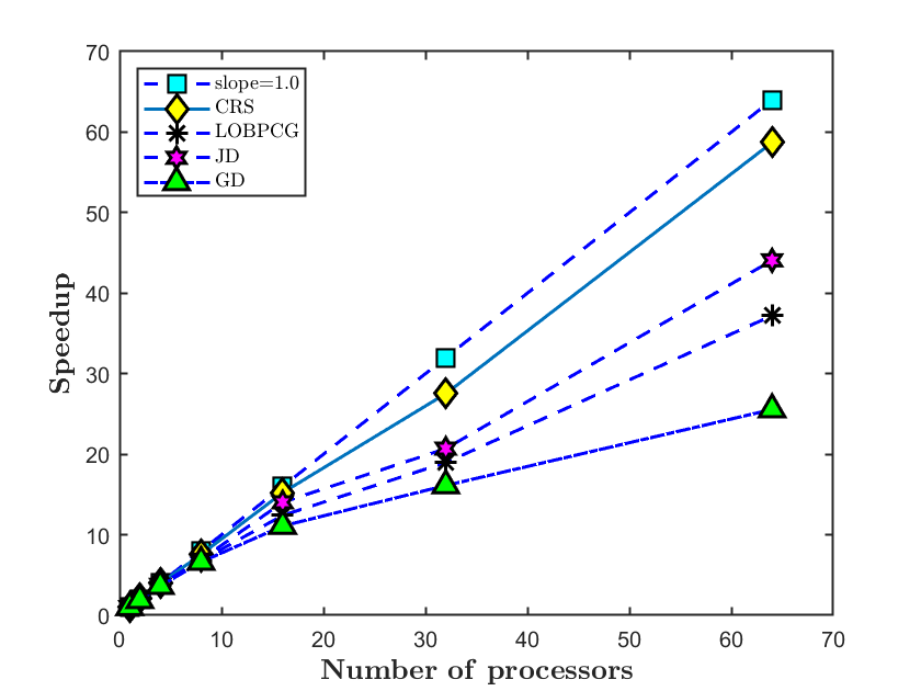
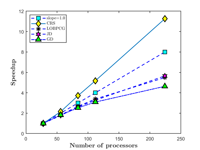
Figure 5: Strong scalability for four methods (left: $N=187778$; right: $N=1143146$).

At last in this section, it is necessary to point out that the number of restart is not a sensitive parameter in CRS. In numerical experiments, the algorithm converges within 40 iteration steps for computing one of the eigenpairs, i.e., the dimension of projection subspace would not exceed 80 and there is no need to restart. The restart parameter is set to prevent excessive storage for computing the eigenpairs which converge very slowly.

6 Concluding Remarks

In this paper, a new subspace algorithm for solving symmetric generalized eigenvalue problems is obtained by combining the technique of Chebyshev polynomial filter and inexact Rayleigh quotient iteration in the iteration process. The obtained method is named as CRS algorithm that can be used to compute several smallest eigenvalues and the corresponding eigenvectors.

Numerical results for a kind of vibration model show that the performance of the proposed algorithm is very good. Compared with some eigenvalue algorithms implemented in SLEPc, CRS method can compute multiple eigenpairs faster, and also it shows the best parallel scalability in our experiments. Therefore, CRS method has the potential to solve large scale eigenvalue problem in modal analysis of mechanical vibration.

In CRS method, it is needed to solve a linear equation related to RQI in each CRS iteration, and this is the dominant cost of CRS algorithm. For solving the linear equations, a Krylov subspace method (CRM) is employed. We studied the influence of the iteration number of Krylov method on the performance of the whole CRS algorithm. Numerical results show that a relatively optimal maximal iteration number is related to the scale of the problem.

For CRS algorithm, the following issues should be studied further:

• The method CRS proposed in this paper is a kind of one vector algorithm, that is, only one eigenpair can be obtained in each iteration. To compute multiple eigenpairs, block type method is usually preferable. It is deserved to consider the generalization of CRS to block version and the corresponding efficient implementation techniques for computing several eigenvalues simultaneously.

• In CRS method, one dominant cost is to solve the linear equation of RQI process. To trade off the convergence and efficiency, the problem is how to design a strategy to adjust the number of Krylov iteration adaptively for solving the linear equation. By increasing the number of Krylov iterations may make the convergence quickly, but at the same time, this will result in high computational costs and more computing time. This deserves to be studied furthermore to make the algorithm more effective.

• In this paper, only one iteration step of RQI is implemented in CRS algorithm to construct the augmented vector. One could also get an augmented vector by using several iteration steps of RQI iterations. This may result in a better augmented vector and CRS method may converge faster. As one linear equation should be solved in each iteration step of RQI, so if we use many iteration steps of RQI to produce the augmented vector, the cost will be much more expensive. Considering the whole efficiency of CRS method, this need to be studied further to trade off the iteration steps of RQI and the convergence rate of CRS algorithm.

Conflict of interest

The authors declare that they have no conflict of interest.

References

- [1] Arnoldi, W.E.: The principle of minimized iterations in the solution of the matrix eigenvalue problem. Quarterly of Applied Mathematics 9(1), 17–29 (1951)
- [2] Balay, S., Abhyankar, S., Adams, M., Brown, J., Brune, P., Buschelman, K., Dalcin, L., Dener, A., Eijkhout, V., Gropp, W., et al.: PETSc users manual (2019)
- [3] Bradbury, W., Fletcher, R.: New iterative methods for solution of the eigenproblem. Numerische Mathematik 9(3), 259–267 (1966)
- [4] Davidson, E.: The iterative calculation of a few of the lowest eigenvalues and corresponding eigenvectors of large real-symmetric matrices. Journal of Computational Physics 17, 87–94 (1975)
- [5] Fokkema, D.R., Sleijpen, G.L., Van der Vorst, H.A.: Jacobi–Davidson style QR and QZ algorithms for the reduction of matrix pencils. SIAM Journal on Scientific Computing 20(1), 94–125 (1998)
- [6] Golub, G.H., Van der Vorst, H.A.: Eigenvalue computation in the 20th century. Journal of Computational and Applied Mathematics 123(1-2), 35–65 (2000)
- [7] Hecht, F.: New development in FreeFem++. Journal of Numerical Mathematics 20(3-4), 251–266 (2012)
- [8] Hestenes, M.R., Karush, W.: A method of gradients for the calculation of the characteristic roots and vectors of a real symmetric matrix. Journal of Research of the National Bureau of Standards 47(1), 45–61 (1951)
- [9] Hochstenbach, M.E., Sleijpen, G.L.: Two-sided and alternating Jacobi–Davidson. Linear Algebra and its Applications 358(1-3), 145–172 (2003)
- [10] Jia, Z.: On convergence of the inexact Rayleigh quotient iteration with MINRES. Journal of Computational and Applied Mathematics 236(17), 4276–4295 (2012)
- [11] Knyazev, A.V.: Toward the optimal preconditioned eigensolver: locally optimal block preconditioned conjugate gradient method. SIAM Journal on Scientific Computing 23(2), 517–541 (2001)
- [12] Lanczos, C.: An iteration method for the solution of the eigenvalue problem of linear differential and integral operators (1950)
- [13] Lehoucq, R.B., Meerbergen, K.: Using generalized Cayley transformations within an inexact rational Krylov sequence method. SIAM Journal on Matrix Analysis and Applications 20(1), 131–148 (1998)
- [14] Li, Y., Wang, Z., Xie, H.: GCGE: A package for solving large scale eigenvalue problems by parallel block damping inverse power method. arXiv preprint arXiv:2111.06552 (2021)
- [15] Miao, C.Q.: On Chebyshev–Davidson method for symmetric generalized eigenvalue problems. Journal of Scientific Computing 85(3), 1–22 (2020)
- [16] Morgan, R.B., Scott, D.S.: Generalizations of Davidson’s method for computing eigenvalues of sparse symmetric matrices. SIAM Journal on Scientific and Statistical Computing 7(3), 817–825 (1986)
- [17] Parlett, B.N.: The Symmetric Eigenvalue Problem. SIAM (1998)
- [18] Roman, J.E., Campos, C., Romero, E., Tomás, A.: SLEPc users manual. D. Sistemes Informàtics i Computació Universitat Politècnica de València, Valencia, Spain, Report No. DSIC-II/24/02 (2015)
- [19] Ruhe, A.: Rational Krylov sequence methods for eigenvalue computation. Linear Algebra and its Applications 58, 391–405 (1984)
- [20] Saad, Y.: Numerical Methods for Large Eigenvalue Problems: revised edition. SIAM (2011)
- [21] Simoncini, V., Eldén, L.: Inexact Rayleigh quotient-type methods for eigenvalue computations. BIT Numerical Mathematics 42(1), 159–182 (2002)
- [22] Sleijpen, G.L., Booten, A.G., Fokkema, D.R., Van der Vorst, H.A.: Jacobi-Davidson type methods for generalized eigenproblems and polynomial eigenproblems. BIT Numerical Mathematics 36(3), 595–633 (1996)
- [23] Sleijpen, G.L., Van der Vorst, H.A.: A Jacobi–Davidson iteration method for linear eigenvalue problems. SIAM Review 42(2), 267–293 (2000)
- [24] Sorensen, D.C.: Implicit application of polynomial filters in a k-step Arnoldi method. SIAM Journal on Matrix Analysis and Applications 13(1), 357–385 (1992)
- [25] Sorensen, D.C.: Numerical methods for large eigenvalue problems. Acta Numerica 11, 519–584 (2002)
- [26] Stewart, G.W.: A Krylov–Schur algorithm for large eigenproblems. SIAM Journal on Matrix Analysis and Applications 23(3), 601–614 (2002)
- [27] Szyld, D.B., Xue, F.: Efficient preconditioned inner solves for inexact Rayleigh quotient iteration and their connections to the single-vector Jacobi–Davidson method. SIAM Journal on Matrix Analysis and Applications 32(3), 993–1018 (2011)
- [28] Vecharynski, E., Yang, C., Pask, J.E.: A projected preconditioned conjugate gradient algorithm for computing many extreme eigenpairs of a Hermitian matrix. Journal of Computational Physics 290, 73–89 (2015)
- [29] van der Vorst, H.A.: Computational methods for large eigenvalue problems (2002)
- [30] Zhou, Y.: Studies on Jacobi–Davidson, Rayleigh quotient iteration, inverse iteration generalized Davidson and Newton updates. Numerical Linear Algebra with Applications 13(8), 621–642 (2006)
- [31] Zhou, Y., Saad, Y.: A Chebyshev–Davidson algorithm for large symmetric eigenproblems. SIAM Journal on Matrix Analysis and Applications 29(3), 954–971 (2007)