The Voronoigram: Minimax Estimation of Bounded Variation Functions From Scattered Data

Abstract

We consider the problem of estimating a multivariate function $f_{0}$ of bounded variation (BV), from noisy observations $y_{i}=f_{0}(x_{i})+z_{i}$ made at random design points $x_{i}\in\mathbb{R}^{d}$, $i=1,\ldots,n$. We study an estimator that forms the Voronoi diagram of the design points, and then solves an optimization problem that regularizes according to a certain discrete notion of total variation (TV): the sum of weighted absolute differences of parameters $\theta_{i},\theta_{j}$ (which estimate the function values $f_{0}(x_{i}),f_{0}(x_{j})$) at all neighboring cells $i,j$ in the Voronoi diagram. This is seen to be equivalent to a variational optimization problem that regularizes according to the usual continuum (measure-theoretic) notion of TV, once we restrict the domain to functions that are piecewise constant over the Voronoi diagram.

The regression estimator under consideration hence performs (shrunken) local averaging over adaptively formed unions of Voronoi cells, and we refer to it as the Voronoigram, following the ideas in Koenker (2005), and drawing inspiration from Tukey’s regressogram (Tukey, 1961). Our contributions in this paper span both the conceptual and theoretical frontiers: we discuss some of the unique properties of the Voronoigram in comparison to TV-regularized estimators that use other graph-based discretizations; we derive the asymptotic limit of the Voronoi TV functional; and we prove that the Voronoigram is minimax rate optimal (up to log factors) for estimating BV functions that are essentially bounded.

1 Introduction

Consider a standard nonparametric regression setting, given observations $(x_{i},y_{i})\in\Omega\times\mathbb{R}$, $i=1,\dots,n$, for an open and connected subset $\Omega$ of $\mathbb{R}^{d}$, and with

$$y_{i}=f_{0}(x_{i})+z_{i},\quad i=1,\dots,n,$$ (1)

for i.i.d. mean zero stochastic errors $z_{i}$, $i=1,\dots,n$. We are interested in estimating the function $f_{0}$ under the working assumption that $f_{0}$ adheres to a certain notion of smoothness. A traditional smoothness assumption on $f_{0}$ involves its integrated squared derivatives, for example, the assumption that

$$\int_{\Omega}\sum_{\|\alpha\|_{1}=2}(D^{\alpha}f)^{2}(x)\,dx$$

is small, where $\alpha=(\alpha_{1},\dots,\alpha_{d})\in\mathbb{Z}_{+}^{d}$ is a multi-index and we write $D^{\alpha}=\frac{\partial^{\alpha_{1}}}{\partial x_{1}}\dots\frac{\partial^{\alpha_{d}}}{\partial x_{d}}$ for the corresponding mixed partial derivative operator. This is the notion of smoothness that underlies the celebrated smoothing spline estimator in the univariate case $d=1$ (Schoenberg, 1964) and the thin-plate spline estimator when $d=2$ or 3 (Duchon, 1977). We also note that assuming $f_{0}$ is smooth in the sense of the above display is known as second-order $L^{2}$ Sobolev smoothness (where we interpret $D^{\alpha}f$ as a weak derivative).

Smoothing splines and thin-plate splines are quite popular and come with a number of advantages. However, one shortcoming of using these methods, i.e., to using the working model of Sobolev smoothness, is that it does not permit $f_{0}$ to have discontinuities, which limits its applicability. More broadly, smoothing splines and thin-plate splines do not fare well when the estimand $f_{0}$ possesses heterogeneous smoothness, meaning that $f_{0}$ is more smooth at some parts of its domain $\Omega$ and more wiggly at others. This motivates us to consider regularity measured by the total variation (TV) seminorm

$$\operatorname{\mathrm{TV}}(f;\Omega)=\sup\left\{\int_{\Omega}f(x)\operatorname{\mathrm{div}}\phi(x)\,dx:\phi\in C_{c}^{1}(\Omega;\mathbb{R}^{d}),\,\|\phi(x)\|_{2}\leq 1\;\text{for all $x\in\Omega$}\right\},$$ (2)

where $C_{c}^{1}(\Omega;\mathbb{R}^{d})$ denotes the space of continuously differentiable compactly supported functions from $\Omega$ to $\mathbb{R}^{d}$, and we use $\operatorname{\mathrm{div}}\phi=\sum_{i=1}^{d}\partial\phi_{i}/\partial_{x_{i}}$ for the divergence of $\phi=(\phi_{1},\dots,\phi_{d})$. Accordingly, we define the bounded variation (BV) class on $\Omega$ by

$$\operatorname{\mathrm{BV}}(\Omega)=\{f\in L^{1}(\Omega):\operatorname{\mathrm{TV}}(f;\Omega)<\infty\},$$

to contain all $L^{1}(\Omega)$ functions with finite TV. The definition in (2) is often called the measure-theoretic definition of multivariate TV. For simplicity we will often drop the notational dependence on $\Omega$ and simply write this as $\operatorname{\mathrm{TV}}(f)$. This definition may appear complicated at first, but it admits a few natural interpretations, which we present next to help build intuition.

1.1 Perspectives on total variation

Below are three perspectives on total variation. The first two reveal the way that TV acts on special types of functions; the third is a general equivalent form of TV.

Smooth functions.

If $f$ is (weakly) differentiable with (weak) gradient $\nabla f=(\frac{\partial f}{\partial x_{1}},\dots,\frac{\partial f}{\partial x_{d}})$, then

$$\operatorname{\mathrm{TV}}(f)=\int_{\Omega}\|\nabla f(x)\|_{2}\,dx,$$ (3)

provided that the right-hand here is well-defined and finite. Consider the difference between this and the first-order $L^{2}$ Sobolev seminorm

$$\int_{\Omega}\sum_{\|\alpha\|_{1}=1}(D^{\alpha}f)^{2}(x)\,dx=\int_{\Omega}\|\nabla f(x)\|_{2}^{2}\,dx.$$

The latter uses the squared $\ell_{2}$ norm $\|\cdot\|_{2}^{2}$ in the integrand, whereas the former (3) uses the $\ell_{2}$ norm $\|\cdot\|_{2}$. It turns out that this is a meaningful difference—one way to interpret this is as a difference between $L^{2}$ and $L^{1}$ regularity. Noting that $\|x\|_{1}\leq\sqrt{d}\|x\|_{2}$ for all $x\in\mathbb{R}^{d}$, the space $\operatorname{\mathrm{BV}}(\Omega)$ contains the first-order $L^{1}$ Sobolev space

$$W^{1,1}(\Omega)=\{f\in L^{1}(\Omega):\int_{\Omega}\|\nabla f(x)\|_{1}\,dx<\infty\},$$

which, loosely speaking, contains functions that can be more locally peaked and less evenly spread out (i.e., permits a greater degree of heterogeneity in smoothness) compared to the first-order $L^{2}$ Sobolev space

$$W^{1,2}(\Omega)=\{f\in L^{2}(\Omega):\int_{\Omega}\|\nabla f(x)\|_{2}^{2}\,dx<\infty\}.$$

It is important to emphasize, however, that $\operatorname{\mathrm{BV}}(\Omega)$ is still much larger than $W^{1,1}(\Omega)$, because it permits functions to have sharp discontinuities. We discuss this next.

Indicator functions.

If $S\subseteq\Omega$ is a set with locally finite perimeter, then the indicator function $1_{S}$, which we define by $1_{S}(x)=1$ for $x\in S$ and $0$ otherwise, satisfies

$$\operatorname{\mathrm{TV}}(1_{S})=\mathrm{per}(S),$$ (4)

where $\mathrm{per}(S)$ is the perimeter of $S$ (or equivalently, the codimension 1 Hausdorff measure of $\partial S$, the boundary of $S$). Thus, we see that that TV is tied to the geometry of the level sets of the function in question. Indeed, there is a precise sense in which this is true in full generality, as we discuss next.

Coarea formula.

In general, for any $f\in\operatorname{\mathrm{BV}}(\Omega)$, we have

$$\operatorname{\mathrm{TV}}(f)=\int_{-\infty}^{\infty}\mathrm{per}\big{(}\{x\in\Omega:f(x)>t\}\big{)}\,dt.$$ (5)

This is known as the coarea formula for BV functions (see, e.g., Theorem 5.9 in Evans and Gariepy, 2015). It offers a highly intuitive picture of what total variation is measuring: we take a slice through the graph of a function $f$, calculate the perimeter of the set of points (projected down to the $\Omega$-axis) that lie above this slice, and add up these perimeters over all possible slices.

The coarea formula (5) also sheds light on why BV functions are able to portray such a great deal of heterogeneous smoothness: all that matters is the total integrated amount of function growth, according to the perimeter of the level sets, as we traverse the heights of level sets. For example, if the perimeter has a component $\rho$ that persists for a range of level set heights $[t,t+h]$, then this contributes the same amount $\rho h$ to the TV as does a smaller perimeter component $\rho/100$ that persists for a larger range of level set heights $[t,t+100h]$. To put it differently, the former might represent a local behavior that is more spread out, and the latter a local behavior that is more peaked, but these two behaviors can contribute the same amount to the TV in the end. Therefore, a ball in the BV space—all $L^{1}$ functions $f$ such that $\operatorname{\mathrm{TV}}(f)\leq r$—contains functions with a huge variety in local smoothness.

1.2 Why is estimating BV functions hard?

Now that we have motivated the study of BV functions, let us turn towards the problem of estimating a BV function from noisy samples. Given the centrality of penalized empirical risk minimization in nonparametric regression, one might be tempted to solve the TV-penalized variational problem

$$\mathop{\mathrm{minimize}}_{f\in\operatorname{\mathrm{BV}}(\Omega)}\;\frac{1}{2}\sum_{i=1}^{n}(y_{i}-f(x_{i}))^{2}+\lambda\operatorname{\mathrm{TV}}(f),$$ (6)

given data $(x_{i},y_{i})$, $i=1,\dots,n$ from the model (1), and under the working assumption that $f$ has small TV. However, in short, solving (6) will “not work” in any dimension $d\geq 2$, in the sense that it does not yield a well-defined estimator regardless of the choice of tuning parameter $\lambda>0$.

When $d=1$, solving (6) produces a celebrated estimator known as the (univariate) TV denoising estimator (Rudin et al., 1992) or the fused lasso signal approximator (Tibshirani et al., 2005). (More will be said about this shortly, under the related work subsection.) But for any $d\geq 2$, problem (6) is ill-posed, as the criterion does not achieve its infimum. To see this, consider the function

$$f_{\epsilon}=\sum_{i=1}^{n}y_{i}\cdot 1_{B(x_{i},\epsilon)},$$

where $B(x_{i},\epsilon)$ denotes the closed $\ell_{2}$ ball of radius $\epsilon$ centered at $x_{i}$, and $1_{B(x_{i},\epsilon)}$ denotes its indicator function (which equals 1 on $B(x_{i},\epsilon)$ and 0 outside of it). Now let us examine the criterion in problem (6): for small enough $\epsilon>0$, the function $f_{\epsilon}$ has a squared loss equal to 0, and has TV penalty equal to $\lambda nc_{d}\epsilon^{d-1}$ (here $c_{d}>0$ is a constant depending only on $d$). Hence, as $\epsilon\to 0$, the criterion value in (6) achieved by $f_{\epsilon}$ tends to 0. However, as $\epsilon\to 0$, the function $f_{\epsilon}$ itself trivially approaches the zero function, defined as $f(x)=0$ for all $x$. Note that this is true for any $\lambda>0$, whereas the zero function certainly cannot minimize the objective in (6) for all $\lambda>0$.

The problem here, informally speaking, is that the BV class is “too big” when $d\geq 2$; more formally, the evaluation operator is not continuous over the BV space—or in other words, convergence in BV norm does not imply pointwise convergence—for $d\geq 2$. It is worth noting that this problem is not specific to BV spaces and it also occurs with the $k^{\text{th}}$ order $L^{p}$ Sobolev space $W^{k,p}(\Omega)=\{f\in L^{p}:\int_{\Omega}\sum_{\|\alpha\|_{1}=k}(D^{\alpha}f)^{p}(x)\,dx<\infty\}$ when $pk\leq d$, which is called the subcritical regime. In the supercritical regime $pk>d$, convergence in Sobolev norm implies pointwise convergence, but all bets are off when $pk\leq d$. Thus, just as the TV-penalized problem (6) is ill-posed for $d\geq 2$, the more familiar thin-plate spline problem

$$\mathop{\mathrm{minimize}}_{f\in W^{2,2}(\Omega)}\;\frac{1}{2}\sum_{i=1}^{n}(y_{i}-f(x_{i}))^{2}+\lambda\int_{\Omega}\|\nabla^{2}f(x)\|_{F}^{2}\,dx$$

is itself ill-posed when $d\geq 4$. (Here we use $\nabla^{2}f(x)$ for the weak Hessian of $f$, and $\|\cdot\|_{F}$ for the Frobenius norm, so that the second-order $L^{2}$ Sobolev seminorm can be written as $\int_{\Omega}\sum_{\|\alpha\|_{1}=2}(D^{\alpha}f)^{2}(x)\,dx=\int_{\Omega}\|\nabla^{2}f(x)\|_{F}^{2}\,dx$.)

What can we do to circumvent this issue? Broadly speaking, previous approaches from the literature can be stratified into two types. The first maintains the smoothness assumption on $\operatorname{\mathrm{TV}}(f_{0})$ for the regression function $f_{0}$, but replaces the sampling model (1) by a white noise model of the form

$$dY(x)=f_{0}(x)dx+\frac{\sigma}{\sqrt{n}}dW(x),\quad x\in\Omega,$$

where $dW$ is a Gaussian white noise process. Given this continuous-space observation model, we can then replace the empirical loss term $\sum_{i=1}^{n}(y_{i}-f(x_{i}))^{2}$ in (6) by the squared $L^{2}$ loss $\|Y-f\|_{L^{2}(\Omega)}^{2}=\int_{\Omega}(Y(x)-f(x))^{2}\,dx$ (or some multiscale variant of this). The second type of approach keeps the sampling model (1), but replaces the assumption on $\operatorname{\mathrm{TV}}(f_{0})$ by an assumption on discrete total variation (which is based on the evaluations of $f_{0}$ at the design points alone) of the form

$$\operatorname{\mathrm{DTV}}(f_{0})=\sum_{\{i,j\}\in E}w_{ij}|f_{0}(x_{i})-f_{0}(x_{j})|,$$

for an edge set $E$ and weights $w_{ij}\geq 0$. We then naturally replace the penalty $\operatorname{\mathrm{TV}}(f)$ in (6) by $\operatorname{\mathrm{DTV}}(f)$. More details on both types of approaches will be given in the related work subsection.

The approach we take in the current paper sits in the middle, between the two types. Like the first, we maintain a bona fide smoothness assumption on $\operatorname{\mathrm{TV}}(f_{0})$, rather than a discrete version of TV. Like the second, we work in the sampling model (1), and define an estimator by solving a discrete version of (6) which is always well posed, for any dimension $d\geq 2$. In fact, the connections run deeper: the discrete problem that we solve is not constructed arbitrarily, but comes from restricting the domain in (6) to a special finite-dimensional class of functions, over which the penalty $\operatorname{\mathrm{TV}}(f)$ in (6) takes on an equivalent discrete form.

1.3 The Voronoigram

This brings us to the central object in the current paper: an estimator defined by restricting the domain in the infinite-dimensional problem (6) to a finite-dimensional subspace, whose structure is governed by the Voronoi diagram of the design points $x_{1},\dots,x_{n}\in\Omega$. In detail, let $V_{i}=\{x\in\Omega:\|x_{i}-x\|_{2}<\|x_{j}-x\|\}$ be the Voronoi cell associated with $x_{i}$, for $i=1,\dots,n$, and define

$$\mathcal{F}^{\mathrm{V}}_{n}=\mathrm{span}\big{\{}1_{V_{1}},\dots,1_{V_{n}}\big{\}},$$

where recall $1_{V_{i}}$ is the indicator function of $V_{i}$. In words, $\mathcal{F}^{\mathrm{V}}_{n}$ is a space of functions from $\Omega$ to $\mathbb{R}$ that are piecewise constant on the Voronoi diagram of $x_{1},\dots,x_{n}$. (We remark that this is most certainly a subspace of $\operatorname{\mathrm{BV}}(\Omega)$, as each Voronoi cell has locally finite perimeter; in fact, as we will see soon, the TV of each $f\in\mathcal{F}^{\mathrm{V}}_{n}$ takes a simple and explicit closed form.) Now consider the finite-dimensional problem

$$\mathop{\mathrm{minimize}}_{f\in\mathcal{F}^{\mathrm{V}}_{n}}\;\frac{1}{2}\sum_{i=1}^{n}(y_{i}-f(x_{i}))^{2}+\lambda\operatorname{\mathrm{TV}}(f).$$ (7)

We call the solution to (7) the Voronoigram and denote it by $\hat{f}^{\mathrm{V}}$. This idea—to fit a piecewise constant function to the Voronoi tessellation of the input domain $\Omega$—dates back to (at least) Koenker (2005), where it was briefly proposed in Chapter 7 of this book (further discussion of related work will be given in Section 1.5). It does not appear to have been implemented or studied beyond this. Its name is inspired by Tukey’s classic regressogram (Tukey, 1961).

Of course, there a many choices for a finite-dimensional subset of $\operatorname{\mathrm{BV}}(\Omega)$ that we could have used for a domain restriction in (7). Why $\mathcal{F}^{\mathrm{V}}_{n}$, defined by piecewise constant functions on the Voronoi diagram, as in (7)? A remarkable feature of this choice is that it yields an equivalent optimization problem

$$\mathop{\mathrm{minimize}}_{\theta\in\mathbb{R}^{n}}\;\frac{1}{2}\sum_{i=1}^{n}(y_{i}-\theta_{i})^{2}+\lambda\sum_{\{i,j\}\in E^{\mathrm{V}}}w^{\mathrm{V}}_{ij}\cdot|\theta_{i}-\theta_{j}|,$$ (8)

for an edge set $E^{\mathrm{V}}$ defined by neighbors in the Voronoi graph, and weights $w^{\mathrm{V}}_{ij}$ that measure the “length” of the shared boundary between cells $V_{i}$ and $V_{j}$, to be defined precisely later (in Section 2.1). The equivalence between problems (7) and (8) sets $\theta_{i}=f(x_{i})$, $i=1,\dots,n$, and is driven by the following special fact: for such a pairing, whenever $f\in\mathcal{F}^{\mathrm{V}}_{n}$, it holds (proved in Section 2.1) that

$$\operatorname{\mathrm{TV}}(f)=\sum_{\{i,j\}\in E^{\mathrm{V}}}w^{\mathrm{V}}_{ij}\cdot|\theta_{i}-\theta_{j}|.$$ (9)

In this way we can view the Voronoigram as marriage between a purely variational approach, which maintains the use of a continuum TV penalty on a function $f$, and a purely discrete approach, which instead models smoothness using a discrete TV penalty on a vector $\theta$ defined over a graph. In short, the Voronoigram does both.

1.3.1 A first look at the Voronoigram

From its equivalent discrete problem form (8), we can see that the penalty term drives the Voronoigram to have equal (or “fused”) evaluations at points $x_{i}$ and $x_{j}$ corresponding to neighboring cells in the Voronoi tessellation. Generally, the larger the value of $\lambda\geq 0$, the more neighboring evaluations will be fused together. Due to fact that each $f\in\mathcal{F}^{\mathrm{V}}_{n}$ is constant over an entire Voronoi cell, this means that the Voronoigram fitted function $\hat{f}^{\mathrm{V}}$ is constant over adaptively chosen unions of Voronoi cells. Furthermore, based on what is known about solutions of generalized lasso problems (details given in Section 2.2), we can express the fitted function here as

$$\hat{f}^{\mathrm{V}}=\sum_{k=1}^{\hat{K}}(\bar{y}_{k}-\hat{s}_{k})\cdot 1_{\hat{R}_{k}},$$ (10)

where $\hat{K}$ is the number of connected components that appear in the solution $\hat{\theta}^{\mathrm{V}}$ over the Voronoi graph, $\hat{R}_{k}$ denotes a union of Voronoi cells associated with the $k^{\text{th}}$ connected component, $\bar{y}_{k}$ denotes the average of response points $y_{i}$ such that $x_{i}\in\hat{R}_{k}$; and $\hat{s}_{k}$ is a data-driven shrinkage factor. To be clear, each of $\hat{K}$, $\hat{R}_{k}$, $\bar{y}_{k}$, and $\hat{s}_{k}$ here are data-dependent quantities—they fall out of the structure of the solution in problem (8).

Thus, like the regressogram, the Voronoigram estimates the regression function by fitting (shrunken) averages over local regions; but unlike the regressogram, where the regions are fixed ahead of time, the Voronoigram is able to choose its regions adaptively, based on the geometry of the design points $x_{i}$ (owing to the use of the Voronoi diagram) and on how much local variation is present in the response points $y_{i}$ (a consideration inherent to the minimization in (8), which trades off between the loss and penalty summands).

Figure 1 gives a simple example of the Voronoigram and its adaptive structure in action.

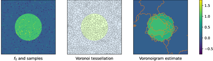
Figure 1: A simple example of using the Voronoigram to estimate a function $f_{0}$, from noisy observations. Left: $f_{0}$ and noisy observations made at $n=1274$ random points in $d=2$ dimensions. Center: the Voronoi tessellation, whose cells constitute the piecewise constant basis for the Voronoigram. Right: the Voronoigram estimate (at a certain choice of $\lambda$), with the resulting adaptively chosen constant pieces—over which it performs averaging—outlined in orange.

1.4 Summary of contributions

Our primary practical and methodological contribution is to motivate and study the Voronoigram as a nonparametric regression estimator for BV functions in a multivariate scattered data (random design) setting, including comparing and contrasting it to two related approaches: discrete TV regularization using $\varepsilon$-neighborhood or $k$-nearest neighbor graphs. A summary is as follows (a more detailed summary is given in Section 2.4).

• The graph used by Voronoigram—namely, the Voronoi adjacency graph—is tuning-free. This stands in contrast to $\varepsilon$-neighborhood or $k$-nearest neighbor graphs, which require a choice of a local radius $\varepsilon$ or number of neighbors $k$, respectively.

• The Voronoigram penalty becomes density-free in large samples, which is term we use to describe the fact that it converges to “pure” total variation, independent of the density $p$ of the (random) design points $x_{1},\dots,x_{n}$. This follows from one of our main theoretical results (reiterated below), and it stands in contrast to the TV penalties based on $\varepsilon$-neighborhood and $k$-nearest neighbor graphs, which are known to asymptotically approach particular $p$-weighted versions of total variation.

• The Voronoigram estimator yields a natural passage from a discrete set of fitted values $\hat{f}^{\mathrm{V}}(x_{i})$, $i=1,\dots,n$ to a fitted function $\hat{f}^{\mathrm{V}}$ defined over the entire input domain $\Omega$: this is simply given by local constant extrapolation of each fitted value $\hat{f}^{\mathrm{V}}(x_{i})$ to its containing Voronoi cell $V_{i}$. (Equivalently, $\hat{f}^{\mathrm{V}}(x)$ is given by the 1-nearest neighbor prediction rule based on $(x_{i},\hat{f}^{\mathrm{V}}(x_{i}))$, $i=1,\dots,n$.) Further, thanks to (9), we know that such an extrapolation method is complexity-preserving: the discrete TV of $\hat{\theta}^{\mathrm{V}}_{i}$, $i=1,\ldots,n$ is precisely the same as the continuum TV of the extrapolant $\hat{f}^{\mathrm{V}}$. Other graph-based TV regularization methods do not come with this property.

On the theoretical side, our primary theoretical contributions are twofold, summarized below.

• We prove that the Voronoi penalty functional, applied to evaluations of $f$ at i.i.d. design points $x_{1},\ldots,x_{n}$ from a density $p$, converges to $\operatorname{\mathrm{TV}}(f)$, as $n\to\infty$ (see Section 3 for details). The fact that its asymptotic limit here is independent of $p$ is both important and somewhat remarkable.

• We carry out a comprehensive minimax analysis for $L^{2}$ estimation over $\operatorname{\mathrm{BV}}(\Omega)$. The highlights (Section 5 gives details): for any fixed $d\geq 2$ and regression function $f_{0}$ with $\operatorname{\mathrm{TV}}(f_{0})\leq L$ and $\|f_{0}\|_{L^{\infty}}\leq M$ (where $L,M>0$ are constants), a modification of the Voronoigram estimator $\hat{f}^{\mathrm{V}}$ in (7)—defined by simply clipping small weights $w^{\mathrm{V}}_{ij}$ in the penalty term—converges to $f_{0}$ at the squared $L^{2}$ rate $n^{-1/d}$ (ignoring log terms). We prove that this matches the minimax rate (up to log terms) for estimating a regression function $f_{0}$ that is bounded in TV and $L^{\infty}$. Lastly, we prove that an even simpler unweighted Voronoigram estimator—defined by setting all edge weights in (7) to unity—also obtains the optimal rate (up to log terms), as do more standard estimators based on discrete TV regularization over $\varepsilon$-neighborhood and $k$-nearest neighbor graphs.

1.5 Related work

The work of Mammen and van de Geer (1997) marks an important early contribution promoting and studying the use of TV as a regularization functional, in univariate nonparametric regression. These authors considered a variational problem similar to (6) in dimension $d=1$, with a generalized penalty $\operatorname{\mathrm{TV}}(D^{k}f)$, the TV of the $k^{\text{th}}$ weak derivative $D^{k}f$ of $f$. They proved that the solution is always a spline of degree $k$ (whose knots may lie outside the design points if $k\geq 2$) and named the solution the locally adaptive regression spline estimator. A related, more recent idea is trend filtering, proposed by Steidl et al. (2006); Kim et al. (2009) and extended by Tibshirani (2014) to the case of arbitrary design points. Trend filtering solves a discrete analog of the locally adaptive regression spline problem, in which the penalty $\operatorname{\mathrm{TV}}(D^{k}f)$ is replaced by the discrete TV of the $k^{\text{th}}$ discrete derivative of $f$—based entirely on evaluations of $f$ at the design points.

Tibshirani (2014) showed that trend filtering, like the Voronoigram, admits a special duality between discrete and continuum representations: the trend filtering optimization problem is in fact the restriction of the variational problem for locally adaptive regression splines to a particular finite-dimensional space of $k^{\text{th}}$ degree piecewise polynomials. The key fact underlying this equivalence is that for any function $f$ in this special piecewise polynomial space, its continuum penalty $\operatorname{\mathrm{TV}}(D^{k}f)$ equals its discrete penalty (discrete TV applied to its $k^{\text{th}}$ discrete derivatives), a result analogous to the property (9) of functions $f\in\mathcal{F}^{\mathrm{V}}_{n}$. Thus we can view the Voronoigram a generalization of this core idea, at the heart of trend filtering, to multiple dimensions—albeit restricted the case $k=0$.

We note that similar ideas to locally adaptive regression splines and trend filtering were around much earlier; see, e.g., Schuette (1978); Koenker et al. (1994). Tibshirani (2022) provides an account of the history of these and related ideas in nonparametric smoothing, and also makes connections to numerical analysis—the study of discrete splines in particular. It is worth highlighting that when $k=0$, the locally adaptive regression spline and trend filtering estimators coincide, and reduce to a method known as TV denoising, which has even earlier roots in applied mathematics (to be covered shortly).

Beyond the univariate setting, there is still a lot of related work to cover across different areas of the literature, and we break up our exposition into parts accordingly.

Continuous-space TV methods.

The seminal work of Rudin et al. (1992) introduced TV regularization in the context of signal and image denoising, and has spawned to a large body of follow-up work, mostly in the applied mathematics community, where this is called the Rudin-Osher-Fatemi (ROF) model for TV denoising. See, e.g., Rudin and Osher (1994); Vogel and Oman (1996); Chambolle and Lions (1997); Chan et al. (2000), among many others. In this literature, the observation model is traditionally continuous-time (univariate), or continuous-space (multivariate)—this means that, rather than having observations at a finite set of design points, we have an entire observation process (deterministic or random), itself a function over a bounded and connected subset of $\mathbb{R}^{d}$. TV regularization is then used in a variational optimization context, and discretization usually occurs (if at all) as part of numerical optimization schemes for solving such variational problems.

Statistical analysis in continuous-space observation models traditionally assumes a white noise regression model, which has a history of study for adaptive kernel methods (via Lepski’s method) or wavelet methods in particular, see, e.g., Lepski et al. (1997); Lepski and Spokoiny (1997); Neumann (2000); Kerkyacharian et al. (2001, 2008). In this general area of the literature, the recent paper of del Álamo et al. (2021) is most related to our paper: these authors consider a multiresolution TV-regularized estimator in a multivariate white noise model, and derive minimax rates for $L^{p}$ estimation of TV and $L^{\infty}$ bounded functions. When $p=2$, they establish a minimax rate (ignoring log factors) of $n^{-1/d}$ on the squared $L^{2}$ error scale, for arbitrary dimension $d\geq 2$, which agrees with our results in Section 5.

Discrete, lattice-based TV methods.

Next we discuss purely discrete TV-regularization approaches, in which both the observation model and the penalty are discrete, and are based on function values at a discrete sequence of points. Such approaches can be further delineated into two subsets: models and methods based on discrete TV over lattices (multi-dimensional grid graphs), and those based on discrete TV over geometric graphs (such as $\varepsilon$-neighborhood or $k$-nearest neighbor graphs constructed from the design points). We cover the former first, and the latter second.

For lattice-based TV approaches, Tibshirani et al. (2005) marks an early influential paper studying discrete TV regularization over univariate and bivariate lattices, under the name fused lasso. This generated much follow-up work in statistics, e.g., Friedman et al. (2007); Hoefling (2010); Tibshirani and Taylor (2011); Arnold and Tibshirani (2016), among many others. In terms of theory, we highlight Hutter and Rigollet (2016), who established sharp upper bounds for the estimation error of TV denoising over lattices, as well as Sadhanala et al. (2016), who certified optimality (up to log factors) by giving minimax lower bounds. The rate here (ignoring log factors) for estimating signals with bounded discrete TV, in mean squared error across the lattice points, is $n^{-1/d}$. This holds for an arbitrary dimension $d\geq 2$, and agrees with our results in Section 5. Interestingly, Sadhanala et al. (2016) also prove that the minimax linear rate over the discrete TV is class is constant—which means that the best estimator that is linear in the response vector $y\in\mathbb{R}^{n}$, of the form $\hat{f}(x)=w(x)^{\mathsf{T}}y$, is inconsistent in terms of its max risk (over signals with bounded discrete TV). We do not pursue minimax linear analysis in the current paper but expect a similar phenomenon to hold in our setting.

Lastly, we highlight Sadhanala et al. (2017, 2021), who proposed and studied an extension of trend filtering on lattices. Just like univariate trend filtering, the multivariate version allows for an arbitrary smoothness order $k\geq 0$, and reduces to TV denoising (or the fused lasso) on a lattice for $k=0$. In the lattice setting, the theoretical picture is fairly complete: for general $k,d$, denoting by $s=(k+1)/d$ the effective degree of smoothness, the minimax rate for estimating signals with bounded $k^{\text{th}}$ order discrete TV is $n^{-s}$ for $s\leq 1/2$, and $n^{-2s/(2s+1)}$ for $s>1/2$. The minimax linear rates display a phase transition as well: constant for $s\leq 1/2$, and $n^{-(2s-1)/(2s)}$ for $s>1/2$. In our setting, we do not currently have error analysis, let alone an estimator, for higher-order notions of TV smoothness (general $k\geq 1$). With continuum TV and scattered data (random design), this is more challenging to formulate. However, the lattice-based world continues to provides goalposts for what we would hope to find in future work.

Discrete, graph-based TV methods.

Turning to graph-based TV regularization methods, as explained above, much of the work in statistics stemmed from Tibshirani et al. (2005), and the algorithmic and methodological contributions cited above already considers general graph structures (beyond lattices). While one can view our proposal as a special instance of TV regularization over a graph—the Voronoi adjacency graph—it is important to recognize the independent and visionary work of Koenker and Mizera (2004), which served as motivation for us and intimately relates to our work. These authors began with a triangulation of scattered points in $d=2$ dimensions (say, the Delaunay triangulation) and defined a nonparametric regression estimator called the triogram by minimizing, over functions $f$ that are continuous and piecewise linear over the triangulation, the squared loss of $f$ plus a penalty on the TV of the gradient of $f$. This is in some ways completely analogous to the problem we study, except with one higher degree of smoothness. As we mentioned in the introduction above, in Koenker (2005) the author actually proposes the Voronoigram as a lower-order analog of the triogram, but the method has not, to our knowledge, been studied beyond this brief proposal.

Outside of Koenker and Mizera (2004), existing work involving TV regularization on graphs relies on geometric graphs like $\varepsilon$-neighborhood or $k$-nearest neighbor graphs. In terms of theoretical analysis, the most relevant paper to discuss is the recent work of Padilla et al. (2020): they study TV denoising on precisely these two types of geometric graphs ($\varepsilon$-neighborhood and $k$-nearest neighbor graphs), and prove that it achieves an estimation rate in squared $L^{2}$ error of $n^{-1/d}$, but require that $f_{0}$ is more than TV bounded—they require it to satisfy a certain piecewise Lipschitz assumption. Although we primarily study TV regularization over the Voronoi adjacency graph, we build on some core analysis ideas in Padilla et al. (2020). In doing so, we are able to prove that the Voronoigram achieves the squared $L^{2}$ error rate $n^{-1/d}$, and we only require that $\operatorname{\mathrm{TV}}(f_{0})$ and $\|f_{0}\|_{L^{\infty}}$ are bounded (with the latter condition actually necessary for nontrivial estimation rates over BV spaces when $d\geq 2$, as we explain in Section 5.1). Furthermore, we are able to generalize the results of Padilla et al. (2020), and we prove that the TV-regularized estimator over $\varepsilon$-neighborhood and $k$-nearest neighbor graphs achieves the same rate under the same assumptions, removing the need for the piecewise Lipschitz condition. See Remark 9 for a more detailed discussion. We also mention that earlier ideas from Wang et al. (2016); Padilla et al. (2018) are critical analysis tools in Padilla et al. (2020) and critical for our analysis as well.

Finally, we would like to mention the recent and parallel work of Green et al. (2021a, b), which studies regularized estimators by discretizing Sobolev (rather than TV) functionals over neighborhood graphs, and establishes results on estimation error and minimaxity entirely complementary to ours, but with respect to Sobolev smoothness classes.

2 Methods and basic properties

In this section, we discuss some basic properties of our primary object of study, the Voronoigram, and compare these properties to those of related methods.

2.1 The Voronoigram and TV representation

We start with a discussion of the property behind (9)—we call this a TV representation property of functions in $\mathcal{F}^{\mathrm{V}}_{n}$, as their total variation over $\Omega$ can be represented exactly in terms of their evaluations over $x_{1},\dots,x_{n}$.

Proposition 1.

For any $x_{1},\dots,x_{n}$, with Voronoi tessellation $V_{1},\dots,V_{n}$, and any $f\in\mathcal{F}^{\mathrm{V}}_{n}=\mathrm{span}\{1_{V_{1}},\dots,1_{V_{n}}\}$ of the form

$$f=\sum_{i=1}^{n}\theta_{i}\cdot 1_{V_{i}},$$

it holds that

$$\operatorname{\mathrm{TV}}(f)=\sum_{i,j=1}^{n}\mathcal{H}^{d-1}(\partial V_{i}\cap\partial V_{j})\cdot|\theta_{i}-\theta_{j}|,$$ (11)

where $\mathcal{H}^{d-1}$ denotes Hausdorff measure of dimension $d-1$, and $\partial V_{i}$ denotes the boundary of $V_{i}$.

The proof of this proposition follows from the measure-theoretic definition (2) of total variation, and we defer it to Appendix A.2. In a sense, the above result is a natural extension of the property that the TV of an indicator function is the perimeter of the underlying set, recall (4).

Note that (11) in Proposition 1 reduces to the property (9) claimed in the introduction, once we define weights

$$w^{\mathrm{V}}_{ij}=\mathcal{H}^{d-1}(\partial V_{i}\cap\partial V_{j}),\quad i,j=1,\dots,n,$$ (12)

and define the edge set $E^{\mathrm{V}}$ to contain all $\{i,j\}$ such that $w^{\mathrm{V}}_{ij}\not=0$. In words, each $w^{\mathrm{V}}_{ij}$ is the surface measure (length, in dimension $d=2$) of the shared boundary between $V_{i}$ and $V_{j}$. We say that $i,j$ are adjacent with respect to the Voronoi diagram provided that $w^{\mathrm{V}}_{ij}\not=0$. Using this nomenclature, we can think of $E^{\mathrm{V}}$ as the set of all adjacent pairs $i,j$. This defines a weighted undirected graph on $\{1,\dots,n\}$, which we call the Voronoi adjacency graph (the Voronoi graph for short). We denote this by $G^{\mathrm{V}}=([n],E^{\mathrm{V}},w^{\mathrm{V}})$, where here and throughout we write $[n]=\{1,\dots,n\}$.

Backing up a little further, we remark that (12) also provides the remaining details needed to completely describe the Voronoigram estimator in (7). By the TV representation property (9), we see that we can equivalently express the penalty in (7) as that in (8), which certifies the equivalence between the two problems. Of course, since (9) is true of all functions in $\mathcal{F}^{\mathrm{V}}_{n}$, it is also true of the Voronoigram solution $\hat{f}^{\mathrm{V}}$. Hence, to summarize the relationship between the discrete (8) and continuum (7) problems, once we solve for the Voronoigram fitted values $\hat{\theta}^{\mathrm{V}}_{i}=\hat{f}^{\mathrm{V}}(x_{i})$, $i=1,\dots,n$ at the design points, we extrapolate via

$$\hat{f}^{\mathrm{V}}=\sum_{i=1}^{n}\hat{\theta}^{\mathrm{V}}_{i}\cdot 1_{V_{i}},\quad\text{which satisfies}\quad\operatorname{\mathrm{TV}}(\hat{f}^{\mathrm{V}})=\sum_{\{i,j\}\in E^{\mathrm{V}}}w^{\mathrm{V}}_{ij}\cdot|\hat{\theta}^{\mathrm{V}}_{i}-\hat{\theta}^{\mathrm{V}}_{j}|.$$ (13)

In other words, the continuum TV of the extrapolant $\hat{f}^{\mathrm{V}}$ is exactly the same as the discrete TV of the vector of fitted values $\hat{\theta}^{\mathrm{V}}$. This is perhaps best appreciated when discussed relative to alternative approaches based on discrete TV regularization on graphs, which do not generally share the same property. We revisit this in Section 2.4.

2.2 Insights from generalized lasso theory

Consider a generalized lasso problem of the form:

$$\mathop{\mathrm{minimize}}_{\theta\in\mathbb{R}^{n}}\;\frac{1}{2}\|y-\theta\|_{2}^{2}+\lambda\|D\theta\|_{1},$$ (14)

where $y=(y_{1},\dots,y_{n})\in\mathbb{R}^{n}$ is a response vector and $D\in\mathbb{R}^{m\times n}$ is a penalty operator (as problem (14) has identity design matrix, it is hence sometimes also called a generalized lasso signal approximator problem). The Voronoigram is a special case of a generalized lasso problem: that is, problem (8) can be equivalently expressed in the more compact form (14), once we take $D=D^{\mathrm{V}}$, the edge incidence operator of the Voronoi adjacency graph. In general, given an weighted undirected graph $G=([n],E,w)$, we denote its edge incidence operator $D(G)\in\mathbb{R}^{m\times n}$; recall that this is a matrix whose number of rows equals the number of edges, $m=|E|$, and if edge $\ell$ connects nodes $i$ and $j$, then

$$\big{[}D(G)\big{]}_{\ell k}=\begin{cases}+w_{ij}&k=i\\ -w_{ij}&k=j\\ 0&\text{otherwise}.\end{cases}$$ (15)

Thus, to reiterate the equivalence using the notation just introduced, the penalty operator in the generalized lasso form (14) of the Voronoigram (8) is $D^{\mathrm{V}}=D(G^{\mathrm{V}})$, the edge incidence operator of the Voronoi graph $G^{\mathrm{V}}$. And, as is clear from the discussion, the Voronoigram is not just an instance of an arbitrary generalized lasso problem, it is an instance of TV denoising on a graph. Alternative choices of graphs for TV denoising will be discussed in Section 2.3.

What does casting the Voronoigram in generalized lasso form do for us? It enables us to use existing theory on the generalized lasso to read off results about the structure and complexity of Voronoigram estimates. Tibshirani and Taylor (2011, 2012) show the following about the solution $\hat{\theta}$ in problem (14): if we denote by $A=\{i\in[n]:(D\hat{\theta})_{i}\not=0\}$ the active set corresponding to $D\hat{\theta}$, and $s=\mathrm{sign}((D\hat{\theta})_{A})$ the active signs, then we can write

$$\hat{\theta}=P_{\mathrm{null}(D_{-A})}(y-\lambda D_{A}^{\mathsf{T}}s).$$ (16)

where $D_{A}$ is the submatrix of $D$ with rows that correspond to $A$, $D_{-A}$ is the submatrix with the complementary set of rows, and $P_{\mathrm{null}(D_{-A})}$ is the projection matrix onto $\mathrm{null}(D_{-A})$, the null space of $D_{-A}$. When we take $D=D(G)$, the edge incidence operator on a graph $G$, the null space $D_{-A}$ has a simple analytic form that is spanned by indicator vectors on the connected components of the subgraph of $G$ that is induced by removing the edges in $A$. This allows us to rewrite (16), for a generic TV denoising estimator $\hat{\theta}=\hat{\theta}(G)$, as

$$\big{[}\hat{\theta}(G)\big{]}_{i}=\sum_{k=1}^{\hat{K}}(\bar{y}_{k}-\hat{s}_{k})\cdot 1\big{\{}i\in\hat{C}_{k}\big{\}},\quad i=1,\dots,n$$ (17)

where $\hat{K}$ is the number of connected components of the subgraph of $G$ induced by removing edges in $A$, $\hat{C}_{k}$ denotes the $k^{\text{th}}$ such connected component, $\bar{y}_{k}$ denotes the average of points $y_{i}$ such that $i\in\hat{C}_{k}$, and $\hat{s}_{k}$ denotes the average of the values $\lambda(D_{A}^{\mathsf{T}}s)_{i}$ over $i\in\hat{C}_{k}$.

What is special about the Voronoigram is that (17), combined with the structure of $\mathcal{F}^{\mathrm{V}}_{n}$ (piecewise constant functions on the Voronoi diagram), leads to an analogous piecewise constant representation on the original input domain $\Omega$, as written and discussed in (10) in the introduction. Here each $\hat{R}_{k}=\{V_{i}:i\in\hat{C}_{k}\}$, the union of Voronoi cells of points in connected component $\hat{C}_{k}$.

Beyond local structure, we can learn about the complexity of the Voronoigram estimator—vis-a-vis its degrees of freedom—from generalized lasso theory. In general, the (effective) degrees of freedom of an estimator $\hat{\theta}$ is defined as (Efron, 1986; Hastie and Tibshirani, 1990):

$$\mathrm{df}(\hat{\theta})=\frac{1}{\sigma^{2}}\sum_{i=1}^{n}\mathrm{Cov}(\hat{\theta}_{i},y_{i}),$$

where $\sigma^{2}=\mathrm{Var}(z_{i})$ denotes the noise variance in the data model (1). Tibshirani and Taylor (2011, 2012) prove using Stein’s lemma (Stein, 1981) that when each $z_{i}\sim N(0,\sigma^{2})$ (i.i.d. for $i=1,\dots,n$), it holds that

$$\mathrm{df}(\hat{\theta})=\mathbb{E}[\mathrm{nullity}(D_{-A})],$$ (18)

where $\mathrm{nullity}(D_{-A})$ is the nullity (dimension of the null space) of $D_{-A}$, and recall $A$ is the active set corresponding to $D\hat{\theta}$. For $D=D(G)$ and $\hat{\theta}=\hat{\theta}(G)$, the TV denoising estimator over a graph $G$, the result in (18) reduces to

$$\mathrm{df}\big{(}\hat{\theta}(G)\big{)}=\mathbb{E}\big{[}\text{\# of connected components in \smash{$\hat{\theta}(G)$}}\big{]}.$$ (19)

As a short interlude, we note that this somewhat remarkable because the connected components are adaptively chosen in the graph TV denoising estimator, and yet it does not appear that we “pay extra” for this data-driven selection in (19). This is due to the $\ell_{1}$ penalty that appears in the TV denoising criterion, which induces a “counterbalancing” shrinkage effect—recall we fit shrunkage averages, rather than averages, in (17). For more discussion, see Tibshirani (2015).

The result (19) is true of any TV denoising estimator, including the Voronoigram. However, what is special about the Voronoigram is that we are able to write this purely in terms of the fitted function $\hat{f}^{\mathrm{V}}$:

$$\mathrm{df}(\hat{\theta}^{\mathrm{V}})=\mathbb{E}\big{[}\text{\# of locally constant regions in \smash{$\hat{f}^{\mathrm{V}}$}}\big{]},$$ (20)

because by construction the number of locally constant regions in $\hat{f}^{\mathrm{V}}$ is equal to the number of connected components in $\hat{\theta}^{\mathrm{V}}$.

2.3 Alternatives: $\varepsilon$-neighborhood and kNN graphs

We now review two more standard graph-based alternatives to the Voronoigram: TV denoising over $\varepsilon$-neighborhood and $k$-nearest neighbor (kNN) graphs. Discrete TV over such graphs has been studied by many, including Wang et al. (2016) (experimentally), and García Trillos and Slepčev (2016); García Trillos (2019); Padilla et al. (2020) (formally). The general recipe is to run TV denoising over a graph $G=([n],E,w)$ formed using the design points $x_{1},\dots,x_{n}$. We note that it suffices to specify the weight function here, since the edge set is simply defined by all pairs of nodes that are assigned nonzero weights. For the $\varepsilon$-neighborhood graph, we take

$$w^{\varepsilon}_{ij}=\begin{cases}1&\|x_{i}-x_{j}\|_{2}\leq\varepsilon\\ 0&\text{otherwise},\end{cases}\quad i,j=1,\dots,n,$$ (21)

where $\varepsilon>0$ is a user-defined tuning parameter. For the (symmetrized) $k$-nearest neighbor graph, we take

$$w^{k}_{ij}=\begin{cases}1&\|x_{i}-x_{j}\|_{2}\leq\max\big{\{}\|x_{i}-x_{(k)}(x_{i})\|_{2},\,\|x_{j}-x_{(k)}(x_{j})\|_{2}\big{\}}\\ 0&\text{otherwise},\end{cases}\quad i,j=1,\dots,n,$$ (22)

where $x_{(k)}(x_{i})$ denotes the element of $\{x_{1},\dots,x_{i-1},x_{i+1},\dots,x_{n}\}$ that is $k^{\text{th}}$ closest in $\ell_{2}$ distance to $x_{i}$ (and we break ties arbitrarily, if needed), and $k\in[n]$ is a user-defined tuning parameter.

We denote the resulting graphs by $G^{\varepsilon}$ and $G^{k}$, respectively, and the resulting graph-based TV denoising estimators by $\hat{\theta}^{\varepsilon}=\hat{\theta}(G^{\varepsilon})$ and $\hat{\theta}^{k}=\hat{\theta}(G^{k})$, respectively. To be explicit, these solve (14) when the penalty operators are taken to be the relevant edge incidence operators $D=D(G^{\varepsilon})$ and $D=D(G^{k})$, respectively.

It is perhaps worth noting that the $\varepsilon$-neighborhood graph is a special case of a kernel graph whose weight function is of the form $w_{ij}=K(\|x_{i}-x_{j}\|_{2})$ for a kernel function $K$. Though we choose to analyze the $\varepsilon$-neighborhood graph for simplicity, much of our theoretical development for TV denoising on this graph carries over to more general kernel graphs, with suitable conditions on $K$. We remark that the kNN and Voronoi graphs do not fit neatly in kernel form, as the weight they assign to $i,j$ depends not only $x_{i},x_{j}$ but also on $x_{1},\dots,x_{n}$. That said, in either case the graph weights are well-approximated by kernels asymptotically; see Appendix B for the effective kernel for the Voronoi graph.

2.4 Discussion and comparison of properties

We begin with some similarities, starting by recapitulating the properties discussed in the second-to-last subsection: all three of $\hat{\theta}^{\varepsilon}$, $\hat{\theta}^{k}$, and $\hat{\theta}^{\mathrm{V}}$—the TV denoising estimators on the $\varepsilon$-neighborhood, kNN, and Voronoi graphs, respectively—have adaptively chosen piecewise constant structure, as per (17) (though to be clear, they will have generically different connected components for the same response vector $y$ and tuning parameter $\lambda$). All three estimators also have a simple unbiased estimate for their degrees of freedom, as per (19). And lastly, all three are given by solving a highly structured convex optimization problems for which a number of efficient algorithms exist; see, e.g., Osher et al. (2005); Chambolle and Darbon (2009); Goldstein et al. (2010); Hoefling (2010); Chambolle and Pock (2011); Tibshirani and Taylor (2011); Landrieu and Obozinski (2015); Wang et al. (2016).

A further notable property that all three estimators share, which has not yet been discussed, is rotational invariance. This means that, for any orthogonal $U\in\mathbb{R}^{d\times d}$, if we were to replace each design point $x_{i}$ by $\tilde{x}_{i}=Ux_{i}$ and recompute the TV denoising estimate using the $\varepsilon$-neighborhood, kNN, or Voronoi graphs (and with the same response vector $y$ and tuning parameter $\lambda$) then it will remain unchanged. This is true because the weights underlying these three graphs—as we can see from (12), (21), and (22)—depend on the design points only through the pairwise $\ell_{2}$ distances $\|x_{i}-x_{j}\|_{2}$, which an orthogonal transformation preserves.

We now turn the a discussion of the differences between these graphs and their use in denoising.

Auxiliary tuning parameters.

TV denoising over the $\varepsilon$-neighborhood and $k$-nearest neighbor graphs each have an “extra” tuning parameter when compared the Voronoigram: a tuning parameter associated with learning the graph itself ($\varepsilon$ and $k$, respectively). This auxiliary tuning parameter must be chosen carefully in order for the discrete TV penalty to be properly behaved; as usual, we can turn to theory (e.g., García Trillos and Slepčev, 2016; García Trillos, 2019) to prescribe the proper asymptotic scaling for such choices, but in practice these are really just guidelines. Indeed, as we vary $\varepsilon$ and $k$ we can typically find an observable practical impact on the performance of TV denoising estimators using their corresponding graphs, especially for the $\varepsilon$-neighborhood graph (for which $\varepsilon$ impacts connectedness). One may see this by comparing the results of Section 4 to those of Appendix C. All in all, the need to appropriately choose auxiliary tuning parameters when using these graphs for TV denoising is a complicating factor for the practitioner.

Connectedness.

A related practical consideration: only the Voronoi adjacency graph is guaranteed to be connected (cf. Lemma S.16 in the appendix), while the kNN and $\varepsilon$-neighborhood graphs have varying degrees of connectedness depending on their auxiliary parameter. In particular, the $\varepsilon$-neighborhood graph is susceptible to isolated points. This can be problematic in practice: having many connected components and in particular having isolated points prevents the estimator from properly denoising, leading to degraded performance. This phenomenon is studied in Section 4.3, where the $\varepsilon$-neighborhood graph, grown to have roughly the same average degree as the Voronoi adjacency and kNN graphs, sees worse performance when used in TV denoising. A workaround is to grow the $\varepsilon$-neighborhood graph to be denser; but of course this increases the computational burden in learning the estimator and storing the graph.

Computation.

On computation of the graphs themselves, the Voronoi diagram of $n$ points in $d$ dimensions has worst-case complexity of $O(n\log n+n^{\lceil d/2\rceil})$ (Aurenhammer and Klein, 2000). In applications, this worst-case complexity may be pessimistic; for example, Dwyer (1991) finds that the Voronoi diagram of $n$ points sampled uniformly at random from the $d$-dimensional unit ball may be computed in linear expected time.

On the other hand, the $O(n\log n+n^{\lceil d/2\rceil})$ runtime does not include calculation of the weights (12) on the edges of the Voronoi adjacency graph, which significantly increases the computational burden, especially in higher dimensions (it is essentially intractable for $d\geq 4$). One alternative is to simply use the unweighted Voronoi adjcacency graph for denoising—dropping the weights $w^{\mathrm{V}}_{ij}$ in the summands in (8) but keeping the same edge structure—which we will see, in what follows, has generally favorable practical and theoretical (minimax) performance.

Construction of the $\varepsilon$-neighborhood and kNN graphs, in a brute-force manner, has complexity $O(dn^{2})$ in each case. The complexity of building the $k$-nearest neighbor graph can be improved to $O(dn\log n)$ by using $k$-d trees (Friedman et al., 1977). This is dominated by initial cost of building the $k$-d tree itself, so a practitioner seeking to tune over the number of nearest neighbors is able to build kNN graphs at different levels of density relatively efficiently. As far as we know, there is no analogous general-purpose algorithmic speedup for the $\varepsilon$-neighborhood graph, but practical speedups may be possible by resorting to approximation techniques (for example, using random projections or hashing).

Extrapolation.

A central distinction between the Voronoigram and TV denoising methods based on $\varepsilon$-neighborhood and kNN graphs is that the latter methods are purely discrete, which means that—as defined—they really only produce fitted values (estimates of the underlying regression function values) at the design points, and not an entire fitted function (an estimate of the underlying function). Meanwhile, the Voronoigram produces a fitted function via the fitted values at the design points. Recall the equivalence between problems (7) and (8), and the central property between the discrete and continuum estimates highlighted in (13)—to rephrase once again, this says that $\hat{f}^{\mathrm{V}}$ is just as complex in continuous-space (as measured by continuum TV) as $\hat{\theta}^{\mathrm{V}}$ is in discrete-space (as measured by discrete TV).

We note that it would also be entirely natural to extend the fitted values $\hat{\theta}_{i}=\hat{f}(x_{i})$, $i=1,\dots,n$ from TV denoising using the $\varepsilon$-neighborhood or kNN graph as a piecewise constant function over the Voronoi cells $V_{1},\dots,V_{n}$,

$$\hat{f}=\sum_{i=1}^{n}\hat{\theta}_{i}\cdot 1_{V_{i}}.$$

To see this, observe that this is nothing more than the ubiquitous 1-nearest neighbor (1NN) prediction rule performed on the fitted values,

$$\hat{f}(x)=\hat{f}(x_{i}),\quad\text{where $\|x-x_{i}\|_{2}=\min_{j=1,\dots,n}\|x-x_{j}\|_{2}$}.$$

However, this extension $\hat{f}$ does not generally satisfy the property that its continuum TV is equal to the graph-based TV of $\hat{\theta}$ (with respect to the original geometric graph, be it $\varepsilon$-neighborhood or kNN). The complexity-preserving property in (13) of the Voronoigram is truly special.

We finish by summarizing two more points of comparison for discrete TV on the Voronoi graph versus $\varepsilon$-neighborhood and kNN graphs. These will come to light in the theory developed later, but are worth highlighting now. First, discrete TV on the Voronoi adjacency graph, the $\varepsilon$-neighborhood graph, and the kNN graph can be said to each track different population-level quantities—the most salient difference being that discrete TV on a Voronoi graph in the large-sample limit does not depend on the distribution of the design points, unlike the other two graphs (compare (24) to (25) and (26)). Second, while TV denoising on all three graphs obtains the minimax error rate for functions that are bounded in TV and $L^{\infty}$, on the $\varepsilon$-neighborhood and the kNN graphs TV denoising is furthermore manifold adaptive, and it is not clear the same is true of the Voronoigram (see Remark 9 following Theorem 2).

3 Asymptotics for graph TV functionals

Having introduced, discussed, and compared graph-based formulations of total variation—with respect to the Voronoi, $k$-nearest neighbor, and $\varepsilon$-neighborhood graphs—a natural question remains: as we grow the number of design points $n$ used to construct the graphs, do these discrete notions of TV approach particular continuum notions of TV? Answers to these questions, aside from being of fundamental interest, will help us better understand the effects of using these different graph-based TV regularizers in the context of nonparametric regression.

The asymptotic limits for the TV functional defined over the $\varepsilon$-neighborhood and $k$-nearest neighbor graphs have in fact already been derived by García Trillos and Slepčev (2016) and García Trillos (2019), respectively. These results are reviewed in Remark 2, following the presentation of our main result in this section, Theorem 1, on the asymptotic limit for TV over the Voronoi graph. First, we introduce some helpful notation. Given $G=([n],E,w)$, a weighted undirected graph, we denote its corresponding discrete TV functional by

$$\operatorname{\mathrm{DTV}}(\theta;w)=\sum_{\{i,j\}\in E}w_{ij}|\theta_{i}-\theta_{j}|.$$ (23)

Given $x_{1},\dots,x_{n}\in\Omega$, and $f:\Omega\to\mathbb{R}$, we also use the shorthand $f(x_{1:n})=(f(x_{1}),\dots,f(x_{n}))\in\mathbb{R}^{n}$.

Next we introduce an assumption that we require on the sampling distribution of the random design points.

Assumption A1.

The design distribution has density $p$ (with respect to Lebesgue measure), which is bounded away from 0 and $\infty$ uniformly on $\Omega=(0,1)^{d}$; that is, there exist constants $p_{\mathrm{min}},p_{\mathrm{max}}$ such that

$$0<p_{\mathrm{min}}\leq p(x)\leq p_{\mathrm{max}}<\infty,\quad\text{for all $x\in\Omega$}.$$

We are now ready to present our main result in this section.

Theorem 1.

Assume that $x_{1},\dots,x_{n}$ are i.i.d. from a distribution satisfying Assusmption Assumption A1, and additionally assume its density $p$ is Lipschitz: $|p(y)-p(x)|\leq L\|y-x\|_{2}$ for all $x,y\in\Omega$ and some constant $L>0$. Consider the Voronoi graph whose edge weights are defined in (12). For any fixed $d\geq 2$ and $f\in C^{2}(\Omega)$, as $n\to\infty$, it holds that

$$\operatorname{\mathrm{DTV}}\Big{(}f(x_{1:n});\,w^{\mathrm{V}}\Big{)}\to c_{d}\int_{\Omega}\|\nabla f(x)\|_{2}\,dx,$$ (24)

in probability, where $c_{d}$ is the constant

$$c_{d}=\frac{\eta_{d-2}^{2}}{d-1}\int_{0}^{\infty}\int_{0}^{\infty}t^{d}s^{d-2}\exp\biggl{(}-\mu_{d}\Bigl{\{}\frac{t^{2}}{4}+s^{2}\Bigr{\}}^{d/2}\biggr{)}\,ds\,dt,$$

and $\eta_{d-2}$ denotes the Hausdorff measure of the $(d-2)$-dimensional unit sphere, and $\mu_{d}$ the Lebesgue measure of the $d$-dimensional unit ball.

The proof of Theorem 1 is long and involved and deferred to Appendix B. A key idea in the proof is show that the weights (12) have an asymptotically equivalent kernel form, for a particular (closed-form) kernel that we refer to as the Voronoi kernel. We believe this result is itself significant and may be of independent interest.

We now make some remarks.

Remark 1.

The assumption that $f$ is twice continuously differentiable, $f\in C^{2}(\Omega)$, in Theorem 1 is used to simplify the proof; we believe this can be relaxed, but we do not attempt to do so. It is worth recalling that under this condition, the right-hand side in (24) is a scaled version of the TV of $f$, since in this case $\operatorname{\mathrm{TV}}(f)=\int_{\Omega}\|\nabla f(x)\|_{2}\,dx$.

Remark 2.

The fact that the asymptotic limit of the Voronoi TV functional is density-free, meaning the right-hand side in (24) is (a scaled version of) “pure” total variation and does not depend on $p$, is somewhat remarkable. This stands in contrast to the asymptotic limits of TV functionals defined over $\varepsilon$-neighborhood and kNN graphs, which turn out to be density-weighted versions of continuum total variation. We transcribe the results of García Trillos and Slepčev (2016) and García Trillos (2019) to our setting, to ease the comparison. From García Trillos and Slepčev (2016), for the $\varepsilon$-neighborhood weights (21) and any sequence $\varepsilon=\varepsilon_{n}$ satisfying certain scaling conditions, it holds as $n\to\infty$ that

$$\frac{1}{n^{2}\varepsilon_{n}^{d+1}}\operatorname{\mathrm{DTV}}\Big{(}f(x_{1:n});\,w^{\varepsilon}\Big{)}\to c^{\prime}_{d}\int_{\Omega}\|\nabla f(x)\|_{2}\,p^{2}(x)\,dx,$$ (25)

in a particular notion of convergence, for a constant $c^{\prime}_{d}>0$. From García Trillos (2019), for the kNN weights (22) and any sequence $k=k_{n}$ satisfying certain scaling conditions, defining $\bar{\varepsilon}_{n}=(k_{n}/n)^{1/d}$, it holds as $n\to\infty$ that

$$\frac{1}{n^{2}\bar{\varepsilon}_{n}^{d+1}}\operatorname{\mathrm{DTV}}\Big{(}f(x_{1:n});\,w^{k}\Big{)}\to c^{\prime\prime}_{d}\int_{\Omega}\|\nabla f(x)\|_{2}\,p^{1-1/d}(x)\,dx,$$ (26)

again in a particular notion of convergence, and for a constant $c_{d}^{\prime\prime}>0$.

These differences have interesting methodological interpretations. First, recall that traditional regularizers used in nonparametric regression—which includes those in smoothing splines, thin-plate splines, and locally adaptive regression splines, trend filtering, RKHS estimators, and so on—are not design-density dependent. In this way, the Voronoigram adheres closer to the statistical mainstream than TV denoising on $\varepsilon$-neighborhood or kNN graphs, since the regularizer in the Voronoigram tracks “pure” TV in large samples. Furthermore, by comparing (25) to (24) we see that, relative to the Voronoigram, TV denoising on the $\varepsilon$-neighborhood graph does not assign as strong a penalty to functions that are wiggly in low-density regions and smoother in high-density regions. TV denoising on the $k$-nearest neighbor graph lies in between the two: the density $p$ appears in (26), but raised to a smaller power than in (25).

We may infer from this scenarios in which density-weighted TV denoising would be favorable to density-free TV denoising and vice versa. In a sampling model where the underlying regression function exhibits more irregularity in a low-density region of the input space, we would expect a density-weighted method to perform better since the density weighting provides a larger effective “budget” for the penalty, leading to greater regularization and variance reduction overall. Conversely, in a sampling model where the regression function exhibits greater irregularity in a high-density region, we would expect a density-free method to have a comparative advantage because the density weighting gives rise to a smaller “budget”, hampering the ability to properly regularize. In Section 4, we consider sampling models that reflect these qualities and assess the performance of each method empirically.

Remark 3.

It is worth noting that it should be possible to remove the density dependence in the asymptotic limits for the TV functionals over the $\varepsilon$-neighborhood and kNN graphs. Following seminal ideas in Coifman and Lafon (2006), we would first form an estimate $\hat{p}$ of the design density $p$, and then we would reweight the $\varepsilon$-neighborhood and kNN graphs to precisely cancel the dependence on $p$ in their limiting expressions. Under some conditions (which includes consistency of $\hat{p}$) this should guarantee that the asymptotic limits are density-free, that is, in our case, the reweighted $\varepsilon$-neighborhood and kNN discrete TV functionals converge to “pure” TV.

4 Illustrative empirical examples

In this section, we empirically examine the properties elucidated in the last section. We first investigate whether the large sample behavior of the three graph-based TV functionals of interest matches the prediction from asymptotics. We then examine the use of each as a regularizer in nonparametric regression. Our experiments are not intended to be comprehensive, but are meant to tease out differences that arise from the interplay between the density of the design points and regions of wiggliness in the regression function.

4.1 Basic experimental setup

Throughout this section, our experiments center around a single function, in dimension $d=2$: the indicator function of a ball of radius $r_{0}=\frac{1}{4}$ centered at $x_{0}=(\frac{1}{2},\frac{1}{2})\in\mathbb{R}^{2}$,

$$f_{0}=1\{x\in B(x_{0},r_{0})\},$$ (27)

supported on $\Omega=(0,1)^{2}$. This is depicted in the upper display of Figure 2 using a wireframe plot.

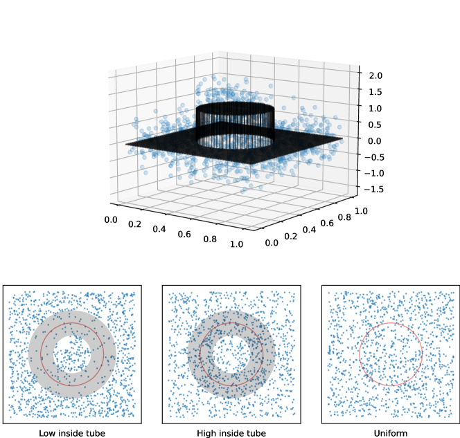
Figure 2: Illustration of the basic experimental setup used in this section. Top: the function $f_{0}$ in (27) depicted using a wireframe plot, along with $n=1274$ noisy evaluations of $f_{0}$ in blue (the noise level is set such that the signal-to-noise ratio is 1.) Bottom row: $n=1274$ samples from each of the three design distributions considered. The boundary of the set $B(x_{0},r_{0})$ is denoted in red, and the annulus $A$ is shaded in translucent gray.

We also consider three choices for the distribution $P$ of the design points $x_{1},\dots,x_{n}$, supported on $\Omega$.

1. “Low inside tube”: the sampling density $p$ is $0.295$ on an annulus $A$ centered at $x_{0}$ that has inner radius $r_{0}-0.1$ and outer radius $r_{0}+0.1$. (The density on $\Omega\setminus A$ is set to a constant value such that $p$ integrates to 1.)

2. “High inside tube”: the sampling density $p$ is $1.2$ on $A$ (with again a constant value chosen on $\Omega\setminus A$ such that $p$ integrates to 1.)

3. “Uniform”: the sampling distribution is uniform on $\Omega$.

We illustrate these sampling distributions empirically by drawing $n=1274$ observations from each and plotting them on the lower set of plots in Figure 2. We note that the “high” density value of $1.2$ for the “high inside tube” sampling distribution yields an empirical distribution that—by eye—is indistinguishable from the empirical distribution formed from uniformly drawn samples. However, as we will soon see, this departure from uniform is nonetheless large enough that the large sample behavior of the TV functionals on Voronoi adjacency, $\varepsilon$-neighborhood, and $k$-nearest neighbor graphs admit discernable differences.

4.2 Total variation estimation

We examine the of use of the Voronoi adjacency, $k$-nearest neighbor, and $\varepsilon$-neighborhood graphs, built from a random sample of design points, to estimate the total variation of the function $f_{0}$ in (27). To be clear, here we compute (using the notation (23) introduced in the asymptotic limits section):

$$\operatorname{\mathrm{DTV}}\Big{(}f_{0}(x_{1:n});w\Big{)}=\sum_{\{i,j\}\in E}w_{ij}|f_{0}(x_{i})-f_{0}(x_{j})|,$$

for three choices of edge weights $w$: Voronoi (12), $\varepsilon$-neighborhood (21), and kNN (22).

We let the number of design points $n$ range from $10^{2}$ to $10^{5}$, logarithmically spaced, with 20 repetitions independently drawn from each design distribution for each $n$. The $k$-nearest neighbor graph is built using $k=\lfloor C_{1}\log^{1.1}n\rfloor$, and the $\varepsilon$-neighborhood graph is built using $\varepsilon=C_{2}(\log^{1.1}n/n)^{1/2}$, where $C_{1},C_{2}$ are constants chosen such that the average degree of these graphs is roughly comparable to the average degree of the Voronoi adjacency graph (which has no tuning parameter). We note that it is possible to obtain marginally more stable results for the $k$-nearest neighbor and $\varepsilon$-neighborhood graphs by taking $C_{1},C_{2}$ to be larger, and thus making the graphs denser. These results are deferred to Appendix C, though we remark that the need to separately tune over such auxiliary parameters to obtain more stable results is a disadvantage of the kNN and $\varepsilon$-neighborhood methods (recall also the discussion in Section 2.4).

Figure 3 shows the results under the three design distributions outlined previously. For each sample size $n$ and for each graph, we plot the average discrete TV, and its standard error, with respect to the 20 repetitions. We additionally plot the limiting asymptotic values predicted by the theory—recall (24), (25), (26)—as horizontal lines. Generally, we can see that the discrete TV, as measured by each of the three graphs, approaches its corresponding asymptotic limit. The standard error bars for the Voronoi graph tend to be the narrowest, whereas those for the kNN and $\varepsilon$-neighborhood graphs are generally wider. In the rightmost plot, showing the results under uniform sampling, the asymptotic limits of the discrete TV for the three methods match, since the density weighting is nullified by the uniform distribution.

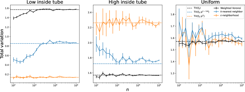
Figure 3: Results from the TV estimation experiment (“weighted Voronoi” refers to the usual Voronoi adjacency graph, with weights in (12), and is used to distinguish it from the Voronoi adjacency graph with unit edge weights, which will appear in later experiments). We see that the discrete TV as measured by each graph converges to its asymptotic limit, drawn as a dashed horizontal line, as $n$ grows (note that the $x$-axis is on a log scale).

To give a qualitative sense of their differences, Figure 4 displays the graphs from each of the methods for a draw of $n=1274$ samples under each sampling distribution. Note that the Voronoi adjacency and kNN graphs are connected (this is always the case for the former), whereas this is not true of the $\varepsilon$-neighborhood graph (recall Section 2.4), with the most noticable contrast being in the “low inside tube” sampling model. This relates to the notion that the Voronoi and kNN graphs effectively use an adaptive local bandwidth, versus the fixed bandwidth used by the $\varepsilon$-neighborhood graph. Comparing the former two (Voronoi and kNN graphs), we also see that there are fewer “holes” in the Voronoi graph as it has the quality that it seeks neighbors “in each direction” for each design point.

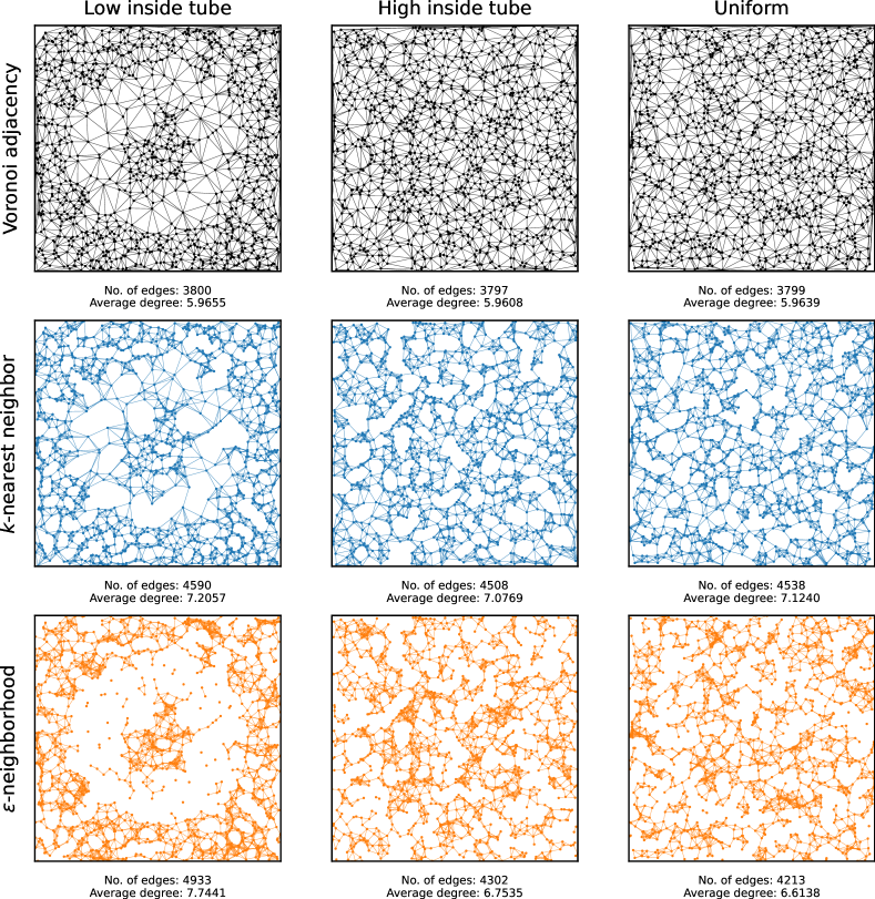
Figure 4: Visualization of the Voronoi, kNN, and $\varepsilon$-neighborhood graphs for a sample of $n=1274$ design points from each of the three sampling distributions considered. We see qualitatively very different behaviors in these three graph models, and we can also intuit the different asymptotic limits of their discrete TV functionals; for example, the strong dependence of the $\varepsilon$-neighborhood graph on the sampling density is quite noticeable in the “low inside tube” setting (bottom left plot).

4.3 Regression function estimation

Next we study the use of discrete TV from the Voronoi, $k$-nearest neighbor, and $\varepsilon$-neighborhood graphs as a penalty in a nonparametric regression estimator. In other words, given noisy observations as in (1) of the function $f_{0}$ in (27), we solve the graph TV denoising problem (14) with penalty operator $D$ equal to the edge incidence matrix corresponding to the Voronoi (12), $\varepsilon$-neighborhood (21), and kNN (22) graphs.

We fix $n=1274$, and draw each $z_{i}\sim N(0,\sigma^{2})$, where the noise level $\sigma^{2}>0$ is chosen so that the signal-to-noise ratio, defined as

$$\mathrm{SNR}=\frac{\mathrm{Var}(f_{0}(x_{i}))}{\sigma^{2}},$$

is equal to 1. (Here $\mathrm{Var}(f_{0}(x_{i}))$ denotes the variance of $f_{0}(x_{i})$ with respect to the randomness from drawing $x_{i}\sim P$.) Each graph TV denoising estimator is fit over a range of values for the tuning parameter $\lambda$, and at value of $\lambda$ we record the $L^{2}(P_{n})$ mean squared error

$$\frac{1}{n}\sum_{i=1}^{n}\big{(}\hat{f}(x_{i})-f_{0}(x_{i})\big{)}^{2}.$$

Figure 5 shows the average of this $L^{2}(P_{n})$ error, along with its standard error, across the 20 repetitions. The $x$-axis is parametrized by an estimated degrees of freedom for each $\lambda$ value, to place the methods on common footing—that is, recalling the general formula in (19) for any TV denoising estimator, we convert each value of $\lambda$ to the average number of resulting connected components over the 20 repetitions.

The results of Figure 5 broadly align with the expectations set forth at the end of Section 3: the density-weighted methods (using kNN and $\varepsilon$-neighborhood graphs) perform better when the irregularity is concentrated in a low density area (“low inside tube”), and the density-free method (the Voronoigram) does better when the irregularity is concentrated in a high density area (“high inside tube”). We also observe that across all settings, the best performing estimator tends to be the most parsimonious—the one that consumes the fewest degrees of freedom when optimally tuned.

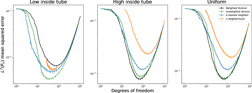
Figure 5: Results from the function estimation experiment (“weighted Voronoi” refers to the usual Voronoi graph and “unweighted Voronoi” the graph with the same edge structure but unit edge weights). We see that the density-weighted methods—TV denoising over the kNN and $\varepsilon$-neighborhood graphs—generally do better in the “low inside tube” setting, where the irregularity in $f_{0}$ is concentrated in a low density region of the design distribution. Conversely, density-free method—TV denoising on the Voronoi graph, also known as the Voronoigram—does better in the “high inside tube” scenario, where irregularity is concentrated in a high density region. Lastly, TV denoising on the unweighted Voronoi graph does very well in each scenario.

In the “low inside tube” setting (leftmost panel of Figure 5), we see that $\varepsilon$-neighborhood graph total variation does worse than its kNN counterpart, even though we would have expected the former to outperform the latter (because it weights the density more heavily; cf. (25) and (26)). The poor performance of TV denoising over the $\varepsilon$-neighborhood graph may be ascribed to the large number of disconnected points (see Figures 4 and 6), whose fitted values it cannot regularize. These disconnected points are also why the minimal degrees of freedom obtained this estimator (as $\lambda\rightarrow\infty$) is relatively large compared to kNN TV denoising and the Voronoigram, across all three settings. In Appendix C, we conduct sensitivity analysis where we grow the $\varepsilon$-neighborhood and kNN graphs more densely while retaining a comparable average degree (to each other). In that case, the performance of the corresponding estimators becomes comparable (the $\varepsilon$-neighborhood graph still has some disconnected points), which just emphasizes the peril of graph denoising methods which permit isolated points.

Interestingly, under the uniform sampling distribution (rightmost panel of Figure 5), where the asymptotic limits of the discrete TV functionals over the Voronoi, kNN, and $\varepsilon$-neighborhood graph are the same, we see that the Voronoigram performs best in mean squared error, which is encouraging empirical evidence in its favor.

Finally, Figure 5 also displays the error of the unweighted Voronoigram—which we use to refer to TV denoising on the unweighted Voronoi graph, obtained by setting each $w^{\mathrm{V}}_{ij}=1$ in (8). This is somewhat of a “surprise winner”: it performs close to the best in each of the sampling scenarios, and is computationally cheaper than the Voronoigram (it avoids the expensive step of computing the Voronoi edge weights, which requires surface area calculations). We lack an asymptotic characterization for discrete TV on the unweighted Voronoi graph, so we cannot provide a strong a priori explanation for the favorable performance of the unweighted Voronoigram over our experimental suite. Nonetheless, in view of the example adjacency graphs in Figure 4, we hypothesize that its favorable performance is at least in part due to the adaptive local bandwidth that is inherent to the Voronoi graph, which seeks neighbors “in each direction” while avoiding edge crossings. Moreover, in Section 5 we show that the unweighted Voronoigram shares the property of minimax rate optimality (for estimating functions bounded in TV and $L^{\infty}$), further strengthening its case.

4.4 Extrapolation: from fitted values to functions

As the last part of our experimental investigations, we consider extrapolating the graph TV denoising estimators, which represent a sequence of fitted values at the design points: $\hat{f}(x_{i})$, $i=1,\dots,n$, to a entire fitted function: $\hat{f}(x)$, $x\in\Omega$. As discussed and motivated in Section 2.4, we use the 1NN extrapolation rule for each estimator. This is equivalently viewed as piecewise constant extrapolation over the Voronoi tessellation.

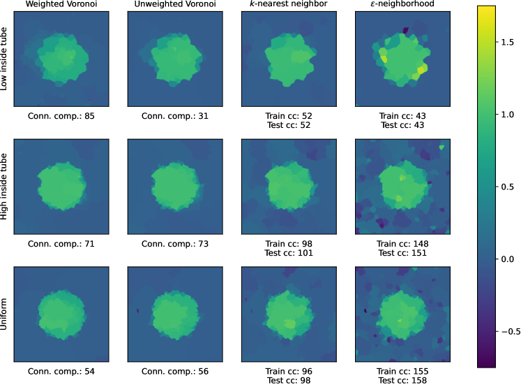
Figure 6: Extrapolants from graph TV denoising estimates, using 1NN extrapolation. We can see several qualitative differences, for example, the issues posed by isolated points in the $\varepsilon$-neighborhood graph. We also note that the number of connected components in the graph used to learn the estimator (which gives an unbiased estimate of its degrees of freedom) is guaranteed to match the number of connected components in the extrapolant only for the Voronoi methods.

Figure 6 plots the extrapolants for each TV denoising estimator, fitted over a particular sample of $n=1274$ points from each design distribution. In each case, the estimator was tuned to have optimal mean squared error (cf. Figure 5). From these visualizations, we are able to clearly understand where certain estimators struggle; for example, we can see the effect of isolated components in the $\varepsilon$-neighborhood graph in the “low inside tube” setting, and to a lesser extent in the “high inside tube” and uniform sampling settings too. As for the Voronoigram, we previously observed (cf. Figure 5 again) that it struggles in the “low inside tube” setting due to the large weights placed on edges crossing the annulus, and in the upper left plot of Figure 6 we see “patchiness” around the annulus, where large jumps are heavily penalized, rather than sharper jumps made by other estimators (including its unweighted sibling). This is underscored by the large number of connected components in the Voronoigram versus others in the “low inside tube” setting.

Lastly, because the partition induced by the 1NN extrapolation rule is exactly the Voronoi diagram, we note that the number of connected components on the training set $\{x_{1},\dots,x_{n}\}$—as measured by connectedness of the fitted values $\hat{f}(x_{1}),\dots,\hat{f}(x_{n})$ over the Voronoi graph—always matches the number of connected components on the test set $\Omega$—as measured by connectedness of the extrapolant $\hat{f}$ over the domain $\Omega$. This is not true of TV denoising over the kNN and $\varepsilon$-neighborhood graphs, where we can see a mismatch between connectedness pre- and post-extrapolation.

5 Estimation theory for BV classes

In this section, we analyze error rates for estimating $f_{0}$ given data as in (1), under the assumption that $f_{0}$ has bounded total variation. Thus, of central interest will be a (seminorm) ball in the BV space, which we denote by

$$\operatorname{\mathrm{BV}}(L)=\{f\in L^{1}(\Omega):\operatorname{\mathrm{TV}}(f)\leq L\}.$$

For simplicity, here and often throughout this section, we suppress the dependence on the domain $\Omega$ when referring to various function classes of interest. We use $P$ for the design distribution, and we will primarily be interested in error in the $L^{2}(P)$ norm, defined as

$$\|\hat{f}-f_{0}\|_{L^{2}(P)}^{2}=\int\big{(}\hat{f}(x)-f_{0}(x)\big{)}^{2}\,dP(x).$$

We also use $P_{n}$ for the empirical distribution of sample $x_{1},\dots,x_{n}$ of design points, and we will also be concerned with error in the $L^{2}(P_{n})$ norm, defined as

$$\|\hat{f}-f_{0}\|_{L^{2}(P_{n})}^{2}=\frac{1}{n}\sum_{i=1}^{n}\big{(}\hat{f}(x)-f_{0}(x)\big{)}^{2}.$$

We will generally use the terms “error” and “risk” interchangeably. Finally, we will consider the following assumptions, which we refer to as the standard assumptions.

• The design points $x_{i}$, $i=1,\dots,n$, are i.i.d. from a distribution $P$ satisfying Assumption Assumption A1.

• The response points $y_{i}$, $i=1,\dots,n$, follow (1), with i.i.d. errors $z_{i}\sim N(0,\sigma^{2})$, $i=1,\dots,n$.

• The dimension satisfies $d\geq 2$ and remains fixed as $n\to\infty$.

Note that under Assumption Assumption A1, asymptotic statements about $L^{2}(P)$ and $L^{2}(\mu)$ errors are equivalent, with $\mu$ denoting Lebesgue measure (the uniform distribution) on $\Omega$, since it holds that $p_{\mathrm{min}}\|g\|_{L^{2}(\mu)}^{2}\leq\|g\|_{L^{2}(P)}^{2}\leq p_{\mathrm{max}}\|g\|_{L^{2}(\mu)}^{2}$ for any function $g$.

5.1 Impossibility result without $L^{\infty}$ boundedness

A basic issue to explain at the outset is that, when $d\geq 2$, consistent estimation over the BV class $\operatorname{\mathrm{BV}}(L)$ is impossible in $L^{2}(P)$ risk. This is in stark contrast to the univariate setting, $d=1$, in which TV-penalized least squares (Mammen and van de Geer, 1997; Sadhanala and Tibshirani, 2019), and various other estimators, offer consistency.

One way to see this is through the fact that $\operatorname{\mathrm{BV}}(\Omega)$ does not compactly embed into $L^{2}(\Omega)$ for $d\geq 2$, which implies that $L^{2}$ estimation over $\operatorname{\mathrm{BV}}(L)$ is impossible (see Section 5.5 of Johnstone (2015) for a discussion of this phenomenon in the Gaussian sequence model). We now state this impossibility result and provide a more constructive proof, which sheds more light on the nature of the problem.

Proposition 2.

Under the standard assumptions, there exists a constant $c>0$ (not depending on $n$) such that

$$\inf_{\hat{f}}\sup_{f_{0}\in\operatorname{\mathrm{BV}}(1)\cap L^{2}(\Omega)}\mathbb{E}\|\hat{f}-f_{0}\|_{L^{2}(P)}^{2}\geq c>0,$$

where the infimum is taken over all estimators $\hat{f}$ that are measurable functions of the data $(x_{i},y_{i})$, $i=1,\dots,n$.

Proof.

As explained above, under Assumption Assumption A1 we may equivalently study $L^{2}(\mu)$ risk, which we do henceforth in this proof. We simply denote $\|\cdot\|_{L^{2}}=\|\cdot\|_{L^{2}(\mu)}$. Consider the two-point hypothesis testing problem of distinguishing

$$H_{0}:f^{\star}_{0}=0\quad\text{versus}\quad H_{1}:f^{\star}_{1}=\frac{\epsilon^{-d/2}}{2d}\cdot 1_{(0,\epsilon)^{d}},$$

where $0<\epsilon<1$. By construction, $f\in L^{2}(\Omega)$ and $\operatorname{\mathrm{TV}}(f)\leq 1$ for each of $f=f^{\star}_{0}$ and $f=f^{\star}_{1}$. Additionally, we have $\|f^{\star}_{0}-f^{\star}_{1}\|_{L^{2}}=\frac{1}{2d}$. It follows from a standard reduction that

$$\inf_{\hat{f}}\sup_{f_{0}\in\operatorname{\mathrm{BV}}(1)\cap L^{2}(\Omega)}\mathbb{E}\|\hat{f}-f_{0}\|_{L^{2}} \geq\inf_{\hat{f}}\sup_{f_{0}\in\{f^{\star}_{0},f^{\star}_{1}\}}\mathbb{E}\|\hat{f}-f_{0}\|_{L^{2}}$$

$$\geq\inf_{\psi}\Big{(}\mathbb{P}_{H_{0}}(\psi=1)+\mathbb{P}_{H_{1}}(\psi=0)\Big{)},$$ (28)

where the infimum in the rightmost expression is over all measurable tests $\psi$. Now, conditional on the event

$$\mathcal{E}=\{x_{i}\not\in(0,\epsilon)^{d},\,i=1,\dots,n\},$$

the distributions are the same under null and alternative hypotheses, $\mathbb{P}_{H_{0}}(\cdot|\mathcal{E})=\mathbb{P}_{H_{1}}(\cdot|\mathcal{E})$. Additionally, note that we have $\mathbb{P}(\mathcal{E})\geq(1-p_{\mathrm{max}}\epsilon^{d})^{n}$ under Assumption Assumption A1. Consequently, for any test $\psi$,

$$\mathbb{P}_{H_{1}}(\psi=1) =\mathbb{P}_{H_{1}}(\psi=1|\mathcal{E})\mathbb{P}(\mathcal{E})+\mathbb{P}_{H_{1}}(\psi=1|\mathcal{E}^{c})\mathbb{P}(\mathcal{E}^{c})$$

$$\leq\mathbb{P}_{H_{1}}(\psi=1)+1-(1-p_{\mathrm{max}}\epsilon^{d})^{n}$$

$$=\mathbb{P}_{H_{0}}(\psi=1)+1-(1-p_{\mathrm{max}}\epsilon^{d}).$$

In other words, just rearranging the above, we have shown that

$$\mathbb{P}_{H_{0}}(\psi=1)+\mathbb{P}_{H_{1}}(\psi=0)\geq(1-p_{\mathrm{max}}\epsilon^{d}).$$

Taking $\epsilon\to 0$, and plugging this back into (28), establishes the desired result. ∎

The proof of Proposition 2 reveals one reason why consistent estimation over $\operatorname{\mathrm{BV}}(L)$ is not possible: when $d\geq 2$, functions of bounded variation can have “spikes” of arbitrarily small width but large height, which cannot be witnessed by any finite number of samples. (We note that this has nothing to do with noise in the response, and the proposition still applies in the noiseless case with $\sigma=0$.) This motivates a solution: in the remainder of this section, we will rule out such functions by additionally assuming that $f_{0}$ is bounded in $L^{\infty}$.

5.2 Minimax error: upper and lower bounds

Henceforth we assume that $f_{0}$ has bounded TV and has bounded $L^{\infty}$ norm, that is, we consider the class

$$\operatorname{\mathrm{BV}}_{\infty}(L,M)=\{f\in L^{1}(\Omega):\operatorname{\mathrm{TV}}(f)\leq L,\,\|f\|_{L^{\infty}}\leq M\}.$$

Here $\|\cdot\|_{L^{\infty}}=\|\cdot\|_{L^{\infty}(\Omega)}$ is the essential supremum norm on $\Omega$. Perhaps surprisingly, additionally assuming that $f_{0}$ is bounded in $L^{\infty}$ dramatically improves prospects for estimation. The following theorem shows that two different and simple modifications of the Voronoigram, appropriately tuned, each achieve a $n^{-1/d}$ rate of convergence in its sup risk over $\operatorname{\mathrm{BV}}_{\infty}(L,M)$, modulo log factors.

Theorem 2.

Under the standard assumptions, consider either of the following modified Voronoigram estimators $\hat{\theta}$:

• the minimizer in the Voronoigram problem (8), once we replace each weight $w^{\mathrm{V}}_{ij}$ by a clipped version defined as $\tilde{w}^{\mathrm{V}}_{ij}=\max\{c_{0}n^{-(d-1)/d},w^{\mathrm{V}}_{ij}\}$, for any constant $c_{0}>0$.

• the minimizer in the Voronoigram problem (8), once we replace each weight $w^{\mathrm{V}}_{ij}$ by 1.

Let $\lambda=c\sigma\tau_{n}(\log n)^{1/2+\alpha}$ for any $\alpha>1$ and a constant $c>0$, where $\tau_{n}=n^{(d-1)/d}$ for the clipped weights estimator and $\tau_{n}=1$ for the unit weights estimator. There exists another constant $C>0$ such that for all sufficiently large $n$ and $f_{0}\in\operatorname{\mathrm{BV}}_{\infty}(L,M)$, the estimated function $\hat{f}=\sum_{i=1}^{n}\hat{\theta}_{i}\cdot 1_{V_{i}}$ (which is piecewise constant over the Voronoi diagram) satisfies

$$\mathbb{E}\|\hat{f}-f_{0}\|_{L^{2}(P)}^{2}\leq C\bigg{(}\frac{\sigma L(\log n)^{5/2+\alpha+1/d}}{n^{1/d}}+\frac{(\log n)^{1+\alpha}}{n}+\frac{LM(\log n)^{1+1/d}}{n^{1/d}}\bigg{)}.$$ (29)

We now certify that this upper bound is tight, up to log factors, by providing a complementary lower bound.

Theorem 3.

Under the standard assumptions, provided that $n,L,M$ satisfy $c_{0}(M^{2}n)^{-\frac{(d-1)}{d}}\leq L\leq C_{0}(M^{2}n)^{1/d}$ for constants $C_{0}>c_{0}>0$, the minimax risk satisfies

$$\inf_{\hat{f}}\sup_{f_{0}\in\operatorname{\mathrm{BV}}_{\infty}(L,M)}\mathbb{E}\|\hat{f}-f_{0}\|_{L^{2}(P)}^{2}\geq CLM(M^{2}n)^{-1/d},$$ (30)

for another constant $C>0$, where the infimum is taken over all estimators $\hat{f}$ that are measurable functions of the data $(x_{i},y_{i})$, $i=1,\dots,n$.

Taken together, Theorems 2 and 3 establish that the minimax rate of convergence over $\operatorname{\mathrm{BV}}_{\infty}(1,1)$ is $n^{-1/d}$, modulo log factors. Further, after subjecting it to minor modifications—either clipping small edge weights, or setting all edge weights to unity (the latter being particularly desirable from a computational point of view)—the Voronoigram is minimax rate optimal, again up to log factors.

The proof of the lower bound (30) is Theorem 3 is fairly standard and can be found in Appendix D. The proof of the upper bound (29) in Theorem 2 is much more involved, and the key steps are described over Sections 5.3 and 5.4 (with the details deferred to Appendix D). Before moving on to key parts of the analysis, we make several remarks.

Remark 4.

It is not clear to us whether clipping small weights in the Voronoigram penalty as we do in Theorem 2 (via $\tilde{w}^{\mathrm{V}}_{ij}=\max\{c_{0}n^{-(d-1)/d},w^{\mathrm{V}}_{ij}\}$) is actually needed, or whether the unmodified estimator (8) itself attains the same or a similar upper bound, as in (29). In particular, it may be that under Assumption Assumption A1, the surface area of the boundaries of Voronoi cells (defining the weights) are already lower bounded in rate by $n^{-(d-1)/d}$, with high probability; however this is presently unclear to us.

Remark 5.

The design points must be random in order to have nontrivial rates of convergence in our problem setting. If $x_{1},\dots,x_{n}$ were instead fixed, then for $d\geq 2$ and any $n$ it is possible to construct $f_{0}\in\operatorname{\mathrm{BV}}_{\infty}(1,1)$ with $f_{0}(x_{i})=0$, $i=1,\dots,n$ and (say) $\|f\|_{L^{2}}=1/2$. Standard arguments based on reducing to a two-point hypothesis testing problem (as in the proof of Proposition 2) reveal that the minimax rate in $L^{2}$ is trivially lower bounded by a constant, rendering consistent estimation impossible once again.

This is completely different from the situation for $d=1$, where the minimax risks under fixed and random design models for TV bounded functions are basically equivalent. Fundamentally, this is because for $d\geq 2$ the space $\operatorname{\mathrm{BV}}(\Omega)$ does not compactly embed into $C^{0}(\Omega)$, the space of continuous functions (whereas for $d=1$, all functions in $\operatorname{\mathrm{BV}}(\Omega)$ possess at least an approximate form of continuity). Note carefully that this is a different issue than the failure of $\operatorname{\mathrm{BV}}(\Omega)$ to compactly embed into $L^{2}(\Omega)$, and that it is not fixed by intersecting a TV ball with an $L^{\infty}$ ball.

Remark 6.

We can generalize the definition of total variation in (2), by generalizing the norm we use to constrain the “test” function $\phi$ to an arbitrary norm $\|\cdot\|$ on $\mathbb{R}^{d}$. (See (S.1) in the appendix.) The original definition in (2) uses the $\ell_{2}$ norm, $\|\cdot\|=\|\cdot\|_{2}$. What would minimax rates look if we used a different choice of norm to define TV? Suppose that we use an $\ell_{p}$ norm, for any $p\geq 1$; that is, suppose we take $\|\cdot\|=\|\cdot\|_{p}$ as the norm to constrain the “test” functions in the supremum. Then under this change, the minimax rate will still remain $n^{-1/d}$, just as in Theorems 2 and 3. This is simply due to the fact that $\ell_{p}$ norms are equivalent on $\mathbb{R}^{d}$ (thus a unit ball in the TV-$\ell_{p}$ seminorm will be sandwiched in between two balls in TV-$\ell_{2}$ seminorm of constant radii).

Remark 7.

The minimax rate for estimating a Lipschitz function, that is, the minimax rate over the class

$$\mathrm{Lip}(L)=\{f:\Omega\to\mathbb{R}\,:\,|f(x)-f(z)|\leq L\|x-z\|_{2}\;\text{for all $x,z\in\Omega$}\},$$

is $n^{-2/(2+d)}$ in squared $L^{2}$ risk, for constant $L>0$ (not growing with $n$); see, e.g., Stone (1982). When $d=2$, this is equal to $n^{-1/2}$, implying that the minimax rates for estimation over $\mathrm{Lip}(1)$ and $\operatorname{\mathrm{BV}}_{\infty}(1,1)$ match (up to log factors). This is despite the fact that $\mathrm{Lip}(1)$ is a strict subset of $\operatorname{\mathrm{BV}}_{\infty}(1,1)$, with the latter containing far more diverse functions, such as those with sharp discontinuities (indicator functions being a prime example). When $d\geq 3$, we can see that the minimax rates drift apart, with that for $\operatorname{\mathrm{BV}}_{\infty}(1,1)$ being slower than $\mathrm{Lip}(1)$, increasingly so for larger $d$.

Remark 8.

A related point worthy of discussion is about what types of estimators can attain optimal rates over $\mathrm{Lip}(1)$ and $\operatorname{\mathrm{BV}}_{\infty}(1,1)$. For $\mathrm{Lip}(1)$, various linear smoothers are known to be optimal, which describes an estimator $\hat{f}$ of the form $\hat{f}(x)=w(x)^{\mathsf{T}}y$ for a weight function $w:\Omega\to\mathbb{R}^{n}$ (the weight function can depend on the design points but not on the response vector $y$). This includes kNN regression and kernel smoothing, among many other traditional methods. For $\operatorname{\mathrm{BV}}_{\infty}(1,1)$, meanwhile, we have shown that the (modified) Voronoigram estimator is optimal (modulo log factors), which is highly nonlinear as a function of $y$. All other examples of minimax rate optimal estimators that we provide in Section 5.5 are nonlinear in $y$ as well. In fact, we conjecture that no linear smoother can achieve the minimax rate over $\operatorname{\mathrm{BV}}_{\infty}(1,1)$. There is very strong precedence for this, both from the univariate case (Donoho and Johnstone, 1998) and from the multivariate lattice case (Sadhanala et al., 2016). We leave a minimax linear analysis over $\operatorname{\mathrm{BV}}_{\infty}(1,1)$ to future work.

Remark 9.

Lastly, we comment on the relationship to the results obtained in Padilla et al. (2020). These authors study TV denoising over the $\varepsilon$-neighborhood and kNN graphs; our analysis also extends to cover these estimators, as shown in Section 5.5. They obtain a comparable squared $L^{2}$ error rate of $n^{-1/d}$, under a related but different set of assumptions. In one way, their assumptions are more restrictive than ours, because they require conditions on $f_{0}$ that are stronger than TV and $L^{\infty}$ boundedness: they require it to satisfy an additional assumption that generalizes piecewise Lipschitz continuity, but is difficult to assess, in terms of understanding precisely which functions have this property. (They also directly consider functions that are piecewise Lipschitz, but this assumption is so strong that they are able to remove the BV assumption entirely and attain the same error rates.)

In another way, the results in Padilla et al. (2020) go beyond ours, since they accomodate the case when the design points lie on a manifold, in which case their estimation rates are driven by the intrinsic (not ambient) dimension. Such manifold adaptivity is possible due to strong existing results on the properties of the $\varepsilon$-neighborhood and kNN graphs in the manifold setting. Is is unclear to us whether the Voronoi graph has similar properties. This would be an interesting topic for future work.

5.3 Analysis of the Voronoigram: $L^{2}(P_{n})$ risk

We outline the analysis of the Voronoigram. The analysis proceeds in three parts. First, we bound the $L^{2}(P_{n})$ risk of the Voronoigram in terms of the discrete TV of the underlying signal over the Voronoi graph. Second, we bound this discrete TV in terms of the continuum TV of the underlying function. This is presented in Lemmas 1 and 2, respectively. The third step is to bound the $L^{2}(P)$ risk after extrapolation (to a piecewise constant function on the Voronoi diagram), which is presented in Lemma 3 in the next subsection. All proofs are deferred until Appendix D.

For the first part, we effectively reduce the discrete analysis of the Voronoigram—in which we seek to upper bound its $L^{2}(P_{n})$ risk in terms of its discrete TV—to the analysis of TV denoising on a grid. Analyzing this estimator over a grid is desirable because a grid graph has nice spectral properties (cf. the analyses in Wang et al. (2016); Hutter and Rigollet (2016); Sadhanala et al. (2016, 2017, 2021) which all leverage such properties). In the language of functional analysis, the core idea here is an embedding between the spaces defined by the discrete TV operators with respect to one graph $G$ and another $G^{\prime}$, of the form

$$\|D(G^{\prime})\,\theta\|_{1}\leq C_{n}\|D(G)\,\theta\|_{1},\quad\text{for all $\theta\in\mathbb{R}^{n}$},$$

where $D(G),D(G^{\prime})$ denote their respective edge incidence operators. This approach was pioneered in Padilla et al. (2018), who used it to study error rates for TV denoising in quite a general context. It is also the key behind the analysis of TV denoising on the $\varepsilon$-neighborhood and kNN graph in Padilla et al. (2020), who also perform a reduction to a grid graph. The next lemma, inspired by this work, shows that the analogous reduction is available for the Voronoi graph.

Lemma 1.

Under the standard assumptions, consider either of the two modified Voronoi weighting schemes defined in Theorem 2:

• $\tilde{w}^{\mathrm{V}}_{ij}=\max\{c_{0}n^{-(d-1)/d},w^{\mathrm{V}}_{ij}\}$ for each $i,j$ such that $w^{\mathrm{V}}_{i,j}>0$;

• $\check{w}^{\mathrm{V}}_{ij}=1$ for each $i,j$ such that $w^{\mathrm{V}}_{i,j}>0$.

Let $D$ denote the edge incidence operator corresponding to the modified graph, and $\hat{\theta}$ the solution in (14) (equivalently, it is the solution in (8) after substituting in the modified weights). Then there exists a matrix $D^{\prime}$, that can be viewed as a suitably modified edge incidence operator corresponding to a $d$-dimensional grid graph, such that

$$\|D^{\prime}\theta\|_{1}\leq C_{n}\tau_{n}\|D\theta\|_{1},\quad\text{for all $\theta\in\mathbb{R}^{n}$},$$ (31)

with probability at least $1-3/n^{4}$ (with respect to the distribution of design points), where $C_{n}>0$ grows polylogarithmically in $n$ and $\tau_{n}$ is the scaling factor defined in Theorem 2. Further, letting $\lambda=c\sigma\tau_{n}(\log n)^{1/2+\alpha}$ for any $\alpha>1$ and a constant $c>0$, there exists another constant $C>0$ such that for all sufficiently large $n$ and $f_{0}\in\operatorname{\mathrm{BV}}(\Omega)$,

$$\mathbb{E}\bigg{[}\frac{1}{n}\|\hat{\theta}-\theta_{0}\|_{2}^{2}\bigg{]}\leq C\bigg{(}\frac{\sigma\tau_{n}(\log n)^{1/2+\alpha}}{n}\mathbb{E}\|D\theta_{0}\|_{1}+\frac{(\log n)^{\alpha}}{n}\bigg{)},$$ (32)

where we denote $\theta_{0}=(f_{0}(x_{1}),\dots,f_{0}(x_{n}))\in\mathbb{R}^{n}$.

Notice that, in equivalent notation, we can write the left-hand side in (32) as $n^{-1}\|\hat{\theta}-\theta_{0}\|_{2}^{2}=\|\hat{f}-f_{0}\|_{L^{2}(P_{n})}^{2}$, for the estimated function satisfying $\hat{f}(x_{i})=\hat{\theta}_{i}$, $i=1,\dots,n$; and for the $\ell_{1}$ term on the right-hand side in (32) we can write $\|D\theta_{0}\|_{1}=\operatorname{\mathrm{DTV}}(f_{0}(x_{1:n});\,w)$ for suitable edge weights $w$—either of the two choices defined in bullet points at the start of the theorem—over the Voronoi graph.

As we can see, the $L^{2}(P_{n})$ risk of the Voronoigram depends on the discrete TV of the true signal over the Voronoi graph. A natural question to ask, then, is whether a function bounded in continuum TV is also bounded in discrete TV, when the latter is measured using the Voronoi graph. Our next result answers this in the affirmative. It is inspired by analogous results developed in Green et al. (2021a, b) for Sobolev functionals.

Lemma 2.

Under Assumption Assumption A1, there exists a constant $C>0$ such that for all sufficiently large $n$ and $f_{0}\in\operatorname{\mathrm{BV}}(\Omega)$, with $w$ denoting either of the two choices of edge weights given at the start of Lemma 1,

$$\mathbb{E}\Big{[}\operatorname{\mathrm{DTV}}\Big{(}f_{0}(x_{1:n});\,w\Big{)}\Big{]}\leq C\bar{\tau}_{n}(\log n)^{1+1/d}\operatorname{\mathrm{TV}}(f_{0}),$$ (33)

where $\bar{\tau}_{n}=n^{(d-1)/d}/\tau_{n}$ (which is 1 for the clipped weights estimator and $n^{(d-1)/d}$ for the unit weights estimator).

Lemmas 1 and 2 may be combined to yield the following result, which is the $L^{2}(P_{n})$ analog of Theorem 2.

Corollary 1.

Under the standard assumptions, for either of the two modified Voronoigram estimators from Theorem 2, letting $\lambda=c\sigma\tau_{n}(\log n)^{1/2+\alpha}$ for any $\alpha>1$ and a constant $c>0$, there exists another constant $C>0$ such that for all sufficiently large $n$ and $f_{0}\in\operatorname{\mathrm{BV}}(L)$,

$$\mathbb{E}\|\hat{f}-f_{0}\|_{L^{2}(P_{n})}^{2}\leq C\bigg{(}\frac{\sigma L(\log n)^{3/2+\alpha+1/d}}{n^{1/d}}+\frac{(\log n)^{\alpha}}{n}\bigg{)}.$$ (34)

Note that for a constant $L$ (not growing with $n$), the $L^{2}(P_{n})$ bound in (34) converges at the rate $n^{-1/d}$, up to log factors. Interestingly, this $L^{2}(P_{n})$ guarantee does not require $f_{0}$ to be bounded in $L^{\infty}$, which we saw was required for consistent estimation in $L^{2}(P)$ error. Next, we will turn to an $L^{2}(P)$ upper bound, which does require $L^{\infty}$ boundedness on $f_{0}$. That this is not needed for $L^{2}(P_{n})$ consistency is intuitive (at least in hindsight): recall that we saw from the proof of Proposition 2 that inconsistency in $L^{2}(P)$ occurred due to tall spikes with vanishing width but non-vanishing $L^{2}$ norm, which could not be witnessed by a finite number of samples. To the $L^{2}(P_{n})$ norm, which only measures error at locations witnessed by the sample points, these pathologies are irrelevant.

5.4 Analysis of the Voronoigram: $L^{2}(P)$ risk

To close the loop, we derive bounds on the $L^{2}(P)$ risk of the Voronoigram via the $L^{2}(P_{n})$ bounds just established. For this, we need to consider the behavior of the Voronoigram estimator off of the design points. Recall that an equivalent interpretation of the Voronoigram fitted function, $\hat{f}=\sum_{i=1}^{n}\hat{f}(x_{i})\cdot 1_{V_{i}}$, is that it is given by 1-nearest-neighbor (1NN) extrapolation, applied to $(x_{i},\hat{f}(x_{i}))$, $i=1,\dots,n$. Our approach here is to define an analogous 1NN extrapolant $\bar{f}_{0}$ to $(x_{i},f_{0}(x_{i}))$, $i=1,\dots,n$, and then use the triangle inequality, along with the fact that $\hat{f},\bar{f}_{0}$ are piecewise constant on the Voronoi diagram, to argue that

$$\|\hat{f}-f_{0}\|_{L^{2}(P)}^{2} \leq 2\|\hat{f}-\bar{f}_{0}\|_{L^{2}(P)}^{2}+2\|\bar{f}_{0}-f_{0}\|_{L^{2}(P)}^{2}$$

$$=2\sum_{i=1}^{n}\big{(}\textstyle{\int}_{V_{i}}1dP\big{)}\big{(}\hat{f}(x_{i})-f_{0}(x_{i})\big{)}^{2}+2\|\bar{f}_{0}-f_{0}\|_{L^{2}(P)}^{2}$$

$$\leq\underbrace{2p_{\mathrm{max}}n\cdot\bigg{(}\max_{i=1,\dots,n}\mu(V_{i})\bigg{)}}_{K_{n}}\|\hat{f}-f_{0}\|_{L^{2}(P_{n})}^{2}+2\|\bar{f}_{0}-f_{0}\|_{L^{2}(P)}^{2},$$ (35)

where $\mu(V_{i})$ denotes the Lebesgue volume of $V_{i}$. The first term in (35) is the $L^{2}(P_{n})$ error multiplied by a factor $K_{n}$ that is driven by the maximum volume of a Voronoi cell, which we can show is well controlled (of order $\log n/n$) under Assumption Assumption A1. The second term is a kind of $L^{2}(P)$ approximation error from applying the 1NN extrapolation rule to evaluations of $f_{0}$ itself. When $f_{0}\in\operatorname{\mathrm{BV}}_{\infty}(L,M)$, this is also well controlled, as we show next.

Lemma 3.

Assume that $x_{1},\dots,x_{n}$ are i.i.d. from a distribution satisfying Assusmption Assumption A1. Then there is a constant $C>0$ such that for all sufficiently large $n$ and $f_{0}\in\operatorname{\mathrm{BV}}_{\infty}(L,M)$,

$$\mathbb{E}\|\bar{f}_{0}-f_{0}\|_{L^{2}(P)}^{2}\leq C\bigg{(}\frac{LM(\log n)^{1+1/d}}{n^{1/d}}\bigg{)}.$$ (36)

We make two remarks to conclude this subsection.

Remark 10.

For nonparametric regression with random design, a standard approach is to use uniform concentration results that couple the $L^{2}(P)$ and $L^{2}(P_{n})$ norms in order to obtain an error guarantee in one norm from a guarantee in the other; see, e.g., Chapter 14 of Wainwright (2019). In our setting, such an approach is not applicable—the simplest explanation being that for any $x_{1},\dots,x_{n}$, there will always exist a function $f\in\operatorname{\mathrm{BV}}_{\infty}(1,1)$ for which $\|f\|_{L^{2}(P_{n})}=0$ but $\|f\|_{L^{2}(P)}=1/2$. This is the same issue as that discussed in Remark 5.

Remark 11.

The contribution of the extrapolation risk in (36) to the overall bound in (29) is not negligible. This raises the possibility that, for this problem, extrapolation from random design points with noiseless function values can be at least as hard as $L^{2}(P_{n})$ estimation from noisy responses. This is in contrast with conventional wisdom which says that the noiseless problem is generally much easier. Of course, Lemma 3 only provides an upper bound on the extrapolation risk, without a matching lower bound. Resolving the minimax $L^{2}(P)$ error in the noiseless setting, and more broadly, studying its precise dependence on the noise level $\sigma$, is an interesting direction for future work.

5.5 Other minimax optimal estimators

Finally, we present $L^{2}(P)$ guarantees that show that other estimators can also obtain minimax optimal rates (up to log factors) for the class of functions bounded in TV and $L^{\infty}$. First, we consider TV denoising on $\varepsilon$-neighborhood and kNN graphs, using 1NN extrapolation to turn them into functions on $\Omega$. The analysis is altogether very similar to that for the Voronoigram outlined in the preceding subsections, and the details are deferred to Appendix D. A notable difference, from the perspective of methodology, is that these estimators require proper tuning in the graph construction itself.

Theorem 4.

Under the standard assumptions, consider the graph TV denoising estimator $\hat{\theta}^{\varepsilon}$ which solves problem (14) with $D=D(G^{\varepsilon})$, the edge incidence operator of the $\varepsilon$-neighborhood graph $G^{\varepsilon}$, with edge weights as in (21). Letting $\varepsilon=c_{1}((\log n)^{\alpha}/n)^{1/d}$ and $\lambda=c_{2}\sigma(\log n)^{1/2-\alpha}$ for any $\alpha>1$ and constants $c_{1},c_{2}>0$, there is a constant $C>0$ such that for all sufficiently large $n$ and $f_{0}\in\operatorname{\mathrm{BV}}_{\infty}(L,M)$, the 1NN extrapolant $\hat{f}^{\varepsilon}=\sum_{i=1}^{n}\hat{\theta}_{i}^{\varepsilon}\cdot 1_{V_{i}}$ satisfies

$$\mathbb{E}\|\hat{f}^{\varepsilon}-f_{0}\|_{L^{2}(P)}^{2}\leq C\bigg{(}\frac{\sigma L(\log n)^{3/2+\alpha/d}}{n^{1/d}}+\frac{(\log n)^{1+\alpha}}{n}+\frac{LM(\log n)^{1+1/d}}{n^{1/d}}\bigg{)}.$$ (37)

Consider instead the graph TV denoising estimator $\hat{\theta}^{k}$ which solves problem (14) with $D=D(G^{k})$, the edge incidence operator of the kNN graph $G^{k}$, with edge weights as in (22). Letting $k=c^{\prime}_{1}(\log n)^{3}$ and $\lambda=c_{2}^{\prime}\sigma(\log n)^{1/2-\alpha}$ for any $\alpha>1$ and constants $c_{1}^{\prime},c_{2}^{\prime}>0$, there is a constant $C^{\prime}>0$ such that for all sufficiently large $n$ and $f_{0}\in\operatorname{\mathrm{BV}}_{\infty}(L,M)$, the 1NN extrapolant $\hat{f}^{k}=\sum_{i=1}^{n}\hat{\theta}_{i}^{k}\cdot 1_{V_{i}}$ satisfies

$$\mathbb{E}\|\hat{f}^{k}-f_{0}\|_{L^{2}(P)}^{2}\leq C^{\prime}\bigg{(}\frac{\sigma L(\log n)^{9/2-\alpha+3/d}}{n^{1/d}}+\frac{(\log n)^{1+\alpha}}{n}+\frac{LM(\log n)^{1+1/d}}{n^{1/d}}\bigg{)}.$$ (38)

Next, and last, we consider wavelet denoising. For this we assume that the design density is uniform on $\Omega=(0,1)^{d}$. The analysis is quite different from the preceding ones, but it relies on fairly standard techniques in wavelet theory, and we defer the details to Appendix D.

Theorem 5.

Under the standard conditions, further assume that $P=\mu$, the uniform measure on $\Omega=(0,1)^{d}$. For an estimator $\hat{f}^{\mathrm{wav}}$ based on hard-thresholding Haar wavelet coefficients, there exist constants $c,C>0$ such that for all sufficiently large $n$ and $f_{0}\in\operatorname{\mathrm{BV}}_{\infty}(L,M)$, it holds that

$$\mathbb{E}\|\hat{f}^{\mathrm{wav}}-f_{0}\|_{L^{2}}^{2}\leq\frac{CLM}{n^{1/d}}+C\cdot\begin{cases}L\delta_{n}^{\ast}\max\{1,\,1/M,\,\log_{2}(M\sqrt{n})\}&d=2\\ L^{2/d}(\delta_{n}^{\ast})^{4/(2+d)}+LM(\delta_{n}^{\ast}/M)^{2/d}&d\geq 3,\end{cases}$$ (39)

where $\delta_{n}^{\ast}=(c/\sqrt{n})((\log n)^{3/2}+M(\log n)^{1/2})$.

6 Discussion

In this paper, we studied total variation as it touches on various aspects of multivariate nonparametric regression, such as discrete notions of TV based on scattered data, the use of discrete TV as a regularizer in nonparametric estimators, and estimation theory over function classes where regularity is given by (continuum) TV.

We argued that a particular formulation of discrete TV, based on the graph formed by adjacencies with respect to the Voronoi diagram of the design points $x_{1},\dots,x_{n}$, has several desirable properties when used as the regularizer in a penalized least squares context—defining an estimator we call the Voronoigram. Among these properties:

• it is user-friendly (requiring no auxiliary tuning parameter unlike other geometric graphs, such as $\varepsilon$-neighborhood or $k$-nearest-neighbor graphs);

• it tracks “pure TV” in large samples, meaning that discrete TV on the Voronoi graph converges asymptotically to continuum TV, independent of the design density (as opposed to $\varepsilon$-neighborhood or kNN graphs, which give rise to certain types of density-weighted TV in the limit);

• it achieves the minimax optimal convergence rate in $L^{2}$ error over a class of functions bounded in TV and $L^{\infty}$;

• it admits a natural duality between discrete and continuum formulations, so the fitted values $\hat{f}(x_{i})$, $i=1,\dots,n$ have exactly the same variation (as measured by discrete TV) over the design points as the fitted function $\hat{f}$ (as measured by continuum TV) over the entire domain.

The last property here is completely analogous to the discrete-continuum duality inherent in trend filtering (Tibshirani, 2014, 2022), which makes the Voronoigram a worthy successor to trend filtering for multivariate scattered data, albeit restricted to the polynomial order $k=0$ (piecewise constant estimation).

Several directions for future work have already been discussed throughout the paper. We conclude by mentioning one more: extension to the polynomial order $k=1$, i.e., adaptive piecewise linear estimation, in the multivariate scattered data setting. For this problem, we believe the estimator proposed by Koenker and Mizera (2004), defined in terms of the Delaunay tessellation (which is dual to the Voronoi diagram) of the design points, will enjoy many properties analogous to the Voronoigram, and is deserving of further study.

Appendix A Added details and proofs for Sections 1 and 2

A.1 Discussion of sampling model for BV functions

We clarify what is meant by the sampling model in (1), since, strictly speaking, each element $f\in\operatorname{\mathrm{BV}}(\Omega)$ is really an equivalence class of functions, defined only up to sets of Lebesgue measure zero. This issue is not simply a formality, and becomes a genuine problem for $d\geq 2$, as in this case the space $\operatorname{\mathrm{BV}}(\Omega)$ does not compactly embed into $C^{0}(\Omega)$, the space of continuous functions on $\Omega$ (equipped with the $L^{\infty}$ norm). A key implication of this is that the point evaluation operator is not continuous over $\operatorname{\mathrm{BV}}(\Omega)$.

In order to make sense of the evaluation map, $x\mapsto f(x)$, we will pick a representative, denoted $f^{\star}\in f$, and speak of evaluations of this representative. Our approach here is the same as that taken in Green et al. (2021a, b), who study minimax estimation of Sobolev functions in the subcritical regime (and use an analogous random design model). We let $f^{\star}$ be the precise representative, defined (Evans and Gariepy, 2015) as:

$$f^{\star}(x)=\begin{cases}\displaystyle\lim_{\epsilon\to 0}\frac{1}{\mu(B(x,\epsilon))}\int_{B(x,\epsilon)}f(z)\,dz&\text{if the limit exists}\\ 0&\text{otherwise}.\end{cases}$$

Here $\mu$ denotes Lebesgue measure and $B(x,\epsilon)$ is the ball of radius $\epsilon$ centered at $x$.

Now we explain why the particular choice of representative is not crucial, and any choice of representative would have resulted in the same interpretation of function evaluations in (1), almost surely, assuming that each $x_{i}$ is drawn from a continuous distribution on $\Omega$. Recall that for a locally integrable function $f$ on $\Omega$, we say that a given point $x\in\Omega$ is a Lebesgue point of $f$ provided that $\lim_{\epsilon\to 0}(\int_{B(x,\epsilon)}f(z)\,dz)/\mu(B(x,\epsilon))$ exists and equals $f(x)$. By the Lebesgue differentiation theorem (e.g., Theorem 1.32 of Evans and Gariepy, 2015), for any $f\in L^{1}(\Omega)$, almost every $x\in\Omega$ is a Lebesgue point of $f$. This means that each evaluation $f^{\star}(x_{i})$ of the precise representative will equal the evaluation of any member of the equivalence class, almost surely (with respect to draws of $x_{i}$). This justifies the notation $f(x_{i})$ used in the main text, for $f\in\operatorname{\mathrm{BV}}(\Omega)$ and $x_{i}$ drawn from a continuous probability distribution.

A.2 TV representation for piecewise constant functions

Here we will state and prove a more general result from which Proposition 1 will follow. First we give a more general definition of measure theoretic total variation, wherein the norm used to constrain the “test function” $\phi$ in the supremum is an arbitrary norm $\|\cdot\|$ on $\mathbb{R}^{d}$,

$$\operatorname{\mathrm{TV}}(f;\Omega,\|\cdot\|)=\sup\left\{\int_{\Omega}f(x)\operatorname{\mathrm{div}}\phi(x)\,dx:\phi\in C_{c}^{1}(\Omega;\mathbb{R}^{d}),\,\|\phi(x)\|\leq 1\;\text{for all $x\in\Omega$}\right\}.$$ (S.1)

Note that our earlier definition in (2) corresponds to the special case $\operatorname{\mathrm{TV}}(f;\Omega,\|\cdot\|_{2})$, that is, corresponds to choosing $\|\cdot\|=\|\cdot\|_{2}$ in (S.1). In the more general TV context, this special case is often called isotropic TV.

Proposition S.1.

Let $V_{1},\dots,V_{n}$ be an open partition of $\Omega$ such that each $V_{i}$ is semialgebraic. Let $f$ be of the form

$$f=\sum_{i=1}^{n}\theta_{i}\cdot 1_{V_{i}},$$

for arbitrary $\theta_{1},\dots,\theta_{n}\in\mathbb{R}$. Then, for any norm $\|\cdot\|$ and its dual norm $\|\cdot\|_{*}$ (induced by the Euclidean inner product), we have

$$\operatorname{\mathrm{TV}}(f;\Omega,\|\cdot\|)=\sum_{i,j=1}^{n}\bigg{(}\int_{\partial V_{i}\cap\partial V_{j}}\|n_{i}(t)\|_{*}\,d\mathcal{H}^{d-1}(t)\bigg{)}\cdot|\theta_{i}-\theta_{j}|,$$

where $n_{i}(t)$ is the measure theoretic unit outer normal for $V_{i}$ at a boundary point $t\in\partial V_{i}$. In particular, in the isotropic case $\|\cdot\|=\|\cdot\|_{2}$,

$$\operatorname{\mathrm{TV}}(f;\Omega,\|\cdot\|_{2})=\sum_{i,j=1}^{n}\mathcal{H}^{d-1}(\partial V_{i}\cap\partial V_{j})\cdot|\theta_{i}-\theta_{j}|.$$

Remark 12.

The condition that each $V_{i}$ is semialgebraic may to weakened to what is called “polynomially bounded boundary measure.” Namely, the proposition still holds if each map $r\mapsto\mathcal{H}^{d-1}(\partial V_{i}\cap B(0,r))$ is polynomially bounded (cf. Assumption 2.2 in Mikkelsen and Hansen, 2018). This is sufficient to guarantee a locally Lipschitz boundary (a prerequisite for the application of Gauss-Green) and to characterize the outer normals associated with the partition $V_{1},\dots,V_{n}$.

Proof.

We begin by deriving an equivalent expression of total variation of piecewise constant functions.

$$\operatorname{\mathrm{TV}}(f;\, \Omega,\lVert\cdot\rVert)$$

$$=\sup\left\{\int_{\Omega}f(x)\operatorname{\mathrm{div}}\phi(x)dx:\phi\in C_{c}^{1}(\Omega;\mathbb{R}^{d}),\lVert\phi\rVert_{*}\leq 1\;\forall x\right\}$$

$$=\sup\left\{\sum_{i=1}^{n}\int_{V_{i}}\theta_{i}\operatorname{\mathrm{div}}\phi(x)dx:\phi\in C_{c}^{1}(\Omega;\mathbb{R}^{d}),\lVert\phi\rVert_{*}\leq 1\;\forall x\right\}$$

$$=\sup\left\{\sum_{i=1}^{n}\theta_{i}\int_{\partial V_{i}}\langle\phi(t),n_{i}(t)\rangle d\mathcal{H}^{d-1}(t):\phi\in C_{c}^{1}(\Omega;\mathbb{R}^{d}),\lVert\phi\rVert_{*}\leq 1\;\forall x\right\}$$ (S.2)

$$\begin{split}&=\sup\Bigg{\{}\sum_{i,j=1}^{n}\left(\theta_{i}\int_{\partial V_{i}\cap\partial V_{j}}\langle\phi(t),n_{i}(t)\rangle d\mathcal{H}^{d-1}(t)+\theta_{j}\int_{\partial V_{i}\cap\partial V_{j}}\langle\phi(t),n_{j}(t)\rangle d\mathcal{H}^{d-1}(t)\right)\\ &\hskip 42.67912pt+\sum_{i:\bar{V}_{i}\cap\partial\Omega\neq\emptyset}\theta_{i}\underbrace{\int_{\partial V_{i}\cap\partial\Omega}\langle\phi(t),n_{i}(t)\rangle d\mathcal{H}^{d-1}(t)}_{=0\text{; ($\phi$ compactly supported)}}:\phi\in C_{c}^{1}(\Omega;\mathbb{R}^{d}),\lVert\phi\rVert_{*}\leq 1\;\forall t\Bigg{\}}\end{split}$$ (S.3)

$$=\sup\Bigg{\{}\sum_{i,j=1}^{n}\int_{\partial V_{i}\cap\partial V_{j}}(\theta_{i}-\theta_{j})\langle\phi(t),n_{i}(t)\rangle d\mathcal{H}^{d-1}(t):\phi\in C_{c}^{1}(\Omega;\mathbb{R}^{d}),\lVert\phi\rVert_{*}\leq 1\;\forall t\Bigg{\}}$$ (S.4)

we obtain (S.2) by applying the Gauss-Green Theorem (Evans and Gariepy, 2015, Theorem 5.16); (S.3) by observing that when the boundaries of three or more $V_{i}\neq V_{j}\neq V_{k}\neq\cdots$ intersect, the outer normal vector is zero (Mikkelsen and Hansen, 2018, Lemma A.2(c)); and (S.4) because when the boundaries of exactly two $V_{i}\neq V_{j}$ intersect, they have opposing outer normals (Mikkelsen and Hansen, 2018, Lemma A.2(b)). Apply Hölder’s inequality to obtain an upper bound,

$$\operatorname{\mathrm{TV}}(f;\, \Omega,\lVert\cdot\rVert)$$

$$\leq\sup\Bigg{\{}\sum_{i,j=1}^{n}|\theta_{i}-\theta_{j}|\int_{\partial V_{i}\cap\partial V_{j}}\lVert\phi(t)\rVert_{*}\lVert n_{i}(t)\rVert d\mathcal{H}^{d-1}(t):\phi\in C_{c}^{1}(\Omega;\mathbb{R}^{d}),\lVert\phi\rVert_{*}\leq 1\;\forall t\Bigg{\}}$$

$$=\sum_{i,j=1}^{n}|\theta_{i}-\theta_{j}|\int_{\partial V_{i}\cap\partial V_{j}}\lVert n_{i}(t)\rVert d\mathcal{H}^{d-1}(t),$$

where recall $\lVert\cdot\rVert,\lVert\cdot\rVert_{*}$ are dual norms. Finally, we obtain a matching lower bound via a mollification argument. The target of our approximating sequence will be a pointwise duality map with respect to $\lVert\cdot\rVert$, but first we need to do a little bit of work. Define the function $\phi_{0}:\cup_{i,j=1}^{n}\partial V_{i}\cap\partial V_{j}\rightarrow\mathbb{R}^{d}$ by

$$\phi_{0}(t)\in\{g/\lVert g\rVert_{*}:g\in F(n_{i}(t)),t\in\partial V_{i}\cap\partial V_{j}\},$$

and its piecewise constant extension to $\Omega$, $\tilde{\phi}:\Omega\rightarrow\mathbb{R}^{d}$ by

$$\tilde{\phi}(x)=\phi_{0}\left(t\in\mathop{\mathrm{argmin}}_{t}\{\lVert x-t\rVert_{2}:t\in\cup_{i,j=1}^{n}\partial V_{i}\cap\partial V_{j}\}\right),$$

where for a Banach space $E$ and its continuous dual $E^{*}$, we write $F:E\rightarrow P(E^{*})$ for the dual map defined by

$$F(x_{0})=\left\{f_{0}\in E^{*}:\lVert f_{0}\rVert_{E^{*}}=\lVert x_{0}\rVert_{E}\text{ and }\langle f_{0},x_{0}\rangle_{(E,E^{*})}=\lVert x_{0}\rVert_{E}^{2}\right\},$$

and moreover when $E^{*}$ is strictly convex, the duality map is singleton-valued (Brezis, 2011). Observe that $\tilde{\phi}\in L^{p}_{\text{loc}}(\Omega)$, $1\leq p<\infty$, so there exists an approximating sequence $\tilde{\phi}_{k}\in C_{c}^{\infty}(\Omega,\mathbb{R}^{d})$, $k=1,2,3,\ldots$, such that $\lim_{k\to\infty}\tilde{\phi}_{k}\rightarrow\tilde{\phi}$ $\mu$-a.e. We invoke Fatou’s Lemma and properties of the duality map to obtain a matching lower bound,

$$\operatorname{\mathrm{TV}}(f;\, \Omega,\lVert\cdot\rVert)$$

$$=\sup\Bigg{\{}\sum_{i,j=1}^{n}|\theta_{i}-\theta_{j}|\int_{\partial V_{i}\cap\partial V_{j}}\langle\phi(t),n_{i}(t)\rangle d\mathcal{H}^{d-1}(t):\phi\in C_{c}^{1}(\Omega;\mathbb{R}^{d}),\lVert\phi\rVert_{*}\leq 1\;\forall t\Bigg{\}}$$

$$\geq\sum_{i,j=1}^{n}|\theta_{i}-\theta_{j}|\liminf_{k\rightarrow\infty}\int_{\partial V_{i}\cap\partial V_{j}}\langle\tilde{\phi}_{k}(t),n_{i}(t)\rangle d\mathcal{H}^{d-1}(t)$$

$$\geq\sum_{i,j=1}^{n}|\theta_{i}-\theta_{j}|\int_{\partial V_{i}\cap\partial V_{j}}\left\langle\liminf_{k\rightarrow\infty}\tilde{\phi}_{k}(t),n_{i}(t)\right\rangle d\mathcal{H}^{d-1}(t)$$

$$=\sum_{i,j=1}^{n}|\theta_{i}-\theta_{j}|\int_{\partial V_{i}\cap\partial V_{j}}\left\langle\lim_{k\rightarrow\infty}\tilde{\phi}_{k}(t),n_{i}(t)\right\rangle d\mathcal{H}^{d-1}(t)$$

$$=\sum_{i,j=1}^{n}|\theta_{i}-\theta_{j}|\int_{\partial V_{i}\cap\partial V_{j}}\langle\tilde{\phi}(t),n_{i}(t)\rangle d\mathcal{H}^{d-1}(t)$$

$$=\sum_{i,j=1}^{n}|\theta_{i}-\theta_{j}|\int_{\partial V_{i}\cap\partial V_{j}}\lVert n_{i}(t)\rVert d\mathcal{H}^{d-1}(t),$$

establishing equality. ∎

Appendix B Proofs for Section 3

B.1 Roadmap for the proof of Theorem 1

The proof of Theorem 1 consists of several parts, and we summarize them below. Some remarks on notation: throughout this section, we use $\sigma_{\mathrm{Vor}}$ for the constant $c_{d}$ appearing in (24), and we abbreviate $\|\cdot\|=\|\cdot\|_{2}$. Also, we use $C^{1}(\Omega)$ and $C^{2}(\Omega)$ to denote the spaces of continuously differentiable and twice continuously differentiable functions, respectively, equipped with the $L^{\infty}$ norm.

1. An edge $\{i,j\}$ in the Voronoi graph depends not only on $x_{i}$ and $x_{j}$ but also on all other design points $x_{k},k\neq i,j$. In Lemma S.1, we start by showing that the randomness due this dependence on $x_{k},k\neq i,j$ is negligible,

   $$\mathbb{E}\Bigl{[}\bigl{(}\mathrm{DTV}(f;w^{\mathrm{V}})-U_{n,\mathrm{Vor}}(f)\bigr{)}^{2}\Bigr{]}\leq C\frac{\|f\|_{C^{1}(\Omega)}^{2}(\log n)^{(d+2)/d}}{n^{1/d}},$$ (S.5)

   for a constant $C>0$. The functional $U_{n,\mathrm{Vor}}(f)$ is an order-$2$ U-statistic,

   $$U_{n,\mathrm{Vor}}(f)=\frac{1}{2}\sum_{i=1}^{n}\sum_{j=1}^{n}\bigl{|}f(x_{i})-f(x_{j})\bigr{|}H_{\mathrm{Vor}}(x_{i},x_{j}),$$

   with kernel $H_{\mathrm{Vor}}(x,y)$ defined by

   $$H_{\mathrm{Vor}}(x,y)=\mathbb{E}\bigl{[}\mathcal{H}^{d-1}(\partial V_{i}\cap\partial V_{j})|x_{i},x_{j}\bigr{]}=\int_{L\cap\Omega}\bigl{(}1-p_{x}(z)\bigr{)}^{(n-2)}\,dz.$$

   Here $L=L_{xy}$ is the $(d-1)$-dimensional hyperplane $L=\{z:\|x-z\|=\|y-z\|\}$, and $p_{x}(z)=P(B(z,\|x-z\|))$. (Note that $p_{x}(z)=p_{y}(z)$ for all $z\in L$).

2. We proceed to separately analyze the variance and bias of $U_{n,\mathrm{Vor}}(f)$. In Lemma S.2, we establish that $U_{n,\mathrm{Vor}}(f)$ concentrates around its mean, giving the estimate, for a constant $C>0$,

   $$\mathrm{Var}\bigl{[}U_{n,\mathrm{Vor}}(f)\bigr{]}\leq C\frac{(\log n)^{3}}{n}\|f\|_{C^{1}(\Omega)}^{2}.$$ (S.6)

3. It remains to analyze the bias, the difference between the expectation of $U_{n,\mathrm{Vor}}(f)$ and continuum TV. Lemma S.3 leverages the fact that the kernel $H_{\mathrm{Vor}}(x,y)$ is close to a spherically symmetric kernel—at least at points $x,y$ sufficiently far from the boundary of $\Omega$—to show that the expectation of the U-statistic $U_{n,\mathrm{Vor}}(f)$ is close to (an appropriately rescaled version of) the nonlocal functional

   $$\mathrm{TV}_{\varepsilon,K}\bigl{(}f;\Omega,h\bigr{)}:=\int_{\Omega}\int_{\Omega}|f(x)-f(y)|K_{\mathrm{Vor}}\biggl{(}\frac{\|y-x\|}{\varepsilon(x)}\biggr{)}h(x)\,dy\,dx,$$ (S.7)

   for bandwidth $\varepsilon(x)=(np(x))^{-1/d}$, weight $h(x)=(p(x))^{(d+1)/d}$, and kernel $K_{\mathrm{Vor}}(t)$ defined in (S.13). Lemma S.4 in turn shows that this nonlocal functional is close to (a scaling factor) times $\int_{\Omega}\|\nabla f\|$. Together, these lemmas imply that

   $$\lim_{n\to\infty}\mathbb{E}[U_{n,\mathrm{Vor}}(f)]=\sigma_{\mathrm{Vor}}\int_{\Omega}\|\nabla f(x)\|\,dx.$$ (S.8)

Combining (S.5), (S.6), and (S.8) with Chebyshev’s inequality implies the consistency result stated in (24). In the rest of this section, across Sections B.2–B.4, we state and prove the various lemmas referenced above.

B.2 Step 1: Voronoi TV approximates Voronoi U-statistic

Lemma S.1 upper bounds the expected squared difference between Voronoi TV and the U-statistic $U_{n,\mathrm{Vor}}(f)$.

Lemma S.1.

Suppose $x_{1:n}$ are sampled independently from a distribution $P$ satisfiying Assumption A1. There exists a constant $C>0$ such that for all $n\in\mathbb{N}$ sufficiently large, and any $f\in C^{1}(\Omega)$,

$$\mathbb{E}\Bigl{[}\bigl{(}\mathrm{DTV}(f;w^{\mathrm{V}})-U_{n,\mathrm{Vor}}(f)\bigr{)}^{2}\Bigr{]}\leq C\frac{\|f\|_{C^{1}(\Omega)}^{2}(\log n)^{(d+2)/d}}{n^{1/d}}.$$

Proof of Lemma S.1.

We begin by introducing some notation and basic inequalities used throughout this proof. Take $\varepsilon_{0}=(\log n/n)^{1/d}$. Let $B_{x}(z):=B^{o}(z,\|x-z\|)$ denote the open ball centered at $z$ of radius $\|x-z\|$, and note that by our assumptions on $p$, we have $p_{x}(z):=P(B_{x}(z))$. We will repeatedly use the estimates

$$p_{x}(z)\geq\frac{p_{\min}}{2d}\mu_{d}\|x-z\|^{d},$$

and therefore for $c_{1}=\frac{p_{\min}}{2d}\mu_{d}$,

$$(1-p_{x}(z))^{n}\leq\exp(-c_{1}n\|x-z\|^{d}).$$

It follows by Lemma S.18 that for any constants $a,c>0$, there exists a constant $C>0$ depending only on $a,c$ and $d$ such that

$$\int_{L\cap\Omega}(1-cp_{x}(z))^{n}\leq C\biggl{(}\frac{1\{\|x-y\|\leq C\varepsilon_{0}\}}{n^{(d-1)/d}}+\frac{1}{n^{5}}\biggr{)}.$$

We will assume $n\geq 8$, so that the same estimate holds with respect to $n-4\geq n/2$. Finally for simplicity write $\Delta(x_{i},x_{j}):=|f(x_{i})-f(x_{j})|\bigl{(}\mathcal{H}^{d-1}(\partial V_{i}\cap\partial V_{j})-H_{\mathrm{Vor}}(x_{i},x_{j})\bigr{)}$.

We note immediately that, because $x_{1:n}$ are identically distributed, it follows from linearity of expectation that

$$\mathbb{E}\Bigl{[}\bigl{(}\mathrm{DTV}_{n,\mathrm{Vor}}(f;w^{\mathrm{V}})-U_{n,\mathrm{Vor}}(f)\bigr{)}^{2}\Bigr{]} ={n\choose 2}\mathbb{E}[\bigl{(}\Delta(x_{1},x_{2})\bigr{)}^{2}]$$

$$+{n\choose 3}\mathbb{E}\bigl{[}\Delta(x_{1},x_{2})\Delta(x_{1},x_{3})\bigr{]}$$

$$+{n\choose 4}\mathbb{E}\bigl{[}\Delta(x_{1},x_{2})\Delta(x_{3},x_{4})\bigr{]}$$

$$=:{n\choose 2}T_{1}+{n\choose 3}T_{2}+{n\choose 4}T_{3}.$$

We separately upper bound $|T_{1}|$ (which will make the main contribution to the overall upper bound) and $|T_{2}|$ and $|T_{3}|$ (which will be comparably negligible). In each case, the general idea is to use the fact that the fluctuations of the Voronoi edge weights $\mathcal{H}^{d-1}(\partial V_{1}\cap\partial V_{2})$ around the conditional expectation $H_{\mathrm{Vor}}(x_{1},x_{2})$ are small unless $x_{1}$ and $x_{2}$ are close together.

Upper bound on $T_{1}$.

We begin by conditioning on $x_{1},x_{2}$, and considering the conditional expectation

$$\mathbb{E}\bigl{[}(\Delta(x_{1},x_{2}))^{2}|x_{1},x_{2}\bigr{]}=|f(x_{1})-f(x_{2})|^{2}\mathrm{Var}(\mathcal{H}^{d-1}(\partial V_{1}\cap\partial V_{2})|x_{1},x_{2}).$$

By Jensen’s inequality,

$$\mathrm{Var}(\mathcal{H}^{d-1}(\partial V_{1}\cap\partial V_{2})|x_{1},x_{2}) \leq\mathcal{H}^{d-1}(L\cap\Omega)\int_{L\cap\Omega}\mathrm{Var}\bigl{(}1\{P_{n}(B_{x_{1}}(z))=0\}|x_{1}\bigr{)}\,dz$$

$$=\mathcal{H}^{d-1}(L\cap\Omega)\int_{L\cap\Omega}\bigl{(}1-p_{x_{1}}(z)\bigr{)}^{(n-2)}\,dz$$

$$\leq C\Bigl{(}\frac{1}{n^{(d-1)/d}}1\{\|x_{1}-x_{2}\|\leq C\varepsilon_{0}\}+\frac{1}{n^{5}}\Bigr{)}.$$

Taking expectation over $x_{1}$ and $x_{2}$ gives

$$T_{1} \leq C\biggl{(}\frac{\|f\|_{C^{1}(\Omega)}^{2}}{n^{(d-1)/d}}\int_{\Omega}\int_{\Omega}\|x-y\|^{2}1\{\|x-y\|\leq C\varepsilon_{0}\}\,dy\,dx+\frac{\|f\|_{L^{\infty}(\Omega)}^{2}}{n^{5}}\biggr{)}$$

$$\leq C\Bigl{(}\frac{\|f\|_{C^{1}(\Omega)}^{2}\varepsilon_{0}^{(d+2)}}{n^{(d-1)/d}}+\frac{\|f\|_{L^{\infty}(\Omega)}^{2}}{n^{5}}\Bigr{)}$$

$$=C\Bigl{(}\frac{\|f\|_{C^{1}(\Omega)}^{2}(\log n)^{(d+2)/d}}{n^{(2+1/d)}}+\frac{\|f\|_{L^{\infty}(\Omega)}^{2}}{n^{5}}\Bigr{)}.$$

Upper bound on $T_{2}$.

Again we begin by conditioning, this time on $x_{1:3}$, meaning we consider

$$\mathbb{E}\bigl{[}\Delta(x_{1},x_{2})\Delta(x_{1},x_{3})|x_{1:3}\bigr{]}=|f(x_{1})-f(x_{2})||f(x_{1})-f(x_{3})|\mathrm{Cov}\bigl{[}\mathcal{H}^{d-1}(\partial V_{1}\cap\partial V_{2}),\mathcal{H}^{d-1}(\partial V_{1}\cap\partial V_{3})|x_{1:3}\bigr{]}.$$

We begin by focusing on this conditional covariance. Write $L=\{z\in\Omega:\|z-x_{1}\|=\|z-x_{2}\|\}$ and likewise $L^{\prime}=\{z\in\Omega:\|z-x_{1}\|=\|z-x_{3}\|\}$. Exchanging covariance with integration gives

$$\biggl{|}\mathrm{Cov}\bigl{[}\mathcal{H}^{d-1}(\partial V_{1}\cap\partial V_{2}),\mathcal{H}^{d-1}(\partial V_{1}\cap\partial V_{3})|x_{1:3}\bigr{]}\biggr{|}$$ (S.9)

$$\leq\int_{L}\int_{L^{\prime}}\bigl{|}\mathrm{Cov}\bigl{[}1\{P_{n}(B_{x_{1}}(z))=0\},1\{P_{n}(B_{x_{1}}(z^{\prime}))=0\}|x_{1:3}\bigr{]}\bigr{|}\,dz^{\prime}\,dz$$

$$\overset{(i)}{\leq}\int_{L}\int_{L^{\prime}}\Bigl{(}1-\frac{p_{x_{1}}(z)+p_{x_{1}}(z^{\prime})}{2}\Bigr{)}^{(n-3)}\,dz\,dz^{\prime}$$

$$+\int_{L}\int_{L^{\prime}}(1-p_{x_{1}}(z))^{(n-3)}(1-p_{x_{1}}(z^{\prime}))^{(n-3)}\,dz^{\prime}\,dz$$

$$\leq C\Bigl{(}\frac{1}{n^{(d-1)/d}}1\{\|x_{1}-x_{2}\|\leq C\varepsilon_{0}\}+\frac{1}{n^{5}}\Bigr{)}\Bigl{(}\frac{1}{n^{(d-1)/d}}1\{\|x_{1}-x_{3}\|\leq C\varepsilon_{0}\}+\frac{1}{n^{5}}\Bigr{)}$$

$$\leq C\Bigl{(}\frac{1}{n^{2(d-1)/d}}1\{\|x_{1}-x_{2}\|\leq C\varepsilon_{0}\}1\{\|x_{1}-x_{3}\|\leq C\varepsilon_{0}\}+\frac{1}{n^{5}}\Bigr{)}.$$

The inequality $(i)$ follows first from the standard fact that for positive random variables $X$ and $Y$, $\bigl{|}\mathrm{Cov}[X,Y]\bigr{|}\leq\mathbb{E}[XY]+\mathbb{E}[Y]\mathbb{E}[X]$, and second from the upper bound

$$\mathbb{E}\Bigl{[}1\{P_{n}(B_{x_{1}}(z))=0\},1\{P_{n}(B_{x_{1}}(z^{\prime}))=0\}\Bigr{]} \leq\Bigl{(}1-P\bigl{(}B_{x_{1}}(z)\cup B_{x_{1}}(z^{\prime})\bigr{)}\Bigr{)}^{(n-3)}$$

$$\leq\biggl{(}1-\frac{P\bigl{(}B_{x_{1}}(z)\bigr{)}+P\bigl{(}B_{x_{1}}(z^{\prime})\bigr{)}}{2}\biggr{)}^{(n-3)}.$$

Taking expectation over $x_{1:3}$, we have

$$T_{2} \leq C\biggl{(}\frac{\|f\|_{C^{1}(\Omega)}^{2}}{n^{2(d-1)/d}}\int_{\Omega}\int_{\Omega}\int_{\Omega}\|x-y\|\|x-z\|1\{\|x-y\|\leq C\varepsilon_{0}\}1\{\|x-z\|\leq C\varepsilon_{0}\}\,dz\,dy\,dx+\frac{\|f\|_{L^{\infty}(\Omega)}^{2}}{n^{5}}\biggr{)}$$

$$\leq C\Bigl{(}\frac{\|f\|_{C^{1}(\Omega)}^{2}\varepsilon_{0}^{2(d+1)}}{n^{2(d-1)/d}}+\frac{\|f\|_{L^{\infty}(\Omega)}^{2}}{n^{5}}\Bigr{)}$$

$$=C\Bigl{(}\frac{\|f\|_{C^{1}(\Omega)}^{2}(\log n)^{2(d+1)/d}}{n^{4}}+\frac{\|f\|_{L^{\infty}(\Omega)}^{2}}{n^{5}}\Bigr{)}.$$

Upper bound on $T_{3}$.

Again we begin by conditioning, this time on $x_{1:4}$, so that

$$\mathbb{E}\bigl{[}\Delta(x_{1},x_{2})\Delta(x_{3},x_{4})|x_{1:4}\bigr{]}=|f(x_{1})-f(x_{2})||f(x_{3})-f(x_{4})|\mathrm{Cov}\bigl{[}\mathcal{H}^{d-1}(\partial V_{1}\cap\partial V_{2}),\mathcal{H}^{d-1}(\partial V_{3}\cap\partial V_{4})|x_{1:4}\bigr{]},$$

Write $L=\{z\in\Omega:\|z-x_{1}\|=\|z-x_{2}\|\}$ and likewise $L^{\prime}=\{z\in\Omega:\|z-x_{3}\|=\|z-x_{4}\|\}$, we focus on the conditional covariance

$$\mathrm{Cov}\bigl{[}\mathcal{H}^{d-1}(\partial V_{1}\cap\partial V_{2}),\mathcal{H}^{d-1}(\partial V_{3}\cap\partial V_{4})|x_{1:4}\bigr{]}=\int_{L}\int_{L^{\prime}}\mathrm{Cov}\bigl{[}1\{P_{n}(B_{x_{1}}(z))=0\},1\{P_{n}(B_{x_{3}}(z^{\prime}))=0\}|x_{1:4}\bigr{]}\,dz^{\prime}\,dz$$

We now show that this covariance is very small unless $x_{1}$ and $x_{3}$ are close. Specifically, suppose $\|x_{1}-x_{3}\|>\varepsilon_{0}$. Then either $\|z-x_{1}\|\geq\varepsilon_{0}/3$, or $\|z^{\prime}-x_{3}\|\geq\varepsilon_{0}/3$, or $B_{x_{1}}(z)\cap B_{x_{3}}(z^{\prime})=\emptyset$. In either of the first two cases, we have that

$$\Bigl{|}\mathrm{Cov}\bigl{[}1\{P_{n}(B_{x_{1}}(z))=0\},1\{P_{n}(B_{x_{3}}(z^{\prime})) =0\}|x_{1:4}\bigr{]}\Bigr{|}$$

$$\leq 2\exp(-\frac{p_{\min}}{4d}(n-4)\|x_{1}-z\|^{d})\exp(-\frac{p_{\min}}{4d}(n-4)\|x_{3}-z^{\prime}\|^{d})\}$$

$$\leq 2\exp(-\frac{p_{\min}}{4d}(n-4)\varepsilon_{0}^{d})\leq\frac{C}{n^{5}}.$$

In the third case, it follows that $P(B_{x_{1}}(z)\cup B_{x_{3}}(z^{\prime}))=p_{x_{1}}(z)+p_{x_{3}}(z)$. Assume $x_{3},x_{4}\not\in B_{x_{1}}(z)$, and likewise $x_{1},x_{2}\not\in B_{x_{3}}(z^{\prime})$, otherwise there is nothing to prove. We use the definition of covariance $\mathrm{Cov}[X,Y]=\mathbb{E}[XY]-\mathbb{E}[X]\mathbb{E}[Y]$ to obtain the upper bound,

$$\Bigl{|}\mathrm{Cov}\bigl{[}1\{P_{n}(B_{x_{1}}(z))=0\},1\{P_{n}(B_{x_{3}}(z^{\prime}))=0\}|x_{1:4}\bigr{]}\Bigr{|}$$

$$\quad=\bigl{|}(1-(p_{x_{1}}(z)+p_{x_{3}}(z)))^{(n-4)}-(1-p_{x_{1}}(z))^{(n-4)}(1-p_{x_{3}}(z))^{(n-4)}\bigr{|}$$

$$\quad=(1-p_{x_{1}}(z))^{(n-4)}(1-p_{x_{3}}(z))^{(n-4)}\biggl{|}\Bigl{(}1-\frac{p_{x_{1}}(z)p_{x_{3}}(z)}{(1-p_{x_{1}}(z))(1-p_{x_{3}}(z))}\Bigr{)}^{(n-4)}-1\Bigr{|}$$

$$\quad\leq(1-p_{x_{1}}(z))^{(n-4)}(1-p_{x_{3}}(z))^{(n-4)}p_{x_{1}}(z)p_{x_{3}}(z)n$$

$$\quad\leq p_{\max}^{2}\mu_{d}^{2}\exp(-\frac{p_{\min}}{4d}(n-4)\|x_{1}-z\|^{d})\exp(-\frac{p_{\min}}{4d}(n-4)\|x_{2}-z\|^{d})\|x_{1}-z\|^{d}\|x_{3}-z^{\prime}\|^{d}n$$

$$\quad\leq C\exp(-\frac{p_{\min}}{4d}(n-4)\|x_{1}-z\|^{d})\exp(-\frac{p_{\min}}{4d}(n-4)\|x_{2}-z\|^{d})\varepsilon_{0}^{2d}n$$

Integrating over $z,z^{\prime}$, it follows that if $\|x_{1}-x_{3}\|>\varepsilon_{0}$, then

$$\Bigl{|}\mathrm{Cov}\bigl{[}\mathcal{H}^{d-1}(\partial V_{1}\cap\partial V_{2}),\mathcal{H}^{d-1}(\partial V_{3}\cap\partial V_{4})|x_{1:4}\bigr{]}\Bigr{|}\leq C\Bigl{(}\frac{\varepsilon_{0}^{2d}}{n^{(d-2)/d}}1\{\|x_{1}-x_{2}\|\leq C\varepsilon_{0}\}1\{\|x_{3}-x_{4}\|\leq C\varepsilon_{0}\}+\frac{1}{n^{5}}\Bigr{)}.$$

Otherwise $\|x_{1}-x_{3}\|\leq\varepsilon_{0}$, and using the same inequalities as in (S.9), we find that

$$\Bigl{|}\mathrm{Cov}\bigl{[}\mathcal{H}^{d-1}(\partial V_{1}\cap\partial V_{2}),\mathcal{H}^{d-1}(\partial V_{3}\cap\partial V_{4})|x_{1:4}\bigr{]}\Bigr{|}$$

$$\leq C\Bigl{(}\frac{1}{n^{2(d-1)/d}}1\{\|x_{1}-x_{2}\|\leq C\varepsilon_{0}\}1\{\|x_{3}-x_{4}\|\leq C\varepsilon_{0}\}\{\|x_{1}-x_{3}\|\leq\varepsilon_{0}\}+\frac{1}{n^{5}}\Bigr{)}.$$

Taking expectation over $x_{1:4}$, we conclude that

$$T_{3} \leq C\biggl{(}\frac{\varepsilon_{0}^{2d}\|f\|_{C^{1}(\Omega)}^{2}}{n^{(d-2)/d}}\int_{\Omega}\int_{\Omega}\int_{\Omega}\int_{\Omega}\|x-y\|\|h-z\|1\{\|x-y\|\leq C\varepsilon_{0}\}1\{\|h-z\|\leq C\varepsilon_{0}\}\,dh\,dz\,dy\,dx$$

$$+\frac{\|f\|_{C^{1}(\Omega)}^{2}}{n^{2(d-1)/d}}\int_{\Omega}\int_{\Omega}\int_{\Omega}\int_{\Omega}\|x-y\|\|h-z\|1\{\|x-y\|C\leq\varepsilon_{0}\}1\{\|h-z\|\leq C\varepsilon_{0},\|x-h\|\leq\varepsilon_{0}\}\,dh\,dz\,dy\,dx$$

$$+\frac{\|f\|_{L^{\infty}(\Omega)}^{2}}{n^{5}}\biggr{)}$$

$$\leq C\Bigl{(}\frac{\|f\|_{C^{1}(\Omega)}^{2}\varepsilon_{0}^{4d+2}}{n^{(d-2)/d}}+\frac{\|f\|_{C^{1}(\Omega)}^{2}\varepsilon_{0}^{3d+2}}{n^{2(d-1)/d}}+\frac{\|f\|_{L^{\infty}(\Omega)}^{2}}{n^{5}}\Bigr{)}$$

$$=C\Bigl{(}\frac{\|f\|_{C^{1}(\Omega)}^{2}(\log n)^{(4d+2)/d}}{n^{5}}+\frac{\|f\|_{L^{\infty}(\Omega)}^{2}}{n^{5}}\Bigr{)}.$$

Combining our upper bounds on $T_{1}$-$T_{3}$ gives the claim of the lemma. ∎

B.3 Step 2: Variance of Voronoi U-statistic

Lemma S.2 leverages classical theory regarding order-2 U-statistics to show that the Voronoi U-statistic $U_{n,\mathrm{Vor}}(f)$ concentrates around its expectation. This is closely related to an estimate provided in García Trillos et al. (2017), but not strictly implied by that result: it handles a specific kernel $H_{\mathrm{Vor}}$ that is not compactly supported, and functions $f$ besides $f(x)=1\{x\in A\}$ for some $A\subseteq\Omega$.

Lemma S.2.

Suppose $x_{1:n}$ are sampled independently from a distribution $P$ satisfiying Assumption A1. There exists a constant $C>0$ such that for any $f\in C^{1}(\Omega)$,

$$\mathrm{Var}\bigl{[}U_{n,\mathrm{Vor}}(f)\bigr{]}\leq C\frac{(\log n)^{3}}{n}\|f\|_{C^{1}(\Omega)}^{2}.$$ (S.10)

Lemma S.2 can be strengthened in several respects. Under the assumptions of the lemma, better bounds are available than (S.10) which do not depend on factors of $\log n$. Additionally, under weaker assumptions than $f\in C^{1}(\Omega)$, it is possible to obtain bounds which are looser than (S.10) but which still imply that $\mathrm{Var}\bigl{[}U_{n,\mathrm{Vor}}(f)\bigr{]}\to 0$ as $n\to\infty$. Neither of these are necessary to prove Theorem 1, and so we do not pursue them further.

Proof of Lemma S.2.

We will repeatedly use the following fact, which is a consequence of Lemma S.18: there exists a constant $C>0$ not depending on $n$ such that for any $x,y\in\Omega$,

$$H_{\mathrm{Vor}}(x,y)\leq\int_{L\cap\Omega}\exp\bigl{(}-(p_{\min}/2d)\|x-z\|^{d}\bigr{)}\,dz\leq C\Bigl{(}\frac{1}{n^{(d-1)/d}}1\{\|x-y\|\leq C\varepsilon_{0}\}+\frac{1}{n^{2}}\Bigr{)}.$$ (S.11)

Now, we recall from Hoeffding’s decomposition of U-statistics (Hoeffding, 1948) that the variance of $U_{n,\mathrm{Vor}}(f)$ can be written as

$$\mathrm{Var}[U_{n,\mathrm{Vor}}(f)]=\frac{1}{4}\Bigl{(}n(n-1)\mathrm{Var}[h(x_{1},x_{2})]+n(n-1)(n-2)\mathrm{Var}[h_{1}(x_{1})]\Bigr{)}$$ (S.12)

where $h(x,y)=|f(x)-f(y)|H_{\mathrm{Vor}}(x,y)$ and $h_{1}(x)=\mathbb{E}[h(x_{1},x_{2})|x_{1}]$.

We now use (S.11) to upper bound the variance of $h$ and $h_{1}$. For $h$, we have that

$$\mathrm{Var}[h(x_{1},x_{2})] \leq\mathbb{E}[h^{2}(x_{1},x_{2})]$$

$$\leq p_{\max}^{2}\|f\|_{C^{1}(\Omega)}^{2}\int_{\Omega}\int_{\Omega}\|y-x\|^{2}\bigl{(}H_{\mathrm{Vor}}(x,y)\bigr{)}^{2}\,dy\,dx$$

$$\leq C\|f\|_{C^{1}(\Omega)}^{2}\biggl{(}\frac{1}{n^{2(d-1)/d}}\int_{\Omega}\int_{\Omega}\|y-x\|^{2}1\{\|x-y\|\leq C\varepsilon_{0}\}\,dy\,dx+\frac{1}{n^{4}}\biggr{)}$$

$$\leq C\biggl{(}\varepsilon_{0}^{3d}\|f\|_{C^{1}(\Omega)}^{2}+\frac{\|f\|_{C^{1}(\Omega)}^{2}}{n^{4}}\biggr{)}.$$

For $h_{1}$, we have that for every $x\in\Omega$,

$$|h_{1}(x)| \leq\|f\|_{C^{1}(\Omega)}p_{\max}\int_{\Omega}|y-x\|H_{\mathrm{Vor}}(y,x)\,dy$$

$$\leq C\|f\|_{C^{1}(\Omega)}\biggl{(}\frac{1}{n^{(d-1)/d}}\int_{\Omega}|y-x\|1\{\|y-x\|\leq C\varepsilon_{0}\}\,dy+\frac{1}{n^{2}}\biggr{)}$$

$$\leq C\|f\|_{C^{1}(\Omega)}\biggl{(}\varepsilon_{0}^{2d}+\frac{1}{n^{2}}\biggr{)}.$$

Integrating over $x\in\Omega$, we conclude that

$$\mathrm{Var}[h_{1}(x_{1})]\leq\mathbb{E}[(h_{1}(x_{1}))^{2}]\leq C\|f\|_{C^{1}(\Omega)}^{2}\biggl{(}\varepsilon_{0}^{4d}+\frac{1}{n^{4}}\biggr{)}.$$

Plugging these estimates back into (S.12) gives the upper bound in (S.10). ∎

B.4 Step 3: Bias of Voronoi U-statistic

Under appropriate conditions, the expectation of $U_{n,\mathrm{Vor}}(f)$ is approximately equal to (an appropriately rescaled version of) the nonlocal functional (S.7) for bandwidth $\varepsilon_{(1)}(x)=(np(x))^{-1/d}$, weight $(p(x))^{(d+1)/d}$, and kernel

$$K_{\mathrm{Vor}}(t)=\int_{0}^{\infty}\exp\biggl{(}-\mu_{d}\Bigl{\{}\frac{t^{2}}{4}+s^{2}\Bigr{\}}^{d/2}\biggr{)}s^{d-2}\,ds.$$ (S.13)

Lemma S.3.

Suppose $x_{1:n}$ are sampled independently from a distribution $P$ satisfying Assumption A1. For any $f\in C^{1}(\Omega)$,

$$\mathbb{E}\bigl{[}U_{n,\mathrm{Vor}}(f)\bigr{]}=n^{(d+1)/d}\frac{\eta_{d-2}}{2}\cdot\mathrm{TV}_{\varepsilon_{(1)},K_{\mathrm{Vor}}}\bigl{(}f;\Omega,p^{(d+1)/d}\bigr{)}+O\biggl{(}\frac{(\log n)^{3+1/d}}{n^{1/d}}\|f\|_{C^{1}(\Omega)}\biggr{)}.$$

Proof.

We will use Lemma S.17, which shows that at points $x,y\in\Omega$ sufficiently far from the boundary of $\Omega$, the kernel $H_{\mathrm{Vor}}(x,y)$ is approximately equal to a spherical kernel. To invoke this lemma, we need to restrict our attention to points sufficiently far from the boundary. In particular, letting $h=h_{n}$ be defined as in Lemma S.17, we conclude from (S.93) that

$$\int_{\Omega}\int_{\Omega}|f(y)-f(x)|H_{\mathrm{Vor}}(x,y)p(y)p(x)\,dy\,dx={}\\ \int_{\Omega_{h}}\int_{\Omega}|f(y)-f(x)|H_{\mathrm{Vor}}(x,y)p(y)p(x)\,dy\,dx+O\biggl{(}\frac{h}{n^{2}}\|f\|_{C^{1}(\Omega)}\biggr{)},$$ (S.14)

where we have used the assumption $f\in C^{1}(\Omega)$ and (S.93) to control the boundary term, since

$$\int_{\Omega\setminus\Omega_{h}} \int_{\Omega}|f(y)-f(x)|H_{\mathrm{Vor}}(x,y)p(y)p(x)\,dy\,dx$$ (S.15)

$$\leq\frac{C_{3}p_{\max}^{2}\eta_{d-2}\|f\|_{C^{1}(\Omega)}}{n^{(d-1)/d}}\int_{\Omega\setminus\Omega_{h}}\int_{\Omega}\|y-x\|K_{\mathrm{Vor}}\biggl{(}\frac{\|y-x\|}{C_{4}n^{1/d}}\biggr{)}\,dy\,dx$$

$$\overset{(i)}{\leq}\frac{C_{3}C_{4}^{(d+1)/d}p_{\max}^{2}\eta_{d-2}\|f\|_{C^{1}(\Omega)}}{n^{2}}\int_{\Omega\setminus\Omega_{h}}\int_{\mathbb{R}^{d}}\|h\|K_{\mathrm{Vor}}(\|h\|)\,dh\,dx$$

$$\overset{(ii)}{\leq}\frac{C_{3}C_{4}^{(d+1)/d}p_{\max}^{2}\eta_{d-2}\eta_{d-1}\|f\|_{C^{1}(\Omega)}}{n^{2}}\int_{\Omega\setminus\Omega_{h}}\int_{0}^{\infty}t^{d}K_{\mathrm{Vor}}(t)\,dt\,dx$$

$$\overset{(iii)}{\leq}\frac{C\|f\|_{C^{1}(\Omega)}}{n^{2}}\mu(\Omega\setminus\Omega_{h})$$

$$\leq\frac{Ch\|f\|_{C^{1}(\Omega)}}{n^{2}},$$

where $(i)$ follows by changing variables $h=(y-x)/C_{3}n^{1/d}$, $(ii)$ by converting to polar coordinates, and $(iii)$ upon noticing that $\int_{0}^{\infty}t^{d}K_{\mathrm{Vor}}(t)<\infty$.

Returning to the first-order term in (S.14), we can use (S.92) to replace the integral with $H_{\mathrm{Vor}}$ by an integral with the Voronoi kernel $K_{\mathrm{Vor}}$. Precisely,

$$\int_{\Omega_{h}}\int_{\Omega}|f(y)-f(x)| H_{\mathrm{Vor}}(x,y)p(y)p(x)\,dy\,dx$$

$$=\frac{\eta_{d-2}}{n^{(d-1)/d}}\int_{\Omega_{h}}\int_{\Omega}|f(y)-f(x)|K_{\mathrm{Vor}}\biggl{(}\frac{\|x-y\|}{\varepsilon_{(1)}}\biggr{)}p(y)\bigl{(}p(x)\bigr{)}^{1/d}\,dy\,dx$$

$$\quad+O\biggl{(}\frac{1}{n^{3}}\int_{\Omega}\int_{\Omega}|f(y)-f(x)|\,dy\,dx\biggr{)}$$

$$\quad+O\biggl{(}\frac{(\log n)^{2}}{n}\int_{\Omega}\int_{\Omega}|f(y)-f(x)|1\Bigl{\{}\|x-y\|\leq C(\log n/n)^{1/d}\Bigr{\}}\,dy\,dx\biggr{)}$$

$$=\frac{\eta_{d-2}}{n^{(d-1)/d}}\int_{\Omega_{h}}\int_{\Omega}|f(y)-f(x)|K_{\mathrm{Vor}}\biggl{(}\frac{\|x-y\|}{\varepsilon_{(1)}}\biggr{)}p(y)\bigl{(}p(x)\bigr{)}^{1/d}\,dy\,dx$$

$$\quad+O\biggl{(}\frac{\|f\|_{C^{1}(\Omega)}}{n^{3}}+\frac{(\log n)^{3+1/d}}{n^{2+1/d}}\|f\|_{C^{1}(\Omega)}\biggr{)}$$

$$=\frac{\eta_{d-2}}{n^{(d-1)/d}}\int_{\Omega}\int_{\Omega}|f(y)-f(x)|K_{\mathrm{Vor}}\biggl{(}\frac{\|x-y\|}{\varepsilon_{(1)}}\biggr{)}p(y)\bigl{(}p(x)\bigr{)}^{1/d}\,dy\,dx$$

$$\quad+O\biggl{(}\frac{\|f\|_{C^{1}(\Omega)}}{n^{3}}+\frac{(\log n)^{3+1/d}}{n^{2+1/d}}\|f\|_{C^{1}(\Omega)}+\frac{h\|f\|_{C^{1}(\Omega)}}{n^{2}}\biggr{)},$$ (S.16)

with the second equality following from the upper bound (S.39), and the third equality from exactly the same argument as in (S.15). Finally, we use the Lipschitz property of $p$ to conclude that

$$\int_{\Omega}\int_{\Omega}|f(y)-f(x)| K_{\mathrm{Vor}}\biggl{(}\frac{\|x-y\|}{\varepsilon_{(1)}}\biggr{)}p(y)\bigl{(}p(x)\bigr{)}^{1/d}\,dy\,dx$$

$$=\int_{\Omega}\int_{\Omega}|f(y)-f(x)|K_{\mathrm{Vor}}\biggl{(}\frac{\|x-y\|}{\varepsilon_{(1)}}\biggr{)}\bigl{(}p(x)\bigr{)}^{(d+1)/d}\,dy\,dx+O\biggl{(}\frac{\|f\|_{C^{1}(\Omega)}}{n^{(d+2)/2}}\biggr{)},$$ (S.17)

since

$$\int_{\Omega}\int_{\Omega}|f(y)-f(x)|K_{\mathrm{Vor}}\biggl{(}\frac{\|x-y\|}{\varepsilon_{(1)}}\biggr{)}|p(y)-p(x)|\bigl{(}p(x)\bigr{)}^{1/d}\,dy\,dx$$

$$\quad\leq C\|f\|_{C^{1}(\Omega)}p_{\max}^{1/d}\int_{\Omega}\int_{\Omega}\|y-x\|^{2}K_{\mathrm{Vor}}\biggl{(}\frac{\|x-y\|}{\varepsilon_{(1)}}\biggr{)}\,dy\,dx$$

$$\quad\leq C\frac{\|f\|_{C^{1}(\Omega)}p_{\max}^{1/d}}{p_{\min}^{1/d}n^{(2+d)/d}}\int_{\Omega}\int_{\mathbb{R}^{d}}\|h\|^{2}K_{\mathrm{Vor}}(\|h\|)\,dh\,dx$$

$$\quad=C\frac{\|f\|_{C^{1}(\Omega)}p_{\max}^{1/d}\eta_{d-1}}{p_{\min}^{1/d}n^{(2+d)/d}}\int_{\Omega}\int_{0}^{\infty}t^{d+1}K_{\mathrm{Vor}}(t)\,dt\,dx$$

$$\quad\leq C\frac{\|f\|_{C^{1}(\Omega)}}{n^{(2+d)/d}},$$

with the last inequality following since $\int_{0}^{\infty}t^{d+1}K_{\mathrm{Vor}}(t)\,dt=C<\infty$. Combining (S.14), (S.16) and (S.17) yields the final claim. ∎

Finally, Lemma S.4 shows that the kernelized TV $\mathrm{TV}_{\varepsilon,K}(f;\Omega,h)$ converges to a continuum TV under appropriate conditions.

Assumption A2.

The bandwidth $\varepsilon(x)=\bar{\varepsilon}_{n}g(x)$ for a sequence $\bar{\varepsilon}_{n}\to 0$ and a bounded function $g\in L^{\infty}(\Omega)$. The kernel function $K$ satisfies $\int_{0}^{\infty}K(t)t^{d+1}\,dt<\infty$. The weight function $h\in L^{\infty}(\Omega)$.

Note that Assumption Assumption A1 implies that Assumption Assumption A2 is satisfied by bandwidth $\varepsilon_{(1)}$, kernel $K_{\mathrm{Vor}}$ and weight function $h=p^{(d+1)/d}$.

Lemma S.4.

Assuming Assumption A2, for any $f\in C^{2}(\Omega)$,

$$\lim_{n\to\infty}(\bar{\varepsilon}_{n})^{-(d+1)}\mathrm{TV}_{\varepsilon,K}(f;\Omega,h)=\sigma_{K}\int_{\Omega}\|\nabla f(x)\|h(x)(g(x))^{d+1}\,dx$$ (S.18)

where

$$\sigma_{K}:=\frac{2\eta_{d-2}}{(d-1)}\int_{0}^{\infty}K(t)t^{d}\,dt.$$ (S.19)

Proof.

The proof of Lemma S.4 follows closely the proof of some related results, e.g., Lemma 4.2 of García Trillos and Slepčev (2016). We begin by summarizing the major steps.

1. We use a $2$nd-order Taylor expansion to replace differencing by derivative inside the nonlocal TV.

2. Naturally, the nonlocal TV behaves rather differently than a local functional near the boundary of $\Omega$. We show that the contribution of the integral near the boundary is negligible.

3. Finally, we reduce from a double integral to a single integral involving the norm $\|\nabla f\|$.

Step 1: Taylor expansion.

Since $f\in C^{2}(\Omega)$ we have that

$$f(y)-f(x)=\nabla f(x)^{\top}(y-x)+O(\|f\|_{C^{2}(\Omega)}\|y-x\|^{2}).$$

Consequently,

$$\mathrm{TV}_{\varepsilon,K}(f;\Omega,h)=\int_{\Omega}\int_{\Omega}\Bigl{(}|\nabla f(x)^{\top}(y-x)|+O(\|f\|_{C^{2}(\Omega)})\Bigr{)}K\biggl{(}\frac{\|y-x\|}{\varepsilon(x)}\biggr{)}h(x)\,dy\,dx.$$

We now upper bound the contribution of the $O(\|y-x\|^{2})$-term. For each $x\in\Omega$,

$$\int_{\Omega}\|y-x\|K\biggl{(}\frac{\|y-x\|^{2}}{\varepsilon(x)}\biggr{)}\,dy\leq C|\varepsilon_{n}(x)|^{d+2}\int_{\mathbb{R}^{d}}\|z\|^{2}K(\|z\|)\,dz\leq C|\varepsilon_{n}(x)|^{d+2}\leq C|\varepsilon_{n}(x)|^{d+2},$$

with the final inequality following from the assumption $\int_{0}^{\infty}t^{d+1}K(t)\,dt<\infty$. Integrating over $\Omega$ gives the upper bound

$$\int_{\Omega}\int_{\Omega}O(\|f\|_{C^{2}(\Omega)}\|y-x\|^{2})K\biggl{(}\frac{\|y-x\|}{\varepsilon(x)}\biggr{)}h(x)\,dy\,dx=O(\|f\|_{C^{2}(\Omega)}\bar{\varepsilon}_{n}^{d+2}),$$

recalling that $h(x),g(x)\in L^{\infty}(\Omega)$.

Step 2: Contribution of boundary to nonlocal TV.

Take $r=r_{n}$ to be any sequence such that $r_{n}/\bar{\varepsilon}_{n}\to\infty,r_{n}\to 0$. Breaking up the integrals in the definition of nonlocal TV gives

$$\int_{\Omega}\int_{\Omega}|\nabla f(x)^{\top}(y-x)|K\biggl{(}\frac{\|y-x\|}{\varepsilon(x)}\biggr{)}h(x)\,dy\,dx =\int_{\Omega_{r}}\int_{\mathbb{R}^{d}}|\nabla f(x)^{\top}(y-x)|K\biggl{(}\frac{\|y-x\|}{\varepsilon(x)}\biggr{)}h(x)\,dy\,dx$$

$$\quad-\int_{\Omega_{r}}\int_{\mathbb{R}^{d}\setminus\Omega}|\nabla f(x)^{\top}(y-x)|K\biggl{(}\frac{\|y-x\|}{\varepsilon(x)}\biggr{)}h(x)\,dy\,dx$$

$$\quad+\int_{\Omega\setminus\Omega_{r}}\int_{\Omega}|\nabla f(x)^{\top}(y-x)|K\biggl{(}\frac{\|y-x\|}{\varepsilon(x)}\biggr{)}h(x)\,dy\,dx$$

$$=:I_{1}+I_{2}+I_{3}.$$

Now we are going to show that $I_{2}$ and $I_{3}$ are negligible. For $I_{2}$, noting that $r/\varepsilon(x)\to\infty$ for all $x$, we have that for any $x\in\Omega_{r}$,

$$\int_{\mathbb{R}^{d}\setminus\Omega}|\nabla f(x)^{\top}(y-x)|K\biggl{(}\frac{\|y-x\|}{\varepsilon(x)}\biggr{)}h(x)\,dy \leq\|f\|_{C^{1}(\Omega)}\int_{\mathbb{R}^{d}\setminus\Omega}K\biggl{(}\frac{\|y-x\|}{\varepsilon(x)}\biggr{)}\|y-x\|\,dy$$

$$\leq\|f\|_{C^{1}(\Omega)}(\varepsilon(x))^{1}\int_{\mathbb{R}^{d}\setminus B(0,r/\varepsilon(x))}\|z\|K(\|z\|)\,dz$$

$$\overset{(i)}{\leq}C\|f\|_{C^{1}(\Omega)}(\varepsilon(x))^{d+1}\int_{r/\varepsilon(x))}^{\infty}t^{d+1}K(t)\,dt$$

$$\overset{(ii)}{=}o(\|f\|_{C^{1}(\Omega)}(\varepsilon(x))^{d+1}),$$

where $(i)$ follows from converting to polar coordinates and $(ii)$ follows by the assumption $\int_{0}^{\infty}t^{d+1}K(t)\,dt<\infty$. Integrating over $x$ yields $I_{2}=o(\|f\|_{C^{1}(\Omega)}\macc@depth\char 1\relax\frozen@everymath{\macc@group}\macc@set@skewchar\macc@nested@a 111{\varepsilon}_{n}^{d+1})$, since $h,g\in L^{\infty}(\Omega)$.

On the other hand for $I_{3}$, similar manipulations show that for every $x\in\Omega$,

$$\int_{\Omega}|\nabla f(x)^{\top}(y-x)|K\biggl{(}\frac{\|y-x\|}{\varepsilon(x)}\biggr{)}\,dy \leq C\|f\|_{C^{1}(\Omega)}(\varepsilon(x))^{d+1}.$$

Noting that the tube $\Omega\setminus\Omega_{r}$ has volume at most $Cr$, we conclude that

$$I_{3}\leq C\|f\|_{C^{1}(\Omega)}(\varepsilon(x))^{d+1}\mu(\Omega\setminus\Omega_{r})\leq Cr\|f\|_{C^{1}(\Omega)}(\varepsilon(x))^{d+1}=o(\|f\|_{C^{1}(\Omega)}(\varepsilon(x))^{d+1}),$$

with the last inequality following since $r=o(1)$.

Step 3: Double integral to single integral.

Now we proceed to reduce the double integral in $I_{1}$ to a single integral. Changing variables to $z=(y-x)/\varepsilon(x)$, converting to polar coordinates, and letting $w(x)=\nabla f(x)/\|\nabla f(x)\|$, we have that

$$\int_{\mathbb{R}^{d}}\|\nabla f(x)^{\top}(y-x)|K\biggl{(}\frac{\|y-x\|}{\varepsilon(x)}\biggr{)}\,dy =(\varepsilon(x))^{d+1}\int_{\mathbb{R}^{d}}|\nabla f(x)^{\top}z|K(\|z\|)\,dz$$

$$=(\varepsilon(x))^{d+1}\biggl{(}\int_{\mathbb{S}^{d-1}}|\nabla f(x)^{\top}\phi|\,d\mathcal{H}^{d-1}\biggr{)}\biggl{(}\int_{0}^{\infty}t^{d}K(t)\,dt\biggr{)}$$

$$=(\varepsilon(x))^{d+1}\|\nabla f(x)\|\biggl{(}\int_{\mathbb{S}^{d-1}}|w(x)^{\top}\phi|\,d\mathcal{H}^{d-1}\biggr{)}\biggl{(}\int_{0}^{\infty}t^{d}K(t)\,dt\biggr{)}$$

$$=(\varepsilon(x))^{d+1}\|\nabla f(x)\|\biggl{(}\int_{\mathbb{S}^{d-1}}|\phi_{1}|\,d\mathcal{H}^{d-1}\biggr{)}\biggl{(}\int_{0}^{\infty}t^{d}K(t)\,dt\biggr{)}$$

$$=\sigma_{K}(\varepsilon(x))^{d+1}\|\nabla f(x)\|,$$

with the second to last equality following from the spherical symmetry of the integral, and the last equality by definition of $\sigma_{K}$. Integrating over $x\in\Omega_{r}$ gives

$$I_{1} =\sigma_{K}\bar{\varepsilon}_{n}^{d+1}\int_{\Omega_{r}}\|\nabla f(x)\|h(x)(g(x))^{d+1}\,dx$$

$$=\sigma_{K}\bar{\varepsilon}_{n}^{d+1}\int_{\Omega}\|\nabla f(x)\|h(x)(g(x))^{d+1}\,dx+o(\bar{\varepsilon}_{n}^{d+1}\|f\|_{C^{1}(\Omega)}),$$

with the second equality following from the same reasoning as was used in analyzing the integral $I_{3}$.

Putting the pieces together.

We conclude that

$$(\bar{\varepsilon}_{n})^{-(d+1)} \mathrm{TV}_{\varepsilon,K}(f;\Omega,h)$$

$$=(\bar{\varepsilon}_{n})^{-(d+1)}\int_{\Omega}\int_{\Omega}\Bigl{(}|\nabla f(x)^{\top}(y-x)|)\Bigr{)}K\biggl{(}\frac{\|y-x\|}{\varepsilon(x)}\biggr{)}h(x)\,dy\,dx+O(\bar{\varepsilon}_{n}\|f\|_{C^{2}(\Omega)})$$

$$=(\bar{\varepsilon}_{n})^{-(d+1)}\int_{\Omega_{r}}\int_{\mathbb{R}^{d}}\Bigl{(}|\nabla f(x)^{\top}(y-x)|)\Bigr{)}K\biggl{(}\frac{\|y-x\|}{\varepsilon(x)}\biggr{)}h(x)\,dy\,dx+O(\bar{\varepsilon}_{n}\|f\|_{C^{2}(\Omega)})+o(\|f\|_{C^{1}(\Omega)})$$

$$=\sigma_{K}\int_{\Omega}\int_{\Omega}\|\nabla f(x)\|h(x)(g(x))^{d+1}\,dx+O(\bar{\varepsilon}_{n}\|f\|_{C^{2}(\Omega)})+o(\|f\|_{C^{1}(\Omega)}),$$

completing the proof of Lemma S.4. ∎

Appendix C Sensitivity analysis for Section 4

In Section 4, we chose the scale $k$, $\varepsilon$ in the $k$-nearest neighbor and $\varepsilon$-neighborhood graphs to be such that their average degree would roughly match that of the Voronoi adjacency graph, and we remarked that mildly better results are attainable if one increases the connectivity of the graphs. Here, we present an analogous set of results to those found in Section 4, where the average degree of the $k$-nearest neighbor and $\varepsilon$-neighborhood graphs are roughly twice that of the graphs in Section 4. All other details of the experimental setup remain the same.

• In Figure S.2, the estimates of TV by the $k$-nearest neighbor and $\varepsilon$-neighborhood graphs approach their density-weighted limits more quickly than in Section 4, with slightly narrower variability bands.

• In Figure S.2, we see that $\varepsilon$-neighborhood TV denoising is now competitive with $k$-nearest neighbor TV denoising and the unweighted Voronoigram for the “low inside tube” setting. In the “high inside tube” and uniform sampling settings, the performance of $k$-nearest neighbor TV denoising improves slightly.

As previously remarked, the Voronoigram has no such auxiliary tuning parameter, so the weighted and unweighted Voronoigram results here are the same as in Section 4. We also note that with greater connectivity in the $k$-nearest neighbor and $\varepsilon$-neighborhood graphs comes greater computational burden in storing the graphs, as well as performing calculations with them. Therefore, it is advantageous to the practitioner to use the sparsest graph capable of achieving favorable performance.

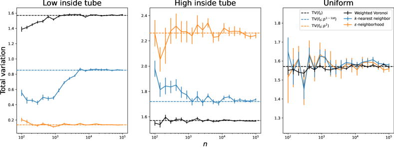
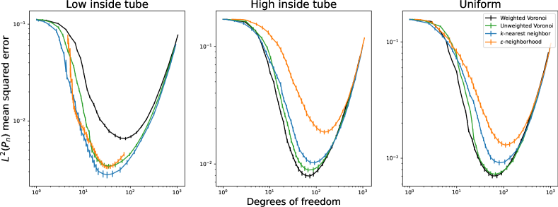
Figure S.1: Results from the TV estimation experiment, with greater connectivity in the kNN and $\varepsilon$-neighborhood graphs. Compare these results to those in Figure 3.

Figure S.2: Results from the function estimation experiment, with greater connectivity in the kNN and $\varepsilon$-neighborhood graphs. Compare these results to those in Figure 5.

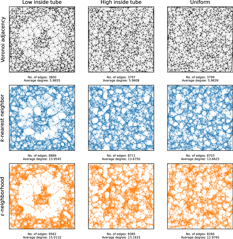
Figure S.3: Visualization of the Voronoi, kNN, and $\varepsilon$-neighborhood graphs, with greater connectivity in the latter two graphs. (The Voronoi graph does not have such an auxiliary tuning parameter.) Compare these graphs to those in Figure 4.

Figure S.4: Extrapolants from graph TV denoising, with greater connectivity in the kNN and $\varepsilon$-neighborhood graphs. Compare these results to those in Figure 6.

Appendix D Proofs for Section 5

D.1 Proof of Theorem 2

From (35), in the discussion preceding Lemma 3, we have

$$\mathbb{E}\|\hat{f}-f_{0}\|_{L^{2}(P)}^{2}\leq\mathbb{E}\Big{[}K_{n}\|\hat{f}-f_{0}\|_{L^{2}(P_{n})}^{2}\Big{]}+2\mathbb{E}\|\bar{f}_{0}-f_{0}\|_{L^{2}(P)}^{2},$$ (S.20)

where

$$K_{n}=2p_{\mathrm{max}}n\cdot\bigg{(}\max_{i=1,\dots,n}\mu(V_{i})\bigg{)}.$$

The second term is bounded by Lemma 3. We now outline the analysis of the first term. As in the $L^{2}(P_{n})$ case we will decompose the error into the case where the design points are well spaced and the case where they are not. This is formalized by the set $\mathscr{X}=\mathscr{X}_{1}\cap\mathscr{X}_{2}$, where $\mathscr{X}_{1},\mathscr{X}_{2}$ are defined in Appendix F. $x_{1:n}$ falls within this set with probability at least $1-3/n^{4}$, and notably on this set,

$$\max_{i}\mu(V_{i})\leq C_{1}\log n/n,$$

for some $C_{1}>0$, since $\mathscr{X}_{2}$ is the set upon which the conclusion of Lemma S.15 holds. We proceed by conditioning,

$$\mathbb{E}\left[K_{n}\lVert\hat{f}-f_{0}\rVert_{L^{2}(P_{n})}^{2}\right] =2p_{\mathrm{max}}\Bigg{(}\mathbb{E}_{x}\left[\mathbb{E}_{z|x}\left[\max_{i}\mu(V_{i})\lVert\hat{\theta}-\theta_{0}\rVert_{2}^{2}\right]{1}\{x_{1:n}\in\mathscr{X}\}\right]$$ (S.21)

$$\hskip 113.81102pt+\mathbb{E}_{x}\left[\mathbb{E}_{z|x}\left[\max_{i}\mu(V_{i})\lVert\hat{\theta}-\theta_{0}\rVert_{2}^{2}\right]{1}\{x_{1:n}\not\in\mathscr{X}\}\right]\Bigg{)}$$

Using the fact that $x_{1:n}\in\mathscr{X}$, the first term on the RHS of (S.21) may be bound,

$$\mathbb{E}_{z|x}\left[\max_{i}\mu(V_{i})\lVert\hat{\theta}-\theta_{0}\rVert_{2}^{2}\right]{1}\{x_{1:n}\in\mathscr{X}\} \leq C_{1}(\log n)\;\mathbb{E}_{z|x}\left[\frac{1}{n}\lVert\hat{\theta}-\theta_{0}\rVert_{2}^{2}\right]\cdot{1}\{x_{1:n}\in\mathscr{X}\}$$

$$\leq C_{2}(\log n)\left(\frac{\lambda\lVert D\theta_{0}\rVert}{n}+\frac{\log^{\alpha}n}{n}\right),$$ (S.22)

where the latter inequality is obtained by following the analysis of Lemma 1. For the second term on the RHS of (S.21), we apply the crude upper bound that $\mu(V_{i})\leq\mu(\Omega)=1$ for all $i=1,\dotsc,n$. Then apply (S.70) to obtain,

$$\mathbb{E}_{z|x}\left[\max_{i}\mu(V_{i})\lVert\hat{\theta}-\theta_{0}\rVert_{2}^{2}\right]{1}\{x_{1:n}\not\in\mathscr{X}\} \leq\mathbb{E}_{z|x}\left[16\lVert z_{1:n}\rVert_{2}^{2}+2\lambda\lVert D\theta_{0}\rVert_{1}\right]{1}\{x_{1:n}\not\in\mathscr{X}\}$$

$$=\left(16n+2\lambda\lVert D\theta_{0}\rVert\right){1}\{x_{1:n}\not\in\mathscr{X}\}.$$

$$\leq\left(16n+4n^{2}\lambda\lVert\theta_{0}\rVert_{\infty}\lVert w\rVert_{\infty}\right){1}\{x_{1:n}\not\in\mathscr{X}\}.$$

$$\leq\left(16n+4n^{2}\lambda\lVert\theta_{0}\rVert_{\infty}\right){1}\{x_{1:n}\not\in\mathscr{X}\},$$ (S.23)

where we also use crude upper bounds on the discrete TV. Substitute (S.22) and (S.23) into (S.21) to obtain,

$$\mathbb{E}\left[K_{n}\lVert\hat{f}-f_{0}\rVert_{L^{2}(P_{n})}^{2}\right] \leq C_{3}\left(\frac{(\log n)\lambda\mathbb{E}\lVert D\theta_{0}\rVert}{n}+\frac{(\log n)^{1+\alpha}}{n}+\lambda n^{2}\mathbb{P}\{x_{1:n}\not\in\mathscr{X}\}\right)$$

$$\leq C_{4}\left(\frac{(\log n)\lambda\mathbb{E}\lVert D\theta_{0}\rVert}{n}+\frac{(\log n)^{1+\alpha}}{n}+\frac{\lambda}{n^{2}}\right)$$

$$\leq C_{5}\left(\frac{\sigma\tau_{n}(\log n)^{3/2+\alpha}\mathbb{E}\lVert D\theta_{0}\rVert}{n}+\frac{(\log n)^{1+\alpha}}{n}\right),$$ (S.24)

where in the final line we have substituted in the value of $\lambda=c\sigma\tau_{n}(\log n)^{1/2+\alpha}$. Apply Lemma 2 to (S.24) and substitute back into (S.20) to obtain the claim. ∎

D.2 Proof of Theorem 3

To establish the lower bound in (30), we follow a classical approach, similar to that outlined in (del Álamo et al., 2021): first we reduce the problem to estimating binary sequences, then we apply Assouad’s lemma (Lemma S.5). This results in a constrained maximization problem, which we analyze to establish the ultimate lower bound.

Step 1: Reduction to estimating binary sequences.

We begin by associating functions $f_{\theta}$ with vertices of the hypercube $\Theta_{S}=\{0,1\}^{S}$, where $S\subseteq[m]^{d}$ for some $m\in\mathbb{N}$. To construct these functions $f_{\theta}$, we partition $\Omega$ into cubes,

$$Q_{i}=\frac{1}{m}(i_{1}-1,i_{1})\times\cdots\times\frac{1}{m}(i_{d}-1,i_{d}),\quad\textrm{for $i\in[m]^{d}$,}$$

and for each $\theta\in\Theta_{S}$ take $f_{\theta}$ to be the piecewise constant function

$$f_{\theta}(x):=a\cdot\sum_{i\in S}\theta_{i}1_{Q_{i}}(x),$$ (S.25)

where $1_{Q_{i}}(x)=1(x\in Q_{i})$ is the characteristic function of $Q_{i}$. Observe that for all $\theta\in\Theta_{S}$, letting $\epsilon:=1/m$,

$$\mathrm{TV}(f_{\theta})\leq 2da|S|\epsilon^{d-1},\quad\textrm{and}\quad\|f_{\theta}\|_{L^{\infty}(\Omega)}\leq a.$$ (S.26)

So long as the constraints in (S.26) are satisfied $\{f_{\theta}:\theta\in\Theta_{S}\}\subseteq\mathrm{BV}_{\infty}(L,M)$, and consequently

$$\inf_{\widehat{f}}\sup_{f_{0}\in\mathrm{BV}_{\infty}(L,M)}\mathbb{E}_{f_{0}}\|\widehat{f}-f_{0}\|_{L^{2}(\Omega)}^{2}\geq\inf_{\widehat{f}}\max_{\theta\in\Theta_{S}}\mathbb{E}_{\theta}\|\widehat{f}-f_{\theta}\|_{L^{2}(\Omega)}^{2}\geq\frac{a^{2}\epsilon^{d}}{4}\inf_{\widehat{\theta}}\max_{\theta\in\Theta}\mathbb{E}_{\theta}\rho(\widehat{\theta},\theta),$$ (S.27)

where $\rho(\theta,\theta^{\prime})=\sum_{i\in S}|\theta_{i}-\theta_{i}^{\prime}|$ is the Hamming distance between vertices $\theta,\theta^{\prime}\in\Theta_{S}$. The second inequality in (S.27) is verified as follows: for a given $\widehat{f}$, letting

$$\widehat{\theta}_{i}=\begin{dcases*}1,\quad\textrm{if $\oint_{Q_{i}}\widehat{f}(x)\,dx\geq a/2$},\\ 0,\quad\textrm{otherwise,}\end{dcases*}$$

it follows that

$$\|\widehat{f}-f_{\theta}\|_{L^{2}(P)}^{2} =\sum_{i\in[m]^{d}}\|\widehat{f}-f_{\theta}\|_{L^{2}(Q_{i})}^{2}$$

$$\geq\sum_{i\in S}\|\widehat{f}-f_{\theta}\|_{L^{2}(Q_{i})}^{2}$$

$$\geq\frac{a^{2}\epsilon^{d}}{4}\sum_{i\in S}1\{\widehat{\theta}_{i}\neq\theta_{i}\}.$$

Step 2: application of Assouad’s lemma.

Given a measurable space $(\mathcal{Z},\mathcal{A})$, and a set of probability measures $\mathcal{M}=\{\mu_{\theta}:\theta\in\Theta\}$ on $(\mathcal{Z},\mathcal{A})$, Assouad’s lemma lower bounds the minimax risk over $\Theta_{S}$, when loss is measured by the Hamming distance $\rho(\widehat{\theta},\theta):=\sum_{i\in S}|\widehat{\theta}_{i}-\theta_{i}|$. We use a form of Assouad’s lemma given in Tsybakov (2009).

Lemma S.5 (Lemma 2.12 of Tsybakov (2009)).

Suppose that for each $\theta,\theta^{\prime}\in\Theta_{S}:\rho(\theta,\theta^{\prime})=1$, we have that $\mathrm{KL}(\mu_{\theta},\mu_{\theta^{\prime}})\leq\alpha<\infty$. It follows that

$$\inf_{\widehat{\theta}}\sup_{\theta\in\Theta_{S}}\mathbb{E}_{\theta}\rho(\widehat{\theta},\theta)\geq\frac{|S|}{2}\max\biggl{(}\frac{1}{2}\exp(-\alpha),(1-\sqrt{\alpha/2})\biggr{)}.$$

To apply Assouad’s lemma in our context, we take $\mathcal{Z}=(\Omega\times\mathbb{R})^{\otimes n}$, and associate each $\theta\in\Theta_{S}$ with the measure $\mu_{\theta}^{(n)}$, the $n$-times product of measure $\mu_{\theta}=\mathrm{Unif}(\Omega)\times N(f_{\theta}(x),1)$. We now lower bound the KL divergence $\mathrm{KL}(\mu_{\theta}^{(n)},\mu_{\theta^{\prime}}^{(n)})$ when $\rho(\theta,\theta^{\prime})=1$; letting $i\in S$ be the single index at which $\theta_{i}\neq\theta_{i}^{\prime}$,

$$\mathrm{KL}(\mu_{\theta},\mu_{\theta^{\prime}}) =\int_{\Omega\times\mathbb{R}}\log\biggl{(}\frac{\phi(y-f_{\theta}(x))}{\phi(y-f_{\theta^{\prime}}(x))}\biggr{)}\phi(y-f_{\theta}(x))\,dy\,dx$$

$$=\int_{Q_{i}\times\mathbb{R}}\log\biggl{(}\frac{\phi(y-a\theta_{i})}{\phi(y-a\theta_{i}^{\prime})}\biggr{)}\phi(y-a\theta_{i})\,dy\,dx$$

$$=\epsilon^{d}\int_{\mathbb{R}}\log\biggl{(}\frac{\phi(y-a\theta_{i}}{\phi(y-a\theta_{i}^{\prime})}\biggr{)}\phi(y-a\theta_{i})\,dy$$

$$=\frac{\epsilon^{d}a^{2}}{2},$$

and it follows that $\mathrm{KL}(\mu_{\theta}^{(n)},\mu_{\theta^{\prime}}^{(n)})\leq n\epsilon^{d}a^{2}/2$. Consequently, so long as (S.26) is satisfied and

$$\frac{n\epsilon^{d}a^{2}}{2}\leq 1,$$

we may apply Lemma S.5, and deduce from (S.27) that

$$\inf_{\widehat{f}}\sup_{f_{0}\in\mathrm{BV}_{\infty}(L,M)}\mathbb{E}_{f_{0}}\|\widehat{f}-f_{0}\|_{L^{2}(\Omega)}^{2}\geq\frac{a^{2}\epsilon^{d}}{4}\inf_{\widehat{\theta}}\max_{\theta\in\Theta}\mathbb{E}_{\theta}\rho(\widehat{\theta},\theta)\geq\frac{a^{2}\epsilon^{d}|S|}{16\exp(1)}.$$ (S.28)

Step 3: Lower bound.

The upshot of Steps 1 and 2 is that the solution to the following constrained maximization problem yields a lower bound on the minimax risk: letting $s=|S|$,

$$\mathrm{maximize}\quad \frac{a^{2}\epsilon^{d}s}{16\exp(1)},$$

$$\mathrm{subject~{}to}\quad 1\leq s\leq\epsilon^{-d},$$

$$as\epsilon^{d-1}\leq\frac{L}{2d},$$

$$a\leq M,$$

$$\frac{na^{2}\epsilon^{d}}{2}\leq 1.$$

Setting $a=M,\epsilon=(\frac{2}{a^{2}n})^{1/d}$, and $s=\frac{L}{2da}\epsilon^{-(d-1)}$ is feasible for this problem if $2dM(\frac{M^{2}n}{2})^{-\frac{(d-1)}{d}}\leq L\leq 2dM(\frac{M^{2}n}{2})^{1/d}$, and implies that the optimal value is at least $\frac{2^{1/d}}{32\exp(1)d}LM(M^{2}n)^{-1/d}$. This implies the claim (30) upon suitable choices of constants. ∎

D.3 Proof of Lemma 1

In this proof, write $\theta_{0}:=(f_{0}(x_{1}),\ldots,f_{0}(x_{n}))$ and $\mathbb{E}_{z|x}[\cdot]=\mathbb{E}[\cdot|x_{1:n}]$. We will use $D$ to represent the modified edge incidence operator with either clipped edge weights or unit weights; the following analysis, which uses the scaling factor $\tau_{n}$, applies to both. Let

$$\mathscr{X}=\mathscr{X}_{1}\cap\mathscr{X}_{2},$$ (S.29)

with $\mathscr{X}_{1},\mathscr{X}_{2}$ as in Section F. By the law of iterated expectation,

$$\mathbb{E}\biggl{[}\frac{1}{n}\|\widehat{\theta}-\theta_{0}\|_{2}^{2}\biggr{]}=\mathbb{E}_{x}\biggl{[}\mathbb{E}_{z|x}\Bigl{[}\frac{1}{n}\|\widehat{\theta}-\theta_{0}\|_{2}^{2}\Bigr{]}\cdot 1\{x_{1:n}\in\mathscr{X}\}\biggr{]}+\mathbb{E}_{x}\biggl{[}\mathbb{E}_{z|x}\Bigl{[}\frac{1}{n}\|\widehat{\theta}-\theta_{0}\|_{2}^{2}\Bigr{]}\cdot 1\{x_{1:n}\not\in\mathscr{X}\}\biggr{]}.$$ (S.30)

We now upper bound each term on the right hand side separately.

For the first term, we will proceed by comparing the penalty operator $D$ to the averaging operator (S.74) and surrogate operator $T$ corresponding to the graph (S.75). By construction $x_{1:n}\in\mathscr{X}$ implies, for $(\xi_{k},u_{k})$ the $k$th singular value/left singular vector of $T$, that

$$\lambda \geq C_{1}\sigma\tau_{n}(\log n)^{1/2+\alpha}$$

$$\geq\max\left\{8\max_{\ell}|\mathcal{C}_{\ell}|^{1/2}\Phi_{1}(D,T,A)\cdot\sigma\sqrt{\log 2n^{4}\cdot\sum_{k=2}^{n}\frac{\|u_{k}\|_{\infty}^{2}}{\xi_{k}^{2}}},\Phi_{2}(D,T,A)\cdot\sigma\sqrt{2\log n}\right\},$$

where the latter inequality follows from combining (S.71), (S.72) with (S.76), (S.77) in the clipped weights case, or (S.78), (S.79) in the unit weights case, for an appropriately chosen $C_{1}$. We may therefore apply Theorem S.1 with $D$, $T$, and $A$, which gives

$$\mathbb{E}_{z|x}\biggl{[}\frac{1}{n}\|\widehat{\theta}-\theta_{0}\|_{2}^{2}\biggr{]}\cdot 1\{x_{1:n}\in\mathscr{X}\}\leq C\biggl{(}\frac{\lambda\|D\theta_{0}\|_{1}}{n}+\frac{\log^{\alpha}n}{n}\biggr{)},$$ (S.31)

On the other hand, to upper bound the second term in (S.30) we use (S.70),

$$\mathbb{E}_{z|x}\Bigl{[}\frac{1}{n}\|\widehat{\theta}-\theta_{0}\|_{2}^{2}\Bigr{]}\cdot 1\{x_{z|x}\not\in\mathscr{X}\} \leq\mathbb{E}_{z|x}\Bigl{[}\frac{16\|z_{1:n}\|_{2}^{2}}{n}+\frac{2\lambda\|D\theta_{0}\|_{1}}{n}\Bigr{]}1\{x_{1:n}\not\in\mathscr{X}\}$$ (S.32)

$$\leq\Bigl{(}16+\frac{2\lambda\|D\theta_{0}\|_{1}}{n}\Bigr{)}1\{x_{1:n}\not\in\mathscr{X}\}.$$

Substituting (S.31) and (S.32) into (S.30), we conclude that

$$\mathbb{E}\biggl{[}\frac{1}{n}\|\widehat{\theta}-\theta_{0}\|_{2}^{2}\biggr{]} \leq C\Bigl{(}\frac{\lambda\mathbb{E}\|D\theta_{0}\|_{1}}{n}+\frac{\log^{\alpha}n}{n}+\mathbb{P}(x_{1:n}\not\in\mathscr{X})\Bigr{)}$$

$$\leq C\Bigl{(}\frac{\lambda\mathbb{E}\|D\theta_{0}\|_{1}}{n}+\frac{\log^{\alpha}n}{n}\Bigr{)}$$

$$=C\Bigl{(}\frac{\sigma\tau_{n}(\log n)^{1/2+\alpha}\mathbb{E}\lVert D\theta_{0}\rVert_{1}}{n}+\frac{\log^{\alpha}n}{n}\Bigr{)},$$ (S.33)

with the second inequality following from Lemma S.13, and the equality from the choice of $\lambda=C_{1}\sigma\tau_{n}(\log n)^{1/2+\alpha}$. ∎

D.4 Proof of Lemma 2

We prove the claim (33) separately for the unit weights and clipped weights case (recall that they differ by a scaling factor $\bar{\tau}_{n}$. We will subsequently abbreviate $f:=f_{0}$ and use the notation $\operatorname{\mathrm{DTV}}(\;\cdot\;;w^{\varepsilon\leftarrow r})$ to denote the $\varepsilon$-neighborhood graph TV, having set $\varepsilon=r$.

D.4.1 Unit weights

Our goal is to upper bound

$$\mathbb{E}\Big{[}\operatorname{\mathrm{DTV}}\Big{(}f(x_{1:n});\,\check{w}^{\mathrm{V}}\Big{)}\Big{]}=n(n-1)\mathbb{E}\Bigl{[}|f(x_{1})-f(x_{2})|1\{\mathcal{H}^{d-1}(\bar{V}_{1}\cap\bar{V}_{2})>0\}\Bigr{]}.$$

By conditioning, we can rewrite the expectation above as

$$p_{\mathrm{max}}^{2}\int_{\Omega}\int_{\Omega}|f(y)-f(x)|\mathbb{P}_{x_{3:n}}\{\mathcal{H}^{d-1}(\bar{V}_{x}\cap\bar{V}_{y})>0\}\,dy\,dx,$$ (S.34)

where $V_{x}=\{z:\|z-x\|_{2}<\|z-x_{i}\|~{}\forall i=2,3,\ldots,n\}$, and likewise for $V_{y}$. Note that $V_{x}$ and $V_{y}$ are random subsets of $\mathbb{R}^{d}$.

We now give an upper bound on the probability that the random cells $\bar{V}_{x}$ and $\bar{V}_{y}$ intersect on a set of positive Hausdorff measure, by relating the problem to uniform concentration of the empirical mass of balls in $\mathbb{R}^{d}$. The upper bound will be crude, in that it may depend on suboptimal multiplicative constants, but sufficient for our purposes. Define $r(V_{x}):=\sup\{\|z-x\|:z\in V_{x}\}$. Observe that if $\|y-x\|>r(V_{x})+r(V_{y})$, then $\bar{V}_{x}\cap\bar{V}_{y}=\emptyset$, since for any $z\in V_{x}$, by the triangle inequality

$$\{\|z-y\|\geq\|y-x\|-\|z-x\|>r(V_{y})\}\Longrightarrow\{z\not\in V_{y}\};$$

therefore

$$\{\mathcal{H}^{d-1}(\bar{V}_{x}\cap\bar{V}_{y})>0\}\Longrightarrow\{\|y-x\|\leq r(V_{x})+r(V_{y})\}.$$

Now, choose $z\in V_{x}$ for which $\|z-x\|=r(V_{x})$. Observe that the ball $B(z,r(V_{x})/2)$ must have empirical mass $0$, i.e., $B(z,r(V_{x})/2)\cap\{x_{3},\ldots,x_{n}\}=\emptyset$ (indeed, this same fact must hold for any $r<r(V_{x})$). Therefore,

$$\mathbb{P}_{x_{3:n}}\{r(V_{x})\geq t\}\leq\mathbb{P}_{x_{3:n}}\Bigl{\{}\exists z:B(z,t/2)\cap\{x_{3},\ldots,x_{n}\}=\emptyset\Bigr{\}}.$$

It follows from Lemma S.14 that if $t_{n,\delta}=c\bigl{(}\frac{1}{n}(d\log n+\log(1/\delta)\bigl{)}^{1/d}<t_{0}$, where $t_{0}$ is a constant not depending on $n,\delta$, then

$$\mathbb{P}_{x_{3:n}}\{\exists z:B(z,t_{n,\delta}/2)\cap\{x_{3},\ldots,x_{n}\}=\emptyset\}\leq\delta.$$

Summarizing this reasoning, we have

$$\mathbb{P}_{x_{3:n}}\{\mathcal{H}^{d-1}(\bar{V}_{x}\cap\bar{V}_{y})>0\} \leq\mathbb{P}_{x_{3:n}}\Bigl{\{}\|y-x\|\leq{r}(V_{x})+{r}(V_{y})\Bigr{\}}$$

$$\leq\mathbb{P}_{x_{3:n}}\Bigl{\{}\|y-x\|\leq 2{r}(V_{x})\Bigr{\}}+\mathbb{P}_{x_{3:n}}\Bigl{\{}\|y-x\|\leq 2{r}(V_{y})\Bigr{\}}$$

$$\leq\mathbb{P}_{x_{3:n}}\Bigl{\{}\exists z:|B(z,\|x-y\|/4)\cap\{x_{3},\ldots,x_{n}\}|=\emptyset\Bigr{\}}$$

$$\qquad\quad+\mathbb{P}_{x_{3:n}}\Bigl{\{}\exists z:|B(z,\|x-y\|/4)\cap\{x_{3},\ldots,x_{n}\}|=\emptyset\Bigr{\}}$$

$$\leq\begin{dcases}2,&\quad\textrm{if $\|x-y\|_{2}\leq 2t_{n,\delta}$},\\ 2\delta,&\quad\textrm{otherwise.}\end{dcases}$$

Setting $\delta_{n}=n^{-(d+1)/d}$ and plugging this back into (S.34), we conclude that if $t_{n,\delta_{n}}<t_{0}$, then

$$\mathbb{E}\Big{[}\operatorname{\mathrm{DTV}}\Big{(}f(x_{1:n});\,\check{w}^{\mathrm{V}}\Big{)}\Big{]} \leq 2n(n-1)\int_{\Omega}\int_{\Omega}|f(y)-f(x)|\Bigl{(}1\{\|x-y\|\leq 2t_{n,\delta_{n}}\}+2\delta_{n}\Bigr{)}\,dy\,dx$$

$$\leq 2\mathbb{E}[\mathrm{DTV}(f;w^{\varepsilon\leftarrow t_{n,\delta}})]+2n^{1-1/d}\int_{\Omega}\int_{\Omega}|f(y)-f(x)|\,dy\,dx.$$ (S.35)

Note that since $\lim_{n\to\infty}t_{n,\delta_{n}}=0$, the condition $t_{n,\delta_{n}}<t_{0}$ will automatically be satisfied for all $n$ sufficiently large.

We now conclude the proof by upper bounding each term in (S.35). The first term refers to the expected $\varepsilon$-neighborhood graph total variation of $f$ when $\varepsilon=t_{n,\delta_{n}}$, and by (S.39) satisfies

$$\mathbb{E}[\mathrm{DTV}_{n,t_{n,\delta}}(f)]\leq Cn^{2}(t_{n,\delta_{n}})^{d+1}\mathrm{TV}(f;\Omega)\leq Cn^{1-1/d}(\log n)^{(d+1)/d}\mathrm{TV}(f;\Omega).$$

The second term above can be upper bounded using a Poincaré inequality for $\mathrm{BV}(\Omega)$ functions, i.e.,

$$\int_{\Omega}\int_{\Omega}|f(y)-f(x)|\,dy\,dx\leq 2\int_{\Omega}|f(x)-\macc@depth\char 1\relax\frozen@everymath{\macc@group}\macc@set@skewchar\macc@nested@a 111{f}(x)|\,dx\leq C\mathrm{TV}(f;\Omega).$$

Plugging these upper bounds back into (S.35) yields the claimed result (33) in the unit weights case. ∎

D.4.2 Clipped weights

We now show (33) using clipped weights. Our goal is to upper bound

$$\mathbb{E}\Big{[}\operatorname{\mathrm{DTV}}\Big{(}f(x_{1:n});\,\tilde{w}^{\mathrm{V}}\Big{)}\Big{]}=n(n-1)\mathbb{E}\Bigl{[}|f(x_{1})-f(x_{2})|\max\{c_{0}n^{-(d-1)/d}{1}\{\mathcal{H}^{d-1}(\bar{V}_{1}\cap\bar{V}_{2})>0\},\mathcal{H}^{d-1}(\bar{V}_{1}\cap\bar{V}_{2})\}\Bigr{]}.$$

By conditioning, we may rewrite the expectation above as

$$p_{\mathrm{max}}^{2}\int_{\Omega}\int_{\Omega}|f(y)-f(x)|\mathbb{E}_{x_{3:n}}\left[\max\{c_{0}n^{-(d-1)/d}{1}\{\mathcal{H}^{d-1}(\bar{V}_{x}\cap\bar{V}_{y})>0\},\mathcal{H}^{d-1}(\bar{V}_{x}\cap\bar{V}_{y})\}\right]\,dy\,dx,$$ (S.36)

where $V_{x}=\{z:\|z-x\|_{2}<\|z-x_{i}\|~{}\forall i=2,3,\ldots,n\}$, and likewise for $V_{y}$. Note that $V_{x}$ and $V_{y}$ are random subsets of $\mathbb{R}^{d}$. We now focus on controlling the inner expectation of (S.36). Upper bound the maximum of two positive functions with their sum to obtain,

$$\mathbb{E}_{3:n}\Big{[}\max\{c_{0}n^{-(d-1)/d} {1}\{\mathcal{H}^{d-1}(\bar{V}_{x}\cap\bar{V}_{y})>0\},\mathcal{H}^{d-1}(\bar{V}_{x}\cap\bar{V}_{y})\}\Big{]}$$ (S.37)

$$\leq c_{0}n^{-(d-1)/d}\mathbb{P}\{\mathcal{H}^{d-1}(\bar{V}_{x}\cap\bar{V}_{y})>0\}+\mathbb{E}\left[\mathcal{H}^{d-1}(\bar{V}_{x}\cap\bar{V}_{y})\right].$$

We recognize the first term on the RHS of (S.37) as having already been analyzed in the unit weights case; we now focus on the second term. The latter “Voronoi kernel” term may be rewritten,

$$\mathbb{E}_{x_{3:n}}\left[\mathcal{H}^{d-1}(\bar{V}_{x}\cap\bar{V}_{y})\right]=\int_{L\cap\Omega}(1-p_{x}(z))^{n-2}dz,$$

where $L=\{z:\lVert x-z\rVert=\lVert y-z\rVert\}$ and $p_{x}(z)=P(B(z,\lVert x-z\rVert))$. Observe by Assumption Assumption A1 that $p_{x}(z)\geq p_{\mathrm{min}}\mu_{d}\lVert x-z\rVert^{d}$, and therefore

$$\int_{L\cap\Omega}(1-p_{x}(z))^{n-2}\leq\exp(-cn\lVert x-z\rVert^{d}),$$

for some $c>0$. Apply Lemma S.19 with $a=2$ to therefore bound,

$$\mathbb{E}_{x_{3:n}}\left[\mathcal{H}^{d-1}(\bar{V}_{x}\cap\bar{V}_{y})\right]\leq C_{1}\left(\frac{{1}\{\lVert x-y\rVert\leq C_{2}(\log n/n)^{1/d}\}}{n^{(d-1)/d}}+\frac{1}{n^{2}}\right),$$ (S.38)

for constants $C_{1},C_{2}>0$. Substitute (S.38) into (S.37) and (S.36) to obtain,

$$\mathbb{E}\Big{[} \operatorname{\mathrm{DTV}}\left(f(x_{1:n});\,\tilde{w}\right)\Big{]}$$

$$\leq p_{\mathrm{max}}^{2}n^{2}\int_{\Omega}\int_{\Omega}|f(y)-f(x)|\Bigg{(}c_{0}n^{-(d-1)/d}\mathbb{P}_{3:n}\{\mathcal{H}(\bar{V}_{x}\cap\bar{V}_{y})>0\}$$

$$\hskip 227.62204pt+C_{1}\frac{{1}\{\lVert x-y\rVert\leq C_{2}(\log n/n)^{1/d}\}}{n^{(d-1)/d}}+\frac{C_{1}}{n^{2}}\Bigg{)}\;dy\;dx$$

$$\leq p_{\mathrm{max}}^{2}c_{0}n^{-(d-1)/d}\mathbb{E}\left[\operatorname{\mathrm{DTV}}(f(x_{1:n});\check{w}^{\mathrm{V}})\right]+p_{\mathrm{max}}^{2}C_{1}n^{-(d-1)/d}\mathbb{E}\left[\operatorname{\mathrm{DTV}}(f(x_{1:n});w^{\varepsilon\leftarrow C_{2}(\log n/n)^{1/d}})\right]$$

$$\hskip 256.0748pt+p_{\mathrm{max}}^{2}C_{1}\int_{\Omega}\int_{\Omega}|f(y)-f(x)|\;dy\;dx$$

$$=T_{1}+T_{2}+T_{3}.$$

We bound each of the terms above in turn. The first term appeals to (33) in the unit weights case, which we have already proved.

$$T_{1} =p_{\mathrm{max}}^{2}c_{0}n^{-(d-1)/d}\mathbb{E}\left[\operatorname{\mathrm{DTV}}(f(x_{1:n});\check{w}^{\mathrm{V}})\right]$$

$$\leq C_{3}n^{-(d-1)/d}n^{(d-1)/d}(\log n)^{1+1/d}\operatorname{\mathrm{TV}}(f)$$

$$=C_{3}(\log n)^{1+1/d}\operatorname{\mathrm{TV}}(f).$$

The second term refers to the expected $\varepsilon$-neighborhood graph total variation of $f$ when $\varepsilon=C_{2}(\log n/n)^{1/d}$, which by (S.39) satisfies,

$$T_{2} =p_{\mathrm{max}}^{2}C_{1}n^{-(d-1)/d}\mathbb{E}\left[\operatorname{\mathrm{DTV}}\Big{(}f(x_{1:n});w^{\varepsilon\leftarrow C_{2}(\log n/n)^{1/d}}\Big{)}\right]$$

$$\leq C_{4}n^{-(d-1)/d}n^{2}(\log n/n)^{(d+1)/d}\operatorname{\mathrm{TV}}(f)$$

$$\leq C_{4}(\log n)^{1+1/d}\operatorname{\mathrm{TV}}(f).$$

The third term can be controlled via the Poincaré inequality,

$$T_{3} =p_{\mathrm{max}}^{2}C_{1}\int_{\Omega}\int_{\Omega}|f(y)-\bar{f}+\bar{f}-f(x)|\;dy\;dx$$

$$\leq C_{5}\int_{\Omega}|f(x)-\bar{f}|\;dx$$

$$\leq C_{5}\operatorname{\mathrm{TV}}(f),$$

where $\bar{f}:=\mathchoice{{\vbox{\hbox{$\textstyle-$ }}\kern-7.83337pt}}{{\vbox{\hbox{$\scriptstyle-$ }}\kern-5.90005pt}}{{\vbox{\hbox{$\scriptscriptstyle-$ }}\kern-4.75003pt}}{{\vbox{\hbox{$\scriptscriptstyle-$ }}\kern-4.25003pt}}\!\int_{\Omega}f$. ∎

D.4.3 $\varepsilon$-neighborhood and kNN expected discrete TV

Lemma S.6.

Under Assumption Assumption A1, there exist constants $c,C_{1},C_{2}>0$ such that for all sufficiently large $n$ and $f_{0}\in\operatorname{\mathrm{BV}}(\Omega)$,

• The $\varepsilon$-neighborhood graph total variation, for any $\varepsilon>0$, satisfies

  $$\mathbb{E}\Big{[}\operatorname{\mathrm{DTV}}\Big{(}f_{0}(x_{1:n};\;w^{\varepsilon})\Big{)}\Big{]}\leq C_{1}n^{2}\varepsilon^{d+1}\operatorname{\mathrm{TV}}(f_{0}).$$ (S.39)

• The $k$-nearest neighbors graph total variation, for any $k\in\mathbb{N}$, satisfies

  $$\mathbb{E}\Big{[}\operatorname{\mathrm{DTV}}\Big{(}f_{0}(x_{1:n};\;w^{k})\Big{)}\Big{]}\leq C_{2}\left(n^{1-1/d}k^{(d+1)/d}+n^{2}\exp(-ck)\right)\operatorname{\mathrm{TV}}(f_{0}).$$ (S.40)

Proof.

$\varepsilon$-neighborhood expected discrete TV.

This follows the proof of Lemma 1 in Green et al. (2021a), with two adaptations to move from Sobolev $H^{2}(\Omega)$ to the $\operatorname{\mathrm{BV}}(\Omega)$: we deal in absolute differences rather than squared differences, and an approximation argument is invoked at the end to account for the existence of non-weakly differentiable functions in $\operatorname{\mathrm{BV}}(\Omega)$.

Begin by rewriting,

$$\mathbb{E}\left[\sum_{i,j=1}^{n}|f(x_{i})-f(x_{j})|\cdot{1}\{\lVert x_{i}-x_{j}\rVert\leq\varepsilon\}\right]=\frac{n(n-1)}{2}\mathbb{E}\left[|f(X^{\prime})-f(X)|K\left(\frac{\lVert X^{\prime}-X\rVert}{\varepsilon}\right)\right],$$ (S.41)

where $X$ and $X^{\prime}$ are random variables independently drawn from $P$ following Assumption Assumption A1 and $K(t)={1}\{t\leq 1\}$. Now, take $\Omega^{\prime}$ to be an arbitrary bounded open set such that $B(x,c_{0})\subseteq\Omega^{\prime}$ for all $x\in\Omega$.

For the remainder of this proof, we assume that (i) $f\in BV(\Omega^{\prime})$ and (ii) $\lVert f\rVert_{BV(\Omega^{\prime})}\leq C^{\prime}\lVert f\rVert_{BV(\Omega)}$ for some constant $C^{\prime}$ independent of $f$. These conditions are guaranteed by the Extension Theorem (Evans, 2010; Section 5.4 Theorem 1), which promises an extension operator $E:W^{1,p}(\Omega)\rightarrow W^{1,p}(\Omega)$ (take $p=1$ and the BV case is established through an approximation argument). We also assume that $f\in C^{\infty}(\Omega)$, which is addressed through via an approximation argument at the end. Since $f\in C^{\infty}(\Omega)$, we may rewrite a difference in terms of an integrated derivative:

$$f(x^{\prime})-f(x)=\int_{0}^{1}\nabla f(x+t(x^{\prime}-x))^{\top}(x^{\prime}-x)dx.$$ (S.42)

It follows that

$$\mathbb{E}\left[|f(X^{\prime})-f(X)|K\left(\frac{\lVert X^{\prime}-X\rVert}{\varepsilon}\right)\leq p_{\text{max}}^{2}\int_{\Omega}\int_{\Omega}|f(x^{\prime})-f(x)|K\left(\frac{\lVert x^{\prime}-x\rVert}{\varepsilon}\right)dx^{\prime}dx\right],$$ (S.43)

and the final step is to bound the double integral. We have

$$\int_{\Omega}\int_{\Omega} |f(x^{\prime})-f(x)|K\left(\frac{\lVert x^{\prime}-x\rVert}{\varepsilon}\right)dx^{\prime}dx$$

$$=\int_{\Omega}\int_{\Omega}\Big{|}\int_{0}^{1}\nabla f(x+t(x^{\prime}-x))^{\top}(x^{\prime}-x)dt\Big{|}K\left(\frac{\lVert x^{\prime}-x\rVert}{\varepsilon}\right)dx^{\prime}dx$$ (FTC)

$$\leq\int_{\Omega}\int_{\Omega}\int_{0}^{1}|\nabla f(x+t(x^{\prime}-x))^{\top}(x^{\prime}-x)|K\left(\frac{\lVert x^{\prime}-x\rVert}{\varepsilon}\right)dtdx^{\prime}dx$$ (Jensen)

$$=\int_{\Omega}\int_{B(0,1)}\int_{0}^{1}|\nabla f(x+t\varepsilon z)^{\top}(\varepsilon z)|K(\lVert z\rVert)\varepsilon^{d}dtdzdx z=(x^{\prime}-x)/\varepsilon$$ ()

$$=\varepsilon^{d+1}\int_{\Omega}\int_{B(0,1)}\int_{0}^{1}|\nabla f(x+t\varepsilon z)^{\top}z|K(\lVert z\rVert)dtdzdx$$

$$\leq\varepsilon^{d+1}\int_{\Omega^{\prime}}\int_{B(0,1)}\int_{0}^{1}|\nabla f(\tilde{x})^{\top}z|K(\lVert z\rVert)dtdzd\tilde{x} \text{($\tilde{x}=x+t\varepsilon z$)}.$$

Next, we apply the Cauchy-Schwarz to $|\nabla f(\tilde{x})^{\top}z|$ to obtain,

$$\int_{B(0,1)}|\nabla f(\tilde{x})^{\top}z|K(\lVert z\rVert)dz \leq\int_{B(0,1)}\lVert\nabla f(\tilde{x})\rVert\lVert z\rVert K(\lVert z\rVert)dz$$

$$=\lVert\nabla f(\tilde{x})\rVert\int_{(B(0,1)}\lVert z\rVert K(\lVert z\rVert)dz$$

$$=C_{d}\lVert\nabla f(\tilde{x})\rVert$$

Substituting back in to the previous derivation, we obtain

$$\int_{\Omega}\int_{\Omega}|f(x^{\prime})-f(x)|K\left(\frac{\lVert x^{\prime}-x\rVert}{\varepsilon}\right)dx^{\prime}dx \leq C_{d}\varepsilon^{d+1}\int_{\Omega^{\prime}}\int_{0}^{1}\lVert\nabla f(\tilde{x})\rVert_{1}dtd\tilde{x}$$

$$=C_{d}\varepsilon^{d+1}\lVert Df\rVert(\Omega^{\prime})$$

$$\leq C_{d}C^{\prime}\varepsilon^{d+1}\lVert Df\rVert(\Omega)$$

Hence,

$$\mathbb{E}\left[\frac{1}{2}\sum_{i,j=1}^{n}|f(x_{i})-f(x_{j})|\cdot{1}\{\lVert x_{i}-x_{j}\rVert\leq\varepsilon\}\right] \leq\frac{n(n-1)}{2}p_{\text{max}}^{2}C_{d}C^{\prime}\varepsilon^{d+1}\lVert Df\rVert(\Omega)$$

$$\leq C_{2}n^{2}\varepsilon^{d+1}\lVert Df\rVert(\Omega)$$

Finally, we provide an approximation argument to justify the assumption that $f\in C^{1}(\Omega^{\prime})$. For a function $f\in\operatorname{\mathrm{BV}}(\Omega^{\prime})$, we may construct a sequence of functions $f_{k}\in C^{\infty}(\Omega^{\prime})$ via mollification such that $f_{k}\rightarrow f$ $\mu$-a.e. (specifically, at all Lebesgue points) and $\lVert Df_{k}\rVert(\Omega^{\prime})\rightarrow\lVert Df\rVert(\Omega^{\prime})$ as $k\rightarrow\infty$ (Evans and Gariepy, 2015; Theorems 4.1 & 5.3). Via an application of Fatou’s lemma, we find that

$$\mathbb{E}\Bigg{[}\frac{1}{2}\sum_{i,j=1}^{n}|f(x_{i})-f(x_{j})| \cdot{1}\{\lVert x_{i}-x_{j}\rVert\leq\varepsilon\}\Bigg{]}$$

$$=\mathbb{E}\left[\frac{1}{2}\sum_{i,j=1}^{n}|\lim_{k\rightarrow\infty}f_{k}(x_{i})-f_{k}(x_{j})|\cdot{1}\{\lVert x_{i}-x_{j}\rVert\leq\varepsilon\}\right]$$

$$=\mathbb{E}\left[\liminf_{k\rightarrow\infty}\frac{1}{2}\sum_{i,j=1}^{n}|f_{k}(x_{i})-f_{k}(x_{j})|\cdot{1}\{\lVert x_{i}-x_{j}\rVert\leq\varepsilon\}\right]$$ (Continuity)

$$\leq\liminf_{k\rightarrow\infty}\mathbb{E}\left[\frac{1}{2}\sum_{i,j=1}^{n}|f_{k}(x_{i})-f_{k}(x_{j})|\cdot{1}\{\lVert x_{i}-x_{j}\rVert\leq\varepsilon\}\right]$$ (Fatou’s lemma)

$$\leq\liminf_{k\rightarrow\infty}Cn^{2}\varepsilon^{d+1}\lVert Df_{k}\rVert(\Omega)$$

$$=Cn^{2}\varepsilon^{d+1}\lVert Df\rVert(\Omega)$$

$k$-nearest neighbors expected discrete TV.

Let $\varepsilon_{k}(x):=\|x-x_{(k)}(x)\|_{2}$ and $\varepsilon_{k}(x,y)=\max\{\varepsilon_{k}(x),\varepsilon_{k}(y)\}$ be data-dependent radii. Notice that

$$\mathrm{DTV}_{n,k}(f)=\frac{1}{2}\sum_{i,j=1}^{n}|f(x_{i})-f(x_{j})|\cdot 1\bigl{\{}\|x_{i}-x_{j}\|\leq\varepsilon_{k}(x_{i},x_{j})\bigr{\}}.$$

By linearity of expectation and conditioning, the expected $k$-nearest neighbor TV can be written as a double integral,

$$\mathbb{E}[\operatorname{\mathrm{DTV}}(f;w^{k})] =n(n-1)\mathbb{E}\Bigl{[}|f(x_{i})-f(x_{j})|~{}1\bigl{\{}\|x_{i}-x_{j}\|\leq\varepsilon_{k}(x_{i},x_{j})\bigr{\}}\Bigr{]}$$

$$=n(n-1)\mathbb{E}\Bigl{[}\mathbb{E}\Bigl{[}|f(x_{i})-f(x_{j})|~{}1\bigl{\{}\|x_{i}-x_{j}\|\leq\varepsilon_{k}(x_{i},x_{j})\bigr{\}}|x_{i},x_{j}\Bigr{]}\Bigr{]}$$

$$\leq n(n-1)\int_{\Omega}\int_{\Omega}|f(y)-f(x)|~{}\mathbb{P}\bigl{\{}\|x-y\|\leq\varepsilon_{k}(x,y)\bigr{\}}\,dx\,dy$$

$$\leq n(n-1)\int_{\Omega}\int_{\Omega}|f(y)-f(x)|~{}\Bigl{(}\mathbb{P}\bigl{\{}\|x-y\|\leq\varepsilon_{k}(x)\bigr{\}}+\mathbb{P}\bigl{\{}\|x-y\|\leq\varepsilon_{k}(x)\bigr{\}}\Bigr{)}\,dx\,dy$$

(The first inequality above is nearly an equality for large $n$, and the second inequality follows by a union bound.)

We now derive an upper bound $\mathbb{P}\bigl{\{}\|x-y\|\leq\varepsilon_{k}(x)\bigr{\}}$. First, observe that the event $\|x-y\|\leq\varepsilon_{k}(x)$ is equivalent to $|B(x,\|y-x\|)\cap x_{1:n}|<k$. Suppose $\|y-x\|\geq C(k/n)^{1/d}$ for $C=(\frac{2d}{p_{\mathrm{min}}\mu_{d}})^{1/d}$. Then

$$p_{k}(x,y):=P(B(x,\|y-x\|))\geq\frac{p_{\mathrm{min}}}{2d}\mu_{d}\|y-x\|^{d}\geq\frac{2k}{n},$$

and applying standard concentration bounds (Bernstein’s inequality) to the tails of a binomial distribution, it follows that

$$\mathbb{P}\biggl{\{}|B(x,\|y-x\|)\cap x_{1:n}|<k\biggr{\}} =\mathbb{P}\biggl{\{}|B(x,\|y-x\|)\cap x_{1:n}|-np_{k}(x,y)<k-np_{k}(x,y)\biggr{\}}$$

$$\leq\exp\biggl{(}-\frac{c(np_{k}(x,y)-k)^{2}}{np_{k}(x,y)+|np_{k}(x,y)-k|}\biggr{)}$$

$$\leq\exp(-ck).$$

Otherwise if $\|y-x\|<C(k/n)^{1/d}$, we use the trivial upper bound $1$ on the probability of an event. To summarize, we have shown

$$\mathbb{P}\bigl{(}\|x-y\|\leq\varepsilon_{k}(x)\bigr{)}\leq\begin{dcases}1,&\quad\textrm{if $\|x-y\|<C(k/n)^{1/d}$,}\\ \exp(-ck),&\quad\textrm{otherwise}.\end{dcases}$$

It follows from (S.40) that

$$\mathbb{E}[\operatorname{\mathrm{DTV}}(f;w^{k})] \leq 2n^{2}\int_{\Omega}\int_{\Omega}|f(y)-f(x)|~{}\Bigl{(}\bigl{(}1\{\|x-y\|<C(k/n)^{1/d}\}\bigr{)}+\exp(-ck)\Bigr{)}\,dx\,dy$$

$$\leq C\bigl{(}\mathbb{E}[\operatorname{\mathrm{DTV}}(f;w^{\varepsilon\leftarrow C(k/n)^{1/d}})]+n^{2}\exp(-ck)\mathrm{TV}(f,\Omega)\bigr{)};$$ (S.44)

the first term on the right hand side of the second inequality is the expected $\varepsilon$-neighborhood graph TV of $f$, with radius $C(k/n)^{1/d}$, while the second term is obtained from the Poincaré inequality

$$\int_{\Omega}\int_{\Omega}|f(y)-f(x)|\,dy\,dx=\int_{\Omega}\int_{\Omega}\biggl{|}f(y)-\bar{f}+\bar{f}-f(x)\biggr{|}\,dy\,dx\leq C\bigl{(}\mathrm{TV}(f;\Omega)\bigr{)},$$ (S.45)

where $\bar{f}=\mathchoice{{\vbox{\hbox{$\textstyle-$ }}\kern-7.83337pt}}{{\vbox{\hbox{$\scriptstyle-$ }}\kern-5.90005pt}}{{\vbox{\hbox{$\scriptscriptstyle-$ }}\kern-4.75003pt}}{{\vbox{\hbox{$\scriptscriptstyle-$ }}\kern-4.25003pt}}\!\int_{\Omega}f(x)\,dx$ is the average of $f$ over $\Omega$. The claimed upper bound (S.40) follows from applying inequality (S.39), with $\varepsilon=C(k/n)^{1/d}$, to (S.44). ∎

D.5 Proof of Lemma 3

Recall that $\lVert g\rVert_{L^{2}(P)}\leq p_{\mathrm{max}}\lVert g\rVert_{L^{2}(\mu)}$ for any $g\in L^{2}(\mu)$ and note that $\|\bar{f_{0}}\|_{L^{\infty}(\mu)}\leq M$ with probability one. By Hölder’s inequality,

$$\mathbb{E}\|\bar{f_{0}}-f_{0}\|_{L^{2}(\mu)}^{2} \leq\mathbb{E}\Bigl{[}\|\bar{f_{0}}-f_{0}\|_{L^{1}(\mu)}\cdot\|\bar{f_{0}}-f_{0}\|_{L^{\infty}(\mu)}\Bigr{]}$$ (S.46)

$$\leq 2M~{}\mathbb{E}\|\bar{f_{0}}-f_{0}\|_{L^{1}(\mu)},$$

and the problem is reduced to upper bounding the expected $L^{1}(\mu)$ loss of $\bar{f_{0}}$. By Fubini’s Theorem we may exchange expectation with integral, giving

$$\mathbb{E}\|\bar{f_{0}}-f_{0}\|_{L^{1}(\mu)} =\int_{\Omega}\mathbb{E}|\bar{f_{0}}(x)-f_{0}(x)|\,dx$$

$$=\int_{\Omega}\int_{\Omega}|f_{0}(y)-f_{0}(x)|p_{x}^{(1)}(y)\,dy\,dx,$$ (S.47)

where $p_{x}^{(1)}(\cdot)$ is the density of $x_{(1)}(x)$. We now give a closed form expression for this density, before proceeding to lower bound (D.5).

Closed-form expression for $p_{x}^{(1)}$.

Suppose $P$ satisfies Assumption Assumption A1. For any $y\in\Omega$ and $0<r<\mathrm{dist}(y,\partial\Omega)$, we have

$$\mathbb{P}\bigl{\{}x_{(1)}(x)\in B(y,r)\bigr{\}} \leq n~{}\mathbb{P}\bigl{\{}x_{1}\in B(y,r)\bigr{\}}\bigl{(}\mathbb{P}\{x_{2}\not\in B(x,\lVert y-x\rVert\}\bigr{)}^{(n-1)}$$

$$\leq np_{\mathrm{max}}\mu\bigl{(}B(y,r)\bigr{)}\Bigl{(}1-P\bigl{(}B(x,\|y-x\|)\bigr{)}\Bigr{)}^{(n-1)}.$$

Taking limits as $r\to 0$ gives

$$p_{x}^{(1)}(y)=\lim_{r\to 0}\frac{\mathbb{P}\bigl{\{}x_{(1)}(x)\in B(y,r)\bigr{\}}}{\mu(B(y,r))}=np_{\mathrm{max}}\Bigl{(}1-P\bigl{(}B(x,\|y-x\|)\bigr{)}\Bigr{)}^{(n-1)}.$$

Upper bound on (D.5).

There exists a constant $C_{d}$ such that for all $x,y\in\Omega$,

$$P\bigl{(}B(x,\|y-x\|)\bigr{)}\geq\frac{p_{\mathrm{min}}}{C_{d}}\mu(B(x,\|y-x\|))=\frac{p_{\mathrm{min}}\mu_{d}}{C_{d}}\|y-x\|^{d}.$$

This implies an upper bound on the density of $x_{(1)}(x)$,

$$p_{x}^{(1)}(y) \leq n\biggl{(}1-\frac{p_{\mathrm{min}}\mu_{d}}{C_{d}}\|y-x\|^{d}\biggr{)}^{(n-1)}$$

$$\leq n\exp\biggl{(}-\frac{p_{\mathrm{min}}\mu_{d}}{C_{d}}\Bigl{(}\frac{\|y-x\|}{n^{-1/d}}\Bigr{)}^{d}\biggr{)},$$

where we have used the inequality $(1-x)^{n}\leq\exp(-nx)$ for $|x|\leq 1$. Using the inequality, valid for all monotone non-increasing functions $g:[0,\infty)\to[0,\infty)$, that $g(t)\leq 1\{t\leq t_{0}\}g(0)+g(t_{0})$, we further conclude that

$$p_{x}^{(1)}(y)\leq n1\{\|y-x\|\leq\varepsilon_{n}^{(1)}\}+\frac{1}{n},$$

for $\varepsilon_{n}^{(1)}:=(\frac{2C_{d}}{p_{\mathrm{min}}\mu_{d}}(\log n/n))^{1/d}$. Plugging back into (D.5), we see that the expected $L^{1}(\mu)$ error is upper bounded by the expected discrete TV of a neighborhood graph with particular kernel and radius, plus a remainder term. Specifically,

$$\mathbb{E}\|\bar{f_{0}}-f_{0}\|_{L^{1}(\mu)} \leq n\int_{\Omega}\int_{\Omega}|f_{0}(y)-f_{0}(x)|1\{\|y-x\|\leq\varepsilon_{n}^{(1)}\}\,dy\,dx+\frac{1}{n}\int_{\Omega}\int_{\Omega}|f_{0}(y)-f_{0}(x)|\,dy\,dx$$

$$\leq n\int_{\Omega}\int_{\Omega}|f_{0}(y)-f_{0}(x)|1\{\|y-x\|\leq\varepsilon_{n}^{(1)}\}\,dy\,dx+\frac{C~{}\mathrm{TV}(f_{0};\Omega)}{n}$$ (S.48)

$$=\frac{1}{n}\mathrm{E}[\operatorname{\mathrm{DTV}}(f_{0};w^{\varepsilon\leftarrow\varepsilon_{n}^{(1)}}))]+\frac{C~{}\operatorname{\mathrm{TV}}(f_{0};\Omega)}{n},$$

where (S.48) above follows from the Poincaré inequality (S.45). We can therefore apply (S.39), which upper bounds the expected $\varepsilon$-neighborhood graph TV, and conclude that

$$\mathbb{E}\|\bar{f_{0}}-f_{0}\|_{L^{1}(\mu)}\leq C\biggl{(}\frac{(\log n)^{1+1/d}}{n^{1/d}}+\frac{1}{n}\biggr{)}\mathrm{TV}(f_{0};\Omega)\leq C\biggl{(}\frac{L(\log n)^{1+1/d}}{n^{1/d}}\biggr{)}.$$

Inserting this upper bound into (S.46) completes the proof of Lemma 3. ∎

D.6 Proof of Theorem 4

The analysis of the $\varepsilon$-neighborhood and kNN TV denoising estimators proceeds identically, so we consider them together. Henceforth let $D$ denote the penalty operator for either estimator and $\hat{f}$ denote their 1NN extrapolants. Follow the proof of Theorem 2 (given in Appendix D.1) to decompose the $L^{2}(P)$ error for some $C>0$,

$$\mathbb{E}\left[\lVert\hat{f}-f_{0}\rVert_{L^{2}(P)}^{2}\right]\leq C\left(\frac{\lambda\log n\;\mathbb{E}\lVert D\theta_{0}\rVert}{n}+\frac{(\log n)^{1+\alpha}}{n}+\frac{LM(\log n)^{1+1/d}}{n^{1/d}}\right),$$ (S.49)

where we have applied Lemma 3 which controls the 1NN extrapolation error. Lemma S.6 provides that under the standard assumptions, there exist constants $C_{1},C_{1}^{\prime}>0$ such that for all sufficiently large $n$ and $\theta_{0}=f_{0}(x_{1:n})$, $f_{0}\in\operatorname{\mathrm{BV}}(\Omega)$,

• setting $\varepsilon=c_{1}(\log^{\alpha}n/n)^{1/d}$,

  $$\mathbb{E}\lVert D^{\varepsilon}\theta_{0}\rVert_{1}\leq C_{1}n^{(d-1)/d}(\log n)^{\alpha+\alpha/d}\operatorname{\mathrm{TV}}(f_{0});$$ (S.50)

• setting $k=c_{1}^{\prime}(\log n)^{3}$,

  $$\mathbb{E}\lVert D^{k}\theta_{0}\rVert_{1}\leq C_{1}^{\prime}n^{(d-1)/d}(\log n)^{3+3/d}\operatorname{\mathrm{TV}}(f_{0}).$$ (S.51)

Take these values of $\varepsilon,k$ and $\lambda=c\sigma(\log n)^{1/2-\alpha}$, $c=c_{2},c_{2}^{\prime}$, and substitute (S.50), (S.51) into (S.49) to obtain the claim. ∎

Note that the $L^{2}(P_{n})$ in-sample error may be obtained similarly, beginning with an analysis identical to that of Lemma 1 to obtain the preliminary upper bound,

$$\mathbb{E}\left[\lVert\hat{f}-f_{0}\rVert_{L^{2}(P_{n})}^{2}\right]\leq C\left(\frac{\lambda\;\mathbb{E}\lVert D\theta_{0}\rVert}{n}+\frac{(\log n)^{1+\alpha}}{n}\right).$$

D.7 Proof of Theorem 5

In this section we prove the upper bound (39). The proof is comprised of several steps and we start by giving a high-level summary.

• We begin in Section D.7.1 by formalizing the estimator $\widehat{f}_{\mathrm{wave}}$ alluded to in Theorem 5, based on hard thresholding of Haar wavelet empirical coefficients.

• Section D.7.2 reviews wavelet coefficient decay of $\mathrm{BV}(\Omega)$ and $L^{\infty}(\Omega)$ functions. These rates of decay imply that the wavelet coefficients of $f_{0}\in\mathrm{BV}_{\infty}(L,M)$ must belong to the normed balls in a pair of Besov bodies, defined formally in (S.58). Besov bodies are sequence-based spaces that reflect the wavelet coefficient decay of functions in Besov spaces.

• Section D.7.3 gives a deterministic upper bound on the squared-$\ell^{2}$ error of thresholding wavelet coefficients when the population-level coefficients belong to intersections of Besov bodies. This deterministic upper bound is based on analyzing two functionals—a modulus of continuity (S.101) and the tail width (S.102)— in the spirit of (Donoho et al., 1995); the difference is that we are considering intersections of Besov bodies.

• The aforementioned modulus of continuity measures the size of the $\ell^{2}$-norm $\|\theta-\theta^{\prime}\|_{2}$ relative to $\ell^{\infty}$-norm $\|\theta-\theta^{\prime}\|_{\infty}$. In Section D.7.4, we give an upper bound on the $\ell^{\infty}$ norm of the difference between sample and population-level wavelet coefficients.

• Finally, in Section D.7.5 we combine the results of Sections D.7.3 and D.7.4 to establish upper bounds on the expected squared-$\ell^{2}$ error of hard thresholding sample wavelet coefficients. The same upper bound will apply to the expected squared-$L^{2}(\Omega)$ error of $\widehat{f}_{\mathrm{wave}}$, by Parseval’s theorem.

D.7.1 Step 1: Hard-thresholding of wavelet coefficients

To define the estimator $\widehat{f}_{\mathrm{wave}}$ that achieves the upper bound in (39), we first review the definition of tensor product Haar wavelets.

Definition 1 (Haar wavelet).

The Haar wavelet $\psi:(0,1)\to\mathbb{R}$ is defined by

$$\psi(x):=1\{x\in(0,1/2]\}-1\{x\in(1/2,1)\}.$$ (S.52)

For each ${\bf i}\in\{0,1\}^{d}\setminus\{(0,\ldots,0)\}$, the tensor product Haar wavelet $\Psi^{\bf i}:(0,1)^{d}\to\mathbb{R}$ is defined by

$$\Psi^{i}(x):=\psi^{i_{1}}(x_{1})\ldots\psi^{i_{d}}(x_{d}),$$ (S.53)

where $\psi^{1}(x)=\psi(x)$ and $\psi^{0}(x)=1$. To ease notation, let $\mathcal{I}=\{0,1\}^{d}\setminus\{(0,\ldots,0)\}$ and $\mathcal{K}(\ell)=[2^{\ell}-1]^{d}$. For each $\ell\in\mathbb{N}\cup\{0\},k\in\mathcal{K}(\ell)$ and ${\bf i}\in\mathcal{I}$, put $\Psi_{\ell k}^{{\bf i}}(x):=2^{\ell d/2}\Psi^{{\bf i}}(2^{\ell}x-k)$. Finally, let $\Phi(x)=1\{x\in(0,1)^{d}\}$. The Haar wavelet basis is the collection $\{\Psi_{\ell k}^{{\bf i}}:\ell\in\mathbb{N},k\in\mathcal{K}(\ell),{\bf i}\in\mathcal{I}\}\cup\{\Phi\}$, and it forms an orthonormal basis of $L^{2}((0,1)^{d})$.

We now describe the estimator $\widehat{f}_{\mathrm{wave}}$, which applies hard thresholding to sample wavelet coefficients. For each $\ell\in\mathbb{N}\cup\{0\},k\in\mathcal{K}(\ell)$ and ${\bf i}\in\mathcal{I}$, write

$$\theta_{\ell k{\bf i}}(f):=\int_{\Omega}\Psi_{\ell k}^{{\bf i}}(x)f(x)\,dx,\quad\widetilde{\theta}_{\ell k{\bf i}}(f):=\frac{1}{n}\sum_{j=1}^{n}f(x_{j})\Psi_{\ell k}^{{\bf i}}(x_{j}),$$

for the population-level and empirical wavelet coefficients of a given $f\in L^{2}(\Omega)$. The sample wavelet coefficient is $\widetilde{\theta}_{\ell k{\bf i}}(y_{1:n})$. The hard thresholding estimator we use is defined with respect to a threshold $\lambda>0$ and a truncation level $\ell^{\ast}\in\mathbb{N}\cup\{0\}$ as

$$\widehat{\theta}_{\ell k{\bf i}}^{(\lambda,\ell^{\ast})}:=\begin{dcases}\widetilde{\theta}_{\ell k{\bf i}}(y_{1:n})\cdot 1\{\widetilde{\theta}_{\ell k{\bf i}}(y_{1:n})\geq\lambda\},&\textrm{$\ell=0,\ldots,\ell^{\ast}$}\\ 0,&\textrm{$\ell\geq\log_{2}(n)/d+1,$}\end{dcases}$$ (S.54)

and we map the sequence estimate $\widehat{\theta}^{(\lambda,\ell^{\ast})}=\bigl{(}\widehat{\theta}_{\ell k{\bf i}}^{(\lambda,\ell^{\ast})}:\ell\in\mathbb{N},k\in\mathcal{K}(\ell),{\bf i}\in\mathcal{I}\bigr{)}$ to the function

$$\widehat{f}^{(\lambda,\ell^{\ast})}(x)=\macc@depth\char 1\relax\frozen@everymath{\macc@group}\macc@set@skewchar\macc@nested@a 111{y}+\sum_{\ell\in\mathbb{N}}\sum_{k\in\mathcal{K}(\ell),{\bf i}\in\mathcal{I}}\widehat{\theta}_{\ell k{\bf i}}^{(\lambda,\ell^{\ast})}\Psi_{\ell k}^{{\bf i}}(x),$$ (S.55)

where $\macc@depth\char 1\relax\frozen@everymath{\macc@group}\macc@set@skewchar\macc@nested@a 111{y}=\frac{1}{n}\sum_{i=1}^{n}y_{i}$ is the sample average of the responses. (S.55) defines a family of estimators depending on the threshold $\lambda$, and the estimator $\widehat{f}_{\mathrm{wave}}$ is the hard thresholding estimate $\widehat{f}^{(\lambda,\ell^{\ast})}$ with the specific choices $\lambda=8n^{-1/2}\log^{3/2}(2n/\delta)$ and $\ell^{\ast}=\log_{2}(n)/d$.

D.7.2 Step 2: Wavelet decay

In this section we recall the wavelet coefficient decay of functions in $\mathrm{BV}(\Omega)$ and in $L^{\infty}(\Omega)$. For each $\ell\in\mathbb{N}\cup\{0\}$, define

$$\theta_{\ell\cdot}(f)=\bigl{(}\theta_{\ell k}^{{{\bf i}}}(f):k\in\mathcal{K}(\ell),{\bf i}\in\mathcal{I}\bigr{)}.$$

and write $\theta(f)$ for the vector with entries $\theta(f)_{\ell}:=\theta_{\ell\cdot}(f)$.

Lemma S.7.

Let $f\in L^{\infty}(\Omega)$. Then for all $\ell\in\mathbb{N}\cup\{0\}$,

$$\|\theta_{\ell\cdot}(f)\|_{\infty}\leq 2^{-\ell d/2}\|f\|_{L^{\infty}(\Omega)}.$$ (S.56)

Lemma S.8.

There exists a constant $C_{1}$ such that for all $f\in\mathrm{BV}(\Omega)$ and $\ell\in\mathbb{N}\cup\{0\}$,

$$\|\theta_{\ell\cdot}(f)\|_{1}\leq C_{1}2^{-\ell(1-d/2)}\mathrm{TV}(f;\Omega).$$ (S.57)

The decay rates established by Lemmas S.7 and S.8 imply that if $f_{0}\in\mathrm{BV}_{\infty}(L,M)$, then $\theta(f_{0})$ belongs to $\Theta_{\infty}^{0,\infty}(M)$ and $\Theta_{\infty}^{1,1}(L)$, where $\Theta_{\infty}^{s,p}(C)$ consists of sequences $\theta$ for which

$$\|\theta\|_{\Theta_{\infty}^{s,p}}:=\sup_{\ell\in\mathbb{N}\cup\{0\}}2^{\ell(s+d/2-d/p)}\|\theta_{\ell\cdot}\|_{p}<C.$$ (S.58)

The sets $\Theta_{\infty}^{s,p}(C)$ can be interpreted as normed balls in Besov bodies, since a function $f$ belongs to the Besov space $B_{\infty}^{s,p}$ if and only if its coefficients in a suitable wavelet basis satisfy $\|\theta(f)\|_{\Theta_{\infty}^{s,p}}<\infty$.

The conclusions of Lemmas S.7 and S.8 are generally well-understood (see for instance Giné and Nickl (2021) for the upper bound on wavelet decay of $L^{\infty}(\Omega)$ functions when $d=1$, and Cohen et al. (2003) for the wavelet decay of $\mathrm{BV}(\Omega)$ functions). For purposes of completeness only, we include proofs of these results in Appendix G.3.1.

D.7.3 Step 3: Deterministic upper bound on $\ell^{2}$-error

In this section, we analyze the $\ell^{2}$-error of the hard-thresholding estimator $\widehat{\theta}^{(\lambda,\ell^{\ast})}$. Specifically, we upper bound the magnitude of $\|\widehat{\theta}^{(\lambda,\ell^{\ast})}-\theta(f_{0})\|_{2}$ as a function of the $\ell^{\infty}$ distance between the (truncated) sample and population-level wavelet coefficients, i.e the quantity

$$\epsilon_{n}:=\|(\widetilde{\theta}(y_{1:n})-\theta(f_{0}))_{\leq\ell^{\ast}}\|_{\infty},$$

where

$$(\theta_{\leq\ell^{\ast}})_{\ell k}^{{\bf i}}:=\begin{dcases*}\theta_{\ell k}^{{\bf i}},&\quad{if $\ell\leq\ell^{\ast}$,}\\ 0,&\quad{otherwise.}\end{dcases*}$$

Note that this upper bound is purely deterministic.

Proposition S.2.

Suppose $\theta(f_{0})\in\Theta_{\infty}^{0,\infty}(M)\cap\Theta_{\infty}^{1,1}(L)$. Then there exists a constant $C_{3}$ that does not depend on $n,M$ or $L$ for which the following statement holds: if $\lambda\geq 2\epsilon_{n}$, then the estimator $\widehat{\theta}^{(\lambda,\ell^{\ast})}$ of (S.55) satisfies the upper bound

$$\|\widehat{\theta}^{(\lambda,\ell^{\ast})}-\theta(f_{0})\|_{2}^{2}\leq 4C_{1}LM2^{-\ell^{\ast}}+C_{3}\cdot\begin{dcases*}L\lambda\max\{1,1/M,\log_{2}(M/\lambda)\},&\quad{if $d=2$}\\ L^{2/d}\lambda^{4/(2+d)}+LM\Bigl{(}\frac{\lambda}{M}\Bigr{)}^{2/d},&\quad{if $d\geq 3$.}\end{dcases*}$$ (S.59)

The proof is deferred to Appendix G.3.2.

D.7.4 Step 4: Uniform convergence of wavelet coefficients

Lemma S.9 gives an upper bound on the maximum difference between sample and population-level wavelet coefficients that holds uniformly over all $\ell=0,\ldots,\log_{2}(n)/d$, $k\in\mathcal{K}(\ell)$ and ${\bf i}\in\mathcal{I}$. Its proof is deferred to Appendix G.3.3.

Lemma S.9.

Suppose we observe data $(x_{1},y_{1}),\ldots,(x_{n},y_{n})$ according to (1), where $f_{0}\in L^{\infty}(\Omega;M)$. There exists a constant $C_{4}$ not depending on $n$ such that the following statement holds for all $\delta>0$: with probability at least $1-C_{4}\delta$,

$$\|(\widetilde{\theta}(y_{1:n})-\theta(f_{0}))_{\leq\log_{2}(n)/d}\|_{\infty}\leq\underbrace{\frac{4\log^{3/2}(2n/\delta)}{\sqrt{n}}+\frac{\sqrt{12}M\sqrt{\log(2n/\delta)}}{\sqrt{n}}}_{:=\delta_{n}}.$$ (S.60)

D.7.5 Step 5: Upper bound on risk

We are now ready to prove the stated upper bound (39). In this section we take $\lambda=2\delta_{n}$ and $\ell^{\ast}=\log_{2}(n)/d$. Combining Proposition S.2 and Lemma S.9, we have that with probability at least $1-C_{4}\delta$,

$$\|\widehat{\theta}^{(\lambda,\ell^{\ast})}-\theta_{0}(f)\|_{2}^{2}\leq\frac{4C_{1}LM}{n^{1/d}}+C_{3}\cdot\begin{dcases*}2L\delta_{n}\max\{1,1/M,\log_{2}(M/2\delta_{n})\},&\quad{if $d=2$,}\\ L^{2/d}(2\delta_{n})^{4/(2+d)}+LM\Bigl{(}\frac{2\delta_{n}}{M}\Bigr{)}^{2/d},&\quad{if $d\geq 3$.}\end{dcases*}$$ (S.61)

The following lemma allows us to convert this upper bound, which holds with probability $1-C_{4}\delta$, to an upper bound which holds in expectation. Its proof is deferred to Appendix G.3.4.

Lemma S.10.

Let $X>0$ be a positive random variable. Suppose there exist positive numbers $A_{1},\ldots,A_{K}$, $a_{1},\ldots,a_{K}$, $b_{1},\ldots,b_{K}>1$ and $B$ such that for all $\delta\in(0,1)$,

$$\mathbb{P}\Bigl{(}X>\sum_{k=1}^{K}A_{k}\log^{a_{k}}(b_{k}/\delta)\Bigr{)}\leq B\delta.$$

Then there exists a constant $C_{5}$ depending only on $a_{1},\ldots,a_{k}$ and $B$ such that

$$\mathbb{E}[X]\leq C_{5}\sum_{k=1}^{K}A_{k}(\log b_{k})^{a_{k}}.$$

Now we use Lemma S.10 to complete the proof of Theorem 5. Note that for any $a>0$,

$$\delta_{n}^{a}\leq\frac{2^{a}}{\sqrt{n}}\Bigl{(}(\log(2n/\delta))^{3a/2}+M\sqrt{\log(2n/\delta)}\Bigr{)}.$$

Thus we may can apply Lemma S.10 to (S.61), which, setting $\delta_{n}^{\ast}=\frac{4}{\sqrt{n}}\Bigl{(}(\log 2n)^{3/2}+M\log(n)^{1/2}\Bigr{)}$, gives

$$\mathbb{E}\|\widehat{\theta}^{(\lambda,\ell^{\ast})}-\theta_{0}(f)\|_{2}^{2}\leq\frac{4C_{1}LM}{n^{1/d}}+C_{6}\cdot\begin{dcases*}2L\delta_{n}^{\ast}\max\{1,1/M,\log_{2}(M\sqrt{n})\},&\quad{if $d=2$,}\\ L^{2/d}(2\delta_{n}^{\ast})^{4/(2+d)}+LM\Bigl{(}\frac{2\delta_{n}^{\ast}}{M}\Bigr{)}^{2/d},&\quad{if $d\geq 3$.}\end{dcases*}$$ (S.62)

where $C_{6}=2C_{3}C_{5}$.

Finally, we translate this to an upper bound on the expected risk of $\widehat{f}_{\mathrm{wave}}=\widehat{f}^{(\lambda,\ell^{\ast})}$. Since $\{\Psi_{\ell k}^{{\bf i}},\ell\in\mathbb{N}\cup\{0\},k\in\mathcal{K}(\ell),{\bf i}\in\mathcal{I}\}\cup\{\Phi\}$ forms an orthonormal basis of $L^{2}(\Omega)$, by Parseval’s theorem we have

$$\|\widehat{f}^{(\lambda,\ell^{\ast})}-f_{0}\|_{L^{2}(\Omega)}^{2}=(\macc@depth\char 1\relax\frozen@everymath{\macc@group}\macc@set@skewchar\macc@nested@a 111{y}-\mathbb{E}[f_{0}])^{2}+\|\widehat{\theta}^{(\lambda,\ell^{\ast})}-\theta(f_{0})\|_{2}^{2}.$$

Taking expectation on both sides, the claimed upper bound (39) follows by (S.62), upon proper choice of constant $C=\max\{4C_{1},16C_{6}\}$. ∎

Appendix E Analysis of graph TV denoising

In this section, we review tools for analyzing graph total variation denoising. Suppose an unknown $\theta_{0}\in\mathbb{R}^{n}$ and observations $y_{1},\dotsc,y_{n}$,

$$y_{i}=\theta_{0i}+z_{i},\qquad i=1,\dotsc,n,$$ (S.63)

where $z_{i}\sim\mathcal{N}(0,\sigma^{2})$. The graph total variation denoising estimator $\hat{\theta}$ associated with a graph $G=(V,E)$, $|V|=n$, is given by

$$\hat{\theta}=\mathop{\mathrm{argmin}}_{\theta\in\mathbb{R}^{n}}\frac{1}{2}\lVert y_{1:n}-\theta\rVert_{2}^{2}+\lambda\lVert D\theta\rVert_{1},$$ (S.64)

where $D\in\mathbb{R}^{m\times n}$ is the edge incidence matrix of $G$.

The initial analysis of graph total variation denoising was performed by Hutter and Rigollet (2016) for the two-dimensional grid. Sadhanala et al. (2016) subsequently generalized the analysis to $d$-dimensional lattices, and Wang et al. (2016) provided tools for the analysis of general graphs. These techniques rely on direct analysis of properties of graph $G$ and the penalty $D$ in induces, which is tractable when $G$ has a known and regular properties (e.g., it is a lattice graph).

Unfortunately, direct analysis on $D$ may not always be feasible. It may be possible, however, to compare the operator $D$ to a surrogate operator whose properties we analyze instead. For our purposes, we compare $D$ to a linear operator which first takes averages on a partition, and then computes differences across cells of the partition. Comparison to this type of surrogate operator was used by Padilla et al. (2020) to bound the risk of graph total variation denoising in probability; the following theorem provides an analogous risk bound in expectation. We note that elements of the “surrogate operator analysis” are also found in Padilla et al. (2018).

Theorem S.1.

Suppose we observe data according to model (S.63) and compute the graph TV denoising estimator $\hat{\theta}$ of (S.64). Let $A\in\mathbb{R}^{n\times n}$ denote an averaging operator over $\bar{N}$ groups of the form,

$$A=\begin{bmatrix}n_{1}^{-1}\mathbf{1}_{n_{1}}\mathbf{1}_{n_{1}}^{\top}&0&\ldots&0\\ 0&n_{2}^{-1}\mathbf{1}_{n_{2}}\mathbf{1}_{n_{2}}^{\top}&\ldots&0\\ \vdots&\vdots&\ddots&\vdots\\ 0&0&\ldots&n_{\bar{N}}^{-1}\mathbf{1}_{n_{\bar{N}}}\mathbf{1}_{n_{\bar{N}}}^{\top}\end{bmatrix},$$

with $M:=\max_{j}n_{j}$, and let $\bar{A}\in\mathbb{R}^{\bar{N}\times n}$ be the same matrix with redundant rows removed. Further let $T\in\mathbb{R}^{\bar{m}\times\bar{N}}$ be a surrogate penalty operator, with singular value decomposition $T=U\Sigma V^{\top}$, such that

$$\lVert T\bar{A}\theta\rVert_{1} \leq\Phi_{1}(D,T,A)\lVert D\theta\rVert_{1},$$ (S.65)

$$\lVert(I-A)\theta\rVert_{1} \leq\Phi_{2}(D,T,A)\lVert D\theta\rVert_{1},$$ (S.66)

for quantities $\Phi_{1}(D,T,A),\Phi_{2}(D,T,A)$ that may depend on $n$, for all $\theta\in\mathbb{R}^{n}$. If the penalty parameter

$$\lambda>\max\left\{8M^{1/2}\Phi_{1}(D,T,A)\cdot\sigma\sqrt{\log(2n^{4})\sum_{k=2}^{\bar{N}}\frac{\lVert u_{k}\rVert_{\infty}^{2}}{\xi_{k}^{2}}},\Phi_{2}(D,T,A)\cdot\sigma\sqrt{2\log(n)}\right\}$$ (S.67)

where $u_{k}$ is the $k$th column of $U$ and $\xi_{k}$ the $k$th diagonal entry of $\Sigma$, then there exists a constant $C>0$ such that

$$\mathbb{E}\left[\frac{1}{n}\lVert\hat{\theta}-\theta_{0}\rVert_{2}^{2}\right]\leq C\left(\frac{\lambda\lVert D\theta_{0}\rVert_{1}}{n}+\frac{M\mathrm{nullity}(T)}{n}\right).$$ (S.68)

Proof.

We follow the approach of Padilla et al. (2020), with adaptations to provide a bound in expectation rather than in probability. From the basic inequality,

$$\lVert\hat{\theta}-\theta_{0}\rVert_{2}^{2}\leq 2\langle{z_{1:n}},\hat{\theta}-\theta_{0}\rangle+\lambda(\lVert D\theta_{0}\rVert_{1}-\lVert D\hat{\theta}\rVert_{1}),$$

where ${z_{1:n}}\in\mathbb{R}^{n}$ is the vector of error terms $z_{i}$, $i=1,\dotsc,n$. We provide two deterministic bounds under the “good case” that the error term falls into the set,

$$\mathcal{Z}_{\lambda}=\left\{{z_{1:n}}:\max\left\{M^{1/2}\Phi_{1}(D,T,A)\sup_{\bar{A}\theta\in\mathrm{row}(T):\lVert T\bar{A}\theta\rVert_{1}\leq 1}|\langle\macc@depth\char 1\relax\frozen@everymath{\macc@group}\macc@set@skewchar\macc@nested@a 111{{z_{1:n}}},\bar{A}\theta\rangle|,\Phi_{2}(D,T,A)\lVert{z_{1:n}}\rVert_{\infty}\right\}\leq\frac{\lambda}{8}\right\},$$ (S.69)

where $\macc@depth\char 1\relax\frozen@everymath{\macc@group}\macc@set@skewchar\macc@nested@a 111{{z_{1:n}}}\in\mathbb{R}^{\bar{N}}$ has entries $\macc@depth\char 1\relax\frozen@everymath{\macc@group}\macc@set@skewchar\macc@nested@a 111{{z_{1:n}}}_{j}=n_{j}^{1/2}(\bar{A}{z_{1:n}})_{j}$, and under the “bad case” that ${z_{1:n}}\not\in\mathcal{Z}_{\lambda}$.

Upper bound in the “good case”.

Decompose the first term on the RHS,

$$\langle{z_{1:n}},\hat{\theta}-\theta_{0}\rangle =\langle{z_{1:n}},\hat{\theta}-A\hat{\theta}\rangle+\langle{z_{1:n}},A\theta_{0}-\theta_{0}\rangle+\langle{z_{1:n}},A(\theta_{0}-\hat{\theta})\rangle$$

$$\leq\langle{z_{1:n}},A(\theta_{0}-\hat{\theta})\rangle+\lVert{z_{1:n}}\rVert_{\infty}(\lVert(I-A)\hat{\theta}\rVert_{1}+\lVert(I-A)\theta_{0}\rVert_{1})$$

$$\leq\langle{z_{1:n}},A(\theta_{0}-\hat{\theta})\rangle+\lVert{z_{1:n}}\rVert_{\infty}\Phi(D,T,A)(\lVert D\theta_{0}\rVert_{1}+\lVert D\hat{\theta}\rVert_{1}),$$

where the final inequality follows from (S.66). Observe that we may rewrite, for any $\theta\in\mathbb{R}^{n}$,

$$\langle{z_{1:n}},A\theta\rangle =\sum_{j=1}^{\bar{N}}\sum_{i=1}^{n_{j}}{z_{1:n}}_{(\sum_{k=1}^{j-1}n_{k})+i}(\bar{A}\theta)_{j}$$

$$\stackrel{{\scriptstyle d}}{{=}}\sum_{j=1}^{\bar{N}}n_{j}^{1/2}{z_{1:n}}_{j}(\bar{A}\theta)_{j}$$

$$\Rightarrow\langle{z_{1:n}},A\theta\rangle \leq M^{1/2}|\langle\macc@depth\char 1\relax\frozen@everymath{\macc@group}\macc@set@skewchar\macc@nested@a 111{{z_{1:n}}},\bar{A}\theta\rangle|$$

$$\leq M^{1/2}\left|\langle\operatorname{\mathrm{proj}}_{V}(\macc@depth\char 1\relax\frozen@everymath{\macc@group}\macc@set@skewchar\macc@nested@a 111{{z_{1:n}}}),\bar{A}\theta\rangle+\langle\operatorname{\mathrm{proj}}_{V^{\perp}}(\macc@depth\char 1\relax\frozen@everymath{\macc@group}\macc@set@skewchar\macc@nested@a 111{{z_{1:n}}}),\bar{A}\theta\rangle\right|$$

$$\leq M^{1/2}\left|\lVert\operatorname{\mathrm{proj}}_{V}(\macc@depth\char 1\relax\frozen@everymath{\macc@group}\macc@set@skewchar\macc@nested@a 111{{z_{1:n}}})\rVert_{2}\lVert\bar{A}\theta\rVert_{2}+\langle\operatorname{\mathrm{proj}}_{V^{\perp}}(\macc@depth\char 1\relax\frozen@everymath{\macc@group}\macc@set@skewchar\macc@nested@a 111{{z_{1:n}}}),\bar{A}\theta\rangle\right|$$

$$\leq M^{1/2}\left(\lVert\operatorname{\mathrm{proj}}_{V}(\macc@depth\char 1\relax\frozen@everymath{\macc@group}\macc@set@skewchar\macc@nested@a 111{{z_{1:n}}})\rVert_{2}\lVert\theta\rVert_{2}+|\langle\operatorname{\mathrm{proj}}_{V^{\perp}}(\macc@depth\char 1\relax\frozen@everymath{\macc@group}\macc@set@skewchar\macc@nested@a 111{{z_{1:n}}}),\bar{A}\theta\rangle|\right|,$$

where $\macc@depth\char 1\relax\frozen@everymath{\macc@group}\macc@set@skewchar\macc@nested@a 111{{z_{1:n}}}\in\mathbb{R}^{\bar{N}}$ has independent $\mathcal{N}(0,\sigma^{2})$ entries and $V=\mathrm{null}(T)$. Substitute back in to obtain,

$$\lVert\hat{\theta}-\theta_{0}\rVert_{2}^{2} \leq 2M^{1/2}(\lVert\operatorname{\mathrm{proj}}_{V}(\macc@depth\char 1\relax\frozen@everymath{\macc@group}\macc@set@skewchar\macc@nested@a 111{{z_{1:n}}})\rVert_{2}\lVert\hat{\theta}-\theta_{0}\rVert_{2}+|\langle\operatorname{\mathrm{proj}}_{V^{\perp}}(\macc@depth\char 1\relax\frozen@everymath{\macc@group}\macc@set@skewchar\macc@nested@a 111{{z_{1:n}}}),\bar{A}(\hat{\theta}-\theta_{0})\rangle|)$$

$$\qquad\qquad+2\lVert{z_{1:n}}\rVert_{\infty}\Phi(D,T,A)(\lVert D\theta_{0}\rVert_{1}+\lVert D\hat{\theta}\rVert_{1})+\lambda(\lVert D\theta_{0}\rVert_{1}-\lVert D\hat{\theta}\rVert_{1}),$$

and consequently,

$$\lVert\hat{\theta}-\theta_{0}\rVert_{2}( \lVert\hat{\theta}-\theta_{0}\rVert_{2}-2M^{1/2}\lVert\operatorname{\mathrm{proj}}_{V}(\macc@depth\char 1\relax\frozen@everymath{\macc@group}\macc@set@skewchar\macc@nested@a 111{{z_{1:n}}})\rVert_{2})$$

$$\leq 2M^{1/2}|\langle\operatorname{\mathrm{proj}}_{V^{\perp}}(\macc@depth\char 1\relax\frozen@everymath{\macc@group}\macc@set@skewchar\macc@nested@a 111{{z_{1:n}}}),\bar{A}(\hat{\theta}-\theta_{0})\rangle|+2\lVert{z_{1:n}}\rVert_{\infty}\Phi(D,T,A)(\lVert D\theta_{0}\rVert_{1}+\lVert D\hat{\theta}\rVert_{1})+\lambda(\lVert D\theta_{0}\rVert_{1}-\lVert D\hat{\theta}\rVert_{1})$$

Case 1. $\lVert\hat{\theta}-\theta_{0}\rVert_{2}\leq 4M^{1/2}\lVert\operatorname{\mathrm{proj}}_{V}(\macc@depth\char 1\relax\frozen@everymath{\macc@group}\macc@set@skewchar\macc@nested@a 111{{z_{1:n}}})\rVert_{2}$.
Case 2. $\lVert\hat{\theta}-\theta_{0}\rVert_{2}>4M^{1/2}\lVert\operatorname{\mathrm{proj}}_{V}(\macc@depth\char 1\relax\frozen@everymath{\macc@group}\macc@set@skewchar\macc@nested@a 111{{z_{1:n}}})\rVert_{2}$. Then,

$$\lVert\hat{\theta}-\theta_{0}\rVert_{2}^{2} \leq 4M^{1/2}|\langle\operatorname{\mathrm{proj}}_{V^{\perp}}(\macc@depth\char 1\relax\frozen@everymath{\macc@group}\macc@set@skewchar\macc@nested@a 111{{z_{1:n}}}),\bar{A}(\hat{\theta}-\theta_{0})\rangle|+4\lVert{z_{1:n}}\rVert_{\infty}\Phi(D,T,A)(\lVert D\theta_{0}\rVert_{1}+\lVert D\hat{\theta}\rVert_{1})+\lambda(\lVert D\theta_{0}\rVert_{1}-\lVert D\hat{\theta}\rVert_{1}).$$

We then bound,

$$|\langle\operatorname{\mathrm{proj}}_{V^{\perp}}(\macc@depth\char 1\relax\frozen@everymath{\macc@group}\macc@set@skewchar\macc@nested@a 111{{z_{1:n}}}),\bar{A}(\hat{\theta}-\theta_{0})\rangle| =\left|\left\langle\operatorname{\mathrm{proj}}_{V^{\perp}}(\macc@depth\char 1\relax\frozen@everymath{\macc@group}\macc@set@skewchar\macc@nested@a 111{{z_{1:n}}}),\frac{\bar{A}(\hat{\theta}-\theta_{0})}{\lVert T\bar{A}(\hat{\theta}-\theta_{0})\rVert_{1}}\right\rangle\lVert T\bar{A}(\hat{\theta}-\theta_{0})\rVert_{1}\right|$$

$$\leq\sup_{\bar{A}\theta\in V^{\perp}:\lVert T\bar{A}\theta\rVert_{1}\leq 1}|\langle\macc@depth\char 1\relax\frozen@everymath{\macc@group}\macc@set@skewchar\macc@nested@a 111{{z_{1:n}}},\bar{A}\theta\rangle|\lVert T\bar{A}(\hat{\theta}-\theta_{0})\rVert_{1}$$

$$\leq\sup_{\bar{A}\theta\in V^{\perp}:\lVert T\bar{A}\theta\rVert_{1}\leq 1}|\langle\macc@depth\char 1\relax\frozen@everymath{\macc@group}\macc@set@skewchar\macc@nested@a 111{{z_{1:n}}},\bar{A}\theta\rangle|\Phi(D,T,A)(\lVert D\hat{\theta}\rVert_{1}+\lVert D\theta_{0}\rVert_{1}),$$

where the last inequality follows by (S.66). Conditioning on ${z_{1:n}}\in\mathcal{Z}_{\lambda}$, we find that under Case 2,

$$\lVert\hat{\theta}-\theta_{0}\rVert_{2}^{2} \leq\frac{\lambda}{2}(\lVert D\hat{\theta}\rVert_{1}+\lVert D\theta_{0}\rVert_{1})+\frac{\lambda}{2}(\lVert D\hat{\theta}\rVert_{1}+\lVert D\theta_{0}\rVert_{1})+\lambda(\lVert D\theta_{0}\rVert_{1}-\lVert D\hat{\theta}\rVert_{1})$$

$$\leq 2\lambda\lVert D\theta_{0}\rVert_{1}.$$

Therefore, conditioning on ${z_{1:n}}\in\mathcal{Z}_{\lambda}$ and combining Case 1 and Case 2, we obtain that

$$\lVert\hat{\theta}-\theta_{0}\rVert_{2}^{2} \leq 16M\lVert\operatorname{\mathrm{proj}}_{V}(\macc@depth\char 1\relax\frozen@everymath{\macc@group}\macc@set@skewchar\macc@nested@a 111{{z_{1:n}}})\rVert_{2}^{2}+2\lambda\lVert D\theta_{0}\rVert_{1}.$$

Upper bound in the “bad case”.

On the “bad event” that ${z_{1:n}}\not\in\mathcal{Z}_{\lambda}$, we apply Hölder directly to the basic inequality to bound,

$$\lVert\hat{\theta}-\theta_{0}\rVert_{2}^{2}\leq 2\lVert{z_{1:n}}\rVert_{2}\lVert\hat{\theta}-\theta_{0}\rVert_{2}+\lambda\lVert D\theta_{0}\rVert_{1},$$

and rearrange to obtain,

$$\lVert\hat{\theta}-\theta_{0}\rVert_{2}^{2}\leq 16\lVert{z_{1:n}}\rVert_{2}^{2}+2\lambda\lVert D\theta_{0}\rVert_{1}.$$ (S.70)

Combining the “good case” and “bad case” upper bounds.

$$\frac{1}{n}\mathbb{E}\lVert\hat{\theta}-\theta_{0}\rVert_{2}^{2} =\frac{1}{n}\mathbb{E}\left[\lVert\hat{\theta}-\theta_{0}\rVert_{2}^{2}\mathbf{1}\{{z_{1:n}}\in\mathcal{Z}_{\lambda}\}+\lVert\hat{\theta}-\theta_{0}\rVert_{2}^{2}\mathbf{1}\{{z_{1:n}}\not\in\mathcal{Z}_{\lambda}\}\right]$$

$$\leq\frac{1}{n}\left[\mathbb{E}\left[16M\lVert\operatorname{\mathrm{proj}}_{V}(\macc@depth\char 1\relax\frozen@everymath{\macc@group}\macc@set@skewchar\macc@nested@a 111{{z_{1:n}}})\rVert_{2}^{2}+2\lambda\lVert D\theta_{0}\rVert_{1}\right]+\mathbb{E}\left[(16\lVert{z_{1:n}}\rVert_{2}^{2}+2\lambda\lVert D\theta_{0}\rVert_{1})\mathbf{1}\{{z_{1:n}}\not\in\mathcal{Z}_{\lambda}\}\right]\right]$$

$$\leq\frac{1}{n}\left[16M\mathrm{dim}(V)+4\lambda\lVert D\theta_{0}\rVert_{1}+\sqrt{\mathbb{E}[\lVert{z_{1:n}}\rVert_{2}^{4}]}\cdot\mathbb{P}[{z_{1:n}}\not\in\mathcal{Z}_{\lambda}]\right]$$

$$\leq\frac{1}{n}\left[16M\mathrm{dim}(V)+4\lambda\lVert D\theta_{0}\rVert_{1}+\sqrt{3}n\cdot\mathbb{P}[{z_{1:n}}\not\in\mathcal{Z}_{\lambda}]\right]$$

It remains to bound the probability of the bad case,

$$\mathbb{P}\{{z_{1:n}}\not\in\mathcal{Z}_{\lambda}\} \leq\mathbb{P}\left\{M^{1/2}\sup_{\bar{A}\theta\in V^{\perp}:\lVert T\bar{A}\theta\rVert_{1}\leq 1}|\langle\macc@depth\char 1\relax\frozen@everymath{\macc@group}\macc@set@skewchar\macc@nested@a 111{{z_{1:n}}},\bar{A}\theta\rangle|\geq\lambda/8\Phi(D,T,A)\right\}+\mathbb{P}\left\{\lVert{z_{1:n}}\rVert_{\infty}\geq\lambda/8\Phi(D,T,A)\right\}$$

$$\leq\mathbb{P}\{M^{1/2}\Phi(D,T,A)\lVert(T^{+})^{\top}\macc@depth\char 1\relax\frozen@everymath{\macc@group}\macc@set@skewchar\macc@nested@a 111{{z_{1:n}}}\rVert_{\infty}\geq\lambda/8\}+\mathbb{P}\{\Phi(D,T,A)\lVert{z_{1:n}}\rVert_{\infty}\geq\lambda/8\}.$$

Standard results on the maxima of Gaussians provide that,

$$\mathbb{P}\left\{M^{1/2}\Phi_{1}(D,T,A)\lVert(T^{+})^{\top}\macc@depth\char 1\relax\frozen@everymath{\macc@group}\macc@set@skewchar\macc@nested@a 111{{z_{1:n}}}\rVert_{\infty}\geq M^{1/2}\Phi_{1}(D,T,A)\cdot\sigma\sqrt{\log(2n^{2}/\delta)\cdot\sum_{k=2}^{\bar{N}}\frac{\lVert u_{k}\rVert_{\infty}^{2}}{\xi_{k}^{2}}}\right\} \leq\delta,$$

$$\mathbb{P}\left\{\Phi_{2}(D,T,A)\lVert{z_{1:n}}\rVert_{\infty}\geq\Phi_{2}(D,T,A)\cdot\sigma\sqrt{\log(2n^{2}/\delta)}\right\} \leq\delta.$$

Recalling the choice of penalty parameter,

$$\lambda>\max\left\{8M^{1/2}\Phi_{1}(D,T,A)\cdot\sigma\sqrt{\log(2n^{4})\sum_{k=2}^{\bar{N}}\frac{\lVert u_{k}\rVert_{\infty}^{2}}{\xi_{k}^{2}}},\Phi_{2}(D,T,A)\cdot\sigma\sqrt{2\log(n)}\right\},$$

we conclude that

$$\mathbb{P}\{{z_{1:n}}\not\in\mathcal{Z}_{\lambda}\}\leq\frac{2}{n^{2}},$$

completing the proof. ∎

We now state a well-known result controlling certain functionals of the lattice difference operator. These quantities have been analyzed by others studying graph total variation denoising on lattices, e.g., Hutter and Rigollet (2016) and Sadhanala et al. (2017).

Lemma S.11.

Let $T$ be the edge incidence operator of the $d$-dimensional lattice graph $N$ elements per direction. Denote $n=N^{d}$. The left singular vectors of $T$ satisfy an incoherence condition,

$$\lVert u_{j}\rVert_{\infty}\leq\frac{C_{d}}{\sqrt{n}},\qquad j=1,\dotsc,n,$$

for some $C_{d}>0$, and its singular values satisfy an asymptotic scaling,

$$c_{d}(j/n)^{1/d}\leq\xi_{j}\leq C_{d}(j/n)^{1/d},\qquad j=2,\dotsc,n,$$

for some $0<c_{d}<C_{d}$. Consequently,

$$\sum_{j=2}^{n}\frac{\lVert u_{j}\rVert_{\infty}^{2}}{\xi_{j}^{2}}=C_{d}\begin{cases}\log n&d=2,\\ 1&d>2.\end{cases}$$ (S.71)

Appendix F Embeddings for random graphs

We begin by providing a result that controls the number of sample points that fall into each cell of a lattice mesh.

Lemma S.12.

Suppose $x_{1},\dotsc,x_{n}$ are sampled from a distribution $P$ supported on $(0,1)^{d}$ with density $p$ such that $0<p_{\mathrm{min}}<p(x)<p_{\mathrm{max}}<1$ for all $x\in(0,1)^{d}$. Form a partition of $(0,1)^{d}$ using an equally spaced mesh with $N=C_{1}(p_{\mathrm{min}}n/\log^{\alpha}n)^{1/d}$, $\alpha>1$, along each dimension. Let $\mathcal{C}_{\ell}$ denote the $\ell$th cell of the mesh, and let $|\mathcal{C}_{\ell}|$ denote its empirical content. Then for all $x_{1:n}\in\mathscr{X}_{1}$, with $\mathbb{P}\{x_{1:n}\in\mathscr{X}_{1}\}\geq 1-2/n^{4}$,

$$\max_{\ell}|\mathcal{C}_{\ell}| \leq C_{3}\log^{\alpha}n,$$ (S.72)

$$\min_{\ell}|\mathcal{C}_{\ell}| \geq c_{4}\log^{\alpha}n,$$ (S.73)

for $n$ sufficiently large, where $C_{3},c_{4}>0$ depend only on $p_{\mathrm{min}},p_{\mathrm{max}},d$.

Proof.

From standard concentration bounds (e.g., Von Luxburg et al., 2014; Proposition 27) on a random variable $m\sim\mathrm{Bin}(n,p)$, for all $\delta\in(0,1]$,

$$\mathbb{P}\{m\geq(1+\delta)np\} \leq\exp\{-\frac{1}{3}\delta^{2}np\},$$

$$\mathbb{P}\{m\leq(1-\delta)np\} \leq\exp\{-\frac{1}{3}\delta^{2}np\}.$$

Apply these bounds with $p=\mathbb{P}\{x\in\mathcal{C}_{\ell}\}$ to obtain that,

$$\mathbb{P}\left\{\max_{\ell}|\mathcal{C}_{\ell}|\geq(1+\delta)C_{1}^{d}\frac{p_{\mathrm{max}}}{p_{\mathrm{min}}}\log^{\alpha}n\right\} \leq N^{d}\exp\left\{-\frac{1}{3}\delta^{2}C_{1}^{d}\log^{\alpha}n\right\},$$

$$\mathbb{P}\left\{\min_{\ell}|\mathcal{C}_{\ell}|\leq(1-\delta)C_{1}^{d}\log^{\alpha}n\right\} \leq N^{d}\exp\left\{-\frac{1}{3}\delta^{2}C_{1}^{d}\log^{\alpha}n\right\},$$

for all $\delta\in(0,1)$. Setting the RHS to $1/n^{4}$,

$$\frac{C_{1}^{d}p_{\mathrm{min}}n}{\log^{\alpha}n}\exp\{-\frac{1}{3}\delta^{2}C_{1}^{-d}\log^{\alpha}n\} \leq\frac{1}{n^{4}}$$

$$\log(C_{1}^{d}p_{\mathrm{min}})-\log(\log^{\alpha}n)-\frac{1}{3}\delta^{2}C_{1}^{-d}\log^{\alpha}n \leq-5\log n$$

$$\Rightarrow\frac{1}{3}\delta^{2}C_{1}^{-d}\log^{\alpha}n \geq 5\log n+\log(C_{1}^{d}p_{\mathrm{min}})-\log(\log^{\alpha}n)$$

$$\delta^{2} \geq 3C_{1}^{d}\left(5\log^{1-\alpha}n+\frac{\log(C_{1}^{d}p_{\mathrm{min}})}{\log^{\alpha}n}-\frac{\log(\log^{\alpha}n)}{\log^{\alpha}n}\right)$$

$$\delta \geq C_{2}\log^{(1-\alpha)/2}n,$$

for some $C_{2}>0$ for all $n$ sufficiently large. Therefore deduce that,

$$\mathbb{P}\left\{\max_{\ell}|\mathcal{C}_{\ell}|\geq C_{1}^{d}\frac{p_{\mathrm{max}}}{p_{\mathrm{min}}}\log^{\alpha}n+C_{1}^{d}C_{2}\frac{p_{\mathrm{max}}}{p_{\mathrm{min}}}\log^{(1+\alpha)/2}n\right\} \leq\frac{1}{n^{4}},$$

$$\mathbb{P}\left\{\min_{\ell}|\mathcal{C}_{\ell}|\leq C_{1}^{d}\log^{\alpha}n-C_{1}^{d}C_{2}\log^{(1+\alpha)/2}n\right\} \leq\frac{1}{n^{4}}.$$

Recall that $\alpha>1$ by assumption, and choose $C_{3},c_{4}>0$ with $n$ sufficiently large to obtain the claim. ∎

The following lemma establishes embeddings from certain random graphs into a coarser lattice graph.

Lemma S.13.

Partition the domain $(0,1)^{d}$ using an equally spaced mesh with $N=C_{1}(p_{\mathrm{min}}n/\log^{\alpha}n)^{1/d}$ elements per direction. Suppose that $x_{1:n}\in\mathscr{X}_{1}$, with $x_{1:n}$ re-indexed such that

$$x_{1},\dotsc,x_{|\mathcal{C}_{1}|} \in\mathcal{C}_{1},$$

$$x_{|\mathcal{C}_{1}|+1},\dotsc,x_{|\mathcal{C}_{1}|+|\mathcal{C}_{2}|} \in\mathcal{C}_{2},$$

$$\vdots$$

$$x_{\sum_{\ell=1}^{N^{d}-1}|\mathcal{C}_{\ell}|+1},\dotsc,x_{N^{d}} \in\mathcal{C}_{N^{d}}.$$

Consider the averaging operators,

$$A=\begin{bmatrix}|\mathcal{C}_{1}|^{-1}\mathbf{1}_{|\mathcal{C}_{1}|}\mathbf{1}_{|\mathcal{C}_{1}|}^{\top}&0&\ldots&0\\ 0&|\mathcal{C}_{2}|^{-1}\mathbf{1}_{|\mathcal{C}_{2}|}\mathbf{1}_{|\mathcal{C}_{2}|}^{\top}&\ldots&0\\ \vdots&\vdots&\ddots&\vdots\\ 0&0&\ldots&|\mathcal{C}_{N^{d}}|^{-1}\mathbf{1}_{|\mathcal{C}_{N^{d}}|}\mathbf{1}_{|\mathcal{C}_{N^{d}}|}^{\top}\end{bmatrix},$$ (S.74)

and the lattice difference operator $T$ based on the graph

$$G_{T}=(\{1,\dotsc,N^{d}\},E_{T}),$$ (S.75)

where $(i,j)\in E_{T}$ if the midpoints of $\mathcal{C}_{i},\mathcal{C}_{j}$ are $1/N$ apart. Also, let $\bar{A}\in\mathbb{R}^{N^{d}\times n}$ be the matrix obtained by dropping the redundant rows of $A$.

• Build the Voronoi graph from $x_{1:n}$, and let ${\tilde{D}^{{\mathrm{V}}}}$ denote the edge incidence operator with edge set $E^{\mathrm{V}}$ and edge weights $\tilde{w}^{\mathrm{V}}_{ij}=\max\{c_{0}n^{-(d-1)/d},w^{\mathrm{V}}_{ij}\}$ for each $i,j$. Further condition on the set $\mathscr{X}_{2}$ such that the result of Lemma S.14 holds with probability $1-1/n^{4}$ (equivalently, the set that the result of Lemma S.15 holds with probability $1-1/n^{4}$). Then there exists a constant $C_{6}>0$ such that for all $\theta\in\mathbb{R}^{n}$,

  $$\lVert T\bar{A}\theta\rVert_{1} \leq C_{6}n^{(d-1)/d}\lVert{\tilde{D}^{{\mathrm{V}}}}\theta\rVert_{1}.$$ (S.76)

  $$\lVert(I-A)\theta\rVert_{1} \leq C_{6}(\log n)^{\alpha}n^{(d-1)/d}\lVert{\tilde{D}^{{\mathrm{V}}}}\theta\rVert_{1},$$ (S.77)

• Build the Voronoi graph from $x_{1:n}$, and let ${\check{D}^{{\mathrm{V}}}}$ denote the edge incidence operator with edge set $E^{\mathrm{V}}$ and edge weights $\check{w}^{\mathrm{V}}_{ij}=1$ for each $i,j$ such that $w^{\mathrm{V}}_{i,j}>0$. Further condition on the set $\mathscr{X}_{2}$ such that the result of Lemma S.14 holds with probability $1-1/n^{4}$. Then there exists a constant $C_{7}>0$ such that for all $\theta\in\mathbb{R}^{n}$,

  $$\lVert T\bar{A}\theta\rVert_{1} \leq C_{7}\lVert{\check{D}^{{\mathrm{V}}}}\theta\rVert_{1}.$$ (S.78)

  $$\lVert(I-A)\theta\rVert_{1} \leq C_{7}(\log n)^{\alpha}\lVert{\check{D}^{{\mathrm{V}}}}\theta\rVert_{1},$$ (S.79)

• Build the $\varepsilon$-neighborhood graph from $x_{1:n}$, with $\varepsilon\geq 2\sqrt{d}/N$. Then with the constant $c_{4}$ from Lemma S.12, it holds that for all $\theta\in\mathbb{R}^{n}$,

  $$\lVert T\bar{A}\theta\rVert_{1} \leq\frac{1}{c_{4}^{2}\log^{2\alpha}n}\lVert{D^{\varepsilon}}\theta\rVert_{1}.$$ (S.80)

  $$\lVert(I-A)\theta\rVert_{1} \leq\frac{2}{c_{4}\log^{\alpha}n}\lVert{D^{\varepsilon}}\theta\rVert_{1},$$ (S.81)

• Build the $k$-nearest neighbors graph from $x_{1:n}$, with $k\geq C_{5}\log^{3}n$. Further condition on the set $\mathscr{X}_{2}$ such that the result of Lemma S.14 holds with probability $1-1/n^{4}$. Then with the constant $c_{4}$ from Lemma S.12, it holds for all $\theta\in\mathbb{R}^{n}$,

  $$\lVert T\bar{A}\theta\rVert_{1} \leq\frac{1}{c_{4}^{2}\log^{2\alpha}n}\lVert{D^{k}}\theta\rVert_{1}.$$ (S.82)

  $$\lVert(I-A)\theta\rVert_{1} \leq\frac{2}{c_{4}\log^{\alpha}n}\lVert{D^{k}}\theta\rVert_{1},$$ (S.83)

Proof.

$\varepsilon$-neighborhood graph. First, we prove (S.80) and (S.81). For the former, observe that

$$\lVert T\bar{A}\theta\rVert_{1} =\sum_{(k,\ell)\in E_{T}}\left||\mathcal{C}_{k}|^{-1}\sum_{i\in\mathcal{C}_{k}}\theta_{i}-|\mathcal{C}_{\ell}|^{-1}\sum_{j\in\mathcal{C}_{\ell}}\theta_{j}\right|$$

$$\leq\sum_{(k,\ell)\in E_{T}}\frac{1}{|\mathcal{C}_{k}||\mathcal{C}_{\ell}|}\sum_{i\in|\mathcal{C}_{k}|,j\in|\mathcal{C}_{\ell}|}|\theta_{i}-\theta_{j}|$$

$$\leq\frac{1}{c_{4}^{2}\log^{2\alpha}n}\sum_{(k,\ell)\in E_{T}}\sum_{i\in\mathcal{C}_{k},j\in\mathcal{C}_{\ell}}|\theta_{i}-\theta_{j}|$$

$$\leq\frac{1}{c_{4}^{2}\log^{2\alpha}n}\lVert{D^{\varepsilon}}\theta\rVert_{1},$$

as $\varepsilon=2\sqrt{d}/N$. For the latter, similarly deduce that

$$\lVert(I-A)\theta\rVert_{1} =\sum_{i=1}^{n}\left|\theta_{i}-|\mathcal{C}(i)|^{-1}\sum_{j\in\mathcal{C}(i)}\theta_{j}\right|$$

$$\leq\sum_{i=1}^{n}|\mathcal{C}(i)|^{-1}\left|\sum_{j\in\mathcal{C}(i)}\theta_{j}-\theta_{i}\right|$$

$$\leq\sum_{i=1}^{n}|\mathcal{C}(i)|^{-1}\sum_{j\in\mathcal{C}(i)}|\theta_{i}-\theta_{j}|$$

$$=\sum_{\ell=1}^{N^{d}}|\mathcal{C}_{\ell}|^{-1}\sum_{i\in\mathcal{C}_{\ell}}\sum_{j\in\mathcal{C}_{\ell}}|\theta_{i}-\theta_{j}|$$

$$\leq\frac{2}{c_{4}\log^{\alpha}n}\sum_{\ell=1}^{N^{d}}\sum_{i<j\in\mathcal{C}_{\ell}}|\theta_{i}-\theta_{j}|$$

$$\leq\frac{2}{c_{4}\log^{\alpha}n}\lVert{D^{\varepsilon}}\theta\rVert_{1}.$$

$k$-nearest neighbors graph.

Recall that we have conditioned on the set $\mathscr{X}_{2}$ such that the result of Lemma S.14 holds. In particular, (S.86)  gives that

$$\min_{i=1,\dotsc,n}\varepsilon_{k}(x_{i})\geq C\left(\frac{k}{n}\right)^{1/d},$$

where $\varepsilon_{k}(x_{i}):=\lVert x_{i}-x_{(k)}(x_{i})\rVert_{2}$. The results (S.82) and (S.83) then follow by observing that on the event $\mathscr{X}_{2}$, the $k$-nearest neighbors graph with $k\geq C_{5}\log^{3}n$ dominates the $\varepsilon$-neighborhood graph with $\varepsilon=2\sqrt{d}/N$.

Voronoi adjacency graph.

We will prove the results (S.78) and (S.79) by providing a graph comparison inequality between the $\varepsilon$-neighborhood graph with $\varepsilon=2\sqrt{d}/N$ and the Voronoi adjacency graph. The results (S.76), (S.77) follow from the inequality $\lVert{\check{D}^{{\mathrm{V}}}}\theta\rVert_{1}\leq c_{0}^{-1}n^{(d-1)/d}\lVert{\tilde{D}^{{\mathrm{V}}}}\theta\rVert_{1}$ for all $\theta\in\mathbb{R}^{n}$.

Intuition and outline. The central goal of this proof is to show that

$$\lVert{D^{\varepsilon}}\theta\rVert_{1}\leq C(n)\lVert{\check{D}^{{\mathrm{V}}}}\theta\rVert_{1},$$

for all $\theta\in\mathbb{R}^{n}$, where $C(n)$ is at most polylogarithmic in $n$. This will be accomplished by

1. verifying that for any $\{x_{i},x_{j}\}\in E_{\varepsilon}$, there exists a path $\{x_{i},x_{k_{1}}\},\{x_{k_{1}},x_{k_{2}}\},\dotsc,\{x_{k_{ij}},x_{j}\}\in E_{n,\mathrm{V}}$, and

2. showing that if one uses the shortest path in the Voronoi adjacency graph $G_{n,\mathrm{V}}$ to connect each $\{x_{i},x_{j}\}\in E_{\varepsilon}$, then no one edge is used more than $C_{9}\log^{2\alpha}n$ times, where $C_{9}$ is a positive constant and $\alpha>1$ may be chosen.

Step (i). Consider $x_{i},x_{j}$ such that $\{x_{i},x_{j}\}\in E_{\varepsilon}$. We will show the existence of a path between $x_{i}$ and $x_{j}$ in $G_{n,\mathrm{V}}$ and also characterize some properties of the path for step (ii).

By definition, $\lVert x_{i}-x_{j}\rVert\leq\varepsilon$. Denote

$$x_{ij} :=\frac{x_{i}+x_{j}}{2},$$

$$r_{ij} :=\lVert x_{i}-x_{ij}\rVert.$$

Consider the subgraph $G^{ij}=(V^{ij},E^{ij})$, where

$$V^{ij} :=\{V_{k}:V_{k}\cap B(x_{ij},r_{ij})\neq\emptyset\},$$

$$E^{ij} :=\{\{V_{k},V_{\ell}\}:V_{k},V_{\ell}\in V^{ij},\mathcal{H}^{d-1}(\partial V_{k}\cap\partial V_{\ell})>0\},$$

where $B(x_{ij},r_{ij})$ is the closed ball centered at $x_{ij}$ with radius $r_{ij}$. By construction, $x_{i},x_{j}\in V^{ij}$, and by Lemma S.16, $G^{ij}$ is connected. Therefore a path between $x_{i}$ and $x_{j}$ exists in the graph $G^{ij}$ (one can use, e.g., breadth-first search or Dijkstra’s algorithm to find such a path).

Step (ii). For any $\{x_{i},x_{j}\}\in E_{\varepsilon}\setminus E_{n,\mathrm{V}}$, we create a path in $G_{n,\mathrm{V}}$ as prescribed in step (i). With these paths created, we upper bound the number of times any edge in $E_{n,\mathrm{V}}$ is used. We do so by uniformly bounding above the number of times a vertex $x_{k}$ appears in these paths (and since each edge involves two vertices, this immediately yields an upper bound on the number of times an edge appears in these paths). We split this into two substeps:

1. first, we derive a necessary condition for $x_{k}$ to appear in the path between $x_{i}$ and $x_{j}$;

2. then, we will upper bound the number of possible pairs $x_{i},x_{j}$ such that this necessary condition is satisfied.

Step (ii a). For $x_{k}$ to appear in the path between $x_{i}$ and $x_{j}$ as designed in step (i), it is necessary for $V_{k}\in V^{ij}$. Consider $x\in V_{k}\cap B(x_{ij},r_{ij})$. Since $x$ belongs to the Voronoi cell $V_{k}$,

$$\lVert x-x_{k}\rVert<\min\{\lVert x-x_{i}\rVert,\lVert x-x_{j}\rVert\},$$

but since $x$ also lies in $B(x_{ij},r_{ij})$,

$$\lVert x-x_{ij}\rVert<r_{ij}.$$

It follows that,

$$\lVert x_{k}-x_{ij}\rVert \leq\lVert x-x_{k}\rVert+\lVert x-x_{ij}\rVert$$

$$\leq\lVert x-x_{i}\rVert+\lVert x-x_{ij}\rVert$$

$$\leq\lVert x-x_{ij}\rVert+\lVert x_{i}-x_{ij}\rVert+\lVert x-x_{ij}\rVert$$

$$\leq 3r_{ij},$$

thus if $V_{k}\in V^{ij}$, then it is necessary for $x_{k}\in B(x_{ij},3r_{ij})$.

Step (ii b). Recalling $\varepsilon=2\sqrt{d}/N$, where $N=C_{1}(p_{\mathrm{min}}n/\log^{\alpha}n)^{1/d}$, we have a uniform upper bound of

$$\max_{\{x_{i},x_{j}\}\in E_{\varepsilon}}r_{ij}\leq C_{8}\left(\frac{\log^{\alpha}n}{n}\right)^{1/d},$$

for some $C_{8}>0$. Thus, we conclude that for an edge of $x_{k}$ to be involved in a path between $x_{i}$ and $x_{j}$, it is necessary for

$$x_{ij}\in B(x_{k},3C_{8}(\log n/n)^{1/d}),$$

or more loosely,

$$x_{i},x_{j}\in B(x_{k},4C_{8}(\log n/n)^{1/d})$$

recalling that $r_{ij}=\lVert x_{ij}-x_{i}\rVert=\lVert x_{ij}-x_{j}\rVert$ and the uniform upper bound on $r_{ij}$. Therefore, the number of paths in which any $x_{k}$ may appear is bounded above,

$$(nP_{n}(\cdot,4C_{8}(\log^{\alpha}n/n)^{1/d}))^{2} \leq C_{9}\log^{2\alpha}n,$$

where the final inequality is obtained by (S.85). ∎

Appendix G Auxiliary lemmas and proofs

G.1 Useful concentration results

The following is an immediate consequence of the well-known fact that the set of balls $B$ in $\mathbb{R}^{d}$ has VC dimension $d+1$, e.g., Lemma 16 of (Chaudhuri and Dasgupta, 2010).

Lemma S.14.

Suppose $x_{1},\ldots,x_{n}$ are drawn from $P$ satisfying Assumption Assumption A1. There exist constants $C_{1}$-$C_{5}$ depending only on $d$, $p_{\mathrm{min}}$, and $p_{\mathrm{max}}$ such that the following statements hold: with probability at least $1-\delta$, for any $z\in\Omega$,

$$\left\{|B(z,r)\cap\{x_{1},\ldots,x_{n}\}|=0\right\}\Longrightarrow\left\{r<C_{1}\biggl{(}\frac{\log n+\log(1/\delta)}{n}\biggr{)}^{1/d}\right\},$$ (S.84)

and

$$\left\{r<C_{2}\left(\frac{k-C_{3}(d\log n+\log(1/\delta)+\sqrt{k(d\log n+\log(1/\delta))})}{n}\right)^{1/d}\right\}$$ (S.85)

$$\Longrightarrow\left\{|B(z,r)\cap\{x_{1},\dotsc,x_{n}\}|<k\right\}.$$

In particular, if $k\geq C_{4}(\log(1/\delta))^{2}\log n$, then

$$\left\{|B(z,r)\cap\{x_{1},\ldots,x_{n}\}|\geq k\right\}\Longrightarrow\left\{r\geq C_{5}\biggl{(}\frac{k}{n}\biggr{)}^{1/d}\right\}.$$ (S.86)

G.2 Properties of the Voronoi diagram

G.2.1 High probability control of cell geometry

The following lemma shows that with high probability, no Voronoi cell is very large. Let $r(V_{i}):=\max\{\|x-x_{i}\|:x\in V_{i}\}$ be the radius of the Voronoi cell $V_{i}$.

Lemma S.15.

Suppose $x_{1},\ldots,x_{n}$ are drawn from $P$ satisfying Assumption Assumption A1. There exist constants $C_{1}$ and $C_{2}$ such that the following statement holds: for any $\delta\in(0,1)$, with probability at least $1-\delta$

$$\max_{i=1,\ldots,n}r(V_{i})\leq C_{1}\biggl{(}\frac{\log n+\log(1/\delta)}{n}\biggr{)}^{1/d},$$ (S.87)

and

$$\max_{i=1,\ldots,n}\mu(V_{i})\leq C_{2}\biggl{(}\frac{\log n+\log(1/\delta)}{n}\biggr{)}.$$ (S.88)

Proof.

If $x\in V_{i}$, then $|B(x,\frac{1}{2}\|x-x_{i}\|)\cap\{x_{1},\ldots,x_{n}\}|=0$. (Note that the same holds true if $\frac{1}{2}$ is replaced with any $a\in[0,1)$). Taking $x$ to be such that $\|x-x_{i}\|=r(V_{i})$, it follows by Lemma S.14 that

$$\frac{1}{2}r(V_{i})=\frac{1}{2}\|x-x_{i}\|\leq C\biggl{(}\frac{\log n+\log(1/\delta)}{n}\biggr{)}^{1/d},$$

with probability at least $1-\delta$. Multiplying both sides by $2$ and taking a maximum over $i=1,\ldots,n$ gives (S.87). The upper bound (S.88) on the maximum Lebesgue measure of $V_{i}$ follows immediately, since $V_{i}\subseteq B(x,r(V_{i}))$. ∎

G.2.2 Connectedness of the Voronoi adjacency graph

The following lemma relates graph theoretic connectedness to a kind of topological connectedness that excludes connectedness using sets of $\mathcal{H}^{d-1}$-measure zero.

Lemma S.16.

Let $\Omega\subset\mathbb{R}^{d}$ be open such that there does not exist any set $S\subsetneq\Omega$ with $\mathcal{H}^{d-1}(S)=0$ such that $\Omega\setminus S$ is disconnected. Let $\{V_{1},\dotsc,V_{m}\}$ denote an open polyhedral partition of $\Omega$. Then the graph $G=(\{V_{1},\dotsc,V_{m}\},E)$, where

$$E=\{\{V_{i},V_{j}\}:\mathcal{H}^{d-1}(\partial V_{i}\cap\partial V_{j})>0\},$$

is connected.

Proof.

Assume by way of contradiction that $G$ is disconnected. Therefore there exists sets of vertices $\mathcal{C}_{1}$, $\mathcal{C}_{2}$ such that

$$\mathcal{H}^{d-1}(\bar{V}_{i}\cap\bar{V}_{j})=0,$$ (S.89)

for all $V_{i}\in\mathcal{C}_{1}$, $V_{j}\in\mathcal{C}_{2}$. Next, define

$$\Omega_{1} :=(\cup_{V_{i}\in\mathcal{C}_{1}}\bar{V}_{i})^{\circ},$$

$$\Omega_{2} :=(\cup_{V_{j}\in\mathcal{C}_{2}}\bar{V}_{j})^{\circ},$$

such that $\{\Omega_{1},\Omega_{2}\}$ constitutes an open partition of $\Omega$. Let

$$S :=\Omega\setminus(\Omega_{1}\cup\Omega_{2})$$ (S.90)

$$=\Omega\cap((\partial\Omega_{1}\cap\partial\Omega_{2})\cup((\Omega_{1}^{c})^{\circ}\cap(\Omega_{2}^{c})^{\circ}))$$

$$=\Omega\cap((\partial\Omega_{1}\cap\partial\Omega_{2})\cup(\Omega_{2}\cap\Omega_{1}))$$

$$=\Omega\cap\partial\Omega_{1}\cap\partial\Omega_{2}.$$ (S.91)

From (S.89) and (S.91) we see that $\mathcal{H}^{d-1}(S)=0$. On the other hand, (S.90) yields that $\Omega\setminus S=\Omega_{1}\cup\Omega_{2}$ is disconnected ($\Omega_{1},\Omega_{2}$ are open and disjoint). ∎

G.2.3 Analysis of the Voronoi kernel

Recall that in the proof of Theorem 1, we compare Voronoi TV to a U-statistic involving the kernel function

$$H_{\mathrm{Vor}}(x,y)=\mathbb{E}[\mathcal{H}^{d-1}(\partial V_{x_{1}}\cap\partial V_{x_{2}})|x_{1}=x,x_{2}=y]=\int_{L\cap\Omega}(1-p_{x}(z))^{(n-2)}\,dz.$$

The following lemma shows that this kernel function is close to a spherically symmetric kernel.

Lemma S.17.

Suppose $x_{1},\ldots,x_{n}$ are sampled from distribution $P$ satisfying Assumption A1. There exist constants $C_{1}$-$C_{4}>0$ such that for $h=h_{n}=C_{1}(3\log n/n)^{1/d}$, the following statements hold.

• For any $x,y\in\Omega_{h}$,

  $$H_{\mathrm{Vor}}(x,y)=\frac{\eta_{d-2}}{(np(x))^{\frac{d-1}{d}}}K_{\mathrm{Vor}}\biggl{(}\frac{\|y-x\|}{\varepsilon_{(1)}}\biggr{)}+O\biggl{(}\frac{1}{n^{3}}+\frac{(\log n)^{2}}{n}1\bigl{\{}\|x-y\|\leq C_{2}(\log n/n)^{1/d}\bigr{\}}\biggr{)}$$ (S.92)

• For any $x,y\in\Omega$,

  $$H_{\mathrm{Vor}}(x,y)\leq\frac{C_{3}}{n^{(d-1)/d}}K_{\mathrm{Vor}}\biggl{(}\frac{\|y-x\|}{C_{4}n^{1/d}}\biggr{)}.$$ (S.93)

Proof of (S.92).

We now replace the integral above with one involving an exponential function that can be more easily evaluated. Then we evaluate this latter integral.

Step 1: Reduction to easier integral.

Let $\Omega_{x}=\{z\in\Omega:\mathrm{dist}(z,\partial\Omega)>\|z-x\|\}$. (Note that $L\cap\Omega_{x}=L\cap\Omega_{y}$.) Separate the integral into two parts,

$$\int_{L\cap\Omega}\Bigl{(}1-p_{x}(z)\Bigr{)}^{(n-2)}\,dz =\int_{L\cap\Omega_{x}}\Bigl{(}1-p_{x}(z)\Bigr{)}^{(n-2)}\,dz+\int_{L\cap(\Omega\setminus\Omega_{x})}\Bigl{(}1-p_{x}(z)\Bigr{)}^{(n-2)}\,dz.$$

We start by showing that the second term above is negligible for $x,y\in\Omega_{h}$. For any $z\in\Omega\setminus\Omega_{x}$, it follows by the triangle inequality that

$$\mathrm{dist}(x,\partial\Omega)\leq\|x-z\|+\mathrm{dist}(z,\Omega)\leq 2\|x-z\|.$$

Since $x\in\Omega_{h}$, it follows that $p_{x}(z)\geq(p_{\min}/2d)\|z-x\|^{d}\geq(p_{\min}/2^{d+1}d)(\mathrm{dist}(x,\partial\Omega))^{d}\geq(p_{\min}/2^{d+1}d)h^{d}$. Integrating over $z\in\Omega\setminus\Omega_{x}$ implies an upper bound on the second term,

$$\int_{L\cap(\Omega\setminus\Omega_{x})}\Bigl{(}1-p_{x}(z)\Bigr{)}^{(n-2)}\,dz \leq\int_{L\cap(\Omega\setminus\Omega_{x})}\exp(-(n-2)p_{x}(z))\,dz$$

$$=O(\exp(-(p_{\min}/2^{d+2}d)nh^{d}))$$

$$=O(\frac{1}{n^{3}}),$$

with the last line following upon choosing $C_{1}\geq(p_{\min}/2^{d+2}d)^{-1/d}$ in the definition of $h$.

On the other hand, if $z\in\Omega_{x}$ then $B(z,\|z-x\|)\subset\Omega$. Consequently, letting $\widetilde{p}_{x}(z):=p(x)\mu_{d}\|z-x\|^{d}$, it follows by the Lipschitz property of $p$ that

$$|p_{x}(z)-\widetilde{p}_{x}(z)|\leq\int_{B(z,\|z-x\|)}|p(z)-p(x)|\,dz\leq C\mu_{d}\|z-x\|^{d+1},$$

and

$$|\exp\bigl{(}-np_{x}(z)\bigr{)}-\exp\bigl{(}-n\widetilde{p}_{x}(z)\bigr{)}|\leq C\mu_{d}\|z-x\|^{d+1}n.$$

Additionally recall that $\exp(-np)\geq(1-p)^{n}\geq\exp(-np)(1-np^{2})$ for any $|p|<1$. Combining these facts, we conclude that

$$\int_{L\cap\Omega_{x}}\Bigl{(}1-p_{x}(z)\Bigr{)}^{n}\,dz =\int_{L\cap\Omega_{x}}\exp(-np_{x}(z))\bigl{(}1+O(np_{x}(z)^{2})\bigr{)}\,dz$$ (S.94)

$$=\int_{L\cap\Omega_{x}}\exp(-n\widetilde{p}_{x}(z))\Bigl{(}1+O(n\|z-x\|^{2d})+O(n\|z-x\|^{d+1})\Bigr{)}\,dz$$

$$\overset{(i)}{=}\int_{L\cap\Omega_{x}}\exp(-np(x)\mu_{d}\|x-z\|^{d})\,dz+O\Bigl{(}\frac{1}{n^{3}}+\frac{1}{n}1\bigl{\{}\|x-y\|\leq C_{2}(\log n/n)^{1/d}\bigr{\}}\Bigr{)}$$

$$\overset{(ii)}{=}\int_{L}\exp\bigl{(}-np(x)\mu_{d}\|x-z\|^{d}\bigr{)}\,dz+O\Bigl{(}\frac{1}{n^{3}}+\frac{(\log n)^{2}}{n}1\bigl{\{}\|x-y\|\leq C_{2}(\log n/n)^{1/d}\bigr{\}}\Bigr{)}.$$

We prove the last two equalities, which control the remainder terms, after completing our analysis of the leading order term.

Step 2: Leading order term.

Let $r=\|x-y\|/2$. Due to rotational symmetry, we may as well take $x=re_{1},y=-re_{1}$, in which case the integral becomes

$$\int_{L}\exp\bigl{(}-np(x)\mu_{d}\|x-z\|^{d}\bigr{)}\,dz =\int_{\{0\}\times\mathbb{R}^{d-1}}\exp\bigl{(}-np(x)\mu_{d}\|re_{1}-z\|^{d}\bigr{)}\,dz$$

$$=\int_{\mathbb{R}^{d-1}}\exp\bigl{(}-np(x)\mu_{d}(r^{2}+\|z\|^{2})^{d/2}\bigr{)}\,dz,$$

with the latter equality following from the Pythagorean theorem. Converting to polar coordinates, we see that

$$\int_{\mathbb{R}^{d-1}}\exp\bigl{(}-np(x)\mu_{d}(r^{2}+\|z\|^{2})^{d/2}\bigr{)}\,dz =\int_{0}^{\infty}\int_{\mathbb{S}^{d-2}}\exp\bigl{(}-np(x)\mu_{d}(r^{2}+t^{2})^{d/2}\bigr{)}t^{d-2}\,d\theta\,dt$$

$$=\eta_{d-2}\int_{0}^{\infty}\exp\bigl{(}-np(x)\mu_{d}(r^{2}+t^{2})^{d/2}\bigr{)}t^{d-2}\,dt$$

$$=\frac{\eta_{d-2}}{(np(x))^{\frac{d-1}{d}}}\int_{0}^{\infty}\exp\Bigl{(}-\mu_{d}\bigl{\{}\bigl{(}r(np(x))^{1/d}\bigr{)}^{2}+s^{2}\bigr{\}}^{d/2}\Bigr{)}s^{d-2}\,ds,$$

$$=\frac{\eta_{d-2}}{(np(x))^{\frac{d-1}{d}}}K_{\mathrm{Vor}}\biggl{(}\frac{\|y-x\|}{\varepsilon_{(1)}}\biggr{)},$$

with the second to last equality following by substituting $s=t/(np(x))^{-1/d}$.

Controlling remainder terms.

We complete the proof of (S.92) by establishing $(i)$ and $(ii)$ in (S.94).

Proof of $(i)$. Take $\varepsilon_{0}=(4\log n/\mu_{d}p_{\min}n)^{1/d}$, and note that if $\|z-x\|\geq\varepsilon_{0}$ then $\exp\bigl{(}-\mu_{d}np(x)\|z-x\|^{d}\bigr{)}\leq\frac{1}{n^{4}}$. Recalling the definition of $\widetilde{p}_{x}(z)$, we have

$$n\int_{L\cap\Omega_{x}}\exp\bigl{(}-n\widetilde{p}_{x}(z)\bigr{)}\|z-x\|^{d+1}\,dz =n\int_{L\cap\Omega_{x}}\exp\bigl{(}-\mu_{d}np(x)\|z-x\|^{d}\bigr{)}\|z-x\|^{d+1}\,dz$$ (S.95)

$$\leq n\int_{L\cap B(x,\varepsilon_{0})}\exp\bigl{(}-\mu_{d}np_{\min}\|z-x\|^{d}\bigr{)}\|z-x\|^{d+1}\,dz+\frac{\mathcal{H}^{d-1}(L\cap\Omega)}{n^{3}}$$

$$\leq n\varepsilon_{0}^{d+1}\int_{L\cap B(x,\varepsilon_{0})}\exp\bigl{(}-\mu_{d}np_{\min}\|z-x\|^{d}\bigr{)}\,dz+\frac{\mathcal{H}^{d-1}(L\cap\Omega)}{n^{3}}$$

$$\leq n\varepsilon_{0}^{d+1}\mathcal{H}^{d-1}(L\cap B(x,\varepsilon_{0}))+\frac{\mathcal{H}^{d-1}(L\cap\Omega)}{n^{3}}.$$

For any $x,y$ we have $\mathcal{H}^{d-1}(L\cap B(x,\varepsilon_{0}))\leq\mu_{d-1}\varepsilon_{0}^{d-1}$. If additionally $\|x-y\|/2>\varepsilon_{0}$ then $L\cap B(x,\varepsilon_{0})=\emptyset$, and so $\mathcal{H}^{d-1}(L\cap B(x,\varepsilon_{0}))=0$. Compactly, these estimates can be written as

$$\mathcal{H}^{d-1}(L\cap B(x,\varepsilon_{0}))\leq\mu_{d-1}1\{\|x-y\|\leq 2\varepsilon_{0}\}\varepsilon_{0}^{d-1}.$$

Plugging this back into (S.95), we conclude that

$$n\int_{L\cap\Omega_{x}}\exp\bigl{(}-n\widetilde{p}_{x}(z)\bigr{)}\|z-x\|^{d+1}\,dz \leq n\varepsilon_{0}^{2d}1\{\|x-y\|\leq 2\varepsilon_{0}\}+\frac{\mathcal{H}^{d-1}(L\cap\Omega)}{n^{3}}$$

$$\leq C\Bigl{(}\frac{(\log n)^{2}}{n}1\{\|x-y\|\leq C_{2}(\log n/n)^{1/d}\}+\frac{1}{n^{3}}\Bigr{)},$$

for $C_{2}=2(4/(p_{\min}\mu_{d}))^{1/d}$. This is precisely the claim.

Proof of $(ii)$. Recall the fact established previously, that if $z\in L\setminus\Omega_{x}$ then $\|z-x\|\geq h/2$. Therefore,

$$\int_{L\setminus\Omega_{x}}\exp\bigl{(}-n\widetilde{p}_{x}(z)\bigr{)}\,dz \leq\int_{L\setminus\Omega_{x}}\exp\bigl{(}-\mu_{d}np_{\min}\|z-x\|^{d}\bigr{)}\,dz$$

$$\leq\int_{L\setminus B(x,2)}\exp\bigl{(}-\mu_{d}np_{\min}\|z-x\|^{d}\bigr{)}\,dz+\int_{(L\cap B(x,2)\setminus\Omega_{x})}\exp\bigl{(}-\mu_{d}p_{\min}n(h/2)^{d}\bigr{)}\,dz$$

$$\leq\int_{L\setminus B(x,2)}\exp\bigl{(}-\mu_{d}np_{\min}\|z-x\|^{d}\bigr{)}\,dz+\frac{\mathcal{H}^{d-1}(L\cap B(x,2))}{n^{3}},$$

with the last inequality following upon choosing $C_{1}\geq 2/(\mu_{d}p_{\min})^{1/d}$ in the definition of $h$. The remaining integral is exponentially small in $n$, proving the upper bound $(ii)$. ∎

Proof of (S.93).

Note immediately that

$$H_{\mathrm{Vor}}(x,y)\leq\int_{L\cap\Omega}\exp(-np_{x}(z))\,dz\leq\int_{L}\exp(-n\mu_{d}p_{\min}\|x-z\|^{d}/2d)\,dz.$$

We have already analyzed this integral in the proof of (S.92), with the analysis implying that

$$\int_{L}\exp(-n\mu_{d}p_{\min}\|x-z\|^{d}/2d)\,dz=\frac{\eta_{d-2}(2d)^{\frac{d-1}{d}}}{(np_{\min})^{(d-1)/d}}K_{\mathrm{Vor}}\biggl{(}\frac{\|y-x\|}{(2dn/p_{\min})^{1/d}}\biggr{)}.$$

This is exactly (S.93) with $C_{3}=\eta_{d-2}(2d/p_{\min})^{(d-1)/d}$ and $C_{4}=(2d/p_{\min})^{1/d}$. ∎

G.2.4 Compact kernel approximation

The kernel function $H_{\mathrm{Vor}}(x,y)$ is not compactly supported, and in our analysis it will frequently be convenient to approximate it by a compactly supported kernel. The following lemma does the trick. Let $\varepsilon_{0}:=(\log n/n)^{1/d}$.

Lemma S.18.

Let $x,y\in\Omega$, and $L=\{z:\|x-z\|=\|y-x\|\}$. For any $a,c>0$, there exists a constant $C>0$ depending only on $a,c$ and $d$ such that

$$\int_{L\cap\Omega}\exp(-cn\|x-z\|^{d})\,dz\leq C\biggl{(}\frac{1\{\|x-y\|\leq C\varepsilon_{0}\}}{n^{(d-1)/d}}+\frac{1}{n^{a}}\biggr{)}$$ (S.96)

where $\varepsilon_{0}:=(\log n/n)^{1/d}$.

Proof.

Let $\widetilde{\varepsilon}_{0}=C_{1}\varepsilon_{0}$ for $C_{1}=(a/c)^{1/d}$. The key is that if $\|x-z\|\geq\widetilde{\varepsilon}_{0}$, then

$$\exp(-cn\|x-z\|^{d})\leq\frac{1}{n^{a}}.$$

Now suppose $\|y-x\|>2\widetilde{\varepsilon}_{0}$. Then $\|x-z\|\geq\widetilde{\varepsilon}_{0}$ for all $z\in L$, and

$$\int_{L\cap\Omega}\exp(-cn\|x-z\|^{d})\,dz\leq\frac{\mathcal{H}^{d-1}(L\cap\Omega)}{n^{a}}.$$

It follows that

$$\int_{L\cap\Omega}\exp(-cn\|x-z\|^{d})\,dz \leq 1\{\|y-x\|\leq 2\widetilde{\varepsilon}_{0}\}\int_{L\cap\Omega}\exp(-cn\|x-z\|^{d})\,dz+\frac{\mathcal{H}^{d-1}(L\cap\Omega)}{n^{a}}$$

$$\leq 1\{\|y-x\|\leq 2\widetilde{\varepsilon}_{0}\}\int_{B_{d-1}((x+y)/2,\widetilde{\varepsilon}_{0})}\exp(-cn\|x-z\|^{d})\,dz+2\frac{\mathcal{H}^{d-1}(L\cap\Omega)}{n^{a}}$$

$$\leq\frac{1\{\|y-x\|\leq 2\widetilde{\varepsilon}_{0}\}}{n^{(d-1)/d}}\int_{\mathbb{R}^{d-1}}\exp(-\|z\|^{d})\,dz+2\frac{\mathcal{H}^{d-1}(L\cap\Omega)}{n^{a}}$$

$$\leq C_{2}\biggl{(}\frac{1\{\|y-x\|\leq 2\widetilde{\varepsilon}_{0}\}}{n^{(d-1)/d}}+\frac{1}{n^{a}}\biggr{)}.$$

for $C_{2}=\max\{\int_{\mathbb{R}^{d-1}}\exp(-\|z\|^{d})\,dz,2\mathcal{H}^{d-1}(L\cap\Omega)\}$. Equation (S.96) follows upon taking $C=\max\{2C_{1},C_{2}\}$. ∎

G.3 Proofs of technical lemmas for Theorem 5

G.3.1 Proofs of Lemmas S.7 and S.8

Proof of Lemma S.7..

For each $k\in\mathcal{K}(\ell)$ and $\bf{i}\in\mathcal{I}$, it follows from Hölder’s inequality that

$$|\theta_{\ell k}^{{\bf i}}(f)|\leq\|f\|_{L^{\infty}(\Omega)}\|\Psi_{\ell k}^{{\bf i}}\|_{L^{1}(\Omega)}=\|f\|_{L^{\infty}(\Omega)}2^{-\ell d/2},$$

and taking supremum over $k\in\mathcal{K}(\ell)$ and $\bf{i}\in\mathcal{I}$ gives the result. ∎

Proof of Lemma S.8..

The proof hinges on an application of an integration by parts identity (S.97), valid for all $f\in C^{1}(\Omega)$. We thus first derive (S.57) for all $f\in C^{1}(\Omega)$, before returning to complete the full proof.

Now, taking $f\in C^{1}(\Omega)$, a simple calculation verifies that for each $i=1,\ldots,d$, and all $\Psi_{\ell k}^{{\bf i}}$ such that ${\bf i}\in\mathcal{I}$, we have

$$\int_{\Omega}f(x)\Psi_{\ell k}^{{\bf i}}(x)\,dx=-\int_{\Omega}D_{i}fI_{i}\Psi_{\ell k}^{{\bf i}}(x)\,dx.$$ (S.97)

Here $I_{1}f(x)=\int_{-\infty}^{x_{1}}f((t,x_{2},\ldots,x_{d}))\,dt$ is the partial integral operator in the $1$st coordinate, and $I_{i}$ are defined likewise. Now, we introduce some notation: for all $x,y\in\Omega$, and for each $i=1,\ldots,d$, take

$$K_{\ell}^{i}(x,y)=\sum_{k\in\mathcal{K}(\ell),{\bf i}\in\mathcal{I}_{i}}\Psi_{\ell,k}^{{\bf i}}(x)\Psi_{\ell,k}^{{\bf i}}(y),\quad\Lambda_{\ell}^{i}(x,y)=\sum_{k\in\mathcal{K}(\ell),{\bf i}\in\mathcal{I}_{i}}\Psi_{\ell,k}^{{\bf i}}(x)I_{i}\Psi_{\ell,k}^{{\bf i}}(y).$$

By definition, $K_{\ell}^{i}$ is the integral operator such that

$$P_{\ell,i}f(x):=\sum_{k\in\mathcal{K}(\ell),{\bf i}\in\mathcal{I}_{i}}\theta_{k\ell}^{{\bf i}}(f)\Psi_{\ell k}^{{\bf i}}(x)=\int f(y)K_{\ell}^{i}(x,y)\,dy,$$

and we may use the integration by parts identity (S.97) to obtain

$$P_{\ell,i}f=-\int D_{i}f(y)\Lambda_{\ell}^{i}(\cdot,y)\,dy.$$ (S.98)

Taking absolute value, integrating over $\Omega$ and applying Fubini’s theorem, we determine that

$$\|P_{\ell,i}f\|_{L^{1}(\Omega)} \leq\int_{\Omega}\int_{\Omega}|D_{i}f(y)||\Lambda_{\ell}^{i}(x,y)|\,dx\,dy$$

$$\leq\|D_{i}f\|_{L^{1}(\Omega)}\cdot\sup_{y\in\Omega}\|\Lambda_{\ell}^{i}(\cdot,y)\|_{L^{1}(\Omega)}$$

$$\leq\|D_{i}f\|_{L^{1}(\Omega)}\cdot\sup_{y\in\Omega}\sum_{k\in\mathcal{K}(\ell),{\bf i}\in\mathcal{I}_{i}}\|\Psi_{\ell k}^{{\bf i}}\|_{L^{1}(\Omega)}\cdot|I_{i}\Psi_{\ell,k}^{{\bf i}}(y)|$$

$$\leq 2^{d}2^{-\ell}\|D_{i}f\|_{L^{1}(\Omega)}.$$

Now, for each $i=1,\ldots,d$, take

$$\theta_{\ell\cdot}^{i}(f)=\bigl{(}\theta_{\ell k}^{{\bf i}}(f):k\in\mathcal{K}(\ell),{\bf i}\in\mathcal{I}_{i}\bigr{)},$$

where $\mathcal{I}_{i}\subset\mathcal{I}$ contains all indices ${\bf i}\in\mathcal{I}$ for which ${\bf i}_{j}=0$ for all $j<i$, and ${\bf i}_{i}=1$.

Using the $L^{2}(\Omega)$ orthogonality property of the Haar basis and applying Hölder’s inequality gives

$$\|\theta_{\ell\cdot}^{i}(f)\|_{1}=\|\theta_{\ell\cdot}^{i}(P_{\ell,i}f)\|_{1}\leq\|P_{\ell,i}f\|_{L^{1}(\Omega)}\cdot\|\sum_{k\in\mathcal{K},{\bf i}\in\mathcal{I}_{i}}\Psi_{\ell k}^{{\bf i}}\|_{L^{\infty}(\Omega)}\leq 2^{{\ell d/2}}\|P_{\ell,i}f\|_{L^{1}(\Omega)}.$$

and summing up over $i=1,\ldots,d$ gives the desired upper bound on $\|\theta_{\ell\cdot}(f)\|_{1}$.

Finally, a density argument will imply the same result holds for any $f\in\mathrm{BV}(\Omega)$. In particular, there exists a sequence $\{f_{n}\}\subset C^{1}(\Omega)$ for which

$$\lim_{n\to\infty}\|f_{n}-f\|_{L^{1}(\Omega)}\to 0,\quad\lim_{n\to\infty}\mathrm{TV}(f_{n};\Omega)=\mathrm{TV}(f;\Omega),$$ (S.99)

see, e.g., Evans and Gariepy (2015, Theorem 5.3); consequently

$$\|\theta_{k\cdot}(f)\|_{1}=\lim_{n\to\infty}\|\theta_{k\cdot}(f_{n})\|_{1}\leq d2^{d}2^{\ell(1-d/2)}\cdot\lim_{n\to\infty}\mathrm{TV}(f_{n};\Omega)=d2^{d}2^{\ell(1-d/2)}\mathrm{TV}(f;\Omega),$$

and the proof is complete upon taking $C_{1}=d2^{d}$. ∎

G.3.2 Proof of Proposition S.2

The proof of Proposition S.2 follows in spirit the analysis of (Donoho et al., 1995). First we upper bound the $\ell^{2}$-loss by the sum of two terms, a modulus of continuity and tail width, then we proceed to separately upper bound each term. The primary difference between our situation and that of (Donoho et al., 1995) is that we are working with respect to intersections of Besov bodies rather than Besov bodies themselves.

For the rest of this proof, take $\widehat{\theta}=\widehat{\theta}^{(\lambda,\ell^{\ast})}$ and $\theta_{0}=\theta(f_{0})$.

Step 1: Upper bound involving modulus of continuity and tail width. We are going to establish that

$$\|\widehat{\theta}-\theta_{0}\|_{2}\leq\Omega\Bigl{(}\Theta_{\infty}^{0,\infty}(2M)\cap\Theta_{\infty}^{1,1}(2L),\epsilon_{n}+\lambda\Bigr{)}+\Delta\Bigl{(}\Theta_{\infty}^{0,\infty}(M)\cap\Theta_{\infty}^{1,1}(L),\ell^{\ast}\Bigr{)},$$ (S.100)

where $\Omega(\Theta,\epsilon)$ is the modulus of continuity

$$\Omega(\Theta,\epsilon):=\sup_{\theta,\theta\in\Theta}\bigl{\{}\|\theta-\theta^{\prime}\|_{2}:\|\theta-\theta^{\prime}\|_{\infty}\leq\epsilon\bigr{\}},$$ (S.101)

and $\Delta(\Theta,\ell)$ is the tail width

$$\Delta(\Theta,\ell):=\sup_{\theta\in\Theta}\|\theta-\theta_{\leq\ell}\|_{2}.$$ (S.102)

Observe that by the triangle inequality,

$$\|\widehat{\theta}-\theta_{0}\|_{2}\leq\|\widehat{\theta}-\theta_{0,\leq\ell^{\ast}}\|_{2}+\|\theta_{0}-\theta_{0,\leq\ell^{\ast}}\|_{2}.$$

The second term on the right hand side of the previous expression is upper bounded by $\Delta\bigl{(}\Theta_{\infty}^{0,\infty}(M)\cap\Theta_{\infty}^{1,1}(L),\ell^{\ast}\bigr{)}$. We turn now to upper bounding the first term by the modulus of continuity. Observe that for each index, we are in one of two situations: either

$$|\widetilde{\theta}_{\ell,k}^{{\bf i}}|<\lambda\Longrightarrow|\widehat{\theta}_{\ell k}^{{\bf i}}|=0~{}~{}\quad\textrm{and}~{}~{}|\widehat{\theta}_{\ell k}^{{\bf i}}-\theta_{0,\ell k}^{{\bf i}}|=|{\theta}_{0,\ell k}^{{\bf i}}|\leq\lambda+\epsilon_{n},$$

or

$$|\widetilde{\theta}_{\ell,k}^{{\bf i}}|\geq\lambda\Longrightarrow|\theta_{0,\ell k}^{{\bf i}}|\geq|\widetilde{\theta}_{\ell,k}^{{\bf i}}|-\epsilon_{n}\geq\frac{1}{2}|\widetilde{\theta}_{\ell k}|=\frac{1}{2}|\widehat{\theta}_{\ell k}|~{}~{}\textrm{and}~{}~{}|\widehat{\theta}_{\ell k}-\theta_{0,\ell k}^{{\bf i}}|\leq\epsilon_{n}.$$

It follows that for every $\ell\in\mathbb{N}\cup\{0\},k\in\mathcal{K}(\ell)$, we have $|\widehat{\theta}_{\ell k}|\leq 2|\theta_{0,\ell k}^{{\bf i}}|$, and so $\widehat{\theta}\in\Theta_{\infty}^{0,\infty}(2M)\cap\Theta_{\infty}^{1,1}(2L)$. Moreover, the above calculations also confirm that $\|\widehat{\theta}-\theta_{0,\leq\ell^{\ast}}\|_{\infty}\leq\lambda+\epsilon_{n}$. Thus

$$\|\widehat{\theta}-\theta_{0,\leq\ell^{\ast}}\|_{2}\leq\Omega\bigl{(}\Theta_{\infty}^{0,\infty}(2M)\cap\Theta_{\infty}^{1,1}(2L),\epsilon_{n}+\lambda),$$

establishing (S.100).

Step 2: Tail width. Fix $\theta\in\Theta_{\infty}^{0,\infty}(M)\cap\Theta_{\infty}^{1,1}(L)$. For each $\ell\in\mathbb{N}\cup\{0\}$ we have

$$\|\theta_{\ell\cdot}\|_{2}^{2}\leq\|\theta_{\ell\cdot}\|_{1}\|\theta_{\ell\cdot}\|_{\infty}\leq C_{1}2^{-\ell}LM,$$

with the first inequality following from Hölder, and the second inequality from Lemmas S.7 and S.8. Summing over $\ell=\ell^{\ast}+1,\ell^{\ast}+2,\ldots$ gives

$$\|\theta-\theta_{\leq\ell^{\ast}}\|_{2}^{2}=\sum_{\ell=\ell^{\ast}+1}^{\infty}\|\theta_{\ell\cdot}\|_{2}^{2}\leq 2C_{1}LM2^{-\ell^{\ast}},$$

and it follows that

$$\Delta(\Theta_{\infty}^{0,\infty}(M)\cap\Theta_{\infty}^{1,1}(L),\ell^{\ast})\leq\sqrt{2C_{1}LM}2^{-\ell^{\ast}/2}.$$ (S.103)

Step 3: Modulus of continuity. Fix $\theta,\theta^{\prime}\in\Theta_{\infty}^{0,\infty}(2M)\cap\Theta_{\infty}^{1,1}(2L)$ such that $\|\theta-\theta^{\prime}\|_{\infty}\leq\epsilon$. For each $\ell\in\mathbb{N}\cup\{0\}$ we have

$$\|\theta_{\ell\cdot}-\theta_{\ell\cdot}^{\prime}\|_{2}^{2} \leq\min\{2^{\ell d}\|\theta_{\ell\cdot}-\theta_{\ell\cdot}^{\prime}\|_{\infty}^{2},\|\theta_{\ell\cdot}-\theta_{\ell\cdot}^{\prime}\|_{\infty}\|\theta_{\ell\cdot}-\theta_{\ell\cdot}^{\prime}\|_{1}\}$$ (S.104)

$$\leq\min\{2^{\ell d}\epsilon^{2},2C_{1}\epsilon L2^{\ell(d/2-1)},4C_{1}ML2^{-\ell}\},$$

with the final inequality following from the triangle inequality, i.e. $\|\theta-\theta^{\prime}\|\leq\|\theta\|+\|\theta^{\prime}\|$, and Lemmas S.7 and S.8.

The three upper bounds in (S.104) divide $\mathbb{N}\cup\{0\}$ into three zones, based on the indices $\ell$ for which each upper bound is tightest.

• The first dense zone contains $\ell=0,\ldots,\lceil\log_{2}(2C_{1}L/\epsilon)\cdot\frac{2}{2+d}\rceil=:N_{1}$. In the dense zone, the extremal vectors $\theta$ are dense, i.e. everywhere non-zero.

• The second intermediate zone contains $\ell=N_{1}+1,\ldots,\lceil\log_{2}(2M/\epsilon)\cdot\frac{2}{d}\rceil=:N_{2}$. In the intermediate zone, the extremal vectors $\theta$ are neither dense nor sparse.

• The third sparse zone contains $\ell=N_{2}+1,\ldots$. In the sparse zone, the extremal vectors are sparse, i.e. they have exactly one non-zero entry.

Summing over $\ell\in\mathbb{N}\cup\{0\}$ gives

$$\|\theta-\theta^{\prime}\|_{2}^{2} =\sum_{\ell=0}^{\infty}\|\theta_{\ell\cdot}-\theta_{\ell\cdot}^{\prime}\|_{2}^{2}$$

$$\leq\epsilon^{2}\sum_{\ell=0}^{N_{1}}2^{\ell d}+2C_{1}L\epsilon\sum_{\ell=N_{1}+1}^{N_{2}}2^{-\ell(1-d/2)}+4MC_{1}L\sum_{\ell=N_{2}+1}^{\infty}2^{-\ell},$$ (S.105)

where we use the convention that $\sum_{\ell=N_{1}+1}^{N_{2}}\cdot=0$ if $N_{1}\geq N_{2}$. There are three terms on the right hand side of (G.3.2), and we derive upper bounds on each.

• For the first term, recalling that $\sum_{\ell=0}^{N}a^{\ell}=\frac{a^{N+1}-1}{a-1}$ for any $a>1$, and noting that $\lceil b\rceil\leq b+1$, we have

  $$\epsilon^{2}\sum_{\ell=0}^{N_{1}}2^{\ell d}=\epsilon^{2}\Bigl{(}\frac{(2^{d})^{N_{1}+1}-1}{2^{d}-1}\Bigr{)}\leq 4^{d}\epsilon^{2}\Bigl{(}\frac{2C_{1}L}{\epsilon}\Bigr{)}^{2/d}=4^{d}(2C_{1})^{2/d}L^{2/d}\epsilon^{4/(2+d)}.$$

• For the second term, we obtain separate upper bounds depending on whether $d=2$ or $d\geq 3$: when $d=2$,

  $$2C_{1}L\epsilon\sum_{\ell=N_{1}+1}^{N_{2}}2^{-\ell(1-d/2)}=2C_{1}L\epsilon(N_{2}-(N_{1}+1))_{+}\leq 2C_{1}L\epsilon N_{2}\leq 2C_{1}L\epsilon\bigl{(}\log_{2}(2M/\epsilon)+1\bigr{)},$$

  and for $d\geq 3$,

  $$2C_{1}L\epsilon\sum_{\ell=N_{1}+1}^{N_{2}}2^{-\ell(1-d/2)}\leq 2C_{1}L\epsilon 2^{(N_{2}+1)(d/2-1)}\leq 2^{d}C_{1}L\epsilon\Bigl{(}\frac{2M}{\epsilon}\Bigr{)}^{1-2/d}=2^{d+1-2/d}C_{1}LM(M^{-1}\epsilon)^{2/d}.$$

• For the third term,

  $$4MC_{1}L\sum_{\ell=N_{2}+1}^{\infty}2^{-\ell}=8MC_{1}L2^{-(N_{2}+1)}\leq 4MC_{1}L\Bigl{(}\frac{\epsilon}{2M}\Bigr{)}^{2/d}=\frac{4C_{1}}{2^{2/d}}L(M^{-1}\epsilon)^{2/d}.$$

Combining these upper bounds, we conclude that for an appropriate choice of constant
$C_{2}:=3\max\{4^{d}(2C_{1})^{2/d},2C_{1},2^{d+1-2/dC_{1}},4C_{1}2^{2/d}\}$,

$$\|\theta-\theta^{\prime}\|_{2}^{2}\leq C_{2}\cdot\begin{dcases*}L\epsilon\max\{1,1/M,\log_{2}(M/\epsilon)\},&\quad{if $d=2$}\\ L^{2/d}\epsilon^{4/(2+d)}+LM\Bigl{(}\frac{\epsilon}{M}\Bigr{)}^{2/d},&\quad{if $d\geq 3$.}\end{dcases*}$$

Since this holds for all $\theta,\theta^{\prime}$, it follows that the modulus of continuity is likewise upper bounded, i.e.

$$\Bigl{\{}\Omega\Bigl{(}\Theta_{\infty}^{0,\infty}(2M)\cap\Theta_{\infty}^{1,1}(2L),\epsilon_{n}+\lambda\Bigr{)}\Bigr{\}}^{2}\leq C_{3}\cdot\begin{dcases*}L\lambda\max\{1,1/M,\log_{2}(M/\lambda)\},&\quad{if $d=2$}\\ L^{2/d}\lambda^{4/(2+d)}+LM\Bigl{(}\frac{\lambda}{M}\Bigr{)}^{2/d},&\quad{if $d\geq 3$,}\end{dcases*}$$ (S.106)

where $C_{3}:=2^{1+2/d}C_{2}$, and we recall the assumption $\lambda\geq 2\epsilon_{n}$, which implies $\epsilon_{n}+\lambda\leq 2\lambda$. Combining (S.100), (S.103) and (S.106) gives the desired upper bound (S.59). ∎

G.3.3 Proof of Lemma S.9

We are going to show that

$$\mathbb{P}(\bigl{|}\widetilde{\theta}_{\ell k}^{{\bf i}}(y_{1:n})-\theta_{\ell k}^{{\bf i}}(f_{0})\bigr{|}\geq\delta_{n})\leq\frac{3\delta}{n}.$$ (S.107)

From (S.107), taking a union bound over all $\ell=0,\ldots,\log_{2}(n)/d$, $k\in\mathcal{K}(\ell)$ and ${\bf i}\in\mathcal{I}$ implies the claim with $C_{4}:=2^{(d+2)}$, noting that $|\mathcal{I}|=2^{d}-1$ and so

$$\sum_{\ell=0}^{\frac{1}{d}\log_{2}(n)}|\mathcal{I}||\mathcal{K}(\ell)|\leq 2^{d}\sum_{\ell=0}^{\frac{1}{d}\log_{2}(n)}2^{\ell}\leq 2^{(d+2)}n.$$

It remains to show (S.107). For ease of notation, in the remainder of this proof we write $\widetilde{\theta}(\cdot)=\widetilde{\theta}_{\ell k}^{{\bf i}}(\cdot)$ and $\theta(\cdot)=\theta_{\ell k}^{{\bf i}}(\cdot)$. Decomposing $y_{i}=f_{0}(x_{i})+z_{i}$, we have

$$\bigl{|}\widetilde{\theta}(y_{1:n})-\theta(f_{0})\bigr{|}\leq\bigl{|}\widetilde{\theta}(y_{1:n})-\widetilde{\theta}(f_{0})\bigr{|}+\bigl{|}\widetilde{\theta}(f_{0})-\theta(f_{0})\bigr{|},$$ (S.108)

and we now proceed to give high-probability upper bounds on each term in (S.108). To do so, recall Bernstein’s inequality: if $x_{1},\ldots,x_{n}$ are independent, zero-mean random variables such that $|x_{i}|\leq b$ and $\mathbb{E}[x_{i}^{2}]\leq\sigma^{2}$, for all $i=1,\ldots,n$, then

$$\mathbb{P}\Biggl{(}\biggl{|}\frac{1}{n}\sum_{i=1}^{n}x_{i}\biggr{|}\geq t\Biggr{)}\leq 2\exp\biggl{(}-\frac{\frac{1}{2}nt^{2}}{\sigma^{2}+\frac{1}{3}bt}\biggr{)}.$$ (S.109)

Term 1 in (S.108): response noise. To upper bound $|\widetilde{\theta}(y_{1:n})-\widetilde{\theta}(f_{0})|=|\widetilde{\theta}(z_{1:n})|$, we condition on the event

$$\mathcal{Z}=\bigl{\{}\max_{i=1,\ldots,n}z_{i}\leq\sqrt{4\log(2n/\delta)}\bigr{\}},$$

which occurs with probability at least $1-\delta/n$. Note that the following statements hold conditional on $\mathcal{Z}$:

1. The noise variables $z_{i}$ are conditionally independent, $z_{i}\perp z_{j}|\mathcal{Z}$, and have conditional mean $\mathbb{E}[z_{i}|\mathcal{Z}]=0$.

2. The conditional variance of $z_{i}\Psi_{\ell k}^{{\bf i}}(x_{i})$ is upper bounded,

   $$\mathrm{Var}\bigl{(}z_{i}\Psi_{\ell k}^{{\bf i}}(x_{i})|\mathcal{Z}\bigr{)}\leq\mathbb{E}\bigl{[}z_{i}^{2}\bigl{(}\Psi_{\ell k}^{{\bf i}}(x_{i})\bigr{)}^{2}|\mathcal{Z}\bigr{]}\leq 2\log(2n/\delta)\mathbb{E}\bigl{[}\bigl{(}\Psi_{\ell k}^{{\bf i}}(x_{i})\bigr{)}^{2}|\mathcal{Z}\bigr{]}=2\log(2n/\delta),$$

   with the last equality following from the $L^{2}(\Omega)$ normalization of $\Psi_{\ell k}^{{\bf i}}$, along with the independence of $x_{i}$ and $z_{i}$.

3. For each $i=1,\ldots,n$,

   $$|z_{i}\Psi_{\ell k}^{{\bf i}}(x_{i})|\leq\sqrt{2\log(2n/\delta)}2^{\ell d/2}\leq\sqrt{2n\log(2n/\delta)}.$$

We may therefore apply Bernstein’s inequality (S.109) conditional on $\mathcal{Z}$, and conclude that for $\delta_{1,n}=4\log^{3/2}(2n/\delta)/\sqrt{n}$,

$$\mathbb{P}\Bigl{(}|\widetilde{\theta}(z_{1:n})|\geq\delta_{1,n}\Bigr{)}\leq\mathbb{P}(\mathcal{Z}^{c})+\mathbb{P}(|\widetilde{\theta}(z_{1:n})|\geq\delta_{1,n}|\mathcal{Z})\leq\frac{2\delta}{n}.$$ (S.110)

Term 2 in (S.108): empirical coefficient. To upper bound $|\widetilde{\theta}(f_{0})-\theta(f_{0})|$, observe that the random variables $\Psi_{\ell k}(x_{i})f_{0}(x_{i})-\theta(f_{0})$ for $i=1,\ldots,n$ are mean-zero and independent. Additionally,

$$\mathrm{Var}\bigl{(}f_{0}(x_{i})\Psi_{\ell k}^{{\bf i}}(x_{i})\bigr{)}\leq M^{2}$$

and

$$|f_{0}(x)\Psi_{\ell k}^{{\bf i}}(x)|\leq 2^{\ell d/2}M.$$

Applying Bernstein’s inequality (S.109) again, unconditionally this time, we conclude that for $\delta_{2,n}=\sqrt{12}M\sqrt{\log(2n/\delta)}/\sqrt{n}$,

$$\mathbb{P}\Bigl{(}|\widetilde{\theta}(f_{0})-\theta(f_{0})|\geq\delta_{2,n}\Bigr{)}\leq\frac{\delta}{n}.$$ (S.111)

Together (S.110) and (S.111) imply (S.107), noting that $\delta_{n}=\delta_{1,n}+\delta_{2,n}$. ∎

G.3.4 Proof of Lemma S.10

Set $f(\delta)=\sum_{k=1}^{K}A_{k}\log^{a_{k}}(b_{k}/\delta)$. We use the identity

$$\mathbb{E}[X]=\int_{0}^{\infty}\mathbb{P}(X>t)\,dt\leq f(1)+\int_{f(1)}^{\infty}\mathbb{P}(X>t)\,dt.$$ (S.112)

Note $f^{-1}(f(1))=1$, $f^{-1}(\infty)=0$ and $f^{\prime}(\delta)=\sum_{k=1}^{K}A_{k}a_{k}(\log b/\delta)^{a_{k}-1}/\delta$. U-substitution with $t=f(\delta)$ gives

$$\mathbb{E}[X] =-\int_{0}^{1}\mathbb{P}(X>f(\delta))f^{\prime}(\delta)\,d\delta$$

$$=\sum_{k=1}^{K}a_{k}A_{k}\int_{0}^{1}\mathbb{P}(X>f(\delta))\frac{(\log b_{k}/\delta)^{a_{k}-1}}{\delta}\,d\delta$$

$$\leq B\sum_{k=1}^{K}a_{k}A_{k}\Bigl{(}\int_{0}^{1}(\log b_{k}/\delta)^{a_{k}-1}\,d\delta\Bigr{)}$$

$$\leq B\sum_{k=1}^{K}a_{k}A_{k}\max\{2^{a_{k}},1\}\Bigl{(}(\log b_{k})^{a_{k}-1}+\int_{0}^{1}(\log 1/\delta)^{a_{k}-1}\,d\delta\Bigr{)}$$

$$=B\sum_{k=1}^{K}a_{k}A_{k}\max\{2^{a_{k}},1\}\Bigl{(}(\log b_{k})^{a_{k}-1}+\Gamma(a_{k})\Bigr{)},$$

where the last inequality follows by the algebraic fact $(x+y)^{a}\leq 2^{a}(x^{a}+y^{a})$ for all $a>0$, and the last equality comes from substituting $h=\log(1/\delta)$. Combining this with (S.112), we conclude that

$$\mathbb{E}[X] \leq\sum_{k=1}^{K}A_{k}(\log b_{k})^{a_{k}}+B\sum_{k=1}^{K}a_{k}A_{k}\max\{2^{a_{k}},1\}\Bigl{(}(\log b_{k})^{a_{k}-1}+\Gamma(a_{k})\Bigr{)}$$

$$\leq C_{5}\sum_{k=1}^{K}A_{k}(\log b_{k})^{a_{k}}$$

for $C_{5}:=2B\max_{k=1,\ldots,K}\{a_{k}2^{a_{k}}\}$. ∎

References

• Arnold and Tibshirani (2016) Taylor Arnold and Ryan J. Tibshirani. Efficient implementations of the generalized lasso dual path algorithm. Journal of Computational and Graphical Statistics, 25(1):1–27, 2016.
• Aurenhammer and Klein (2000) Franz Aurenhammer and Rolf Klein. Voronoi diagrams. Handbook of Computational Geometry, 5(10):201–290, 2000.
• Brezis (2011) Haim Brezis. Functional Analysis, Sobolev Spaces and Partial Differential Equations. Springer, 2011.
• Chambolle and Darbon (2009) Antonin Chambolle and Jerome Darbon. On total variation minimization and surface evolution using parametric maximum flows. International Journal of Computer Vision, 84(3):288–307, 2009.
• Chambolle and Lions (1997) Antonin Chambolle and Pierre-Louis Lions. Image recovery via total variation minimization and related problems. Numerische Mathematik, 76(2):167–188, 1997.
• Chambolle and Pock (2011) Antonin Chambolle and Thomas Pock. A first-order primal-dual algorithm for convex problems with applications to imaging. Journal of Mathematical Imaging and Vision, 40(1):120–145, 2011.
• Chan et al. (2000) Tony Chan, Antonio Marquina, and Pep Mulet. High-order total variation-based image restoration. SIAM Journal on Scientific Computing, 22(2):503–516, 2000.
• Chaudhuri and Dasgupta (2010) Kamalika Chaudhuri and Sanjoy Dasgupta. Rates of convergence for the cluster tree. In Advances in Neural Information Processing Systems, 2010.
• Cohen et al. (2003) Albert Cohen, Wolfgang Dahmen, Ingrid Daubechies, and Ronald A. DeVore. Harmonic analysis of the space BV. Revista Matemática Iberoamericana, 19(1):235–263, 2003.
• Coifman and Lafon (2006) Ronald R. Coifman and Stephane Lafon. Diffusion maps. Applied and Computational Harmonic Analysis, 21(1):5–30, 2006.
• del Álamo et al. (2021) Miguel del Álamo, Housen Li, and Axel Munk. Frame-constrained total variation regularization for white noise regression. Annals of Statistics, 49(3), 2021.
• Donoho and Johnstone (1998) David L. Donoho and Iain M. Johnstone. Minimax estimation via wavelet shrinkage. Annals of Statistics, 26(8):879–921, 1998.
• Donoho et al. (1995) David L. Donoho, Iain M. Johnstone, Gérard Kerkyacharian, and Dominique Picard. Wavelet shrinkage: Asymptopia? Journal of the Royal Statistical Society: Series B, 57(2):301–337, 1995.
• Duchon (1977) Jean Duchon. Splines minimizing rotation-invariant semi-norms in Sobolev spaces. In Constructive Theory of Functions of Several Variables, pages 85–100. Springer, 1977.
• Dwyer (1991) Rex A. Dwyer. Higher-dimensional Voronoi diagrams in linear expected time. Discrete & Computational Geometry, 6(3):343–367, 1991.
• Efron (1986) Bradley Efron. How biased is the apparent error rate of a prediction rule? Journal of the American Statistical Association, 81(394):461–470, 1986.
• Evans (2010) Lawrence C. Evans. Partial Differental Equations. American Mathematical Society: Graduate Studies in Mathematics, 2010. Second edition.
• Evans and Gariepy (2015) Lawrence C. Evans and Ronald F. Gariepy. Measure Theory and Fine Properties of Functions. CRC Press, 2015. Revised edition.
• Friedman et al. (2007) Jerome Friedman, Trevor Hastie, Holger Hoefling, and Robert Tibshirani. Pathwise coordinate optimization. Annals of Applied Statistics, 1(2):302–332, 2007.
• Friedman et al. (1977) Jerome H. Friedman, Jon Louis Bentley, and Raphael Ari Finkel. An algorithm for finding best matches in logarithmic expected time. ACM Transactions on Mathematical Software, 3(3):209–226, 1977.
• García Trillos (2019) Nicolás García Trillos. Variational limits of k-NN graph-based functionals on data clouds. SIAM Journal on Mathematics of Data Science, 1(1):93–120, 2019.
• García Trillos and Slepčev (2016) Nicolás García Trillos and Dejan Slepčev. Continuum limit of total variation on point clouds. Archive for Rational Mechanics and Analysis, 220(1):193–241, 2016.
• García Trillos et al. (2017) Nicolás García Trillos, Dejan Slepčev, and James Von Brecht. Estimating perimeter using graph cuts. Advances in Applied Probability, 49(4):1067–1090, 2017.
• Giné and Nickl (2021) Evarist Giné and Richard Nickl. Mathematical Foundations of Infinite-Dimensional Statistical Models. Cambridge University Press, 2021.
• Goldstein et al. (2010) Tom Goldstein, Xavier Bresson, and Stanley Osher. Geometric applications of the split Bregman method: Segmentation and surface reconstruction. Journal of Scientific Computing, 45(1–3):272–293, 2010.
• Green et al. (2021a) Alden Green, Sivaraman Balakrishnan, and Ryan J. Tibshirani. Minimax optimal regression over Sobolev spaces via Laplacian regularization on neighborhood graphs. In Proceedings of the International Conference on Artificial Intelligence and Statistics, 2021a.
• Green et al. (2021b) Alden Green, Sivaraman Balakrishnan, and Ryan J. Tibshirani. Minimax optimal regression over Sobolev spaces via Laplacian eigenmaps on neighborhood graphs. arXiv:2111.07394, 2021b.
• Hastie and Tibshirani (1990) Trevor Hastie and Robert Tibshirani. Generalized Additive Models. Chapman & Hall, 1990.
• Hoeffding (1948) Wassily Hoeffding. A class of statistics with asymptotically normal distribution. Annals of Mathematical Statistics, 19(3):293 – 325, 1948.
• Hoefling (2010) Holger Hoefling. A path algorithm for the fused lasso signal approximator. Journal of Computational and Graphical Statistics, 19(4):984–1006, 2010.
• Hutter and Rigollet (2016) Jan-Christian Hutter and Philippe Rigollet. Optimal rates for total variation denoising. In Proceedings of the Annual Conference on Learning Theory, 2016.
• Johnstone (2015) Iain M. Johnstone. Gaussian Estimation: Sequence and Wavelet Models. Cambridge University Press, 2015. Draft version.
• Kerkyacharian et al. (2001) Gérard Kerkyacharian, Oleg V. Lepski, and Dominique Picard. Nonlinear estimation in anisotropic multi-index denoising. Probability Theory and Related Fields, 121(2):137–170, 2001.
• Kerkyacharian et al. (2008) Gérard Kerkyacharian, Oleg V. Lepski, and Dominique Picard. Nonlinear estimation in anisotropic multi-index denoising. Sparse case. Theory of Probability & Its Applications, 52(1):58–77, 2008.
• Kim et al. (2009) Seung-Jean Kim, Kwangmoo Koh, Stephen Boyd, and Dimitry Gorinevsky. $\ell_{1}$ trend filtering. SIAM Review, 51(2):339–360, 2009.
• Koenker (2005) Roger Koenker. Quantile Regression. Cambridge University Press, 2005.
• Koenker and Mizera (2004) Roger Koenker and Ivan Mizera. Penalized triograms: Total variation regularization for bivariate data. Journal of the Royal Statistical Society: Series B, 66(1):145–163, 2004.
• Koenker et al. (1994) Roger Koenker, Pin Ng, and Stephen Portnoy. Quantile smoothing splines. Biometrika, 81(4):673–680, 1994.
• Landrieu and Obozinski (2015) Loic Landrieu and Guillaume Obozinski. Cut pursuit: fast algorithms to learn piecewise constant functions on general weighted graphs. HAL: 01306779, 2015.
• Lepski and Spokoiny (1997) Oleg V. Lepski and Vladimir G. Spokoiny. Optimal pointwise adaptive methods in nonparametric estimation. Annals of Statistics, 25(6):2512–2546, 1997.
• Lepski et al. (1997) Oleg V. Lepski, Enno Mammen, and Vladimir G. Spokoiny. Optimal spatial adaptation to inhomogeneous smoothness: An approach based on kernel estimates with variable bandwidth selectors. Annals of Statistics, 25(3):929–947, 1997.
• Mammen and van de Geer (1997) Enno Mammen and Sara van de Geer. Locally apadtive regression splines. Annals of Statistics, 25(1):387–413, 1997.
• Mikkelsen and Hansen (2018) Frederik Riis Mikkelsen and Niels Richard Hansen. Degrees of freedom for piecewise Lipschitz estimators. Annales de l’Institut Henri Poincaré Probabilités et Statistiques, 54(2):819–841, 2018.
• Neumann (2000) Michael H. Neumann. Multivariate wavelet thresholding in anisotropic function spaces. Statistica Sinica, 10(2):399–431, 2000.
• Osher et al. (2005) Stanley Osher, Martin Burger, Donald Goldfarb, Jinjun Xu, and Wotao Yin. An iterative regularization method for total variation-based image restoration. Multiscale Modeling & Simulation, 4(2):460–489, 2005.
• Padilla et al. (2018) Oscar Hernan Madrid Padilla, James Sharpnack, James G. Scott, and Ryan J. Tibshirani. The DFS fused lasso: Linear-time denoising over general graphs. Journal of Machine Learning Research, 18:176–1, 2018.
• Padilla et al. (2020) Oscar Hernan Madrid Padilla, James Sharpnack, Yanzhen Chen, and Daniela Witten. Adaptive non-parametric regression with the k-nn fused lasso. Biometrika, 107(2):293–310, 2020.
• Rudin and Osher (1994) Leonid I. Rudin and Stanley Osher. Total variation based image restoration with free local constraints. In Proceedings of the International Conference on Image Processing, pages 31–35, 1994.
• Rudin et al. (1992) Leonid I. Rudin, Stanley Osher, and Emad Faterni. Nonlinear total variation based noise removal algorithms. Physica D: Nonlinear Phenomena, 60(1):259–268, 1992.
• Sadhanala and Tibshirani (2019) Veeranjaneyulu Sadhanala and Ryan J. Tibshirani. Additive models via trend filtering. Annals of Statistics, 47(6):3032–3068, 2019.
• Sadhanala et al. (2016) Veeranjaneyulu Sadhanala, Yu-Xiang Wang, and Ryan J. Tibshirani. Total variation classes beyond 1d: Minimax rates, and the limitations of linear smoothers. In Advances in Neural Information Processing Systems, 2016.
• Sadhanala et al. (2017) Veeranjaneyulu Sadhanala, Yu-Xiang Wang, James Sharpnack, and Ryan J. Tibshirani. Higher-total variation classes on grids: Minimax theory and trend filtering methods. In Advances in Neural Information Processing Systems, 2017.
• Sadhanala et al. (2021) Veeranjaneyulu Sadhanala, Yu-Xiang Wang, Addison J. Hu, and Ryan J. Tibshirani. Multivariate trend filtering for lattice data. arXiv: 2112.14758, 2021.
• Schoenberg (1964) Isaac J. Schoenberg. Spline functions and the problem of graduation. Proceeding of the National Academy of Sciences, 52(4):947–950, 1964.
• Schuette (1978) Donald R. Schuette. A linear programming approach to graduation. Transactions of Society of Actuaries, 30, 1978.
• Steidl et al. (2006) Gabriel Steidl, Stephan Didas, and Julia Neumann. Splines in higher order TV regularization. International Journal of Computer Vision, 70(3):214–255, 2006.
• Stein (1981) Charles Stein. Estimation of the mean of a multivariate normal distribution. Annals of Statistics, 9(6):1135–1151, 1981.
• Stone (1982) Charles J. Stone. Optimal global rates of convergence for nonparametric regression. Annals of Statistics, 10(4):1040–1053, 1982.
• Tibshirani et al. (2005) Robert Tibshirani, Michael Saunders, Saharon Rosset, Ji Zhu, and Keith Knight. Sparsity and smoothness via the fused lasso. Journal of the Royal Statistical Society: Series B, 67(1):91–108, 2005.
• Tibshirani (2013) Ryan J. Tibshirani. The lasso problem and uniqueness. Electronic Journal of Statistics, 7:1456–1490, 2013.
• Tibshirani (2014) Ryan J. Tibshirani. Adaptive piecewise polynomial estimation via trend filtering. Annals of Statistics, 42(1):285–323, 2014.
• Tibshirani (2015) Ryan J. Tibshirani. Degrees of freedom and model search. Statistica Sinica, 25(3):1265–1296, 2015.
• Tibshirani (2022) Ryan J. Tibshirani. Divided differences, falling factorials, and discrete splines: Another look at trend filtering and related problems. Foundations and Trends in Machine Learning, 15(6):694–846, 2022.
• Tibshirani and Taylor (2011) Ryan J. Tibshirani and Jonathan Taylor. The solution path of the generalized lasso. Annals of Statistics, 39(3):1335–1371, 2011.
• Tibshirani and Taylor (2012) Ryan J. Tibshirani and Jonathan Taylor. Degrees of freedom in lasso problems. Annals of Statistics, 40(2):1198–1232, 2012.
• Tsybakov (2009) Alexandre B. Tsybakov. Introduction to Nonparametric Estimation. Springer, 2009.
• Tukey (1961) John W. Tukey. Curves as parameter, and touch estimation. In Proceedings of the Fourth Berkeley Symposium on Mathematical Statistics and Probability, pages 681–694, 1961.
• Vogel and Oman (1996) Curtis R. Vogel and M. E. Oman. Iterative methods for total variation denoising. SIAM Journal on Scientific Computing, 17(1):227–238, 1996.
• Von Luxburg et al. (2014) Ulrike Von Luxburg, Agnes Radl, and Matthias Hein. Hitting and commute times in large random neighborhood graphs. Journal of Machine Learning Research, 15(1):1751–1798, 2014.
• Wainwright (2019) Martin J. Wainwright. High-Dimensional Statistics: A Non-Asymptotic Viewpoint. Cambridge University Press, 2019.
• Wang et al. (2016) Yu-Xiang Wang, James Sharpnack, Alex Smola, and Ryan J. Tibshirani. Trend filtering on graphs. Journal of Machine Learning Research, 17(105):1–41, 2016.