Accurate Reduced Models for the pH Oscillations in the Urea–Urease Reaction Confined to Giant Lipid Vesicles

Abstract

This theoretical study concerns a pH oscillator based on the urea–urease reaction- confined to giant lipid vesicles. Under suitable conditions, differential transport of urea and hydrogen ion across the unilamellar vesicle membrane periodically resets the pH clock that switches the system from acid to basic, resulting in self-sustained oscillations. We analyse the structure of the phase flow and of the limit cycle, which controls the dynamics for giant vesicles and dominates the pronouncedly stochastic oscillations in small vesicles of submicrometer size. To this end, we derive reduced models, which are amenable to analytic treatments that are complemented by numerical solutions, and obtain the period and amplitude of the oscillations as well as the parameter domain, where oscillatory behavior persists. We show that the accuracy of these predictions is highly sensitive to the employed reduction scheme. In particular, we suggest an accurate two-variable model and show its equivalence to a three-variable model that admits an interpretation in terms of a chemical reaction network. The faithful modeling of a single pH oscillator appears crucial for rationalizing experiments and understanding communication of vesicles and synchronization of rhythms.

Zuse Institute Berlin, Takustraße 7, 14195 Berlin, Germany

1 Introduction

Recent years have seen a growing surge of interest in design and development of chemical oscillators for various applications ^{1, 2, 3, 4}. Both in natural intracellular environments and under engineered in vitro conditions, the enzyme-assisted reaction kinetics is typically confined to small vesicles, i.e., permeable membrane-based micro- to nano-sized compartments ⁵. The concentration of the hydrogen ion, H+, or, equivalently, the level of pH is an important factor that controls the speed of enzymatic reactions.⁶ Systems in which the hydrogen ion plays the central role and causes self-sustained oscillatory behavior belong to the class of pH oscillators.³ Many examples of pH oscillations result from an interplay of chemical reactions that involve positive and negative feedback and occur in closed reactors. In contrast to conventional oscillators, the mechanism of pH oscillations discussed here relies on an open reactor.

Motivated by experimental implementations ^{7, 8} and direct relevance for applications ^{9, 10, 11}, we consider an urea-urease-based pH oscillator confined to a lipid vesicle as an open reactor. Ureases are a group of enzymes for the hydrolysis of urea ¹², which occur widely in the cytoplasm of bacteria, invertebrates, fungi, and plants, but also in soils. The activity of urease is highly sensitive to the pH level and is maximal in a pH-neutral environment ^{13, 14, 15, 12}. This renders the urea–urease reaction a typical pH clock that switches the system from acid to basic ^{7, 16}. The clock can be “reset” if one allows for the exchange of acid and urea with an external reservoir such that the initial concentrations are recovered, thereby completing the elementary cycle of the oscillator. One potential realization of such a pH oscillator makes use of differential transport of hydrogen ion and urea across lipid vesicle membranes ¹⁷: placing the vesicles in a suitable urea and pH buffer leads to a recovery of the internal concentrations and thus periodic rhythms.

We have recently studied the impact of intrinsic noise on pH oscillations ¹⁸, which becomes progressively important upon decreasing the vesicle size¹⁹. It was found that the discrete nature of molecules induces a significant statistical variation of the oscillation period in small, nano-sized vesicles. However, the limit cycle of the deterministic rate equations does not only control the dynamics for giant vesicles (of several micrometers in size), but dominates also the strongly stochastic oscillations in small vesicles. The goal of this work is the analysis of the structure of the phase flow and the limit cycle. To this end, we derive reduced models, amenable to analytic treatments, and show that the quality of predictions is highly sensitive to the choice of the reduction scheme. In particular, we suggest an accurate two-variable model and show its equivalence to a three-variable model that admits an interpretation in terms of a chemical reaction network.

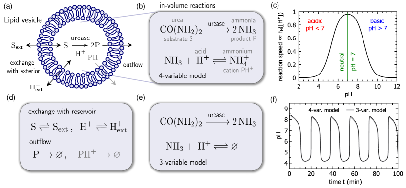
Figure 1: Schematic of the full four-variable and reduced three-variable reaction networks. (a) The enzyme (urease) assists conversion of the substrate S (urea) into product P (ammonia) in a lipid vesicle affected by varying acidity (hydrogen ion, H+). The substrate S and acid H+ exchange with the exterior of the vesicle, whereas the products P and PH+ (ammonium) are subjected to outflow from the vesicle (a,d); the ion form of product PH+ (reaction shown in gray) belongs only to the full reaction network. In-volume reactions occurring in the vesicle for (b) the full network, Eq. 1, and (e) the reduced network, Eq. 11. (c) The reaction speed of the urease-catalyzed step (1a) shows a bell-shaped dependence $f_{\textrm{H}}([\ce{H}^{+}])$ on $\ce{pH}=-\log_{10}([\ce{H+}]/$1\text{\,}\mathrm{M}$)$ with the maximum in a neutral medium ($\ce{pH}=7$), see Eqs. 2, 3 and 4. (f) pH oscillations obtained from the numerical solution of the four- and three-variable models, Eqs. 7 and 10, see also Fig. 2.

2 Reaction scheme and four-variable model

We start with the four-variable model of pH oscillations in the urea–urease reaction confined to lipid vesicle applied in our earlier study¹⁸ (Fig. 1a). The core of the reaction scheme consists of two reactions that occur within the reaction compartment:

$$\ce{S->[{k_{\mathrm{cat}}}][\text{\scriptsize\sf\>urease\;}]2P}\,,$$ (1a)

$$\ce{P+H+<=>[k_{2}][k_{2r}]PH+}\,.$$ (1b)

Reaction (1a) describes the enzyme-assisted hydrolysis of urea, CO(NH2)2, into ammonia, NH3, in the following denoted as substrate S and product P, respectively. Reaction (1b) accounts for the acidity of the medium and involves reversible conversion between the product P and its ion form PH+ (ammonium) with the corresponding rates ^{20, 7, 17} $k_{2}=$4.3\text{\times}{10}^{10}\text{\,}\mathrm{M}^{-1}\mathrm{s}^{-1}$$ and $k_{2r}=$24\text{\,}{\mathrm{s}}^{-1}$$. The effective speed $v([\ce{S}],[\ce{H+}])=k_{\mathrm{cat}}([\ce{S}],[\ce{H+}])[\ce{S}]$ of reaction (1a) depends on the concentrations [S] and [H+] of substrate and protons, respectively; or equivalently, on the level of $\ce{pH}=-\log_{10}([\ce{H+}]/$1\text{\,}\mathrm{M}$)$ and is given by the effective rate^{6, 14, 17}

$$k_{\mathrm{cat}}([\ce{S}],[\ce{H+}]) =k_{\mathrm{cat}}^{\mathrm{M}}([\ce{S}])f_{\mathrm{H}}([\ce{H+}])\,.$$ (2)

The first factor describes the dependence on the substrate as captured by the Michaelis–Menten kinetics,

$$k_{\mathrm{cat}}^{\mathrm{M}}([\ce{S}]) =\frac{v_{\mathrm{max}}}{K_{\mathrm{M}}+[\ce{S}]}$$ (3)

with the Michaelis–Menten constant^{12, 7, 17} $K_{\mathrm{M}}=$3\text{\times}{10}^{-3}\text{\,}\mathrm{M}$$. This implies that the reaction speed $v$ grows linearly with [S] at small $[\ce{S}]\ll K_{\mathrm{M}}$ and monotonically saturates at its maximum value $v_{\mathrm{max}}$ that would be attained in the absence of pH effects. The second factor implements the symmetric bell-shaped dependence of the reaction speed on the acidity (Fig. 1c, note the logarithmic scale):

$$f_{\mathrm{H}}([\ce{H+}]) =\frac{1}{1+[\ce{H+}]/K_{\mathrm{E1}}+K_{\mathrm{E2}}/[\ce{H+}]}\,,$$ (4)

which attains its maximum value $\max_{[\ce{H+}]}f_{\mathrm{H}}([\ce{H+}])=(1+2\sqrt{K_{\mathrm{E2}}/K_{\mathrm{E1}}})^{-1}$ at the hydrogen ion concentration $[\ce{H+}]=\sqrt{K_{\mathrm{E1}}K_{\mathrm{E2}}}$. For the constants chosen as ^{12, 7, 17} $K_{\mathrm{E1}}=$5\text{\times}{10}^{-6}\text{\,}\mathrm{M}$$ and $K_{\mathrm{E2}}=$2\text{\times}{10}^{-9}\text{\,}\mathrm{M}$$, it implies that the speed of reaction is maximum at the normal value of $\ce{pH}=7$, but is strongly suppressed when shifted from this optimal value to the regions of lower (acid) or higher (basic) pH.

The core reactions (1a) and (1b) are accompanied by the exchange with a reservoir and the decay of products (Fig. 1d); the reservoir acts as a buffer of substrate and pH, originally expressed by the reactions S <=>[k_S] S_ext and H+ <=>[k_H] H+_ext. This corresponds to the setting of the spatiotemporal master equation^{21, 22}; in particular, it relies on well-mixed conditions within the vesicle and in the reservoir and it neglects possible non-Markovian effects in the transport through the membrane ^{23, 24}. By assuming a sufficiently large reservoir such that the amounts of $\ce{S}_{\mathrm{ext}}$ and $\ce{H+}_{\mathrm{ext}}$ are changed only marginally, we consider the reservoir concentrations as fixed values $[\ce{S}_{\mathrm{ext}}]$ and $[\ce{H+}_{\mathrm{ext}}]$. The exchange reactions are then effectively replaced by

$$\ce{S<=>[k_{\mathrm{S}}][{k_{\mathrm{S}}[\ce{S}_{\mathrm{ext}}]}]\varnothing}\qquad\text{and}\qquad\ce{H+<=>[k_{\mathrm{H}}][k_{\mathrm{H}}{[\ce{H+}_{\mathrm{ext}}]}]\varnothing}\,.$$ (5)

The formulation of the reaction scheme is completed by specifying the decay of products or their outflow out of the reaction compartment by the reactions

$$\ce{P->[k]\varnothing}\qquad\text{and}\qquad\ce{PH+->[k]\varnothing}\,.$$ (6)

The set of reaction rate equations that corresponds to reactions (1), (5) and (6) reads:

$$\frac{d[\ce{S}]}{dt} =-k_{\mathrm{cat}}([\ce{S}],[\ce{H+}])[\ce{S}]+k_{\mathrm{S}}([\ce{S}_{\mathrm{ext}}]-[\ce{S}])\,,$$ (7a)

$$\frac{d[\ce{H+}]}{dt} =k_{2r}[\ce{PH+}]-k_{2}[\ce{P}][\ce{H+}]+k_{\mathrm{H}}([\ce{H+}_{\mathrm{ext}}]-[\ce{H+}])\,,$$ (7b)

$$\frac{d[\ce{P}]}{dt} =2k_{\mathrm{cat}}([\ce{S}],[\ce{H+}])[\ce{S}]+k_{2r}[\ce{PH+}]-k_{2}[\ce{P}][\ce{H+}]-k[\ce{P}]\,,$$ (7c)

$$\frac{d[\ce{PH+}]}{dt} =k_{2}[\ce{P}][\ce{H+}]-k_{2r}[\ce{PH+}]-k[\ce{PH+}]\,,$$ (7d)

which we will refer to as four-variable model in the following.

Focusing on the oscillatory regime, we stick to the parameter values used previously ¹⁸. Thus, the rates of urea and proton transport correspond to $k_{\mathrm{S}}=$1.4\text{\times}{10}^{-3}\text{\,}{\mathrm{s}}^{-1}$$ and $k_{\mathrm{H}}=$9\text{\times}{10}^{-3}\text{\,}{\mathrm{s}}^{-1}$$, respectively; the outflow rates of both products are set to $k=k_{\mathrm{S}}$. For the maximum speed we use the value $v_{\mathrm{max}}=$1.85\text{\times}{10}^{-4}\text{\,}\mathrm{M}\,\mathrm{s}^{-1}$$, which corresponds to an urea concentration of $50\text{\,}\mathrm{U}$. The external concentrations are fixed to $[\ce{S}_{\mathrm{ext}}]=$3.8\text{\times}{10}^{-4}\text{\,}\mathrm{M}$$ and $[\ce{H+}_{\mathrm{ext}}]=$1.3\text{\times}{10}^{-4}\text{\,}\mathrm{M}$$ and the initial concentrations inside the vesicle are $[\ce{S}]_{0}=$5\text{\times}{10}^{-5}\text{\,}\mathrm{M}$$ and $[\ce{H+}]_{0}=${10}^{-5}\text{\,}\mathrm{M}$$.

For these parameters, the four-variable model [Eq. 7] shows oscillatory behavior in the concentrations $[\ce{S}]$, $[\ce{H+}]$, $[\ce{P}]$ and $[\ce{PH+}]$ as exemplified in Fig. 2; note the logarithmic scale in panels (a) and (b). This evolution of the concentrations essentially reproduces that of the corresponding molecular populations in the large-vesicle limit, reported in Fig. 2 of Ref. 18; the periodic variation of the pH level, roughly between $3.5$ and $8.5$, reflects the behavior of [H+] and is shown in Fig. 1f. The concentrations of $\ce{H+}$ and $\ce{P}$ oscillate in anti-phase over four orders of magnitude, and the evolution of $[\ce{S}]$ and $[\ce{PH+}]$ shows the same periodic behavior, but with a much smaller amplitude, Fig. 2b.

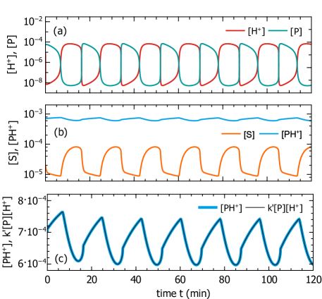
Figure 2: Evolution of the concentrations of [H+], [P], [S], and [PH+] in $\mathrm{M}$ from the numerical solution of the four-variable model, Eq. 7, on logarithmic scales (panels (a) and (b)). Panel (c) shows the behaviour of [PH+] (blue line) on linear scales, which coincides with the combination $k^{\prime}[\ce{P}][\ce{H+}]$ (thin black line), see Eq. 9.

3 Quasi-steady state approximation for PH+

Aiming at a characterization of the limit cycle of the urea–urease oscillator, we will first pursue a dimensional reduction of the dynamical system by elimination of inessential variables. Then, we will identify the actual degrees of freedom of the system and show that the dynamical system is effectively a two-dimensional one. In our previous work ¹⁸, starting from the four-variable model [Eq. 7], we applied the quasi-steady-state approximation (QSSA) simultaneously to the variables $[\ce{PH+}]$ and $[\ce{P}]$ in an ad hoc fashion. Here, we follow a more general and systematic approach, yielding more accurate reduced models and, particularly, also their regimes of validity. The model reduction occurs in two steps: In the first step, we eliminate $[\ce{PH+}]$, which leads to a three-variable model; this step is common to all models considered below. In the second step, we aim at a further reduction to two variables by eliminating $[\ce{P}]$, which can be performed in different ways leading to distinct models.

3.1 Reduction to three variables

By inspection of Fig. 2, we can draw two important conclusions. First, the concentration of the ion form of the product is larger than all other concentrations, $[\ce{PH+}]\gg[\ce{S}],[\ce{H+}],[\ce{P}]$. Second, the relative variation of $[\ce{PH+}]$ is smaller than those of the other concentrations, which suggests to approximate $[\ce{PH+}](t)$ by a constant. However, enforcing $[\ce{PH+}](t)=\mathrm{const}$ in Eq. 7, and thus $[\ce{P}](t)\,[\ce{H+}](t)=\mathrm{const}$, would turn the pH oscillations into a simple relaxation [Eq. 7b]. Instead, we observe that there exist well-separated timescales ^{25, 26}: the fast species $\ce{PH+}$ adjusts quickly, on the scale of $(k_{2r}+k)^{-1}=$4.2\text{\,}\mathrm{m}\mathrm{s}$$, to the slowly evolving concentrations of $\ce{P}$ and $\ce{H+}$, which vary on the scale of several minutes. This justifies to perform a QSSA for $\ce{PH+}$ by rearranging Eq. 7d into

$$[\ce{PH+}]=-(k_{2r}+k)^{-1}\,\frac{d[\ce{PH+}]}{dt}+k^{\prime}[\ce{P}][\ce{H+}]\,,\qquad k^{\prime}=\frac{k_{2}}{k_{2r}+k};$$ (8)

and neglecting the first term on the r.h.s., which yields the relation

$$[\ce{PH+}](t)=k^{\prime}[\ce{P}](t)\,[\ce{H+}](t)$$ (9)

with $k^{\prime}=$1.8\text{\times}{10}^{9}\text{\,}\mathrm{M}^{-1}$$ for the rates given above. The high accuracy of this approximation is corroborated by Fig. 2c, which shows that the temporal behavior of both sides of Eq. 9 coincides at all times, although none of the involved concentrations remains constant. Making use of Eq. 9 in Eqs. 7b and 7c, we arrive at a reduced model that employs only three variables:

$$\frac{d[\ce{S}]}{dt} =-k_{\mathrm{cat}}([\ce{S}],[\ce{H+}])[\ce{S}]+k_{\mathrm{S}}([\ce{S}_{\mathrm{ext}}]-[\ce{S}])\,,$$ (10a)

$$\frac{d[\ce{H+}]}{dt} =-kk^{\prime}[\ce{P}][\ce{H+}]+k_{\mathrm{H}}([\ce{H+}_{\mathrm{ext}}]-[\ce{H+}])\,,$$ (10b)

$$\frac{d[\ce{P}]}{dt} =2k_{\mathrm{cat}}([\ce{S}],[\ce{H+}])[\ce{S}]-kk^{\prime}[\ce{P}][\ce{H+}]-k[\ce{P}]\,.$$ (10c)

Note that while simplifying Eq. 10c, in accord with the above reasoning, we could have neglected the last term, $-k[\ce{P}]$. Indeed, the assumption $[\ce{PH+}]\gg[\ce{P}]$ together with Eq. 9 is equivalent to the requirement $k^{\prime}[\ce{H+}]\gg 1$. As independently confirmed by a previous study ¹⁷, this is a reasonable simplification for modeling pH oscillations. However, to analyze the dynamics in the whole phase plane and to keep the predictions of the reduced models as close as possible to those of the original four-variable model, we retain this term.

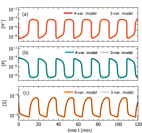
Figure 3: Comparison of the solutions of the four- and three-variable models given by Eqs. 7 and 10, respectively. The panels show the evolution of the concentrations of (a) acid [H+], (b) product [P], (c) and substrate [S]. The comparison of the corresponding pH levels is shown in Fig. 1f.

The dynamical system in Eq. 10 can be interpreted as the reaction rate equations of the following effective system of in-volume reactions (Fig. 1e):

$$\ce{S->[{k_{\mathrm{cat}}}][\text{\scriptsize\sf\>urease\;}]2P}\,,\qquad\ce{P+H+->[kk^{\prime}]\varnothing}\,,$$ (11)

amended by the exchange reactions (5) of S and H+ with the reservoir and the decay of P, see the first reaction in Eq. 6 (Fig. 1d). Thus, the product P has two channels to escape from the vesicle: directly and after protonation with an effective rate. In the original reaction scheme involving four species, the second channel exists indirectly, via escape of PH+.

We also note that despite relation (9) is fulfilled with high accuracy, the evolutions described by the three- and four-variable models are not identical (Figs. 1f and 3). Slight quantitative differences in the predictions of the two models are visible for P and pH (and, equivalently, for $[\ce{H+}]$). Interestingly, whereas the deviations are tiny for pH, they are more pronounced for P, yet eventually less important because we are generally not interested in the dynamics of the product. What is essential is that the reduced system (10) preserves not only all qualitative features of the four-variable model, but it remains quantitatively reliable in predicting the period of the oscillations. Thus, the three-variable model (10) serves as a highly accurate approximation.

3.2 Reduction to two variables

The further reduction of the three-variable model to two species by means of a QSSA for $[\ce{P}]$ appears less justified than the elimination of $[\ce{PH+}]$, as we will see below. Instead, we shall put forward a solution that yields an essentially exact reduction. It combines a scale separation argument and the condition in Eq. 9. As noted above, $[\ce{PH+}](t)$ oscillates slowly and with a relative amplitude of about 10% (Fig. 2c). In contrast, $[\ce{P}](t)$ and $[\ce{H+}](t)$ vary over four orders of magnitude on the same time scale (Fig. 3) and their logarithms oscillate very similarly, but in antiphase (Fig. 2a). Taking time derivatives, these observations suggest that the r.h.s. of the relation

$$\frac{d}{dt}\log([\ce{P}](t))+\frac{d}{dt}\log([\ce{H+}](t))=\frac{d}{dt}\log([\ce{PH+}](t)])$$ (12)

is negligible, which implies the approximate, yet accurate constraint

$$[\ce{P}](t)\,[\ce{H+}](t)\approx\mathrm{const}$$ (13)

and thus a tight coupling of the dynamics of $[\ce{P}](t)$ and $[\ce{H+}](t)$.

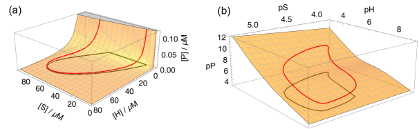
Figure 4: Phase plot of the limit cycle (red) of the three-variable model, Eq. 10, using linear (a) and logarithmic (b) scales. The surface is given by Eq. 19, which represents the constraint, Eq. 13. The black line is the orthogonal projection of the limit cycle to the plane $\ce{pP}=4$ and $[\ce{P}]=0$, respectively. In panel (b), we use the symbols $\ce{pX}=-\log_{10}([\ce{X}]/$1\text{\,}\mathrm{M}$)$ for $X=\ce{S},\ce{H+},\ce{P}$; note that small values of, e.g., pS correspond to large concentrations $[\ce{S}]$.

Figure 4 provides a visualization of the constraint in a three-dimensional phase plot of the three-variable model (10). First, we note that the structure of the limit cycle is not well resolved on linear scales (panel (a)), especially at small concentrations of $[\ce{H+}]$ (high pH). However, utilizing logarithmic scales, the structure of the limit cycle is uniformly well exhibited in the whole range of values (panels b). This observation is another indication that the oscillator studied here behaves differently than the conventional examples of pH oscillators ³. Second, one observes clearly that the dynamics in the three variables $[\ce{S}]$, $[\ce{H+}]$, and $[\ce{P}]$ is tightly confined to a two-dimensional manifold of roughly hyperbolic shape in the linear representation, see Eq. 13. The constraining manifold simplifies approximately to a plane in the logarithmic representation, which is tilted against all three coordinate axes; in particular, it deviates strongly from any plane given by a constant value of $[\ce{P}]$. This fact signifies clearly that the naive orthogonal projection of the phase flow to such a plane for the elimination of the variable $[\ce{P}]$ would be a poor approximation of the true dynamics; an issue we will expand on below (Section “Failure of QSSA for the product”).

Equipped with these insights, we proceed to eliminate the variable $\ce{P}$ from the three-dimensional model. For clarity of the subsequent analysis, we switch to dimensionless variables $s(t):=[\ce{S}](t)/[\ce{S}_{\textrm{ext}}]$, $h(t):=[\ce{H+}](t)/[\ce{H+}_{\textrm{ext}}]$, and $p(t):=k^{\prime}\,[\ce{P}](t)$, which turns Eq. 10 into

$$\frac{ds}{dt} =-k_{\mathrm{cat}}(s,h)\,s+k_{\mathrm{S}}\,(1-s)\,,$$ (14a)

$$\frac{dh}{dt} =-k\,p\,h+k_{\mathrm{H}}\,(1-h)\,,$$ (14b)

$$\frac{dp}{dt} =2\,\alpha_{\textrm{S}}\,k_{\mathrm{cat}}(s,h)\,s-\alpha_{\textrm{H}}\,k\,p\,h\,u(h)\,,$$ (14c)

where $\alpha_{\textrm{S}}:=k^{\prime}[\ce{S}_{\textrm{ext}}]$, $\alpha_{\textrm{H}}:=k^{\prime}[\ce{H+}_{\textrm{ext}}]$, and $u(h):=1+(\alpha_{\textrm{H}}h)^{-1}$. In terms of these variables, we rewrite Eq. 13 as

$$p(t)\frac{dh(t)}{dt}+\frac{dp(t)}{dt}h(t)\approx 0\,.$$ (15)

After substitution of the time derivatives using Eqs. 14b and 14c, the constraint assumes the form of a quadratic equation in $p=p(s,h)$,

$$p^{2}+b(h)\,p-c(s,h)=0\,,$$ (16)

with the dimensionless coefficients

$$b(h) =\alpha_{\textrm{H}}\,h\,u(h)+(1-h^{-1})\,k_{\mathrm{H}}/k$$ (17)

and

$$c(s,h) =\frac{2\,\alpha_{\textrm{S}}\,k_{\mathrm{cat}}(s,h)}{k}s\geq 0\,.$$ (18)

Equation 16 possesses two roots, $p_{\pm}(s,h)$, and selecting the positive solution, $p(s,h)\geq 0$ for all $s,h\geq 0$, we obtain

$$p(s,h)=\frac{b(h)}{2}+\frac{1}{2}\sqrt{b(h)^{2}+4c(s,h)}\,.$$ (19)

In particular, the time evolution of the rescaled concentration $[\ce{P}]$ of products is enslaved to the evolution of $[\ce{S}]$ and $[\ce{H+}]$ and is given by $p(t)=p(s(t),h(t))$.

This solution for $p(t)$ allows us to eliminate $p(t)$ as a variable from the three-variable model in Eq. 14. In particular, one verifies that Eq. 14c is automatically satisfied and can be dropped. The remaining Eqs. 14a and 14b yield the two-variable model:

$$\frac{ds}{dt} =F(s,h):=-k_{\mathrm{cat}}(s,h)\,s+k_{\mathrm{S}}\,(1-s)\,,$$ (20a)

$$\frac{dh}{dt} =G(s,h):=-k\,p(s,h)\,h+k_{\mathrm{H}}\,(1-h)\,,$$ (20b)

where $p(s,h)$ is defined by relation (19) with the coefficients $b(s,h)$ and $c(s,h)$ given by Eqs. 17 and 18. We stress that Eq. 19 is a consequence of Eq. 13 or, equivalently, Eq. 15. The two-variable model [Eq. 20 with Eq. 19] is thus a virtually exact representation of the three-variable model (10). However, differently from the latter, Eq. 20 does not have a meaningful interpretation as rate equations of a system of effective reactions unless one accepts $k\,p(s,h)$ as an effective decay rate of $\ce{H+}$. Since the introduction of nonelementary rates as a result of reduction on the deterministic level may lead to significant quantitative and even qualitative errors in stochastic simulations,^{27, 28} it is favorable to use the three-variable alternative as a stochastic model.

4 Limit cycle and structure of the phase flow

4.1 Nullclines

General properties of the limit cycle can be understood from the geometric structure of the phase flow $(F(s,h),G(s,h))$ of a dynamical system. Helpful characteristics specifying the structure of the phase flow or phase portrait are nullclines. For the two-variable model (20), the $\ce{S}$ and $\ce{H+}$ nullclines are defined by the conditions $F(s,h)=0$ and $G(s,h)=0$, respectively. By construction, on a given nullcline the flow is perpendicular to the axis of the corresponding variable. The intersection of all nullclines defines all fixed points of the phase flow, which represent the steady state solutions of Eq. 20, i.e., the points where all time derivatives vanish. For the present two-variable model, both nullclines can be obtained analytically.

The $\ce{S}$ nullcline is calculated by putting $F(s,h)=0$ in Eq. 20a, which on account of Eq. 2 leads to a quadratic equation in $s$:

$$s^{2}+\beta(h)s-\bar{K}_{\mathrm{M}}=0\quad\text{with}\quad\beta(h):=\bar{K}_{\mathrm{M}}-1+\bar{v}_{\mathrm{max}}f_{\mathrm{H}}(h)\,,$$ (21)

where $\bar{v}_{\mathrm{max}}:=v_{\mathrm{max}}/(k_{\mathrm{S}}[\ce{S}_{\mathrm{ext}}])$, $\bar{K}_{\mathrm{M}}:=K_{\mathrm{M}}/[\ce{S}_{\mathrm{ext}}]$ and $f_{\mathrm{H}}(h)$ is given by Eq. 4. Out of the two roots $s_{\pm}(h)$, only the one describing non-negative substrate concentration is physically relevant, thus yielding the $\ce{S}$ nullcline,

$$s_{\mathrm{S}}^{\mathrm{nc}}(h)=s_{+}(h):=-\frac{\beta(h)}{2}+\frac{1}{2}\sqrt{\beta(h)^{2}+4\bar{K}_{\mathrm{M}}}\,.$$ (22)

Note that the dependence of $s_{\mathrm{S}}^{\mathrm{nc}}(h)$ on $h$ inherits its shape directly from Eq. 4. Its maximum is located at $h_{\textrm{m}}=\sqrt{K_{\textrm{E1}}K_{\textrm{E2}}}/[\ce{H+}_{\textrm{ext}}]$ as determined from the condition $s_{+}^{\prime}(h_{m})=0$, which is found to be equivalent to $f_{\textrm{H}}^{\prime}(h_{\textrm{m}}[\ce{H+}_{\textrm{ext}}])=0$.

To obtain the H+ nullcline, we set $G(s,h)=0$ in Eq. 20b and, using the definition of $p(s,h)$, after some tedious algebra, we arrive at the intermediate relation,

$$2\kappa k_{\mathrm{cat}}(s,h)s=k_{\mathrm{H}}(1-h)u(h)$$ (23)

with $\kappa=\alpha_{\textrm{S}}/\alpha_{\textrm{H}}=[\ce{S}_{\mathrm{ext}}]/[\ce{H+}_{\mathrm{ext}}]$. More straightforwardly, we can derive this result by making use of Eq. 15, which implies that $dh/dt=0$ is equivalent to $dp/dt=0$ for $p(t),h(t)>0$: to this end, we set to zero the time derivative in Eq. 10c, solve for

$$kp(s,h)h=\frac{2\kappa k_{\mathrm{cat}}(s,h)}{u(h)}\,s\,,$$ (24)

and substitute it in Eq. 20b. Finally, inserting the definition of $k_{\mathrm{cat}}(s,h)$, Eq. 2, into the intermediate equation for $s$ leads us to the H+ nullcline,

$$s_{\mathrm{H}}^{\mathrm{nc}}(h)=\bar{K}_{\mathrm{M}}\left[\frac{2\kappa k_{\textrm{S}}\bar{v}_{\mathrm{max}}f_{\mathrm{H}}(h)}{k_{\mathrm{H}}(1-h)u(h)}-1\right]^{-1}\,.$$ (25)

4.2 Phase flow

The origin of the limit cycle is easily understood from the phase portrait of the two-dimensional dynamical system, Eq. 20, and the associated nullclines, Eqs. 22 and 25. As mentioned earlier, a remarkable feature of this system is that the structure of the phase flow is best unveiled on logarithmic scales—in contrast to conventional examples of oscillators. Therefore, instead of the original variables $s$ and $h$, we will use $\ce{pS}$ and $\ce{pH}$ as axes of the phase plane. The phase flow of the two-variable model together with its nullclines and the limit cycle are shown in Fig. 5a. For the parameters considered here, the nullclines intersect only in a single, repelling fixed point enclosed by the limit cycle. The limit cycle was obtained from the numerical solution of $ds/dt=F(s,h)$ and $dh/dt=G(s,h)$ after a sufficiently long initial relaxation time.

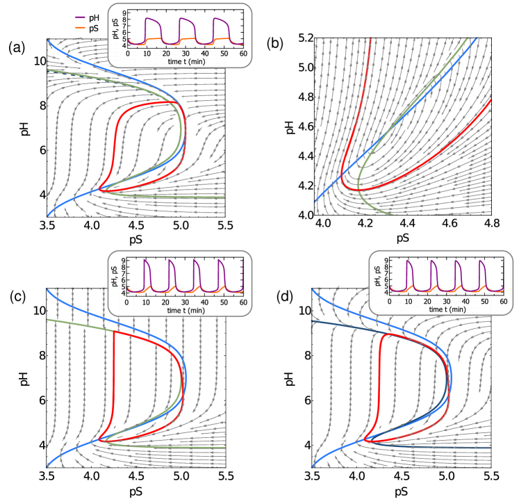
Figure 5: Phase flows (grey arrows) and limit cycles (red lines) in the pS-pH plane for the two-variable models obtained from two different reduction schemes of the three-variable model [Eq. 10]: (a)  accurate model [Eq. 20] from the exact elimination of the product $p$; (b)  close-up of the vicinity of the fixed point at $(\ce{pS}_{*},\ce{pH}_{*})\approx(4.31,4.57)$ shown in (a); (c)  model in Eq. 26 from imposing the QSSA for $p(t)$; (d)  model in Eq. 39 from explicitly accounting for the water ionization, Eq. 36, and then imposing the QSSA on the product, this model corresponds to the two-variable model studied by Bánsági and Taylor ¹⁷. The S (blue lines) and H+ (green lines) nullclines are the same for the models in (a)–(c) and are given by Eqs. 22 and 25, respectively. Including the water ionization leads to a slight shift of the H+ nullcline from the green line to the dashed blue line in (a) and to the dark blue line in (d), Eq. 40.

Qualitatively, the shape of the limit cycle is determined by the nullclines and the two-dimensional flow field $(F(s,h),G(s,h))$. The S nullcline (Eq. 22, blue line in Fig. 5a) has a rotated bell shape, inherited from the function $f_{\textrm{H}}([\ce{H+}])$ (see Eq. 4 and Fig. 1f); and the H+ nullcline (Eq. 25, green line in Fig. 5a) is of a reversed s-like shape. The requirement on the flow field that, at any point of the nullclines, there is no motion along the corresponding direction means that the flow on the S nullcline can only point along the pH direction (vertical arrows) and on the H+ nullcline along the pS direction (horizontal arrows). In the high pH regime, both nullclines run closely together such that the H+ nullcline pushes the flow towards the S nullcline. This causes a channeling of the flow between the two nullclines towards the apex of the S nullcline, $(\ce{pS},\ce{pH})\approx(5,7)$, where $s_{\mathrm{S}}^{\mathrm{nc}}(h)$ attains its maximum value. There, the flow points downwards, along the pH axis, and is tightly restricted with respect to pS (i.e., horizontally), concomitantly the pH value drops rapidly. All phase trajectories, irrespective of their starting point, eventually approach this apex point arbitrarily closely and follow the S nullcline for a moment, which essentially defines a piece of the limiting trajectory (limit cycle, red line). After this point, the S nullcline bends away from the vertical, but the trajectory keeps following the flow field and revolves around the fixed point until the orbit closes, which forms the limit cycle. Thus, the limit cycle is determined as the trajectory that starts in the apex of the S nullcline, where the curve attains its largest pS value.

The H+ and S nullclines, shown in Fig. 5a, have a single intersection point, defining a fixed point, which is enclosed by the limit cycle. The flow field in the vicinity of the fixed point (Fig. 5b) indicates that this fixed point acts as a repeller. This observation is in agreement with the Poincaré–Hopf theorem of indices ²⁹. It states that the index $I(\gamma)$ of any closed curve $\gamma$ equals the sum of the indices $I_{k}$ of all the enclosed fixed points, $I(\gamma)=\sum_{k}I_{k}$, where one assigns the index $I(\gamma)=+1$ to a periodic orbit $\gamma$, while the index of a saddle fixed point is $I=-1$ and the index of a node, a spiral (focus) or a center is $I=+1$. As a consequence, the limit cycle must enclose at least one fixed point (which must not be a saddle point). Moreover, the existence of a single repelling fixed point as in Fig. 5b automatically implies that it is either an unstable spiral or node. A more detailed stability analysis will be given below (Section ‘Fixed point and its stability’).

5 Failure of QSSA for the product

In the literature, it was suggested to apply the QSSA to the concentration $[\ce{P}]$ of products ^{17, 18}. Here we elaborate on the consequences of this approximation and show that although the nullclines remain the same as in the exact reduction scheme, it qualitatively changes the phase flow and significantly affects the oscillations. In hindsight, it is clear that generally such an approximation cannot be consistent with the QSSA for $[\ce{PH+}]$, which leads to the three-variable model, Eq. 11, and constrains the three-dimensional flow to a two-dimensional manifold as discussed above (Fig. 4).

This elimination scheme follows directly from Eq. 14 by enforcing the QSSA for $p(t)$. As has already been shown, setting $dp/dt=0$ in Eq. 14c yields expression (24) for the combination $kp(s,h)h$. Substituting it in Eq. 14b, we arrive at the model:

$$\frac{ds}{dt} =-k_{\mathrm{cat}}(s,h)s+k_{\mathrm{S}}(1-s)\,,$$ (26a)

$$\frac{dh}{dt} =-\frac{2\kappa k_{\mathrm{cat}}(s,h)}{u(h)}\,s+k_{\mathrm{H}}(1-h)\,.$$ (26b)

In our previous study,¹⁸ this model was used with $u(h)=1$ to qualitatively obtain the structure of the phase portrait exhibited by the numerical solution of the four-variable model. As earlier, the H+ nullcline corresponding to Eq. 26b follows simply by setting $dh/dt=dp/dt=0$ in Eqs. 14b and 14c and solving for $s(h)$. Expressing the combination $kph$ from the equation for $h$ and equating it with that from Eq. 24, we end up with the H+ nullcline identical to Eq. 25. The S nullcline is given by Eq. 22 due to the coincidence of the equations for $s$, cf. Eq. 20a and Eq. 26a.

By comparing the phase plots of the models given by Eq. 20 and Eq. 26, we immediately notice that although the nullclines of both models are the same, the flow fields in the upper half of the plots (large pH) are drastically different (Fig. 5a, c). In particular, the behavior of the flow field on the upper branch of the H+ nullcline described by Eq. 26 degenerates (Fig. 5c). By construction, the flow on the H+ nullcline has to point in the pS direction (horizontal arrows), meaning the absence of the pH (vertical) component of the flow field, $dh/dt=0$; the latter has to comply with the fact that $dh/dt$ has opposite signs above and below the nullcline. Closer inspection of the flow shows that, in contrast to model (20), the relative role of the vertical component of the flow field appears strongly overestimated by the QSSA such that the relation $|ds/dt|\ll|dh/dt|$ holds already slightly away from the nullcline. As a result of this improper balance of the two components, the flow field bends sharply near the H+ nullcline and follows it towards larger pS with a small velocity (Fig. 5c). In other words, the H+ nullcline acts as a virtual attractor, which is a qualitatively wrong picture as follows from the comparison with the flow of the accurate model (20) shown in Fig. 5a. Figure 5c reveals further that the limit cycle is formed in a qualitatively different way. In contrast to the accurate scenario, the shape of the limit cycle is now fully set by the upper branch of the H+ nullcline, which directly affects the oscillation behavior predicted by this model. The temporal oscillation patterns (insets of Fig. 5a,c) exhibit drastically different shapes. In particular, the ad-hoc model (26) exhibits a significantly shorter relaxation of the pH level (Fig. 5c) relative to the prediction of the accurate model (20). As a result, the oscillation period is found to be $12.68\text{\,}\mathrm{min}$ within model (26), which underestimates the reliable prediction of $17.59\text{\,}\mathrm{min}$ within model (20) by nearly $30\%$. We note further that model (26), which degenerates at high pH and fails to capture the rounded shape of the limit cycle, also overestimates the amplitude of the pH oscillations: it yields $\max(\ce{pH})-\min(\ce{pH})\approx 4.9$, which is to be compared to the value $4.0$ obtained within model (20).

We note that the model given by Eq. 26, and hence the QSSA for the product P, correspond to a special limit of the model given by Eq. 20. It follows from the exact solution for $p(s,h)$, see Eqs. 17, 18 and 19, under two separate conditions. First, one requires that $b(h)^{2}\gg 4c(s,h)$, which permits the expansion of the square root in Eq. 19,

$$p(s,h) \simeq-\frac{b(h)}{2}+\frac{|b(h)|}{2}\left(1+\frac{2c(s,h)}{b(h)^{2}}\right)$$

$$=\begin{cases}c(s,h)/b(h),&\text{if }b(h)>0\,,\\ -b(h),&\text{if }b(h)<0\,.\end{cases}$$ (27)

Second, if $\alpha_{\textrm{H}}hu(h)\gg(1-h^{-1})k_{\mathrm{H}}/k$ one can simplify $b(h)\simeq\alpha_{\textrm{H}}hu(h)>0$ yielding

$$p(s,h)=\frac{2\kappa k_{\mathrm{cat}}(s,h)}{khu(h)}s\geq 0\,.$$ (28)

We note that this result corresponds to setting $dp/dt=0$ in Eq. 14c.

Thus, the two assumptions leading to Eq. 28 define the regime of validity of the QSSA and essentially require that $b(h)$ is positive and large enough. As follows from Eq. 27, in the opposite regime $b<0$ and large $|b|$, the consistent approximation for $p(s,h)$ should be different. The border case, $b(h)=0$, occurs for $h=[\sqrt{(k_{\textrm{H}}+k)^{2}+4\alpha_{\textrm{H}}kk_{\textrm{H}}}-(k_{\textrm{H}}+k)]/(2\alpha_{\textrm{H}}k)$. For the parameters used here, $\alpha_{\textrm{H}}\approx$2\text{\times}{10}^{6}$\gg 1$ and $h\approx\sqrt{k_{\textrm{H}}/(\alpha_{\textrm{H}}k)}$, which corresponds to $\ce{pH}\approx 6.17$. This means that the approximation (28) is justified for a part of the oscillation period only, namely for $\ce{pH}\lesssim 6$ (then $h$ is large enough and $b(h)>0$), see inset of Fig. 5a. For the rest of the period, where $\ce{pH}\gtrsim 6$, the approximation Eq. 28 is not applicable. In this regime, either the above expansion fails completely (for $\ce{pH}\approx 6$, $b^{2}\ll 4c$) or $p$ is determined by a different relation than Eq. 28 (large values of pH, $b^{2}\gg 4c$, but $b<0$). These are the reasons that significantly restrict the validity of the QSSA for P and thus of the whole model given by Eq. 26. In particular, the preceding analysis explains why the model (26) exhibits a degeneracy and becomes unreliable when the pH level is neutral or basic ($\ce{pH}\gtrsim 6$).

6 Fixed points and stability analysis

For the characterization of the parameter regimes where oscillatory behavior is predicted, we shall determine the fixed points of the accurate model, Eq. 20, and analyse their stability. The problem does not admit for a simple analytic treatment in the whole pH range. However, noting that the fixed point giving rise to oscillations is located in the acid regime, we exploit that, for low pH values, Eq. 20 reduces to the more tractable model in Eq. 26. This approach is corroborated by Fig. 5: for the parameter set used, the models (20) and (26) display very similar flow fields for $\ce{pH}\lesssim 6$ (panels (a) and (c)). The S and H+ nullclines exhibit a single intersection, which is located in the acid regime, $\ce{pH}\approx 4.6$ (panels (a) and (b)); the intersection yields the fixed point of the flow, and the surrounding flow field indicates that it is an unstable one. We will now obtain an analytic expression for the fixed point, explore its stability and develop an overall picture of the possible equilibria.

6.1 Stability of equilibria and domain of oscillations

The fixed points $(s_{*},h_{*})$ of model (20), and also of model (26), with $p(s,h)$ given by either Eq. 19 or Eq. 28, respectively, are determined by the conditions

$$F(s_{*},h_{*}) =-k_{\mathrm{cat}}(s_{*},h_{*})\,s_{*}+k_{\mathrm{S}}\,(1-s_{*})=0\,,$$ (29a)

$$G(s_{*},h_{*}) =-k\,p(s_{*},h_{*})\,h_{*}+k_{\mathrm{H}}\,(1-h_{*})=0\,,$$ (29b)

or, equivalently, by $s_{*}:=s_{\mathrm{S}}^{\mathrm{nc}}(h_{*})=s_{\mathrm{H}}^{\mathrm{nc}}(h_{*})$, with the functions given in Eqs. 22 and 25. Generally, these equations admit more than a single solution. The nature of each obtained fixed point then follows from the corresponding linear stability problem.

Introducing the deviation $\bm{\epsilon}=(s-s_{*},h-h_{*})$ from the fixed point $(s_{*},h_{*})$ and linearizing the flow field, Eq. 20, around this point, one obtains the linear flow equation $d\bm{\epsilon}/dt=J(s_{*},h_{*})\bm{\epsilon}+O(\bm{\epsilon}^{2})$ with the Jacobian $J=\partial(F,G)/\partial(s,h)$, which is a $2\times 2$ matrix with elements $J_{11}=\partial F/\partial s$, $J_{12}=\partial F/\partial h$, $J_{21}=\partial G/\partial s$, $J_{22}=\partial G/\partial h$, evaluated for the solution at the point $(s_{*},h_{*})$. This linear ordinary differential equation is solved with the ansatz $\bm{\epsilon}\propto\exp(\lambda t)$, which leads to the characteristic polynomial $\lambda^{2}-(\operatorname{Tr}J)\,\lambda+\operatorname{Det}J=0$ in the growth rate $\lambda$. The two roots $\lambda_{\pm}$ are complex-valued if the discriminant $\Delta=(\operatorname{Tr}J)^{2}-4\operatorname{Det}J$ is negative, and real-valued otherwise. Recalling that $\operatorname{Det}J=J_{11}J_{22}-J_{12}J_{21}=\lambda_{+}\lambda_{-}$ and $\operatorname{Tr}J=J_{11}+J_{22}=\lambda_{+}+\lambda_{-}$, it follows that the flow near the fixed point under consideration is a saddle if $\operatorname{Det}J<0$. If $\operatorname{Det}J>0$, it is either a node ($\Delta>0$), a spiral (or focus) ($\Delta<0$), or a center ($\Delta=0$), as the border case. The nodes and spirals can be stable ($\operatorname{Tr}J<0$) or unstable ($\operatorname{Tr}J>0$). The conditions

$$\operatorname{Tr}J=0,\quad\operatorname{Det}J=0,\quad\text{and}\quad\Delta=0,$$ (30)

allow us to divide the parameter space into regions of sustained oscillations, stable steady states, and bistability.

Many of the reaction parameters are system specific and therefore remain fixed for the urea–urease reaction. What can be potentially changed in the experiment are the external concentrations $[\ce{S}_{\textrm{ext}}]$ and $[\ce{H+}_{\textrm{ext}}]$ and the reaction speed of the catalytic step, $v_{\textrm{max}}\propto[\ce{E}]$, which depends on the total concentration $[\ce{E}]$ of urease in the vesicle. Furthermore, the rates $k_{\textrm{H}}$ and $k_{\textrm{S}}$ are directly related to the experimentally relevant permeabilities of the membrane to the hydrogen ion H+ and urea S ^{9, 10}, and it was found in a theoretical study that these rates must satisfy certain conditions for the existence of oscillations ¹⁷. Here, we consider the ratio $\bar{K}_{\textrm{H}}=k_{\textrm{H}}/k_{\textrm{S}}$, which specifies the degree of differential transport through the membrane. In the following, we will present the overall classification of the type of behavior on the $\kappa$-$\bar{K}_{\textrm{H}}$ plane (recall that $\kappa=[\ce{S}_{\textrm{ext}}]/[\ce{H+}_{\textrm{ext}}]$) and then show how the domain of oscillations varies upon changing the parameters $\bar{v}_{\textrm{max}}=v_{\textrm{max}}/(k_{\textrm{S}}[\ce{S}_{\textrm{ext}}])$ and $\bar{K}_{\textrm{M}}=K_{\textrm{M}}/[\ce{S}_{\textrm{ext}}]$. Thereby, our analysis effectively covers the dependencies on $k_{\textrm{H}}$ and $k_{\textrm{S}}$ as well as on $[\ce{S}_{\textrm{ext}}]$, $[\ce{H+}_{\textrm{ext}}]$, and $[\ce{E}]$.

Calculating the elements of the Jacobian $J(s_{*},h_{*})$ from Eq. 20, we find after some algebra:

$$J_{11} =-k_{\textrm{S}}\frac{\bar{K}_{\textrm{M}}}{\bar{K}_{\textrm{M}}+s_{*}}\frac{1-s_{*}}{s_{*}}-k_{\textrm{S}}\,,$$ (31a)

$$J_{12} =k_{\textrm{S}}(1-s_{*})f_{\textrm{H}}(h_{*})z(h_{*})\,,$$ (31b)

$$J_{21} =-\frac{2k_{\textrm{S}}\alpha_{\textrm{S}}h_{*}}{\sqrt{b_{*}^{2}+4c_{*}}}\frac{\bar{K}_{\textrm{M}}}{\bar{K}_{\textrm{M}}+s_{*}}\frac{1-s_{*}}{s_{*}}\,,$$ (31c)

$$J_{22} =\frac{\alpha_{\textrm{S}}h_{*}}{\sqrt{b_{*}^{2}+4c_{*}}}\left[k_{\textrm{H}}\frac{1-h_{*}}{\alpha_{\textrm{S}}h_{*}}b^{\prime}_{*}+2J_{12}\right]-\frac{k_{\textrm{H}}}{h_{*}}\,,$$ (31d)

where $b_{*}=b(h_{*})$, $c_{*}=c(s_{*},h_{*})$ and $b^{\prime}_{*}=db(h_{*})/dh$ are evaluated at the fixed point $(s_{*},h_{*})$ and we have abbreviated $z(h_{*}):=\bar{K}_{\textrm{E1}}^{-1}-\bar{K}_{\textrm{E2}}/h_{*}^{2}$ with $\bar{K}_{\textrm{E1}}=K_{\textrm{E1}}/[\ce{H+}_{\textrm{ext}}]$, $\bar{K}_{\textrm{E2}}=K_{\textrm{E2}}/[\ce{H+}_{\textrm{ext}}]$. These expressions together with the conditions in Eq. 30 and the fixed point, Eq. 29, define the boundaries of the various types of fixed point behavior in the $\kappa$-$\bar{K}_{\textrm{H}}$ plane (Fig. 6a). Setting $\bar{v}_{\textrm{max}}=347$ and $\bar{K}_{\textrm{M}}=7.90$ and selecting each of the conditions in Eq. 30, we have numerically determined the values of $\bar{K}_{\textrm{H}}$, $s_{*}$, and $h_{*}$ that satisfy the respective condition and Eq. 29 for a range of prescribed values of $\kappa$.

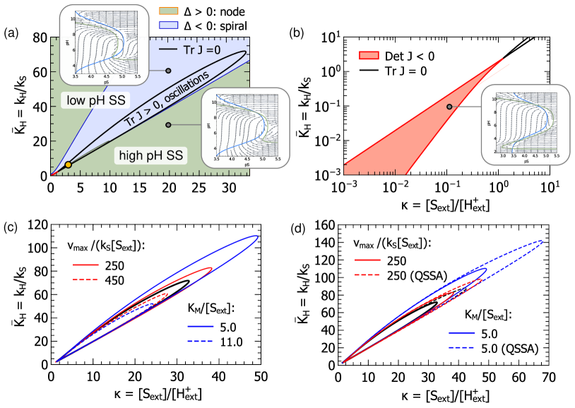
Figure 6: Stability diagrams in the $\kappa$-$\bar{K}_{\textrm{H}}$ plane plane, shown for $\bar{v}_{\textrm{max}}=347$ and $\bar{K}_{\textrm{M}}=7.9$ if not stated differently.  (a) Domains with a single fixed point of different behavior, leading to self-sustained oscillations (region within the thick black line, $\operatorname{Tr}J>0$), or steady states (SS) at low or high pH values (region outside of the thick black line, $\operatorname{Tr}J<0$). The latter are approached via damped oscillations (spiral, shaded blue region, $\Delta<0$) or without oscillations, in a fully overdamped fashion (node, shaded green region, $\Delta>0$). The domains are delimited by the conditions $\operatorname{Tr}J=0$ (thick black line) and $\Delta=0$ (center, thin violet line). The orange disk indicates the set of parameters used for all other results in this work, $\kappa=2.92$, $\bar{K}_{\textrm{H}}=6.43$. The insets show phase plots and the location of the nullclines at two exemplary high and low pH SS, at $(\kappa,K_{\textrm{H}})=(20,30)$ and $(20,60)$.  (b) Close-up of the bottom-left corner of panel (a), revealing the domain of bistability ($\operatorname{Det}J<0$) with two attractive fixed points and a saddle in between, as illustrated in the inset corresponding to $(\kappa,\bar{K}_{\textrm{H}})=(0.1,0.1)$.  (c) Domain of oscillation for different values of $v_{\textrm{max}}$ and $K_{\textrm{M}}$. The thick solid black line is the same as in panel (a) and serves as reference.  (d) Comparison of the predictions of the accurate model, Eq. 20, (solid lines) with those from invoking the QSSA for the product, Eq. 26 (dashed lines). The thick solid black line is the reference line as in panel (a) and the dashed black line corresponds to its QSSA counterpart.

We find that in almost the whole plane, except for a small region at low values of $\kappa$ and $\bar{K}_{\textrm{H}}$ (lower left corner of the plot), there is a single fixed point with $\operatorname{Det}J>0$, meaning that the fixed point is either a node (green shaded, $\Delta>0$) or a spiral (blue shaded, $\Delta<0$), separated by the border case of a center (thin blue line, $\Delta=0$). Nearly the whole domain of oscillations ($\operatorname{Tr}J>0$, enclosed by the thick black line) is characterized by an unstable spiral as fixed point. Merely near the lower-$\bar{K}_{\textrm{H}}$ border for $1.5\lesssim\kappa\lesssim 10$, there is a narrow stripe of unstable nodes. It indicates that, although less frequently observed than the spiral along with the spiral, an unstable node is also a possible type of fixed point that can be enclosed by a limit cycle, in accordance with the Poincaré–Hopf theorem.

The regions above (higher $\bar{K}_{\textrm{H}}$) and below (lower $\bar{K}_{\textrm{H}}$) of the domain of oscillations exhibit steady states with low and high pH levels, respectively. Here, $\operatorname{Tr}J<0$ and the corresponding steady state is approached either via damped oscillations (blue shading) or aperiodically in an overdamped fashion (green shading); the domain of high pH steady states is, however, predominantly overdamped. The corresponding fixed points in the pS-pH plane (see insets of Fig. 6a) are located either below (low pH steady state) or above (high pH steady state) the neutral $\ce{pH}=7$ level; the latter is set by the apex point of the S nullcline. Therefore, they can be referred to as the acid ($\ce{pH}<7$) and base ($\ce{pH}>7$) steady states, respectively.

A domain of bistability exists at small values $\kappa\lesssim 1$ and $\bar{K}_{\textrm{H}}\lesssim 1$, which is better resolved on logarithmic scales (Fig. 6b, red shading). In this domain, the fixed point discussed so far is a saddle ($\operatorname{Det}J<0$), and the domain is delimited by the condition $\operatorname{Det}J=0$ (dark red lines); it touches the domain of oscillations ($\operatorname{Tr}J=0$, solid black line) at the largest values of $\kappa$ and $\bar{K}_{\textrm{H}}$ with $\operatorname{Det}J=0$ (top-right corner of Fig. 6b). The saddle point is accompanied by two stable nodes, acting as attractors, which is exemplarily shown by the phase plot for the point $(\kappa,\bar{K}_{\textrm{H}})=(0.1,0.1)$ in the inset of Fig. 6b. The S and H+ nullclines intersect in three different fixed points, the outermost fixed points define the low (acid) or high (base) pH steady states. Thus, which of the two states the system evolves to depends solely on the initial state. This completes the overall structure of the possible equilibria of the urea–urease reaction. Being interested in oscillatory behavior, we will now discuss how the detected domain of oscillations transforms upon changing other control parameters.

Figure 6c illustrates what happens to the domain of oscillations upon changing the parameters $\bar{v}_{\textrm{max}}$ and $\bar{K}_{\textrm{M}}$. The curve shown by thick black line reproduces the domain of oscillations from Fig. 6a, for $v_{\textrm{max}}=347$ and $\bar{K}_{\textrm{M}}=7.90$, and serves as a reference. First, changing only the reaction speed $\bar{v}_{\textrm{max}}$ (for $\bar{K}_{\textrm{M}}=7.90$ fixed) leads to an elongation of the domain for smaller ($\bar{v}_{\textrm{max}}=250$, solid red line) and a a shrinking for larger ($\bar{v}_{\textrm{max}}=250$, dashed red line) values of $\bar{v}_{\textrm{max}}\propto[E]$; under these changes, the domain keeps its elongated, petal-like shape oriented approximately along the line $\bar{K}_{\textrm{H}}\approx 2\kappa$. Second, we stick to the value $v_{\textrm{max}}=347$ and obtain a similar effect upon changing $\bar{K}_{\textrm{M}}$: the domain of oscillations elongates at lower ($K_{\textrm{M}}=5$, solid blue line) and shrinks at higher ($K_{\textrm{M}}=11$, dashed blue line) values of $\bar{K}_{\textrm{M}}$. In all these situations, the elongation and shrinking affects the rounded end of the petal (maximal values of $\kappa$ and $\bar{K}_{\textrm{H}}$ for oscillations), while it remains unchanged at its cusp end ($\kappa\approx\bar{K}_{\textrm{H}}\approx 1$).

We now also show that the accuracy of the model plays an important role for correctly obtaining the boundaries of the oscillation domain. We compare the predictions of the accurate model (20) with those based on the QSSA for the product, Eq. 26. Note that for model Eq. 26, the equation for $h$ is different and the elements $J_{21}$ and $J_{22}$ of the Jacobian differ. Evaluating the derivatives of the r.h.s. of Eq. 26b, we obtain

$$J_{21} =-\frac{2k_{\textrm{S}}\kappa}{u(h_{*})}\frac{\bar{K}_{\textrm{M}}}{\bar{K}_{\textrm{M}}+s_{*}}\frac{1-s_{*}}{s_{*}}\,,$$ (32a)

$$J_{22} =\frac{1}{u(h_{*})}\left[k_{\textrm{H}}\frac{1-h_{*}}{h_{*}}+2\kappa J_{12}\right]-\frac{k_{\textrm{H}}}{h_{*}}\,.$$ (32b)

Alternatively, these expressions follow from Eqs. 31c and 31d by passing to the limit of large and positive $b(h_{*})$, as discussed for Eqs. 27 and 28, so that $\sqrt{b_{*}^{2}+4c_{*}}\simeq b(h_{*})\simeq\alpha_{\textrm{H}}h_{*}u(h_{*})$ and $db(h_{*})/dh\simeq\alpha_{\textrm{H}}$. In Fig. 6d, we compare the predictions for the domain of oscillations resulting from the accurate and the QSSA-based models for a few values of $v_{\textrm{max}}$ and $\bar{K}_{\textrm{M}}$. We find that in all cases the QSSA significantly overestimates the size of the domain of oscillations. The domain boundaries remain close for the two models if $\kappa$ is small, but they start to deviate as $\kappa$ grows. The root of this deficiency of the QSSA-based model lies in the restricted applicability of the QSSA to low $\ce{pH}$ values: while moving from lower to higher values of $\kappa$ along the upper (high-$\bar{K}_{\textrm{H}}$) part of the boundary of the petal-shaped domain, the fixed point lies initially in the low pH regime, but gradually shifts towards higher pH levels. Upon reaching the rounded end of the petal and following the lower part of the boundary, the pH value (and thus $h_{*}$) reaches and then goes beyond the point where $b(h_{*})=0$ (in case of the bold black reference curve, this happens at $\ce{pH}\approx 6.17$) and the QSSA model fails.

6.2 Analytic results for the fixed point governing the oscillations

The fixed point $(s_{*},h_{*})$ is determined by the condition $s_{*}:=s_{\mathrm{S}}^{\mathrm{nc}}(h_{*})=s_{\mathrm{H}}^{\mathrm{nc}}(h_{*})$, with the functions given in Eqs. 22 and 25. To make analytic progress, we observe that $\beta(h)^{2}>(\bar{K}_{M}-1)^{2}\gg\bar{K}_{M}$ for all pH values provided that $K_{M}\gg[\ce{S}_{\mathrm{ext}}]$, which permits one to approximate Eq. 22 by $s_{\mathrm{S}}^{\mathrm{nc}}(h)\simeq K_{\textrm{M}}/\beta(h)$. As a result, the fixed point condition reads

$$\bar{K}_{\mathrm{M}}+\bar{v}_{\mathrm{max}}f_{\mathrm{H}}(h_{*})\simeq\frac{2\kappa k_{\textrm{S}}\bar{v}_{\mathrm{max}}f_{\mathrm{H}}(h_{*})}{k_{\mathrm{H}}(1-h_{*})u(h_{*})}\,.$$ (33)

For low $\ce{pH}$ level, we can further approximate $u(h)\simeq 1$ and $f_{\textrm{H}}(h)\simeq(1+h/\bar{K}_{\textrm{E1}})^{-1}$, which holds for $[\ce{H+}]\gg 1/k^{\prime}$ and $[\ce{H+}]\gg K_{\textrm{E1}}$, respectively. With this, Eq. 33 transforms to the quadratic equation $h_{*}^{2}+Bh_{*}-C\simeq 0$ with coefficients $B=\bar{K}_{\textrm{E1}}(1+\bar{v}_{\textrm{max}}/\bar{K}_{\textrm{M}})-1$ and $C=B+1-2\kappa k_{\textrm{S}}\bar{K}_{\textrm{E1}}\bar{v}_{\textrm{max}}/(k_{\textrm{H}}\bar{K}_{\textrm{M}})$; only the positive root is physically relevant:

$$h_{\ast}\simeq-\frac{B}{2}+\frac{1}{2}\sqrt{B^{2}+4C}\,.$$ (34)

For the chosen set of parameters (orange disk in Fig. 6a), these approximations yield the fixed point at $(\ce{pS}_{\ast},\ce{pH}_{\ast})\approx(4.314,4.575)$, which is very close to the earlier finding ¹⁸ $(\ce{pS}_{\ast},\ce{pH}_{\ast})\approx(4.311,4.569)$ from the numerical solution of the full equation $s_{\mathrm{S}}^{\mathrm{nc}}(h_{*})=s_{\mathrm{H}}^{\mathrm{nc}}(h_{*})$.

From the Poincaré-Hopf theorem, we have concluded earlier (see discussion of Fig. 5b) that this fixed point is either a node or a spiral. More explicitly, we calculate the Jacobian $J$ at this point. The elements $J_{21}$ and $J_{22}$ can be obtained within the QSSA, Eqs. 32a and 32b and additionally $u(h_{*})=1$, since the fixed point is in the acid regime (in particular, $\ce{pH}<6.17$ so that $b(h_{*})>0$); the elements $J_{11}$ and $J_{12}$ are given by Eqs. 31a and 31b. We find $\operatorname{Tr}J\approx 9.6\times 10^{-3}>0$, $\operatorname{Det}J\approx 5.6\times 10^{-5}>0$ and $\Delta\approx-1.9\times 10^{-4}<0$, and these values confirm that the fixed point is of the spiral type.

7 Influence of water ionization

We now investigate the role of water ionization accounted for previously in the literature¹⁷. We will show that although the exact mapping from the three- to the two-variable models admits a straightforward generalization, it brings no essential advantages over its simpler counterpart, Eq. 20. Concerning the less accurate reduction based on the QSSA for the product P, the inclusion of water ionization removes the degeneracy exhibited by model (26). However, the qualitative structure of the flow field, the nature of the limit cycle at high pH and the resulting oscillations deviate considerably from those of the exact reduction scheme.

To account for water ionization, we supplement the in-volume reactions (1) by the auto-dissociation reaction

$$\ce{H++OH-<=>H2O}\,.$$ (35)

Then, the corresponding reaction reaction rate equations involve five variables, see e.g. Eqs. (A3)–(A7) in Ref. 17. The scheme further assumes the exchange of OH- with the reservoir at, for simplicity, the same rate $k_{\textrm{H}}$ as for the H+ exchange. Assuming instantaneous equilibrium between H2O, H+ and OH-, we exclude the latter species as a slaved one by means of the relation $[\ce{OH-}](t)=K_{\textrm{W}}/[\ce{H+}](t)$ with $K_{\mathrm{W}}=${10}^{-14}\text{\,}\mathrm{M}$$. Further, by applying Eq. 9 to eliminate $\ce{PH+}$ and proceeding to dimensionless variables, we arrive at the three-variable generalization of Eq. 14:

$$\frac{ds}{dt} =-k_{\mathrm{cat}}(s,h)s+k_{\mathrm{S}}(1-s)\,,$$ (36a)

$$w_{2}(h)\frac{dh}{dt} =-k\,p\,h+k_{\mathrm{H}}(1-h)w_{1}(h)\,,$$ (36b)

$$\frac{dp}{dt} =2\alpha_{\textrm{S}}k_{\mathrm{cat}}(s,h)s-\alpha_{\textrm{H}}kphu(h)\,.$$ (36c)

Here, the auxiliary functions $w_{1}(h)=1+K_{\mathrm{W}}/([\ce{H+}_{\mathrm{ext}}]^{2}h)$ and $w_{2}(h)=1+K_{\mathrm{W}}/([\ce{H+}_{\mathrm{ext}}]^{2}h^{2})$ account for the water ionization. They are removed from the equations upon letting $K_{\mathrm{W}}\to 0$, which yields $w_{1}(h)=w_{2}(h)=1$, so that model (36) reduces to the simpler case, Eq. 14.

This generalized model admits an exact reduction to two variables subject to the constraint (15) and after the elimination of $p$. The derivation repeats all the steps above for the case without water ionization, yielding

$$\frac{ds}{dt} =-k_{\mathrm{cat}}(s,h)s+k_{\mathrm{S}}(1-s)\,,$$ (37a)

$$w_{2}(h)\frac{dh}{dt} =-kp(s,h)h+k_{\mathrm{H}}(1-h)w_{1}(h)\,.$$ (37b)

Here, $p=p(s,h)$ assumes the same form as before, Eq. 19, with the generalized coefficients

$$b(h) =\alpha_{\textrm{H}}hu(h)w_{2}(h)+(1-h^{-1})k_{\mathrm{H}}/k\,,$$ (38a)

$$c(s,h) =\frac{2\alpha_{\textrm{S}}k_{\mathrm{cat}}(s,h)w_{2}(h)}{k}\,s\>\geq 0\,.$$ (38b)

Instead of eliminating the variable $p$ exactly, we can impose the QSSA for $p$ as above for the case without water ionization. Note that the rate equation for P preserves its form irrespective of whether water ionization is accounted for (Eq. 36c) or disregarded (Eq. 14c). For this reason, Eq. 24 is recovered upon setting $dp/dt=0$. Inserting it into Eq. 37b, we find the generalization of model (26), now including the effects of water ionization:

$$\frac{ds}{dt} =-k_{\mathrm{cat}}(s,h)s+k_{\mathrm{S}}(1-s)\,,$$ (39a)

$$w_{2}(h)\frac{dh}{dt} =-\frac{2\kappa k_{\mathrm{cat}}(s,h)}{u(h)}s+k_{\mathrm{H}}(1-h)w_{1}(h)\,.$$ (39b)

This is essentially the model originally suggested by Bánsági and Taylor ¹⁷, who obtained it in the limit $\alpha_{\textrm{H}}h\gg 1$ corresponding to $u(h)=1$, which is a very reasonable approximation for $\ce{pH}\lesssim 9$ given that $\alpha_{H}\approx 2\times 10^{6}$. Note that the equations for the substrate S are identical to Eq. 20a, and hence the S nullcline is the same for all two-variable models and is given by Eq. 22. In full analogy with the case without water ionization, the H+ nullclines of models (37) and (39) are the same and are given by

$$s_{\mathrm{H}}^{\mathrm{nc}}(h)=\bar{K}_{\mathrm{M}}\left[\frac{2\kappa k_{\mathrm{S}}\bar{v}_{\mathrm{max}}f_{\mathrm{H}}(h)}{k_{\mathrm{H}}(1-h)w_{1}(h)u(h)}-1\right]^{-1}\,.$$ (40)

The impact of water ionization on the phase flow and the limit cycle is shown in Fig. 5. First, we find that the accurate reductions (20) and (37) of the three-variable models give very close results for both the flow field and the limit cycle (see Fig. 5a): there is merely a tiny shift of the H+ nullclines of the two models, cf. green and dashed dark blue lines given by Eqs. 25 and 40, respectively. This indicates that the effects of water ionization on the oscillation dynamics of the full model are negligible. However, for the two QSSA-based reductions, models (26) and (39), the obtained phase flows are quite different (Fig. 5c and d), despite the nullclines being almost identical. In particular, including the water ionization leads to a regularization of the flow in the vicinity of the high-pH branch of the H+ nullcline; as a consequence, the high-pH part of the limit cycle is more rounded. Moreover, the flow field in panel (d) appears similar to the one of the exact model (panel (a)), in particular, in comparison to panel (c). On the other hand, despite the regularization the shape of the limit cycle of model (39) is still dictated by the H+ nullcline (panel (d)) rather than the S nullcline (panel (a)), as required by the exact models. As for the QSSA-based model (26), this inconsistency leads similarly to an underestimate of the oscillation period by nearly $30\%$, namely $12.7\text{\,}\mathrm{min}$ to be compared to the reliable prediction of $17.6\text{\,}\mathrm{min}$ within model (20), and an overestimate of the amplitude of pH oscillations, $\max(\ce{pH})-\min(\ce{pH})\approx 4.8$ vs. $4.0$ from the accurate model. Thus, explicitly accounting for the water ionization in the model mitigates the issues arising from the QSSA for the product only apparently.

8 Discussion

We have theoretically studied an urea-urease-based pH oscillator confined to a giant lipid vesicle, which is capable of differential transport of urea and hydrogen ion across the unilamellar membrane and serves as an open reactor. In contrast to conventional pH oscillators in closed chambers, the exchange with the vesicle’s exterior periodically resets the pH clock that switches the system from acid to basic. Here, we have focused on large vesicles of sizes of several micrometers, which justifies a deterministic treatment of the dynamics. Quite importantly, as shown recently by a stochastic simulation study ¹⁸, the structure of the limit cycle of the deterministic rate equations controls not only the behavior for giant vesicles, but also dominates the pronouncedly stochastic oscillations in vesicles of submicrometer size. This has prompted the detailed analysis of the structure of the phase flow and the limit cycle.

Starting from a reaction scheme involving four species, namely urea as the substrate S, hydrogen ion H+, ammonia as product P, and ammonium as its ion form PH+, we have obtained accurate reduced models by eliminating the two product species. We have first reduced the system of rate equations to one in three variables (Eq. 10) by imposing a QSSA on the dynamics of PH+ (Eq. 9) and thus removing it from the equations, which is justified by a timescale separation. Next, we have exploited the scale separation in the oscillation amplitude of PH+ compared to P and H+, which allows one to eliminate P and to arrive at model (20) for two variables, S and H+, which is a virtually exact representation of the three-variable model. In particular, the latter step introduces a tight constraint that couples the dynamics of H+ and P, implying that the three-variable model is effectively a two-dimensional one. The constraint manifests itself as a non-trivial manifold on which the phase flow and the limit cycle are restricted to exist (Fig. 4). The structure of the phase flow and the properties of the limit cycle are best uncovered using a logarithmic representation—in contrast to conventional examples of oscillators.

By analyzing the phase flow and the mutual positioning of the nullclines, we have shown that the limit cycle is governed by the S nullcline. Noteworthy, this outcome is in contrast to our expectations based on the QSSA for P from a previous study, which suggested that the limit cycle is set by the H+ nullcline ¹⁸. We have further demonstrated that the QSSA for P approximates the full model only in the acid regime (low pH) and leads to degenerate behavior of the flow field near the high-pH branch of the H+ nullcline. Even though the nullclines remain identical for both two-dimensional models, the structure of the phase flow is different, in particular, in the basic regime. Moreover, the QSSA for P is mathematically unjustified and leads to inconsistencies in the regime of high pH. Thus, the quality of the model and the accuracy of its predictions, including the oscillation period, are highly sensitive to the choice of the reduction scheme.

For the experimentally relevant set of parameters studied here, the dynamics has a single fixed point as exhibited by the single intersection of the nullclines. According to the Poincaré index theory or, more generally, the Poincaré–Hopf theorem, it follows that the limiting periodic trajectory must enclose this fixed point, which must be either a node, a spiral, or a center. To gain insights into the parameter region where sustained oscillations occur, we have performed a linear stability analysis around the fixed point and determined the domain of oscillations in the $\kappa$-$\bar{K}_{\textrm{H}}$ plane in terms of the dimensionless ratios $\kappa=[\ce{S}_{\textrm{ext}}]/[\ce{H+}_{\textrm{ext}}]$ and $\bar{K}_{\textrm{H}}=k_{\textrm{H}}/k_{\textrm{S}}$. The ratio $\kappa$ is controlled in the experiment by defining the external concentrations, and $\bar{K}_{\textrm{H}}$ is a direct measure of the differential permeability of the membrane to the hydrogen ion and the substrate molecule urea. Oscillations can exist only if both ratios fall within a certain range of values; outside of this parameter domain, the system evolves to either an acid (low pH) or base (high pH) steady state.

The domain of oscillations was found to have an elongated petal-like shape, which is narrow for small values of $\bar{K}_{\textrm{H}}$ and widens for larger values (Fig. 6). Our results emphasize the importance of the differential transport for the pH oscillations and a precise control of the external concentrations. More robust oscillations may be observed experimentally if the parameter $\bar{K}_{\textrm{H}}$ can be increased, which may be achieved by changing the temperature (assuming an Arrhenius behavior of the permeabilities) or by enclosing the reaction in bi-lamellar vesicles (which would approximately turn $\bar{K}_{\textrm{H}}$ for a single bilayer into $\bar{K}_{\textrm{H}}^{2}$). Changing other system parameters, such as the urease concentration in the vesicle (which is proportional to the speed of the catalytic step), leads to an elongation or an shrinking of the oscillation domain, essentially without changing its shape. As a caveat, we note that relying on the QSSA for the product generally overestimates the tendency of the reaction system to oscillate and yields a too large domain of oscillations.

We have further investigated the concequences of explicitly accounting for water ionization in the models, in particular, in combination with the QSSA-based reduction for product. First, we found that this extension of the full model has a negigible effect on the oscillation dynamics, neither qualitatively nor quantitatively. Second, we concluded that the reduction scheme based on the QSSA for the product leads to a model with deficiencies also when water ionization is included. On one hand, it removes the degenerate flow behavior in the vicinity of the H+ nullcline for high pH values. On the other hand, it still predicts the H+ nullcline to act as an attractor that sets the limit cycle, which is qualitatively wrong (Fig. 5d). As a result, the quantitative predictions of the period and amplitude of the pH oscillations remain unsatisfactory despite the regularization. Both QSSA-based schemes for the product, with and without water ionization, underestimate the period of oscillation by nearly $30\%$ and overestimate the amplitude by around $20\%$ compared to the accurate model.

Eventually, whereas the two-variable model is more amenable to analytic treatments, its three-variable counterpart admits for a meaningful interpretation as a reaction scheme and is favorable for stochastic simulations. These models can be used for accurate descriptions of pH oscillations in giant, but also small vesicles; for the latter, correctly reproducing the oscillation period is vital for the sound interpretation of experiments. Given the narrow parameter domain where stable oscillations exist, reliable predictions of the reaction kinetics are indispensible for the design of experiments that demonstrate the oscillatory behavior. Furthermore, a faithful model of a single pH oscillator is a crucial prerequisite for understanding communication of vesicles and synchronization of rhythms ^{30, 31, 32, 33, 11}.

We thank Michael Zaks for helpful discussions. This research has been supported by Deutsche Forschungsgemeinschaft (DFG) through grant SFB 1114, project no. 235221301 (sub-project C03) and under Germany’s Excellence Strategy – MATH+ : The Berlin Mathematics Research Center (EXC-2046/1) – project no. 390685689 (subprojects AA1-1 and AA1-18).

References

- Novák and Tyson 2008 Novák, B.; Tyson, J. J. Design Principles of Biochemical Oscillators. Nat. Rev. Mol. Cell Biol. 2008, 9, 981–991, DOI: 10.1038/nrm2530
- Epstein et al. 2012 Epstein, I. R.; Vanag, V. K.; Balazs, A. C.; Kuksenok, O.; Dayal, P.; Bhattacharya, A. Chemical Oscillators in Structured Media. Acc. Chem. Res. 2012, 45, 2160–2168, DOI: 10.1021/ar200251j
- Orbán et al. 2015 Orbán, M.; Kurin-Csörgei, K.; Epstein, I. R. pH-Regulated Chemical Oscillators. Acc. Chem. Res. 2015, 48, 593–601, DOI: 10.1021/ar5004237
- Cupić et al. 2021 Cupić, Ž. D.; Taylor, A. F.; Horváth, D.; Orlik, M.; Epstein, I. R. Editorial: Advances in Oscillating Reactions. Front. Chem. 2021, 9, 690699, DOI: 10.3389/fchem.2021.690699
- Zhang et al. 2021 Zhang, Y.; Sun, C.; Wang, C.; Jankovic, K. E.; Dong, Y. Lipids and Lipid Derivatives for RNA Delivery. Chem. Rev. 2021, 121, 12181 – 12277, DOI: 10.1021/acs.chemrev.1c00244
- Alberty and Massey 1954 Alberty, R. A.; Massey, V. On the Interpretation of the pH Variation of the Maximum Initial Velocity of an Enzyme-Catalyzed Reaction. Biochim. Biophys. Acta 1954, 13, 347–353, DOI: 10.1016/0006-3002(54)90340-6
- Hu et al. 2010 Hu, G.; Pojman, J. A.; Scott, S. K.; Wrobel, M. M.; Taylor, A. F. Base-Catalyzed Feedback in the Urea-Urease Reaction. J. Phys. Chem. B 2010, 114, 14059–14063, DOI: 10.1021/jp106532d
- Muzika et al. 2019 Muzika, F.; Růžička, M.; Schreiberová, L.; Schreiber, I. Oscillations of pH in the Urea–Urease System in a Membrane Reactor. Phys. Chem. Chem. Phys. 2019, 21, 8619–8622, DOI: 10.1039/C9CP00630C
- Miele et al. 2016 Miele, Y.; Bánsági, T.; Taylor, A. F.; Stano, P.; Rossi, F. Engineering Enzyme-Driven Dynamic Behaviour in Lipid Vesicles. Advances in Artificial Life, Evolutionary Computation and Systems Chemistry. Cham, 2016; pp 197–208, DOI: 10.1007/978-3-319-32695-5_18
- Miele et al. 2018 Miele, Y.; Bánsági, T.; Taylor, A. F.; Rossi, F. Modelling Approach to Enzymatic pH Oscillators in Giant Lipid Vesicles. Adv. Bionanomater.: Lecture Notes in Bioengineering. Cham, 2018; pp 63–74, DOI: 10.1007/978-3-319-62027-5_6
- Miele et al. 2022 Miele, Y.; Jones, S. J.; Rossi, F.; Beales, P. A.; Taylor, A. F. Collective Behavior of Urease pH Clocks in Nano- and Microvesicles Controlled by Fast Ammonia Transport. The Journal of Physical Chemistry Letters 2022, 13, 1979–1984, DOI: 10.1021/acs.jpclett.2c00069
- Krajewska 2009 Krajewska, B. Ureases I. Functional, Catalytic and Kinetic Properties: A Review. J. Mol. Catal. B: Enzym. 2009, 59, 9–21, DOI: 10.1016/j.molcatb.2009.01.003
- Qin and Cabral 1994 Qin, Y.; Cabral, J. M. S. Kinetic Studies of the Urease-Catalyzed Hydrolysis of Urea in a Buffer-Free System. Appl. Biochem. Biotechnol. 1994, 49, 217–240, DOI: 10.1007/bf02783059
- Fidaleo and Lavecchia 2003 Fidaleo, M.; Lavecchia, R. Kinetic Study of Enzymatic Urea Hydrolysis in the pH Range 4–9. Chem. Biochem. Eng. Q. 2003, 17, 311–318, DOI: 10.15255/CABEQ.2014.599
- Krajewska and Ciurli 2005 Krajewska, B.; Ciurli, S. Jack Bean (Canavalia Ensiformis) Urease. Probing Acid–Base Groups of the Active Site by pH Variation. Plant Physiol. Biochem. 2005, 43, 651–658, DOI: 10.1016/j.plaphy.2005.05.009
- Bubanja et al. 2018 Bubanja, I. N.; Bánsági, T.; Taylor, A. F. Kinetics of the Urea-Urease Clock Reaction With Urease Immobilized in Hydrogel Beads. React. Kinet. Mech. Catal. 2018, 123, 177–185
- Bánsági and Taylor 2014 Bánsági, T.; Taylor, A. F. Role of Differential Transport in an Oscillatory Enzyme Reaction. J. Phys. Chem. B 2014, 118, 6092–6097, DOI: 10.1021/jp5019795
- Straube et al. 2021 Straube, A. V.; Winkelmann, S.; Schütte, C.; Höfling, F. Stochastic pH Oscillations in a Model of the Urea–Urease Reaction Confined to Lipid Vesicles. J. Phys. Chem. Lett. 2021, 12, 9888–9893, DOI: 10.1021/acs.jpclett.1c03016
- Winkelmann and Schütte 2020 Winkelmann, S.; Schütte, C. Stochastic Dynamics in Computational Biology; Springer, 2020
- Eigen 1964 Eigen, M. Proton Transfer, Acid-Base Catalysis, and Enzymatic Hydrolysis. Part I: Elementary Processes. Angew. Chem. Int. Ed. Engl. 1964, 3, 1–19, DOI: 10.1002/anie.196400011
- Winkelmann and Schütte 2016 Winkelmann, S.; Schütte, C. The Spatiotemporal Master Equation: Approximation of Reaction-Diffusion Dynamics via Markov State Modeling. J. Chem. Phys. 2016, 145, 214107
- Winkelmann et al. 2021 Winkelmann, S.; Zonker, J.; Schütte, C.; Conrad, N. D. Mathematical Modeling of Spatio-Temporal Population Dynamics and Application to Epidemic Spreading. Math. Biosci. 2021, 336, 108619
- Frömberg and Höfling 2021 Frömberg, D.; Höfling, F. Generalized master equation for first-passage problems in partitioned spaces. J. Phys. A: Math. Theor. 2021, 54, 215601, DOI: 10.1088/1751-8121/abf2ec
- von Hansen et al. 2013 von Hansen, Y.; Gekle, S.; Netz, R. R. Anomalous Anisotropic Diffusion Dynamics of Hydration Water at Lipid Membranes. Phys. Rev. Lett. 2013, 111, 118103, DOI: 10.1103/physrevlett.111.118103
- Segel and Slemrod 1989 Segel, L. A.; Slemrod, M. The Quasi-Steady-State Assumption: A Case Study in Perturbation. SIAM Rev. 1989, 31, 446–477, DOI: 10.1137/1031091
- Wechselberger 2020 Wechselberger, M. Geometric singular perturbation theory beyond the standard form; Frontiers in Applied Dynamical Systems: Reviews and Tutorials; Springer: Cham, 2020; Vol. 6; p 137, DOI: 10.1007/978-3-030-36399-4
- Thomas et al. 2010 Thomas, P.; Straube, A. V.; Grima, R. Stochastic Theory of Large-Scale Enzyme-Reaction Networks: Finite Copy Number Corrections to Rate Equation Models. J. Chem. Phys. 2010, 133, 195101, DOI: 10.1063/1.3505552
- Thomas et al. 2012 Thomas, P.; Straube, A. V.; Grima, R. The Slow-Scale Linear Noise Approximation: An Accurate, Reduced Stochastic Description of Biochemical Networks Under Timescale Separation Conditions. BMC Syst. Biol. 2012, 6, 39, DOI: 10.1186/1752-0509-6-39
- Guckenheimer and Holmes 1983 Guckenheimer, J.; Holmes, P. Nonlinear Oscillations, Dynamical Systems, and Bifurcations of Vector Fields; Applied Mathematical Sciences; Springer: New York, 1983; Vol. 42; p 462, DOI: 10.1007/978-1-4612-1140-2
- Pikovsky et al. 2001 Pikovsky, A.; Rosenblum, M.; Jürgen, K. Synchronization a Universal Concept in Nonlinear Sciences; Cambridge University Press: Cambridge, UK, 2001
- Safonov and Vanag 2018 Safonov, D. A.; Vanag, V. K. Dynamical modes of two almost identical chemical oscillators connected via both pulsatile and diffusive coupling. Phys. Chem. Chem. Phys. 2018, 20, 11888–11898, DOI: 10.1039/C7CP08032H
- Budroni et al. 2020 Budroni, M. A.; Torbensen, K.; Ristori, S.; Abou-Hassan, A.; Rossi, F. Membrane Structure Drives Synchronization Patterns in Arrays of Diffusively Coupled Self-Oscillating Droplets. J. Phys. Chem. Lett. 2020, 11, 2014–2020, DOI: 10.1021/acs.jpclett.0c00072
- Budroni et al. 2021 Budroni, M. A.; Pagano, G.; Conte, D.; Paternoster, B.; D’ambrosio, R.; Ristori, S.; Abou-Hassan, A.; Rossi, F. Synchronization Scenarios Induced by Delayed Communication in Arrays of Diffusively Coupled Autonomous Chemical Oscillators. Phys. Chem. Chem. Phys. 2021, 23, 17606–17615, DOI: 10.1039/D1CP02221K