Innovation through intra and inter-regional interaction in economic geography

Abstract

This paper develops a two-region model with vertical innovations that improve the quality of manufactured varieties produced in each region. The chance of innovation depends on the weight of related variety, i.e. the importance of interaction between researchers within the same region rather than across different regions. As economic integration increases from a low level, a higher related variety is associated with more agglomerated spatial configurations during the industrialization process. If the weight of interaction with foreign scientists is relatively more important, economic activities re-disperse after an initial phase of agglomeration. This non-monotonic relationship between economic integration and spatial imbalances may exhibit very diverse qualitative properties, not yet described in the literature.

Keywords: Innovation; inter-regional spillovers; economic geography

JEL codes: R10, R12, R23.

1 Introduction

The spectacular drop in transportation costs due to the Industrial Revolution has led to the concentration of economic activities and population in fewer and fewer geographical locations. In this context, geographical economics and spatial economic theory have emphasized the roles of endogenous forces in shaping lasting and sizable economic agglomerations in the modern economy. Agglomeration economies are considered central to the formation of major economic clusters because the concentration of economic actors in cities produce diverse positive effects, both pecuniary and non-pecuniary (Duranton and Puga,, 2004, 2015). The spatial economy can be seen as the result of trade-offs between such scale economies and the transportation costs incurred by the movement of goods, people, and information (Proost and Thisse,, 2019). However, the concentration of production in a small number of selected locations is currently in the process of evening out, partly due to the significant developments in information and communication technologies, which have made it possible to organize complex production processes even when they are separated by geographical distance (Baldwin,, 2016).

In geographical economics, there has been a narrow focus on pecuniary externalities through trade linkages. Other possible sources of agglomeration economies, such as knowledge externalities and technological spillovers, are left out (Gaspar,, 2018). But in order to understand the process of “re-dispersion” from a spatially localized economy, we need theories to study the interaction between multiple spatial linkages, in contrast to the conventional economic geography models that focus mainly on trade linkages. This paper aims to fill this gap by explaining how the intra-regional and inter-regional interaction between scientists impacts knowledge creation and affects the spatial distribution of agents. Moreover, it seeks to elucidate how the weight of such interactions interplays with economic integration in order to study the evolution of the space economy as trade barriers decrease.

We combine the typical pecuniary externalities in geographical economics (Krugman, 1991b, ; Fujita et al.,, 1999; Baldwin et al.,, 2003) with the spatial diffusion of knowledge spawned from intra-regional and inter-regional interactions to infer about the circular causality between migration and knowledge flows. In the present work, production of knowledge affects the firms’ capacity to innovate, which in turn allows the production of higher quality manufactured varieties in a region. But the chance of a successful innovation does not only depend on the number of scientists that live in the same region, but also on the number of scientists that reside in the other region. The weight of interaction with “foreign” scientists in the production of knowledge hinges on the strength of related variety (Frenken et al.,, 2007), which depends on several factors such as cognitive proximity, cultural factors, diversity of skills and abilities, among other factors. By assuming further that the increasing complexity of each variety is offset by the spatially-weighted average regional quality (cf. Section 3.3) generated from knowledge spillovers to each firm, the indirect utility of each scientist becomes determined solely by the spatial dimension of regional interaction among scientists (cf. Section 3.4). This allows us to focus on spatial outcomes as a result of pecuniary factors and the “economic geography” of knowledge spillovers (Bond-Smith,, 2021).

We show a very diversified set of qualitative predictions regarding the spatial distribution of mobile agents, and, especially, a very rich gallery of possibilities on how the related variety affects the agglomeration process as economies become more integrated. In particular, we uncover predictions of re-dispersion after an initial phase of agglomeration. But our main novelty is that the process of the well known bell-shaped relationship between economic integration and spatial imbalances occurs with very different qualitative properties, not yet described in the literature, that stem from the dispersive force that is the importance of intra-regional interaction.

We find that if inter-regional interaction is very important for the success of firms’ innovation, then an increase in economic integration from a very low level initially fosters agglomeration in a single region. However, above a certain threshold, more integration leads to more symmetric spatial outcomes, because firms find it worthwhile to relocate to the peripheral regions in order to benefit from higher expected profits due to the sizeable pool of scientists in the core, which increases the chance of innovation in the deindustrialized region. Therefore, our model accounts for re-dispersion after an initial phase of agglomeration. That is, we are able to uncover a bell-shaped relation between economic integration and spatial development. For a well documented literature on the causes of a “spatial Kuznets curve”, we refer the reader to Osawa and Gaspar, (2021).

The rest of the paper is organized as follows. Section 2 discusses some related literature. Section 3 introduces the spatial economic model and describes its short-run general equilibrium. Section 4 deals with the existence and stability of long-run equilibria (spatial distributions). Section 5 discusses the relationship between economic integration and spatial outcomes, which depends on the level of related variety. Alternatives to the functional form that governs the manufacturing firm’s innovation process are presented in Section 6. Finally, Section 7 is left for discussion and concluding remarks.

2 Literature Review

The process of economic agglomeration can be explained by the “bell-shaped development” narrative for industrial agglomeration (Fujita and Thisse,, 2013, Section 8). The seminal theory of endogenous regional agglomeration of Krugman, 1991b predicts that the spatial distribution of economic activities in a country is organized into a mono-centric state when transportation costs decline below a threshold (Tabuchi and Thisse,, 2011; Ikeda et al.,, 2012; Akamatsu et al.,, 2012, 2019). This prediction from the theory of endogenous agglomeration is qualitatively consistent with the evolutionary trends of the real-world population distribution witnessed over the past few centuries (Tabuchi,, 2014). However, a further decline in inter-regional transportation cost induces the flattening of a mono-centric agglomeration (Helpman,, 1998; Tabuchi,, 1998) due to the rise of the relative importance of urban costs (e.g., higher land rent and commuting costs). Other dispersive forces are found e.g. in Fujita et al., (1999), through the inclusion of transport costs in the traditional sector, or in Castro et al., (2021) with the addition of heterogeneous preferences regarding residential location, and also in models of input-output linkages such as Krugman and Venables, (1995) and Venables, (1996) where, at a certain point, high wages in the more industrialized region forces firms to relocate to the periphery. Whatever the additional dispersion forces, they counteract the net agglomeration forces from the manufacturing sector. Since the latter tend to vanish for a sufficiently low level of transportation costs, industry will tend to re-disperse after an initial phase of agglomeration. This lends support to the hypothesis of a “spatial Kuznets curve” whereby market forces initially increase, and then decrease, spatial inequalities (Gaspar,, 2020).

There is ample evidence on the decline of peak population or the production level of cities when transportation access improves (e.g., Baum-Snow,, 2007; Baum-Snow et al.,, 2017). We may thus infer that developed economies face a final stage, in which once established economic clusters dissolve. However, these theories do not address how production externalities operate between locations because they deliberately focus on trade linkages as the mode of inter-location interaction to investigate the role of pecuniary externalities, as well as to ensure tractability (Fujita and Mori,, 2005).

Such a narrow focus enables researchers to design a microfounded model based on the firms’ perspective using modern tools of economic theory. However, it is true that further development in geographical economics requires modelling the creation and transfer of knowledge to infer how it affects the location of economic activities (Fujita and Thisse,, 2013). In particular, the role of K-linkages has become increasingly relevant in the economic geography literature. Building upon pioneering works such as Berliant and Fujita, (2008, 2009, 2012), one should hope that a new comprehensive economic geography theory fully integrates the linkage effects among consumers and producers and K-linkages in space. According to Fujita, (2007), geography is an essential feature of knowledge creation and diffusion. For instance, people residing in the same region interact more frequently and thus contribute to develop the same, regional set of cultural ideas. However, while each region tends to develop its unique culture, the economy as a whole evolves according to the synergy which results from the interaction across different regions (i.e., different cultures). That is, according to Duranton and Puga, (2001), knowledge creation and location are inter-dependent. Berliant and Fujita, (2012) developed a model of spatial knowledge interactions and showed that higher cultural diversity, albeit hindering communication, promotes the productivity of knowledge creation. This corroborates the empirical findings of Ottaviano and Peri, (2006, 2008). Ottaviano and Prarolo, (2009) show how improvements in the communication between different cultures fosters the creation of multicultural cities in which cultural diversity promotes productivity. This happens because better communication allows different communities to interact and benefit from productive externalities without risking losing their cultural identities. Berliant and Fujita, (2011) take a first step towards using a micro-founded R&D structure to infer about its effects on economic growth. They find that long-run growth is positively related to the effectiveness of interaction among workers as well as the effectiveness in the transmission of public knowledge.

Therefore, combining the typical pecuniary externalities in geographical economics with the spatial diffusion of knowledge spawned from intra-regional and inter-regional interactions alike is important if we want to infer about an eventual circular causality between migration and the circulation of knowledge. In other words, geographical economics may shed light on the importance of knowledge exchanged between different regions through trade networks compared to “internally” generated knowledge.

Reinforcing the importance of heterogeneity in knowledge, it is crucial to discern about the relatedness of variety. This relatedness measures the cognitive proximity and distance between sectors that allows for a higher intensity of knowledge spillovers. According to Frenken et al., (2007), a higher related variety increases the inter-sectoral knowledge spillovers between sectors that are technologically related. This potentially adds a new dimension to the role of heterogeneity and location in the creation and diffusion of knowledge. Tavassoli and Carbonara, (2014) have tested the role of knowledge intensity and variety using regional data for Sweden and found evidence that the different types of cognitive proximity have an important weight. This confirms the relevance of the spatial determinants of innovation and knowledge creation.

The incorporation of knowledge creation and diffusion into geographical economics could also benefit from the introduction of agglomeration mechanisms in endogenous growth models with innovation. Particularly, innovations that affect quality or a firm’s cost efficiency are usually driven by stochastic processes. Typically, the production of knowledge involves some sort of uncertainty. Therefore, we can think of quality as a proxy, or at least a function, of a given firm’s stock of knowledge. In the literature following Schumpeterian growth models such as Aghion and Howitt, (1990); Aghion et al., (1998), Young, (1998), Peretto, (1998), Howitt, (1999), or more recently Dinopoulos and Segerstrom, (2010), innovations occur with a probability that depends on factors such as the amount of the firm’s research effort, the common pool of public knowledge available to all firms, and the individual firm’s quality level. Other works in Schumpeterian growth theory have used different technology production functions, such as Peretto, (1998, 2012, 2015). In other settings, firms are assumed to determine their quality levels optimally such as in Picard, (2015). Introducing geography and worker mobility in these models allows the success of innovations to depend also on the magnitude of regional interaction through the exchange of ideas between workers and producers alike among regions. If each region holds its own set of ideas, or culture, then more localized spillovers translate into higher related variety, as innovation benefits more from a regional common pool of ideas. However, the interaction between researchers hailing from different cultures is also important for innovation. For instance, higher trade integration is likely to foster the inter-regional communication between researchers, thus adding relevance to the interaction between researchers from different regions. If cognitive proximity is relatively less important than the interaction between different cultures, then this unrelated variety implies that lower transport costs are likely to induce the dispersion of economic activities.

As in the literature of Quantitative Spatial Economics (Redding and Rossi-Hansberg,, 2017; Behrens and Murata,, 2021; Kleinman et al.,, 2023), we avoid modeling growth or the explicit use of dynamics in the innovation sector. Taking one step further, by assuming scale effects away, our model is an example of Schumpeterian growth theory applied to geographical economics recommended by Bond-Smith, (2021). This allows the interactions within and between regions to drive the spatial outcomes of the model, rather than implicit assumptions about scale returns in the innovation sector. These models are still very rare in the literature because most researchers prefer the simpler endogenous growth models by Romer, (1990) or Jones, (1995). The latter include implicit assumptions on returns to scale that may generate mistaken conclusions about the spatial economy.

3 The model

The following is an analytically solvable footloose entrepreneur model (Baldwin et al.,, 2003) à la Pflüger, (2004). The economy is comprised of two regions indexed by $i=\{1,2\}$, two kinds of labour, two productive sectors and one R&D sector. There is a unit mass of (skilled) inter-regionally mobile agents (which we dub scientists henceforth) and a mass $l\equiv\lambda>0$ of (unskilled) immobile workers (just workers, for short) which are assumed to be evenly distributed across both regions, i.e., $l_{i}=\frac{\lambda}{2}$ $(i=1,2)$. The amount of scientists in region $1$ is given by $z_{1}\equiv z\in\left[0,1\right]$ and fully describes the spatial distribution of agents in the economy.

3.1 Demand

The utility function of a consumer located in region $i$ is given by:

$$u_{i}=\mu\ln\left(\frac{M_{i}}{\mu}\right)+B_{i},\ \ \mu>0$$ (1)

where $B_{i}$ is the numéraire good produced under perfect competition and constant returns to scale. This good is produced one-for-one using $L$ workers and its price is set to unity as is the wage paid to workers. The quality-augmented CES composite $M_{i}$ is given by:

$$M_{i}=\left[\sum_{j=1}^{2}\int_{s\in S}\left(\delta_{ij}^{m(s)}d_{ij}(m,s)\right)^{\tfrac{\sigma-1}{\sigma}}ds\right]^{\tfrac{\sigma}{\sigma-1}},$$ (2)

where $d_{ij}(m,s)$ is the demand for manufactures in region $i$ produced in region $j$ for a given variety $s\in S$ of quality $m\in\left\{1,....,k\right\}$, $k$ being the highest quality rung achieved for any variety, $S$ is the mass of varieties in region $i$ and $\sigma$ is the elasticity of substitution between any two varieties. The parameter $\delta>1$ indexes the step size of quality improvements in region $i$ after a successful innovation and $k$ is the leading quality grade for any given variety $s$. Since $\delta^{m(s)}$ is increasing in $m$, the utility in (2) reflects the fact that consumers have a preference for higher quality (Dinopoulos and Segerstrom,, 2006). However, love for variety implies that varieties, once adjusted for quality, are perfect substitutes. This means that each consumer purchases only the good with the lowest quality adjusted price, $p_{i}(s)/\delta_{i}^{m}$. If any two goods have the same quality adjusted price, consumers will only buy the highest quality good (Dinopoulos and Segerstorm 2006; 2010; Davis and Şener,, 2012). The firm responsible for each quality improvement for a variety $s$ retains a monopoly right to produce that variety at the highest quality possible, i.e., $k$. Therefore, if the quality rungs $m=1,...,k$ have been reached, the $k\textit{th}$ innovator is the sole source of the good of variety $s$ with the quality level $\delta^{k}$ (Barro and Sala-i Martin,, 2004). In what follows, we can already predict that the short-run general equilibrium will be comprised solely of firms that produce the highest quality possible of their variety $s\equiv s_{k}\in S$.

Since individual incomes depend on the distribution of labour activities, we have $y_{i}=1$ for the workers, and $y_{i}=w_{i}$, which is the the compensation paid to the scientists that engage in research. Therefore, the regional income is given by:

$$Y_{i}=\frac{\lambda}{2}+w_{i}z_{i}.$$

The individual budget constraint is given by $B_{i}+P_{i}M_{i}=y_{i}+\bar{B}$, where $\bar{B}$ is the initial endowment of the numéraire and $P_{i}$ is the regional price index. Since total expenditure on manufactures must equal $P_{i}$ times the quantity composite $M_{i}$, agents maximize (1) subject to the follwing budget constraint:

$$B_{i}+\sum_{j=1}^{2}\int_{s\in S}p_{ij}(s)d_{ij}(s)ds=y_{i}+\bar{B},$$

which yields the following optimal individual demands:

$$d_{ij}(s)=\mu\frac{a_{i}(s)p_{ij}(s)^{-\sigma}}{P_{i}^{1-\sigma}},\ B_{i}=y_{i}+\bar{B}-\mu,\ M_{i}=\mu P_{i}^{-1},$$ (3)

where $a_{i}(s)=\delta_{i}^{m(s)(\sigma-1)}$ is just an alternative measure of a variety $s$’s quality in region $i$ and $P_{i}$ is the quality adjusted price index given by:

$$P_{i}=\left[\sum_{j=1}^{2}\int_{s\in S}a_{ij}(s)p_{ij}(s)^{1-\sigma}ds\right]^{\tfrac{1}{1-\sigma}}.$$ (4)

We assume that $\bar{B}>\mu$ in order to assure that both types of goods are consumed. From (1) and (3), we obtain the indirect utility:

$$v_{i}=y_{i}-\mu\ln P_{i}-\mu+\bar{B}.$$ (5)

3.2 Manufacturing firms

For each firm, there is a variable input requirement of $\beta$ workers. A manufacturing firm in region $i$ thus faces the following cost:

$$C_{i}(q_{i}(s))=\beta q_{i}(s),$$ (6)

where $q_{i}$ is total production by a firm in region $i$.

Trade of manufactures between regions is burdened by transportation costs of the iceberg type. Let the iceberg costs $\tau_{ij}\in(1,+\infty)$ denote the number of units that must be shipped at region $i$ for each unit that is delivered at region $j$. We have $\tau_{ij}=\tau_{j}\in\left(1,\infty\right)$ for $i\neq j$ and $\tau_{ij}=1$ otherwise. The quantity produced by a firm in $i$ is thus given by:

$$q_{i}(s)=\sum_{j=1}^{2}\tau_{ij}d_{ij}\left(1+z_{j}\right).$$

The profit of a manufacturing firm with the leading grade $k$ of variety $s$ in region $i$ is given by:

$$\tilde{\pi}_{i}\equiv\pi_{i}(s\equiv s_{k})= \sum_{j=1}^{2}p_{ij}(s_{k})d_{ij}(s_{k})\left(\frac{\lambda}{2}+z_{j}\right)-\beta q_{i}(s_{k})$$

$$= \sum_{j=1}^{2}\left(p_{ij}(s_{k})-\tau_{ij}\beta\right)d_{ij}(s_{k})\left(\frac{\lambda}{2}+z_{j}\right),$$ (7)

where $s_{k}$ denotes the highest quality of a given variety $s$. Given (7) and the optimal individual demand in (3), the firm’s profit maximizing price is the usual mark-up over marginal cost:

$$p_{ij}=\dfrac{\sigma}{\sigma-1}\tau_{ij}\beta,$$ (8)

which does not depend on the quality of the firm’s variety $s$. Under (4), the regional quality adjusted price index in (4) becomes:

$$P_{i}=\dfrac{\beta\sigma}{\sigma-1}\left(\sum_{j=1}^{2}\phi_{ij}A_{j}n_{j}\right)^{\tfrac{1}{1-\sigma}},$$ (9)

where $\phi_{ij}\equiv\tau_{ij}^{1-\sigma}\in(0,1)$ is the freeness of trade and $n_{i}$ is the number of manufacturing firms (and manufactured varieties), and:

$$A_{i}=\sum_{s=1}^{n_{i}}a_{i}(s),$$

is the aggregate quality index for region $i$. The latter also constitutes a measure of the aggregate regional knowledge level.

Consider now that the aggregate knowledge level in one region is a public good such that it becomes readily available to the other region. Then $A_{i}=\max\left\{A_{1},A_{2}\right\}$ so that both regions are able to reach the highest aggregate knowledge level available. This leads to the following assumption.

Assumption 1.

Let $A_{1}=A_{2}=A$.

The rationale behind Assumption 1 is basically to eliminate first nature advantages between regions (i.e., regional asymmetries). This not only makes the analysis much simpler but also allows us to focus on conveying the main message of the paper, which is the effects of regional interaction on the spatial distribution of economic activities. Under Assumption 1, the regional price index becomes simply:

$$P_{i}=\dfrac{\beta\sigma}{\sigma-1}\left(A\sum_{j=1}^{2}\phi_{ij}n_{j}\right)^{\tfrac{1}{1-\sigma}}.$$ (10)

The higher the aggregate quality, the lower the cost of living in region $i$.

3.3 R&D sector

We assume that there is free entry in the R&D sector for each variety $s$. In order to innovate, a firms decides ex-ante to employ $\alpha$ scientists in the R&D sector. In doing so, a firm producing variety $s$ at region $i$ reaches a leading quality grade $k$ with instantaneous probability:

$$\Phi_{i}(s)=\min\left\{\dfrac{bz_{i}+(1-b)z_{j}}{a_{i}(s)}\gamma A,1\right\},$$ (11)

where $b\in(0,1)$ is the weight of intra-regional interaction in the chance of innovation and defines the importance of the exchange of ideas between researchers alike among regions, and $\gamma>0$ is an efficiency parameter. We are assuming that the lowest quality grade possible is $\underline{a}>1$ so that $a_{i}(s)>1$, for any $s$.

It is worthwhile explaining how the underlying specification governing the innovation process depends on the magnitude of the interactions (or lack of them) between different “sets of ideas”. Analogous to the interpretation of Berliant and Fujita, (2012), we implicitly assume that each region holds its own set of ideas (or culture). Therefore, production of knowledge (which amounts to innovation), depends on the amount of “within region” interaction among scientists, but also on the interaction with scientists hailing from a different region. As such, we can say that $b$ is sort of a measure of the related variety of knowledge (Frenken et al.,, 2007). A higher related variety means that innovation benefits more from a regional common pool of ideas, that is, from the interaction between researchers and workers in the same region. To sum up, the location of economic activities plays an important role in innovation.

Noteworthy, in Berliant and Fujita, (2012), joint knowledge creation is of multiplicative nature such that no knowledge is created in isolation. But in their setting joint knowledge creation occurs between just two persons. In the present setting, innovation is a process of interaction at a regional scale, so it is unreasonable to assume that the firm’s chance of innovation in region $i$ is zero when all industry and scientists are agglomerated in a single region $i$, i.e $(z_{i},z_{j})=(1,0)$, because intra-regional interaction alone among scientists is bound to produce some knowledge. Hence, the additive case seems more reasonable.

In what regards the linearity of (11), its purpose is twofold. First, simplicity, as linearity makes the model more analytically tractable compared to other specifications. Second, it is enough to produce interesting new insights regarding the effect of knowledge interaction between regions on the spatial distribution of economic activities. Moreover, the fact that scientists from different regions are (imperfect) substitutes from a firm’s innovative perspective fits well with the assumption that the aggregate knowledge level $A_{i}=A$ is a “public good between regions”. In fact, we can look at the term $\gamma A\left[bz_{i}+(1-b)z_{j}\right]$ as the spatially-weighted average of global knowledge observed by each firm. In other words, we introduce a spatial mechanism of localized spillovers such that knowledge transfers imperfectly between researchers in different locations (Bond-Smith,, 2021).

It is also reasonable to assume that the firm’s research success is greater the higher the level of aggregate knowledge in a region $A_{i}=A$, available to all firms alike. Finally, we assume that the innovation rate is decreasing in the complexity of each product, as measured by its quality level $a_{i}(s)$ (Li,, 2003; Dinopoulos and Segerstrom,, 2010).

When a manufacturing firm in region $i$ that produces variety $s$ innovates, it has a probability $\Phi_{i}(s)$ of reaching the leading quality grade $k$. A firm that successfully reaches quality of grade $k$ becomes the quality leader and charges the monopolistic competitive price, collecting profits $\tilde{\pi}_{i}\equiv\pi_{i}(s_{k}).$ Lower quality products are considered obsolete. Firms who are unable to attain the leading quality grade face creative destruction and are priced out of the market (Aghion and Howitt,, 1990).

3.4 Short-run equilibrium

Given the research intensity $\alpha$, each firm faces the following expected profit:

$$E\left[\pi_{i}(s)\right]=\Phi_{i}(s)\tilde{\pi}_{i}-\left[1-\Phi_{i}\left(s\right)\right]0-\alpha w_{i},$$

where $w_{i}$ is the nominal wage paid to scientists in region $i.$

Labour market clearing implies that the number of varieties (and hence firms) is given by $S=z_{i}/\alpha$, from where the price index in (10) becomes:

$$P_{i}=\dfrac{\beta\sigma}{\sigma-1}\left(\frac{A}{\alpha}\sum_{j=1}^{2}\phi_{ij}z_{j}\right)^{\tfrac{1}{1-\sigma}}.$$ (12)

Given free-entry in the R&D sector, in equilibrium expected profits are driven down to zero, which yields the following condition:

$$w_{i}=\frac{\Phi_{i}(s)\tilde{\pi}_{i}}{\alpha}.$$

Using (3), (8), this becomes:

$$w_{i}=\dfrac{\mu a_{i}}{\alpha\sigma}\Phi_{i}\sum_{j=1}^{2}\left(\dfrac{p_{ij}}{P_{i}}\right)^{1-\sigma}\left(\frac{\lambda}{2}+z_{j}\right).$$ (13)

Replacing (8), (11) and (12) in (13) yields:

$$w_{i}=\frac{\mu\gamma}{\sigma}\left[bz_{i}+(1-b)z_{j}\right]\left(\dfrac{\frac{\lambda}{2}+z_{i}}{z_{i}+\phi z_{j}}+\phi\dfrac{\frac{\lambda}{2}+z_{j}}{\phi z_{i}+z_{j}}\right).$$ (14)

Finally, using (14) and (5), we get the indirect utility in region $i$:

$$v_{i}=\frac{\mu\gamma}{\sigma}\left[bz_{i}+(1-b)z_{j}\right]\left(\dfrac{\frac{\lambda}{2}+z_{i}}{z_{i}+\phi z_{j}}+\phi\dfrac{\frac{\lambda}{2}+z_{j}}{\phi z_{i}+z_{j}}\right)+\dfrac{\mu}{\sigma-1}\ln\left[z_{i}+\phi z_{j}\right]+\eta,$$ (15)

where $\eta\equiv-\mu\left(\frac{\beta\sigma}{\sigma-1}\right)+\frac{\mu}{\sigma-1}\ln\left(\frac{A}{\alpha}\right)-\mu+\bar{B}$ is a constant.

Notice how our assumptions on the innovation rate in (11) imply that regional knowledge, $a(i)$ and $A$, do not affect indirect utility. This means that we can conveniently avoid modelling the dynamics of innovation. As a result, the spatial outcomes of our model are solely determined by pecuniary factors and by the spatial dimension of knowledge creation and diffusion, captured by the term $bz_{i}+(1-b)z_{j}$, as proposed by Bond-Smith, (2021).

4 Long-run equilibria

Scientists are free to migrate between regions. In doing so, they choose the region that offers them the highest indirect utility. The long-run spatial distribution thus depends on the utility differential:

$$\Delta v(z)=v_{1}(z)-v_{2}(z).$$ (16)

We follow Castro et al., (2021) in the characterization of equilibria and their stability. There are two kinds of long-run equilibria which should be dealt with separately.

1. Agglomeration of all scientists in a single region $z^{*}=\left\{0,1\right\}$ is an equilibrium if and only if $\Delta v(1)\geq 0,$ or, equivalently, $\Delta v(0)\leq 0$.

2. Dispersion of scientists $z^{*}\in\left(0,1\right)$ is an equilibrium if and only if $\Delta v(z^{*})=0$. If $z^{*}=\frac{1}{2}$ it corresponds to symmetric dispersion. Otherwise, it is called asymmetric.

Equilibria are stable if, after a perturbation such that $z=z^{*}\pm\epsilon$, with $\epsilon>0$ small enough, the utility differential $\Delta v(z)$ becomes such that agents go back to their place of origin, i.e., $z=z^{*}$. A sufficient condition for stability of agglomeration is $\Delta v(1)>0$ (or $\Delta v(0)<0$). A sufficient condition for stability of dispersion is that $\Delta v^{\prime}(z^{*})<0$.

4.1 Existence and multiplicity

Our first result regards the multiplicity of long-run equilibria. Given symmetry across regions, we focus on the case whereby region $1$ is either the same size or is larger than region $2$, i.e., $z\in\left[\frac{1}{2},1\right]$.

Symmetric dispersion $z^{*}=\frac{1}{2}$ is called an invariant pattern, because it is a long-run equilibrium for the entire parameter range (Aizawa et al.,, 2020). Next, we have the following result regarding possible equilibria for $z\in\left(\frac{1}{2},1\right].$

Proposition 1.

There are at most two equilibria for $z\in\left(\frac{1}{2},1\right].$

Proof.

See Appendix A. ∎

We can be more precise regarding the existence of dispersion equilibria with the following result.

Proposition 2.

A dispersion equilibrium $z\equiv z^{*}\in\left(\frac{1}{2},1\right]$ exists if $b\in\left(\max\left\{0,\tilde{b}\right\},\hat{b}\right)$, where:

$$\tilde{b}\equiv\frac{\gamma(\sigma-1)(2z-1)\left[(z-1)z\left(\phi^{2}-1\right)+\phi^{2}\right]+\sigma\left[z(\phi-1)+1\right]\left[z(\phi-1)-\phi\right]\ln\left[\frac{z(\phi-1)+1}{z(1-\phi)+\phi)}\right]}{\gamma(\sigma-1)(2z-1)(\phi+1)\left[2(z-1)z(\phi-1)+\phi\right]},$$

and

$$\hat{b}\equiv\frac{1+\phi^{2}}{(1+\phi)^{2}}.$$

Proof.

See Appendix A. ∎

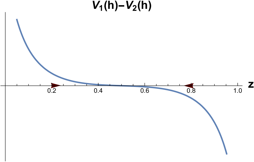
(a) Stable symmetric dispersion: $\phi=0.1$.

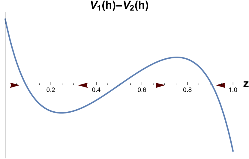
(b) Stable asymmetric dispersion: $\phi=0.3$.

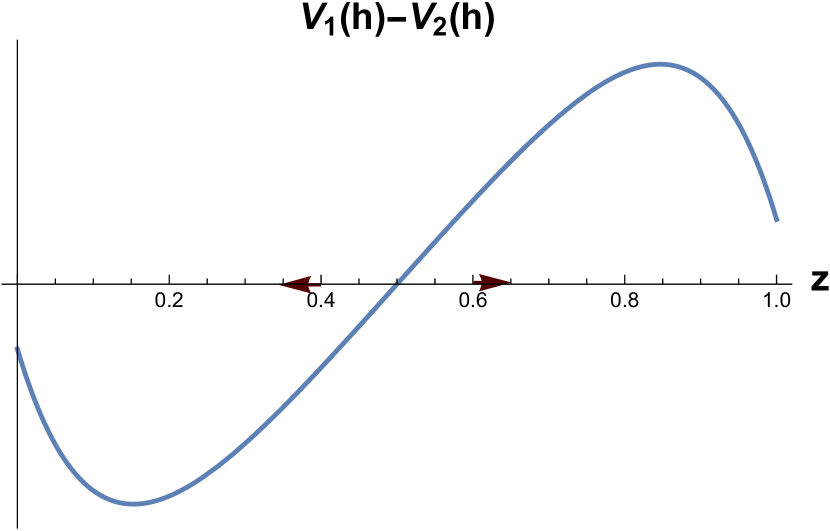
(c) Stable agglomeration: $\phi=0.38$.

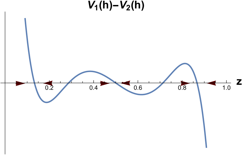
(d) Stable asymmetric dispersion: $\phi=0.4$.

(e) Stable symmetric dispersion: $\phi=0.8$.

Figure 1: Long-run equilibria and their stability as $\phi$ increases.

Figure 10 shows one scenario with five qualitatively different cases, with varying freeness of trade $\phi$, for $b\in[0,\frac{1}{2})$, regarding existence of the model’s long-run spatial distribution, which exhaust all mathematical possibilities for the parameter values $\left(\lambda,\gamma,\phi,\sigma,b\right)=\left(2,0.9,0.4,8,0.339\right)$. As a prelude to the forthcoming Section, Figure 10 also numerically depicts the local stability of each equilibrium, which is to be analysed analytically in greater detail in Section 3.2.

In Figure 1(a), only symmetric dispersion exists and is stable for a very small $\phi$. For a higher trade freeness we have one stable asymmetric dispersion for $z\in\left(\frac{1}{2},1\right]$ as portrayed in Figure 1(b). For a greater $\phi$, Figure 1(c) shows that the asymmetric dispersion equilibrium disappears and symmetric dispersion becomes unstable, whereas agglomeration becomes stable. For an even greater $\phi$, Figure 1(d) illustrates an example of two long-run dispersion equilibria $z^{*}$ for $z\in\left(\frac{1}{2},1\right]$ and symmetric dispersion $z=\frac{1}{2}$, whereby we can observe that both symmetric dispersion and the more agglomerated dispersion equilibrium are locally stable, whereas the less agglomerated equilibrium is unstable. The economy re-disperses and agglomeration does not exist in this particular case. However, as the trade freeness increases further, symmetric dispersion remains stable and all other equilibria disappear. In other words, when $b\in[0,\frac{1}{2})$, the model accounts for a “bubble-shaped” relationship between economic integration and spatial (Pflüger and Südekum,, 2008), whereby firms are initially dispersed, then start to agglomerate in a single region as the trade freeness increases, but then find it worthwhile to relocate to the peripheral regions in order to benefit from higher expected profits due to the sizeable pool of scientists in the core which increases the chance of innovation in the periphery.

The case $b\in(\frac{1}{2},1]$ is much less diversified and can be accounted for resorting to a subset of the pictures from Figure 10. The history as economic integration increases is as follows. For a very low trade freeness, symmetric dispersion is the only stable equilibrium as in Figure 1(a). For an intermediate value of $\phi$, one asymmetric dispersion equilibrium arises which is the only stable one and becomes more asymmetric as $\phi$ increases further. This is akin to the picture in Figure 1(b). Finally, the asymmetric dispersion equilibrium gives rise to stable full agglomeration in one single region once $\phi$ becomes very high. This is illustrated in Figure 1(c).

In other words, when intra-regional interaction is relatively more important ($b>\frac{1}{2}$), the model behaves just like the baseline Pflüger, (2004) model.

In the forthcoming Sections, we will analytically and numerically study in greater detail the local stability of the spatial distributions and the qualitative change in the model’s structure as economic integration increases.

4.2 Stability

4.2.1 Agglomeration

Regarding agglomeration, using (15) in (16), we have that it is stable if:

$$\mathcal{S}\equiv\frac{\gamma\left[(b-1)(\lambda+2)\phi^{2}+2b(\lambda+1)\phi+(b-1)\lambda\right]}{2\sigma\phi}-\frac{\ln\phi}{\sigma-1}>0.$$

The second term is positive. Hence, agglomeration is always stable if the first term is also positive:

$$b>b_{s}\equiv\frac{(\lambda+2)\phi^{2}+\lambda}{(\phi+1)\left[(\lambda+2)\phi+\lambda\right]}.$$

It is easy to check that $b_{s}<\tfrac{1}{2}$ if $\phi\in\left(\frac{\lambda}{\lambda+2},1\right)$, which means that, if $\phi\in\left(\frac{\lambda}{\lambda+2},1\right)$ and $b>\frac{1}{2}$, agglomeration is unstable. In any case, we can conclude that agglomeration is unstable if related variety is too strong.

Let us now define as sustain point (Fujita et al.,, 1999), a value of $\phi$ such that $\mathcal{S}(\phi)=0.$ We have the following result relating the freeness of trade and the relatedness of variety.

Proposition 3.

If $b<\tfrac{1}{2}$, there exist two sustain points, $\phi_{s1}$ and $\phi_{s2},$ and agglomeration is unstable for $\phi\in\left\{\left(0,\phi_{1s}\right)\cup\left(\phi_{2s},1\right)\right\}$ and stable for $\phi\in(\phi_{1s},\phi_{2s})$. If $b>\frac{1}{2}$, there exists a unique sustain point $\phi_{s1}$ and agglomeration is unstable for $\phi\in(0,\phi_{1s})$ and stable if $\phi\in\left(\phi_{1s},1\right)$.

Proof.

See Appendix A. ∎

The result in Proposition 3 suggests that an intermediate level of economic integration favours agglomeration only if the interaction with foreign scientists is relatively more important for the chance of successful innovation. By contrast, if the within region interaction of scientists is more important, agglomeration is only possible when the freeness of trade is high enough.

4.2.2 Symmetric dispersion

Regarding symmetric dispersion $z^{*}=\frac{1}{2}$, using (15) in (16) we can say that it is stable if:

$$\mathcal{B}\equiv\gamma(\sigma-1)\left[2b(\lambda+1)(\phi+1)^{2}-(2\lambda+3)\phi^{2}-2\lambda-1\right]+2\sigma\left(1-\phi^{2}\right)<0.$$ (17)

In fact, it is always unstable if the first term is positive, i.e. if:

$$b>\bar{b}\equiv\frac{(2\lambda+3)\phi^{2}+2\lambda+1}{2(\lambda+1)(\phi+1)^{2}}.$$

This means that if related variety is prohibitively high, symmetric dispersion is surely unstable.

We can observe that $\mathcal{B}$ in (17) is a second degree polynomial in $\phi$ with at most two zeros, i.e., break points $\phi_{b1}$ and $\phi_{b2}$, with $\phi_{b1}<\phi_{b2}$ and has a negative leading coefficient. Therefore if both break points exist, we have that symmetric dispersion is stable for $\phi<\phi_{b1}$, unstable for $\phi\in\left(\phi_{b1},\phi_{b2}\right)$, and stable again for $\phi>\phi_{b2}$. This means that our model accounts for the possibility of initial agglomeration as trade integration increases from a very low level and re-dispersion for very high levels of trade integration.

More specifically, the breakpoints are given by:

$$\phi_{b1} =\frac{\sqrt{\gamma^{2}(\sigma-1)^{2}\left[8b(\lambda+1)^{2}-4\lambda^{2}-8\lambda-3\right]+4\gamma\sigma(\sigma-1)+4\sigma^{2}}-2b\gamma(\lambda+1)(\sigma-1)}{\gamma(\sigma-1)\left[2b(\lambda+1)-2\lambda-3\right]-2\sigma}$$

$$\phi_{b2} =-\frac{\sqrt{\gamma^{2}(\sigma-1)^{2}\left[8b(\lambda+1)^{2}-4\lambda^{2}-8\lambda-3\right]+4\gamma\sigma(\sigma-1)+4\sigma^{2}}+2b\gamma(\lambda+1)(\sigma-1)}{\gamma(\sigma-1)\left[2b(\lambda+1)-2\lambda-3\right]-2\sigma}.$$ (18)

The break point $\phi_{b1}$ lies in the interval $(0,1)$ if and only if:

1. $\gamma\in\left(\dfrac{2\sigma}{(2\lambda+1)(\sigma-1)},1\right)$,

2. $b\in\left[b_{1},b_{2}\right),$

where:

$$b_{1} =\frac{\left[\gamma(2\lambda+1)(\sigma-1)-2\sigma\right]\left[\gamma(2\lambda+3)(\sigma-1)+2\sigma\right]}{8\gamma^{2}(\lambda+1)^{2}(\sigma-1)^{2}},$$

$$b_{2} =\frac{\gamma(2\lambda+1)(\sigma-1)-2\sigma}{2\gamma(\lambda+1)(\sigma-1)}.$$

We have that $b_{1}\in\left(0,\frac{1}{2}\right)$ and $b_{2}\in\left(b_{1},1\right)$. If, additionally, $b<\frac{1}{2}$, then we have also that $\phi_{b2}\in\left(0,1\right)$. This means that the possibility of re-dispersion following agglomeration as $\phi$ increases requires that related variety is neither too high or too low.

However, if $b>\frac{1}{2}$, then $\phi_{b2}$ does not exist and we have a single break point $\phi_{b1}$ if conditions (i) and (ii) are satisfied.

4.2.3 Asymmetric dispersion

Although we cannot find an explicit stability condition for any asymmetric dispersion equilibrium $z^{*}\in\left(\frac{1}{2},1\right)$, we can use equation (23) that solves the equilibrium condition $\Delta v=0$ given implicitly by $\lambda=\lambda^{*}(z)$ in the proof of Proposition 2 (Appendix A.2). Then the stability condition of an asymmetric dispersion equilibrium is given by:

$$\left.\frac{d\Delta v}{dz}(z^{*})\right|_{\lambda=\lambda^{*}(z)}<0.$$

Specifically, using (15) and differentiating (16) with respect to $z$, and evaluating at (23), we get that an assymetric equilibrium $z^{*}\in\left(\frac{1}{2},1\right)$ is stable if $\lambda^{*}(z)>0$ and:

$$\mathcal{G}\equiv (2z-1)\left(\phi^{2}-1\right)\left[(2b-1)\gamma(\sigma-1)(1-2z)^{2}-\sigma\right]+$$

$$+\sigma\left[2z^{2}(\phi-1)^{2}-2z(\phi-1)^{2}+\phi^{2}+1\right]\ln\left[\frac{z(\phi-1)+1}{z(1-\phi)+\phi}\right]<0.$$ (19)

We have the following result.

Proposition 4.

If $b<\frac{1}{2}$ an asymmetric equilibrium $z^{*}\in\left(\frac{1}{2},1\right)$ is stable for a high enough related variety. If $b>\frac{1}{2}$, an asymmetric equilibrium is always stable when it exists.

Proof.

See Appendix A. ∎

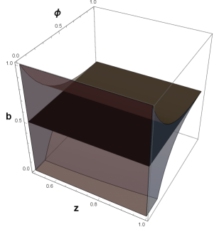
Figure 2: Stability of asymmetric dispersion. The less opaque surface corresponds to $\mathcal{G}<0$ and $\lambda^{*}(z)>0$ in $(z,\phi,b)$–space for $\sigma=8$ and $\gamma=0.9$. The black plane corresponds to $b=\frac{1}{2}.$

Figure 2 illustrates the Proposition by setting $\sigma=8$ and $\gamma=0.9$ and plotting the surface corresponding to $\left\{(z,\phi,b):\mathcal{G}<0\cap\lambda^{*}(z)>0\right\}$. For $b<\frac{1}{2}$, an asymmetric equilibrium may exist that is not stable, and a higher $b$ favours its stability. If $b>\frac{1}{2}$, an asymmetric equilibrium is always stable when it exists, but its existence seems to be favoured by a lower $b$. In other words, an asymmetric equilibrium exists and is stable when $b$ is close enough to $\frac{1}{2}$.

Regarding $\phi$, a higher freeness of trade $\phi$ seems to disfavour the stability of asymmetric dispersion.

5 The impact of economic integration

It is common in geographical economics to study the qualitative change of the spatial economy as economic integration increases. We will now look at some bifurcation diagrams using the freeness of trade, $\phi$, as the bifurcation parameter. To provide a complete gallery, we depict 6 qualitatively different scenarios, keeping most parameter values constant (except for the sixth scenario) and varying $b$, thus placing emphasis on changes in the value of the weight of within-region interaction. Two additional illustrations for different parameter values are provided in Appendix B. The illustrations, 8 in total, exhaust all mathematical/numerical possibilities. The six scenarios analysed in this Section are as follows:

1. $\left(\lambda,\gamma,\sigma,b\right)=\left(2,0.9,8,0.33\right)$;

2. $\left(\lambda,\gamma,\sigma,b\right)=\left(2,0.9,8,0.338\right)$;

3. $\left(\lambda,\gamma,\sigma,b\right)=\left(2,0.9,8,0.339\right)$;

4. $\left(\lambda,\gamma,\sigma,b\right)=\left(2,0.9,8,0.35\right)$;

5. $\left(\lambda,\gamma,\sigma,b\right)=\left(2,0.9,8,0.55\right)$;

6. $\left(\lambda,\gamma,\sigma,b\right)=\left(4,0.9,8,0.55\right)$;

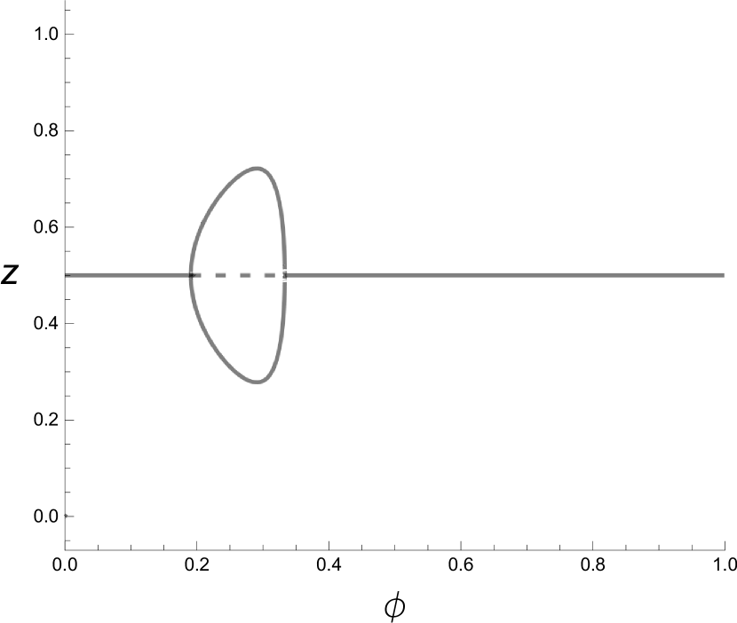
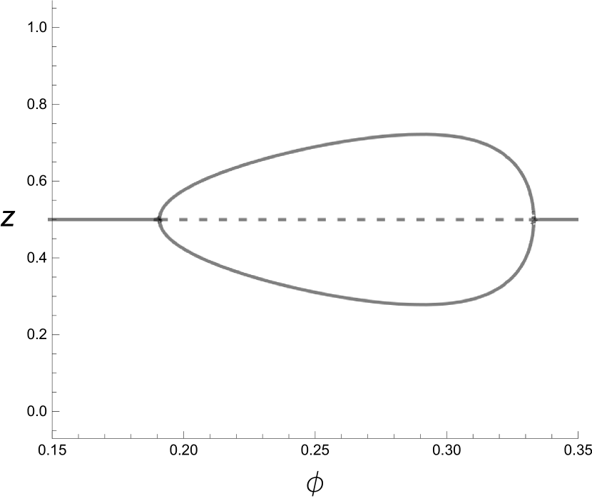
Figure 3: Bifurcation diagram for scenario (i). Filled lines correspond to stable equilbria and dashed lines correspond to unstable equilibria.

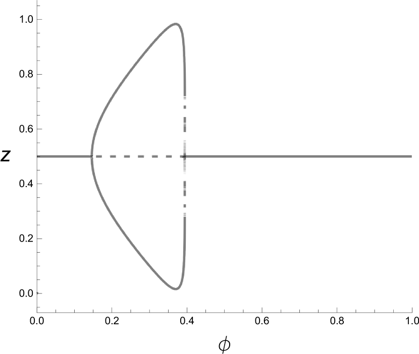
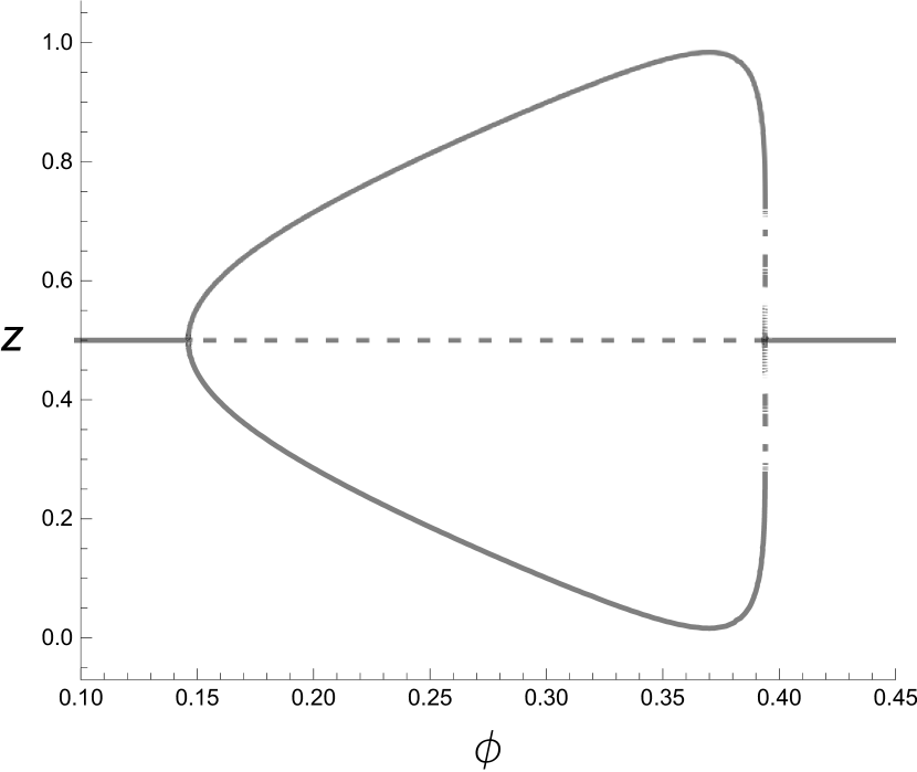
Figure 4: Bifurcation diagram for scenario (ii). Filled lines correspond to stable equilbria and dashed lines correspond to unstable equilibria.

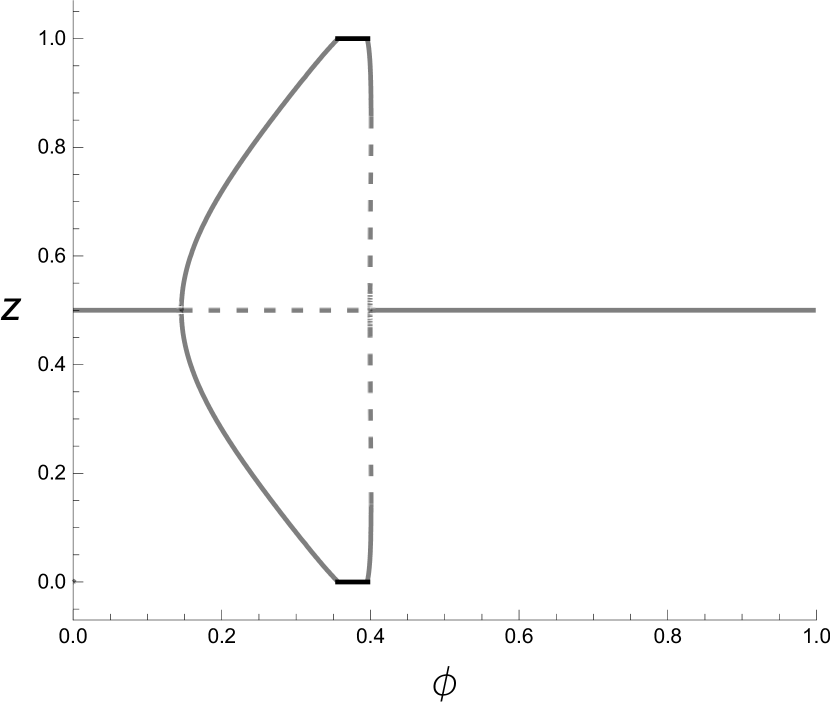
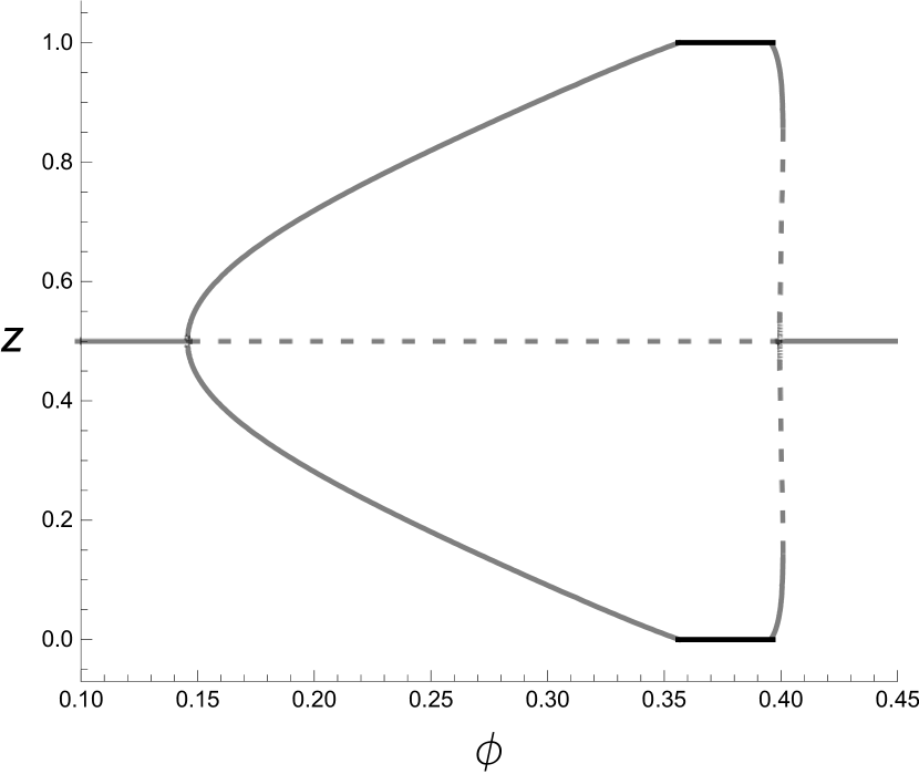
Figure 5: Bifurcation diagram for scenario (iii). Filled lines correspond to stable equilbria and dashed lines correspond to unstable equilibria.

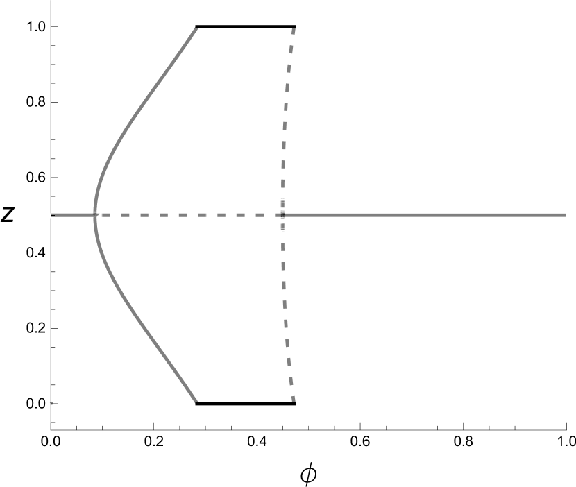
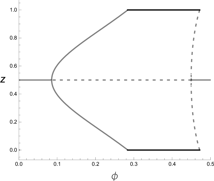
Figure 6: Bifurcation diagram for scenario (iv). Filled lines correspond to stable equilbria and dashed lines correspond to unstable equilibria.

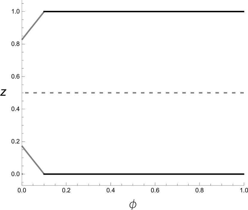
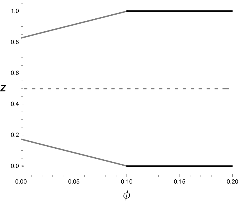
Figure 7: Bifurcation diagram for scenario (v). Filled lines correspond to stable equilbria and dashed lines correspond to unstable equilibria.

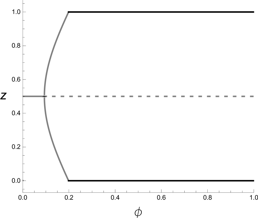
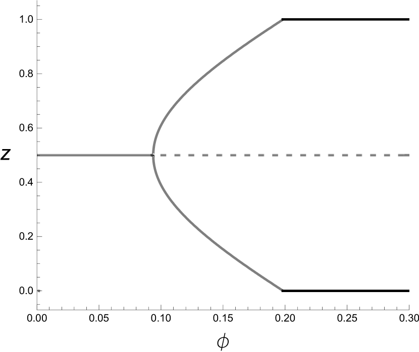
Figure 8: Bifurcation diagram for $(\lambda,\gamma,\sigma,b)=(4,0.9,8,0.55)$. Filled lines correspond to stable equilbria and dashed lines correspond to unstable equilibria.

For a prohibitively low related variety, scientists disperse evenly among the two regions, irrespective of the value of the freeness of trade. The economic intuition is simple: a lower $b$ implies higher chance of successful innovation with more scientists living in the other region. Hence, the nominal wage is higher when the scientists are more evenly distributed.

In scenario (i), shown in Figure 3, related variety is such that within-region interaction is relatively more important ($b=0.33$) but is still low. For a low freeness of trade, symmetric dispersion is stable because firms wish to avoid the burden of a very costly transportation supplying to farmers from full agglomeration in a single region. As $\phi$ increases, the economy initially agglomerates, but then re-disperses as $\phi$ increases further. This re-dispersion process occurs because, for a very high economic integration, firms find it profitable to relocate to the less industrialized region in order to benefit from the pool of scientists in the more agglomerated region, which generates a higher chance of innovation and thus higher expected profits. Noteworthy, the turning point in the agglomeration process happens before industry reaches full agglomeration in a single region, as in Pflüger and Südekum, (2008). However, contrary to the latter, our model does not predict full agglomeration in the entire parameter range of economic integration when related variety is low enough.

Re-dispersion in scenario (i) is more akin to geographical economic models of vertical linkages between upstream and downstream firms by Krugman and Venables, (1995); Venables, (1996) and Puga, (1999). However, in these models, re-dispersion is smooth altogether and occurs when workers are inter-regionally immobile and firms become too sensitive to regional cost differentials when economic integration is very high.

In scenario (ii), illustrated by Figure 4, related variety is just slightly higher, and the model still accommodates for re-dispersion. However, the re-dispersion process is not smooth – the economy suddenly jumps to symmetric dispersion from a fairly asymmetric equilibrium spatial distribution.

Scenario (iii) also just slightly increases related variety compared to the previous scenario (see Figure 5), and the story of spatial outcomes as economic integration increases is very similar, except that, in this case, full agglomeration is stable for a small range of intermediate values of $\phi$, as predicted by Proposition 3. The parametrization here also corresponds to that illustrated in Figure 10.

The re-dispersion processes of scenarios (ii) and (iii) are uncommon in the literature of geographical economics; rather, such jumps occur in early models (Fujita et al.,, 1999; Baldwin et al.,, 2003) from the state of symmetric dispersion to catastrophic agglomeration (Behrens and Robert-Nicoud,, 2011). The reverse discontinuous jump, i.e., from symmetric dispersion to partial agglomeration as trade costs steadily decrease, has been uncovered in the model by Pflüger and Tabuchi, (2010), where all production factors, except land, which is used both for housing and production, are inter-regionally mobile. Their conclusions about spatial outcomes reveal a line-symmetry of scenario (iii): as integration increases, the economy jumps discontinuously from symmetric dispersion to partial agglomeration, and the ensuing re-dispersion is gradual and continuous.

Figure 6 illustrates scenario (iv) and shows that the sudden re-dispersion process under a slightly higher $b$ now happens from the state of full agglomeration directly to the state of symmetric dispersion. In both scenarios (iii) and (iv), the state of agglomeration is stable for intermediate values of economic integration, as in Robert-Nicoud, (2008).

In scenario (v), for a sufficiently high $b>1/2$, within-region interaction among scientists improves the chances of innovation enough such that the real wage becomes higher when they are either partially agglomerated in one region for low values of $\phi$, or completely agglomerated in one region for a high enough $\phi$. This is portrayed in Figure 7. Scenario (v) precludes the so-called “no black-hole condition” (Fujita et al.,, 1999), a condition that the constant elasticity of substitution $\sigma$ must be high enough such that symmetric dispersion can be stable for low enough economic integration. As argued by Gaspar et al., (2018), this condition may be unwarranted if its exclusion allows for spatial outcomes other than ubiquitous agglomeration.

We can thus conclude that a higher related-variety is associated with a more pronounced agglomeration during the industrialization process, for intermediate values of economic integration, until eventually it becomes so high that re-dispersion is no longer possible because within-region interaction among scientists is too important to make any deviation to a deindustrialized region worthwhile.

In scenario (vi) we illustrate the qualitative change in the spatial structure of the economy as $\phi$ increases for $b>1/2$, but with a higher $\lambda$, since, with the parameter values of the previous scenario, agglomeration would be ubiquitously stable (and hence uninteresting) for higher values of $b$. In Figure 8, we can observe the typical supercritical pitchfork that we can observe in the original Pflüger, (2004) model. That is, for low levels of economic integration, symmetric dispersion is stable. As $\phi$ increases, one region smoothly becomes more and more industrialized en route to a full agglomeration whereby that region becomes a core.

Noteworthy, in any scenario for which a break point exists at symmetric dispersion, it can be shown analytically that the model undergoes a pitchfork bifurcation, either supercritical or subcritical, depending on the parameter values). Additionally, in Figures 4 and 4 (scenarios (ii) and (iii)), a limit point $\phi\equiv\phi_{l}\in(\phi_{b2},1)$ is discernible at which two asymmetric equilibria, along a curve tangent to $\phi_{l}$ that lies to its left, collide and coalesce. This suggests that in both scenarios (i) and (ii) the model undergoes a saddle-node bifurcation at some asymmetric equilibrium $z^{*}\in\left(\frac{1}{2},1\right)$. This kind of bifurcation also appears in the two-region footloose entrepreneur model by Forslid and Ottaviano, (2003) with heterogeneous agents analysed by Castro et al., (2021) and also in the Pflüger, (2004) model extended to multiple regions by Gaspar et al., (2018). This kind of bifurcation seems to be associated with discontinuous jumps between some asymmetric equilibrium other than agglomeration and the symmetric dispersion once $\phi$ rises (falls) above (below) some threshold level.

In Appendix B we change the benchmark parameter values and further illustrate how changes in $b$ can bring about richer implications regarding the qualitative structure of the spatial economy.

6 On the role of regional interaction

It is worthwhile investigating how different types of regional interaction determining the success of innovation affect the spatial outcomes in the economy. The process of (de)industrialization as economic integration increases can be shown to vary quite a lot under different functional forms for the probability of a successful innovation.

6.1 A simple scenario

We first consider a slight modification in the success of innovation that deems the model even more simple, but leads to very different results regarding the relationship between regional interaction in the production of knowledge and the long-run equilibrium spatial outcomes.

Suppose now that a firm producing variety $s$ at region $i$ reaches a leading quality grade $k$ with probability:

$$\Phi_{i}^{S}(s)=\min\left\{\dfrac{z_{i}+cz_{j}}{a_{i}(s)}\gamma A,1\right\},$$ (20)

where $c\in(0,1)$ now represents the weight of inter-regional interaction in the chance of successful innovation. In other words, it is a measure of unrelated variety. We assume a parametrization that guarantees that the first term lies in the interval $[0,1]$.

This specification yields at most one asymmetric equilibrium $z^{*}\in\left(\frac{1}{2},1\right]$ (see Appendix C.1), besides the symmetric dispersion which remains an invariant pattern. Agglomeration exists and is stable for a high enough freeness of trade (sustain point $\phi_{s}^{S}$ and symmetric dispersion is stable for a low enough freeness of trade (break point $\phi_{b1}^{S}$ (see Appendix C.2). Moreover, it is possible to show that the model undergoes a supercritical pitchfork bifurcation at the symmetric dispersion (C.3), just as in Pflüger, (2004).

Consider an increase in the parameter $c$. We have:

$$\frac{\partial\Delta v^{S}}{\partial c}=\frac{\gamma\mu(2z-1)\left[\lambda-2z^{2}+\phi^{2}(\lambda+2(z-1)z+2)+2z\right]}{2\sigma\left[z(\phi-1)+1\right]\left[z(\phi-1)-\phi\right]},$$

which is negative for $z\in\left(\frac{1}{2},1\right)$. In other words, a higher $c$ decreases the utility differential. Castro et al., (2021) have recently demonstrated that an exogenous shock in any parameter that leads to a higher utility differential favours agglomeration and discourages dispersion. We have the following result.

Lemma 1.

Under $\Phi_{i}^{S}(s)$, an increase in the weight of inter-regional interaction in the chance of innovation (i.e. higher $c$) does not favour agglomeration.

Proof.

See Proposition 9 of (Castro et al.,, 2021, p.197). ∎

In other words, a higher $c$ favours symmetric dispersion and discourages agglomeration. As illustrated in Figure 9, a higher $c$ shifts the pitchfork bifurcation rightwards.

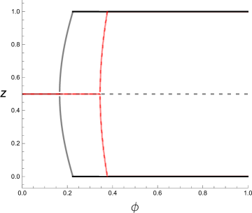
Figure 9: Bifurcation diagrams: (i) to the left, in black, we set $c=0.7$; (ii) to the right, in red, we set $c=0.9$. Parameter values are $(\sigma,\gamma,\lambda)=(8,1,4).$

The interpretation behind these results is very straightforward: a higher $c$ implies higher chance of successful innovation with more scientists living in the other region. Hence, the nominal wage is higher when the scientists are more evenly distributed. So, a higher $c$ makes stability of symmetric dispersion (agglomeration) more (less) likely for a higher range of $\phi$, and asymmetric dispersion becomes stable for a higher freeness of trade.

In sum, under this second specification with $\Phi_{i}^{S}(s)$ in (20), agglomeration is a smooth and progressive progress as the trade freeness increases, and the unrelatedness of variety measured by $c$ adds an additional dispersion force to the benchmark model. The most striking contrast with the first scenario is the absence of a “bubble” shaped relation between economic integration and spatial imbalances in the second scenario.

6.2 Multiplicative case: a numerical analysis

Several other functional forms for $\Phi_{i}(s)$ could be worth checking. In fact, it is worth considering the case where scientists are imperfect substitutes from a firm’s innovative perspective. For instance, a Cobb-Douglas specification such as:

$$\Phi_{i}^{CD}(s)=\min\left\{\dfrac{z_{i}^{b}z_{j}^{1-b}}{a_{i}(s)}\gamma A,1\right\},$$ (21)

yields a multiplicative scenario, and thus brings our setup closer to Berliant and Fujita, (2008). Again we shall impose a parametrization that guarantees that the first term lies in the interval $[0,1]$.

Regarding agglomeration, it cannot be an equilibrium because $\Delta v(1)=\frac{\mu\ln\phi}{\sigma-1}<0$. Since no innovation occurs, expected profits are driven down to zero and the only thing that matters is the cost-of-living, which is positive in the fully agglomerated region. However, if an agent moves to the “empty” region, innovation occurs through inter-regional interaction and he will earn a positive nominal wage, which means that exogenous perturbations always increase the utility of agents. While this may strike as an implausible outcome, one way to counter this would be to specify a different probability for corner equilibria, potentially following Berliant and Fujita, (2008).

The symmetric dispersion can be shown to retain the qualitative properties of the benchmark case analyzed in Section 3.2.2. That is, there exist two break points $\phi_{b1}$ and $\phi_{b2}$ given by (18) and symmetric dispersion is stable for $\phi\in\left\{(0,\phi_{b1})\cup(\phi_{b2},1)\right\}$, and unstable for $\phi\in\left(\phi_{b1},\phi_{b2}\right)$.

We can grasp the general qualitative behaviour and properties of the model under $\Phi_{i}^{CD}(s)$ by depicting a gallery of bifurcation diagrams for several different values of $b$.The benchmark parameter values are $(\sigma,\gamma,\lambda)=(8,1,4)$, while the value for $b$ is reported in the caption of each picture.

(a) Stable symmetric dispersion: $b=0.1$.

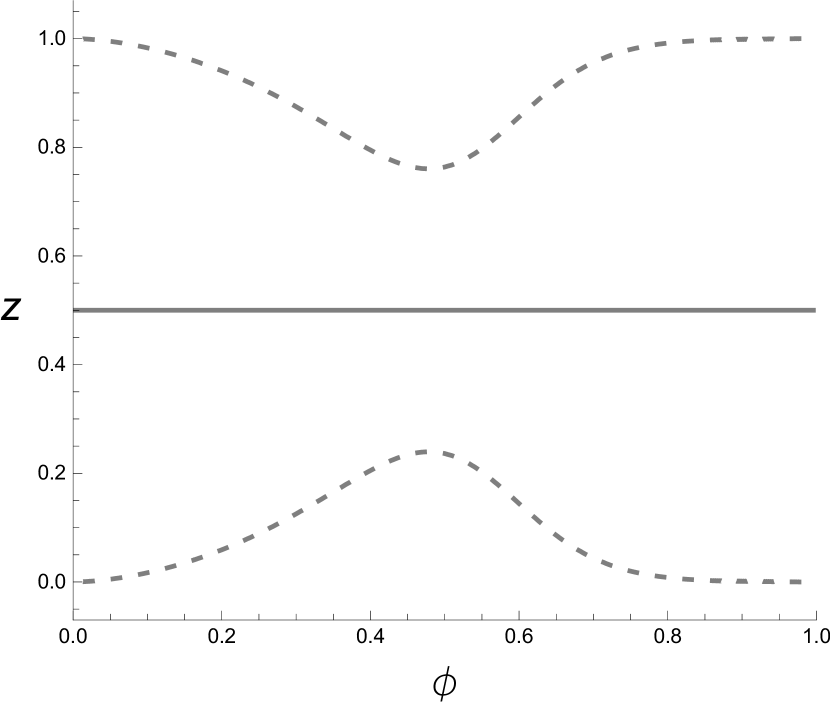
(b) Stable symmetric dispersion: $b=0.44$.

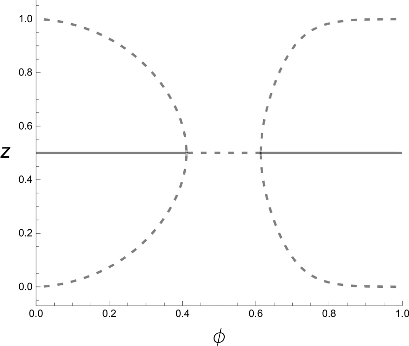
(c) Stable symmetric dispersion for $\phi<\phi_{b1}$ and $\phi>\phi_{b2}$: $b=0.45$.

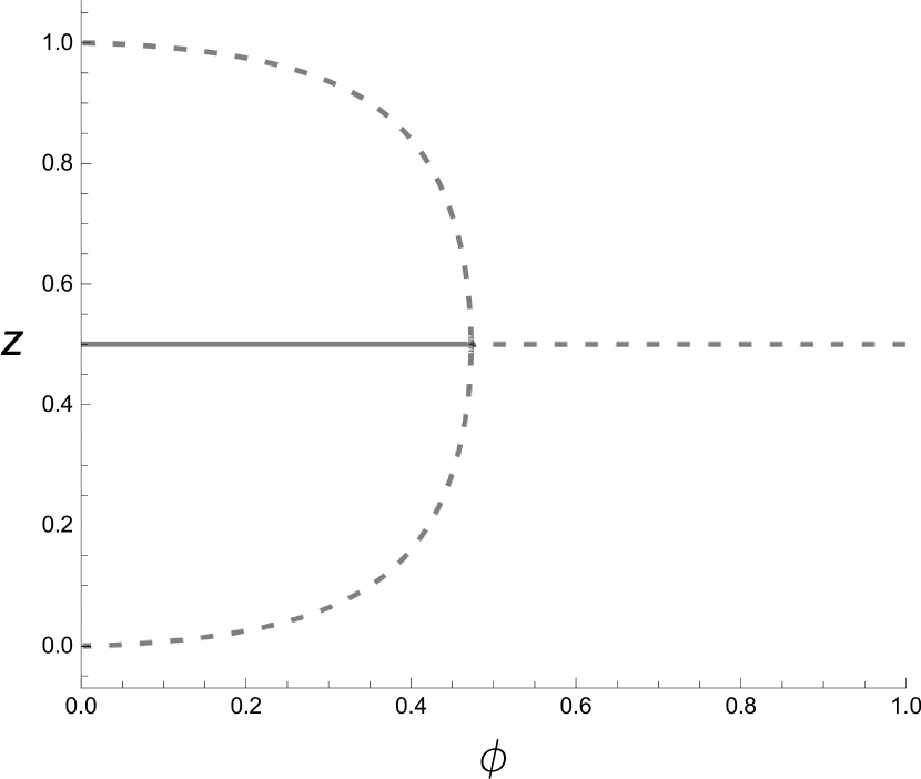
(d) Stable symmetric dispersion for $\phi<\phi_{b1}$: $b=0.5$.

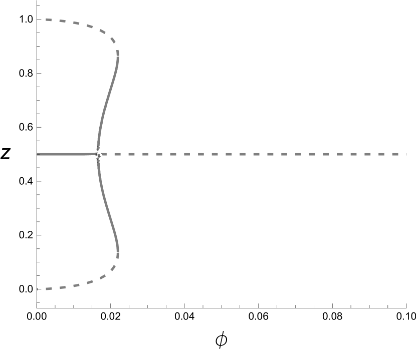
(e) Stable symmetric dispersion for $\phi<\phi_{b1}$ and stable asymmetric dispersion for $\phi>\phi_{b1}$: $b=0.65$.

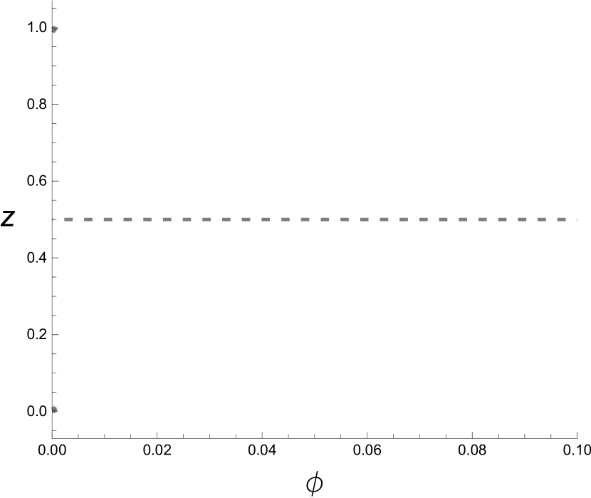
(f)
No stable equilibria: $b=0.75$

.

Figure 10: Bifurcation diagram for $(\lambda,\gamma,\sigma,b)=(4,1,8)$. Filled lines correspond to stable equilibria and dashed lines correspond to unstable equilibria.

As $b$ increases from a very small value, initially only symmetric dispersion exists and is stable (Figure 10(a)). Eventually there emerge two curves of unstable asymmetric dispersion equilibria (Figure 10(b)), one with a minimum and the other with a maximum (for the same $\phi$ due to symmetry. For higher levels of $b$, the extrema collide vertically at symmetric dispersion and two curves of asymmetric dispersion equilibria branch from two break points. Symmetric dispersion is stable below the lowest break point and above the highest break point, and unstable in between (Figure 10(c)). Further increases in $b$ will make the highest breakpoint disappear and we end up with a subcritical pitchfork bifurcation (Figure 10(d)), as in Fujita et al., (1999), whereby symmetric dispersion is stable for low values of $\phi$ and becomes unstable for high values of $\phi$. The main difference is that there are no stable equilibria above the break point. If $b$ increases even more, we end up with a supercritical pitchfork bifurcation whereby a stable symmetric dispersion loses stability for $\phi$ large enough (Figure 10(e)). This state encounters a primary branch of stable asymmetric equilibria that, apparently, undergoes a secondary saddle-node bifurcation. Finally, for a prohibitively high value of $b$, there are no stable equilibria in the model, as shown by Figure 10(f).

This scenario with $\Phi_{i}^{CD}(s)$ as the chance of a successful innovation departs from the previous two cases in two major aspects. First, it reverses the predictions about the spatial distribution of economic activities with respect to increases in $\phi$ (except for the case in Figure 10(c) where re-dispersion is possible). While this may be hard to explain from an economic point of view, one may conjecture that this may be due to the multiplicative nature of the probability of innovation in this scenario that contrasts with the additive nature in the first benchmark case and in the simpler case of $\Phi_{i}^{S}(s)$. Second, the last scenario seems to be poorer in terms of predictions since, e.g., the only stable asymmetric equilibria exist for a very small range and values of $\phi$.

7 Concluding remarks

In this paper we have analysed a two-region model with vertical innovations that enhance the quality of varieties of the horizontally differentiated manufactures produced in each of the two regions. We looked at how the creation and diffusion of knowledge and increasing returns in manufacturing interact to shape the spatial economy. Innovations occur with a probability that depends on the inter-regional interaction between researchers (mobile workers).

We find that, if the weight of interaction with foreign scientists is relatively more important for the success of innovation, the model accounts for re-dispersion of economic activities after an initial stage of progressive agglomeration as transport costs decrease from a high level. However, the relationship between economic integration and spatial imbalances is far from trivial, as we have shown a myriad of different qualitative possibilities that depend on the weight of intra-regional interaction between scientists, i.e. on the level of related variety (Frenken et al.,, 2007). We show that the re-dispersion process is only smooth (Fujita and Thisse,, 2013) when interaction with foreign cultures is relatively more important, which happens for a low enough related variety. If related variety is intermediate, there is a discontinuous jump towards symmetric dispersion from either full agglomeration or partial agglomeration. If related variety is too high, re-dispersion is precluded and full agglomeration is the only stable outcome for high enough economic integration, as in most early NEG models (Fujita et al.,, 1999; Baldwin et al.,, 2003; Pflüger,, 2004).

Our main results so far may seem to hinge on the functional form for the probability of innovating. We have studied two simple different additive cases and provided insights on a multiplicative scenario. The additive cases are useful not only for tractability but also capture the idea that public knowledge transfers imperfectly across space, as argued by Krugman, 1991a , Bond-Smith, (2021) and supported by the empirical evidence of the seminal paper by Audretsch and Feldman, (1996). However, it could be worthwhile further investigating how different types of regional interaction determining the success of innovation affect the spatial outcomes in the economy. The process of (de)industrialization as economic integration increases can be shown to vary quite a lot under different functional forms for the probability of a successful innovation. This becomes noteworthy when we take the simplest case of knowledge creation depending on scientists across different regions, and even more so when knowledge creation is of multiplicative nature as in e.g. Berliant and Fujita, (2012).

Appendix A Proofs

This appendix contains the more cumbersome formal proofs that support our main results.

A.1 Proof of proposition 1

Differentiating $\Delta v(z)$ in (16) yields:

$$\frac{d\Delta v}{dz}(z)=\frac{\mu P(z)}{2(\sigma-1)\sigma\left[z(\phi-1)+1\right]{}^{2}\left[z(1-\phi)+\phi\right]{}^{2}},$$ (22)

where:

$$P(z)=a_{1}z^{4}+a_{2}bz^{3}-2(1-\phi)a_{3}z^{2}+2(1-\phi)a_{4}z+a_{5},$$

with:

$$a_{1}= 4(1-2b)\gamma\mu(\sigma-1)(\phi-1)^{3}(\phi+1)$$

$$a_{2}= 8(2b-1)\gamma\mu(\sigma-1)(\phi-1)^{3}(\phi+1)$$

$$a_{3}= \gamma(\sigma-1)\left\{b(\phi+1)\left[(\lambda-2)\phi^{2}-\lambda+18\phi-4\right]-\phi\left[\lambda(\phi-1)\phi+\lambda+6\phi\right]+\lambda-8\phi+2\right\}$$

$$+\sigma(\phi+1)(\phi-1)^{2}$$

$$a_{4}= \gamma(\sigma-1)\left\{\lambda(\phi-1)\left[b(\phi+1)^{2}-\phi^{2}-1\right]+2\phi\left[b(\phi+1)(\phi+5)-\phi(\phi+2)-3\right]\right\}$$

$$+\sigma(\phi+1)(\phi-1)^{2}$$

$$a_{5}= \gamma(\sigma-1)\left\{\lambda\left(\phi^{2}+1\right)\left[b(\phi+1)^{2}-\phi^{2}-1\right]+2\phi\left[b\left(\phi^{3}+3\phi^{2}+\phi-1\right)-\phi\left(\phi^{2}+\phi+1\right)+1\right]\right\}$$

$$-2\sigma\phi\left(\phi^{2}-1\right).$$

The denominator of (22) is positive, which means that the sign of $\frac{d\Delta v}{dz}(z)$ is given by the sign of $P(z)$, which is a fourth degree polynomial in $z$. Therefore, $\Delta v(z)$ has at most four turning points and, thus, at most five equilibria for $z\in[0,1]$. We know that $z=\frac{1}{2}$ is an invariant pattern. By symmetry, we can establish that there exist at most two equilibria for $z>\tfrac{1}{2}$, which concludes the proof. $\square$

A.2 Proof of Proposition 2

Proceeding in a familiar fashion as in Gaspar et al., (2018, 2021), the equilibrium condition $\Delta v(z)=0$ yields:

$$\lambda\equiv\lambda^{*}(z)=-2\frac{b_{1}b_{2}+b_{3}\ln\left[\frac{z(\phi-1)+1}{z(1-\phi)+\phi)}\right]}{b_{4}},$$ (23)

where:

$$b_{1} =\gamma(\sigma-1)(2z-1)$$

$$b_{2} =\phi^{2}\left[2b(z-1)z+b-z^{2}+z-1\right]+(1-2b)(z-1)z+b\phi$$

$$b_{3} =\sigma\left[z(\phi-1)+1\right]\left[z(\phi-1)-\phi\right]$$

$$b_{4} =\gamma(\sigma-1)(2z-1)\left[b(\phi+1)^{2}-\phi^{2}-1\right].$$

It is easy to note that $\lambda^{*}(z)$ has a vertical asymptote if and only if $b_{4}=0$, i.e., iff:

$$b=\hat{b}\equiv\frac{\phi^{2}+1}{(\phi+1)^{2}}.$$

For $z\in\left(\frac{1}{2},1\right],$ the log term of $\lambda^{*}(z)$ is negative, as is $b_{3}$. Next, we have $b_{1}>0$, and $b_{2}>0$ if:

$$b\geq\underline{b}\equiv\frac{(z-1)z\left(\phi^{2}-1\right)+\phi^{2}}{2(z-1)z\left(\phi^{2}-1\right)+\phi(\phi+1)},$$

where $0<\underline{b}<\hat{b}$. Since $b_{4}<0$ only if $b<\hat{b}$, we have that $\lambda^{*}(z)>0$ if $b\in\left[\underline{b},\hat{b}\right)$ and $\lambda^{*}(z)<0$ if $b\in\left(\hat{b},1\right)$. For $b\in\left(0,\underline{b}\right)$, we need further inspection.

We have that:

$$\frac{\partial\lambda^{*}}{\partial b}(z)=\frac{2(\phi+1)\left[z(\phi-1)+1\right]\left[z(\phi-1)-\phi\right]\left\{\gamma(\sigma-1)(2z-1)(\phi-1)+\sigma(\phi+1)\ln\left[\frac{z(\phi-1)+1}{z(1-\phi)+\phi)}\right]\right\}}{\gamma(\sigma-1)(2z-1)\left[-b(\phi+1)^{2}+\phi^{2}+1\right]^{2}},$$

which is positive for all $z\in\left(\frac{1}{2},1\right].$ The unique zero of $\lambda^{*}(z)$ in terms of $b$ is given by:

$$b=\tilde{b}\equiv\frac{\gamma(\sigma-1)(2z-1)\left[(z-1)z\left(\phi^{2}-1\right)+\phi^{2}\right]-\sigma\left[z(\phi-1)+1\right]\left[z(\phi-1)-\phi\right]\ln\left[\frac{z(\phi-1)+1}{z(1-\phi)+\phi)}\right]}{\gamma(\sigma-1)(2z-1)(\phi+1)\left[2(z-1)z(\phi-1)+\phi\right]},$$

with $\tilde{b}<\underline{b}$ and $\lambda^{*}(z)>0$ for $b\in(\tilde{b},\hat{b})$. It is possible to show that $\tilde{b}$ is increasing in $\gamma.$ Moreover, we have $\tilde{b}=0$ if and only if:

$$\gamma=\gamma_{c}\equiv\frac{\sigma\left[z(1-\phi)-1\right]\left[z(1-\phi)+\phi\right]\ln\left[\frac{z(\phi-1)+1}{z(1-\phi)+\phi}\right]}{(\sigma-1)(2z-1)\left[(z-1)z\left(\phi^{2}-1\right)+\phi^{2}\right]}>0.$$

This means that $\tilde{b}\geq 0$ if $\gamma\geq\gamma_{c}$ and $\tilde{b}<0$ if $\gamma<\gamma_{c}$ and $\gamma_{c}\in(0,1]$. Since $\gamma_{c}\in(0,+\infty)$, we have $\tilde{b}<0$ if $\gamma_{c}>1$. As a result, we have $\tilde{b}<0$ if $\gamma\in\left(0,\min\{1,\gamma_{c}\}\right)$ and $\tilde{b}\geq 0$ if $\gamma\in\left[\min\{1,\gamma_{c}\},1\right)$. Then $\lambda^{*}(z)>0$ if $\gamma\in\left(0,\min\{1,\gamma_{c}\}\right)$ and $b\in(0,\hat{b})$. Otherwise, we have $\lambda^{*}(z)>0$ if $\gamma\in\left[\min\{1,\gamma_{c}\},1\right)$ and $b\in(\tilde{b},\hat{b}).$ Therefore, $\lambda^{*}(z)$ is positive for $b\in\left(\max\left\{0,\tilde{b}\right\},\hat{b}\right)$ and negative for $b\in\left\{\left(0,\max\left\{0,\tilde{b}\right\}\right)\cup\left(\hat{b},1\right)\right\}$, where $\max\left\{0,\tilde{b}\right\}$ depends on $\gamma_{c}$ and on the value of $\gamma$ as described above.

Thus, we can assert that, if $b\in\left(\max\left\{0,\tilde{b}\right\},\hat{b}\right)$, there exists a value of $\lambda>0$ such that at least one (at most two) dispersion equilibrium $z\equiv z^{*}\in\left(\frac{1}{2},1\right]$ exists. This concludes the proof. $\square$

A.3 Proof of Proposition 3

We have:

$$\lim_{\phi\rightarrow 0^{+}}\mathcal{S}(\phi)=-\infty\text{ and }\text{$\mathcal{S}(1)=\frac{\gamma(2b-1)(\lambda+1)}{\sigma}.$}$$

Therefore, $S(1)>0$ if $b>\tfrac{1}{2}$ and we conclude that $\mathcal{S}(\phi)$ has at least one zero for $\phi\in\left(0,1\right)$. Further, we have:

$$\dfrac{d\mathcal{S}}{d\phi}(\phi)=\dfrac{1}{2\phi^{2}}\left\{\frac{\gamma(b-1)\left[\lambda\left(\phi^{2}-1\right)+2\phi^{2}\right]}{\sigma}-\frac{2\phi}{\sigma-1}\right\},$$

whose sign depends on that of the second term, which is a second degree polynomial and thus has at most two zeros $\left\{\phi^{-},\phi^{+}\right\}$, with $\phi^{+}>\phi^{-}$. However, only $\phi^{+}$ lies on the interval $\phi\in\left(0,1\right)$:

$$\phi^{+}=\frac{\sigma\left[\frac{1}{\sigma-1}-\sqrt{\frac{\gamma^{2}(b-1)^{2}\lambda(\lambda+2)}{\sigma^{2}}+\frac{1}{(\sigma-1)^{2}}}\right]}{\gamma(b-1)(\lambda+2)}.$$

Given that the leading coefficient of the polynomial is negative, we have that $\mathcal{S}(\phi)$ is increasing for $\phi\in\left(0,\phi^{+}\right)$ and decreasing for $\phi\in\left(\phi^{+},1\right)$. Thus, $\mathcal{S}(\phi)$ has at most two zeros for $\phi\in\left(0,1\right)$, called sustain points $\phi_{s1}$ and $\phi_{s2}$ (with $\phi_{s1}<\phi_{s2}$). If $b<\tfrac{1}{2}$, there exist two sustain points $\phi_{s1}\in\left(0,1\right)$ and $\phi_{s2}\in\left(0,1\right)$ and we have $\mathcal{S}(\phi)<0$ for $\phi\in\left\{\left(0,\phi_{1s}\right)\cup\left(\phi_{2s},1\right)\right\}$ and $\mathcal{S}(\phi)>0$ for $\phi\in(\phi_{1s},\phi_{2s})$. If $b>\tfrac{1}{2}$, there exists one unique sustain point $\phi_{s1}\in\left(0,1\right)$ and we have $\mathcal{S}(\phi)<0$ for $\phi\in\left(0,\phi_{1s}\right)$ and $\mathcal{S}(\phi)>0$ for $\phi\in\left(\phi_{1s},1\right)$, which concludes the proof. $\square$

A.4 Proof of Proposition 4

Taking the derivative of $\mathcal{G}$ in (19) with respect to $b$ we get:

$$\frac{\partial\mathcal{G}}{\partial b}=-2\gamma(\sigma-1)(2z-1)^{3}\left(1-\phi^{2}\right)<0,\ \ z\in\left(\frac{1}{2},1\right)$$

Next, solving $\mathcal{G}$ in (19) for $b$ yields:

$$b=b_{c}\equiv\frac{(2z-1)\left(1-\phi^{2}\right)\left[\sigma+\gamma(\sigma-1)(1-2z)^{2}\right]-\sigma\left[2z^{2}(\phi-1)^{2}-2z(\phi-1)^{2}+\phi^{2}+1\right]\ln\left[\frac{z(\phi-1)+1}{z(1-\phi)+\phi}\right]}{2\gamma(\sigma-1)(2z-1)^{3}\left(1-\phi^{2}\right)}.$$ (24)

As a result, we have $\mathcal{G}>0$ for $b<b_{c}$ and $\mathcal{G}<0$ for $b>b_{c}$. Next, we will prove that $b_{c}<1/2$.

First, notice that $\lim_{\phi\rightarrow 1}b_{c}=\frac{1}{2}.$ Next, we have:

$$\dfrac{\partial b_{c}}{\partial\phi}=\frac{\sigma\mathcal{N}}{2\gamma(\sigma-1)(2z-1)^{3}\left(\phi^{2}-1\right)^{2}\left[z(\phi-1)+1\right]\left[z(\phi-1)-\phi\right]},$$

where:

$$\mathcal{N}= (2z-1)\left(\phi^{2}-1\right)\left[2z^{2}(\phi-1)^{2}-2z(\phi-1)^{2}+\phi^{2}+1\right]-$$

$$-4\left[z(\phi-1)+1\right]{}^{2}\left[z(1-\phi)+\phi\right]{}^{2}\ln\left[\frac{z(\phi-1)+1}{z(1-\phi)+\phi}\right].$$

The numerator of the derivative is negative. As for $\mathcal{N}$, observe that:

$$\dfrac{\partial\mathcal{N}}{\partial z}= -4\sigma(2z-1)(\phi-1)^{2}\times$$

$$\times\left\{(2z-1)\left(1-\phi^{2}\right)+2\left[z(\phi-1)+1\right]\left[z(\phi-1)-\phi\right]\ln\left[\frac{z(\phi-1)+1}{z(1-\phi)+\phi}\right]\right\}.$$

The first term inside the curly brackets is positive and the second one is negative as is the log term. Therefore, we have $\frac{\partial\mathcal{N}}{\partial z}<0$. Since $\mathcal{N}\left(z=\frac{1}{2}\right)=0$ and given that $\mathcal{N}$ is continuous in $z$, we can conclude that $\mathcal{N}<0$ for $z\in\left(\frac{1}{2},1\right)$. Thus, we have $\frac{\partial b_{c}}{\partial\phi}>0,$ which means that $b_{c}<\frac{1}{2}$. Thus, if $b>\frac{1}{2}$, we have $\mathcal{G}<0$ for any value of $\lambda$ such that $\lambda^{*}(z)>0$. This concludes the proof.

Appendix B Related variety and economic integration: additional illustrations

In this Appendix we change the benchmark parameter values to find out whether the value of $b$ can bear more drastic implications to the qualitative structure of the spatial economy. Particularly, we set $(\lambda,\gamma,\sigma)=(1,0.9,8)$.

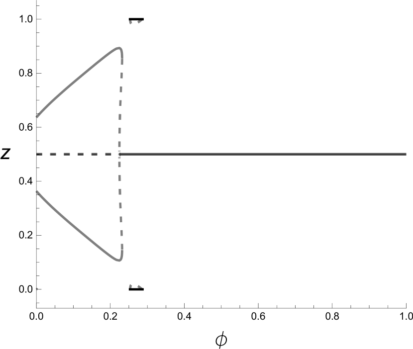
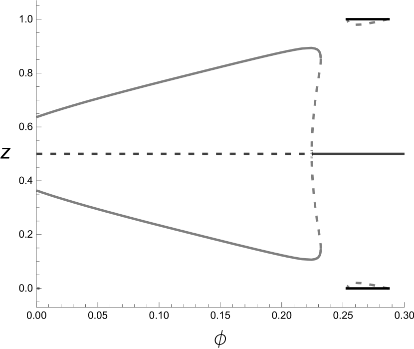
Figure 11: Bifurcation diagram for $(\lambda,\gamma,\sigma,b)=(1,0.9,8,0.1405)$. Filled lines correspond to stable equilbria and dashed lines correspond to unstable equilibria.

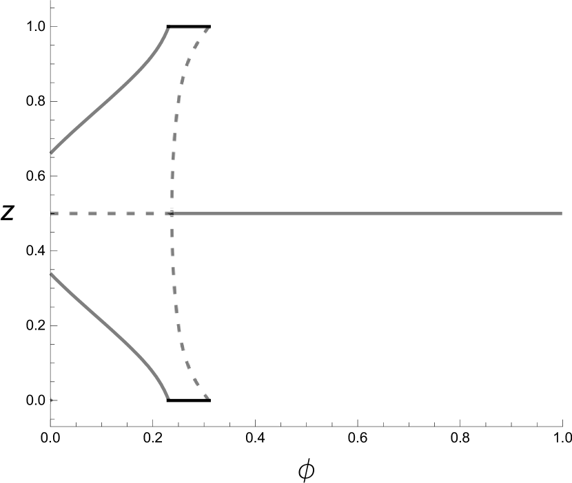
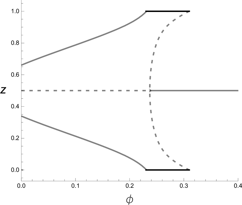
Figure 12: Bifurcation diagram for $(\lambda,\gamma,\sigma,b)=(1,0.9,8,0.15)$. Filled lines correspond to stable equilbria and dashed lines correspond to unstable equilibria.

In Figure 11 we set $b=0.146$, which is considerably lower than in the previously illustrated cases. We can observe that the re-dispersion process is quite different. Here, for very low levels of $\phi$ an asymmetric dispersion equilibrium exists and is stable, and becomes more asymmetric as $\phi$ increases. However, after a certain point, the economy starts to re-disperse until $\phi$ finds a limit point $\phi_{l}\in(\phi_{b2},1)$ above which the economy suddenly re-disperses evenly among the two regions. That is, the asymmetric dispersion undergoes a saddle-node bifurcation (refer to the end of Section 4 for a more detailed discussion) and there exists locational hysteresis as both an asymmetric dispersion equilibrium and the symmetric dispersion equilibrium are simultaneously stable for $\phi\in(\phi_{b2},\phi_{l})$. The symmetric equilibrium undergoes a subcritical pitchfork bifurcation at $\phi=\phi_{b2}$.

What is perhaps more striking though is that, as $\phi$ increases further, it encounters an interval $\phi\in(\phi_{s1},\phi_{s2})$ whereby both agglomeration and symmetric dispersion are stable, and a curve of unstable asymmetric equilibria exists in between. The striking feature is that the curve of agglomeration equilibria is not connected to any other kind of equilibrium.However, further increases in $b$ will eventually connect the asymmetric equilibrium curve with the full agglomeration as shown in Figure 12.This apparently strange behaviour may be attributed to the limitations imposed by the implicitly adopted asymptotic stability as the dynamic stability criterion in this paper. One way to investigate this issue could be to employ strategic stability as in Demichelis and Ritzberger, (2003), which entails additional necessary conditions for stability which restrict the equilibrium set. The potential game’s approach taken recently by Osawa and Akamatsu, (2020) could also be analysed in this context for equilibrium refinement. Finally, the connection via an increase in $b$ could hint at the existence of co-dimension $2$ bifurcations with $\phi$ and $b$ employed as bifurcation parameters. Although these are all relevant points, we do not pursue these issues further in our paper.

In Figure 12, we have $b=0.15$, and the economy reaches full agglomeration smoothly as $\phi$ increases but then jumps discontinuously to symmetric dispersion. We have the single breakpoint $\phi_{b2}\in(\phi_{s1},\phi_{s2})$, which means that there exists locational hysteresis as for $\phi\in(\phi_{b2},\phi_{s2})$ both agglomeration and symmetric dispersion are simultaneously stable.

Further increases in $b$ can be shown to lead, first to a situation similar to that of Figure 7, and then to ubiquitous agglomeration for any level of $\phi$.

Appendix C Results for Section 5

C.1 Existence and multiplicity of equilibria

Under this specification, the indirect utility is given by:

$$v_{i}^{S}=\frac{\mu\gamma}{\sigma}\left[z_{i}+cz_{j}\right]\left(\dfrac{\frac{\lambda}{2}+z_{i}}{z_{i}+\phi z_{j}}+\phi\dfrac{\frac{\lambda}{2}+z_{j}}{\phi z_{i}+z_{j}}\right)+\dfrac{\mu}{\sigma-1}\ln\left[z_{i}+\phi z_{j}\right]+\eta.$$ (25)

Differentiating $\Delta v^{S}(z)\equiv v_{1}^{S}(z)-v_{2}(z)^{S}$ twice with respect to $z$ yields:

$$\frac{d\Delta v^{S}}{dz}(z)=\frac{b_{1}P^{S}(z)}{b_{2}},$$

where:

$$b_{1} =\mu(2z-1)(\phi-1)$$

$$b_{2} =(\sigma-1)\sigma(z(\phi-1)+1)^{3}(z(\phi-1)-\phi)^{3},$$

and $P^{S}(z)$ is a second degree polynomial in $z.$ The zeros of $\frac{d\Delta v^{S}}{dz}(z)$ are the zeros of $P^{S}(z),$ which can be at most two. However, it is possible to check that $\frac{d\Delta v^{S}}{dz}(\frac{1}{2})=0.$ Given symmetry, no other real zero possibly exists. This means that $\Delta v^{S}(z)$ changes concavity only at symmetric dispersion. This implies that $\Delta v^{S}(z)$ has at most two turning points and thus, at most three equilibria. By symmetry, we can establish that there exists at most one equilibria for $z>\frac{1}{2}$.

Solving the condition for any (asymmetric) dispersion equilibrium is just as daunting a task as it is for the benchmark case, For the sake of brevity, let us just say that a dispersion equilibrium exists if $\lambda\equiv\lambda^{*S}(z)$, where $\lambda^{*S}(z)$ is a function of $z$ and all the parameters contained in the analogous expression in (23).

C.2 Stability of equilibria

First, let us analyze the stability of full agglomeration. Using (25), we get that agglomeration is stable if:

$$\mathcal{S}^{S}\equiv\frac{2(\lambda+1)\phi-c\left[(\lambda+2)\phi^{2}+\lambda\right]}{2\sigma\phi}-\frac{\ln\phi}{\sigma-1}>0.$$

It is readily observable that agglomeration is always stable if the first term is positive:

$$c>\frac{2(\lambda+1)\phi}{(\lambda+2)\phi^{2}+\lambda}.$$

We have:

$$\lim_{\phi\rightarrow 0}\mathcal{S}^{S}=-\infty\ \text{ and }\ \mathcal{S}(\phi=1)=\frac{(1-c)\gamma(\lambda+1)}{\sigma}>0.$$

Therefore, by the Intermediate Value Theorem, there exists at least one zero $\phi$ such that $\mathcal{S}=0.$ Further, we have:

$$\frac{d\mathcal{S}^{S}}{d\phi}=\frac{1}{\phi^{2}}\left(-\frac{c\gamma(\lambda+2)\phi^{2}}{\sigma}+\frac{c\gamma\lambda}{\sigma}-\frac{2\phi}{\sigma-1}\right),$$

whereby the term in parenthesis is a second degree polynomial with negative leading coefficient and that only changes sign once. Therefore, $\mathcal{S}^{S}$ has at most one turning point. Since $\frac{dS^{S}}{d\phi}(\phi=1)=\frac{1}{1-\sigma}-\frac{c\gamma}{\sigma}<0,$ we can conclude that the turning point is a maximum and $\mathcal{S}^{S}$ is strictly concave. Thus, there exists a unique sustain point $\phi_{s}^{S}\in(0,1)$ and agglomeration is stable when $\phi>\phi_{s}^{S}$

Second, we analyze the stability of symmetric dispersion. Using (25) it can be shown that $z^{*}=\frac{1}{2}$ is stable if:

$$\mathcal{B}^{S}\equiv-\gamma(\sigma-1)\left[\phi^{2}(c(2\lambda+3)+1)+2b\lambda+c-4(\lambda+1)\phi-1\right]+2\sigma\left(1-\phi^{2}\right)<0.$$ (26)

We can see that if the first term is positive, symmetric dispersion is always unstable, i.e., if:

$$c<\frac{\phi(4\lambda-\phi+4)+1}{(2\lambda+3)\phi^{2}+2\lambda+1}.$$

Moreover, $\mathcal{B}^{S}$ in (26) is a second degree polynomial with at most two zeros, $\phi_{b1}^{S}$ and $\phi_{b1}^{S}<\phi_{b2}^{S}$, with a negative leading coefficient, which means that symmetric dispersion is stable to the left of $\phi_{b1}^{S}$, unstable for $\phi\in\left(\phi_{b1}^{S},\phi_{b2}^{S}\right)$, and stable to the right of $\phi_{b2}^{S}$. However, it is possible to show after very cumbersome calculations that both break points cannot co-exist. As a result, we shall focus on the more interesting case, that is the stability around the first break point $\phi_{b1}^{S}$, which is given by:

$$\phi_{b1}^{S}= 2\gamma(\lambda+1)(\sigma-1)-$$

$$\frac{\sqrt{-(c+1)\gamma^{2}(\sigma-1)^{2}\left[c(4\lambda(\lambda+2)+3)-4\lambda(\lambda+2)-5\right]+4(c+1)\gamma\sigma(\sigma-1)+4\sigma^{2}}}{\gamma(\sigma-1)\left[c(2\lambda+3)+1\right]+2\sigma}.$$

Finally, we analyze the stability of (asymmetric) dispersion. Differentiating $\Delta v^{S}(z)$ with respect to $z$ and evaluating at $\lambda=\lambda^{*S}(z)$, we get that dispersion is stable if:

$$\mathcal{G}^{S}\equiv (2z-1)\left(\phi^{2}-1\right)\left[(c-1)\gamma(\sigma-1)(1-2z)^{2}-\sigma\right]+$$

$$+\sigma\left[2z^{2}(\phi-1)^{2}-2z(\phi-1)^{2}+\phi^{2}+1\right]\ln\left[\frac{z(\phi-1)+1}{z(1-\phi)+\phi}\right]<0.$$ (27)

C.3 Supercritical pitchfork bifurcation

We can get the whole picture of the dynamic properties of the model by studying the type of local bifurcation that the symmetric equilibrium undergoes at $\phi=\phi_{b1}^{S}.$ After some tedious calculations, it is possible to show the following:

$$\dfrac{\partial f}{\partial z}\left(\dfrac{1}{2};\phi_{b1}^{S}\right) =0;\ \dfrac{\partial^{2}f}{\partial z^{2}}\left(\dfrac{1}{2};\phi_{b1}^{S}\right)=0;\ \dfrac{\partial f}{\partial\phi}\left(\dfrac{1}{2};\phi_{b1}^{S}\right)=0$$

$$\dfrac{\partial^{2}f}{\partial\phi\partial z}\left(\dfrac{1}{2};\phi_{b1}^{S}\right) >0;\ \dfrac{\partial^{3}f}{\partial z^{3}}\left(\dfrac{1}{2};\phi_{b1}^{S}\right)<0.$$

According to Guckenheimer and Holmes, (2002, pp. 150), the conditions above ensure that symmetric dispersion undergoes a supercritical pitchfork bifurcation at $\phi=\phi_{b1}^{S}.$

References

- Aghion and Howitt, (1990) Aghion, P. and Howitt, P. (1990). A model of growth through creative destruction. Econometrica, pages 323–351.
- Aghion et al., (1998) Aghion, P., Howitt, P., and Howitt, P. W. (1998). Endogenous Growth Theory. MIT: MIT Press.
- Aizawa et al., (2020) Aizawa, H., Ikeda, K., Osawa, M., and Gaspar, J. M. (2020). Breaking and sustaining bifurcations in -invariant equidistant economy. International Journal of Bifurcation and Chaos, 30(16):2050240.
- Akamatsu et al., (2019) Akamatsu, T., Mori, T., Osawa, M., and Takayama, Y. (2019). Endogenous agglomeration in a many-region world. https://arxiv.org/abs/1912.05113.
- Akamatsu et al., (2012) Akamatsu, T., Takayama, Y., and Ikeda, K. (2012). Spatial discounting, Fourier, and racetrack economy: A recipe for the analysis of spatial agglomeration models. Journal of Economic Dynamics and Control, 99(11):32–52.
- Audretsch and Feldman, (1996) Audretsch, D. B. and Feldman, M. P. (1996). R&d spillovers and the geography of innovation and production. The American economic review, 86(3):630–640.
- Baldwin, (2016) Baldwin, R. (2016). The Great Convergence. Harvard University Press.
- Baldwin et al., (2003) Baldwin, R., Forslid, R., Martin, P., Ottaviano, G., and Robert-Nicoud, F. (2003). Economic Geography and Public Policy. Princeton University Press, Princeton.
- Barro and Sala-i Martin, (2004) Barro, R. J. and Sala-i Martin, X. (2004). Economic Growth. New York: McGraw-Hill.
- Baum-Snow, (2007) Baum-Snow, N. (2007). Did highways cause suburbanization? The Quarterly Journal of Economics, 122(2):775–805.
- Baum-Snow et al., (2017) Baum-Snow, N., Brandt, L., Henderson, J. V., Turner, M. A., and Zhang, Q. (2017). Roads, railroads, and decentralization of Chinese cities. Review of Economics and Statistics, 99(3):435–448.
- Behrens and Murata, (2021) Behrens, K. and Murata, Y. (2021). On quantitative spatial economic models. Journal of Urban Economics, 123:103348.
- Behrens and Robert-Nicoud, (2011) Behrens, K. and Robert-Nicoud, F. (2011). Tempora mutantur: In search of a new testament for neg. Journal of Economic Geography, 11(2):215–230.
- Berliant and Fujita, (2008) Berliant, M. and Fujita, M. (2008). Knowledge creation as a square dance on the Hilbert cube. International Economic Review, 49(4):1251–1295.
- Berliant and Fujita, (2009) Berliant, M. and Fujita, M. (2009). Dynamics of knowledge creation and transfer: The two person case. International Journal of Economic Theory, 5(2):155–179.
- Berliant and Fujita, (2011) Berliant, M. and Fujita, M. (2011). The dynamics of knowledge diversity and economic growth. Southern Economic Journal, 77(4):856–884.
- Berliant and Fujita, (2012) Berliant, M. and Fujita, M. (2012). Culture and diversity in knowledge creation. Regional Science and Urban Economics, 42(4):648–662.
- Bond-Smith, (2021) Bond-Smith, S. (2021). The unintended consequences of increasing returns to scale in geographical economics. Journal of Economic Geography, 21(5):653–681.
- Castro et al., (2021) Castro, S. B. S. D., da Silva, J. C., and Gaspar, J. M. (2021). Economic geography meets hotelling: the home-sweet-home effect. Economic Theory.
- Davis and Şener, (2012) Davis, L. S. and Şener, F. (2012). Private patent protection in the theory of schumpeterian growth. European Economic Review, 56(7):1446–1460.
- Demichelis and Ritzberger, (2003) Demichelis, S. and Ritzberger, K. (2003). From evolutionary to strategic stability. Journal of Economic Theory, 113(1):51–75.
- Dinopoulos and Segerstrom, (2010) Dinopoulos, E. and Segerstrom, P. (2010). Intellectual property rights, multinational firms and economic growth. Journal of Development Economics, 92(1):13–27.
- Dinopoulos and Segerstrom, (2006) Dinopoulos, E. and Segerstrom, P. S. (2006). North-south trade and economic growth.
- Duranton and Puga, (2001) Duranton, G. and Puga, D. (2001). Nursery cities: Urban diversity, process innovation, and the life cycle of products. American Economic Review, 91(5):1454–1477.
- Duranton and Puga, (2004) Duranton, G. and Puga, D. (2004). Micro-foundations of urban agglomeration economies. In Henderson, J. V. and Thisse, J.-F., editors, Handbook of Regional and Urban Economics, volume 4, pages 2063–2117. North-Holland.
- Duranton and Puga, (2015) Duranton, G. and Puga, D. (2015). Urban land use. In Duranton, G., Henderson, J. V., and Strange, W. C., editors, Handbook of Regional and Urban Economics, volume 5, pages 467–560. Elsevier.
- Forslid and Ottaviano, (2003) Forslid, R. and Ottaviano, G. I. (2003). An analytically solvable core-periphery model. Journal of Economic Geography, 3(3):229–240.
- Frenken et al., (2007) Frenken, K., van Oort, F., and Verburg, T. (2007). Related variety, unrelated variety and regional economic growth. Regional Studies, 41(5):685–697.
- Fujita, (2007) Fujita, M. (2007). Towards the new economic geography in the brain power society. Regional Science and Urban Economics, 37(4):482–490.
- Fujita et al., (1999) Fujita, M., Krugman, P., and Venables, A. (1999). The Spatial Economy: Cities, Regions, and International Trade. Princeton University Press.
- Fujita and Mori, (2005) Fujita, M. and Mori, T. (2005). Frontiers of the new economic geography. Papers in Regional Science, 84(3):377–405.
- Fujita and Thisse, (2013) Fujita, M. and Thisse, J. (2013). Economics of Agglomeration. Cambridge University Press.
- Gaspar, (2018) Gaspar, J. M. (2018). A prospective review on new economic geography. The Annals of Regional Science, 61(2):237–272.
- Gaspar, (2020) Gaspar, J. M. (2020). New economic geography: history and debate. The European Journal of the History of Economic Thought, pages 1–37.
- Gaspar et al., (2018) Gaspar, J. M., Castro, S. B., and Correia-da Silva, J. (2018). Agglomeration patterns in a multi-regional economy without income effects. Economic Theory, 66(4):863–899.
- Gaspar et al., (2021) Gaspar, J. M., Ikeda, K., and Onda, M. (2021). Global bifurcation mechanism and local stability of identical and equidistant regions: Application to three regions and more. Regional Science and Urban Economics, 86:103597.
- Guckenheimer and Holmes, (2002) Guckenheimer, J. and Holmes, P. (2002). Nonlinear oscillations, dynamical systems, and bifurcations of vector fields. Number 42 in Applied mathematical sciences. Springer, New York, 7th edition.
- Helpman, (1998) Helpman, E. (1998). The size of regions. In Pines, D., Sadka, E., and Zilcha, I., editors, Topics in Public Economics: Theoretical and Applied Analysis, pages 33–54. Cambridge University Press.
- Howitt, (1999) Howitt, P. (1999). Steady endogenous growth with population and r. & d. inputs growing. Journal of Political Economy, 107(4):715–730.
- Ikeda et al., (2012) Ikeda, K., Akamatsu, T., and Kono, T. (2012). Spatial period-doubling agglomeration of a core–periphery model with a system of cities. Journal of Economic Dynamics and Control, 36(5):754–778.
- Jones, (1995) Jones, C. I. (1995). Time series tests of endogenous growth models. The Quarterly Journal of Economics, 110(2):495–525.
- Kleinman et al., (2023) Kleinman, B., Liu, E., and Redding, S. J. (2023). The linear algebra of economic geography models. Technical report, National Bureau of Economic Research.
- (43) Krugman, P. (1991a). Geography and trade. MIT press.
- (44) Krugman, P. (1991b). Increasing returns and economic geography. Journal of Political Economy, 99(3):483–499.
- Krugman, (2011) Krugman, P. (2011). The new economic geography, now middle-aged. Regional studies, 45(1):1–7.
- Krugman and Venables, (1995) Krugman, P. R. and Venables, A. J. (1995). Globalization and the inequality of nations. The Quarterly Journal of Economics, 110(4):857–880.
- Li, (2003) Li, C.-W. (2003). Endogenous growth without scale effects: A comment. American Economic Review, 93(3):1009–1017.
- Osawa and Akamatsu, (2020) Osawa, M. and Akamatsu, T. (2020). Equilibrium refinement for a model of non-monocentric internal structures of cities: A potential game approach. Journal of Economic Theory, 187(C).
- Osawa and Gaspar, (2021) Osawa, M. and Gaspar, J. M. (2021). Production externalities and dispersion process in a multi-region economy.
- Ottaviano and Peri, (2006) Ottaviano, G. I. and Peri, G. (2006). The economic value of cultural diversity: Evidence from US cities. Journal of Economic geography, 6(1):9–44.
- Ottaviano and Peri, (2008) Ottaviano, G. I. and Peri, G. (2008). Immigration and national wages: Clarifying the theory and the empirics. Technical report, National Bureau of Economic Research.
- Ottaviano and Prarolo, (2009) Ottaviano, G. I. and Prarolo, G. (2009). Cultural identity and knowledge creation in cosmopolitan cities. Journal of Regional Science, 49(4):647–662.
- Peretto, (1998) Peretto, P. F. (1998). Technological change and population growth. Journal of Economic Growth, 3(4):283–311.
- Peretto, (2012) Peretto, P. F. (2012). Resource abundance, growth and welfare: A Schumpeterian perspective. Journal of Development Economics, 97(1):142–155.
- Peretto, (2015) Peretto, P. F. (2015). From Smith to Schumpeter: A theory of take-off and convergence to sustained growth. European Economic Review, 78:1–26.
- Pflüger, (2004) Pflüger, M. (2004). A simple, analytically solvable, chamberlinian agglomeration model. Regional science and urban economics, 34(5):565–573.
- Pflüger and Südekum, (2008) Pflüger, M. and Südekum, J. (2008). Integration, agglomeration and welfare. Journal of Urban Economics, 63(2):544–566.
- Pflüger and Tabuchi, (2010) Pflüger, M. and Tabuchi, T. (2010). The size of regions with land use for production. Regional Science and Urban Economics, 40(6):481–489.
- Picard, (2015) Picard, P. M. (2015). Trade, economic geography and the choice of product quality. Regional Science and Urban Economics, 54:18–27.
- Proost and Thisse, (2019) Proost, S. and Thisse, J.-F. (2019). What can be learned from spatial economics? Journal of Economic Literature, 57(3):575–643.
- Puga, (1999) Puga, D. (1999). The rise and fall of regional inequalities. European Economic Review, 43(2):303–334.
- Redding and Rossi-Hansberg, (2017) Redding, S. J. and Rossi-Hansberg, E. (2017). Quantitative spatial economics. Annual Review of Economics, 9:21–58.
- Robert-Nicoud, (2008) Robert-Nicoud, F. (2008). Offshoring of routine tasks and (de) industrialisation: Threat or opportunity–and for whom? Journal of urban Economics, 63(2):517–535.
- Romer, (1990) Romer, P. M. (1990). Endogenous technological change. Journal of political Economy, 98(5, Part 2):S71–S102.
- Storper, (2011) Storper, M. (2011). Why do regions develop and change? the challenge for geography and economics. Journal of economic geography, 11(2):333–346.
- Tabuchi, (1998) Tabuchi, T. (1998). Urban agglomeration and dispersion: A synthesis of alonso and krugman. Journal of Urban Economics, 44(3):333–351.
- Tabuchi, (2014) Tabuchi, T. (2014). Historical trends of agglomeration to the capital region and new economic geography. Regional Science and Urban Economics, 44:50–59.
- Tabuchi and Thisse, (2011) Tabuchi, T. and Thisse, J.-F. (2011). A new economic geography model of central places. Journal of Urban Economics, 69(2):240–252.
- Tavassoli and Carbonara, (2014) Tavassoli, S. and Carbonara, N. (2014). The role of knowledge variety and intensity for regional innovation. Small Business Economics, 43(2):493–509.
- Venables, (1996) Venables, A. J. (1996). Equilibrium locations of vertically linked industries. International Economic Review, pages 341–359.
- Young, (1998) Young, A. (1998). Growth without scale effects. Journal of Political Economy, 106(1):41–63.