How to Train Your Gyro:
Reinforcement Learning for Rotation Sensing with a Shaken Optical Lattice

Abstract

As the complexity of the next generation of quantum sensors increases, it becomes more and more intriguing to consider a new paradigm in which the design and control of metrological devices is supported by machine learning approaches. In a demonstration of such a design philosophy, we apply reinforcement learning to engineer a shaken-lattice matter-wave gyroscope involving minimal human intuition. In fact, the machine is given no instructions as to how to construct the splitting, reflecting, and recombining components intrinsic to conventional interferometry. Instead, we assign the machine the task of optimizing the sensitivity of a gyroscope to rotational signals and ask it to create the lattice-shaking protocol in an end-to-end fashion. What results is a machine-learned solution to the design task that is completely distinct from the familiar sequence of a typical Mach-Zehnder-type matter-wave interferometer, and with significant improvements in sensitivity.

If one asks an expert for advice as to how to measure tiny displacements or forces over large distances, they will likely point to the very large body of literature on interferometry, perhaps highlighting LIGO [1] and other such remarkable interferometry systems [2]. Optical interferometers are not the only ones useful in high precision measurements, and indeed matter-wave interferometers have also offered the potential for exquisite sensitivity to inertial forces [3, 4]. In the work by Weidner et al., a new kind of matter-wave interferometric accelerometer that utilizes an optical lattice was proposed and demonstrated experimentally [5, 6, 7]. The purpose of the optical lattice is to provide robustness of the system in the face of a harsh dynamical environment typical of real-world applications [8, 9]. It has been demonstrated that the quantum design of optical-lattice-based interferometers can benefit greatly from machine learning approaches, since the machine can search an extensive number of possible control protocols systematically and come up with one that is not intuitive but very effective. The earlier work established that one can ‘teach’ the system to become sensitive to acceleration by learning how to modulate the phase of the lattice with unconventional patterns, that is, how to shake the lattice such that the system carries out an interferometric protocol [10].

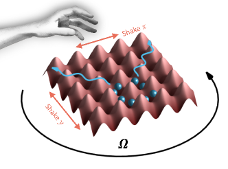
Figure 1: A two-dimensional optical lattice potential in a rotating frame, where atoms are trapped and their dynamics can be controlled by an external agent (the hand) shaking the lattice. The blue arrows indicate possible trajectories associated with splitting of the matterwaves.

While this work demonstrated the power of machine learning to construct a device to surpass conventional Bragg interferometry, the machine learning was constrained, let us say, by the expert’s understanding of how interferometry is to take place. Indeed, nearly every kind of interferometry, optical or matter wave, takes place as a sequence of wavefront splitting, reflection, and recombination, with wave propagation in between, known as the Mach-Zehnder configuration [11, 12]. If we free the learning agent from being restricted by conventional wisdom, it may then potentially discover solutions that surpass what humans have explored to date. For example, Ref. [13] has shown that an active-learning agent can predict novel configurations for quantum optics experiments that generate highly-entangled states.

In this paper, we present results from the application of machine learning to quantum metrology, specifically to train a two-dimensional optical lattice to sense rotation with high precision and thereby embody the design objectives of a gyroscope. Our goal is to build a better, more sensitive gyroscope, with an optical lattice providing the skeletal framework to support the ultracold atoms, as depicted in Fig. 1. The type of machine learning we employ is known as reinforcement learning [14], the aim of which is to maximize long-term rewards of a control protocol in situations where the optimal solution is not transparent at each individual step. In contrast to the component design for the accelerometer [10], here we utilize reinforcement learning in a manner that removes the prejudice of an expert as to how interferometry is supposed to be done. Instead, learning is driven purely by performance metrics—that is, what it means to be a good gyroscope rather than what it means to be a proper interferometer. Moreover, the machine learning can navigate a trade-space of criteria, such as a combination of sensitivity, dynamic range, and tolerance to noise and experimental drifts, as motivated by the task at hand.

The system we consider is one where the atoms are confined in a two-dimensional optical lattice. The lattice in each dimension can be ‘shaken’ by varying the phases of the corresponding pairs of interfering laser beams. The entire system is described mathematically in a rotating non-inertial frame by the Hamiltonian

$$\hat{H}=\frac{\hat{\vectorsym{p}}^{2}}{2m}-\vectorsym{\Omega}\cdot\hat{\vectorsym{L}}-\sum_{\alpha\in\{x,y\}}\frac{V_{\alpha}}{2}\cos(2k\hat{\alpha}+\phi_{\alpha})\,,$$ (1)

where $m$ is the mass of a single atom with coordinate $\hat{\vectorsym{r}}=\{\hat{x},\hat{y}\}$ and momentum $\hat{\vectorsym{p}}$, $k$ is the laser wavenumber, $\phi_{\alpha}$’s are the phase differences between the two counter-propagating lasers in the $x$ or $y$ directions, and $V_{\alpha}$’s are the corresponding lattice potential strengths. The term $\vectorsym{\Omega}\cdot\hat{\vectorsym{L}}$ describes the rotational kinetic energy of the system, with $\hat{\vectorsym{L}}=\hat{\vectorsym{r}}\times\hat{\vectorsym{p}}$ the angular momentum, and $\vectorsym{\Omega}$ the angular velocity. It is the unknown magnitude, $\Omega$, that is the metrological parameter that we wish to measure with high accuracy.

For reference, we first derive a conventional two-path Sagnac matter-wave interferometer, motivated by the fiberoptic gyroscope [15], but implemented with atoms [16, 17, 18]. This can be constructed in the lattice using the previously developed beam-splitting and reflecting protocols that were based on components optimized by reinforcement learning [10]. The splitting protocol was demonstrated to transfer the ground state to an approximate superposition of the $\ket{\pm 4\hbar k}$ states, and the reflecting protocol to map any linear combination of the $\ket{\pm 4\hbar k}$ states to the corresponding combination of the $\ket{\mp 4\hbar k}$ states. In order to build a gyroscope from these components, as illustrated in Fig. 2(a), the sequence of operations is the following:

• Initially, the wavefunction is prepared in the ground state of the 2D lattice.

• In the $x$-direction, the 1D beam-splitting protocol is applied, allowing free propagation for a duration, denoted as $T$, and then the reflecting protocol is applied. Following this, free propagation occurs for a duration $2T$, and then the reflecting protocol is applied again, followed by free propagation for a duration $T$, and finally the recombining protocol.

• In the $y$-direction, the lattice operates as a conveyor belt for the trapped atoms. The lattice is smoothly accelerated to the velocity $4\hbar k/m$ according to the adiabaticity criterion, as described in the Supplemental Material (SM), and then translated at constant velocity. During the halfway point of the sequence, when the two paths in the $x$-directions cross, the velocity of the $y$-lattice is decelerated through zero to $-4\hbar k/m$, so that the lattice can be translated backward at the constant velocity. The final step is to adiabatically accelerate the $y$-lattice back to zero velocity for the final recombination protocol.

Such a device operates on the principle of the Sagnac effect, which describes the phase difference, $\Delta\phi$, that accumulates between two waves that propagate in opposite directions in a loop when in a non-inertial rotating frame. In general, the phase difference is proportional to both the angular velocity and to the area that the two paths enclose, $\vectorsym{A}$. In the case of matter-waves, $\Delta\phi=4m\vectorsym{\Omega}\cdot\vectorsym{A}/\hbar$ [19, 20]. If higher sensitivity is desired, one could effectively increase $\vectorsym{A}$ by completing many cycles before applying the last recombination step. In practice, it is often the case that one needs to balance multiple cycles against any reduced fringe visibility that may arise from imperfections.

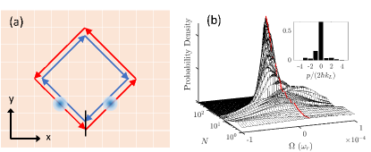
Figure 2: (a) The clockwise trajectory (blue) and the counter-clockwise trajectory (red) taken by the wave functions in the two-path shaken lattice gyroscope. The vertical back line is where the wave functions were initially split and are eventually recombined. (b) Bayesian reconstruction of the rotation rate from the interference patterns generated by the two-path gyroscope. The main plot shows the probability distribution of the estimated rotation rate for numbers of measurements ranging from 1 to 500. The red curve indicates the true value of the rotation rate, which is $2\times 10^{-4}~{}\omega_{r}$ where $\omega_{r}=\hbar k^{2}/(2m)$. At 500 measurements, the peak of the distribution coincides with the true value, meaning that the estimation is unbiased. The inset shows the momentum distribution output at a rotation rate of $2\times 10^{-4}~{}\omega_{r}$.

Given this reference system, we now consider the possibility for a completely end-to-end design that is not based on the decomposition into components. We implement the machine learning for this overarching design goal by employing the double-deep-Q approach [21], the algorithm for which is described in detail in Ref. [10]. In overview, this reinforcement learning algorithm consists of an agent that selects actions based on the observed state of the environment, and an environment that carries out the the action and generates a consequential reward based on the observed quality of the resulting state. The agent does not need to be exposed to the full quantum state, but only to relevant features of that state, such as the population in the discrete momentum basis in $x$ and the average position and momentum in $y$.

Motivated in part by potential experimental implementation, we choose the actions to be selected from a finite set of discrete options for the time derivative of the phase, i.e., $\partial\phi/\partial t$. This represents a frequency difference between interfering laser beam pairs. The wave packet evolution that this generates is calculated by numerical solution of the time-dependent Schrödinger equation, using a separation ansatz for the $x$ and $y$ dimensions (see SM). In order to compute the reward, we use the classical Fisher information [22], which quantitatively measures the sensitivity. To do this, we replicate the environment as three copies of the quantum system with slightly different rotation rates, $\Omega=[\Omega_{0}-d\Omega,\,\Omega_{0},\,\Omega_{0}+d\Omega]$, for small $d\Omega$ and with each evolving according to Eq. (1). This construction allows us to compute the derivative with respect to $\Omega$ by numerical symmetric finite differencing. The classical Fisher information is given by

$$I_{1}(\Omega)=\sum_{p}\frac{1}{\mathrm{Pr}(p|\Omega)}\left[\frac{\partial\mathrm{Pr}(p|\Omega)}{\partial\Omega}\right]^{2}\,,$$ (2)

where $\mathrm{Pr}(p|\Omega)$ is the probability for measuring a momentum $p$ at the gyroscope output for the given $\Omega$. Reinforcement learning aims to generate steps that maximize the long-term reward, that is, to find a sequence of $\partial\phi/\partial t$ steps that optimizes the Fisher information evaluated at the terminal time. The potential sensitivity is constrained by a theoretical bound (Cramér-Rao bound) for the standard deviation of the measurement,

$$\sigma_{\Omega}\geq 1/\sqrt{NI_{1}(\Omega)},$$ (3)

where $N$ is the number of independent measurements (atoms). Here we have optimized for a specific choice of the angular frequency, $\Omega_{0}$, but straightforward extensions are possible, including designing for performance over a finite range.

Within the context of our learning framework, we are able to obtain lattice shaking protocols that outperform the conventional two-path gyroscope. The solution varies for every instantiation due to the randomized initialization of the agent. The illustration in Fig. 3 shows one of the realized machine-learned protocols that gives high sensitivity. The pattern is reminiscent of speckle patterns that emerge from a multi-mode fiber (fiber specklegram), which are known to be sensitive interference detectors of inertial phase. However, in the case of a multi-mode fiber system, the patterns are not robust and are scrambled by temperature changes or strain on the fiber. The situation is quite different here, since the adverse noise and imperfections that may enter are different in origin and primarily common-mode. Despite the non-trivial and irregular pattern, this device will measure rotation signals with high accuracy, which we now demonstrate by simulating an example measurement record.

The momentum distributions that are produced by the multi-path interferometer under conditions of different values of the rotation rate are shown in Fig. 4. The population of each momentum component is indicated by false color. The more detailed structure there is in the momentum distribution as the rotation rate is varied, the more sensitive is the interferometer. Note that each vertical slice is essentially unique, and therefore the momentum distribution acts as a fingerprint that allows one to infer the rotation rate without aliasing. The Fisher information calculated from the distribution is also shown in Fig. 4. The value on the $y$-axis is the ratio between the Fisher information from this multi-mode interferometer and the one shown previously based on the two-path arrangement. We optimize the Fisher information around $\Omega_{0}=0$, and one can see that the Fisher information is maximum at $\Omega=0$, with large dynamic range being sacrificed for high sensitivity.

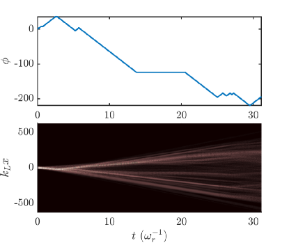
Figure 3: Evolution of the phase function and the spatial wavefunction. The shaking protocol was generated from the reinforcement learning agent with $\partial\phi/\partial t$ as the actions in an end-to-end design. There are 125 discrete steps in this protocol. The wavefunction was initialized in the ground state of the lattice convolved with a momentum width $\sigma_{p}=0.1\,\hbar k$, and then evolved according to the shaking protocol given.

The machine-learned gyroscope achieved a Fisher information of around 25 times higher than the two-path gyroscope shown earlier in this paper, meaning that the sensitivity is improved by the square root of this, or a factor of 5. In other words, the interferometer is effectively as sensitive as a conventional one that is 5 times larger. If we make a comparison to the gyroscope with the same footprint constructed from Bragg interferometry, the improvement is $4\times 5=20$-fold. The extra factor of 4 introduced here is primarily due to large angle splitting, $8\hbar k$ instead of $2\hbar k$, and was demonstrated in Ref. [10]. This significant potential gain is remarkable and demonstrates the scope for improvements upon current state-of-the-art approaches.

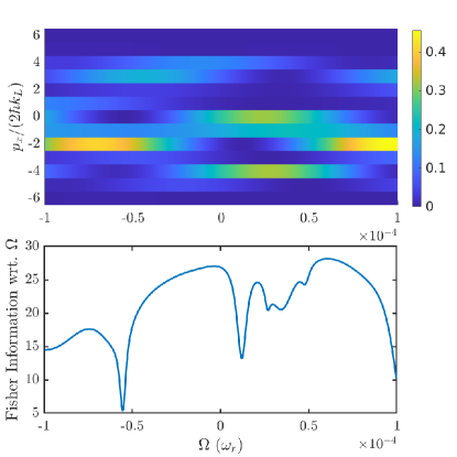
Figure 4: Population distribution in the momentum basis and the resulting classical Fisher information for the machine-learned shaken-lattice gyroscope as a function of the rotation rate $\Omega$. The value of the Fisher information is normalized by the Fisher information for the two-path interferometer, which has splitting of order $\Delta p=8\hbar k$, and thus sensitivity about 4 times better than a conventional Bragg interferometer.

To extract the rotational signal from the distribution shown in Fig. 4, we apply Bayesian reconstruction [23]. This means that we iteratively update the prior distribution for $\Omega$ from each atom measurement. The reconstruction of the rotational signal is shown in Fig. 5(a), and note that the peak coincides with the true rotation rate as indicated by the red line, thereby verifying that the estimation for $\Omega$ is unbiased. In Fig. 5(b), we plot the standard deviation of $\Omega$, and see that the sensitivity scales inversely with the square root of the number of atoms, as expected from independent measurements.

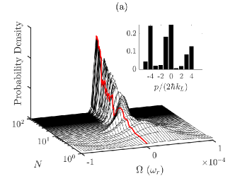
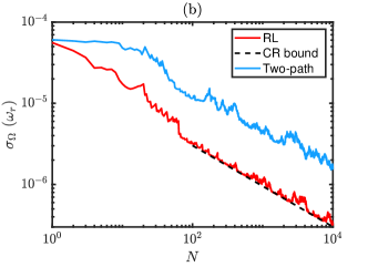
Figure 5: (a) An example Bayesian reconstruction of the rotation rate, showing the probability distribution for sampling 1 atom to 100 atoms. The true rotation value is indicated by the red line, and the inset shows the shaken lattice interferometer output distribution for this value. (b) The standard deviation of the rotation rate as a function of the atom number (RL, red curve). The result at large atom number is consistent with the Cramér-Rao (CR, dotted line) bound. The performance greatly surpasses the two-path inteferometer shown earlier (Two-path, blue curve).

In conclusion, we have proposed and analyzed the efficacy of the use of deep reinforcement learning for the optimization of a quantum sensor. We have demonstrated the explicit application of this concept through an example of the design of a shaken-lattice matter-wave gyroscope. We first showed that a Mach-Zehnder-type matter-wave gyroscope can be constructed in a 2D lattice from a conveyor belt in the $y$-direction and the previously developed beam-splitting and reflecting shaking functions in the $x$-direction. We then applied reinforcement learning in an end-to-end fashion to find a shaking protocol that improved the sensitivity of the gyroscope by a factor of 5 when compared to the conventional Mach-Zehnder interferometry, and a factor of 20 when compared to Bragg interferometry. These results demonstrate the exceptional potential of the learning approach and open up the possibility for applying the same principal machinery to a variety of quantum sensing problems with more complex landscapes, such as multi-parameter estimation and entanglement-enhanced metrology. Furthermore, the implications of our results may go beyond this framework, and the same ideas of reinforcement learning may be applied to a variety of quantum and classical systems where the design of complex circuits for algorithmic tasks is needed.

The authors acknowledge helpful discussions with Joshua Combes, Marco Nicotra, Penny Axelrad, Catherine Catie LeDesma and Kendall Mehling. This work was supported by NSF OMA 1936303, NSF PHY 2207963, NSF OMA 2016244, and NSF PHY 1734006.

Supplemental Materials: How to Train Your Gyro:
Reinforcement Learning for Rotation Sensing with a Shaken Optical Lattice

S 1 Control and dynamics in the $y$-direction

The evolution of the wave function in the $y$-direction can be simple providing the strength of the $y$-optical lattice is sufficiently large. The transport of the lattice in the $y$-direction in this case carries the atomic wavepacket along with it, acting essentially as a conveyor belt. During the splitting in the $x$-direction, the $y$-lattice is accelerated uniformly to velocity $+4\hbar k/m$, and then remains for some time at this constant velocity. During the halfway point of the gyroscope cycle, the lattice is decelerated uniformly to cross zero velocity and then reaches constant velocity $-4\hbar k/m$, again for some time. At the recombination stage, the lattice is accelerated forward from this negative value to reach zero velocity. The resulting average position, $\expectationvalue{\hat{y}}$ and the average momentum, $\expectationvalue{\hat{p}}$, of the wavepacket are shown in Fig. S1. The oscillations in the momentum plot are due to the atoms being trapped in the bottom of the lattice sites, which are close to harmonic traps, and the acceleration stage being not perfectly adiabatic.

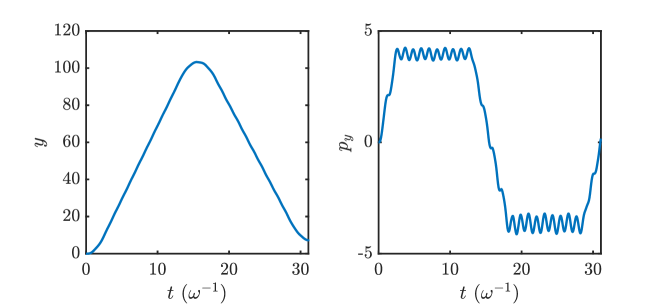
Figure S1: Left: Average position of the wavepacket in the $y$-direction. Right: Average momentum of the wavepacket in the $y$-direction. The lattice depth $V_{y}$ is set to $10~{}\hbar\omega_{r}$.

S 2 Effective 1D model

One of the challenges of simulating the two-dimensional rotating lattice is that, in general, the time complexity scales quadratically with the number of momentum states. To enable efficient simulations, which is especially important when running a very large number of machine-learning episodes, we reduce the system computation to a linear complexity by introducing an approximation of a deep $y$-potential lattice. This means that we take advantage of the fact that when a deep lattice in the $y$-direction is adiabatically translated, the shape of the wavepacket in the $y$-direction is approximately unchanged and is simply transported along with the lattice. This approximation is encapsulated by a separable ansatz, where we assume the two-dimensional wavefunction can be well represented as the tensor product of separable wavefunctions in the $x$ and $y$ directions, i.e.,

$$\ket{\psi} \approx \ket{\psi_{x}}\otimes\ket{\psi_{y}}\,,$$

$$\hat{p}_{y} \approx \langle\hat{p}_{y}\rangle\,,$$

$$\hat{y} \approx \langle\hat{y}\rangle\,.$$ (1)

With this ansatz, the time-dependent solution and the interference that is formed is determined soley by the $x$-direction evolution, as described by

$$\widetilde{H}_{x} = \frac{\hat{p}_{x}}{2m}-\frac{V_{0}}{2}\cos(2k\hat{x}+\phi_{x})-\Omega\widetilde{L}_{z}\,,$$ (2)

where $\widetilde{L}_{z}=\big{(}\langle\hat{p}_{y}\rangle\hat{x}-\langle\hat{y}\rangle\hat{p}_{x}\big{)}$. The mean position and momentum in the $y$-direction for the sequence just described was shown in Fig. S1. The conditions for the validity of the separation ansatz are further discussed in the following section. The simulations for the reinforcement learning environment are carried out under the effective 1D assumption, where only the dynamics in $x$-direction is important for the device behavior.

S 2.1 Evaluating the validity of the separable ansatz

We can write the 2D wavefunction in the form of its Schmidt decomposition,

$$\psi(x,y)=\sum_{i}\sqrt{p^{(i)}}\ \psi_{x}^{(i)}(x)\,\psi_{y}^{(i)}(y)$$ (3)

This decomposition can be obtained numerically from singular value decomposition. If the highest singular value $p^{(0)}$ is close to identity, we can drop the other terms in the summation, and approximate the 2D wavefunction as the separable form, i.e.,

$$\psi(x,y)\approx\psi_{x}^{(0)}(x)\,\psi_{y}^{(0)}(y)$$ (4)

To verify that in the case where the $y$-wavepacket is adiabatically transported along the lattice, the approximation shown above is valid, we compute the Schmidt decomposition of the 2D wavefunction evolved from the full 2D Hamiltonian. For the parameters presented in this paper, we find the highest singular value is of order $0.95$. In Fig. 2, we compare the population distribution in $x$ from the full 2D wavefunction, $|\psi_{2D}(x)|^{2}=\int|\psi(x,y)|^{2}\,dy$, and that from the Schmidt decomposition, $|\psi_{x}^{(0)}(x)|^{2}$.

The validity of the approximation allows us to universally apply the separable ansatz in the regime of our study, i.e., $\psi_{\mathrm{sep}}(x,y)=\psi_{x}(x)\psi_{y}(y)$, and evolve the wavefunctions in the $x$ and $y$ directions separately using the effective 1D Hamiltonians.

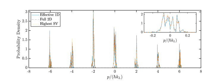
Figure S2: Comparison between the simulation results of the final probability distributions in the $x$ direction for the effective 1D model (blue), the full 2D model (orange dash), and the highest singular value component from the 2D model (yellow dotted). The inset shows a magnified view of the region around zero momentum. As this example demonstrates, the probability distributions all agree well for our parameters, justifying the use of the separation ansatz for our studies.

S 2.2 Adiabaticity in the accelerating lattice conveyor belt

In this section, we investigate the adiabaticity condition for the wavefunction to stay in the ground state of an accelerating lattice. The Hamiltonian in the $y$-direction in the lab frame is

$$\hat{H}_{y}=\frac{\hat{p}_{y}}{2m}-\frac{V_{y}}{2}\cos\big(2k\hat{y}+\phi(t)\big{missing})\,.$$ (5)

With the unitary transform given by the operator

$$\hat{U}=\exp\big(-i\hat{p}_{y}\phi/2\hbar k\big{missing})\,,$$ (6)

we move into the frame that is co-moving with the lattice. The Hamiltonian in the co-moving frame is

$$\hat{\widetilde{H}}_{y}=\frac{\hat{p}_{y}}{2m}-\frac{V_{y}}{2}\cos\big(2k\hat{y}+\phi(t)\big{missing})+\frac{1}{2k}\frac{d\phi}{dt}\hat{p}_{y}$$ (7)

The instantaneous eigenstates are

$$\ket{\widetilde{\psi}_{N,q}}=\exp(\frac{im\hat{y}\frac{d\phi}{dt}}{2\hbar k})\,\exp\big(-\frac{i\hat{p}\phi}{2\hbar k}\big{missing})\ket{\psi_{N,q}}\,,$$ (8)

where $\ket{\psi_{N,q}}$ are the Bloch eigenstates with band index $N$ and quasimomentum $q$. If we wish to ensure that the wavefunction stays in the ground state ($N=0$), then the quantum adiabatic theorem requires that

$$\sum_{m\neq 0}\bigg{|}\frac{\hbar\bra{m}\dot{\widetilde{H}}\ket{0}}{(E_{m}-E_{n})^{2}}\bigg{|}=\sum_{m\neq 0}\bigg{|}\frac{\hbar\bra{m}\hat{p}\,\ddot{\phi}/2k\ket{0}}{(E_{m}-E_{n})^{2}}\bigg{|}\ll 1\,.$$ (9)

For $V_{y}=10\,E_{r}$, numerical calculations show that the adiabaticity condition is $|\ddot{\phi}|\ll 60\,\omega_{r}^{2}$. In our simulations, we use $|\ddot{\phi}|=6.4\,\omega_{r}^{2}$, which satisfies the adiabaticity condition.

S 3 Fisher information for the two-path interferometer

The sensitivity of the gyroscope constructed using the splitting and reflecting protocols is presented in terms of the Fisher information in Fig. S3. Note that the value of the Fisher information is normalized to unity for an ideal two-path gyroscope with the same momentum splitting and free-propagation duration as the one we construct, i.e.,

$$I_{\mathrm{Sagnac}}=\bigg{[}\frac{4m}{\hbar}\left(\frac{2p_{0}^{2}T^{2}}{m^{2}}\right)\bigg{]}^{2}$$ (10)

where $p_{0}=4\hbar k$, and we have set $T=10~{}m/\hbar k^{2}$. The shaken lattice gyroscope gives a Fisher information of order unity as can be anticipated, and the slight deviation is due to imperfections in the components and the fact that the shaken lattice is does not fit perfectly within the two-path framework.

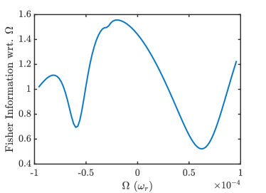
Figure S3: The Fisher information as a function of the rotation rate $\Omega$. The Fisher information of the gyroscope in which the matter waves follow the ideal paths of a diamond is normalized to unity.

S 4 Reinforcement learning for the gyro design

S 4.1 States and Actions

The features of the quantum state given to the reinforcement learning agent consists of information about the populations in $\{\ket{2n\hbar k}|n=\pm 3,\pm 2,\pm 1,0\}$ in the $x$-direction and the position and momentum in the $y$-direction. It is represented by the vector,

$$s=\left[P_{-3},\ P_{-2},\ P_{-1},\ P_{-0},\ P_{-1},\ P_{-2},\ P_{-3},\frac{\expectationvalue{\hat{y}}}{40},\frac{\expectationvalue{\hat{p}_{y}}}{4}\right]\,,$$ (11)

where $P_{n}$ represents the populations in the $\ket{2n\hbar k}$ states. The actions are implemented as the time derivatives of the laser phase in the $x$-direction as selected from a discrete set of possible values,

$$\mathcal{A}\in\{-\dot{\phi}=-8,\ \dot{\phi}=0,\ \dot{\phi}=8\}.$$ (12)

S 4.2 Hyperparameters of the neural network and training

This section outlines the hyperparameters that we use for training the double deep Q-learning agent. The parameter $\gamma$ stands for the discount factor, $\tau$ is the update rate of the target network, $\alpha$ denotes the learning rate. The exploration rate $\epsilon$ decays from $1$ to $0.008$ linearly at a rate given by $\epsilon$-decay. The neural network we use has two hidden layers, each with 64 nodes and are fully connected. The batch size represents the number of samples we average over for every learning step. The optimizer we use is the stochastic gradient descent (SGD), with momentum set to 0.5.

Hyperparameters	Values
$\gamma$	0.992
$\tau$	0.9985
$\alpha$	0.0005
$\epsilon$-decay	0.004
episodes	2,500
Hidden layers	64 $\times$ 64
Batch size	128
Optimizer	SGD

Table 1: Choice of hyperparameters for the gyroscope optimization task using double deep Q-learning.

References

- Abbott et al. [2016] B. P. Abbott et al. (LIGO Scientific Collaboration and Virgo Collaboration), Phys. Rev. Lett. 116, 061102 (2016).
- Acernese et al. [2007] F. Acernese, P. Amico, M. Al-Shourbagy, et al., Optics and Lasers in Engineering 45, 478 (2007).
- Bordé [1989] C. Bordé, Physics Letters A 140, 10 (1989).
- Kasevich and Chu [1991] M. Kasevich and S. Chu, Phys. Rev. Lett. 67, 181 (1991).
- Weidner et al. [2017] C. A. Weidner, H. Yu, R. Kosloff, and D. Z. Anderson, Phys. Rev. A 95, 043624 (2017).
- Weidner and Anderson [2018a] C. A. Weidner and D. Z. Anderson, Phys. Rev. Lett. 120, 263201 (2018a).
- Weidner and Anderson [2018b] C. A. Weidner and D. Z. Anderson, New Journal of Physics 20, 075007 (2018b).
- Xu et al. [2019] V. Xu, M. Jaffe, C. D. Panda, S. L. Kristensen, L. W. Clark, and H. Müller, Science 366, 745 (2019).
- Nelson et al. [2020] K. D. Nelson, C. D. Fertig, P. Hamilton, J. M. Brown, B. Estey, H. Müller, and R. L. Compton, Applied Physics Letters 116, 234002 (2020).
- Chih and Holland [2021] L.-Y. Chih and M. Holland, Phys. Rev. Research 3, 033279 (2021).
- Mach [1892] L. Mach, Zeitschrift für Instrumentenkunde 12, 89 (1892).
- Zehnder [1891] L. Zehnder, Zeitschrift für Instrumentenkunde 11, 275 (1891).
- Melnikov et al. [2018] A. A. Melnikov, H. Poulsen Nautrup, M. Krenn, V. Dunjko, M. Tiersch, A. Zeilinger, and H. J. Briegel, Proceedings of the National Academy of Sciences 115, 1221 (2018).
- Sutton and Barto [2018] R. S. Sutton and A. G. Barto, Reinforcement learning: An introduction (MIT press, 2018).
- Vali and Shorthill [1976] V. Vali and R. W. Shorthill, Appl. Opt. 15, 1099 (1976).
- Gustavson et al. [1997] T. L. Gustavson, P. Bouyer, and M. A. Kasevich, Phys. Rev. Lett. 78, 2046 (1997).
- Lenef et al. [1997] A. Lenef, T. D. Hammond, E. T. Smith, M. S. Chapman, R. A. Rubenstein, and D. E. Pritchard, Phys. Rev. Lett. 78, 760 (1997).
- Krzyzanowska et al. [2022] K. Krzyzanowska, J. Ferreras, C. Ryu, E. C. Samson, and M. Boshier, Matter wave analog of a fiber-optic gyroscope (2022), arXiv:2201.12461 .
- Riehle et al. [1991] F. Riehle, T. Kisters, A. Witte, J. Helmcke, and C. J. Bordé, Phys. Rev. Lett. 67, 177 (1991).
- Barrett et al. [2014] B. Barrett, R. Geiger, I. Dutta, M. Meunier, B. Canuel, A. Gauguet, P. Bouyer, and A. Landragin, Comptes Rendus Physique 15, 875 (2014), the Sagnac effect: 100 years later / L’effet Sagnac : 100 ans après.
- Van Hasselt et al. [2016] H. Van Hasselt, A. Guez, and D. Silver, in Thirtieth AAAI conference on artificial intelligence (2016).
- Fisher [1922] R. A. Fisher, Philosophical Transactions of the Royal Society of London, Series A 222, 309 (1922).
- Holland and Burnett [1993] M. J. Holland and K. Burnett, Phys. Rev. Lett. 71, 1355 (1993).