Optimal algorithm for min-min strongly convex optimization

Abstract

Assume that we have to minimize $f(x,y)$, where $f$ is smooth and $\mu_{x}$-strongly convex in $x$ and $\mu_{y}$-strongly convex in $y$. Optimal fast gradient method of Yurii Nesterov requires $\sim\left(\min\left(\mu_{x},\mu_{y}\right)\right)^{-1/2}$ calculations of $\nabla_{x}f$ and $\nabla_{y}f$. In this paper we propose an algorithm that requires $\sim\mu_{x}^{-1/2}$ calculations of $\nabla_{x}f$ and $\sim\mu_{y}^{-1/2}$ calculations of $\nabla_{y}f$. In some applications $\mu_{x}\gg\mu_{y}$ and calculation of $\nabla_{y}f$ is much cheaper than $\nabla_{x}f$. In this case, we have significant wall-clock time acceleration.

1 Introduction

Optimal (”black-box”) algorithms for basic classes of convex optimization problems were developed many years ago (Nemirovski & Yudin, 1983). Modern results assume the additional structure of the problem ”to look inside the black box” (Nesterov, 2018). Many results of this type relate to the composite structure of the problem

$$\min_{x}F(x):=f(x)+g(x),$$

where it is possible to ”split” the complexity as $\sim\sqrt{L_{f}/\mu}$ calculations of $\nabla f$ and $\sim\sqrt{L_{g}/\mu}$ calculations of $\nabla g$ (Lan, 2016; Ivanova et al., 2022; Kovalev et al., 2022). But there are lack of ”optimal results” for min-min problem

$$\min_{x,y}f(x,y),$$ (1)

where smoothness constants, strong convexity constants, complexities of $\nabla_{x}f$ and $\nabla_{y}f$ can be quite different for different blocks $x$ and $y$ as well as the dimensions of these blocks. For example, such problems play an important role in modeling combined trip distribution, and assignment (De Cea et al., 2005; Gasnikov et al., 2014) in soft clustering (Nesterov, 2020). The natural application in Machine Learning we demonstrate following by Yahoo! Click-prediction model from (Dvurechensky et al., 2022)

$$\min_{x\in\mathbb{R}^{d}}f(x) :=\frac{1}{m}\sum_{k=1}^{m}\log\left(1+\exp\left(-\eta^{k}\langle\xi^{k},x\rangle\right)\right)$$

$$+\lambda_{S}\sum_{i\in I_{S}}x_{i}^{2}+\lambda_{D}\sum_{i\in I_{D}}x_{i}^{2},$$

where $I_{S}\cup I_{D}=\left\{1,...,d\right\}$, $I_{S}\cap I_{D}=\varnothing$, $|I_{S}|\gg|I_{S}|$ and $\lambda_{S}\gg\lambda_{D}$. Here it is natural to put $x:=\left\{x_{i}\right\}_{i\in I_{S}}$ and $y:=\left\{x_{i}\right\}_{i\in I_{D}}$ in representation (1).

1.1 Problem formulation and informal formulation of the main result

Formally speaking, we will consider in this paper the following class of problems

$$\min_{x\in\mathbb{R}^{d_{x}},y\in\mathbb{R}^{d_{y}}}f(x,y),$$ (2)

where $f(x,y)\colon\mathbb{R}^{d_{x}}\times\mathbb{R}^{d_{y}}\rightarrow\mathbb{R}$ is a convex function that satisfies the Assumptions below.

Assumption 1.1.

Function $f(x,y)$ is $(L_{x},L_{y})$-smooth with $L_{x},L_{y}>0$. That is, for all $x_{1},x_{2}\in\mathbb{R}^{d_{x}}$, $y_{1},y_{2}\in\mathbb{R}^{d_{y}}$ the following inequality holds:

$$\begin{split}f(x_{2},y_{2})&\leq f(x_{1},y_{1})+\langle\nabla_{x}f(x_{1},y_{1}),x_{2}-x_{1}\rangle\\ &\quad+\langle\nabla_{y}f(x_{1},y_{1}),y_{2}-y_{1}\rangle\\ &\quad+\frac{L_{x}}{2}\|x_{2}-x_{1}\|^{2}+\frac{L_{y}}{2}\|y_{2}-y_{1}\|^{2}.\end{split}$$ (3)

Note, that up to a multiplayer $2$ we can consider $L_{x}$ to be a Lipschitz gradient constant in block $x$ and $L_{y}$ to be a Lipschitz gradient constant in block $y$.

Assumption 1.2.

Function $f(x,y)$ is $(\mu_{x},\mu_{y})$-strongly convex. That is, for all $x_{1},x_{2}\in\mathbb{R}^{d_{x}}$, $y_{1},y_{2}\in\mathbb{R}^{d_{y}}$ the following inequality holds:

$$\begin{split}f(x_{2},y_{2})&\geq f(x_{1},y_{1})+\langle\nabla_{x}f(x_{1},y_{1}),x_{2}-x_{1}\rangle\\ &\quad+\langle\nabla_{y}f(x_{1},y_{1}),y_{2}-y_{1}\rangle\\ &\quad+\frac{\mu_{x}}{2}\|x_{2}-x_{1}\|^{2}+\frac{\mu_{y}}{2}\|y_{2}-y_{1}\|^{2}.\end{split}$$ (4)

Informally the main result of the paper is a description of the Block Accelerated Method (BAM, see Section 2) that finds a solution of (2) with relative precision $\epsilon$ with:

[c]$\mathcal{O}\left(\sqrt{\frac{L_{x}}{\mu_{x}}}\log\frac{1}{\epsilon}\right)$ calculations of $\nabla_{x}f$

and $\mathcal{O}\left(\sqrt{\frac{L_{y}}{\mu_{y}}}\log\frac{1}{\epsilon}\right)$ calculations of $\nabla_{y}f$.

According to (Nemirovski & Yudin, 1983; Nesterov, 2018), it is pretty evident that these bounds correspond to the lower bound separately and even more so together.

By using the regularization trick (e.g. see (Gasnikov et al., 2016)), we can reduce the convex problem, but not strongly convex in some block(s) case(s) (denoted by $\circ$), to strongly convex one(s) with $\mu_{\circ}\sim\epsilon/R^{2}$, where $R$ is a distance in $2$-norm between starting point in the closest solution.

1.2 Related works

The close problem formulation considered when studied accelerated coordinate-descent methods (Nesterov, 2012; Richtárik & Takáč, 2014; Nesterov & Stich, 2017; Ivanova et al., 2021).

However, the result is quite different: with probability $\geq 1-\delta$

$\mathcal{O}\left(\sqrt{\frac{{L}_{x}}{\min\left\{\mu_{x},\mu_{y}\right\}}}\log\frac{1}{\epsilon}\log\frac{1}{\delta}\right)$ calculations of $\nabla_{x}f$ and $\mathcal{O}\left(\sqrt{\frac{{L}_{y}}{\min\left\{\mu_{x},\mu_{y}\right\}}}\log\frac{1}{\epsilon}\log\frac{1}{\delta}\right)$ calculations of $\nabla_{y}f$,

where ${L}_{x}$ is Lipschitz constant of $\nabla_{x}f(x,y)$ as a function of $x$ and ${L}_{y}$ is Lipschitz constant of $\nabla_{y}f(x,y)$ as a function of $y$. The same results, but with worse smoothness constants, hold for accelerated alternating methods (Beck, 2017; Diakonikolas & Orecchia, 2018; Guminov et al., 2021; Tupitsa et al., 2021).

Note that by using re-scaling of $y$ variables $y^{\prime}:=\sqrt{\mu_{y}/\mu_{x}}y$ it is possible to equalise the constants of strong convexity $\mu_{x}=\mu_{y^{\prime}}$. Applying accelerated coordinate-descent from (Nesterov & Stich, 2017) to the re-scaled problem we can obtain in standard variables:

$\mathcal{O}\left(\sqrt{\frac{{L}_{x}}{\mu_{x}}}\log\frac{1}{\epsilon}\log\frac{1}{\delta}\right)$ calculations of $\nabla_{x}f$ and $\mathcal{O}\left(\sqrt{\frac{{L}_{y}}{\mu_{y}}}\log\frac{1}{\epsilon}\log\frac{1}{\delta}\right)$ calculations of $\nabla_{y}f$.

This result is close to our result, but our approach is deterministic that is better in $\log\frac{1}{\delta}$ times. Moreover, our results are based on very different ideas.

In the cycle of works (Bolte et al., 2020; Gladin et al., 2021a, b; Ostroukhov, 2022) it was proposed to solve (2) an outer optimization problem in $x$ block with inexact gradient oracle determined by the solution of the inner problem in $y$ block:

$$\min_{x}F(x): =\min_{y}f(x,y),$$

$$\nabla F(x) =\nabla_{x}f(x,y(x))$$

$$=\frac{\partial f}{\partial x}\left(x,y\right)\Big{|}_{y=y(x)},$$

where $y(x)$ is determined as the solution of $\min_{y}f(x,y)$.

The most practical results were obtained in the case when $x\in Q\subset\mathbb{R}^{d_{x}}$, where $d_{x}$ is small:

$\tilde{\mathcal{O}}\left(d_{x}\log\frac{1}{\epsilon}\right)$ calculations of $\nabla_{x}f$ and $\tilde{\mathcal{O}}\left(d_{x}\sqrt{\frac{L_{y}}{\min\left\{\mu_{x},\mu_{y}\right\}}}\log^{2}\frac{1}{\epsilon}\right)$ calculations of $\nabla_{y}f$.

Note that the known lower bound assumes:

$\mathcal{O}\left(d_{x}\log\frac{1}{\epsilon}\right)$ calculations of $\nabla_{x}f$ and $\mathcal{O}\left(\sqrt{\frac{L_{y}}{\min\left\{\mu_{x},\mu_{y}\right\}}}\log\frac{1}{\epsilon}\right)$ calculations of $\nabla_{y}f$.

This lower bound may not be tight.

These results were further generalized to different types of oracles for the inner problem (gradient-free (Gladin et al., 2021b), randomized variance-reduced (Gladin et al., 2021a), tensor (Ostroukhov, 2022)). Nevertheless, if $d_{x}$ is not small, the outer method should be an accelerated one, and such an approach gives:

$\mathcal{O}\left(\sqrt{\frac{L_{x}}{\mu_{x}}}\log\frac{1}{\epsilon}\right)$ calculations of $\nabla_{x}f$ and $\mathcal{O}\left(\sqrt{\frac{L_{x}L_{y}}{\mu_{x}\mu_{y}}}\log^{2}\frac{1}{\epsilon}\right)$ calculations of $\nabla_{y}f$.

That is much worse for the required number of $\nabla_{y}f$ calculations. So before our work, we knew nothing about the possibility of full-fledged deterministic splitting of complexities into blocks.

Algorithm 1 Block Accelerated Method (BAM)

  Parameters: $\eta_{x},\eta_{y}>0$, $\theta_{x},\theta_{y}>0$, $\alpha\in(0,1)$

  Input: $x^{0}=\overline{x}^{0}\in\mathbb{R}^{d_{x}}$, $y^{0}=\overline{y}^{0}$

  for $k=0,1,\ldots,K-1$ do

     $\underline{x}^{k}=\alpha x^{k}+(1-\alpha)\overline{x}^{k}$

     $\underline{y}^{k}=\alpha y^{k}+(1-\alpha)\overline{y}^{k}$

     find $\overline{y}^{k+1}$ such that

$$\|\nabla_{y}f(\underline{x}^{k},\overline{y}^{k+1})+(\eta_{y}\alpha)^{-1}(\overline{y}^{k+1}-\underline{y}^{k})\|\leq(\eta_{y}\alpha)^{-1}\|\overline{y}^{k+1}-\underline{y}^{k}\|.$$ (5)

     $\overline{x}^{k+1}=\underline{x}^{k}-\eta_{x}\alpha\nabla_{x}f(\underline{x}^{k},\overline{y}^{k+1})$

     $x^{k+1}=x^{k}+\alpha(\underline{x}^{k}-x^{k+1})-\eta_{x}\nabla_{x}f(\underline{x}^{k},\overline{y}^{k+1})$

     $y^{k+1}=y^{k}+\alpha(\overline{y}^{k+1}-y^{k+1})-\eta_{y}\nabla_{y}f(\underline{x}^{k},\overline{y}^{k+1})$

  end for

2 Main Algorithm

The BAM algorithm was inspired by a series of recent NeurIPS 2022 papers (Kovalev et al., 2022; Kovalev & Gasnikov, 2022a, b) (see also (Ivanova et al., 2021; Gasnikov et al., 2021; Carmon et al., 2022)), where the authors use inner-loop (catalyst-type) to obtain optimal accelerated methods for saddle-point problems and high-order methods. We emphasize that BAM is a significantly different algorithm since we need to split the complexities in block arguments.

Lemma 2.1.

Let $\eta_{x}$ satisfy $\eta_{x}\leq(\alpha L_{x})^{-1}.$ Then, the following inequality holds:

$$-f(\underline{x}^{k},\overline{y}^{k+1}) \leq-f(\overline{x}^{k+1},\overline{y}^{k+1})$$ (6)

$$\quad-\frac{\eta_{x}\alpha}{2}\|\nabla_{x}f(\underline{x}^{k},\overline{y}^{k+1})\|^{2}.$$

Theorem 2.2.

Let $\mathcal{R}_{x}^{k}=\|x^{k}-x^{*}\|^{2}$, $\mathcal{R}_{y}^{k}=\|y^{k}-y^{*}\|^{2}$. Let $\Psi^{k}$ be the following Lyapunov function:

$$\Psi^{k} =(1+\alpha)\left(\eta_{x}^{-1}\mathcal{R}_{x}^{k}+\eta_{y}^{-1}\mathcal{R}_{y}^{k}\right)$$ (7)

$$\quad+\frac{2}{\alpha}\left(f(\overline{x}^{k},\overline{y}^{k})-f(x^{*},y^{*})\right).$$

Let parameters $\eta_{x},\eta_{y},\alpha$ be defined as follows:

$$\alpha=\sqrt{\frac{\mu_{x}}{L_{x}}},\qquad\eta_{x}=\frac{1}{\sqrt{\mu_{x}L_{x}}},\qquad\eta_{y}=\frac{1}{\mu_{y}}\sqrt{\frac{\mu_{x}}{L_{x}}}.$$ (8)

Then, iterations of Algorithm 1 satisfy the following inequality:

$$\Psi^{k+1}\leq(1+\alpha)^{-1}\Psi^{k}.$$ (9)

3 Inner Algorithm

Let us define the following auxiliary function $A^{k}(y)\colon\mathbb{R}^{d_{y}}\rightarrow\mathbb{R}$:

$$A^{k}(y)=f(\underline{x}^{k},y)+\frac{1}{2\eta_{y}\alpha}\|y-\underline{y}^{k}\|^{2}.$$ (10)

Then, condition (5) in Algorithm 1 can be equivalently written as follows

$$\|\nabla A^{k}(\overline{y}^{k+1})\|\leq(\eta_{y}\alpha)^{-1}\|\overline{y}^{k+1}-\underline{y}^{k}\|.$$ (11)

To find $\overline{y}^{k+1}$ that satisfies this condition, we will apply an optimal algorithm for gradient norm reduction (Diakonikolas & Wang, 2022; Kim & Fessler, 2021) to the following minimization problem:

$$\min_{y\in\mathbb{R}^{d_{y}}}A^{k}(y).$$ (12)

The following theorem is taken from Remark 1 of (Nesterov et al., 2021).

Theorem 3.1.

There exists a certain algorithm that, when applied to problem (12) with the starting point $\underline{y}^{k}$, returns $\overline{y}^{k+1}$ satisfying

$$\|\nabla A^{k}(\overline{y}^{k+1})\|\leq\frac{C\max\{L_{y},(\eta_{y}\alpha)^{-1}\}\|\underline{y}^{k}-\underline{y}^{\star}\|}{T^{2}},$$ (13)

where $T$ is the number of $\nabla A^{k}(y)$ calls by the algorithm, $\underline{y}^{\star}=\operatorname*{arg\,min}_{y\in\mathbb{R}^{d_{y}}}A^{k}(y)$ and $C>0$ is a universal constant.

Corollary 3.2.

To output $\overline{y}^{k+1}$ satisfying condition (11), inner algorithm requires the following number of iterations:

$$T=\sqrt{2C}\max\{1,\sqrt{\eta_{y}\alpha L_{y}}\}$$ (14)

There is a simple approach to achieve the optimal rate $\left(\mathcal{O}\left(\frac{1}{T^{2}}\right)\right)$ for gradient norm reduction under the initial distance condition. The algorithm runs Nesterov Accelerated Gradient for the first $N/2$ iterations and then it runs OGM-G (Algorithm 2) for the second $N/2$ iterations.

OGM-G algorithm uses a triangular matrix $\tilde{\theta}_{i}$, which determines coefficients for iterations. The first line of the algorithm is the gradient step and the second line is acceleration step using previous points and coefficients $\tilde{\theta}_{i}$.

Algorithm 2 Optimized Gradient Method (OGM-G)

  Parameters: stepsize $\gamma$, matrix $\tilde{\theta}_{i}$:

  $\tilde{\theta}_{i}=\begin{cases}\frac{1+\sqrt{1+8\tilde{\theta}_{i+1}^{2}}}{2},&i=0,\\ \frac{1+\sqrt{1+4\tilde{\theta}_{i+1}^{2}}}{2},&i=1,\ldots,N-1,\\ 1,&i=N,\end{cases}$

  Input: $x^{0}=y^{0}\in\mathbb{R}^{d}$

  for $i=0,1,\ldots,N-1$ do

     $y_{i+1}=x_{i}-\gamma\nabla f\left(x_{i}\right)$

     $x_{i+1}=y_{i+1}+\frac{\left(\tilde{\theta}_{i}-1\right)\left(2\tilde{\theta}_{i+1}-1\right)}{\tilde{\theta}_{i}\left(2\tilde{\theta}_{i}-1\right)}\left(y_{i+1}-y_{i}\right)+\frac{2\tilde{\theta}_{i+1}-1}{2\tilde{\theta}_{i}-1}\left(y_{i+1}-x_{i}\right)$

  end for

4 Total Complexity

Theorem 2.2 implies that to find an $\epsilon$-accurate solution of problem (2), Algorithm 1 requires the following number of calls of $\nabla_{x}f(x,y)$:

$$K=\mathcal{O}\left(\sqrt{\frac{L_{x}}{\mu_{x}}}\log\frac{1}{\epsilon}\right).$$ (15)

Corollary 3.2 with the choice of parameters of Algorithm 1 from Theorem 2.2 implies that the number of inner iterations is the following

$$\begin{split}T&=\mathcal{O}\left(\max\{1,\sqrt{\eta_{y}\alpha L_{y}}\}\right)\\ &=\mathcal{O}\left(\max\left\{1,\sqrt{\frac{L_{y}\mu_{x}}{L_{x}\mu_{y}}}\right\}\right).\end{split}$$ (16)

Hence, the total number of calls of $\nabla_{y}f(x,y)$:

$$K\times T =\mathcal{O}\left(\sqrt{\frac{L_{x}}{\mu_{x}}}\log\frac{1}{\epsilon}\right)\times\mathcal{O}\left(\max\left\{1,\sqrt{\frac{L_{y}\mu_{x}}{L_{x}\mu_{y}}}\right\}\right)$$

$$=\mathcal{O}\left(\max\left\{\sqrt{\frac{L_{x}}{\mu_{x}}},\sqrt{\frac{L_{y}}{\mu_{y}}}\right\}\log\frac{1}{\epsilon}\right).$$

5 Federated Learning application

5.1 Collaborative learning

Federated learning is a general machine learning framework in which several clients (workers) train the model in a distributed setting without sharing clients’ data to maintain privacy (McMahan et al., 2017). Typically, the training data are distributed across many clients, and these clients can communicate only to the central server (centralized regime) (Konečnỳ et al., 2016). In contrast, in a decentralized regime (Koloskova et al., 2020), clients communicate according to a communication graph without any central node. For example, clients can jointly train a text prediction model for a keyboard application without sharing the local sensitive data with other clients or servers. Federated Learning is deployed and implemented in production in cross-device settings (Hard et al., 2018) and cross-silo settings (Rieke et al., 2020).

The standard approach is to train a single global model using local updates from clients. The most popular baseline is FedAvg (Khaled et al., 2020; Woodworth et al., 2020). The idea of this method is to utilize several local gradient steps before aggregation to reduce communication cost, which is known to be the bottleneck in this scheme. However, due to data heterogeneity, FedAvg has poor convergence guarantees if additional assumptions about similarity are not supposed. In order to correct this issue, several methods were introduced (Karimireddy et al., 2020; Mitra et al., 2021; Gorbunov et al., 2021), and this family of methods has a linear convergence rate in a deterministic regime. However, the communication complexities of such methods are not better than the complexity of the vanilla GD method due to the small stepsizes appeared in the analysis. In recent work (Mishchenko et al., 2022), it is shown that local steps lead to communication acceleration and subsequent works apply such mechanism to different settings (Malinovsky et al., 2022; Grudzień et al., 2022; Condat et al., 2022).

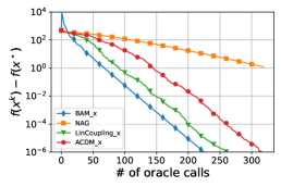
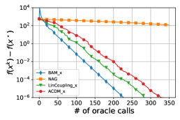
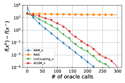
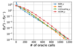
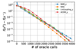
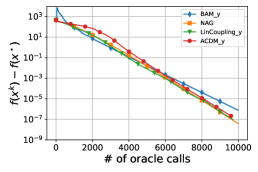
Figure 1: Comparison of Block Accelerated Method (BAM), Nesterov Accelerated Method (NAG), Accelerated Coordinate Descent Method (ACDM) and Linear Coupling method (LinCoupling) on quadratic functions. First line represents rate in terms of the $\nabla_{x}f(x,y)$ oracle calls and the second one represents rate in terms of the $\nabla_{y}f(x,y)$ oracle calls. We set $L_{y}=500$ (left column), $L_{y}=5000$ (middle column) and $L_{y}=50000$ (right column).

However, global model training can be prohibited in some settings even without sharing data due to privacy constraints. For example, using client-specific embeddings can reveal user identity, which is not allowed by a privacy policy. In order to fix this issue, a concept of partial federated learning was introduced (Singhal et al., 2021). In this approach, models have two blocks of parameters: global block $x$ and local blocks $y_{i}$, which never leave the clients. This technique enables to have interpolation between distributed and non-distributed learning. Partial federated learning is closely connected to personalizing and meta-learning algorithms. The most popular meta-learning algorithm is MAML (Finn et al., 2017), and connection to federated learning was established in several works (Nichol et al., 2018; Chen et al., 2018; Fallah et al., 2020).

5.2 Federated Reconstruction

Let us describe the baseline of partial federated learning called Federated Reconstruction. We have two blocks of coordinates in this framework: user-specific parameters $y_{i}$ and non-user-specific $x$ parameters. For every communication round, $t$ server sends the global part of parameters $x_{t}$ to all clients, and then each client reconstructs local parameters $y^{i}_{t}$ using the current global model $x_{t}$. The reconstruction process usually requires several steps. Once the local model is restored, each client updates its copy of global parameters and then sends only updated copies of the global model to the server. The server aggregates these updates and forms the next iterate $x_{t+1}$.

The new BAM algorithm can be generalized to minimize $f(x,y_{1},\ldots,y_{M})$ in a distributed setting, and this method can be applied to Federated Reconstruction. Since the communication complexity is proportional to the number of calls of $\nabla_{x}f(x,y_{1},\ldots,y_{M})$, the communication complexity is $\mathcal{O}\left(\sqrt{\frac{L_{x}}{\mu_{x}}}\log\frac{1}{\varepsilon}\right)$. The communication bottleneck can be overcome in case of a small condition number for local parameters. Moreover, this communication complexity will be optimal.

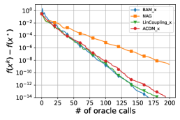
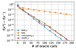
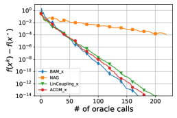
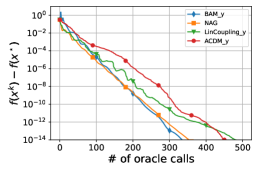
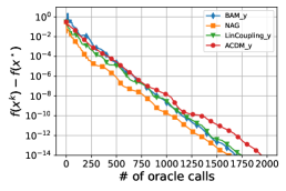
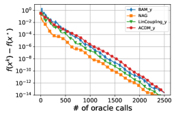
Figure 2: Comparison of Block Accelerated Method (BAM), Nesterov Accelerated Method (NAG), Accelerated Coordinate Descent Method (ACDM), and Linear Coupling method (LinCoupling) on logistic regression loss functions with two different $l_{2}$ regularizers. The first line represents the rate in terms of the $\nabla_{x}f(x,y)$ oracle calls, and the second one represents the rate in terms of the $\nabla_{y}f(x,y)$ oracle calls. We set $\mu_{y}=0.002$ (left column), $\mu_{y}=0.0001$ (middle column) and $\mu=0.00005$ (right column).

6 Experiments

In all our experiments, we compare the new Block Accelerated Method (BAM) with Nesterov Accelerated Method (NAG) (Nesterov, 1983), Accelerated Coordinate Descent Method (ACDM) (Nesterov & Stich, 2017) and Linear Coupling method (LinCoupling) (Allen-Zhu et al., 2016; Gasnikov et al., 2015).

6.1 Quadratic objectives

In our experiments, we first consider quadratic functions:

$$f(z)=z^{\top}Az+b^{\top}z,$$

where $z=(x,y)^{\top}$ is a joint vector of two blocks. The matrix spectrum is uniformly generated from $\mu_{x}$ to $L_{x}$ for the block $x$ of the matrix $A$ and from $\mu_{y}$ to $L_{y}$ for the block $y$ of matrix $A$. We set $\mu_{x}=\mu_{y}=0.1$, $L_{y}=50$ and we set dimensions of our blocks to be $d_{x}=100$ and $d_{y}=10$. We vary the parameter $L_{y}$ to obtain different condition numbers $\kappa_{y}$, and we consider $\nabla_{x}f(x,y)$ and $\nabla_{y}f(x,y)$ oracle calls to compare several methods.

6.2 Logistic regression

In our experiments, we also consider the logistic regression loss function with two $l_{2}$ regularizers for the click-prediction model:

$$f(x,y) :=\frac{1}{n}\sum_{k=1}^{n}\log\left(1+\exp\left(-\eta^{k}\langle\xi^{k},(x,y)\rangle\right)\right)$$

$$+\lambda_{x}\|x\|^{2}+\lambda_{y}\|y\|^{2}.$$

We used dataset ”a1a” from LIBSVM collection (Chang & Lin, 2011). The smoothness constant of this dataset is estimated as $L=1.567$. We set $d_{x}=100$, $d_{y}=19$ and $\mu_{x}=0.01$. We vary the parameter $\mu_{y}$ to obtain different condition numbers $\kappa_{y}$. We also consider two oracle calls of $\nabla_{x}f(x,y)$ and $\nabla_{y}f(x,y)$.

6.3 Results

In our experiments, as seen on plots, the new method shows better performance in terms of $\nabla_{x}f(x,y)$ oracle calls for both objective functions and all condition numbers. Moreover, all accelerated coordinate methods outperform Nesterov Gradient Method significantly, which confirms theoretical bounds. In terms of $\nabla_{y}f(x,y)$ oracle calls, the new method shows approximately the same results as other accelerated coordinate methods and Nesterov Gradient Method. In case of expensive $\nabla_{x}f(x,y)$ oracle calls, the new method can be useful. Moreover, the new method can be generalized to distributed and federated settings, which means that this method has practical perspectives.

7 Discussion

In this paper, we consider a convex optimization problem with a min-min structure

$$\min_{x,y}f(x,y).$$

Assuming that $f$ is $L$-smooth and $\mu_{x}$-strongly convex in $x$, $\mu_{y}$-strongly convex in $y$ we propose new Algorithm BAM that required $\mathcal{O}\left(\sqrt{L/\mu_{x}}\log\frac{1}{\epsilon}\right)$ calculations of $\nabla_{x}f$ and $\mathcal{O}\left(\sqrt{L/\mu_{y}}\log\frac{1}{\epsilon}\right)$ calculations of $\nabla_{y}f$. The proposed in the paper approach allows different generalizations. For example, it can be generalized to mixed oracles (Gladin et al., 2021b): e.g., instead of $\nabla_{y}f$, only the value of $f$ is available. Another generalization is increasing the number of blocks (in this paper, we consider only two blocks, $x$, and $y$) for clarity. BAM can also be joined with many other tricks. For example, it can be joined with composite sliding (Lan, 2016; Kovalev et al., 2022), described at the very beginning of the introduction.

Appendix A Supplementary materials

Proof of Lemma 2.1.

Using 1.1, we get

$$f(\overline{x}^{k+1},\overline{y}^{k+1}) \leq f(\underline{x}^{k},\overline{y}^{k+1})+\langle\nabla_{x}f(\underline{x}^{k},\overline{y}^{k+1}),\overline{x}^{k+1}-\underline{x}^{k}\rangle+\frac{L_{x}}{2}\|\overline{x}^{k+1}-\underline{x}^{k}\|^{2}$$

$$=f(\underline{x}^{k},\overline{y}^{k+1})+\eta_{x}\alpha\left(\frac{\eta_{x}\alpha L_{x}}{2}-1\right)\|\nabla_{x}f(\underline{x}^{k},\overline{y}^{k+1})\|^{2}$$

$$\leq f(\underline{x}^{k},\overline{y}^{k+1})+\eta_{x}\alpha\left(\frac{1}{2}-1\right)\|\nabla_{x}f(\underline{x}^{k},\overline{y}^{k+1})\|^{2}$$

$$\leq f(\underline{x}^{k},\overline{y}^{k+1})-\frac{\eta_{x}\alpha}{2}\|\nabla_{x}f(\underline{x}^{k},\overline{y}^{k+1})\|^{2}$$

∎

Proof of Theorem 2.2.

$$\eta_{x}^{-1}\mathcal{R}_{x}^{k+1}+\eta_{y}^{-1}\mathcal{R}_{y}^{k+1} =\eta_{x}^{-1}\mathcal{R}_{x}^{k}+\eta_{y}^{-1}\mathcal{R}_{y}^{k}-\eta_{x}^{-1}\|x^{k+1}-x^{k}\|^{2}-\eta_{y}^{-1}\|y^{k+1}-y^{k}\|^{2}$$

$$+2\eta_{x}^{-1}\langle x^{k+1}-x^{k},x^{k+1}-x^{*}\rangle+2\eta_{y}^{-1}\langle y^{k+1}-y^{k},y^{k+1}-y^{*}\rangle$$

$$=\eta_{x}^{-1}\mathcal{R}_{x}^{k}+\eta_{y}^{-1}\mathcal{R}_{y}^{k}-\eta_{x}^{-1}\|x^{k+1}-x^{k}\|^{2}-\eta_{y}^{-1}\|y^{k+1}-y^{k}\|^{2}$$

$$+2\eta_{x}^{-1}\alpha\langle\underline{x}_{k}-x^{k+1},x^{k+1}-x^{*}\rangle+2\eta_{y}^{-1}\langle\overline{y}^{k+1}-y^{k+1},y^{k+1}-y^{*}\rangle$$

$$-2\langle\nabla_{x}f(\underline{x}^{k},\overline{y}^{k+1}),x^{k+1}-x^{*}\rangle-2\langle\nabla_{y}f(\underline{x}^{k},\overline{y}^{k+1}),y^{k+1}-y^{*}\rangle$$

$$=\eta_{x}^{-1}\mathcal{R}_{x}^{k}+\eta_{y}^{-1}\mathcal{R}_{y}^{k}-\eta_{x}^{-1}\|x^{k+1}-x^{k}\|^{2}-\eta_{y}^{-1}\|y^{k+1}-y^{k}\|^{2}$$

$$+\eta_{x}^{-1}\alpha\left(\|\underline{x}^{k}-x^{*}\|^{2}-\|x^{k+1}-x^{*}\|^{2}-\|x^{k+1}-\underline{x}^{k}\|^{2}\right)$$

$$+\eta_{y}^{-1}\alpha\left(\|\overline{y}^{k+1}-y^{*}\|^{2}-\|y^{k+1}-y^{*}\|^{2}-\|y^{k+1}-\overline{y}^{k+1}\|^{2}\right)$$

$$-2\langle\nabla_{x}f(\underline{x}^{k},\overline{y}^{k+1}),x^{k+1}-x^{*}\rangle-2\langle\nabla_{y}f(\underline{x}^{k},\overline{y}^{k+1}),y^{k+1}-y^{*}\rangle$$

$$\leq\eta_{x}^{-1}\mathcal{R}_{x}^{k}+\eta_{y}^{-1}\mathcal{R}_{y}^{k}-\eta_{x}^{-1}\|x^{k+1}-x^{k}\|^{2}-\eta_{y}^{-1}\|y^{k+1}-y^{k}\|^{2}$$

$$+\eta_{x}^{-1}\alpha\left(\|\underline{x}^{k}-x^{*}\|^{2}-\|x^{k+1}-x^{*}\|^{2}\right)$$

$$+\eta_{y}^{-1}\alpha\left(\|\overline{y}^{k+1}-y^{*}\|^{2}-\|y^{k+1}-y^{*}\|^{2}\right)$$

$$-2\langle\nabla_{x}f(\underline{x}^{k},\overline{y}^{k+1}),x^{k+1}-x^{*}\rangle-2\langle\nabla_{y}f(\underline{x}^{k},\overline{y}^{k+1}),y^{k+1}-y^{*}\rangle.$$

This implies

$$(1+\alpha)\left(\eta_{x}^{-1}\mathcal{R}_{x}^{k+1}+\eta_{y}^{-1}\mathcal{R}_{y}^{k+1}\right) \leq\eta_{x}^{-1}\mathcal{R}_{x}^{k}+\eta_{y}^{-1}\mathcal{R}_{y}^{k}-\eta_{x}^{-1}\|x^{k+1}-x^{k}\|^{2}-\eta_{y}^{-1}\|y^{k+1}-y^{k}\|^{2}$$

$$+\eta_{x}^{-1}\alpha\|\underline{x}^{k}-x^{*}\|^{2}+\eta_{y}^{-1}\alpha\|\overline{y}^{k+1}-y^{*}\|^{2}$$

$$-2\langle\nabla_{x}f(\underline{x}^{k},\overline{y}^{k+1}),x^{k+1}-x^{*}\rangle-2\langle\nabla_{y}f(\underline{x}^{k},\overline{y}^{k+1}),y^{k+1}-y^{*}\rangle$$

$$=\eta_{x}^{-1}\mathcal{R}_{x}^{k}+\eta_{y}^{-1}\mathcal{R}_{y}^{k}-\eta_{x}^{-1}\|x^{k+1}-x^{k}\|^{2}-\eta_{y}^{-1}\|y^{k+1}-y^{k}\|^{2}$$

$$+\eta_{x}^{-1}\alpha\|\underline{x}^{k}-x^{*}\|^{2}+\eta_{y}^{-1}\alpha\|\overline{y}^{k+1}-y^{*}\|^{2}$$

$$-2\langle\nabla_{x}f(\underline{x}^{k},\overline{y}^{k+1}),x^{k+1}-x^{k}\rangle-2\langle\nabla_{x}f(\underline{x}^{k},\overline{y}^{k+1}),x^{k}-x^{*}\rangle$$

$$-2\langle\nabla_{y}f(\underline{x}^{k},\overline{y}^{k+1}),y^{k+1}-y^{k}\rangle-2\langle\nabla_{y}f(\underline{x}^{k},\overline{y}^{k+1}),y^{k}-y^{*}\rangle.$$

Using Young’s inequality, we get

$$(1+\alpha)\left(\eta_{x}^{-1}\mathcal{R}_{x}^{k+1}+\eta_{y}^{-1}\mathcal{R}_{y}^{k+1}\right) \leq\eta_{x}^{-1}\mathcal{R}_{x}^{k}+\eta_{y}^{-1}\mathcal{R}_{y}^{k}-\eta_{x}^{-1}\|x^{k+1}-x^{k}\|^{2}-\eta_{y}^{-1}\|y^{k+1}-y^{k}\|^{2}$$

$$+\eta_{x}^{-1}\alpha\|\underline{x}^{k}-x^{*}\|^{2}+\eta_{y}^{-1}\alpha\|\overline{y}^{k+1}-y^{*}\|^{2}$$

$$+\eta_{x}^{-1}\|x^{k+1}-x^{k}\|^{2}+\eta_{x}\|\nabla_{x}f(\underline{x}^{k},\overline{y}^{k+1})\|^{2}-2\langle\nabla_{x}f(\underline{x}^{k},\overline{y}^{k+1}),x^{k}-x^{*}\rangle$$

$$+\eta_{y}^{-1}\|y^{k+1}-y^{k}\|^{2}+\eta_{y}\|\nabla_{y}f(\underline{x}^{k},\overline{y}^{k+1})\|^{2}-2\langle\nabla_{y}f(\underline{x}^{k},\overline{y}^{k+1}),y^{k}-y^{*}\rangle$$

$$=\eta_{x}^{-1}\mathcal{R}_{x}^{k}+\eta_{y}^{-1}\mathcal{R}_{y}^{k}+\eta_{x}^{-1}\alpha\|\underline{x}^{k}-x^{*}\|^{2}+\eta_{y}^{-1}\alpha\|\overline{y}^{k+1}-y^{*}\|^{2}$$

$$+\eta_{x}\|\nabla_{x}f(\underline{x}^{k},\overline{y}^{k+1})\|^{2}+\eta_{y}\|\nabla_{y}f(\underline{x}^{k},\overline{y}^{k+1})\|^{2}$$

$$-2\langle\nabla_{x}f(\underline{x}^{k},\overline{y}^{k+1}),x^{k}-x^{*}\rangle-2\langle\nabla_{y}f(\underline{x}^{k},\overline{y}^{k+1}),y^{k}-y^{*}\rangle$$

$$=\eta_{x}^{-1}\mathcal{R}_{x}^{k}+\eta_{y}^{-1}\mathcal{R}_{y}^{k}+\eta_{x}^{-1}\alpha\|\underline{x}^{k}-x^{*}\|^{2}+\eta_{y}^{-1}\alpha\|\overline{y}^{k+1}-y^{*}\|^{2}$$

$$+\eta_{x}\|\nabla_{x}f(\underline{x}^{k},\overline{y}^{k+1})\|^{2}+\eta_{y}\|\nabla_{y}f(\underline{x}^{k},\overline{y}^{k+1})\|^{2}$$

$$-2\langle\nabla_{x}f(\underline{x}^{k},\overline{y}^{k+1}),\underline{x}^{k}-x^{*}\rangle-2\langle\nabla_{y}f(\underline{x}^{k},\overline{y}^{k+1}),\overline{y}^{k+1}-y^{*}\rangle$$

$$-2\langle\nabla_{x}f(\underline{x}^{k},\overline{y}^{k+1}),x^{k}-\underline{x}^{k}\rangle-2\langle\nabla_{y}f(\underline{x}^{k},\overline{y}^{k+1}),y^{k}-\overline{y}^{k+1}\rangle$$

Using 1.2, we get

$$(1+\alpha)\left(\eta_{x}^{-1}\mathcal{R}_{x}^{k+1}+\eta_{y}^{-1}\mathcal{R}_{y}^{k+1}\right) \leq\eta_{x}^{-1}\mathcal{R}_{x}^{k}+\eta_{y}^{-1}\mathcal{R}_{y}^{k}+\eta_{x}^{-1}\alpha\|\underline{x}^{k}-x^{*}\|^{2}+\eta_{y}^{-1}\alpha\|\overline{y}^{k+1}-y^{*}\|^{2}$$

$$+\eta_{x}\|\nabla_{x}f(\underline{x}^{k},\overline{y}^{k+1})\|^{2}+\eta_{y}\|\nabla_{y}f(\underline{x}^{k},\overline{y}^{k+1})\|^{2}$$

$$+2\left(f(x^{*},y^{*})-f(\underline{x}^{k},\overline{y}^{k+1})\right)-\mu_{x}\|\underline{x}^{k}-x^{*}\|^{2}-\mu_{y}\|\overline{y}^{k+1}-y^{*}\|^{2}$$

$$-2\langle\nabla_{x}f(\underline{x}^{k},\overline{y}^{k+1}),x^{k}-\underline{x}^{k}\rangle-2\langle\nabla_{y}f(\underline{x}^{k},\overline{y}^{k+1}),y^{k}-\overline{y}^{k+1}\rangle$$

$$=\eta_{x}^{-1}\mathcal{R}_{x}^{k}+\eta_{y}^{-1}\mathcal{R}_{y}^{k}+(\eta_{x}^{-1}\alpha-\mu_{x})\|\underline{x}^{k}-x^{*}\|^{2}+(\eta_{y}^{-1}\alpha-\mu_{y})\|\overline{y}^{k+1}-y^{*}\|^{2}$$

$$+\eta_{x}\|\nabla_{x}f(\underline{x}^{k},\overline{y}^{k+1})\|^{2}+\eta_{y}\|\nabla_{y}f(\underline{x}^{k},\overline{y}^{k+1})\|^{2}+2\left(f(x^{*},y^{*})-f(\underline{x}^{k},\overline{y}^{k+1})\right)$$

$$-2\langle\nabla_{x}f(\underline{x}^{k},\overline{y}^{k+1}),x^{k}-\underline{x}^{k}\rangle-2\langle\nabla_{y}f(\underline{x}^{k},\overline{y}^{k+1}),y^{k}-\overline{y}^{k+1}\rangle$$

$$=\eta_{x}^{-1}\mathcal{R}_{x}^{k}+\eta_{y}^{-1}\mathcal{R}_{y}^{k}+(\eta_{x}^{-1}\alpha-\mu_{x})\|\underline{x}^{k}-x^{*}\|^{2}+(\eta_{y}^{-1}\alpha-\mu_{y})\|\overline{y}^{k+1}-y^{*}\|^{2}$$

$$+\eta_{x}\|\nabla_{x}f(\underline{x}^{k},\overline{y}^{k+1})\|^{2}+\eta_{y}\|\nabla_{y}f(\underline{x}^{k},\overline{y}^{k+1})\|^{2}+2\left(f(x^{*},y^{*})-f(\underline{x}^{k},\overline{y}^{k+1})\right)$$

$$+\frac{2(1-\alpha)}{\alpha}\langle\nabla_{x}f(\underline{x}^{k},\overline{y}^{k+1}),\overline{x}^{k}-\underline{x}^{k}\rangle$$

$$-\langle\nabla_{y}f(\underline{x}^{k},\overline{y}^{k+1}),\frac{2}{\alpha}(\underline{y}^{k}-(1-\alpha)\overline{y}^{k})-\overline{y}^{k+1}\rangle$$

$$=\eta_{x}^{-1}\mathcal{R}_{x}^{k}+\eta_{y}^{-1}\mathcal{R}_{y}^{k}+(\eta_{x}^{-1}\alpha-\mu_{x})\|\underline{x}^{k}-x^{*}\|^{2}+(\eta_{y}^{-1}\alpha-\mu_{y})\|\overline{y}^{k+1}-y^{*}\|^{2}$$

$$+\eta_{x}\|\nabla_{x}f(\underline{x}^{k},\overline{y}^{k+1})\|^{2}+\eta_{y}\|\nabla_{y}f(\underline{x}^{k},\overline{y}^{k+1})\|^{2}+2\left(f(x^{*},y^{*})-f(\underline{x}^{k},\overline{y}^{k+1})\right)$$

$$+\frac{2(1-\alpha)}{\alpha}\langle\nabla_{x}f(\underline{x}^{k},\overline{y}^{k+1}),\overline{x}^{k}-\underline{x}^{k}\rangle$$

$$+\frac{2}{\alpha}\langle\nabla_{y}f(\underline{x}^{k},\overline{y}^{k+1}),\overline{y}^{k+1}-\underline{y}^{k}+(1-\alpha)\overline{y}^{k}-(1-\alpha)\overline{y}^{k+1}\rangle$$

$$=\eta_{x}^{-1}\mathcal{R}_{x}^{k}+\eta_{y}^{-1}\mathcal{R}_{y}^{k}+(\eta_{x}^{-1}\alpha-\mu_{x})\|\underline{x}^{k}-x^{*}\|^{2}+(\eta_{y}^{-1}\alpha-\mu_{y})\|\overline{y}^{k+1}-y^{*}\|^{2}$$

$$+\eta_{x}\|\nabla_{x}f(\underline{x}^{k},\overline{y}^{k+1})\|^{2}+\eta_{y}\|\nabla_{y}f(\underline{x}^{k},\overline{y}^{k+1})\|^{2}+2\left(f(x^{*},y^{*})-f(\underline{x}^{k},\overline{y}^{k+1})\right)$$

$$+\frac{2(1-\alpha)}{\alpha}\left(\langle\nabla_{x}f(\underline{x}^{k},\overline{y}^{k+1}),\overline{x}^{k}-\underline{x}^{k}\rangle+\langle\nabla_{y}f(\underline{x}^{k},\overline{y}^{k+1}),\overline{y}^{k}-\overline{y}^{k+1}\rangle\right)$$

$$+\frac{2}{\alpha}\langle\nabla_{y}f(\underline{x}^{k},\overline{y}^{k+1}),\overline{y}^{k+1}-\underline{y}^{k}\rangle.$$

Using convexity of $f(x,y)$, we get

$$(1+\alpha)\left(\eta_{x}^{-1}\mathcal{R}_{x}^{k+1}+\eta_{y}^{-1}\mathcal{R}_{y}^{k+1}\right) \leq\eta_{x}^{-1}\mathcal{R}_{x}^{k}+\eta_{y}^{-1}\mathcal{R}_{y}^{k}+(\eta_{x}^{-1}\alpha-\mu_{x})\|\underline{x}^{k}-x^{*}\|^{2}+(\eta_{y}^{-1}\alpha-\mu_{y})\|\overline{y}^{k+1}-y^{*}\|^{2}$$

$$+\eta_{x}\|\nabla_{x}f(\underline{x}^{k},\overline{y}^{k+1})\|^{2}+\eta_{y}\|\nabla_{y}f(\underline{x}^{k},\overline{y}^{k+1})\|^{2}+2\left(f(x^{*},y^{*})-f(\underline{x}^{k},\overline{y}^{k+1})\right)$$

$$+\frac{2(1-\alpha)}{\alpha}\left(f(\overline{x}^{k},\overline{y}^{k})-f(\underline{x}^{k},\overline{y}^{k+1})\right)+\frac{2}{\alpha}\langle\nabla_{y}f(\underline{x}^{k},\overline{y}^{k+1}),\overline{y}^{k+1}-\underline{y}^{k}\rangle.$$

$$=\eta_{x}^{-1}\mathcal{R}_{x}^{k}+\eta_{y}^{-1}\mathcal{R}_{y}^{k}+(\eta_{x}^{-1}\alpha-\mu_{x})\|\underline{x}^{k}-x^{*}\|^{2}+(\eta_{y}^{-1}\alpha-\mu_{y})\|\overline{y}^{k+1}-y^{*}\|^{2}$$

$$+\eta_{x}\|\nabla_{x}f(\underline{x}^{k},\overline{y}^{k+1})\|^{2}+\eta_{y}\|\nabla_{y}f(\underline{x}^{k},\overline{y}^{k+1})\|^{2}$$

$$+2f(x^{*},y^{*})+\frac{2(1-\alpha)}{\alpha}f(\overline{x}^{k},\overline{y}^{k})-\frac{2}{\alpha}f(\underline{x}^{k},\overline{y}^{k+1})$$

$$+\frac{2}{\alpha}\langle\nabla_{y}f(\underline{x}^{k},\overline{y}^{k+1}),\overline{y}^{k+1}-\underline{y}^{k}\rangle.$$

Using Lemma 2.1, we get

$$(1+\alpha)\left(\eta_{x}^{-1}\mathcal{R}_{x}^{k+1}+\eta_{y}^{-1}\mathcal{R}_{y}^{k+1}\right) \leq\eta_{x}^{-1}\mathcal{R}_{x}^{k}+\eta_{y}^{-1}\mathcal{R}_{y}^{k}+(\eta_{x}^{-1}\alpha-\mu_{x})\|\underline{x}^{k}-x^{*}\|^{2}+(\eta_{y}^{-1}\alpha-\mu_{y})\|\overline{y}^{k+1}-y^{*}\|^{2}$$

$$+\eta_{x}\|\nabla_{x}f(\underline{x}^{k},\overline{y}^{k+1})\|^{2}+\eta_{y}\|\nabla_{y}f(\underline{x}^{k},\overline{y}^{k+1})\|^{2}$$

$$+2f(x^{*},y^{*})+\frac{2(1-\alpha)}{\alpha}f(\overline{x}^{k},\overline{y}^{k})$$

$$-\frac{2}{\alpha}\left(f(\overline{x}^{k+1},\overline{y}^{k+1})+\frac{\eta_{x}\alpha}{2}\|\nabla_{x}f(\underline{x}^{k},\overline{y}^{k+1})\|^{2}\right)$$

$$+\frac{2}{\alpha}\langle\nabla_{y}f(\underline{x}^{k},\overline{y}^{k+1}),\overline{y}^{k+1}-\underline{y}^{k}\rangle$$

$$=\eta_{x}^{-1}\mathcal{R}_{x}^{k}+\eta_{y}^{-1}\mathcal{R}_{y}^{k}+(\eta_{x}^{-1}\alpha-\mu_{x})\|\underline{x}^{k}-x^{*}\|^{2}+(\eta_{y}^{-1}\alpha-\mu_{y})\|\overline{y}^{k+1}-y^{*}\|^{2}$$

$$+\frac{2(1-\alpha)}{\alpha}\left(f(\overline{x}^{k},\overline{y}^{k})-f(x^{*},y^{*})\right)-\frac{2}{\alpha}\left(f(\overline{x}^{k+1},\overline{y}^{k+1})-f(x^{*},y^{*})\right)$$

$$+\eta_{y}\|\nabla_{y}f(\underline{x}^{k},\overline{y}^{k+1})\|^{2}+\frac{2}{\alpha}\langle\nabla_{y}f(\underline{x}^{k},\overline{y}^{k+1}),\overline{y}^{k+1}-\underline{y}^{k}\rangle$$

$$=\eta_{x}^{-1}\mathcal{R}_{x}^{k}+\eta_{y}^{-1}\mathcal{R}_{y}^{k}+(\eta_{x}^{-1}\alpha-\mu_{x})\|\underline{x}^{k}-x^{*}\|^{2}+(\eta_{y}^{-1}\alpha-\mu_{y})\|\overline{y}^{k+1}-y^{*}\|^{2}$$

$$+\frac{2(1-\alpha)}{\alpha}\left(f(\overline{x}^{k},\overline{y}^{k})-f(x^{*},y^{*})\right)-\frac{2}{\alpha}\left(f(\overline{x}^{k+1},\overline{y}^{k+1})-f(x^{*},y^{*})\right)$$

$$+\eta_{y}\|\nabla_{y}f(\underline{x}^{k},\overline{y}^{k+1})\|^{2}+2\eta_{y}\langle\nabla_{y}f(\underline{x}^{k},\overline{y}^{k+1}),(\eta_{y}\alpha)^{-1}(\overline{y}^{k+1}-\underline{y}^{k})\rangle$$

$$=\eta_{x}^{-1}\mathcal{R}_{x}^{k}+\eta_{y}^{-1}\mathcal{R}_{y}^{k}+(\eta_{x}^{-1}\alpha-\mu_{x})\|\underline{x}^{k}-x^{*}\|^{2}+(\eta_{y}^{-1}\alpha-\mu_{y})\|\overline{y}^{k+1}-y^{*}\|^{2}$$

$$+\frac{2(1-\alpha)}{\alpha}\left(f(\overline{x}^{k},\overline{y}^{k})-f(x^{*},y^{*})\right)-\frac{2}{\alpha}\left(f(\overline{x}^{k+1},\overline{y}^{k+1})-f(x^{*},y^{*})\right)$$

$$+\eta_{y}\|\nabla_{y}f(\underline{x}^{k},\overline{y}^{k+1})\|^{2}+\eta_{y}\|\nabla_{y}f(\underline{x}^{k},\overline{y}^{k+1})+(\eta_{y}\alpha)^{-1}(\overline{y}^{k+1}-\underline{y}^{k})\|^{2}$$

$$-\eta_{y}\|\nabla_{y}f(\underline{x}^{k},\overline{y}^{k+1})\|^{2}-\eta_{y}^{-1}\alpha^{-2}\|\overline{y}^{k+1}-\underline{y}^{k}\|^{2}$$

$$=\eta_{x}^{-1}\mathcal{R}_{x}^{k}+\eta_{y}^{-1}\mathcal{R}_{y}^{k}+(\eta_{x}^{-1}\alpha-\mu_{x})\|\underline{x}^{k}-x^{*}\|^{2}+(\eta_{y}^{-1}\alpha-\mu_{y})\|\overline{y}^{k+1}-y^{*}\|^{2}$$

$$+\frac{2(1-\alpha)}{\alpha}\left(f(\overline{x}^{k},\overline{y}^{k})-f(x^{*},y^{*})\right)-\frac{2}{\alpha}\left(f(\overline{x}^{k+1},\overline{y}^{k+1})-f(x^{*},y^{*})\right)$$

$$+\eta_{y}\left(\|\nabla_{y}f(\underline{x}^{k},\overline{y}^{k+1})+(\eta_{y}\alpha)^{-1}(\overline{y}^{k+1}-\underline{y}^{k})\|^{2}-(\eta_{y}\alpha)^{-2}\|\overline{y}^{k+1}-\underline{y}^{k}\|^{2}\right).$$

Using inequality (5), we get

$$(1+\alpha)\left(\eta_{x}^{-1}\mathcal{R}_{x}^{k+1}+\eta_{y}^{-1}\mathcal{R}_{y}^{k+1}\right) \leq\eta_{x}^{-1}\mathcal{R}_{x}^{k}+\eta_{y}^{-1}\mathcal{R}_{y}^{k}+(\eta_{x}^{-1}\alpha-\mu_{x})\|\underline{x}^{k}-x^{*}\|^{2}+(\eta_{y}^{-1}\alpha-\mu_{y})\|\overline{y}^{k+1}-y^{*}\|^{2}$$

$$+\frac{2(1-\alpha)}{\alpha}\left(f(\overline{x}^{k},\overline{y}^{k})-f(x^{*},y^{*})\right)-\frac{2}{\alpha}\left(f(\overline{x}^{k+1},\overline{y}^{k+1})-f(x^{*},y^{*})\right).$$

Using the choice of parameters $\eta_{x},\eta_{y},\alpha$, we get

$$(1+\alpha)\left(\eta_{x}^{-1}\mathcal{R}_{x}^{k+1}+\eta_{y}^{-1}\mathcal{R}_{y}^{k+1}\right) \leq\eta_{x}^{-1}\mathcal{R}_{x}^{k}+\eta_{y}^{-1}\mathcal{R}_{y}^{k}+\frac{2(1-\alpha)}{\alpha}\left(f(\overline{x}^{k},\overline{y}^{k})-f(x^{*},y^{*})\right)$$

$$-\frac{2}{\alpha}\left(f(\overline{x}^{k+1},\overline{y}^{k+1})-f(x^{*},y^{*})\right).$$

After rearranging, we get

$$\Psi^{k+1} \leq\eta_{x}^{-1}\mathcal{R}_{x}^{k}+\eta_{y}^{-1}\mathcal{R}_{y}^{k}+\frac{2(1-\alpha)}{\alpha}\left(f(\overline{x}^{k},\overline{y}^{k})-f(x^{*},y^{*})\right)$$

$$\leq\eta_{x}^{-1}\mathcal{R}_{x}^{k}+\eta_{y}^{-1}\mathcal{R}_{y}^{k}+\frac{2(1+\alpha)^{-1}}{\alpha}\left(f(\overline{x}^{k},\overline{y}^{k})-f(x^{*},y^{*})\right)$$

$$=(1+\alpha)^{-1}\Psi^{k}.$$

∎

Proof of Corollary 3.2.

Using inequality (13) and (14), we get

$$\|\nabla A^{k}(\overline{y}^{k+1})\| \leq\frac{(\eta_{y}\alpha)^{-1}}{2}\|\underline{y}^{k}-\operatorname*{arg\,min}_{y\in\mathbb{R}^{d_{y}}}A^{k}(y)\|$$

$$\leq\frac{(\eta_{y}\alpha)^{-1}}{2}\|\overline{y}^{k+1}-\underline{y}^{k}\|+\frac{(\eta_{y}\alpha)^{-1}}{2}\|\overline{y}^{k+1}-\operatorname*{arg\,min}_{y\in\mathbb{R}^{d_{y}}}A^{k}(y)\|.$$

Function $A^{k}(y)$ is $(\eta_{y}\alpha)^{-1}$-strongly convex which implies

$$(\eta_{y}\alpha)^{-1}\|\overline{y}^{k+1}-\operatorname*{arg\,min}_{y\in\mathbb{R}^{d_{y}}}A^{k}(y)\|\leq\|\nabla A^{k}(\overline{y}^{k+1})-\nabla A^{k}(\operatorname*{arg\,min}_{y\in\mathbb{R}^{d_{y}}}A^{k}(y))\|=\|\nabla A^{k}(\overline{y}^{k+1})\|.$$ (17)

Hence,

$$\|\nabla A^{k}(\overline{y}^{k+1})\| \leq\frac{(\eta_{y}\alpha)^{-1}}{2}\|\overline{y}^{k+1}-\underline{y}^{k}\|+\frac{1}{2}\|\nabla A^{k}(\overline{y}^{k+1})\|.$$

Rearranging concludes the proof. ∎

References

• Allen-Zhu et al. (2016) Allen-Zhu, Z., Qu, Z., Richtárik, P., and Yuan, Y. Even faster accelerated coordinate descent using non-uniform sampling. In International Conference on Machine Learning, pp. 1110–1119. PMLR, 2016.
• Beck (2017) Beck, A. First-order methods in optimization. SIAM, 2017.
• Bolte et al. (2020) Bolte, J., Glaudin, L., Pauwels, E., and Serrurier, M. Ah$\backslash$” olderian backtracking method for min-max and min-min problems. arXiv preprint arXiv:2007.08810, 2020.
• Carmon et al. (2022) Carmon, Y., Jambulapati, A., Jin, Y., and Sidford, A. Recapp: Crafting a more efficient catalyst for convex optimization. In International Conference on Machine Learning, pp. 2658–2685. PMLR, 2022.
• Chang & Lin (2011) Chang, C.-C. and Lin, C.-J. LIBSVM: A library for support vector machines. ACM Transactions on Intelligent Systems and Technology, 2:27:1–27:27, 2011. Software available at http://www.csie.ntu.edu.tw/~cjlin/libsvm.
• Chen et al. (2018) Chen, F., Luo, M., Dong, Z., Li, Z., and He, X. Federated meta-learning with fast convergence and efficient communication. arXiv preprint arXiv:1802.07876, 2018.
• Condat et al. (2022) Condat, L., Agarsky, I., and Richtárik, P. Provably doubly accelerated federated learning: The first theoretically successful combination of local training and compressed communication. arXiv preprint arXiv:2210.13277, 2022.
• De Cea et al. (2005) De Cea, J., Fernández, J. E., Dekock, V., and Soto, A. Solving network equilibrium problems on multimodal urban transportation networks with multiple user classes. Transport Reviews, 25(3):293–317, 2005.
• Diakonikolas & Orecchia (2018) Diakonikolas, J. and Orecchia, L. Alternating randomized block coordinate descent. In International Conference on Machine Learning, pp. 1224–1232. PMLR, 2018.
• Diakonikolas & Wang (2022) Diakonikolas, J. and Wang, P. Potential function-based framework for minimizing gradients in convex and min-max optimization. SIAM Journal on Optimization, 32(3):1668–1697, 2022.
• Dvurechensky et al. (2022) Dvurechensky, P., Kamzolov, D., Lukashevich, A., Lee, S., Ordentlich, E., Uribe, C. A., and Gasnikov, A. Hyperfast second-order local solvers for efficient statistically preconditioned distributed optimization. EURO Journal on Computational Optimization, 10:100045, 2022.
• Fallah et al. (2020) Fallah, A., Mokhtari, A., and Ozdaglar, A. Personalized federated learning: A meta-learning approach. arXiv preprint arXiv:2002.07948, 2020.
• Finn et al. (2017) Finn, C., Abbeel, P., and Levine, S. Model-agnostic meta-learning for fast adaptation of deep networks. In International conference on machine learning, pp. 1126–1135. PMLR, 2017.
• Gasnikov et al. (2015) Gasnikov, A., Dvurechensky, P., and Usmanova, I. About accelerated randomized methods. arXiv preprint arXiv:1508.02182, 2015.
• Gasnikov et al. (2014) Gasnikov, A. V., Dorn, Y. V., Nesterov, Y. E., and Shpirko, S. V. On the three-stage version of stable dynamic model. Matematicheskoe modelirovanie, 26(6):34–70, 2014.
• Gasnikov et al. (2016) Gasnikov, A. V., Gasnikova, E., Nesterov, Y. E., and Chernov, A. Efficient numerical methods for entropy-linear programming problems. Computational Mathematics and Mathematical Physics, 56(4):514–524, 2016.
• Gasnikov et al. (2021) Gasnikov, A. V., Dvinskikh, D. M., Dvurechensky, P., Kamzolov, D., Matyukhin, V. V., Pasechnyuk, D. A., Tupitsa, N. K., and Chernov, A. V. Accelerated meta-algorithm for convex optimization problems. Computational Mathematics and Mathematical Physics, 61(1):17–28, 2021.
• Gladin et al. (2021a) Gladin, E., Alkousa, M., and Gasnikov, A. Solving convex min-min problems with smoothness and strong convexity in one group of variables and low dimension in the other. Automation and Remote Control, 82(10):1679–1691, 2021a.
• Gladin et al. (2021b) Gladin, E., Sadiev, A., Gasnikov, A., Dvurechensky, P., Beznosikov, A., and Alkousa, M. Solving smooth min-min and min-max problems by mixed oracle algorithms. In International Conference on Mathematical Optimization Theory and Operations Research, pp.  19–40. Springer, 2021b.
• Gorbunov et al. (2021) Gorbunov, E., Hanzely, F., and Richtárik, P. Local sgd: Unified theory and new efficient methods. In International Conference on Artificial Intelligence and Statistics, pp.  3556–3564. PMLR, 2021.
• Grudzień et al. (2022) Grudzień, M., Malinovsky, G., and Richtárik, P. Can 5th generation local training methods support client sampling? yes! arXiv preprint arXiv:2212.14370, 2022.
• Guminov et al. (2021) Guminov, S., Dvurechensky, P., Tupitsa, N., and Gasnikov, A. On a combination of alternating minimization and nesterov’s momentum. In International Conference on Machine Learning, pp. 3886–3898. PMLR, 2021.
• Hard et al. (2018) Hard, A., Rao, K., Mathews, R., Ramaswamy, S., Beaufays, F., Augenstein, S., Eichner, H., Kiddon, C., and Ramage, D. Federated learning for mobile keyboard prediction. arXiv preprint arXiv:1811.03604, 2018.
• Ivanova et al. (2021) Ivanova, A., Pasechnyuk, D., Grishchenko, D., Shulgin, E., Gasnikov, A., and Matyukhin, V. Adaptive catalyst for smooth convex optimization. In International Conference on Optimization and Applications, pp.  20–37. Springer, 2021.
• Ivanova et al. (2022) Ivanova, A., Dvurechensky, P., Vorontsova, E., Pasechnyuk, D., Gasnikov, A., Dvinskikh, D., and Tyurin, A. Oracle complexity separation in convex optimization. Journal of Optimization Theory and Applications, 193(1):462–490, 2022.
• Karimireddy et al. (2020) Karimireddy, S. P., Kale, S., Mohri, M., Reddi, S., Stich, S., and Suresh, A. T. Scaffold: Stochastic controlled averaging for federated learning. In International Conference on Machine Learning, pp. 5132–5143. PMLR, 2020.
• Khaled et al. (2020) Khaled, A., Mishchenko, K., and Richtárik, P. Tighter theory for local sgd on identical and heterogeneous data. In International Conference on Artificial Intelligence and Statistics, pp.  4519–4529. PMLR, 2020.
• Kim & Fessler (2021) Kim, D. and Fessler, J. A. Optimizing the efficiency of first-order methods for decreasing the gradient of smooth convex functions. Journal of optimization theory and applications, 188(1):192–219, 2021.
• Koloskova et al. (2020) Koloskova, A., Loizou, N., Boreiri, S., Jaggi, M., and Stich, S. A unified theory of decentralized sgd with changing topology and local updates. In International Conference on Machine Learning, pp. 5381–5393. PMLR, 2020.
• Konečnỳ et al. (2016) Konečnỳ, J., McMahan, H. B., Yu, F. X., Richtárik, P., Suresh, A. T., and Bacon, D. Federated learning: Strategies for improving communication efficiency. arXiv preprint arXiv:1610.05492, 2016.
• Kovalev & Gasnikov (2022a) Kovalev, D. and Gasnikov, A. The first optimal algorithm for smooth and strongly-convex-strongly-concave minimax optimization. In Advances in Neural Information Processing Systems, 2022a.
• Kovalev & Gasnikov (2022b) Kovalev, D. and Gasnikov, A. The first optimal acceleration of high-order methods in smooth convex optimization. In Advances in Neural Information Processing Systems, 2022b.
• Kovalev et al. (2022) Kovalev, D., Beznosikov, A., Borodich, E. D., Gasnikov, A., and Scutari, G. Optimal gradient sliding and its application to optimal distributed optimization under similarity. In Advances in Neural Information Processing Systems, 2022.
• Lan (2016) Lan, G. Gradient sliding for composite optimization. Mathematical Programming, 159(1):201–235, 2016.
• Malinovsky et al. (2022) Malinovsky, G., Yi, K., and Richtárik, P. Variance reduced proxskip: Algorithm, theory and application to federated learning. arXiv preprint arXiv:2207.04338, 2022.
• McMahan et al. (2017) McMahan, B., Moore, E., Ramage, D., Hampson, S., and y Arcas, B. A. Communication-efficient learning of deep networks from decentralized data. In Artificial intelligence and statistics, pp.  1273–1282. PMLR, 2017.
• Mishchenko et al. (2022) Mishchenko, K., Malinovsky, G., Stich, S., and Richtárik, P. Proxskip: Yes! local gradient steps provably lead to communication acceleration! finally! In International Conference on Machine Learning, pp. 15750–15769. PMLR, 2022.
• Mitra et al. (2021) Mitra, A., Jaafar, R., Pappas, G. J., and Hassani, H. Linear convergence in federated learning: Tackling client heterogeneity and sparse gradients. Advances in Neural Information Processing Systems, 34:14606–14619, 2021.
• Nemirovski & Yudin (1983) Nemirovski, A. and Yudin, D. Problem complexity and method efficiency in Optimization. J. Wiley & Sons, 1983.
• Nesterov (2012) Nesterov, Y. Efficiency of coordinate descent methods on huge-scale optimization problems. SIAM Journal on Optimization, 22(2):341–362, 2012.
• Nesterov (2018) Nesterov, Y. Lectures on convex optimization, volume 137. Springer, 2018.
• Nesterov (2020) Nesterov, Y. Soft clustering by convex electoral model. Soft Computing, 24(23):17609–17620, 2020.
• Nesterov (May 14, 2015) Nesterov, Y. Structural optimization: New perspectives for increasing efficiency of numerical schemes. nternational conference ”Optimization and Applications in Control and Data Science” on the occasion of Boris Polyak’s 80th birthday, May 14, 2015. URL https://www.mathnet.ru/php/presentation.phtml?option_lang=rus&presentid=11909.
• Nesterov & Stich (2017) Nesterov, Y. and Stich, S. U. Efficiency of the accelerated coordinate descent method on structured optimization problems. SIAM Journal on Optimization, 27(1):110–123, 2017.
• Nesterov et al. (2021) Nesterov, Y., Gasnikov, A., Guminov, S., and Dvurechensky, P. Primal–dual accelerated gradient methods with small-dimensional relaxation oracle. Optimization Methods and Software, 36(4):773–810, 2021.
• Nesterov (1983) Nesterov, Y. E. A method of solving a convex programming problem with convergence rate $\mathcal{O}(1/k^{2})$. In Doklady Akademii Nauk, volume 269, pp.  543–547. Russian Academy of Sciences, 1983.
• Nichol et al. (2018) Nichol, A., Achiam, J., and Schulman, J. On first-order meta-learning algorithms. arXiv preprint arXiv:1803.02999, 2018.
• Ostroukhov (2022) Ostroukhov, P. A. Tensor methods inside mixed oracle for min-min problems. Computer Research and Modeling, 14(2):377–398, 2022.
• Richtárik & Takáč (2014) Richtárik, P. and Takáč, M. Iteration complexity of randomized block-coordinate descent methods for minimizing a composite function. Mathematical Programming, 144(1):1–38, 2014.
• Rieke et al. (2020) Rieke, N., Hancox, J., Li, W., Milletari, F., Roth, H. R., Albarqouni, S., Bakas, S., Galtier, M. N., Landman, B. A., Maier-Hein, K., et al. The future of digital health with federated learning. NPJ digital medicine, 3(1):119, 2020.
• Singhal et al. (2021) Singhal, K., Sidahmed, H., Garrett, Z., Wu, S., Rush, J., and Prakash, S. Federated reconstruction: Partially local federated learning. Advances in Neural Information Processing Systems, 34:11220–11232, 2021.
• Tupitsa et al. (2021) Tupitsa, N., Dvurechensky, P., Gasnikov, A., and Guminov, S. Alternating minimization methods for strongly convex optimization. Journal of Inverse and Ill-posed Problems, 29(5):721–739, 2021.
• Woodworth et al. (2020) Woodworth, B., Patel, K. K., Stich, S., Dai, Z., Bullins, B., Mcmahan, B., Shamir, O., and Srebro, N. Is local sgd better than minibatch sgd? In International Conference on Machine Learning, pp. 10334–10343. PMLR, 2020.