PCCC: The Pairwise-Confidence-Constraints-Clustering Algorithm

Abstract

We consider a semi-supervised $k$-clustering problem where information is available on whether pairs of objects are in the same or in different clusters. This information is either available with certainty or with a limited level of confidence. We introduce the PCCC algorithm, which iteratively assigns objects to clusters while accounting for the information provided on the pairs of objects. Our algorithm can include relationships as hard constraints that are guaranteed to be satisfied or as soft constraints that can be violated subject to a penalty. This flexibility distinguishes our algorithm from the state-of-the-art in which all pairwise constraints are either considered hard, or all are considered soft. Unlike existing algorithms, our algorithm scales to large-scale instances with up to 60,000 objects, 100 clusters, and millions of cannot-link constraints (which are the most challenging constraints to incorporate). We compare the PCCC algorithm with state-of-the-art approaches in an extensive computational study. Even though the PCCC algorithm is more general than the state-of-the-art approaches in its applicability, it outperforms the state-of-the-art approaches on instances with all hard constraints or all soft constraints both in terms of running time and various metrics of solution quality. The source code of the PCCC algorithm is publicly available on GitHub.

Keywords: Semi-supervised learning, constrained clustering, must-link and cannot-link constraints, confidence levels, k-means, integer programming, KD-Trees

1 Introduction

Clustering is a fundamental task in knowledge discovery because it can be used for various purposes, including data exploration, anomaly detection, feature engineering, and more. Recently, clustering algorithms have received renewed attention because they have been found to produce better results when additional information is provided. We consider here a form of semi-supervised $k$-clustering where additional information is available on whether pairs of objects are in the same cluster, must-link constraints, or in different clusters, cannot-link constraints. These pairwise relationships are either available with certainty (hard constraints) or with a limited level of confidence (soft constraints).

Various algorithms have been proposed for clustering with hard or soft must-link and cannot-link relationships (e.g., Ganji et al. 2016; Le et al. 2019; González-Almagro et al. 2020; Piccialli et al. 2022). Most of these algorithms can be divided into three groups. The first group comprises exact approaches that employ constraint programming, column generation, or integer programming techniques. Exact approaches have the advantage that they are guaranteed to find an assignment that satisfies all hard constraints (if such a feasible assignment exists), but due to their prohibitive computational cost, they can solve only small instances with up to 1,000 objects and a small number of clusters within reasonable running time. The second group comprises center-based heuristics that represent a cluster by a single representative (often the center of gravity or the median of the cluster). Center-based heuristics assign objects sequentially in random order while considering the pairwise constraints. These heuristics are generally fast, but the sequential assignment strategies often fail to find high-quality or even feasible solutions when the number of pairwise constraints (in particular, the number of cannot-link constraints) is large. The third group comprises metaheuristics that improve a solution by modifying an assignment vector with different randomized operators. In the presence of many pairwise constraints, randomized modifications of the assignment vectors often increase the total number of constraint violations making it challenging to find improvements. Most existing algorithms that treat pairwise relationships as soft constraints only treat them as soft constraints to attain feasible solutions and deal with the computational difficulty of hard constraints. Therefore, these algorithms assign very high penalties for violating soft constraints; hence, the soft constraints are only violated if these constraints cannot be satisfied. Consequently, these algorithms are not suitable for instances where the confidence of some relationships is limited.

We propose the PCCC Pairwise-Confidence-Constraints-Clustering algorithm, which is a center-based heuristic that alternates between an object assignment and a cluster center update step like the k-means algorithm. The key idea that separates our algorithm from existing center-based heuristics is that it uses integer programming instead of a sequential assignment procedure to accomplish the object assignment step. Using integer programming for the entire problem is intractable, already for small instances, but when used to solve the assignment step only, with our specific enhancements, it scales to very large instances. A mixed binary linear optimization problem (MBLP) is solved in each assignment step. The MBLP is formulated such that hard and soft constraints can be considered simultaneously. The MBLP accounts for constraint-specific weights that reflect the degree of confidence in soft constraints. Additional constraints, such as cardinality or fairness constraints, can be easily incorporated into the MBLP, which makes the PCCC algorithm applicable to a wide range of constrained clustering problems with minor modifications. Two enhancements of our algorithm make the MBLP easier to solve. One is a preprocessing procedure that contracts objects linked by hard must-link constraints. The second is limiting the set of clusters to which an object can be assigned by permitting assignments only to the $q\ll k$ closest cluster centers. These enhancements are particularly effective for the most challenging instances where the number of cannot-link constraints or the number of clusters is large.

We present a computational study on the effectiveness of the PCCC algorithm in terms of solution quality and running time. This study compares the PCCC algorithm to four state-of-the-art algorithms. We use two performance measures to evaluate the solution quality. The first is based on an external clustering metric, the Adjusted Rand Index (ARI) of Hubert and Arabie (1985), which measures the overlap of the assignment with a ground truth assignment. The second is based on an internal clustering metric, the Silhouette coefficient of Rousseeuw (1987), which quantifies how well the clusters are separated. The test set includes benchmark instances from the literature, synthetic instances that allow studying the impact of complexity parameters, and large-scale instances that allow to assess the scalability of the algorithms. In addition, we investigate the benefits of specifying weights for soft constraints to express different confidence levels. The experiments indicate that the PCCC algorithm clearly outperforms the state-of-the-art algorithms in terms of ARI values, Silhouette coefficients, and running time. Furthermore, the use of constraint-specific weights in the PCCC algorithm is shown to be particularly beneficial when an instance comprises a large number of noisy (incorrect) pairwise constraints.

The paper is structured as follows. In Section 2, we provide a formal description and an illustrative example of the constrained clustering problem studied here. In Section 3, we give an overview of existing algorithms for clustering with must-link and cannot-link constraints. In Section 4, we introduce the PCCC algorithm. In Section 5, we compare the PCCC algorithm to state-of-the-art approaches. In Section 6, we analyze the benefits of accounting for confidence values. Finally, in Section 7, we summarize the paper and provide ideas for future research.

2 Constrained clustering

Different variants of constrained clustering problems have been studied in the literature. In Section 2.1, we describe our problem that generalizes problem variants considered in the literature. In Section 2.3, we provide the data of an illustrative example that we will use later in the paper to illustrate the PCCC algorithm.

2.1 The constrained clustering problem

Consider a data set with $n$ objects $\boldsymbol{x}_{1},\ldots,\boldsymbol{x}_{n}\in\mathbb{R}^{d}$, where each object is a vector in a $d$-dimensional Euclidean feature space, and an integer $k$ designating the number of clusters. The goal is to assign a label $l_{i}\in\{1,2,\ldots,k\}$ to each object $i=1,2,\ldots,n$. Additional information is given in the form of pairwise must-link and cannot-link constraints, which are either hard constraints that must be satisfied in a feasible assignment or soft constraints that may be violated. We denote the set of pairs of objects that are subject to a hard must-link constraint as $ML$, and the set of pairs of objects that are subject to a hard cannot-link constraint as $CL$. The set of pairs of objects that are subject to soft must-link constraints are denoted by $SML$, and the set of pairs of objects that are subject to a soft cannot-link constraint are denoted by $SCL$. Each pair $\{i,j\}\in SML~{}\cup~{}SCL$ is associated with a confidence value $w_{ij}\in(0,1]$, which represents the degree of belief in the corresponding information. The higher $w_{ij}$, the higher the degree of belief. Note that the pairs are unordered such that $\{i,j\}=\{j,i\}$.

2.2 Performance evaluation metrics

We compute an internal and an external metric to evaluate the clustering quality. The internal metric is computed based on the same data that was used for clustering. The internal metric is useful to assess how well the assignment satisfies a certain clustering assumption. We compute the following widely-used internal metric:

• The Silhouette coefficient assumes that an object is similar to objects of the same cluster and dissimilar to objects in other clusters. It is computed for a single object and considers the mean distance to all other objects in the same cluster as well as the mean distance to all objects in the next nearest cluster. The Silhouette coefficient is bounded between -1 (poorly separated clusters) and 1 (well-separated clusters). For a set of objects, the Silhouette coefficient is computed as the mean of the Silhouette coefficients of the individual objects. We use Euclidean distance for calculating distances between objects.

External metrics are computed based on ground truth labels, i.e. they require a label $y_{i}\in\{1,\ldots,k\}$ for each object $i$. These metrics do not rely on a cluster assumption. Instead, they measure the quality of an assignment by comparing the assigned labels to the ground truth labels. External metrics are useful to compare the performance of algorithms that work with different cluster assumptions. We compute the following well-known external metric:

• The Adjusted Rand Index (ARI) of Hubert and Arabie (1985) measures the similarity of two assignments. It ignores permutations and adjusts for chance. The ARI takes as inputs the true labels ($y_{i}$) and the labels assigned by the clustering algorithm ($l_{i}$) and returns a value in the interval [-1, 1]. A value close to 1 indicates a high similarity between the respective assignments and a value close to 0 indicates a low similarity. A value below zero results when the similarity is smaller than the expected similarity with a random assignment.

2.3 Illustrative example

We consider a data set with $n=16$ objects that are described by $d=2$ features. The goal is to partition this data set into $k=4$ clusters. The subplot on the left-hand side of Figure 1 visualizes the data set and the additional information which consists of three hard cannot-link constraints, two hard must-link constraints, two soft cannot-link constraints, two soft must-link constraints, and also the respective confidence levels. The ground truth assignment is shown in the subplot on the right-hand side of Figure 1. We will use this example to illustrate the PCCC algorithm in Section 4.

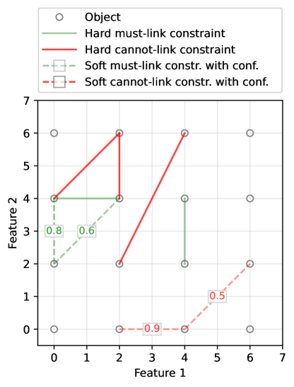
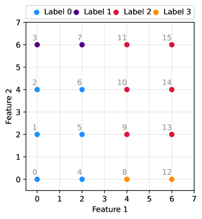
Figure 1: Illustrative example: input data (left) and ground truth (right). Here all pairwise relationships comply with the ground truth assignment.

3 Related literature

Many different algorithms have been proposed for clustering with must-link and cannot-link constraints. We focus our review on clustering algorithms that take the number of clusters $k$ as an input parameter and assign each object to exactly one cluster. Algorithms that determine the number of clusters $k$ internally or algorithms that assign objects in a soft manner, such as mixture model-based algorithms or fuzzy algorithms, are not considered here. We categorize the algorithms according to their methodology into exact, center-based, and non-center based algorithms. The three groups are discussed in Sections 3.1–3.3. Table 1 lists for each algorithm the methodology used, the clustering objective (e.g., k-means), and whether the objects are assigned sequentially to clusters or simultaneously. The checkmarks in the table indicate which elements of the constrained clustering problem described in the previous section are covered by the respective algorithms. A checkmark in the column “user-defined penalty” means the user can specify a penalty value for constraint violations. This option is useful when must-link and cannot-link constraints are noisy because it allows to control the balance between the clustering objective and the constraint violations, see Baumann and Hochbaum (2022). Algorithms that allow the user to define penalty values individually for the soft must-link and cannot-link constraint have an additional checkmark in the column “pairwise-specific penalties”. The approaches from the literature that we test in our experiments are highlighted in bold, both in the text and in Table 1.

Name	Method	Objective	Object	Hard	Hard	Soft	Soft	User-	Pairwise-
			assign-	ML	CL	ML	CL	defined	specific
			ment					penalty	penalties
CP	exact	multiple	simult.	$\checkmark$	$\checkmark$
CG	exact	wcss	simult.	$\checkmark$	$\checkmark$
BACT	exact	k-means	simult.	$\checkmark$	$\checkmark$
COPKM	center-based	k-means	sequent.	$\checkmark$	$\checkmark$
PCKM	center-based	k-means + pen.	sequent.			$\checkmark$	$\checkmark$	$\checkmark$
CVQE	center-based	k-means + pen.	sequent.			$\checkmark$	$\checkmark$
LCVQE	center-based	k-means + pen.	sequent.			$\checkmark$	$\checkmark$
LCC	center-based	k-means + pen.	sequent.	$\checkmark$	($\checkmark$)		($\checkmark$)
BCKM	center-based	k-means	simult.	$\checkmark$	$\checkmark$
BLPKM	center-based	k-means	simult.	$\checkmark$	$\checkmark$
BHKM	center-based	k-means + pen.	simult.			$\checkmark$	$\checkmark$	$\checkmark$
CSC	graph-based	cost of cut	simult.	($\checkmark$)	($\checkmark$)	$\checkmark$	$\checkmark$	$\checkmark$	$\checkmark$
DILS	metaheur.	wcss + pen.	simult.			$\checkmark$	$\checkmark$
SHADE	metaheur.	wcss + pen.	simult.			$\checkmark$	$\checkmark$
PCCC	center-based	k-means + pen.	simult.	$\checkmark$	$\checkmark$	$\checkmark$	$\checkmark$	$\checkmark$	$\checkmark$

Table 1: Overview of algorithms for clustering with must-link (ML) and cannot-link (CL) constraints. The checkmarks in the table indicate which elements of the constrained clustering problem described in the previous section are covered by the respective algorithms. A checkmark in parenthesis means that an element is only partly covered. The abbreviation wcss stands for within-cluster sum of squares. The algorithms highlighted in bold are included in our computational experiments.

3.1 Exact algorithms

Thanks to algorithmic advances and improvements in hardware (see e.g. Bertsimas and Dunn 2017), exact approaches are increasingly being used to optimally solve small instances of constrained clustering problems.

Dao et al. (2013) propose an exact approach for constrained clustering based on constraint programming (CP). The approach is flexible as it allows to integrate various types of constraints, including hard must-link and cannot-link constraints, and it allows to choose between different clustering objectives.

Another exact approach (CG) is proposed by Babaki et al. (2014). They introduce a column generation approach for the minimum within-cluster sum of squares (wcss) problem with additional constraints. The additional constraints include must-link and cannot-link constraints among other constraints.

Piccialli et al. (2022) propose an exact approach based on the branch-and-cut technique where must-link and cannot-link constraints are incorporated as hard constraints. The algorithm uses the binary-linear-programming-based k-means algorithm (BLPKM) of Baumann (2020) as a subroutine to obtain high-quality feasible solutions quickly. In Table 1, we use the abbreviation BACT (branch-and-cut technique) to refer to this approach.

The above-mentioned exact approaches do not consider soft constraints and are only applicable to small instances with up to around 1,000 objects. As we are interested in tackling much larger instances, we did not include exact approaches in our computational experiments.

3.2 Center-based algorithms

Most algorithms for clustering with must-link and cannot-link constraints are center-based. Center-based approaches identify a center for each cluster and aim to minimize the distances between the center of a cluster and the objects that belong to this cluster. The most well-known center-based algorithm for unconstrained clustering is the k-means algorithm.

Wagstaff et al. (2001) introduced a variant of the k-means algorithm, referred to as the COP-kmeans algorithm (COPKM), which incorporates the must-link and cannot-link constraints as hard constraints. It assigns objects sequentially to the closest feasible cluster center, i.e., an assignment is only possible if it does not violate a must-link or a cannot-link constraint. The algorithm stops without a solution if an object cannot be assigned to a cluster center without violating a must-link or a cannot-link constraint. The main drawback of the COP-kmeans algorithm is that the sequential assignment strategy often fails to find a feasible assignment, even if one exists.

The pairwise-constrained k-means algorithm of Basu et al. (2004) (PCKM) also assigns objects sequentially but allows constraint violations. An object is assigned to a cluster such that the sum of the object’s distance to the cluster center and the cost of constraint violations incurred by that assignment is minimized. The user can set a penalty for violating a constraint. The PCKM algorithm is not suited for settings where the must-link and cannot-link constraints are noisy because the procedure determining the starting positions of the cluster centers assumes that the must-link and cannot-link constraints are correct.

The constrained vector quantization algorithm (CVQE) of Davidson and Ravi (2005) is similar to the PCKM algorithm in that it assigns objects sequentially and allows for constraint violations. However, in the assignment step, pairs of objects subject to a constraint are simultaneously assigned to clusters such that an objective function which includes penalties for violated constraints, is increased as little as possible. To determine these clusters, the increase in the objective function must be calculated for each possible combination of clusters resulting in $O(k^{2})$ calculations for every constraint, where k denotes the number of clusters. The user cannot control the penalties for violating must-link and cannot-link constraints. Instead, the penalty for violating a must-link constraint corresponds to the distance between the centers of the two clusters that contain the two objects. Similarly, the penalty for violating a cannot-link constraint corresponds to the distance between the center of the cluster that contains both objects and the nearest center to one of the objects of another cluster.

The linear CVQE algorithm (LCVQE) of Pelleg and Baras (2007) is a modification of the CVQE algorithm with reduced computational complexity.

Ganji et al. (2016) introduce the Lagrangian Constrained Clustering (LCC) algorithm, a k-means style algorithm for constrained clustering that aims to satisfy as many pairwise constraints as possible. The algorithm first contracts objects that are connected by must-link constraints. This guarantees that all must-link constraints are satisfied and reduces the problem size. In the assignment step, objects are first assigned to their closest clusters. Then, for each violated cannot-link constraint, the algorithm decides to reassign one of the two involved objects to the second nearest cluster based on a penalty value associated with the constraint. In the update step, the positions of the cluster centers are moved such that an objective function that consists of distances and penalized constraint violations is minimized. A Lagrangian relaxation scheme ensures that penalties of cannot-link constraints that remain unsatisfied in subsequent iterations are increased. Because the penalties are dynamically adjusted during the algorithm’s execution, the user can’t specify an overall penalty for constraint violations or specific penalties for individual constraints. The algorithm terminates after a fixed number of iterations without improvement or after a maximum number of iterations. Because of this iteration limit and the fact that only reassignments of objects to the second nearest clusters are considered, the algorithm may terminate with an assignment that violates some of the cannot-link constraints even if there exists an assignment that satisfies all cannot-link constraints. Therefore, we put a checkmark in parentheses in the column “Hard CL” in Table 1.

Le et al. (2019) formulate the minimum within-cluster sum of squares problem with must-link and cannot-link constraints as a binary optimization problem, which they refer to as binary optimization-based constrained k-means (BCKM). An optimization strategy is proposed that iteratively updates the cluster center variables and the assignment variables. To update the assignment variables, the binary constraints are relaxed, and a linear program is solved. The solution is projected back to the binary domain using a technique related to the feasibility pump heuristic of Fischetti et al. (2005). Constraints on the cluster cardinalities can be incorporated as well. Computational results are reported for synthetic data sets with 500 objects and real-world data sets. The BCKM algorithm treats all pairwise constraints as hard constraints. The publicly available implementation of the BCKM algorithm can only deal with must-link constraints but not with cannot-link constraints. We, therefore, did not include this algorithm in our computational analysis.

The recently introduced binary linear programming-based k-means algorithm (BLPKM) algorithm of Baumann (2020) is a variant of the k-means algorithm that assigns objects to clusters by solving a binary linear optimization program in each iteration. The binary linear program includes the must-link and cannot-link constraints as hard constraints. Baumann and Hochbaum (2022) present a version of the BLPKM algorithm, referred to as BH-kmeans (BHKM), that includes the must-link and cannot-link constraints as soft constraints. Note that the PCCC algorithm that we introduce in this paper can be seen as a combination of the BLPKM and the BH-kmeans algorithms because it inherits the treatment of pairwise relationships as hard constraints from the BLPKM algorithm and the treatment of relationships as soft constraints from the BH-kmeans algorithm. In addition, the PCCC algorithm can account for constraint-specific confidence values and features two enhancements that improve scalability.

3.3 Non-center based algorithms

Wang et al. (2014) propose a spectral clustering-based algorithm (CSC) for clustering with must-link and cannot-link constraints. The pairwise constraints are encoded as an $n\times n$ constraint matrix that contains real numbers. A positive entry indicates that the corresponding objects belong to the same cluster, and a negative entry indicates that the corresponding objects belong to different clusters. A zero indicates that there is no information on the corresponding pair. The magnitude of the entries indicates how strong the belief is. Given a cluster assignment, a real-valued measure can be computed that quantifies the overall constraint satisfaction. The CSC algorithm solves a constrained spectral clustering problem through generalized eigendecomposition such that a user-defined lower bound on the constraint satisfaction is guaranteed. We put the checkmarks in the columns “Hard ML” and “Hard CL” in Table 1 in parentheses because the algorithm is not applicable to instances where it must be guaranteed that individual constraints are satisfied. Zhi et al. (2013) propose a framework for spectral clustering that allows to incorporate logical combinations of constraints that are more complex than must-link and cannot-link constraints. They propose a quadratic programming formulation that contains the logical constraints as linear equalities and inequalities.

González-Almagro et al. (2020) introduced the dual iterative local search algorithm (DILS). The DILS algorithm is an evolution-based metaheuristic that employs mutation and recombination operations and a local search procedure to improve solutions, similar to a genetic algorithm. However, the DILS algorithm only keeps two solutions in memory at all times. González-Almagro et al. (2020) demonstrated the superiority of the DILS algorithm over established algorithms in terms of solution quality in a computational experiment. The main drawback of the DILS algorithm is the substantial running time requirement which hinders its use for large data sets. The DILS algorithm treats all must-link and cannot-link constraints as soft constraints and thus cannot guarantee that any hard constraints are satisfied. Another drawback is that the user cannot specify a penalty for violating a must-link or soft-link constraint. Instead, the fitness function multiplies the within-cluster-sum-of-squares with the number of unsatisfied constraints.

González-Almagro et al. (2021) propose a differential evolution-based algorithm (SHADE) for clustering with must-link and cannot-link constraints. Their algorithm achieves similar, although on average slightly worse, ARI values than the DILS algorithm on the benchmark instances used in González-Almagro et al. (2020). We therefore do not test it in our computational experiments.

4 Our PCCC algorithm

The PCCC algorithm consists of five steps: preprocessing, initialization, assignment, update, and postprocessing. Figure 2 provides a flowchart of the algorithm. Like in the well-known k-means algorithm, the assignment and the update step are repeated until a stopping criterion is reached. In Sections 4.1–4.5, we describe all five steps in detail. Figure 3 illustrates the steps of the flowchart with the illustrative example from Section 2.3.

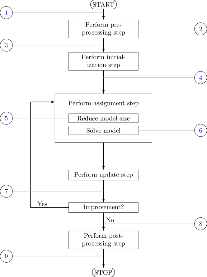
Figure 2: Flowchart of the PCCC algorithm. Illustrations 1–9 are given in Figure 3

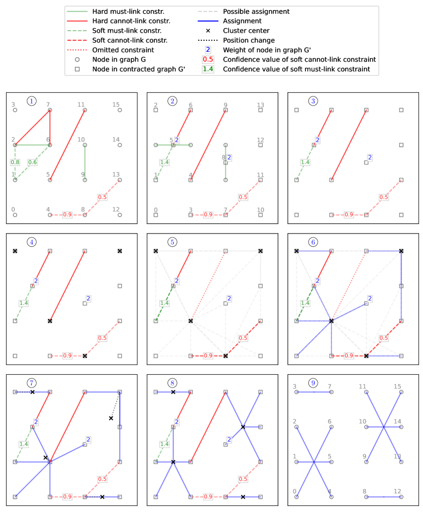
Figure 3: Illustrations for flowchart based on the illustrative example. The input consists of $n=16$ objects that are described by 2 features. The goal is to partition this data set into $k=4$ clusters. The additional information consists of three hard cannot-link constraints, two hard must-link constraints, two soft cannot-link constraints, and two soft must-link constraints. The algorithm is applied with parameter $q=2$, which explains why the hard cannot-link constraint between the contracted nodes 4 and 9 can be omitted in the assignment step (see illustrations 5 and 6).

The input data consists of a set of $n$ objects, each is represented by a $d$-dimensional numeric feature vector $\boldsymbol{x}_{i}\in\mathbb{R}^{d}$, a parameter $k$ that determines the number of clusters to be identified, and the additional information consisting of the sets or pairwise constraints $ML$, $CL$, $SML$, $SCL$, and the associated confidence values (see Section 2.1). The input data is represented as a weighted undirected graph $G=(V,E)$ where the node set $V$ corresponds to the objects, and the edge set $E$ corresponds to the pairwise constraints. We distinguish four types of edges: the edges $E^{\textup{ML}}$ correspond to the hard must-link constraints from set $ML$, the edges $E^{\textup{CL}}$ correspond to the hard cannot-link constraints from set $CL$, the edges $E^{\textup{SML}}$ correspond to the soft must-link constraints from set $SML$, and the edges $E^{\textup{SCL}}$ correspond to the soft cannot-link constraints from set $SCL$. The edges representing soft constraints are associated with a confidence value $w_{ij}$. Table 2 provides the graph notation that we use in the subsequent sections.

Input data
$G=(V,E)$	Weighted undirected graph that represents the input data
$V$	Nodes representing objects
$E$	Edges representing additional information
$E^{\textup{ML}}\subseteq E$	Edges representing hard must-link constraints
$E^{\textup{CL}}\subseteq E$	Edges representing hard cannot-link constraints
$E^{\textup{SML}}\subseteq E$	Edges representing soft must-link constraints
$E^{\textup{SCL}}\subseteq E$	Edges representing soft cannot-link constraints
$w_{ij}$	Weight of edge $\{i,j\}\in E^{\textup{SML}}\cup E^{\textup{SCL}}$
$k$	Number of clusters to be identified
$\boldsymbol{x}_{i}\in\mathbb{R}^{d}$	Feature vector of node $i$
Input data after preprocessing
$G^{\prime}=(V^{\prime},E^{\prime})$	Weighted undirected graph after node contraction
$V^{\prime}$	Nodes in contracted graph
$E^{\prime}$	Edges in contracted graph
$E^{\prime\textup{CL}}\subseteq E^{\prime}$	Edges representing hard cannot-link constraints in contracted graph
$E^{\prime\textup{SML}}\subseteq E^{\prime}$	Edges representing soft must-link constraints in contracted graph
$E^{\prime\textup{SCL}}\subseteq E^{\prime}$	Edges representing soft cannot-link constraints in contracted graph
$m(i)$	Mapping of a node $i\in V$ to a node in $V^{\prime}$
$w^{\prime}_{ij}$	Weight of edge $(i,j)\in E^{\prime\textup{SML}}\cup E^{\prime\textup{SCL}}$
$s_{i}$	Weight of node $i$
$\boldsymbol{\bar{x}}_{i}\in\mathbb{R}^{d}$	Feature vector of node $i\in V^{\prime}$

Table 2: Description of graph notation

4.1 Preprocessing step

In the preprocessing step, we transform graph $G$ into a new graph $G^{\prime}=(V^{\prime},E^{\prime})$ by contracting all edges $\{i,j\}\in E^{\textup{ML}}$ which represent hard must-link constraints. These edge contractions merge each group of nodes that is directly or indirectly connected by hard must-link edges into a single node. Let set $V_{i}$ denote the nodes of graph $G$ that are merged into node $i$ of the new graph $G^{\prime}$. The mapping $m:V\rightarrow V^{\prime}$ indicates for each node in graph $G$ the corresponding node in the new graph. Each node $i\in V^{\prime}$ is associated with a weight $s_{i}$ that indicates how many nodes of graph $G$ were merged into this node. The feature vector $\boldsymbol{\bar{x}}_{i}$ of node $i\in V^{\prime}$ is computed as $\boldsymbol{\bar{x}}_{i}=\frac{\sum_{j\in V_{i}}\boldsymbol{x}_{j}}{s_{i}}$. The edge set $E^{\prime}$ of the new graph $G^{\prime}$ consists of edges representing hard cannot-link constraints $E^{\prime\textup{CL}}=\{\{m(i),m(j)\}|\{i,j\}\in E^{\textup{CL}}\}$, edges representing soft must-link constraints $E^{\prime\textup{SML}}=\{\{m(i),m(j)\}|\{i,j\}\in E^{\textup{SML}}\wedge m(i)\neq m(j)\}$, and edges representing soft cannot-link constraints $E^{\prime\textup{SCL}}=\{\{m(i),m(j)\}|\{i,j\}\in E^{\textup{SCL}}\wedge m(i)\neq m(j)\}$. In case $E^{\prime CL}$ contains edges $\{i,j\}$ with $i=j$, then we know that there is no feasible assignment. The weights $w^{\prime}_{ij}$ of the edges $\{i,j\}\in E^{\prime\textup{SML}}$ are computed as $w^{\prime}_{ij}=\sum_{\{i^{\prime},j^{\prime}\}\in E^{\textup{SML}}|m(i^{\prime})=i\wedge m(j^{\prime})=j}w_{i^{\prime}j^{\prime}}$. The weights $w^{\prime}_{ij}$ of the edges $\{i,j\}\in E^{\prime\textup{SCL}}$ are computed as $w^{\prime}_{ij}=\sum_{\{i^{\prime},j^{\prime}\}\in E^{\textup{SCL}}|m(i^{\prime})=i\wedge m(j^{\prime})=j}w_{i^{\prime}j^{\prime}}$. If a pair of nodes $\{i,j\}$ is contained in both edge sets $E^{\prime SML}$ and $E^{\prime SCL}$, then we remove the edge with the smaller weight and adjust the other weight by subtracting the smaller weight from it. The output of the preprocessing step is the transformed input data represented as graph $G^{\prime}$.

4.2 Initialization step

In the initialization step, we determine the initial positions of the $k$ cluster centers. We provide two different methods for this step. The first method randomly selects $k$ distinct nodes in graph $G^{\prime}$ and uses their feature vectors $\boldsymbol{\bar{x}}_{i}$ as initial positions. This method is fast but might select some initial positions close to each other so that convergence will be slow. The second method is the k-means++ algorithm of Arthur and Vassilvitskii (2007). The k-means++ algorithm requires extra running time but tends to spread out the initial positions, which speeds up convergence.

4.3 Assignment step

In the assignment step, each node in graph $G^{\prime}$ is assigned to one of the $k$ clusters such that the total distance between the nodes and the centers of their assigned clusters is minimized subject to the hard and soft pairwise constraints. We solve the mixed binary linear program (MBLP) presented below to assign the nodes to clusters. Table 3 describes the notation used in the formulation.

Table 3: Additional notation used in formulation (MBLP)

Additional parameters
$d_{il}$	Euclidean distance between node $i\in V^{\prime}$ and the center of cluster $l$
$P$	Penalty value (by default: $P=\sum_{i\in V^{\prime};~{}l=1\ldots,k}d_{il}/|V^{\prime}|$)
Binary decision variables
$x_{il}$	=1, if node $i\in V^{\prime}$ is assigned to cluster $l$; =0, otherwise
Continuous decision variables
$y_{ij}$	Auxiliary variables to capture violations of soft cannot-link constraint
$z_{ij}$	Auxiliary variables to capture violations of soft must-link constraints

$$\textup{(MBLP)}\left\{\begin{array}[]{lllr}\textup{Min.}&\lx@intercol\displaystyle\sum_{i\in V^{\prime}}\sum_{l=1}^{k}s_{i}d_{il}x_{il}+P\left(\sum_{\{i,j\}\in E^{\prime\textup{SCL}}}w^{\prime}_{ij}y_{ij}+\sum_{\{i,j\}\in E^{\prime\textup{SML}}}w^{\prime}_{ij}z_{ij}\right)\hfil\lx@intercol&(1)\\ \textup{s.t.}&\displaystyle\sum_{l=1}^{k}x_{il}=1&(i\in V^{\prime})&(2)\\ &\displaystyle\sum_{i\in V^{\prime}}x_{il}\geq 1&(l=1,\ldots,k)&(3)\\ \vspace{-0.2cm}&\displaystyle x_{il}+x_{jl}\leq 1&(\{i,j\}\in E^{\prime\textup{CL}};~{}l=1,\ldots,k)&(4)\\ \vspace{-0.2cm}&\displaystyle x_{il}+x_{jl}\leq 1+y_{ij}&(\{i,j\}\in E^{\prime\textup{SCL}};~{}l=1,\ldots,k)&(5)\\ \vspace{-0.2cm}&\displaystyle x_{il}-x_{jl}\leq z_{ij}&(\{i,j\}\in E^{\prime\textup{SML}};~{}l=1,\ldots,k)&(6)\\ \vspace{-0.2cm}&x_{il}\in\{0,1\}&(i\in V^{\prime};~{}l=1,\ldots,k)&(7)\\ \vspace{-0.2cm}&y_{ij}\geq 0&\{i,j\}\in E^{\prime\textup{SCL}}&(8)\\ \vspace{-0.2cm}&z_{ij}\geq 0&\{i,j\}\in E^{\prime\textup{SML}}&(9)\end{array}\right.$$

The objective function includes two terms. The first term computes the total weighted Euclidean distance between the feature vectors of the nodes $i\in V^{\prime}$ and the centers of their assigned clusters. The second term computes the total penalty value that results from violating soft cannot-link and soft must-link constraints. Each violation is weighted by $w^{\prime}_{ij}$ and multiplied with parameter $P$, which trades off the weighted violations against the weighted distances from the first term in the objective function. Parameter $P$ is a control parameter that the user can choose. If the user chooses $P$, it does not change during the algorithm’s execution. If the user does not specify a value, we set parameter $P$ as the average distance between a node and a cluster center. The average distance is recomputed in each iteration to account for changing distances between the nodes and the cluster centers. Constraints (2) ensure that each node is assigned to exactly one cluster. Constraints (3) prevent empty clusters by requiring that at least one node is assigned to each cluster. Constraints (4) represent the hard cannot-link constraints. Constraints (5) represent the soft cannot-link constraints. If a pair of nodes $\{i,j\}\in E^{\prime\textup{SCL}}$ is assigned to the same cluster $l$, then the auxiliary variable $y_{ij}$ is forced to take value one which adds the penalty $Pw^{\prime}_{ij}$ to the objective function. Constraints (6) represent the soft must-link constraints. If a pair of nodes $\{i,j\}\in E^{\prime\textup{SML}}$ is assigned to different clusters, then for one $l=1,\ldots,k$, the left-hand side of constraint (6) will be one, and thus forces the auxiliary variable $z_{ij}$ to take value one which adds the penalty $Pw^{\prime}_{ij}$ to the objective function. Constraints (7)–(9) define the domains of the decision variables.

In order to reduce the size of the formulation when the number of clusters, $k$, is large, we allow to assign a node only to one of the $q$ nearest clusters, where the distance of the node from a cluster is determined by the distance to its center. Without any pairwise constraints, every node is assigned to the nearest cluster in an optimal assignment. With pairwise constraints, the nodes might not be assigned to their nearest center in order to satisfy the constraints. However, rarely will nodes be assigned to distant centers even in the presence of pairwise constraints. For simplicity, we hereafter refer to the distance between a node and a cluster center as the distance between a node and a cluster. By allowing only assignments between a node $i$ and its $q$ nearest clusters, we can reduce the number of binary decision variables from $|V^{\prime}|k$ to $|V^{\prime}|q$. The $q$ nearest clusters can be efficiently determined using kd-trees when the number of features is much smaller than the number of nodes (see Bentley 1975). We refer to the reduced mixed binary linear program as (R($q$)MBLP) as it depends on the choice of control parameter $q$. If there are no hard cannot-link constraints, the user can choose parameter $q$ arbitrarily to control the trade-off between model size and flexibility to satisfy pairwise constraints. Lower values for $q$ result in smaller formulations but fewer possibilities to satisfy the pairwise constraints. If there are hard cannot-link constraints, we need to set parameter $q$ sufficiently large to guarantee that we can find a feasible assignment if one exists. Let $H=(V^{\prime},E^{\prime\textup{CL}})$ be a subgraph of graph $G^{\prime}$ that has the same node set $V^{\prime}$ as graph $G^{\prime}$, but whose edge set only contains the edges that correspond to hard cannot-link constraints. The expression $\textup{deg}_{H}(i)$ denotes the degree of node $i$ in subgraph $H$ and $\Delta(H)$ is the maximum degree of the nodes in $H$, i.e., $\Delta(H)=\max_{i\in V^{\prime}}\textup{deg}_{H}(i)$.

Lemma 1

If a feasible assignment exists, we find a feasible assignment by solving model (R($q$)MBLP) with $q\geq\min(1+\Delta(H),k)$.

Proof  The problem of finding an assignment that satisfies all hard cannot-link constraints corresponds to solving a $k$-coloring problem on graph $H=(V^{\prime},E^{\prime\textup{CL}})$. The $k$-coloring problem on graph $H$ consists of assigning one of $k$ colors to each node $i\in V^{\prime}$ such that all adjacent nodes have different colors. A feasible solution using at most $k$ colors is called a $k$-coloring. The chromatic number of graph $H$, denoted as $\chi(H)$, is the smallest number of colors required to color the nodes of graph $H$ such that no two adjacent nodes have the same color. Hence, we are guaranteed to find a feasible assignment (assuming one exists) as long as $q\geq\chi(H)$. From Welsh and Powell (1967), we know that graph $H$ can be colored with at most $\Delta(H)+1$ colors. Hence $\Delta(H)+1$ is an upper bound on $\chi(H)$. Consequently, if a feasible assignment exists, we are guaranteed to find it with $q\geq\Delta(H)+1$.  

Table 4: Additional notation used in formulation (R($q$)MBLP)

$G^{\prime\prime}=(V^{\prime},E^{\prime\prime})$	Subgraph of graph G’
$E^{\prime\prime}$	Edges in subgraph $G^{\prime\prime}$
$E^{\prime\prime\textup{CL}}$	Edges representing hard cannot-link constraints
$E^{\prime\prime\textup{SCL}}$	Edges representing soft cannot-link constraints
$E^{\prime\prime\textup{SML}}$	Edges representing soft must-link constraints
Sets
$L_{i}$	Clusters to which node $i$ can be assigned
$V^{\prime}_{l}$	Nodes that can be assigned to cluster $l$

Next, we present the reduced mixed binary linear program (R($q$)MBLP) that we solve if we apply the model size reduction technique described above. Let $L_{i}$ denote the set of $q$ nearest clusters to node $i$. If a cluster does not belong to the $q$ nearest clusters of any node, we add it to set $L_{i}$ of its closest node $i$. This guarantees that at least one node can be assigned to each cluster. Some hard and soft cannot-link constraints become redundant if we require nodes to be assigned to one of their $q$ nearest clusters. For example, if two nodes $\{i,j\}\in E^{\prime\textup{CL}}$ cannot be assigned to the same cluster because $L_{i}\cap L_{j}=\emptyset$, the respective cannot-link constraint does not need to be included in the reduced mixed binary linear program. We introduce the following two new sets of edges that represent hard and soft cannot-link constraints: $E^{\prime\prime\textup{CL}}=\{\{i,j\}\in E^{\prime\textup{CL}}|L_{i}\cap L_{j}\neq\emptyset\}$, $E^{\prime\prime\textup{SCL}}=\{\{i,j\}\in E^{\textup{SCL}}|L_{i}\cap L_{j}\neq\emptyset\}$. These sets represent only hard and soft cannot-link constraints that can still be violated after applying the reduction technique. Some soft must-link constraints may automatically be violated if we require nodes to be assigned to one of their $q$ nearest clusters. We introduce the following set of soft must-link pairs: $E^{\prime\prime\textup{SML}}=\{\{i,j\}\in E^{\prime\textup{SML}}|L_{j}\cap L_{j^{\prime}}\neq\emptyset\}$. This set only contains the soft must-link constraints that can potentially be satisfied after applying the reduction technique. Table 4 describes the additional notation used in the reduced mixed binary linear program (R($q$)MBLP), which reads as follows.

$$\textup{(R($q$)MBLP)}\left\{\begin{array}[]{lllr}\textup{Min.}&\lx@intercol\displaystyle\sum_{i\in V^{\prime}}\sum_{l\in L_{i}}s_{i}d_{il}x_{il}+P\left(\sum_{\{i,j\}\in E^{\prime\prime\textup{SCL}}}w^{\prime}_{ij}y_{ij}+\sum_{\{i,j\}\in E^{\prime\prime\textup{SML}}}w^{\prime}_{ij}z_{ij}\right)\hfil\lx@intercol&(1)\\ \textup{s.t.}&\displaystyle\sum_{l\in L_{i}}x_{il}=1&(i\in V^{\prime})&(2)\\ &\displaystyle\sum_{i\in V^{\prime}_{l}}x_{il}\geq 1&(l=1,\ldots,k)&(3)\\ &x_{il}+x_{jl}\leq 1&(\{i,j\}\in E^{\prime\prime\textup{CL}};~{}l\in L_{i}\cap L_{j})&(4)\\ &x_{il}+x_{jl}\leq 1+y_{ij}&(\{i,j\}\in E^{\prime\prime\textup{SCL}};~{}l\in L_{i}\cap L_{j})&(5)\\ &x_{il}-x_{jl}\leq z_{ij}&(\{i,j\}\in E^{\prime\prime\textup{SML}};~{}l\in L_{i}\cap L_{j})&(6)\\ &x_{il}\leq z_{ij}&(\{i,j\}\in E^{\prime\prime\textup{SML}};~{}l\in L_{i}\setminus L_{j})&(7)\\ &x_{jl}\leq z_{ij}&(\{i,j\}\in E^{\prime\prime\textup{SML}};~{}l\in L_{j}\setminus L_{i})&(8)\\ \vspace{-0.2cm}&x_{il}\in\{0,1\}&(i\in V^{\prime};~{}l\in L_{i})&(9)\\ \vspace{-0.2cm}&y_{ij}\geq 0&\{i,j\}\in E^{\prime\prime\textup{SCL}}&(10)\\ \vspace{-0.2cm}&z_{ij}\geq 0&\{i,j\}\in E^{\prime\prime\textup{SML}}&(11)\end{array}\right.$$

Most of the constraints of the model (R($q$)MBLP) are similar to the constraints of the model (MBLP) and are thus not further explained here. Constraints (7) are required to ensure that $z_{ij}$ takes value one if node $i$ is assigned to a cluster $l$ that is not among the $q$ nearest centers of node $j$. Analogously, constraints (8) ensure that $z_{ij}$ takes value one if node $j$ is assigned to a cluster $l$ that is not among the $q$ nearest centers of node $i$.

4.4 Update step

In the update step, the positions of the cluster centers are adjusted based on the assignment of nodes to clusters determined in the previous assignment step. We denote the positions of the cluster centers as $\boldsymbol{\bar{o}}_{l}$. The computation of the new positions takes into account the weights $s_{i}$ of the nodes. Let $A_{l}$ be the set of nodes assigned to cluster $l$. The position of the center of cluster $l$ is then computed as $\boldsymbol{\bar{o}}_{l}=\frac{\sum_{i\in A_{l}}s_{i}\boldsymbol{\bar{x}}_{i}}{\sum_{i\in A_{l}}s_{i}}$. The assignment and the update steps are repeated as long as the objective function of the (reduced) mixed binary linear program (R($q$)MBLP), computed after the update step, can be decreased. The best assignment at termination is passed to the postprocessing step.

4.5 Postprocessing step

In the postprocessing step, we map the labels of the nodes $i\in V^{\prime}$ back to the original objects and return the final assignment to the user.

5 Computational experiments

In this section, we compare the PCCC algorithm to state-of-the-art approaches. Since the state-of-the-art approaches are less general in their applicability than the PCCC algorithm, we focus on instances to which all approaches are applicable. In Section 5.1, we list the state-of-the-art approaches. In Section 5.2, we introduce the three collections of data sets that we use in the computational experiments. In Section 5.3, we describe the constraint sets that accompany the data sets. In Sections 5.4–5.6, we report and discuss the results of the algorithms for the three different data set collections, respectively. All experiments were executed on an HP workstation with two Intel Xeon CPUs with clock speed 3.30 GHz and 256 GB of RAM.

5.1 State-of-the-art approaches

The DILS algorithm of González-Almagro et al. (2020) represents the current state-of-the-art in terms of the Adjusted Rand Index (ARI). In a recent computational comparison, it outperformed six established algorithms for clustering with must-link and cannot-link constraints (see González-Almagro et al. 2020). We, therefore, include the DILS algorithm in our experiments. In addition, we include the Lagrangian Constrained Clustering (LCC) algorithm of Ganji et al. (2016) and the spectral clustering-based algorithm (CSC) of Wang et al. (2014) as they have not yet been compared to the DILS algorithm in the literature. Although the COP-Kmeans algorithm (COPKM) of Wagstaff et al. (2001) is one of the algorithms that was outperformed by the DILS algorithm, we include it in our experiments because it is probably the most popular algorithm for clustering with must-link and cannot-link constraints and thus provides a valuable point of reference. Finally, to assess the impact of considering pairwise constraints, we also include the unconstrained k-means algorithm, which disregards all pairwise constraints. Table 5 lists for each tested approach the corresponding paper and the programming language of the implementation.

Name	Paper	Code
Kmeans (KMEANS)	MacQueen et al. (1967)	Python
COP-Kmeans (COPKM)	Wagstaff et al. (2001)	Python
Constrained spectral clustering (CSC)	Wang et al. (2014)	Matlab
Lagrangian constrained clustering (LCC)	Ganji et al. (2016)	R
Dual iterative local search (DILS)	González-Almagro et al. (2020)	Python
PCCC algorithm (PCCC)	This paper	Python

Table 5: Overview of tested approaches

5.2 Data sets

We use three collections of data sets, which we refer to as COL1, COL2, and COL3. All data sets are classification data sets, i.e., a ground truth assignment is available to evaluate the clustering solution with an external performance measure such as the Adjusted Rand Index (ARI). Table 6 provides an overview of the three collections.

Table 6: The table reports for each collection the number of data sets, the minimum and maximum size of a data set in the collection in terms of number of objects, number of features, and number of classes (here clusters), and the type

Collection name	Data sets	Objects	Features	Classes	Type
COL1	25	47–846	2–90	2–15	Real and syntehtic
COL2	24	500–5,000	2–2	2–100	Syntehtic
COL3	6	5,300–70,000	2–3,072	2–100	Real and syntehtic

Collection COL1 contains the 25 data sets used in González-Almagro et al. (2020). The data sets of this collection are of sizes up to 846 objects, 90 features, and 15 classes. We use this collection to compare the proposed approach to state-of-the-art algorithms on well-known benchmark data sets from the literature. Collection COL1 contains data sets with irregular shapes that the standard (unconstrained) k-means algorithm fails to detect. We downloaded the data sets using the links provided in González-Almagro et al. (2020). In the data set Saheart, we replaced the two non-numeric categories Present and Absent of the feature “Famhist” with one and zero, respectively. We standardized the features of each data set by removing the mean and scaling to unit variance. Table 7 lists the main characteristics of these data sets.

Table 7: Characteristics of data sets from collection COL1

Data set	Objects	Features	Classes	Type	Source
Appendicitis	106	7	2	real	Keel
Breast Cancer	569	30	2	real	Sklearn
Bupa	345	6	2	real	Keel
Circles	300	2	2	synthetic	GitHub
Ecoli	336	7	8	real	Keel
Glass	214	9	6	real	Keel
Haberman	306	3	2	real	Keel
Hayesroth	160	4	3	real	Keel
Heart	270	13	2	real	Keel
Ionosphere	351	33	2	real	Keel
Iris	150	4	3	real	Keel
Led7Digit	500	7	10	real	Keel
Monk2	432	6	2	real	Keel
Moons	300	2	2	synthetic	GitHub
Movement Libras	360	90	15	real	Keel
Newthyroid	215	5	3	real	Keel
Saheart	462	9	2	real	Keel
Sonar	208	60	2	real	Keel
Spectfheart	267	44	2	real	Keel
Spiral	300	2	2	synthetic	GitHub
Soybean	47	35	4	real	Keel
Tae	151	5	3	real	Keel
Vehicle	846	18	4	real	Keel
Wine	178	13	3	real	Keel
Zoo	101	16	7	real	Keel

Collection COL2 contains synthetic data sets of sizes up to 5,000 objects, 2 features, and 100 classes that we generated to systematically investigate the impact of complexity parameters such as the number of objects and the number of clusters on the performance of the clustering algorithms. We used the datasets.make_blobs() function from the scikit-learn package to generate the data sets (see Pedregosa et al. 2011). This function generates normally-distributed clusters of points. The number of objects, the number of features, the number of clusters, as well as the standard deviation of the clusters can be controlled by the user. We varied the number of objects and the number of clusters and used the default values for all other parameters of the datasets.make_blobs() function. The number of objects was chosen from the set {500, 1,000, 2,000, 5,000} and the number of clusters was chosen from the set {2, 5, 10, 20, 50, 100}. We generated one data set for each combination of these two complexity parameters. We standardized the features of each data set by removing the mean and scaling to unit variance. Table 8 lists the main characteristics of these data sets.

Table 8: Characteristics of data sets from collection COL2

Data set	Objects	Features	Classes	Type	Source
n500-k2	500	2	2	synthetic	Sklearn
n500-k5	500	2	5	synthetic	Sklearn
n500–k10	500	2	10	synthetic	Sklearn
n500-k20	500	2	20	synthetic	Sklearn
n500-k50	500	2	50	synthetic	Sklearn
n500-k100	500	2	100	synthetic	Sklearn
n1000-k2	1,000	2	2	synthetic	Sklearn
n1000-k5	1,000	2	5	synthetic	Sklearn
n1000-k10	1,000	2	10	synthetic	Sklearn
n1000-k20	1,000	2	20	synthetic	Sklearn
n1000-k50	1,000	2	50	synthetic	Sklearn
n1000-k100	1,000	2	100	synthetic	Sklearn
n2000-k2	2,000	2	2	synthetic	Sklearn
n2000-k5	2,000	2	5	synthetic	Sklearn
n2000-k10	2,000	2	10	synthetic	Sklearn
n2000-k20	2,000	2	20	synthetic	Sklearn
n2000-k50	2,000	2	50	synthetic	Sklearn
n2000-k100	2,000	2	100	synthetic	Sklearn
n5000-k2	5,000	2	2	synthetic	Sklearn
n5000-k5	5,000	2	5	synthetic	Sklearn
n5000-k10	5,000	2	10	synthetic	Sklearn
n5000-k20	5,000	2	20	synthetic	Sklearn
n5000-k50	5,000	2	50	synthetic	Sklearn
n5000-k100	5,000	2	100	synthetic	Sklearn

Collection COL3 contains large-sized data sets of sizes up to 70,000 objects, 3,072 features, and 100 clusters that we selected from three different sources (Keel repository, Cifar website, and Mnist database). This collection of data sets will be used to compare the scalability of the proposed approach with the state-of-the-art approaches. We standardized the features of each data set by removing the mean and scaling to unit variance. Table 9 lists the main characteristics of these data sets.

Table 9: Characteristics of data sets from collection COL3

Data set	Objects	Features	Classes	Type	Source
Banana	5,300	2	2	synthetic	Keel
Letter	20,000	16	26	real	Keel
Shuttle	57,999	9	7	real	Keel
Cifar 10	60,000	3,072	10	real	Cifar website
Cifar 100	60,000	3,072	100	real	Cifar website
Mnist	70,000	784	10	real	Mnist database

5.3 Constraint sets

An instance of the clustering problem described in Section 2.1 consists of a data set, a number of clusters to be identified, and additional information in the form of pairwise constraints. In this subsection, we describe how we generated the pairwise constraints for the data sets of the different collections. We followed the procedure of González-Almagro et al. (2020) to generate noise-free constraint sets. Noise-free constraints agree with the ground truth assignment of a data set, i.e., if two objects are subject to a must-link constraint, then they have the same ground truth label. If two objects are subject to a cannot-link constraint, they have two different ground truth labels. The procedure of González-Almagro et al. (2020) takes as input the ground truth labels $y_{1},\ldots,y_{n}$ of a data set with $n$ objects, and a user-defined percentage $p_{c}$ that determines the size of the constraint set. The size (the number of pairwise constraints) of a constraint set is computed as $\frac{\lceil p_{c}n\rceil(\lceil p_{c}n\rceil-1)}{2}$. Each constraint is then generated by randomly selecting two objects and comparing their ground truth labels. A must-link constraint is generated when the two labels are the same, and a cannot-link constraint is generated when the two labels are different. This procedure guarantees that all constraints are correct and that there is always a cluster assignment that satisfies all constraints.

González-Almagro et al. (2020) used their procedure to generate four constraint sets with $p_{c}\in\{0.05,0.1,0.15,0.2\}$ for each data set of collection COL1. Since these constraint sets are publicly available on google drive, we use the same constraint sets that González-Almagro et al. (2020) generated with their procedure. This is except for the two data sets, Iris and Wine. We found that the constraint sets of these two data sets contained must-link and cannot-link constraints that do not agree with the ground truth. We therefore generated four new constraint sets for each of these two data sets with the above-described procedure of González-Almagro et al. (2020) and $p_{c}\in\{0.05,0.1,0.15,0.2\}$. Based on the percentage $p_{c}$, we refer to these four constraint set sizes as 5% CS, 10% CS, 15% CS, and 20% CS.

The data sets of collection COL2 are newly introduced in this paper. For each of these data sets, we generated five constraint sets with the procedure of González-Almagro et al. (2020) with $p_{c}\in\{0,0.05,0.1,0.15,0.2\}$. We refer to these four constraint set sizes as 0% CS, 5% CS, 10% CS, 15% CS, and 20% CS. The constraint sets of size 0% CS are empty constraint sets that we use to assess the performance of the algorithms when no additional information is provided.

No constraint sets have been presented in the literature for the data sets of collection COL3. We therefore used the procedure of González-Almagro et al. (2020) to generate three constraints sets for each of these data sets, one with $p_{c}=0.005$, one with $p_{c}=0.01$, and one with $p_{c}=0.05$. Due to the large number of objects in these datasets, these percentages already lead to a large number of constraints. For example, the constraint set associated with $p_{c}=0.05$ that we generate for the Mnist data set with $n=70,000$ contains 6,123,250 constraints. Based on the percentage $p_{c}$, we refer to these three constraint set sizes as 0.5% CS, 1% CS, 5% CS.

In addition to the above-mentioned noise-free constraint sets, we also generated noisy constraint sets for the data sets Appendicitis, Moons, and Zoo of collection COL1. These noisy constraint sets may contain incorrect constraints, i.e., constraints that do not agree with the ground truth labels. Each constraint in these noisy constraint sets is associated with a confidence value that indicates the reliability of the constraint. The noisy constraint sets allow us to investigate whether it is beneficial to account for confidence values if they are available. The generation procedure for the noisy constraint sets takes as input the ground truth labels $y_{1},\ldots,y_{n}$ of a data set with $n$ objects, a percentage $p_{c}$ that determines the number of constraints to be generated, and a lower bound $l\geq 0.5$ that determines the amount of noise in the constraint set. The number of constraints to be generated is computed as $\frac{\lceil p_{c}n\rceil(\lceil p_{c}n\rceil-1)}{2}$. For each constraint, we first randomly select a pair of objects $(i,j)$, then draw a probability value $o_{ij}$ from a uniform distribution over $[l,1)$, and finally draw a random value $r_{ij}$ from a uniform distribution over [0, 1). If the random value $r_{ij}$ is smaller or equal to the probability value $o_{ij}$, a correct constraint is generated, i.e. a must-link constraint if $y_{i}=y_{i^{\prime}}$ or a cannot-link constraint if $y_{i}\neq y_{i^{\prime}}$. A wrong constraint is generated if the random value is larger than the probability value. Hence, the probability value $o_{ij}$ corresponds to the probability that the constraint is correct. For the computational experiments with noisy constraints, we generated constraint sets with $p_{c}\in 0.05,0.1,0.15,0.2$ and $l=0.5,0.6,\ldots,1$. Note that when $l=1$, we set the probability values $o_{ij}=1$ for all pairs of objects. The confidence values $w_{ij}$ were computed based on the probability values $o_{ij}$ as follows: $w_{ij}=2(o_{ij}-0.5)$. This computation ensures that $w_{ij}=0$ if $o_{ij}=0.5$ and that $w_{ij}=1$ if $o_{ij}=1$. Table 10 illustrates the generation procedure for a data set with $n=100$ objects, a percentage $p_{c}=0.1$, and a lower bound $l=0.6$. Based on the percentage $p_{c}$, we refer to these three constraint set sizes as 5% NCS, 10% NCS, 15% NCS, an 20% NCS.

Constr.	Pair ($i,j$)	$y_{i}$	$y_{j}$	Probability value $o_{ij}$	Random number $r_{ij}$	Type
1	(13, 24)	1	1	0.73	0.91	cannot-link
2	(38, 43)	1	0	0.65	0.41	cannot-link
$\vdots$
44	(49, 56)	0	0	0.82	0.11	must-link
45	(71, 94)	0	1	0.92	0.83	cannot-link

Table 10: This table illustrates the process to generate noisy constraints for a data set with $n=100$ objects, a percentage $p_{c}=0.1$, and a lower bound $l=0.6$

Tables 11–13 in the appendix list the number of must-link and cannot-link constraints in the constraint sets of the collections COL1–COL3, respectively. The tables show that the ratio between the number of must-link and the number of cannot-link constraints varies greatly between constraint sets. The constraint sets associated with data sets with many classes tend to have more cannot-link constraints. The ratio between the number of must-link and cannot-link constraints strongly affects the difficulty of an instance. Instances with constraint sets that mostly contain cannot-link constraints are considered more challenging than instances with constraint sets that mostly contain must-link constraints.

We provide a code on GitHub for making the collections COL1, COL2, and COL3 and the constraint sets available. Running this code downloads the publicly available data sets and constraint sets and generates the synthetic data sets and constraint sets we introduce in this paper.

5.4 Comparison to state-of-the-art on well-known benchmark data sets (COL1)

We first compare the performance of the PCCC algorithm to the performance of state-of-the-art algorithms on the 25 well-known benchmark data sets and the corresponding constraint sets from collection COL1. Since there are four constraint sets for each data set, the test set for this comparison comprises 100 problem instances. We applied our algorithm (PCCC) and the five algorithms (COPKM, CSC, DILS, LCC, and KMEANS) three times to each instance, every time with a different random seed and a time limit of 1,800 seconds. To enable the replication of our results, we list below the settings we used to run the algorithms.

• PCCC: The pairwise constraints are provided as hard constraints. The model size reduction technique is not applied, i.e., the model (MBLP) is solved in the assignment step of the algorithm with a solver time limit of 200 seconds. The initial positions of the cluster centers are determined with the k-means++ algorithm of Arthur and Vassilvitskii (2007). The algorithm uses the Gurobi Optimizer 9.5.2 as a solver.

• COPKM: We used the default settings. That is, the initial positions of the cluster centers were determined with the k-means++ algorithm of Arthur and Vassilvitskii (2007).

• CSC: We used the default settings. We computed the affinity matrix for each data set using a radial basis function kernel. The constraint matrix $Q$ contained entry 1 for every must-link constraint and entry -1 for every cannot-link constraint. The k-means algorithm was applied five times to the cluster assignment indicator vector $u$. The assignment with the lowest inertia was returned. Also, the k-means++ algorithm was used for initializing the cluster centers.

• LCC: We used the default settings. That is, the initial positions of the cluster centers were determined by randomly selecting $k$ objects and placing the centers at their positions.

• DILS: We used the default settings as prescribed in their paper.

• KMEANS: We set parameter n_init (number of initializations) to 1 and otherwise used the default settings.

Applying six algorithms three times to 100 instances, yields 1,800 clustering solutions. We recorded the two evaluation criteria introduced in Section 2.2 and the elapsed running time for each solution. For some instances, the COPKM and the LCC algorithm failed to return a solution (within the time limit). In those cases, we reported the value nan for the evaluation criteria.

First, we compare the algorithms in terms of the Adjusted Rand Index (ARI). The higher the ARI of a solution, the larger the overlap of the respective assignment with the ground truth assignment. Figure 4 shows for each algorithm and for the different constraint set sizes, the ARI values averaged across data sets and repetitions (random seeds). Note that we replaced nan values with an ARI value of 0 before computing the averages. Not surprisingly, all algorithms tend to achieve higher ARI values with larger constraint sets. The PCCC algorithm outperforms the other algorithms by a substantial margin for all constraint set sizes. For constraint set size 20% CS, the PCCC algorithm achieves an average ARI of 0.95, indicating a near-perfect overlap with the ground truth assignment. The DILS algorithm achieves the second-highest ARI values for the three largest constraint sets. The detailed ARI results for the individual data sets are reported in the appendix in the Tables 14–17.

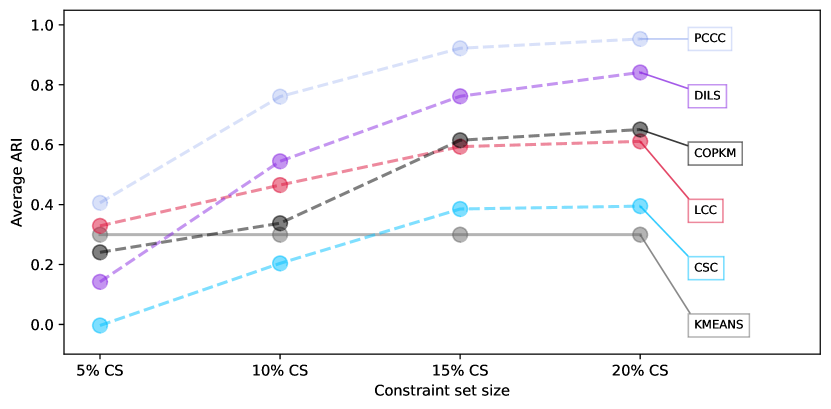
Figure 4: Adjusted Rand Index for different constraint set sizes, averaged across data sets (from collection COL1) and repetitions. Higher values indicate more overlap with the ground truth assignment. The PCCC algorithm consistently outperforms the state-of-the-art algorithms. Note that we replaced nan values with an ARI value of 0 before computing the averages.

Second, we compare the algorithms in terms of Silhouette coefficients. The higher the Silhouette coefficient of a solution, the better separated the clusters in the respective assignment. Figure 5 shows for each algorithm and for the different constraint set sizes, the Silhouette coefficients averaged across data sets and repetitions (random seeds). Note that we replaced nan values with a value of -1 before computing the averages. The solid green line in Figure 5 shows the Silhouette coefficient of the ground truth assignment. From Figure 5, we can see that the unconstrained KMEANS algorithm achieves the highest average Silhouette coefficients. The average Silhouette coefficients of the ground truth assignments are considerably lower than the Silhouette coefficients obtained by the KMEANS algorithm. This difference indicates that not all clusters in the ground truth assignment are homogeneous and well separated. Among the tested algorithms, the PCCC algorithm finds the best-separated clusters (highest Silhouette coefficients) for the constraint set sizes 5% CS and 10% CS. As the size of the constraint set increases, the Silhouette coefficients of the PCCC algorithm approach the Silhouette coefficients of the ground truth assignments. This behavior demonstrates that the constraint sets effectively guide the PCCC algorithm. The state-of-the-art algorithms generally obtain lower Silhouette coefficients except for the CSC algorithm for constraint set sizes 15% CS and 20% CS. Only the Silhouette coefficients of the DILS algorithm also approach the Silhouette coefficients of the ground truth assignment as the size of the constraint sets increases. Note that the average Silhouette coefficients of the LCC and the COPKM algorithms are considerably lower than the average scores of the other algorithms because they fail to return solutions for numerous instances. We report the detailed Silhouette coefficients for the individual data sets in the appendix in Tables 18–21.

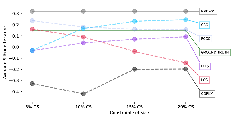
Figure 5: Silhouette coefficients for different constraint set sizes averaged across data sets (from collection COL1) and repetitions. High values indicate well-separated clusters. The PCCC algorithm achieves high Silhouette coefficients when the constraint sets are small. With larger constraint sets, the Silhouette coefficients obtained with the PCCC algorithm approach the Silhouette coefficients of the ground truth assignments, demonstrating that the algorithm effectively incorporates the constraints. The state-of-the-art algorithms achieve lower Silhouette coefficients (except CSC for 15% CS and 20% CS). Note that we replaced nan values with a Silhouette coefficient of -1 before computing the averages.

Finally, we compare the algorithms in terms of running time. Figure 6, which uses a logarithmic scale on the y-axis, compares the running times of the algorithms for the different constraint set sizes. The running times are averaged across repetitions and summed up across data sets. We replaced nan values with the time limit of 1,800 seconds before aggregating the results. The PCCC algorithm is considerably faster than the state-of-the-art approaches and slightly slower than the unconstrained KMEANS algorithm. In the appendix, we report the detailed running time results of all algorithms in Tables 22–25.

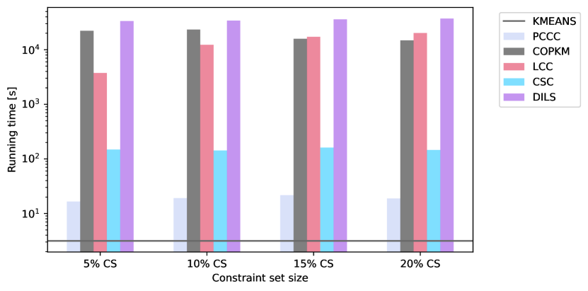
Figure 6: Running time in seconds for different constraint set sizes averaged across repetitions and summed up across data sets. The vertical axis uses a logarithmic scale. We replaced nan values with the time limit of 1,800 seconds before aggregating the results. The PCCC algorithm is considerably faster compared to the state-of-the-art approaches and only slightly slower than the unconstrained KMEANS algorithm.

5.5 Comparison to state-of-the-art approaches on synthetic data sets (COL2)

The comparison on synthetic data sets allows us to investigate the impact of two complexity parameters on the performance of the algorithms, namely the number of objects in a data set and the number of clusters to be identified. We use the same state-of-the-art algorithms and the same experimental design that we used for the comparison on benchmark data sets (see Section 5.4), except that we increased the time limit from 1,800 seconds to 3,600 seconds. We tested the following versions of the PCCC algorithm:

• PCCC: This is the baseline version that we used in the previous comparison. The pairwise constraints are provided as hard constraints. The model size reduction technique is not applied, i.e., model (MBLP) is solved in the assignment step of the algorithm with a solver time limit of 200 seconds. The initial positions of the cluster centers are determined with the k-means++ algorithm of Arthur and Vassilvitskii (2007). The algorithm uses the Gurobi Optimizer 9.5.2 as solver.

• PCCC-N2: This version corresponds to version PCCC with a potentially smaller model in the assignment step. To reduce the model size, we apply the reduction technique with $q=\max(2,\min(1+\Delta(H),k))$, i.e., parameter $q$ is set as small as possible, but larger than 2 and large enough such that we can still guarantee to find a feasible assignment, if one exists.

• PCCC-N2-S: In this version, we provide the must-link constraints as hard constraints and the cannot-link constraints as soft constraints with $w_{ij}=1$ for $\{i,j\}\in E^{\textup{SCL}}$. Moreover the model size reduction technique is applied with $q=2$, i.e., each object can only be assigned to one of the two closest clusters. Parameter $P$ is computed internally with the default procedure. Model (R($q$)MBLP) is solved with a solver time limit of 200 seconds. The initial positions of the cluster centers are determined with the k-means++ algorithm of Arthur and Vassilvitskii (2007). The algorithm uses the Gurobi Optimizer 9.5.2 as solver.

• PCCC-N3-S: Corresponds to PCCC-N2-S, but with $q=3$.

• PCCC-N5-S: Corresponds to PCCC-N2-S, but with $q=5$.

Figure 7 shows for each algorithm and for the different constraint set sizes, the ARI values averaged across data sets (from collection COL2) and repetitions (random seeds). Note that we replaced nan values with an ARI value of 0 before computing the averages. We noticed that the LCC algorithm stops with a runtime error when the constraint set is empty. This is why the LCC algorithm did not return any solutions for the constraint sets of size 0% CS. We can see that the highest average ARI values are achieved by the versions of the PCCC algorithm. Interestingly, the PCCC versions are the only algorithms that manage to outperform the unconstrained k-means algorithm on average. The low average ARI values of the DILS algorithm in this experiment are surprising. It turns out that the performance of the DILS algorithm strongly depends on the number of clusters to be identified. The larger the number of clusters, the lower the ARI values. Also the ARI values of the CSC and the LCC algorithm decrease when the number of clusters increases. While the different PCCC versions achieve similar ARI values for small constraint sets, the versions which treat the cannot-link constraints as soft constraints (PCCC-N2-S, PCCC-N3-S, and PCCC-N5-S), achieve slightly higher average ARI values for the large constraint sets. This is because the versions which treat the cannot-link constraints as hard constraints (PCCC, PCCC-N2) require considerable running time to find a feasible assignment when the number of cannot-link constraints is very large. The more detailed ARI results for the individual data sets are reported in the appendix in the Tables 26–30.

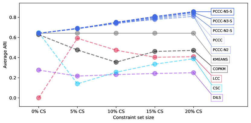
Figure 7: Adjusted Rand Index for different constraint set sizes, averaged across data sets (from collection COL2) and repetitions. Higher values indicate more overlap with the ground truth assignment. All versions of the PCCC algorithm consistently outperform the state-of-the-art algorithms. Note that we replaced nan values with an ARI value of 0 before computing the averages.

Figure 8 shows for each algorithm and for the different constraint set sizes, the Silhouette coefficients of all tested approaches averaged across data sets (from collection COL2) and repetitions. Note that we replaced nan values with a value of -1 before computing the averages. Figure 8 shows that the PCCC versions find better separated clusters than the state-of-the-art algorithms for all constraint set sizes. An interesting insight is that the CSC algorithm delivers higher Silhouette coefficients for the empty constraint sets than for the non-empty constraint sets. From looking at the Silhouette coefficients for the individual data sets that are presented in the appendix in Tables 31–35, we can see that the k-means style algorithms (all PCCC versions, the COPKM, and the LCC algorithm) tend to deliver higher Silhouette coefficients than the other algorithms (CSC and DILS), in particular when the number of clusters is large.

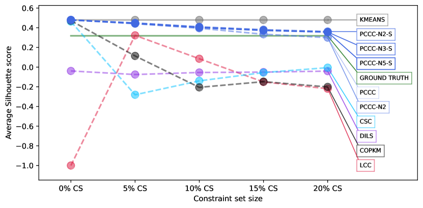
Figure 8: Silhouette coefficients for different constraint set sizes averaged across data sets (from collection COL2) and repetitions. High values indicate well-separated clusters. The PCCC versions achieve much higher Silhouette coefficients than the state-of-the-art algorithms when additional information is provided, i.e., when the constraint sets are non-empty. Note that we replaced nan values with a Silhouette coefficient of -1 before computing the averages.

Figure 9 visualizes the running time of the tested approaches on a logarithmic scale. We replaced nan values with the time limit of 3,600 seconds before aggregating the results. All versions of the PCCC algorithm are considerably faster than the state-of-the-art approaches. Also, the figure shows that the model-size reduction technique becomes highly effective when the cannot-link constraints are treated as soft constraints (see versions PCCC-N2-S, PCCC-N3-S, PCCC-N5-S). Version PCCC-N2, which treats the cannot-link constraints as hard constraints, performs almost identically as the baseline version (PCCC) with regards to both ARI and running time. This is because in version PCCC-N2, parameter $q$ is set such that a feasible assignment can be guaranteed if one exisits. It turns out that because of this requirement, parameter $q$ can rarely be set to a value smaller than the number of clusters $k$ leading to only moderate model size reductions. In the appendix, we report the detailed running time results of all algorithms in Tables 36–40.

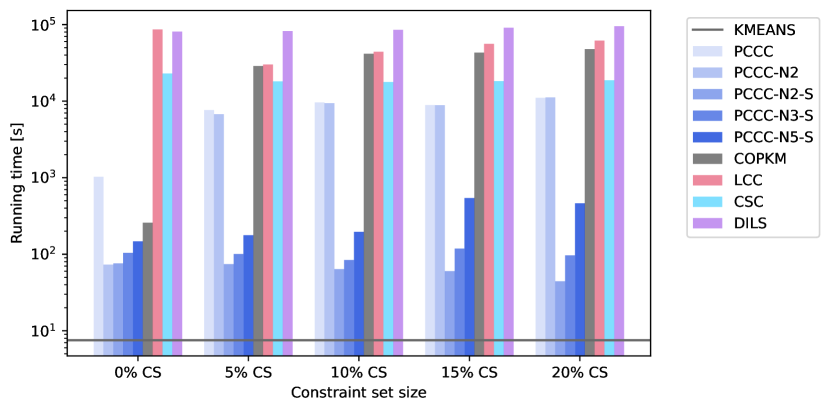
Figure 9: Running time in seconds for different constraint set sizes averaged across repetitions and summed up across data sets (from collection COL2). We replaced nan values with the time limit of 3,600 seconds before aggregating the results. The vertical axis uses a logarithmic scale. The PCCC versions (in particular those that treat the cannot-link constraints as soft constraints) are considerably faster compared to the state-of-the-art approaches.

To investigate for which type of instances the model-size reduction technique is particularly effective, we compared the performance of the baseline version (PCCC) to the performance of version PCCC-N5-S for different types of instances. Figure 10 visualizes the results of this comparison based on 10 heatmaps. The five heatmaps on the left analyze the absolute difference in ARI (ARI of PCCC-N5-S minus ARI of PCCC) for the five different constraint sets. The five heatmaps on the right analyze the speedup of version PCCC-N5-S over version PCCC (running time of PCCC divided by running time of PCCC-N5-S) for the five different constraint sets. Each heatmap has one entry for every synthetic data set. The entries are arranged such that the number of clusters increases from left to right and the number of objects increases from top to bottom. We can conclude that when the number of clusters is large (50 or more), the PCCC-N5-S version is considerably faster than the baseline version and delivers similar or sometimes even better ARI values.

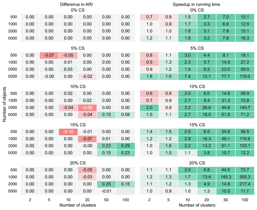
Figure 10: Comparison of baseline version PCCC with version PCCC-N5-S. The heatmaps on the left show the absolute difference in ARI (ARI of PCCC-N5-S minus ARI of PCCC) for the different instances and constraint set sizes, averaged across repetitions. The heatmaps on the right show the speedup (running time of PCCC divided by running time of PCCC-N5-S) of version PCCC-N5-S for the different instances and constraint set sizes. When the number of clusters is large (50 or more), the PCCC-N5-S version is considerably faster than the baseline version and delivers similar or substantially better ARI values.

5.6 Comparison to state-of-the-art approaches on large-sized data sets (COL3)

In this section, we conduct a third experiment with the large-sized data sets from collection COL3 that comprise up to 70,000 objects, 3,072 features, and 100 clusters to assess the scalability of the PCCC versions and the state-of-the-art approaches. We compared the PCCC versions introduced in the previous section to the state-of-the-art algorithms. The detailed results for the individual data sets are reported in the appendix in the Tables 41–52. It turns out that none of the state-of-the-art algorithms is able to return a solution for the Cifar 10 and Cifar 100 data sets, irrespective of the constraint sets used. Hence, the scalability of the state-of-the-art algorithms is limited. In contrast, the PCCC versions return solutions for all data sets and constraint sets, with the exception of versions PCCC and PCCC-N2, which fail to return a solution for data set Cifar 100 in combination with constraint set 5% CS. The constraint sets of the data set Cifar 100 contain much more cannot-link constraints than must-link constraints. Hence, for this data set the contraction of objects that are subject to a hard must-link constraint does not reduce the size of the input substantially. Nevertheless, the PCCC versions that treat the cannot-link constraints as soft constraints and use the model size reduction technique manage to produce solutions with considerably higher ARI values compared to the solutions obtained by the standard KMEANS algorithm. Figures 11, 12, and 13 visualize the aggregated ARI values, the aggregated Silhouette coefficients, and the aggregated running time results, respectively. Note that we replaced nan values with 0, -1 and the time limit of 3,600 seconds, respectively.

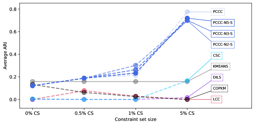
Figure 11: Adjusted Rand Index for different constraint set sizes, averaged across data sets (from collection COL3) and repetitions. Higher values indicate more overlap with the ground truth assignment. All versions of the PCCC algorithm consistently outperform the state-of-the-art algorithms. Note that we replaced nan values with an ARI value of 0 before computing the averages.

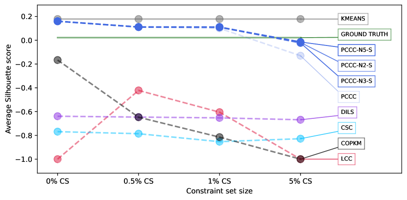
Figure 12: Silhouette coefficients for different constraint set sizes averaged across data sets (from collection COL3) and repetitions. High values indicate well-separated clusters. The PCCC versions achieve much higher average Silhouette coefficients than the state-of-the-art algorithms. Note that we replaced nan values with a Silhouette coefficient of -1 before computing the averages.

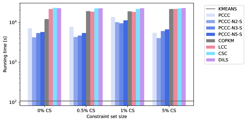
Figure 13: Running time in seconds for different constraint set sizes averaged across repetitions and summed up across data sets (from collection COL3). We replaced nan values with the time limit of 3,600 seconds before aggregating the results. The vertical axis uses a logarithmic scale. The PCCC versions are faster compared to the state-of-the-art approaches.

6 Constrained clustering with confidence values

Finally, we conduct a computational experiment to analyze the benefits of accounting for confidence values. For this analysis, we use the three small data sets Appendicitis, Moons, and Zoo, from collection COL1. With small data sets, the assignment problems of the PCCC versions can be solved optimally within a short running time. Hence, the reported results do not change if we increase the solver time limit. As described in Section 5.3, we generated 24 noisy constraint sets for each of the four data sets Appendicitis, Moons, and Zoo, resulting in 72 problem instances. From the state-of-the-art algorithms, only the CSC algorithm can take as input confidence values for the constraints. Therefore, the set of tested algorithms includes three versions of the PCCC algorithm, a version of the CSC algorithm, and the unconstrained KMEANS algorithm:

• PCCC: Corresponds to the baseline version that we used in the previous comparisons. The pairwise constraints are provided as hard constraints.

• PCCC-S: Corresponds to PCCC, but the pairwise constraints are provided as soft constraints with $w_{ij}=1$.

• PCCC-W: Corresponds to PCCC, but the pairwise constraints are provided as soft constraints and each constraint receives the confidence value $w_{ij}$ that was computed by the generation procedure described in Section 5.3.

• CSC-W: Corresponds to the CSC algorithm, but in this version of the algorithm, the constraint matrix $Q$ contains entry $w_{ij}$ for every noisy must-link constraint and entry $-w_{ij}$ for every noisy cannot-link constraint. All other settings are chosen as in version CSC.

• KMEANS: We set parameter n_init (number of initializations) to 1 and otherwise used the default settings.

We applied all algorithms three times to each problem instance, every time with a different random seed. Note that Gurobi solved all assignment problems of the PCCC versions to optimality within the time limit of 200 seconds. Figure 14 shows the ARI values obtained with the different algorithms averaged across data sets and repetitions for the different constraint sets. The figure contains a separate line plot for each of the four constraint set sizes, and the horizontal axes of the plots represent the amount of noise in the constraint sets (amount of noise decreases from left to right). Specifically, the horizontal axis represents the lower bound $l$ that was provided as an input parameter to the constraint set generation procedure. In the appendix, Tables 53–56 provide the detailed numerical results. When the noisy constraint sets are small (5% CS), the KMEANS and the PCCC versions deliver considerably better results than the state-of-the-art approach. For medium-sized constraint sets (10% CS), the soft version (PCCC-S) and the confidence-based version (PCCC-W) perform similarly well. Both versions outperform the version that treats the noisy constraints as hard constraints (PCCC) and the state-of-the-art approach (CSC-W), which both have substantially lower average ARI values compared to the KMEANS algorithm. For large-sized constraint sets (15% CS and 20% CS), the confidence-based variant (PCCC-W) consistently delivers the highest average ARI values compared to all other algorithms. The outperformance is substantial when the amount of noise is large, i.e., when the lower bound $l$ is low. These results demonstrate that accounting for confidence values is beneficial when the constraint sets are large and noisy. Another insight from Figure 14 is that it hurts performance to treat noisy constraints as hard constraints.

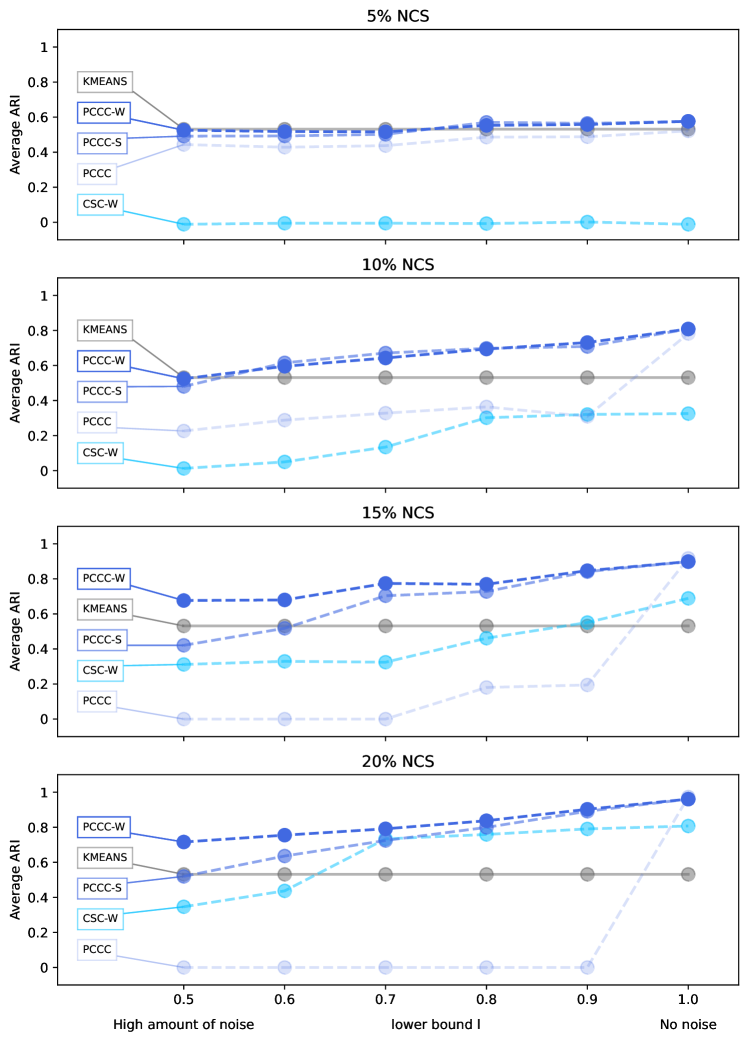
Figure 14: Adjusted Rand Index for different noisy constraint sets, averaged across data sets and repetitions. Higher values indicate more overlap with the ground truth assignment. Overall, the confidence-based variant (PCCC-W) delivers the highest ARI values, especially when the constraint sets are large and contain a high level of noise (amount of noise decreases from left to right).

7 Conclusions

In this paper, we introduce the PCCC algorithm for semi-supervised clustering. The PCCC algorithm is center-based and iterates between an object assignment and a cluster center update step. The key idea is to use integer programming to accommodate additional information in the form of constraints in the object assignment step. Using integer programming makes the algorithm more flexible than state-of-the-art algorithms. For example, the PCCC algorithm can accommodate the additional information in the form of hard or soft constraints, depending on the clustering application. Moreover, the user can specify a confidence value for each soft constraint that reflects the degree of belief in the corresponding information. We demonstrate that this flexibility is beneficial when the additional information is noisy. A key feature of the approach is a model size reduction technique based on kd-trees. This technique enables the algorithm to quickly generate high-quality solutions for instances with up to 60,000 objects, 3,072 features, 100 clusters, and hundreds of thousands of cannot-link constraints. In a comprehensive computational analysis, we demonstrate the superiority of the PCCC algorithm over the state-of-the-art approaches for semi-supervised clustering.

For future research, we plan to apply the proposed framework to related constrained clustering problems where the additional information is given in the form of cardinality, balance, or fairness constraints. Another promising research direction is using integer programming to incorporate additional information into density-based or graph-based clustering algorithms.

8 Acknowledgments

The research of the second author was supported in part by AI Institute NSF Award 2112533.

9 Appendix

	5% CS		10% CS		15% CS		20% CS
	ML	CL	ML	CL	ML	CL	ML	CL
Appendicitis	13	2	39	16	71	49	164	67
Breast Cancer	216	190	876	720	1,965	1,690	3,487	2,954
Bupa	79	74	323	272	699	627	1,201	1,145
Circles	50	55	208	227	502	488	853	917
Ecoli	30	106	163	398	357	918	609	1,669
Glass	11	44	52	179	139	389	259	644
Haberman	76	44	304	161	634	401	1,135	756
Hayesroth	12	16	39	81	102	174	177	319
Heart	41	50	178	173	396	424	744	687
Ionosphere	92	61	330	300	732	646	1,299	1,186
Iris	6	22	25	80	57	196	94	341
Led7Digit	25	275	126	1,099	267	2,508	460	4,490
Monk2	101	130	473	473	979	1,101	1,917	1,824
Moons	55	50	200	235	494	496	900	870
Movement Libras	6	147	27	603	112	1,319	158	2,398
Newthyroid	25	30	108	123	270	258	449	454
Saheart	152	124	595	486	1,292	1,123	2,330	1,948
Sonar	29	26	100	110	245	251	436	425
Spectfheart	56	35	233	118	543	277	965	466
Spiral	52	53	224	211	487	503	918	852
Soybean	0	3	4	6	6	22	12	33
Tae	8	20	40	80	82	171	151	314
Vehicle	221	682	874	2,696	1,955	6,046	3,589	10,776
Wine	8	28	31	122	70	281	143	487
Zoo	7	8	21	34	29	91	41	169

Table 11: Number of must-link (ML) and cannot-link (CL) constraints in the different constraint sets of collection COL1.

	5% CS		10% CS		15% CS		20% CS
	ML	CL	ML	CL	ML	CL	ML	CL
n500-k2	147	153	607	618	1,380	1,395	2,465	2,485
n500-k5	56	244	233	992	594	2,181	999	3,951
n500–k10	26	274	134	1,091	280	2,495	482	4,468
n500-k20	16	284	58	1,167	129	2,646	270	4,680
n500-k50	6	294	28	1,197	45	2,730	105	4,845
n500-k100	4	296	7	1,218	23	2,752	46	4,904
n1000-k2	607	618	2,494	2,456	5,559	5,616	10,007	9,893
n1000-k5	245	980	989	3,961	2,249	8,926	3,966	15,934
n1000-k10	127	1,098	449	4,501	1,119	10,056	1,996	17,904
n1000-k20	50	1,175	229	4,721	522	10,653	929	18,971
n1000-k50	26	1,199	91	4,859	203	10,972	404	19,496
n1000-k100	1	1,224	55	4,895	104	11,071	189	19,711
n2000-k2	2,472	2,478	9,984	9,916	22,405	22,445	39,612	40,188
n2000-k5	972	3,978	3,860	16,040	8,943	35,907	15,928	63,872
n2000-k10	472	4,478	1,978	17,922	4,405	40,445	7,950	71,850
n2000-k20	229	4,721	950	18,950	2,175	42,675	4,009	75,791
n2000-k50	90	4,860	363	19,537	860	43,990	1,594	78,206
n2000-k100	58	4,892	201	19,699	411	44,439	807	78,993
n5000-k2	15,632	15,493	62,161	62,589	140,016	140,859	249,040	250,460
n5000-k5	6,252	24,873	24,892	99,858	56,001	224,874	99,497	400,003
n5000-k10	3,106	28,019	12,458	112,292	27,954	252,921	49,307	450,193
n5000-k20	1,546	29,579	6,075	118,675	14,097	266,778	25,003	474,497
n5000-k50	607	30,518	2,440	122,310	5,536	275,339	9,762	489,738
n5000-k100	292	30,833	1,229	123,521	2,694	278,181	4,854	494,646

Table 12: Number of must-link (ML) and cannot-link (CL) constraints in the different constraint sets of collection COL2.

	0.5% CS		1% CS		5% CS
	ML	CL	ML	CL	ML	CL
Banana	160	191	707	671	17,797	17,183
Letter	190	4,760	743	19,157	19,165	480,335
Shuttle	27,099	14,806	108,254	59,656	2,707,873	1,495,677
Cifar 10	4,511	40,339	17,840	161,860	450,153	4,048,347
Cifar 100	467	44,383	1,760	177,940	44,792	4,453,708
Mnist	6,074	55,001	24,592	220,058	612,630	5,510,620

Table 13: Number of must-link (ML) and cannot-link (CL) constraints in the different constraint sets of collection COL3.

	5% CS
	PCCC	COPKM	CSC	DILS	LCC	KMEANS
Dataset
Appendicitis	0.467	0.182	-0.074	0.031	0.459	0.330
Breast Cancer	0.931	–	-0.001	0.568	0.655	0.675
Bupa	-0.000	–	-0.009	0.021	0.040	-0.005
Circles	0.001	–	0.001	0.163	0.015	-0.003
Ecoli	0.425	0.277	0.006	0.022	0.322	0.387
Glass	0.233	0.237	0.012	-0.025	0.226	0.239
Haberman	0.029	–	-0.037	0.006	0.004	0.094
Hayesroth	0.068	0.025	0.003	-0.015	0.122	0.062
Heart	0.600	–	0.002	0.227	0.617	0.407
Ionosphere	0.359	–	0.004	0.030	0.194	0.170
Iris	0.698	0.660	0.002	0.623	0.702	0.626
Led7Digit	0.456	0.407	-0.000	0.129	–	0.429
Monk2	0.715	–	-0.002	0.202	0.176	0.051
Moons	0.675	0.536	0.001	0.417	0.622	0.470
Movement Libras	0.296	0.307	-0.000	0.087	0.297	0.307
Newthyroid	0.790	0.779	-0.017	-0.071	0.789	0.593
Saheart	0.431	–	0.005	0.068	0.238	0.072
Sonar	0.012	–	0.001	0.040	0.088	0.005
Soybean	0.896	0.854	-0.000	0.183	0.723	0.896
Spectfheart	0.066	–	-0.043	0.236	0.023	-0.103
Spiral	0.074	–	0.002	0.107	0.079	0.027
Tae	0.055	0.024	-0.000	0.009	0.068	0.035
Vehicle	0.122	–	0.000	0.040	0.062	0.084
Wine	0.927	0.927	0.004	0.352	0.921	0.852
Zoo	0.826	0.804	0.052	0.117	0.783	0.794
Mean	0.406	0.241∗	-0.003	0.143	0.329∗	0.300

^∗Nan values (–) are replaced with 0 before computing the mean.

Table 14: Average Adjusted Rand Index (ARI) values of the PCCC algorithm and the four state-of-the-art algorithms (COPKM, CSC, DILS, LCC) obtained with constraint sets of size 5% CS. Higher values indicate more overlap with the ground truth assignment. The highest values are stated in bold. The column KMEANS reports the average ARI values that were obtained with the unconstrained k-means algorithm. The hyphen indicates that the respective algorithm returned no solution within the time limit of 1,800 seconds.

	10% CS
	PCCC	COPKM	CSC	DILS	LCC	KMEANS
Dataset
Appendicitis	0.60	–	-0.11	0.52	0.01	0.33
Breast Cancer	0.99	–	-0.00	1.00	0.79	0.67
Bupa	0.91	–	-0.01	0.95	0.68	-0.00
Circles	0.87	–	0.89	0.84	0.50	-0.00
Ecoli	0.69	0.50	0.10	0.13	0.61	0.39
Glass	0.21	0.19	0.03	0.02	0.26	0.24
Haberman	0.97	0.92	0.01	0.85	0.62	0.09
Hayesroth	0.15	–	0.04	0.04	0.10	0.06
Heart	0.89	–	0.02	0.88	0.09	0.41
Ionosphere	0.95	–	0.08	0.92	0.45	0.17
Iris	0.68	0.54	0.12	0.61	0.67	0.63
Led7Digit	0.68	0.52	0.01	0.11	0.56	0.43
Monk2	0.97	0.97	0.96	0.97	0.56	0.05
Moons	0.99	–	1.00	0.99	0.86	0.47
Movement Libras	0.32	0.30	0.01	0.08	0.32	0.31
Newthyroid	0.92	0.92	0.19	0.03	0.41	0.59
Saheart	0.98	0.97	0.73	0.97	0.64	0.07
Sonar	0.74	–	-0.00	0.63	0.09	0.00
Soybean	0.86	0.85	-0.03	0.21	0.61	0.90
Spectfheart	0.81	–	-0.02	0.97	0.59	-0.10
Spiral	0.87	–	0.21	0.84	0.44	0.03
Tae	0.15	–	0.01	0.02	0.05	0.03
Vehicle	0.96	–	0.49	0.30	–	0.08
Wine	0.93	0.93	0.22	0.58	0.85	0.85
Zoo	0.93	0.82	0.14	0.17	0.88	0.79
Mean	0.76	0.34∗	0.20	0.55	0.47∗	0.30

^∗Nan values (–) are replaced with 0 before computing the mean.

Table 15: Average Adjusted Rand Index (ARI) values of the PCCC algorithm and the four state-of-the-art algorithms (COPKM, CSC, DILS, LCC) obtained with constraint sets of size 10% CS. Higher values indicate more overlap with the ground truth assignment. The highest values are stated in bold. The column KMEANS reports the average ARI values that were obtained with the unconstrained k-means algorithm. The hyphen indicates that the respective algorithm returned no solution within the time limit of 1,800 seconds.

	15% CS
	PCCC	COPKM	CSC	DILS	LCC	KMEANS
Dataset
Appendicitis	1.00	–	0.97	0.73	0.05	0.33
Breast Cancer	1.00	1.00	0.00	1.00	1.00	0.67
Bupa	1.00	1.00	-0.01	1.00	0.99	-0.00
Circles	1.00	1.00	1.00	1.00	1.00	-0.00
Ecoli	0.93	–	0.24	0.62	0.80	0.39
Glass	0.79	–	0.01	0.38	0.45	0.24
Haberman	1.00	1.00	0.01	1.00	0.96	0.09
Hayesroth	0.98	–	0.11	0.51	0.44	0.06
Heart	1.00	1.00	0.65	1.00	0.83	0.41
Ionosphere	1.00	1.00	0.08	1.00	1.00	0.17
Iris	0.62	0.59	0.56	0.57	0.62	0.63
Led7Digit	0.88	–	0.01	0.11	–	0.43
Monk2	1.00	1.00	0.97	1.00	1.00	0.05
Moons	1.00	1.00	1.00	1.00	0.84	0.47
Movement Libras	0.33	0.30	0.02	0.07	0.32	0.31
Newthyroid	1.00	1.00	0.56	0.82	0.68	0.59
Saheart	1.00	1.00	0.78	1.00	–	0.07
Sonar	1.00	–	-0.00	1.00	0.78	0.00
Soybean	1.00	0.82	0.03	0.55	0.77	0.90
Spectfheart	1.00	0.98	-0.04	1.00	1.00	-0.10
Spiral	1.00	–	0.97	1.00	0.93	0.03
Tae	0.70	–	0.20	0.59	0.16	0.03
Vehicle	1.00	1.00	0.63	0.81	–	0.08
Wine	0.93	0.93	0.54	0.58	0.78	0.85
Zoo	0.89	0.75	0.33	0.71	0.92	0.79
Mean	0.92	0.61∗	0.39	0.76	0.65∗	0.30

^∗Nan values (–) are replaced with 0 before computing the mean.

Table 16: Average Adjusted Rand Index (ARI) values of the PCCC algorithm and the four state-of-the-art algorithms (COPKM, CSC, DILS, LCC) obtained with constraint sets of size 15% CS. Higher values indicate more overlap with the ground truth assignment. The highest values are stated in bold. The column KMEANS reports the average ARI values that were obtained with the unconstrained k-means algorithm. The hyphen indicates that the respective algorithm returned no solution within the time limit of 1,800 seconds.

	20% CS
	PCCC	COPKM	CSC	DILS	LCC	KMEANS
Dataset
Appendicitis	1.00	–	1.00	1.00	0.57	0.33
Breast Cancer	1.00	1.00	0.00	1.00	–	0.67
Bupa	1.00	1.00	-0.01	1.00	1.00	-0.00
Circles	1.00	1.00	1.00	1.00	–	-0.00
Ecoli	0.98	–	0.32	0.81	0.80	0.39
Glass	0.94	–	0.12	0.79	0.74	0.24
Haberman	1.00	1.00	0.01	1.00	1.00	0.09
Hayesroth	0.93	–	0.23	0.92	0.78	0.06
Heart	1.00	1.00	0.93	1.00	1.00	0.41
Ionosphere	1.00	1.00	0.05	1.00	–	0.17
Iris	0.65	0.60	0.56	0.57	0.63	0.63
Led7Digit	1.00	–	0.05	0.13	0.50	0.43
Monk2	1.00	1.00	0.89	1.00	–	0.05
Moons	1.00	1.00	0.96	1.00	1.00	0.47
Movement Libras	0.48	–	0.03	0.10	0.31	0.31
Newthyroid	1.00	0.98	0.86	1.00	0.85	0.59
Saheart	1.00	1.00	0.01	1.00	–	0.07
Sonar	1.00	1.00	-0.00	1.00	1.00	0.00
Soybean	1.00	1.00	0.13	0.70	0.79	0.90
Spectfheart	1.00	1.00	-0.01	1.00	1.00	-0.10
Spiral	1.00	–	1.00	1.00	1.00	0.03
Tae	0.96	–	0.36	0.94	0.54	0.03
Vehicle	1.00	1.00	0.30	0.82	–	0.08
Wine	0.96	0.95	0.73	0.61	0.90	0.85
Zoo	0.93	0.73	0.35	0.63	0.84	0.79
Mean	0.95	0.65∗	0.39	0.84	0.61∗	0.30

^∗Nan values (–) are replaced with 0 before computing the mean.

Table 17: Average Adjusted Rand Index (ARI) values of the PCCC algorithm and the four state-of-the-art algorithms (COPKM, CSC, DILS, LCC) obtained with constraint sets of size 20% CS. Higher values indicate more overlap with the ground truth assignment. The highest values are stated in bold. The column KMEANS reports the average ARI values that were obtained with the unconstrained k-means algorithm. The hyphen indicates that the respective algorithm returned no solution within the time limit of 1,800 seconds.

	5% CS
	PCCC	COPKM	CSC	DILS	LCC	KMEANS	GT
Dataset
Appendicitis	0.35	0.26	-0.05	-0.25	0.34	0.40	0.25
Breast Cancer	0.30	–	0.38	0.19	0.24	0.34	0.29
Bupa	0.15	–	-0.09	-0.02	0.14	0.45	0.00
Circles	0.17	–	0.20	-0.02	0.17	0.29	0.21
Ecoli	0.22	0.17	-0.27	-0.18	0.15	0.28	0.09
Glass	0.29	0.26	-0.35	-0.35	0.23	0.34	-0.03
Haberman	0.13	–	0.04	0.05	0.12	0.34	0.07
Hayesroth	0.16	0.14	-0.10	-0.15	0.17	0.21	0.01
Heart	0.13	–	0.34	0.07	0.13	0.16	0.11
Ionosphere	0.18	–	0.41	0.03	0.16	0.27	0.16
Iris	0.44	0.43	-0.25	0.35	0.44	0.46	0.38
Led7Digit	0.35	0.31	-0.11	-0.02	–	0.40	0.21
Monk2	0.09	–	-0.02	0.04	0.05	0.11	0.08
Moons	0.44	0.40	-0.09	0.32	0.38	0.50	0.38
Movement Libras	0.22	0.20	-0.30	-0.11	0.19	0.24	0.02
Newthyroid	0.51	0.52	-0.33	-0.36	0.51	0.60	0.46
Saheart	0.09	–	0.30	0.05	0.06	0.20	0.07
Sonar	0.13	–	0.32	-0.01	0.10	0.16	0.04
Soybean	0.34	0.32	-0.26	-0.07	0.23	0.34	0.36
Spectfheart	0.12	–	-0.05	-0.05	0.13	0.46	-0.08
Spiral	0.21	–	0.02	0.17	0.19	0.34	0.05
Tae	0.20	0.19	-0.16	-0.13	0.20	0.23	-0.02
Vehicle	0.04	–	0.04	-0.00	0.03	0.29	-0.01
Wine	0.28	0.28	-0.17	-0.02	0.28	0.28	0.28
Zoo	0.34	0.32	-0.20	-0.30	0.34	0.35	0.37
Mean	0.24	-0.33∗	-0.03	-0.03	0.16∗	0.32	0.15

^∗Nan values (–) are replaced with -1 before computing the mean.

Table 18: Average Silhouette coefficients of the PCCC algorithm and the four state-of-the-art algorithms (COPKM, CSC, DILS, LCC) obtained with constraint sets of size 5% CS. Higher values indicate better separated clusters. The highest values are stated in bold. The column KMEANS reports the average Silhouette coefficients that were obtained with the unconstrained k-means algorithm. The column GT reports the Silhouette coefficients of the ground truth assignment. The hyphen indicates that the respective algorithm returned no solution within the time limit of 1,800 seconds.

	10% CS
	PCCC	COPKM	CSC	DILS	LCC	KMEANS	GT
Dataset
Appendicitis	0.33	–	0.05	0.22	0.09	0.40	0.25
Breast Cancer	0.30	–	0.65	0.29	0.24	0.34	0.29
Bupa	0.01	–	0.61	0.00	0.01	0.45	0.00
Circles	0.18	–	0.21	0.15	0.14	0.29	0.21
Ecoli	0.15	0.10	-0.11	-0.14	0.12	0.28	0.09
Glass	0.08	0.03	0.17	-0.24	0.05	0.34	-0.03
Haberman	0.07	0.07	0.68	0.06	0.02	0.34	0.07
Hayesroth	0.07	–	-0.06	0.01	0.07	0.21	0.01
Heart	0.12	–	0.20	0.12	0.00	0.16	0.11
Ionosphere	0.17	–	0.36	0.15	0.12	0.27	0.16
Iris	0.45	0.40	0.22	0.25	0.45	0.46	0.38
Led7Digit	0.26	0.19	-0.06	-0.08	0.24	0.40	0.21
Monk2	0.08	0.08	0.08	0.08	0.04	0.11	0.08
Moons	0.38	–	0.38	0.38	0.39	0.50	0.38
Movement Libras	0.19	0.15	-0.13	-0.10	0.17	0.24	0.02
Newthyroid	0.48	0.48	0.06	-0.09	0.19	0.60	0.46
Saheart	0.07	0.07	0.10	0.07	0.04	0.20	0.07
Sonar	0.04	–	0.39	0.03	0.02	0.16	0.04
Soybean	0.34	0.32	-0.21	-0.01	0.20	0.34	0.36
Spectfheart	-0.05	–	0.55	-0.08	-0.06	0.46	-0.08
Spiral	0.06	–	0.03	0.06	0.03	0.34	0.05
Tae	0.10	–	-0.01	0.03	0.05	0.23	-0.02
Vehicle	-0.01	–	-0.01	-0.03	–	0.29	-0.01
Wine	0.29	0.29	0.08	0.07	0.28	0.28	0.28
Zoo	0.35	0.31	-0.06	-0.27	0.35	0.35	0.37
Mean	0.18	-0.42∗	0.17	0.04	0.09∗	0.32	0.15

^∗Nan values (–) are replaced with -1 before computing the mean.

Table 19: Average Silhouette coefficients of the PCCC algorithm and the four state-of-the-art algorithms (COPKM, CSC, DILS, LCC) obtained with constraint sets of size 10% CS. Higher values indicate better separated clusters. The highest values are stated in bold. The column KMEANS reports the average Silhouette coefficients that were obtained with the unconstrained k-means algorithm. The column GT reports the Silhouette coefficients of the ground truth assignment. The hyphen indicates that the respective algorithm returned no solution within the time limit of 1,800 seconds.

	15% CS
	PCCC	COPKM	CSC	DILS	LCC	KMEANS	GT
Dataset
Appendicitis	0.25	–	0.24	0.19	0.04	0.40	0.25
Breast Cancer	0.29	0.29	0.66	0.29	0.29	0.34	0.29
Bupa	0.00	0.00	0.62	0.00	0.00	0.45	0.00
Circles	0.21	0.21	0.21	0.21	0.21	0.29	0.21
Ecoli	0.16	–	-0.10	-0.04	0.13	0.28	0.09
Glass	0.02	–	0.24	-0.23	-0.03	0.34	-0.03
Haberman	0.07	0.07	0.68	0.07	0.07	0.34	0.07
Hayesroth	0.01	–	0.01	-0.05	-0.00	0.21	0.01
Heart	0.11	0.11	0.19	0.11	0.09	0.16	0.11
Ionosphere	0.16	0.16	0.36	0.16	0.16	0.27	0.16
Iris	0.46	0.43	0.49	0.24	0.46	0.46	0.38
Led7Digit	0.24	–	-0.03	-0.09	–	0.40	0.21
Monk2	0.08	0.08	0.09	0.08	0.08	0.11	0.08
Moons	0.38	0.38	0.38	0.38	0.31	0.50	0.38
Movement Libras	0.06	0.03	-0.11	-0.12	0.06	0.24	0.02
Newthyroid	0.46	0.46	0.49	0.36	0.35	0.60	0.46
Saheart	0.07	0.07	0.11	0.07	–	0.20	0.07
Sonar	0.04	–	0.39	0.04	0.02	0.16	0.04
Soybean	0.36	0.31	-0.04	0.15	0.23	0.34	0.36
Spectfheart	-0.08	-0.08	0.54	-0.08	-0.08	0.46	-0.08
Spiral	0.05	–	0.05	0.05	0.04	0.34	0.05
Tae	-0.00	–	0.08	-0.02	-0.02	0.23	-0.02
Vehicle	-0.01	-0.01	-0.01	-0.02	–	0.29	-0.01
Wine	0.29	0.29	0.24	0.09	0.27	0.28	0.28
Zoo	0.33	0.23	-0.02	-0.12	0.35	0.35	0.37
Mean	0.16	-0.20∗	0.23	0.07	0.00∗	0.32	0.15

^∗Nan values (–) are replaced with -1 before computing the mean.

Table 20: Average Silhouette coefficients of the PCCC algorithm and the four state-of-the-art algorithms (COPKM, CSC, DILS, LCC) obtained with constraint sets of size 15% CS. Higher values indicate better separated clusters. The highest values are stated in bold. The column KMEANS reports the average Silhouette coefficients that were obtained with the unconstrained k-means algorithm. The column GT reports the Silhouette coefficients of the ground truth assignment. The hyphen indicates that the respective algorithm returned no solution within the time limit of 1,800 seconds.

	20% CS
	PCCC	COPKM	CSC	DILS	LCC	KMEANS	GT
Dataset
Appendicitis	0.25	–	0.25	0.25	0.14	0.40	0.25
Breast Cancer	0.29	0.29	0.66	0.29	–	0.34	0.29
Bupa	0.00	0.00	0.63	0.00	0.00	0.45	0.00
Circles	0.21	0.21	0.21	0.21	–	0.29	0.21
Ecoli	0.16	–	-0.07	0.04	0.08	0.28	0.09
Glass	0.01	–	0.04	-0.09	0.03	0.34	-0.03
Haberman	0.07	0.07	0.68	0.07	0.07	0.34	0.07
Hayesroth	0.01	–	0.11	0.01	0.01	0.21	0.01
Heart	0.11	0.11	0.12	0.11	0.11	0.16	0.11
Ionosphere	0.16	0.16	0.38	0.16	–	0.27	0.16
Iris	0.45	0.43	0.50	0.24	0.45	0.46	0.38
Led7Digit	0.21	–	-0.04	-0.08	0.00	0.40	0.21
Monk2	0.08	0.08	0.09	0.08	–	0.11	0.08
Moons	0.38	0.38	0.40	0.38	0.38	0.50	0.38
Movement Libras	0.01	–	-0.11	-0.11	-0.02	0.24	0.02
Newthyroid	0.46	0.47	0.38	0.46	0.43	0.60	0.46
Saheart	0.07	0.07	0.44	0.07	–	0.20	0.07
Sonar	0.04	0.04	0.39	0.04	0.04	0.16	0.04
Soybean	0.36	0.36	-0.01	0.13	0.24	0.34	0.36
Spectfheart	-0.08	-0.08	0.58	-0.08	-0.08	0.46	-0.08
Spiral	0.05	–	0.05	0.05	0.05	0.34	0.05
Tae	-0.02	–	0.09	-0.02	-0.03	0.23	-0.02
Vehicle	-0.01	-0.01	0.05	-0.02	–	0.29	-0.01
Wine	0.28	0.28	0.24	0.11	0.28	0.28	0.28
Zoo	0.34	0.22	0.06	0.01	0.29	0.35	0.37
Mean	0.16	-0.20∗	0.25	0.09	-0.14∗	0.32	0.15

^∗Nan values (–) are replaced with -1 before computing the mean.

Table 21: Average Silhouette coefficients of the PCCC algorithm and the four state-of-the-art algorithms (COPKM, CSC, DILS, LCC) obtained with constraint sets of size 20% CS. Higher values indicate better separated clusters. The highest values are stated in bold. The column KMEANS reports the average Silhouette coefficients that were obtained with the unconstrained k-means algorithm. The column GT reports the Silhouette coefficients of the ground truth assignment. The hyphen indicates that the respective algorithm returned no solution within the time limit of 1,800 seconds.

	5% CS
	PCCC	COPKM	CSC	DILS	LCC	KMEANS
Dataset
Appendicitis	0.1	0.0	5.1	501.4	6.4	0.2
Breast Cancer	0.3	–	5.3	1,818.9	104.4	0.2
Bupa	0.4	–	2.6	1,658.8	18.9	0.2
Circles	0.1	–	1.8	1,346.8	8.6	0.1
Ecoli	1.4	0.4	2.0	1,447.1	41.9	0.1
Glass	0.4	0.2	1.7	969.1	28.9	0.2
Haberman	0.4	–	4.4	1,331.1	9.2	0.2
Hayesroth	0.3	0.0	1.7	716.5	7.3	0.2
Heart	0.6	–	4.1	1,391.3	22.4	0.2
Ionosphere	0.4	–	5.8	1,810.6	71.3	0.2
Iris	0.6	0.0	6.4	615.5	6.2	0.3
Led7Digit	1.4	0.4	6.1	1,810.3	–	0.2
Monk2	0.7	–	4.9	1,801.8	23.6	0.1
Moons	0.3	0.0	9.0	1,259.3	6.3	0.2
Movement Libras	2.1	5.9	7.5	1,809.3	853.1	0.3
Newthyroid	0.5	0.0	4.0	980.6	11.0	0.2
Saheart	0.6	–	8.1	1,811.1	39.0	0.2
Sonar	0.5	–	5.8	1,480.5	73.0	0.2
Soybean	0.3	0.0	1.6	229.7	17.2	0.2
Spectfheart	0.4	–	6.8	1,809.9	64.6	0.2
Spiral	0.4	–	4.2	1,280.8	7.7	0.3
Tae	0.4	0.0	2.8	670.0	8.7	0.2
Vehicle	2.2	–	15.3	1,826.6	274.1	0.1
Wine	0.2	0.1	5.3	906.4	17.7	0.2
Zoo	0.5	0.1	1.4	456.4	23.4	0.3
Sum	15.8	21,607.3∗	123.5	31,739.7	3,545.2∗	5.0

^∗Nan values (–) are replaced with 1,800 before computing the sum.

Table 22: Average running times (in seconds) of the PCCC algorithm and the four state-of-the-art algorithms (COPKM, CSC, DILS, LCC) for the constraint sets of size 5% CS. The lowest values are stated in bold. The column KMEANS reports the average running time of the unconstrained k-means algorithm. The hyphen indicates that the respective algorithm returned no solution within the time limit of 1,800 seconds.

	10% CS
	PCCC	COPKM	CSC	DILS	LCC	KMEANS
Dataset
Appendicitis	0.2	–	1.5	488.8	7.4	0.2
Breast Cancer	0.2	–	6.9	1,808.1	445.1	0.2
Bupa	0.3	–	4.4	1,795.4	224.0	0.1
Circles	0.2	–	2.9	1,397.8	246.7	0.2
Ecoli	1.5	0.4	5.1	1,525.9	34.6	0.2
Glass	0.8	1.9	5.3	972.2	42.8	0.2
Haberman	0.2	0.1	2.7	1,456.0	176.9	0.2
Hayesroth	0.4	–	2.7	734.2	11.7	0.2
Heart	0.1	–	7.4	1,464.7	117.9	0.3
Ionosphere	0.3	–	4.4	1,809.2	1,815.1	0.2
Iris	0.5	0.0	3.8	647.8	6.8	0.2
Led7Digit	3.4	0.5	4.9	1,808.5	107.0	0.2
Monk2	0.2	3.3	3.3	1,809.3	631.6	0.2
Moons	0.3	–	4.6	1,396.1	46.1	0.2
Movement Libras	5.3	6.3	4.9	1,806.2	1,007.9	0.3
Newthyroid	0.4	0.1	2.2	977.6	21.6	0.2
Saheart	0.2	2.7	7.0	1,812.8	852.4	0.2
Sonar	0.3	–	3.6	1,516.7	269.5	0.2
Soybean	0.2	0.0	1.0	246.6	16.4	0.2
Spectfheart	0.3	–	5.1	1,809.2	267.0	0.2
Spiral	0.2	–	4.7	1,396.3	188.0	0.2
Tae	0.5	–	3.7	696.7	11.5	0.3
Vehicle	0.7	–	14.3	1,811.9	–	0.2
Wine	0.3	0.1	3.5	912.2	19.5	0.2
Zoo	0.4	0.1	1.4	481.9	19.1	0.3
Sum	17.4	23,415.6∗	111.5	32,581.7	8,386.6∗	5.3

^∗Nan values (–) are replaced with 1,800 before computing the sum.

Table 23: Average running times (in seconds) of the PCCC algorithm and the four state-of-the-art algorithms (COPKM, CSC, DILS, LCC) for the constraint sets of size 10% CS. The lowest values are stated in bold. The column KMEANS reports the average running time of the unconstrained k-means algorithm. The hyphen indicates that the respective algorithm returned no solution within the time limit of 1,800 seconds.

	15% CS
	PCCC	COPKM	CSC	DILS	LCC	KMEANS
Dataset
Appendicitis	0.2	–	5.3	567.2	16.7	0.2
Breast Cancer	0.1	36.1	5.5	1,815.7	27.6	0.2
Bupa	0.1	6.4	2.2	1,805.8	1,953.1	0.2
Circles	0.1	2.8	5.2	1,552.0	1,850.0	0.3
Ecoli	1.2	–	8.0	1,787.9	238.9	0.2
Glass	0.7	–	1.9	1,090.4	537.3	0.2
Haberman	0.1	1.7	10.7	1,705.6	167.4	0.2
Hayesroth	0.3	–	3.4	782.7	59.2	0.2
Heart	0.3	1.9	5.1	1,625.7	501.0	0.2
Ionosphere	0.2	5.0	2.0	1,807.2	809.4	0.2
Iris	0.6	0.0	7.6	759.5	9.5	0.3
Led7Digit	5.4	–	12.2	1,817.7	–	0.2
Monk2	0.3	15.2	8.3	1,811.8	6.6	0.2
Moons	0.1	2.8	5.4	1,568.5	46.7	0.2
Movement Libras	7.7	8.8	7.9	1,815.2	1,513.9	0.2
Newthyroid	0.1	0.1	6.1	1,114.6	192.6	0.2
Saheart	0.3	15.5	5.9	1,816.4	–	0.2
Sonar	0.4	–	7.3	1,605.9	1,433.7	0.2
Soybean	0.1	0.0	0.9	236.1	19.4	0.2
Spectfheart	0.4	6.5	6.8	1,812.0	531.7	0.2
Spiral	0.1	–	5.5	1,626.3	91.5	0.2
Tae	0.5	–	1.9	797.8	83.3	0.2
Vehicle	0.4	92.7	16.9	1,847.4	–	0.2
Wine	0.4	0.1	3.7	1,027.0	63.1	0.2
Zoo	0.6	0.1	6.0	508.5	20.4	0.2
Sum	20.6	14,595.9∗	151.4	34,704.9	15,573.0∗	5.2

^∗Nan values (–) are replaced with 1,800 before computing the sum.

Table 24: Average running times (in seconds) of the PCCC algorithm and the four state-of-the-art algorithms (COPKM, CSC, DILS, LCC) for the constraint sets of size 15% CS. The lowest values are stated in bold. The column KMEANS reports the average running time of the unconstrained k-means algorithm. The hyphen indicates that the respective algorithm returned no solution within the time limit of 1,800 seconds.

	20% CS
	PCCC	COPKM	CSC	DILS	LCC	KMEANS
Dataset
Appendicitis	0.2	–	4.4	606.1	42.8	0.3
Breast Cancer	0.4	65.7	5.4	1,847.9	–	0.2
Bupa	0.2	11.4	3.5	1,811.6	5.5	0.2
Circles	0.3	6.3	4.9	1,807.2	–	0.3
Ecoli	0.7	–	7.3	1,806.4	1,360.9	0.2
Glass	0.4	–	1.7	1,239.5	1,018.3	0.2
Haberman	0.3	4.3	8.7	1,803.4	7.4	0.2
Hayesroth	0.1	–	6.4	865.3	68.4	0.2
Heart	0.2	4.3	7.2	1,810.7	6.2	0.3
Ionosphere	0.3	10.3	2.6	1,815.9	–	0.2
Iris	0.4	0.0	5.4	814.4	16.7	0.3
Led7Digit	2.3	–	5.0	1,826.6	1,843.0	0.3
Monk2	0.5	24.5	5.9	1,818.8	–	0.3
Moons	0.1	6.3	4.0	1,804.3	2.9	0.2
Movement Libras	10.0	–	6.1	1,815.9	1,850.7	0.3
Newthyroid	0.3	0.2	2.8	1,357.8	546.0	0.2
Saheart	0.4	28.1	6.2	1,817.4	–	0.2
Sonar	0.4	1.5	6.6	1,777.1	19.5	0.4
Soybean	0.4	0.0	2.2	243.8	29.0	0.3
Spectfheart	0.3	7.9	5.7	1,815.4	760.2	0.2
Spiral	0.5	–	4.8	1,811.0	7.5	0.2
Tae	0.3	–	5.9	835.5	693.2	0.2
Vehicle	0.4	157.0	14.0	1,840.1	–	0.4
Wine	0.4	0.1	6.5	1,115.9	658.8	0.2
Zoo	0.5	0.1	3.9	539.5	28.5	0.2
Sum	20.1	14,728.0∗	137.2	36,647.4	19,765.6∗	6.3

^∗Nan values (–) are replaced with 1,800 before computing the sum.

Table 25: Average running times (in seconds) of the PCCC algorithm and the four state-of-the-art algorithms (COPKM, CSC, DILS, LCC) for the constraint sets of size 20% CS. The lowest values are stated in bold. The column KMEANS reports the average running time of the unconstrained k-means algorithm. The hyphen indicates that the respective algorithm returned no solution within the time limit of 1,800 seconds.

	0% CS
	PCCC	PCCC-N2	PCCC-N2-S	PCCC-N3-S	PCCC-N5-S	COPKM	CSC	DILS	LCC	KMEANS
Dataset
n500-k2	0.960	0.960	0.960	0.960	0.960	0.968	1.000	0.992	–	0.968
n500-k5	0.774	0.774	0.774	0.774	0.774	0.766	0.866	0.782	–	0.773
n500–k10	0.874	0.874	0.874	0.874	0.874	0.775	0.897	0.458	–	0.874
n500-k20	0.562	0.562	0.562	0.562	0.562	0.529	0.500	0.155	–	0.563
n500-k50	0.376	0.376	0.376	0.376	0.376	0.394	0.355	0.037	–	0.376
n500-k100	0.221	0.221	0.221	0.221	0.221	0.209	0.205	0.009	–	0.221
n1000-k2	0.984	0.984	0.984	0.984	0.984	0.984	1.000	1.000	–	0.984
n1000-k5	0.857	0.857	0.857	0.857	0.857	0.764	0.855	0.623	–	0.860
n1000-k10	0.801	0.801	0.801	0.801	0.801	0.772	0.896	0.294	–	0.801
n1000-k20	0.574	0.574	0.574	0.574	0.574	0.573	0.519	0.097	–	0.574
n1000-k50	0.398	0.398	0.398	0.398	0.398	0.399	0.391	0.022	–	0.398
n1000-k100	0.238	0.238	0.238	0.238	0.238	0.237	0.235	0.007	–	0.238
n2000-k2	0.966	0.966	0.966	0.966	0.966	0.965	0.994	0.990	–	0.963
n2000-k5	0.771	0.771	0.771	0.771	0.771	0.867	0.865	0.330	–	0.770
n2000-k10	0.835	0.835	0.835	0.835	0.835	0.751	0.867	0.127	–	0.835
n2000-k20	0.588	0.588	0.588	0.588	0.588	0.588	0.549	0.038	–	0.589
n2000-k50	0.407	0.407	0.407	0.407	0.407	0.412	0.391	0.009	–	0.406
n2000-k100	0.246	0.246	0.246	0.246	0.246	0.241	0.240	0.005	–	0.246
n5000-k2	0.985	0.985	0.985	0.985	0.985	0.985	1.000	0.554	–	0.985
n5000-k5	0.865	0.865	0.865	0.865	0.865	0.816	0.865	0.063	–	0.866
n5000-k10	0.856	0.856	0.856	0.856	0.856	0.859	0.874	0.021	–	0.855
n5000-k20	0.587	0.587	0.587	0.587	0.587	0.572	0.539	0.006	–	0.593
n5000-k50	0.421	0.421	0.421	0.421	0.421	0.413	0.394	0.002	–	0.421
n5000-k100	0.248	0.248	0.248	0.248	0.248	0.244	0.238	0.001	–	0.248
Mean	0.641	0.641	0.641	0.641	0.641	0.628	0.647	0.276	0.000∗	0.642

^∗Nan values (–) are replaced with 0 before computing the mean.

Table 26: Average Adjusted Rand Index (ARI) values of five versions of the PCCC algorithm and the four state-of-the-art algorithms (COPKM, CSC, DILS, LCC) obtained with constraint sets of size 0% CS. Higher values indicate more overlap with the ground truth assignment. The highest values are stated in bold. The column KMEANS reports the average ARI values that were obtained with the unconstrained k-means algorithm. The hyphen indicates that the respective algorithm returned no solution within the time limit of 1,800 seconds. We noticed that the LCC algorithm stops with a runtime error when the constraint set is empty. This is why the LCC algorithm did not return any solutions for the constraint sets of size 0% CS.

	5% CS
	PCCC	PCCC-N2	PCCC-N2-S	PCCC-N3-S	PCCC-N5-S	COPKM	CSC	DILS	LCC	KMEANS
Dataset
n500-k2	0.99	0.99	0.99	0.99	0.99	–	0.00	0.95	1.00	0.97
n500-k5	0.91	0.91	0.85	0.85	0.84	0.79	0.00	0.58	0.74	0.77
n500–k10	0.90	0.90	0.86	0.86	0.85	0.75	0.00	0.24	0.83	0.87
n500-k20	0.56	0.56	0.56	0.56	0.56	0.52	0.00	0.12	0.52	0.56
n500-k50	0.38	0.38	0.38	0.38	0.38	0.39	0.00	0.03	0.37	0.38
n500-k100	0.21	0.21	0.21	0.21	0.21	0.21	0.01	0.02	0.22	0.22
n1000-k2	1.00	1.00	1.00	1.00	1.00	1.00	1.00	0.99	1.00	0.98
n1000-k5	0.93	0.93	0.93	0.93	0.93	–	0.00	0.40	0.84	0.86
n1000-k10	0.89	0.89	0.90	0.90	0.90	0.85	0.00	0.17	0.72	0.80
n1000-k20	0.61	0.61	0.61	0.61	0.61	0.59	0.00	0.06	0.55	0.57
n1000-k50	0.42	0.42	0.42	0.42	0.42	0.39	0.00	0.02	0.42	0.40
n1000-k100	0.24	0.24	0.24	0.24	0.24	0.24	0.00	0.01	–	0.24
n2000-k2	1.00	1.00	1.00	1.00	1.00	1.00	1.00	1.00	0.51	0.96
n2000-k5	0.95	0.95	0.95	0.95	0.95	0.95	0.01	0.11	0.78	0.77
n2000-k10	0.84	0.84	0.88	0.88	0.86	0.88	0.00	0.05	0.85	0.83
n2000-k20	0.64	0.64	0.64	0.65	0.64	0.58	0.00	0.02	0.62	0.59
n2000-k50	0.41	0.41	0.42	0.42	0.42	0.40	0.00	0.01	0.44	0.41
n2000-k100	0.25	0.25	0.25	0.25	0.25	0.24	0.00	0.00	0.26	0.25
n5000-k2	1.00	1.00	1.00	1.00	1.00	–	1.00	0.42	0.93	0.98
n5000-k5	1.00	1.00	1.00	1.00	1.00	0.97	0.32	0.00	0.88	0.87
n5000-k10	0.98	0.98	0.98	0.98	0.98	–	0.00	0.00	0.48	0.86
n5000-k20	0.76	0.76	0.71	0.70	0.74	–	0.00	0.00	0.54	0.59
n5000-k50	0.48	0.48	0.49	0.48	0.48	0.42	0.00	0.00	0.46	0.42
n5000-k100	0.25	0.25	0.25	0.25	0.25	0.25	0.00	0.00	0.26	0.25
Mean	0.69	0.69	0.69	0.69	0.69	0.48∗	0.14	0.22	0.59∗	0.64

^∗Nan values (–) are replaced with 0 before computing the mean.

Table 27: Average Adjusted Rand Index (ARI) values of five versions of the PCCC algorithm and the four state-of-the-art algorithms (COPKM, CSC, DILS, LCC) obtained with constraint sets of size 5% CS. Higher values indicate more overlap with the ground truth assignment. The highest values are stated in bold. The column KMEANS reports the average ARI values that were obtained with the unconstrained k-means algorithm. The hyphen indicates that the respective algorithm returned no solution within the time limit of 3,600 seconds.

	10% CS
	PCCC	PCCC-N2	PCCC-N2-S	PCCC-N3-S	PCCC-N5-S	COPKM	CSC	DILS	LCC	KMEANS
Dataset
n500-k2	1.00	1.00	1.00	1.00	1.00	1.00	1.00	1.00	0.53	0.97
n500-k5	0.97	0.97	0.97	0.97	0.97	–	0.03	0.77	0.92	0.77
n500–k10	0.90	0.90	0.92	0.91	0.91	0.81	0.01	0.24	0.77	0.87
n500-k20	0.61	0.61	0.62	0.61	0.61	0.54	0.00	0.08	0.52	0.56
n500-k50	0.39	0.39	0.39	0.39	0.39	0.38	0.00	0.03	0.40	0.38
n500-k100	0.22	0.22	0.22	0.22	0.22	0.22	0.00	0.01	0.22	0.22
n1000-k2	1.00	1.00	1.00	1.00	1.00	1.00	1.00	1.00	0.67	0.98
n1000-k5	0.99	0.99	0.83	0.99	0.99	0.96	0.20	0.64	0.88	0.86
n1000-k10	0.98	0.98	0.94	0.94	0.98	–	0.01	0.09	0.77	0.80
n1000-k20	0.68	0.68	0.67	0.71	0.70	–	0.00	0.04	0.50	0.57
n1000-k50	0.43	0.43	0.43	0.43	0.43	0.40	0.00	0.02	0.41	0.40
n1000-k100	0.26	0.26	0.26	0.26	0.26	0.25	0.00	0.01	0.25	0.24
n2000-k2	1.00	1.00	1.00	1.00	1.00	1.00	1.00	1.00	1.00	0.96
n2000-k5	1.00	1.00	1.00	1.00	1.00	1.00	0.71	0.20	0.94	0.77
n2000-k10	0.99	0.99	0.95	0.95	0.95	–	0.03	0.01	0.64	0.83
n2000-k20	0.90	0.90	0.81	0.82	0.82	–	0.01	0.01	0.51	0.59
n2000-k50	0.49	0.49	0.51	0.50	0.49	0.41	0.01	0.01	0.46	0.41
n2000-k100	0.27	0.27	0.27	0.27	0.27	0.25	0.00	0.00	0.27	0.25
n5000-k2	1.00	1.00	1.00	1.00	1.00	–	1.00	0.40	–	0.98
n5000-k5	1.00	1.00	1.00	1.00	1.00	–	0.73	0.00	–	0.87
n5000-k10	1.00	1.00	0.96	1.00	1.00	–	0.32	0.00	–	0.86
n5000-k20	0.98	0.98	0.89	0.89	0.94	–	0.03	0.00	–	0.59
n5000-k50	0.56	0.56	0.70	0.71	0.71	–	0.01	0.00	0.41	0.42
n5000-k100	0.27	0.27	0.34	0.35	0.35	0.27	0.01	0.00	0.29	0.25
Mean	0.75	0.75	0.74	0.75	0.75	0.35∗	0.26	0.23	0.47∗	0.64

^∗Nan values (–) are replaced with 0 before computing the mean.

Table 28: Average Adjusted Rand Index (ARI) values of five versions of the PCCC algorithm and the four state-of-the-art algorithms (COPKM, CSC, DILS, LCC) obtained with constraint sets of size 10% CS. Higher values indicate more overlap with the ground truth assignment. The highest values are stated in bold. The column KMEANS reports the average ARI values that were obtained with the unconstrained k-means algorithm. The hyphen indicates that the respective algorithm returned no solution within the time limit of 3,600 seconds.

	15% CS
	PCCC	PCCC-N2	PCCC-N2-S	PCCC-N3-S	PCCC-N5-S	COPKM	CSC	DILS	LCC	KMEANS
Dataset
n500-k2	1.00	1.00	1.00	1.00	1.00	1.00	1.00	1.00	1.00	0.97
n500-k5	0.99	0.99	0.92	0.91	0.99	0.99	0.43	0.88	0.92	0.77
n500–k10	0.98	0.98	0.90	0.90	0.88	–	0.03	0.32	0.94	0.87
n500-k20	0.71	0.71	0.71	0.70	0.70	0.54	0.01	0.08	0.56	0.56
n500-k50	0.43	0.43	0.43	0.43	0.43	0.40	0.00	0.03	0.41	0.38
n500-k100	0.24	0.24	0.24	0.24	0.24	0.22	0.01	0.02	0.25	0.22
n1000-k2	1.00	1.00	1.00	1.00	1.00	1.00	1.00	1.00	–	0.98
n1000-k5	1.00	1.00	0.85	1.00	1.00	1.00	0.72	0.68	0.99	0.86
n1000-k10	0.99	0.99	0.99	0.99	0.99	1.00	0.07	0.09	0.71	0.80
n1000-k20	0.89	0.89	0.81	0.81	0.82	–	0.01	0.02	0.48	0.57
n1000-k50	0.51	0.51	0.51	0.50	0.52	0.41	0.01	0.01	0.46	0.40
n1000-k100	0.28	0.28	0.28	0.28	0.28	0.27	0.00	0.01	0.28	0.24
n2000-k2	1.00	1.00	1.00	1.00	1.00	–	1.00	1.00	–	0.96
n2000-k5	1.00	1.00	1.00	1.00	1.00	1.00	0.73	0.23	1.00	0.77
n2000-k10	1.00	1.00	1.00	1.00	1.00	1.00	0.40	0.02	–	0.83
n2000-k20	0.98	0.98	0.90	0.92	0.98	0.95	0.03	0.01	0.60	0.59
n2000-k50	0.46	0.46	0.66	0.68	0.68	–	0.01	0.00	0.44	0.41
n2000-k100	0.04	0.04	0.34	0.33	0.33	0.29	0.01	0.00	0.30	0.25
n5000-k2	1.00	1.00	1.00	1.00	1.00	–	1.00	0.39	–	0.98
n5000-k5	1.00	1.00	1.00	1.00	1.00	–	0.73	0.01	–	0.87
n5000-k10	1.00	1.00	1.00	1.00	1.00	–	0.74	0.00	–	0.86
n5000-k20	1.00	1.00	0.92	0.92	1.00	1.00	0.08	0.00	–	0.59
n5000-k50	0.75	0.75	0.84	0.88	0.90	–	0.02	0.00	–	0.42
n5000-k100	0.40	0.40	0.57	0.61	0.63	–	0.01	0.00	0.34	0.25
Mean	0.78	0.78	0.79	0.80	0.81	0.46∗	0.33	0.24	0.40∗	0.64

^∗Nan values (–) are replaced with 0 before computing the mean.

Table 29: Average Adjusted Rand Index (ARI) values of five versions of the PCCC algorithm and the four state-of-the-art algorithms (COPKM, CSC, DILS, LCC) obtained with constraint sets of size 15% CS. Higher values indicate more overlap with the ground truth assignment. The highest values are stated in bold. The column KMEANS reports the average ARI values that were obtained with the unconstrained k-means algorithm. The hyphen indicates that the respective algorithm returned no solution within the time limit of 3,600 seconds.

	20% CS
	PCCC	PCCC-N2	PCCC-N2-S	PCCC-N3-S	PCCC-N5-S	COPKM	CSC	DILS	LCC	KMEANS
Dataset
n500-k2	1.00	1.00	1.00	1.00	1.00	1.00	1.00	1.00	1.00	0.97
n500-k5	1.00	1.00	1.00	1.00	1.00	1.00	0.68	0.90	0.99	0.77
n500–k10	0.99	0.99	0.99	0.99	0.99	0.97	0.07	0.44	0.73	0.87
n500-k20	0.85	0.85	0.76	0.78	0.80	–	0.02	0.08	0.61	0.56
n500-k50	0.48	0.48	0.46	0.48	0.48	0.45	0.01	0.04	0.43	0.38
n500-k100	0.26	0.26	0.25	0.25	0.25	0.24	0.01	0.02	0.26	0.22
n1000-k2	1.00	1.00	1.00	1.00	1.00	1.00	1.00	1.00	–	0.98
n1000-k5	1.00	1.00	1.00	1.00	1.00	1.00	0.73	0.67	1.00	0.86
n1000-k10	1.00	1.00	1.00	1.00	1.00	1.00	0.36	0.15	0.87	0.80
n1000-k20	0.96	0.96	0.87	0.89	0.93	–	0.03	0.02	0.63	0.57
n1000-k50	0.67	0.67	0.62	0.66	0.67	–	0.01	0.01	0.46	0.40
n1000-k100	0.32	0.32	0.32	0.32	0.32	0.30	0.01	0.01	0.30	0.24
n2000-k2	1.00	1.00	1.00	1.00	1.00	–	1.00	1.00	–	0.96
n2000-k5	1.00	1.00	1.00	1.00	1.00	1.00	0.73	0.21	–	0.77
n2000-k10	1.00	1.00	0.93	1.00	1.00	1.00	0.76	0.02	0.93	0.83
n2000-k20	1.00	1.00	0.89	0.96	1.00	1.00	0.04	0.00	0.72	0.59
n2000-k50	0.57	0.57	0.77	0.80	0.82	–	0.02	0.00	0.53	0.41
n2000-k100	0.35	0.35	0.46	0.48	0.49	0.38	0.01	0.00	0.35	0.25
n5000-k2	1.00	1.00	1.00	1.00	1.00	–	1.00	0.41	–	0.98
n5000-k5	1.00	1.00	1.00	1.00	1.00	–	0.82	0.01	–	0.87
n5000-k10	1.00	1.00	1.00	1.00	1.00	–	0.75	0.00	–	0.86
n5000-k20	1.00	1.00	0.95	1.00	1.00	–	0.24	0.00	–	0.59
n5000-k50	0.99	0.99	0.93	0.95	0.99	0.99	0.02	0.00	–	0.42
n5000-k100	–	–	0.75	0.78	0.81	–	0.02	0.00	–	0.25
Mean	0.81∗	0.81∗	0.83	0.85	0.86	0.47∗	0.39	0.25	0.41∗	0.64

^∗Nan values (–) are replaced with 0 before computing the mean.

Table 30: Average Adjusted Rand Index (ARI) values of five versions of the PCCC algorithm and the four state-of-the-art algorithms (COPKM, CSC, DILS, LCC) obtained with constraint sets of size 20% CS. Higher values indicate more overlap with the ground truth assignment. The highest values are stated in bold. The column KMEANS reports the average ARI values that were obtained with the unconstrained k-means algorithm. The hyphen indicates that the respective algorithm returned no solution within the time limit of 3,600 seconds.

	0% CS
	PCCC	PCCC-N2	PCCC-N2-S	PCCC-N3-S	PCCC-N5-S	COPKM	CSC	DILS	LCC	KMEANS	GT
Dataset
n500-k2	0.54	0.54	0.54	0.54	0.54	0.54	0.54	0.54	–	0.54	0.54
n500-k5	0.70	0.70	0.70	0.70	0.70	0.70	0.67	0.58	–	0.70	0.61
n500–k10	0.56	0.56	0.56	0.56	0.56	0.50	0.54	0.10	–	0.56	0.50
n500-k20	0.39	0.39	0.39	0.39	0.39	0.38	0.36	-0.17	–	0.39	0.21
n500-k50	0.37	0.37	0.37	0.37	0.37	0.37	0.34	-0.45	–	0.37	0.07
n500-k100	0.37	0.37	0.37	0.37	0.37	0.34	0.33	-0.65	–	0.37	-0.11
n1000-k2	0.54	0.54	0.54	0.54	0.54	0.54	0.54	0.54	–	0.54	0.54
n1000-k5	0.66	0.66	0.66	0.66	0.66	0.69	0.66	0.38	–	0.66	0.60
n1000-k10	0.55	0.55	0.55	0.55	0.55	0.54	0.55	-0.01	–	0.55	0.51
n1000-k20	0.39	0.39	0.39	0.39	0.39	0.38	0.35	-0.19	–	0.39	0.24
n1000-k50	0.36	0.36	0.36	0.36	0.36	0.36	0.34	-0.36	–	0.36	0.10
n1000-k100	0.37	0.37	0.37	0.37	0.37	0.35	0.34	-0.47	–	0.37	-0.06
n2000-k2	0.55	0.55	0.55	0.55	0.55	0.55	0.55	0.55	–	0.55	0.55
n2000-k5	0.70	0.70	0.70	0.70	0.70	0.67	0.67	0.08	–	0.70	0.60
n2000-k10	0.55	0.55	0.55	0.55	0.55	0.54	0.56	-0.12	–	0.55	0.51
n2000-k20	0.39	0.39	0.39	0.39	0.39	0.38	0.35	-0.20	–	0.39	0.24
n2000-k50	0.35	0.35	0.35	0.35	0.35	0.36	0.34	-0.29	–	0.35	0.10
n2000-k100	0.34	0.34	0.34	0.34	0.34	0.33	0.34	-0.35	–	0.34	-0.05
n5000-k2	0.54	0.54	0.54	0.54	0.54	0.54	0.54	0.33	–	0.54	0.54
n5000-k5	0.67	0.67	0.67	0.67	0.67	0.68	0.67	-0.10	–	0.67	0.60
n5000-k10	0.57	0.57	0.57	0.57	0.57	0.54	0.55	-0.13	–	0.57	0.51
n5000-k20	0.38	0.38	0.38	0.38	0.38	0.38	0.34	-0.14	–	0.38	0.23
n5000-k50	0.35	0.35	0.35	0.35	0.35	0.34	0.32	-0.16	–	0.35	0.10
n5000-k100	0.34	0.34	0.34	0.34	0.34	0.33	0.32	-0.23	–	0.34	-0.05
Mean	0.48	0.48	0.48	0.48	0.48	0.47	0.46	-0.04	-1.00∗	0.48	0.32

^∗Nan values (–) are replaced with -1 before computing the mean.

Table 31: Average Silhouette coefficients of five versions of the PCCC algorithm and the four state-of-the-art algorithms (COPKM, CSC, DILS, LCC) obtained with constraint sets of size 0% CS. Higher values indicate better separated clusters. The highest values are stated in bold. The column KMEANS reports the average Silhouette coefficients that were obtained with the unconstrained k-means algorithm. The column GT reports the Silhouette coefficients of the ground truth assignment. The hyphen indicates that the respective algorithm returned no solution within the time limit of 3,600 seconds. We noticed that the LCC algorithm stops with a runtime error when the constraint set is empty. This is why the LCC algorithm did not return any solutions for the constraint sets of size 0% CS.

	5% CS
	PCCC	PCCC-N2	PCCC-N2-S	PCCC-N3-S	PCCC-N5-S	COPKM	CSC	DILS	LCC	KMEANS	GT
Dataset
n500-k2	0.54	0.54	0.54	0.54	0.54	–	-0.15	0.51	0.54	0.54	0.54
n500-k5	0.65	0.65	0.66	0.66	0.64	0.60	-0.17	0.32	0.49	0.70	0.61
n500–k10	0.53	0.53	0.56	0.56	0.55	0.45	-0.41	-0.07	0.52	0.56	0.50
n500-k20	0.39	0.39	0.39	0.39	0.39	0.36	-0.53	-0.21	0.35	0.39	0.21
n500-k50	0.37	0.37	0.37	0.37	0.37	0.36	-0.72	-0.45	0.35	0.37	0.07
n500-k100	0.34	0.34	0.34	0.34	0.34	0.32	-0.73	-0.64	0.31	0.37	-0.11
n1000-k2	0.54	0.54	0.54	0.54	0.54	0.54	0.54	0.53	0.54	0.54	0.54
n1000-k5	0.63	0.63	0.63	0.63	0.63	–	-0.45	0.13	0.59	0.66	0.60
n1000-k10	0.53	0.53	0.55	0.55	0.54	0.50	-0.34	-0.11	0.44	0.55	0.51
n1000-k20	0.36	0.36	0.36	0.36	0.36	0.35	-0.37	-0.23	0.33	0.39	0.24
n1000-k50	0.34	0.34	0.34	0.34	0.34	0.32	-0.70	-0.33	0.34	0.36	0.10
n1000-k100	0.36	0.36	0.36	0.36	0.36	0.34	-0.77	-0.47	–	0.37	-0.06
n2000-k2	0.55	0.55	0.55	0.55	0.55	0.55	0.55	0.55	0.29	0.55	0.55
n2000-k5	0.62	0.62	0.62	0.62	0.62	0.62	-0.23	-0.09	0.51	0.70	0.60
n2000-k10	0.48	0.48	0.56	0.55	0.53	0.49	-0.31	-0.16	0.48	0.55	0.51
n2000-k20	0.32	0.32	0.32	0.32	0.32	0.29	-0.30	-0.19	0.32	0.39	0.24
n2000-k50	0.31	0.31	0.31	0.31	0.31	0.30	-0.57	-0.26	0.32	0.35	0.10
n2000-k100	0.31	0.31	0.31	0.30	0.31	0.30	-0.78	-0.33	0.24	0.34	-0.05
n5000-k2	0.54	0.54	0.54	0.54	0.54	–	0.54	0.25	0.51	0.54	0.54
n5000-k5	0.61	0.61	0.61	0.61	0.61	0.59	0.14	-0.06	0.54	0.67	0.60
n5000-k10	0.51	0.51	0.51	0.51	0.51	–	-0.10	-0.06	0.07	0.57	0.51
n5000-k20	0.27	0.27	0.28	0.26	0.27	–	-0.13	-0.10	0.18	0.38	0.23
n5000-k50	0.26	0.26	0.27	0.26	0.26	0.22	-0.22	-0.14	0.25	0.35	0.10
n5000-k100	0.26	0.26	0.26	0.26	0.26	0.24	-0.54	-0.20	0.25	0.34	-0.05
Mean	0.44	0.44	0.45	0.45	0.44	0.11∗	-0.28	-0.08	0.32∗	0.48	0.32

^∗Nan values (–) are replaced with -1 before computing the mean.

Table 32: Average Silhouette coefficients of five versions of the PCCC algorithm and the four state-of-the-art algorithms (COPKM, CSC, DILS, LCC) obtained with constraint sets of size 5% CS. Higher values indicate better separated clusters. The highest values are stated in bold. The column KMEANS reports the average Silhouette coefficients that were obtained with the unconstrained k-means algorithm. The column GT reports the Silhouette coefficients of the ground truth assignment. The hyphen indicates that the respective algorithm returned no solution within the time limit of 3,600 seconds.

	10% CS
	PCCC	PCCC-N2	PCCC-N2-S	PCCC-N3-S	PCCC-N5-S	COPKM	CSC	DILS	LCC	KMEANS	GT
Dataset
n500-k2	0.54	0.54	0.54	0.54	0.54	0.54	0.54	0.54	0.30	0.54	0.54
n500-k5	0.62	0.62	0.62	0.62	0.62	–	-0.24	0.42	0.62	0.70	0.61
n500–k10	0.50	0.50	0.53	0.53	0.53	0.44	-0.34	-0.06	0.40	0.56	0.50
n500-k20	0.33	0.33	0.34	0.33	0.33	0.30	-0.43	-0.26	0.29	0.39	0.21
n500-k50	0.33	0.33	0.33	0.33	0.33	0.29	-0.67	-0.42	0.27	0.37	0.07
n500-k100	0.34	0.34	0.34	0.34	0.34	0.30	-0.74	-0.65	0.27	0.37	-0.11
n1000-k2	0.54	0.54	0.54	0.54	0.54	0.54	0.54	0.54	0.33	0.54	0.54
n1000-k5	0.60	0.60	0.62	0.60	0.60	0.58	-0.16	0.29	0.53	0.66	0.60
n1000-k10	0.52	0.52	0.53	0.52	0.52	–	-0.16	-0.16	0.38	0.55	0.51
n1000-k20	0.28	0.28	0.29	0.29	0.28	–	-0.33	-0.22	0.20	0.39	0.24
n1000-k50	0.28	0.28	0.29	0.28	0.28	0.26	-0.64	-0.33	0.26	0.36	0.10
n1000-k100	0.29	0.29	0.30	0.29	0.29	0.27	-0.73	-0.44	0.26	0.37	-0.06
n2000-k2	0.55	0.55	0.55	0.55	0.55	0.55	0.55	0.55	0.55	0.55	0.55
n2000-k5	0.61	0.61	0.61	0.61	0.61	0.61	0.62	-0.03	0.57	0.70	0.60
n2000-k10	0.51	0.51	0.52	0.52	0.51	–	-0.22	-0.12	0.18	0.55	0.51
n2000-k20	0.27	0.27	0.26	0.25	0.24	–	-0.17	-0.18	0.10	0.39	0.24
n2000-k50	0.21	0.21	0.24	0.22	0.22	0.17	-0.32	-0.24	0.21	0.35	0.10
n2000-k100	0.23	0.23	0.24	0.23	0.23	0.19	-0.60	-0.32	0.22	0.34	-0.05
n5000-k2	0.54	0.54	0.54	0.54	0.54	–	0.54	0.24	–	0.54	0.54
n5000-k5	0.60	0.60	0.60	0.60	0.60	–	0.63	-0.04	–	0.67	0.60
n5000-k10	0.51	0.51	0.50	0.51	0.51	–	-0.18	-0.05	–	0.57	0.51
n5000-k20	0.24	0.24	0.23	0.23	0.22	–	-0.18	-0.07	–	0.38	0.23
n5000-k50	0.03	0.03	0.15	0.14	0.14	–	-0.24	-0.12	0.02	0.35	0.10
n5000-k100	0.03	0.03	0.12	0.10	0.10	0.03	-0.44	-0.18	0.08	0.34	-0.05
Mean	0.40	0.40	0.41	0.40	0.40	-0.21∗	-0.14	-0.05	0.08∗	0.48	0.32

^∗Nan values (–) are replaced with -1 before computing the mean.

Table 33: Average Silhouette coefficients of five versions of the PCCC algorithm and the four state-of-the-art algorithms (COPKM, CSC, DILS, LCC) obtained with constraint sets of size 10% CS. Higher values indicate better separated clusters. The highest values are stated in bold. The column KMEANS reports the average Silhouette coefficients that were obtained with the unconstrained k-means algorithm. The column GT reports the Silhouette coefficients of the ground truth assignment. The hyphen indicates that the respective algorithm returned no solution within the time limit of 3,600 seconds.

	15% CS
	PCCC	PCCC-N2	PCCC-N2-S	PCCC-N3-S	PCCC-N5-S	COPKM	CSC	DILS	LCC	KMEANS	GT
Dataset
n500-k2	0.54	0.54	0.54	0.54	0.54	0.54	0.54	0.54	0.54	0.54	0.54
n500-k5	0.62	0.62	0.64	0.62	0.62	0.62	0.05	0.50	0.56	0.70	0.61
n500–k10	0.50	0.50	0.53	0.53	0.50	–	-0.22	-0.04	0.49	0.56	0.50
n500-k20	0.26	0.26	0.26	0.26	0.26	0.18	-0.29	-0.24	0.22	0.39	0.21
n500-k50	0.27	0.27	0.28	0.28	0.28	0.25	-0.64	-0.45	0.25	0.37	0.07
n500-k100	0.28	0.28	0.29	0.28	0.28	0.25	-0.72	-0.66	0.25	0.37	-0.11
n1000-k2	0.54	0.54	0.54	0.54	0.54	0.54	0.54	0.54	–	0.54	0.54
n1000-k5	0.60	0.60	0.62	0.60	0.60	0.60	0.63	0.31	0.59	0.66	0.60
n1000-k10	0.51	0.51	0.51	0.51	0.51	0.51	-0.23	-0.16	0.29	0.55	0.51
n1000-k20	0.26	0.26	0.25	0.25	0.24	–	-0.23	-0.21	0.06	0.39	0.24
n1000-k50	0.20	0.20	0.22	0.21	0.21	0.12	-0.50	-0.33	0.19	0.36	0.10
n1000-k100	0.24	0.24	0.25	0.24	0.24	0.19	-0.69	-0.49	0.22	0.37	-0.06
n2000-k2	0.55	0.55	0.55	0.55	0.55	–	0.55	0.55	–	0.55	0.55
n2000-k5	0.60	0.60	0.60	0.60	0.60	0.60	0.64	-0.01	0.60	0.70	0.60
n2000-k10	0.51	0.51	0.51	0.51	0.51	0.51	0.02	-0.13	–	0.55	0.51
n2000-k20	0.25	0.25	0.25	0.24	0.25	0.23	-0.19	-0.14	0.02	0.39	0.24
n2000-k50	-0.05	-0.05	0.15	0.14	0.14	–	-0.34	-0.20	0.06	0.35	0.10
n2000-k100	-0.30	-0.30	0.14	0.14	0.13	0.07	-0.55	-0.32	0.11	0.34	-0.05
n5000-k2	0.54	0.54	0.54	0.54	0.54	–	0.54	0.24	–	0.54	0.54
n5000-k5	0.60	0.60	0.60	0.60	0.60	–	0.63	-0.06	–	0.67	0.60
n5000-k10	0.51	0.51	0.51	0.51	0.51	–	0.25	-0.06	–	0.57	0.51
n5000-k20	0.23	0.23	0.21	0.21	0.23	0.23	-0.37	-0.06	–	0.38	0.23
n5000-k50	-0.06	-0.06	0.11	0.10	0.10	–	-0.29	-0.12	–	0.35	0.10
n5000-k100	-0.19	-0.19	0.01	-0.00	-0.01	–	-0.45	-0.19	-0.08	0.34	-0.05
Mean	0.33	0.33	0.38	0.38	0.37	-0.15∗	-0.06	-0.05	-0.15∗	0.48	0.32

^∗Nan values (–) are replaced with -1 before computing the mean.

Table 34: Average Silhouette coefficients of five versions of the PCCC algorithm and the four state-of-the-art algorithms (COPKM, CSC, DILS, LCC) obtained with constraint sets of size 15% CS. Higher values indicate better separated clusters. The highest values are stated in bold. The column KMEANS reports the average Silhouette coefficients that were obtained with the unconstrained k-means algorithm. The column GT reports the Silhouette coefficients of the ground truth assignment. The hyphen indicates that the respective algorithm returned no solution within the time limit of 3,600 seconds.

	20% CS
	PCCC	PCCC-N2	PCCC-N2-S	PCCC-N3-S	PCCC-N5-S	COPKM	CSC	DILS	LCC	KMEANS	GT
Dataset
n500-k2	0.54	0.54	0.54	0.54	0.54	0.54	0.54	0.54	0.54	0.54	0.54
n500-k5	0.61	0.61	0.61	0.61	0.61	0.61	0.58	0.51	0.61	0.70	0.61
n500–k10	0.50	0.50	0.50	0.50	0.50	0.50	-0.21	0.04	0.29	0.56	0.50
n500-k20	0.26	0.26	0.26	0.26	0.25	–	-0.34	-0.26	0.15	0.39	0.21
n500-k50	0.22	0.22	0.23	0.23	0.22	0.16	-0.59	-0.43	0.19	0.37	0.07
n500-k100	0.23	0.23	0.24	0.23	0.23	0.18	-0.70	-0.63	0.19	0.37	-0.11
n1000-k2	0.54	0.54	0.54	0.54	0.54	0.54	0.54	0.54	–	0.54	0.54
n1000-k5	0.60	0.60	0.60	0.60	0.60	0.60	0.64	0.30	0.60	0.66	0.60
n1000-k10	0.51	0.51	0.51	0.51	0.51	0.51	-0.06	-0.11	0.38	0.55	0.51
n1000-k20	0.25	0.25	0.24	0.23	0.24	–	-0.24	-0.20	0.08	0.39	0.24
n1000-k50	0.15	0.15	0.17	0.16	0.15	–	-0.45	-0.30	0.10	0.36	0.10
n1000-k100	0.16	0.16	0.18	0.17	0.16	0.11	-0.64	-0.45	0.13	0.37	-0.06
n2000-k2	0.55	0.55	0.55	0.55	0.55	–	0.55	0.55	–	0.55	0.55
n2000-k5	0.60	0.60	0.60	0.60	0.60	0.60	0.64	-0.04	–	0.70	0.60
n2000-k10	0.51	0.51	0.55	0.51	0.51	0.51	0.33	-0.15	0.44	0.55	0.51
n2000-k20	0.24	0.24	0.23	0.23	0.24	0.24	-0.27	-0.13	0.04	0.39	0.24
n2000-k50	-0.18	-0.18	0.11	0.10	0.09	–	-0.30	-0.21	-0.01	0.35	0.10
n2000-k100	-0.09	-0.09	0.06	0.05	0.04	-0.04	-0.57	-0.30	0.01	0.34	-0.05
n5000-k2	0.54	0.54	0.54	0.54	0.54	–	0.54	0.25	–	0.54	0.54
n5000-k5	0.60	0.60	0.60	0.60	0.60	–	0.62	-0.07	–	0.67	0.60
n5000-k10	0.51	0.51	0.51	0.51	0.51	–	0.26	-0.06	–	0.57	0.51
n5000-k20	0.23	0.23	0.23	0.23	0.23	–	-0.28	-0.07	–	0.38	0.23
n5000-k50	0.10	0.10	0.10	0.10	0.11	0.10	-0.30	-0.12	–	0.35	0.10
n5000-k100	–	–	-0.03	-0.04	-0.04	–	-0.43	-0.16	–	0.34	-0.05
Mean	0.30∗	0.30∗	0.36	0.36	0.36	-0.20∗	-0.01	-0.04	-0.22∗	0.48	0.32

^∗Nan values (–) are replaced with -1 before computing the mean.

Table 35: Average Silhouette coefficients of five versions of the PCCC algorithm and the four state-of-the-art algorithms (COPKM, CSC, DILS, LCC) obtained with constraint sets of size 20% CS. Higher values indicate better separated clusters. The highest values are stated in bold. The column KMEANS reports the average Silhouette coefficients that were obtained with the unconstrained k-means algorithm. The column GT reports the Silhouette coefficients of the ground truth assignment. The hyphen indicates that the respective algorithm returned no solution within the time limit of 3,600 seconds.

	0% CS
	PCCC	PCCC-N2	PCCC-N2-S	PCCC-N3-S	PCCC-N5-S	COPKM	CSC	DILS	LCC	KMEANS
Dataset
n500-k2	0.3	0.6	0.3	0.4	0.4	0.1	2.7	2,718.1	–	0.3
n500-k5	0.6	0.5	0.5	0.6	0.7	0.1	2.9	2,459.8	–	0.2
n500–k10	1.5	0.5	0.5	0.7	1.0	0.3	3.2	2,414.0	–	0.5
n500-k20	4.3	0.8	0.9	1.1	1.6	0.6	3.0	2,484.1	–	0.3
n500-k50	7.7	0.6	0.6	1.0	1.1	2.6	11.0	2,313.2	–	0.2
n500-k100	11.0	1.2	0.6	0.7	1.1	8.7	4.2	2,307.5	–	0.5
n1000-k2	0.8	0.7	0.8	0.7	0.8	0.1	25.0	3,639.8	–	0.2
n1000-k5	2.0	1.3	1.2	1.7	2.3	0.2	27.8	3,614.3	–	0.2
n1000-k10	3.4	0.9	1.1	1.6	2.0	0.6	27.1	3,614.5	–	0.2
n1000-k20	8.3	1.7	1.5	2.0	2.5	1.7	31.5	3,618.3	–	0.2
n1000-k50	24.4	1.9	1.8	2.6	3.6	5.7	32.1	3,614.9	–	0.2
n1000-k100	26.8	1.8	1.4	1.6	2.1	18.3	34.1	3,617.5	–	0.6
n2000-k2	1.3	1.5	1.4	1.4	1.3	0.2	243.1	3,682.0	–	0.2
n2000-k5	4.0	2.5	2.3	3.0	4.2	0.4	258.7	3,675.7	–	0.4
n2000-k10	8.4	2.2	2.4	3.2	4.6	1.2	259.6	3,651.8	–	0.4
n2000-k20	18.0	3.2	2.9	4.3	5.8	3.8	262.5	3,609.1	–	0.5
n2000-k50	59.4	3.8	4.0	5.4	7.6	11.9	268.8	3,663.2	–	0.5
n2000-k100	77.7	2.6	2.8	3.8	5.1	39.9	271.6	3,631.1	–	0.6
n5000-k2	3.6	2.7	3.0	3.0	3.0	0.7	3,269.0	3,869.5	–	0.5
n5000-k5	9.9	4.3	4.8	6.1	9.2	1.4	3,462.1	3,771.3	–	0.5
n5000-k10	14.8	3.7	4.1	5.3	8.0	3.3	3,682.9	3,746.6	–	0.4
n5000-k20	81.2	10.9	11.6	17.3	25.4	9.8	3,633.0	3,685.8	–	0.9
n5000-k50	200.9	11.4	12.2	17.7	25.9	41.3	3,499.3	3,718.3	–	0.9
n5000-k100	458.2	11.9	13.1	19.0	28.1	105.8	3,609.3	3,731.3	–	1.1
Sum	1,028.7	73.2	75.9	104.2	147.6	258.5	22,924.5	80,851.8	86,400.0∗	10.6

^∗Nan values (–) are replaced with 3,600 before computing the sum.

Table 36: Average running times (in seconds) of five versions of the PCCC algorithm and the four state-of-the-art algorithms (COPKM, CSC, DILS, LCC) for the constraint sets of size 0% CS. The lowest values are stated in bold. The column KMEANS reports the average running time of the unconstrained k-means algorithm. The hyphen indicates that the respective algorithm returned no solution within the time limit of 3,600 seconds. We noticed that the LCC algorithm stops with a runtime error when the constraint set is empty. This is why the LCC algorithm did not return any solutions for the constraint sets of size 0% CS.

	5% CS
	PCCC	PCCC-N2	PCCC-N2-S	PCCC-N3-S	PCCC-N5-S	COPKM	CSC	DILS	LCC	KMEANS
Dataset
n500-k2	0.4	0.5	0.5	0.5	0.7	–	2.9	3,039.7	8.2	0.3
n500-k5	1.4	1.4	0.7	0.9	1.3	0.1	2.9	2,506.3	20.2	0.1
n500–k10	3.3	2.0	0.6	0.8	1.1	0.3	2.7	2,549.4	28.7	0.1
n500-k20	8.1	2.2	1.1	1.3	1.8	0.6	3.0	2,441.9	47.1	0.1
n500-k50	10.3	1.4	0.7	0.8	1.3	2.6	3.7	2,507.1	108.4	0.1
n500-k100	17.6	1.1	0.8	0.7	1.0	8.6	2.7	2,411.4	210.6	0.2
n1000-k2	0.5	0.4	0.8	0.8	0.9	4.2	23.4	3,612.9	165.3	0.1
n1000-k5	2.8	2.2	1.3	1.6	2.2	–	22.9	3,617.4	37.3	0.1
n1000-k10	5.6	5.3	1.1	1.5	2.4	0.5	24.4	3,606.4	63.3	0.2
n1000-k20	20.9	19.1	2.2	2.5	3.7	1.8	22.9	3,620.8	104.2	0.1
n1000-k50	53.2	8.3	1.9	2.4	3.6	6.0	24.9	3,611.6	232.5	0.2
n1000-k100	73.1	5.5	1.5	1.9	2.7	18.6	25.5	3,630.2	–	0.2
n2000-k2	0.6	0.7	0.7	0.6	0.7	503.5	263.6	3,716.9	3,669.7	0.3
n2000-k5	5.5	5.3	1.6	2.4	4.5	3.0	267.3	3,661.7	403.9	0.2
n2000-k10	12.2	10.7	2.6	3.7	6.5	1.2	270.6	3,651.1	136.2	0.4
n2000-k20	109.0	105.6	5.1	6.8	13.2	3.6	280.1	3,646.3	254.1	0.2
n2000-k50	182.6	81.7	3.2	4.9	7.9	14.3	277.3	3,615.8	537.3	0.7
n2000-k100	414.7	56.3	3.9	4.5	7.0	41.4	270.1	3,627.7	1,006.2	0.4
n5000-k2	0.8	0.7	0.7	0.7	0.5	–	2,764.0	4,006.1	3,793.6	0.4
n5000-k5	6.3	6.0	1.7	2.0	3.9	5,929.3	2,770.6	3,815.8	3,802.6	0.3
n5000-k10	75.5	70.1	2.7	4.2	10.2	–	2,696.5	3,860.4	3,863.2	0.5
n5000-k20	443.5	433.5	10.2	15.6	36.6	–	2,733.4	3,772.5	2,310.8	0.4
n5000-k50	2,600.7	2,604.5	14.8	22.4	33.5	45.0	2,730.1	3,813.6	2,283.4	0.6
n5000-k100	3,607.3	3,318.0	14.0	16.9	30.3	116.9	2,639.6	3,759.0	3,608.7	0.6
Sum	7,656.0	6,742.7	74.3	100.6	177.4	24,701.6∗	18,125.0	82,102.0	30,295.4∗	6.9

^∗Nan values (–) are replaced with 3,600 before computing the sum.

Table 37: Average running times (in seconds) of five versions of the PCCC algorithm and the four state-of-the-art algorithms (COPKM, CSC, DILS, LCC) for the constraint sets of size 5% CS. The lowest values are stated in bold. The column KMEANS reports the average running time of the unconstrained k-means algorithm. The hyphen indicates that the respective algorithm returned no solution within the time limit of 3,600 seconds.

	10% CS
	PCCC	PCCC-N2	PCCC-N2-S	PCCC-N3-S	PCCC-N5-S	COPKM	CSC	DILS	LCC	KMEANS
Dataset
n500-k2	0.3	0.6	0.3	0.5	0.5	7.8	4.2	3,370.1	197.6	0.1
n500-k5	1.3	1.1	0.8	1.0	1.7	–	6.0	3,088.7	40.0	0.1
n500–k10	3.4	3.6	0.6	1.0	1.7	4.3	4.4	2,884.1	45.9	0.1
n500-k20	14.8	14.1	1.3	1.5	2.5	3.0	6.3	3,003.3	79.4	0.1
n500-k50	17.9	6.6	0.8	1.0	1.2	2.9	4.6	2,765.2	157.5	0.2
n500-k100	39.7	3.5	0.8	1.0	1.4	19.6	3.6	2,892.1	306.4	0.2
n1000-k2	0.3	0.5	0.4	0.5	0.4	201.5	24.6	3,649.8	2,158.6	0.2
n1000-k5	1.3	1.3	0.9	0.8	1.3	28.9	25.8	3,623.0	1,160.5	0.1
n1000-k10	8.7	8.4	0.9	1.5	3.2	–	27.6	3,629.8	299.7	0.2
n1000-k20	67.9	66.2	2.7	4.4	7.2	–	27.6	3,638.4	270.8	0.1
n1000-k50	144.7	139.8	2.4	3.1	4.6	7.7	27.5	3,645.3	381.8	0.4
n1000-k100	212.4	59.5	1.9	1.9	2.9	39.0	31.4	3,628.5	708.9	0.2
n2000-k2	0.7	0.4	0.5	0.5	0.3	3,742.6	238.8	3,701.4	35.8	0.3
n2000-k5	0.9	0.9	0.6	0.5	0.9	870.3	232.5	3,755.0	3,434.3	0.1
n2000-k10	9.7	8.8	1.1	1.4	3.1	–	218.2	3,656.9	3,792.7	0.3
n2000-k20	298.7	293.9	2.9	4.0	11.2	–	218.8	3,639.1	3,547.9	0.4
n2000-k50	596.2	591.1	6.1	5.8	13.3	35.2	222.8	3,661.9	1,238.0	0.3
n2000-k100	1,114.9	1,133.9	4.7	4.9	7.9	157.9	219.8	3,651.1	1,916.3	0.5
n5000-k2	1.5	1.3	0.8	0.9	1.0	–	2,832.7	3,763.4	–	0.4
n5000-k5	1.1	1.2	0.9	0.9	1.0	–	2,854.0	3,877.6	–	0.3
n5000-k10	5.1	4.9	1.1	1.3	1.9	–	2,682.4	3,888.9	–	0.4
n5000-k20	219.2	212.9	2.6	4.5	13.7	–	2,619.7	3,886.3	–	0.5
n5000-k50	3,188.1	3,159.7	11.4	20.7	61.8	–	2,663.6	4,056.7	4,121.8	0.5
n5000-k100	3,668.6	3,680.5	17.5	20.4	51.5	417.0	2,598.4	3,995.0	3,705.7	0.7
Sum	9,617.4	9,394.7	63.9	84.0	196.5	41,537.8∗	17,795.1	85,351.6	41,999.4∗	6.8

^∗Nan values (–) are replaced with 3,600 before computing the sum.

Table 38: Average running times (in seconds) of five versions of the PCCC algorithm and the four state-of-the-art algorithms (COPKM, CSC, DILS, LCC) for the constraint sets of size 10% CS. The lowest values are stated in bold. The column KMEANS reports the average running time of the unconstrained k-means algorithm. The hyphen indicates that the respective algorithm returned no solution within the time limit of 3,600 seconds.

	15% CS
	PCCC	PCCC-N2	PCCC-N2-S	PCCC-N3-S	PCCC-N5-S	COPKM	CSC	DILS	LCC	KMEANS
Dataset
n500-k2	0.5	0.3	0.4	0.5	0.4	27.1	2.9	3,616.4	8.7	0.1
n500-k5	0.8	0.8	0.5	0.5	0.6	4.3	3.1	3,623.7	256.4	0.1
n500–k10	5.0	5.6	0.8	1.2	2.0	–	2.8	3,557.5	95.7	0.3
n500-k20	27.6	28.5	1.5	1.6	3.2	9.1	3.5	3,549.5	119.9	0.1
n500-k50	50.7	51.8	1.2	1.5	2.1	9.3	4.1	3,530.5	220.3	0.2
n500-k100	94.4	37.3	1.2	1.2	1.7	10.2	3.5	3,529.4	390.7	0.2
n1000-k2	0.6	0.5	0.4	0.5	0.5	538.4	26.3	3,651.7	–	0.2
n1000-k5	0.8	0.6	0.6	0.6	0.7	125.4	23.0	3,648.1	1,564.4	0.1
n1000-k10	3.8	3.7	0.7	0.8	1.3	19.7	26.1	3,640.2	3,082.7	0.2
n1000-k20	90.2	90.8	1.8	2.4	5.5	–	27.9	3,631.4	1,068.1	0.3
n1000-k50	317.1	314.8	2.3	2.8	6.5	37.0	26.0	3,617.4	593.4	0.1
n1000-k100	434.5	432.4	2.0	2.2	3.6	40.8	27.6	3,638.6	993.7	0.2
n2000-k2	0.8	0.9	0.4	0.6	0.7	–	236.3	3,720.4	–	0.4
n2000-k5	0.9	0.7	0.7	0.6	0.6	2,432.7	234.7	3,713.4	515.0	0.3
n2000-k10	2.9	2.8	0.6	0.8	1.3	561.9	222.1	3,732.1	–	0.5
n2000-k20	51.6	51.8	1.6	1.9	3.9	116.6	232.1	3,715.0	4,564.0	0.4
n2000-k50	783.1	787.6	4.1	6.0	15.3	–	219.4	3,711.7	3,621.9	0.6
n2000-k100	1,517.3	1,523.4	6.0	7.7	14.7	161.0	222.5	3,804.0	3,621.1	0.4
n5000-k2	1.8	1.9	1.5	1.5	1.8	–	2,930.6	3,888.4	–	0.3
n5000-k5	1.8	1.7	1.5	1.6	1.2	–	2,927.7	4,376.8	–	0.3
n5000-k10	1.6	1.5	1.2	1.3	1.5	–	2,833.4	4,394.7	–	0.3
n5000-k20	10.7	11.3	1.7	2.0	2.8	6,542.6	2,671.3	4,293.2	–	0.3
n5000-k50	1,820.6	1,828.7	3.8	9.6	170.7	–	2,656.8	4,159.0	–	0.5
n5000-k100	3,669.2	3,682.6	23.7	69.1	299.8	–	2,646.7	4,268.2	4,494.3	0.7
Sum	8,888.4	8,862.0	60.2	118.6	542.3	43,036.1∗	18,210.3	91,011.3	54,010.3∗	7.1

^∗Nan values (–) are replaced with 3,600 before computing the sum.

Table 39: Average running times (in seconds) of five versions of the PCCC algorithm and the four state-of-the-art algorithms (COPKM, CSC, DILS, LCC) for the constraint sets of size 15% CS. The lowest values are stated in bold. The column KMEANS reports the average running time of the unconstrained k-means algorithm. The hyphen indicates that the respective algorithm returned no solution within the time limit of 3,600 seconds.

	20% CS
	PCCC	PCCC-N2	PCCC-N2-S	PCCC-N3-S	PCCC-N5-S	COPKM	CSC	DILS	LCC	KMEANS
Dataset
n500-k2	0.4	0.7	0.4	0.4	0.4	54.5	3.5	3,638.6	6.2	0.1
n500-k5	0.6	0.6	0.4	0.5	0.5	12.4	3.5	3,621.5	1,076.1	0.1
n500–k10	2.2	2.1	0.6	0.8	1.1	7.3	2.8	3,613.8	1,239.7	0.1
n500-k20	21.3	23.9	0.9	1.2	2.4	–	4.4	3,622.3	303.5	0.1
n500-k50	103.0	105.6	1.5	1.8	2.3	13.1	4.6	3,615.3	325.3	0.1
n500-k100	150.1	150.2	1.1	1.3	2.0	40.3	3.2	3,619.9	461.7	0.2
n1000-k2	0.6	0.8	0.6	0.5	0.5	956.0	27.6	3,691.6	–	0.2
n1000-k5	0.6	0.5	0.4	0.5	0.4	252.6	25.4	3,696.6	44.8	0.2
n1000-k10	1.5	1.5	0.6	0.7	0.9	55.7	24.4	3,659.6	2,649.5	0.1
n1000-k20	43.4	42.4	1.0	1.7	3.2	–	24.2	3,646.8	3,670.0	0.2
n1000-k50	859.2	882.2	2.6	3.2	5.9	–	27.1	3,671.4	1,929.3	0.3
n1000-k100	1,250.3	1,257.3	2.1	3.1	4.1	80.2	28.4	3,655.6	1,585.6	0.5
n2000-k2	0.9	1.0	0.7	0.8	0.8	–	264.8	3,941.0	–	0.3
n2000-k5	0.8	0.9	0.7	0.7	0.7	4,395.5	260.7	3,877.4	–	0.4
n2000-k10	0.9	1.1	0.6	0.7	0.7	1,207.8	252.8	3,839.2	3,073.3	0.3
n2000-k20	10.7	11.9	1.0	1.1	2.2	288.6	250.9	3,768.9	4,291.7	0.3
n2000-k50	561.2	574.9	2.9	9.3	37.8	–	255.3	3,715.4	3,875.9	0.3
n2000-k100	3,750.8	3,802.3	6.3	7.8	17.3	168.7	248.8	3,696.2	3,666.4	0.6
n5000-k2	3.0	2.7	2.3	2.6	2.9	–	2,981.8	5,503.9	–	0.2
n5000-k5	2.0	2.3	2.0	1.9	2.1	–	2,939.3	4,871.0	–	0.2
n5000-k10	2.2	2.1	1.8	2.0	2.1	–	2,926.3	4,733.6	–	0.3
n5000-k20	2.8	2.9	1.9	1.8	2.2	–	2,752.5	4,511.0	–	0.3
n5000-k50	390.3	396.3	3.0	4.6	37.3	1,924.0	2,750.3	4,570.2	–	0.4
n5000-k100	3,905.5	3,908.7	9.1	47.8	333.6	–	2,649.0	4,514.9	–	0.5
Sum	11,064.1	11,175.0	44.3	96.7	463.4	45,456.7∗	18,711.7	95,295.8	60,599.0∗	6.2

^∗Nan values (–) are replaced with 3,600 before computing the sum.

Table 40: Average running times (in seconds) of five versions of the PCCC algorithm and the four state-of-the-art algorithms (COPKM, CSC, DILS, LCC) for the constraint sets of size 20% CS. The lowest values are stated in bold. The column KMEANS reports the average running time of the unconstrained k-means algorithm. The hyphen indicates that the respective algorithm returned no solution within the time limit of 3,600 seconds.

	0% CS
	PCCC	PCCC-N2	PCCC-N2-S	PCCC-N3-S	PCCC-N5-S	COPKM	LCC	CSC	DILS	KMEANS
Dataset
Banana	0.019	0.019	0.019	0.019	0.019	0.018	–	0.030	0.008	0.017
Letter	0.149	0.149	0.149	0.149	0.149	0.156	–	–	0.000	0.149
Shuttle	0.193	0.193	0.193	0.193	0.193	0.429	–	–	–	0.411
Cifar 10	0.040	0.039	0.039	0.040	0.040	–	–	–	–	0.040
Cifar 100	0.021	0.021	0.021	0.021	0.021	–	–	–	–	0.021
Mnist	0.306	0.304	0.304	0.306	0.306	0.193	–	–	–	0.312
Mean	0.121	0.121	0.121	0.121	0.121	0.133∗	0.000∗	0.005∗	0.001∗	0.159

^∗Nan values (–) are replaced with 0 before computing the mean.

Table 41: Average Adjusted Rand Index (ARI) values of five versions of the PCCC algorithm and the four state-of-the-art algorithms (COPKM, CSC, DILS, LCC) obtained with constraint sets of size 0% CS. Higher values indicate more overlap with the ground truth assignment. The highest values are stated in bold. The column KMEANS reports the average ARI values that were obtained with the unconstrained k-means algorithm. The hyphen indicates that the respective algorithm returned no solution within the time limit of 3,600 seconds. We noticed that the LCC algorithm stops with a runtime error when the constraint set is empty. This is why the LCC algorithm did not return any solutions for the constraint sets of size 0% CS. The different PCCC versions sometimes devise slightly different assignments for the same instance. This is because the Gurobi solver terminates when the relative MIP optimality gap is less than 0.0001. For some instances the different PCCC versions satisfy this stopping criterion with slightly different assignments. The differences between the results of the PCCC versions and the results of the COPKM and the KMEANS algorithms can be explained as follows. The COPKM algorithm uses a different implementation of the kmeans++ algorithm, and the PCCC versions use the Euclidean distance for parameter $d_{il}$ and not the squared Euclidean distance which can lead to different assignments for some instances.

	0.5% CS
	PCCC	PCCC-N2	PCCC-N2-S	PCCC-N3-S	PCCC-N5-S	COPKM	LCC	CSC	DILS	KMEANS
Dataset
Banana	0.018	0.018	0.018	0.018	0.018	–	0.006	0.000	0.003	0.017
Letter	0.155	0.155	0.154	0.155	0.155	0.156	0.148	–	0.000	0.149
Shuttle	0.502	0.502	0.503	0.501	0.502	–	0.312	–	–	0.411
Cifar 10	0.044	0.044	0.044	0.044	0.044	–	–	–	–	0.040
Cifar 100	0.021	0.022	0.022	0.022	0.022	–	–	–	–	0.021
Mnist	0.391	0.391	0.387	0.391	0.391	0.217	–	–	–	0.312
Mean	0.188	0.188	0.188	0.189	0.189	0.062∗	0.078∗	0.000∗	0.000∗	0.159

^∗Nan values (–) are replaced with 0 before computing the mean.

Table 42: Average Adjusted Rand Index (ARI) values of five versions of the PCCC algorithm and the four state-of-the-art algorithms (COPKM, CSC, DILS, LCC) obtained with constraint sets of size 0.5% CS. Higher values indicate more overlap with the ground truth assignment. The highest values are stated in bold. The column KMEANS reports the average ARI values that were obtained with the unconstrained k-means algorithm. The hyphen indicates that the respective algorithm returned no solution within the time limit of 3,600 seconds.

	1% CS
	PCCC	PCCC-N2	PCCC-N2-S	PCCC-N3-S	PCCC-N5-S	COPKM	LCC	CSC	DILS	KMEANS
Dataset
Banana	0.014	0.014	0.013	0.013	0.013	–	0.011	-0.000	0.004	0.017
Letter	0.150	0.150	0.150	0.151	0.150	0.154	0.162	–	0.000	0.149
Shuttle	0.975	0.975	0.974	0.974	0.975	–	–	–	–	0.411
Cifar 10	0.022	0.022	0.060	0.047	0.038	–	–	–	–	0.040
Cifar 100	0.000	0.014	0.021	0.021	0.021	–	–	–	–	0.021
Mnist	0.119	0.119	0.594	0.374	0.203	–	–	–	–	0.312
Mean	0.213	0.216	0.302	0.263	0.233	0.026∗	0.029∗	-0.000∗	0.001∗	0.159

^∗Nan values (–) are replaced with 0 before computing the mean.

Table 43: Average Adjusted Rand Index (ARI) values of five versions of the PCCC algorithm and the four state-of-the-art algorithms (COPKM, CSC, DILS, LCC) obtained with constraint sets 1%. Higher values indicate more overlap with the ground truth assignment. The highest values are stated in bold. The column KMEANS reports the average ARI values that were obtained with the unconstrained k-means algorithm. The hyphen indicates that the respective algorithm returned no solution within the time limit of 3,600 seconds.

	5% CS
	PCCC	PCCC-N2	PCCC-N2-S	PCCC-N3-S	PCCC-N5-S	COPKM	LCC	CSC	DILS	KMEANS
Dataset
Banana	1.000	1.000	1.000	1.000	1.000	–	–	0.996	0.100	0.017
Letter	0.651	0.651	0.588	0.658	0.667	–	–	–	0.000	0.149
Shuttle	1.000	1.000	0.985	1.000	1.000	–	–	–	–	0.411
Cifar 10	1.000	1.000	0.570	0.570	0.672	–	–	–	–	0.040
Cifar 100	–	–	0.303	0.225	0.229	–	–	–	–	0.021
Mnist	1.000	1.000	0.745	0.749	0.749	–	–	–	–	0.312
Mean	0.775∗	0.775∗	0.699	0.701	0.719	0.000∗	0.000∗	0.166∗	0.017∗	0.159

^∗Nan values (–) are replaced with 0 before computing the mean.

Table 44: Average Adjusted Rand Index (ARI) values of five versions of the PCCC algorithm and the four state-of-the-art algorithms (COPKM, CSC, DILS, LCC) obtained with constraint sets of size 5% CS. Higher values indicate more overlap with the ground truth assignment. The highest values are stated in bold. The column KMEANS reports the average ARI values that were obtained with the unconstrained k-means algorithm. The hyphen indicates that the respective algorithm returned no solution within the time limit of 3,600 seconds.

	0% CS
	PCCC	PCCC-N2	PCCC-N2-S	PCCC-N3-S	PCCC-N5-S	COPKM	LCC	CSC	DILS	KMEANS	GT
Dataset
Banana	0.389	0.389	0.389	0.389	0.389	0.389	–	0.388	0.185	0.389	0.032
Letter	0.145	0.145	0.145	0.145	0.145	0.141	–	–	-0.020	0.145	0.010
Shuttle	0.356	0.356	0.356	0.356	0.356	0.459	–	–	–	0.463	0.300
Cifar 10	0.051	0.048	0.048	0.051	0.051	–	–	–	–	0.051	-0.053
Cifar 100	0.015	0.015	0.015	0.015	0.016	–	–	–	–	0.015	-0.114
Mnist	0.004	0.003	0.003	0.004	0.004	0.012	–	–	–	0.007	-0.043
Mean	0.160	0.159	0.159	0.160	0.160	-0.167∗	-1.000∗	-0.769∗	-0.639∗	0.178	0.022

^∗Nan values (–) are replaced with -1 before computing the mean.

Table 45: Average Silhouette coefficients of five versions of the PCCC algorithm and the four state-of-the-art algorithms (COPKM, CSC, DILS, LCC) obtained with constraint sets of size 0% CS. Higher values indicate better separated clusters. The highest values are stated in bold. The column KMEANS reports the average Silhouette coefficients that were obtained with the unconstrained k-means algorithm. The column GT reports the Silhouette coefficients of the ground truth assignment. The hyphen indicates that the respective algorithm returned no solution within the time limit of 3,600 seconds. We noticed that the LCC algorithm stops with a runtime error when the constraint set is empty. This is why the LCC algorithm did not return any solutions for the constraint sets of size 0% CS. The different PCCC versions sometimes devise slightly different assignments for the same instance. This is because the Gurobi solver terminates when the relative MIP optimality gap is less than 0.0001. For some instances the different PCCC versions satisfy this stopping criterion with slightly different assignments. The differences between the results of the PCCC versions and the results of the COPKM and the KMEANS algorithms can be explained as follows. The COPKM algorithm uses a different implementation of the kmeans++ algorithm, and the PCCC versions use the Euclidean distance for parameter $d_{il}$ and not the squared Euclidean distance which can lead to different assignments for some instances.

	0.5% CS
	PCCC	PCCC-N2	PCCC-N2-S	PCCC-N3-S	PCCC-N5-S	COPKM	LCC	CSC	DILS	KMEANS	GT
Dataset
Banana	0.353	0.353	0.358	0.358	0.358	–	0.347	0.284	0.143	0.389	0.032
Letter	0.134	0.134	0.135	0.135	0.134	0.134	0.117	–	-0.020	0.145	0.010
Shuttle	0.145	0.145	0.145	0.145	0.145	–	0.005	–	–	0.463	0.300
Cifar 10	0.030	0.030	0.030	0.030	0.030	–	–	–	–	0.051	-0.053
Cifar 100	0.012	0.014	0.014	0.014	0.014	–	–	–	–	0.015	-0.114
Mnist	-0.014	-0.014	-0.015	-0.014	-0.014	-0.018	–	–	–	0.007	-0.043
Mean	0.110	0.111	0.111	0.111	0.111	-0.647∗	-0.422∗	-0.786∗	-0.646∗	0.178	0.022

^∗Nan values (–) are replaced with -1 before computing the mean.

Table 46: Average Silhouette coefficients of five versions of the PCCC algorithm and the four state-of-the-art algorithms (COPKM, CSC, DILS, LCC) obtained with constraint sets of size 0.5% CS. Higher values indicate better separated clusters. The highest values are stated in bold. The column KMEANS reports the average Silhouette coefficients that were obtained with the unconstrained k-means algorithm. The column GT reports the Silhouette coefficients of the ground truth assignment. The hyphen indicates that the respective algorithm returned no solution within the time limit of 3,600 seconds.

	1% CS
	PCCC	PCCC-N2	PCCC-N2-S	PCCC-N3-S	PCCC-N5-S	COPKM	LCC	CSC	DILS	KMEANS	GT
Dataset
Banana	0.261	0.261	0.280	0.280	0.280	–	0.261	-0.118	0.103	0.389	0.032
Letter	0.113	0.113	0.113	0.114	0.113	0.111	0.110	–	-0.020	0.145	0.010
Shuttle	0.317	0.317	0.320	0.318	0.317	–	–	–	–	0.463	0.300
Cifar 10	-0.029	-0.029	-0.010	-0.010	-0.015	–	–	–	–	0.051	-0.053
Cifar 100	-0.021	-0.058	0.008	0.009	0.009	–	–	–	–	0.015	-0.114
Mnist	-0.040	-0.040	-0.039	-0.048	-0.048	–	–	–	–	0.007	-0.043
Mean	0.100	0.094	0.112	0.110	0.109	-0.815∗	-0.605∗	-0.853∗	-0.653∗	0.178	0.022

^∗Nan values (–) are replaced with -1 before computing the mean.

Table 47: Average Silhouette coefficients of five versions of the PCCC algorithm and the four state-of-the-art algorithms (COPKM, CSC, DILS, LCC) obtained with constraint sets of size 1% CS. Higher values indicate better separated clusters. The highest values are stated in bold. The column KMEANS reports the average Silhouette coefficients that were obtained with the unconstrained k-means algorithm. The column GT reports the Silhouette coefficients of the ground truth assignment. The hyphen indicates that the respective algorithm returned no solution within the time limit of 3,600 seconds.

	5% CS
	PCCC	PCCC-N2	PCCC-N2-S	PCCC-N3-S	PCCC-N5-S	COPKM	LCC	CSC	DILS	KMEANS	GT
Dataset
Banana	0.032	0.032	0.032	0.032	0.032	–	–	0.033	0.004	0.389	0.032
Letter	-0.027	-0.027	-0.049	-0.033	-0.033	–	–	–	-0.017	0.145	0.010
Shuttle	0.309	0.309	0.350	0.318	0.309	–	–	–	–	0.463	0.300
Cifar 10	-0.053	-0.053	-0.203	-0.203	-0.145	–	–	–	–	0.051	-0.053
Cifar 100	–	–	-0.127	-0.136	-0.135	–	–	–	–	0.015	-0.114
Mnist	-0.043	-0.043	-0.116	-0.113	-0.116	–	–	–	–	0.007	-0.043
Mean	-0.130∗	-0.130∗	-0.019	-0.022	-0.015	-1.000∗	-1.000∗	-0.828∗	-0.669∗	0.178	0.022

^∗Nan values (–) are replaced with -1 before computing the mean.

Table 48: Average Silhouette coefficients of five versions of the PCCC algorithm and the four state-of-the-art algorithms (COPKM, CSC, DILS, LCC) obtained with constraint sets of size 5% CS. Higher values indicate better separated clusters. The highest values are stated in bold. The column KMEANS reports the average Silhouette coefficients that were obtained with the unconstrained k-means algorithm. The column GT reports the Silhouette coefficients of the ground truth assignment. The hyphen indicates that the respective algorithm returned no solution within the time limit of 3,600 seconds.

	0% CS
	PCCC	PCCC-N2	PCCC-N2-S	PCCC-N3-S	PCCC-N5-S	COPKM	LCC	CSC	DILS	KMEANS
Dataset
Banana	6.8	6.6	6.7	6.5	6.4	1.0	–	5,208.4	3,849.2	0.1
Letter	684.8	74.3	74.1	111.0	150.3	1,007.8	–	–	4,450.1	0.5
Shuttle	41.6	18.4	18.3	24.3	31.7	227.7	–	–	–	0.3
Cifar 10	1,956.3	380.8	375.6	1,267.4	1,478.0	–	–	–	–	18.0
Cifar 100	3,658.8	3,547.0	3,546.9	3,612.4	3,611.2	–	–	–	–	84.5
Mnist	732.6	197.5	199.1	372.9	465.5	3,655.5	–	–	–	4.2
Sum	7,080.9	4,224.6	4,220.9	5,394.6	5,743.2	12,092.0∗	21,600.0∗	23,208.4∗	22,699.4∗	107.6

^∗Nan values (–) are replaced with 3,600 before computing the sum.

Table 49: Average running times (in seconds) of five versions of the PCCC algorithm and the four state-of-the-art algorithms (COPKM, CSC, DILS, LCC) for the constraint sets of size 0% CS. The lowest values are stated in bold. The column KMEANS reports the average running time of the unconstrained k-means algorithm. The hyphen indicates that the respective algorithm returned no solution within the time limit of 3,600 seconds. We noticed that the LCC algorithm stops with a runtime error when the constraint set is empty. This is why the LCC algorithm did not return any solutions for the constraint sets of size 0% CS.

	0.5% CS
	PCCC	PCCC-N2	PCCC-N2-S	PCCC-N3-S	PCCC-N5-S	COPKM	LCC	CSC	DILS	KMEANS
Dataset
Banana	3.5	3.6	4.1	4.2	4.1	–	94.1	4,415.0	3,622.2	0.1
Letter	908.5	190.1	70.9	103.6	160.8	846.9	3,642.4	–	4,459.9	0.5
Shuttle	148.5	146.7	25.8	31.9	50.2	–	4,926.2	–	–	0.3
Cifar 10	1,756.1	1,712.5	382.5	587.6	1,057.1	–	–	–	–	18.5
Cifar 100	3,810.7	3,631.2	3,576.8	3,624.1	3,612.5	–	–	–	–	82.3
Mnist	1,099.9	1,078.4	241.9	321.9	535.5	3,884.6	–	–	–	4.3
Sum	7,727.0	6,762.5	4,302.1	4,673.2	5,420.2	19,131.5∗	19,462.7∗	22,415.0∗	22,482.1∗	106.1

^∗Nan values (–) are replaced with 3,600 before computing the sum.

Table 50: Average running times (in seconds) of five versions of the PCCC algorithm and the four state-of-the-art algorithms (COPKM, CSC, DILS, LCC) for the constraint sets of size 0.5% CS. The lowest values are stated in bold. The column KMEANS reports the average running time of the unconstrained k-means algorithm. The hyphen indicates that the respective algorithm returned no solution within the time limit of 3,600 seconds.

	1% CS
	PCCC	PCCC-N2	PCCC-N2-S	PCCC-N3-S	PCCC-N5-S	COPKM	LCC	CSC	DILS	KMEANS
Dataset
Banana	6.7	6.6	7.6	7.5	7.4	–	114.5	3,774.8	3,629.6	0.1
Letter	2,038.9	1,051.5	115.6	166.6	133.4	841.7	3,785.3	–	4,568.9	0.5
Shuttle	43.8	43.3	10.0	12.3	19.7	–	–	–	–	0.4
Cifar 10	3,935.5	3,957.2	3,085.1	3,742.0	3,803.6	–	–	–	–	16.7
Cifar 100	3,820.8	3,838.7	3,575.2	1,837.6	3,628.8	–	–	–	–	87.1
Mnist	3,785.2	3,775.2	3,342.5	3,728.4	3,666.3	–	–	–	–	4.3
Sum	13,630.9	12,672.4	10,136.0	9,494.4	11,259.2	18,841.7∗	18,299.8∗	21,774.8∗	22,598.5∗	109.0

^∗Nan values (–) are replaced with 3,600 before computing the sum.

Table 51: Average running times (in seconds) of five versions of the PCCC algorithm and the four state-of-the-art algorithms (COPKM, CSC, DILS, LCC) for the constraint sets of size 1% CS. The lowest values are stated in bold. The column KMEANS reports the average running time of the unconstrained k-means algorithm. The hyphen indicates that the respective algorithm returned no solution within the time limit of 3,600 seconds.

	5% CS
	PCCC	PCCC-N2	PCCC-N2-S	PCCC-N3-S	PCCC-N5-S	COPKM	LCC	CSC	DILS	KMEANS
Dataset
Banana	0.4	0.4	0.4	0.4	0.4	–	–	4,386.9	4,283.3	0.1
Letter	1,820.1	1,813.6	229.5	2,365.4	2,874.9	–	–	–	4,109.1	0.5
Shuttle	21.2	21.4	21.0	21.4	22.4	–	–	–	–	0.3
Cifar 10	18.1	18.1	21.8	22.3	51.6	–	–	–	–	17.5
Cifar 100	–	–	3,759.6	3,631.8	3,700.6	–	–	–	–	85.2
Mnist	18.2	18.1	20.7	21.2	22.1	–	–	–	–	4.3
Sum	5,477.9∗	5,471.6∗	4,053.1	6,062.4	6,672.0	21,600.0∗	21,600.0∗	22,386.9∗	22,792.4∗	108.0

^∗Nan values (–) are replaced with 3,600 before computing the sum.

Table 52: Average running times (in seconds) of five versions of the PCCC algorithm and the four state-of-the-art algorithms (COPKM, CSC, DILS, LCC) for the constraint sets of size 5% CS. The lowest values are stated in bold. The column KMEANS reports the average running time of the unconstrained k-means algorithm. The hyphen indicates that the respective algorithm returned no solution within the time limit of 3,600 seconds.

	5% NCS
	PCCC	PCCC-S	PCCC-W	CSC-W	KMEANS
Lower bound $l$
0.5	0.44	0.49	0.53	-0.01	0.53
0.6	0.43	0.49	0.52	-0.01	0.53
0.7	0.44	0.50	0.52	-0.01	0.53
0.8	0.49	0.57	0.55	-0.01	0.53
0.9	0.49	0.56	0.56	0.00	0.53
1.0	0.52	0.58	0.58	-0.01	0.53
Mean	0.47	0.53	0.54	-0.01	0.53

Table 53: Average Adjusted Rand Index (ARI) values of three versions of the PCCC algorithm and the state-of-the-art algorithm CSC-W obtained with noisy constraint sets of size 5% NCS. Higher values indicate more overlap with the ground truth assignment. The highest values are stated in bold. The column KMEANS reports the average ARI values that were obtained with the unconstrained k-means algorithm.

	10% NCS
	PCCC	PCCC-S	PCCC-W	CSC-W	KMEANS
Lower bound $l$
0.5	0.34	0.48	0.52	0.01	0.53
0.6	0.43	0.62	0.60	0.05	0.53
0.7	0.49	0.67	0.64	0.13	0.53
0.8	0.55	0.70	0.69	0.30	0.53
0.9	0.46	0.71	0.73	0.32	0.53
1.0	0.78	0.81	0.81	0.33	0.53
Mean	0.51	0.66	0.67	0.19	0.53

Table 54: Average Adjusted Rand Index (ARI) values of three versions of the PCCC algorithm and the state-of-the-art algorithm CSC-W obtained with noisy constraint sets of size 10% NCS. Higher values indicate more overlap with the ground truth assignment. The highest values are stated in bold. The column KMEANS reports the average ARI values that were obtained with the unconstrained k-means algorithm.

	15% NCS
	PCCC	PCCC-S	PCCC-W	CSC-W	KMEANS
Lower bound $l$
0.5	–	0.42	0.68	0.31	0.53
0.6	–	0.52	0.68	0.33	0.53
0.7	–	0.70	0.77	0.32	0.53
0.8	0.54	0.73	0.77	0.46	0.53
0.9	0.58	0.84	0.85	0.55	0.53
1.0	0.92	0.90	0.90	0.69	0.53
Mean	0.34∗	0.68	0.77	0.44	0.53

^∗Nan values (–) are replaced with 0 before computing the mean.

Table 55: Average Adjusted Rand Index (ARI) values of three versions of the PCCC algorithm and the state-of-the-art algorithm CSC-W obtained with noisy constraint sets of size 15% NCS. Higher values indicate more overlap with the ground truth assignment. The highest values are stated in bold. The column KMEANS reports the average ARI values that were obtained with the unconstrained k-means algorithm.

	20% NCS
	PCCC	PCCC-S	PCCC-W	CSC-W	KMEANS
Lower bound $l$
0.5	–	0.52	0.72	0.35	0.53
0.6	–	0.64	0.75	0.44	0.53
0.7	–	0.72	0.79	0.73	0.53
0.8	–	0.80	0.84	0.76	0.53
0.9	–	0.89	0.90	0.79	0.53
1.0	0.97	0.96	0.96	0.81	0.53
Mean	0.16∗	0.76	0.83	0.65	0.53

^∗Nan values (–) are replaced with 0 before computing the mean.

Table 56: Average Adjusted Rand Index (ARI) values of three versions of the PCCC algorithm and the state-of-the-art algorithm CSC-W obtained with noisy constraint sets of size 20% NCS. Higher values indicate more overlap with the ground truth assignment. The highest values are stated in bold. The column KMEANS reports the average ARI values that were obtained with the unconstrained k-means algorithm.

References

- Arthur and Vassilvitskii (2007) David Arthur and Sergei Vassilvitskii. k-means++: The advantages of careful seeding. In Hal Gabow, editor, Proceedings of the Eighteenth Annual ACM-SIAM Symposium on Discrete Algorithms, pages 1027–1035, Philadelphia, Pennsylvania USA, 2007.
- Babaki et al. (2014) Behrouz Babaki, Tias Guns, and Siegfried Nijssen. Constrained clustering using column generation. In International Conference on Integration of Constraint Programming, Artificial Intelligence, and Operations Research, pages 438–454. Springer, 2014.
- Basu et al. (2004) Sugato Basu, Arindam Banerjee, and Raymond J Mooney. Active semi-supervision for pairwise constrained clustering. In Proceedings of the 2004 SIAM International Conference on Data Mining, pages 333–344. SIAM, 2004.
- Baumann (2020) Philipp Baumann. A binary linear programming-based k-means algorithm for clustering with must-link and cannot-link constraints. In 2020 IEEE International Conference on Industrial Engineering and Engineering Management (IEEM), pages 324–328. IEEE, 2020.
- Baumann and Hochbaum (2022) Philipp Baumann and Dorit Hochbaum. A k-means algorithm for clustering with soft must-link and cannot-link constraints. In Proceedings of the 11th International Conference on Pattern Recognition Applications and Methods, pages 195–202, 2022.
- Bentley (1975) Jon Louis Bentley. Multidimensional binary search trees used for associative searching. Communications of the ACM, 18(9):509–517, 1975.
- Bertsimas and Dunn (2017) Dimitris Bertsimas and Jack Dunn. Optimal classification trees. Machine Learning, 106(7):1039–1082, 2017.
- Dao et al. (2013) Thi-Bich-Hanh Dao, Khanh-Chuong Duong, and Christel Vrain. A declarative framework for constrained clustering. In Joint European Conference on Machine Learning and Knowledge Discovery in Databases, pages 419–434. Springer, 2013.
- Davidson and Ravi (2005) Ian Davidson and SS Ravi. Clustering with constraints: Feasibility issues and the k-means algorithm. In Proceedings of the 2005 SIAM international conference on data mining, pages 138–149. SIAM, 2005.
- Fischetti et al. (2005) Matteo Fischetti, Fred Glover, and Andrea Lodi. The feasibility pump. Mathematical Programming, 104(1):91–104, 2005.
- Ganji et al. (2016) Mohadeseh Ganji, James Bailey, and Peter J Stuckey. Lagrangian constrained clustering. In Proceedings of the 2016 SIAM International Conference on Data Mining, pages 288–296. SIAM, 2016.