Krylov complexity in quantum field theory, and beyond

Abstract

We study Krylov complexity in various models of quantum field theory: free massive bosons and fermions on flat space and on spheres, holographic models, and lattice models with the UV-cutoff. In certain cases we find asymptotic behavior of Lanczos coefficients, which goes beyond previously observed universality. We confirm that in all cases the exponential growth of Krylov complexity satisfies the conjectural inequality, which generalizes the Maldacena-Shenker-Stanford bound on chaos. We discuss temperature dependence of Lanczos coefficients and note that the relation between the growth of Lanczos coefficients and chaos may only hold for the sufficiently late, truly asymptotic regime governed by the physics at the UV cutoff. Contrary to previous suggestions, we show scenarios when Krylov complexity in quantum field theory behaves qualitatively differently from the holographic complexity.

1 Introduction

Dynamics in Krylov space, and the associated K(rylov) complexity, have recently emerged as a new probe of the chaotic dynamics of quantum systems. Starting from an autocorrelation function $C(t)$ of a sufficiently simple, e.g. local operator $A$, via recursion method one can define Lanczos coefficients $b_{n}$, which control and characterize the operator growth in the Krylov subspace. The original work Parker_2019 proposed the universal operator growth hypothesis, which connects the asymptotic behavior of $b_{n}$ with the type of dynamics exhibited by the underline system. Namely, for a generic physical systems without apparent or hidden symmetries $b_{n}$ will exhibit maximal possible growth consistent with locality, $b_{n}\propto n$ for spatially extended systems in $D>1$. This hypothesis is essentially the quantum version of an earlier observation, that relates the high-frequency tail of the power spectrum $f^{2}(\omega)$ – the Fourier of $C(t)$ – with presence or lack of integrability in classical spin models elsayed2014signatures . Similarly, the hypothesis can be understood as a statement that in typical non-integrable lattice systems the norm of nested commutators $[H,[H,\dots A]]$, or equivalently the norm of $A$ subject to Euclidean time evolution, grows with the maximal speed allowed by universal geometric constraints Avdoshkin_2020 . There is non-trivial evidence supporting the connection between the behavior of $b_{n}$ and integrability/chaos, yet it does not seem to be universal. In particular a possible stronger formulation, relating the linear growth of $b_{n}$ specifically to chaotic behavior of the underlying systems is apparently wrong Dymarsky:2021bjq ; Bhattacharjee_2022 . We observe that for continuous systems and local operator $A$, Lanczos coefficients always exhibits linear growth. The situation is changed if a UV-cutoff is introduced, in which case we propose the asymptotic behavior of $b_{n}$ would probe integrability or lack thereof in the lattice model underlying the UV regime.

Besides being a probe of chaos, the Krylov complexity has a very intriguing and non-trivial connection with the exponent controlling the growth of the Out of Time Ordered Correlator (OTOC). Namely, the original work Parker_2019 conjectured (and proved for the case of infinite temperature) that the exponent of Krylov complexity bounds the exponent of OTOC, $\lambda_{\rm OTOC}\leq\lambda_{\rm K}$. We further propose this inequality being a part of a stronger relation, which generalizes the Maldacena-Shenker-Stanford bound on chaos MSS ,

$$\lambda_{\rm OTOC}\leq\lambda_{\rm K}\leq{2\pi\over\beta}.$$ (1)

In the most cases considered so far first inequality in (1) is non-trivial, while the second one trivially becomes an equality Avdoshkin_2020 . A proof of (1) in such a scenario was recently given in Gu_2022 . Below we give examples of free massive bosons and fermions, when the first inequality is trivial, while the second one becomes non-trivial. We numerically show that in this case $\lambda_{\rm K}\leq{2\pi\over\beta}$ is satisfied, thus providing further evidence for (1).

The third virtue of Krylov complexity is its potential connection to other measures of complexity in quantum systems, in particular, holographic complexity Susskind:2014rva ; Brown:2015bva ; Brown:2015lvg ; Ben-Ami:2016qex ; Chapman:2016hwi ; Carmi:2017jqz ; Belin:2021bga . Earlier studies of K complexity, specifically, in the SYK model Jian_2021 , suggested its qualitative behavior matches that one of holographic complexity. In particular, complexity grows linearly in earlier times and then saturates at the exponential values Susskind:2014rva ; Carmi:2017jqz . We analyze K-complexity for fields compactified on spheres and show its behavior is different from the one described above. Hence, we concluded that K complexity, despite its name, in field theories can be qualitatively very different from its computational or holographic ‘‘cousins.’’

The connection between K complexity and open questions of quantum dynamics make it a popular subject of study dymarsky2020quantum ; PhysRevLett.124.206803 ; Yates2020 ; Yates:2021lrt ; Yates:2021asz ; Dymarsky:2021bjq ; Noh2021 ; Trigueros:2021rwj ; https://doi.org/10.48550/arxiv.2207.13603 ; Fan_2022 ; Kar_2022 ; Barbon:2019wsy ; Rabinovici_2021 ; Rabinovici_2022 ; Rabinovici2022 ; https://doi.org/10.48550/arxiv.2109.03824 ; Caputa_2021 ; https://doi.org/10.48550/arxiv.2205.05688 ; PhysRevE.106.014152 ; Bhattacharjee_2022 ; https://doi.org/10.48550/arxiv.2203.14330 ; https://doi.org/10.48550/arxiv.2204.02250 ; https://doi.org/10.48550/arxiv.2205.12815 ; https://doi.org/10.48550/arxiv.2207.05347 ; H_rnedal_2022 ; https://doi.org/10.48550/arxiv.2208.13362 ; https://doi.org/10.48550/arxiv.2208.10520 ; https://doi.org/10.48550/arxiv.2208.08452 ; https://doi.org/10.48550/arxiv.2210.06815 ; Bhattacharjee:2022lzy ; Alishahiha:2022anw , though with a few exceptions most of the literature is focusing on discrete models. In this paper we continue the study of K complexity in quantum field theory, initiated in Dymarsky:2021bjq . There we considered only conformal field theories in flat space. Now we consider models with mass, compact spatial support and/or UV-cutoff and find rich behavior, supporting main conclusions outlined above. Interestingly, each deformation we considered – mass, compact space or UV-cutoff have their own imprint on Lanczos coefficients $b_{n}$, though universality of these imprints is unclear. Our paper sheds light on temperature dependence of $b_{n}$ as well as the role of locality. It frames QFT as an IR limit of some discrete system, connection the behavior of $b_{n}$ between different limiting cases.

This paper is organized as follows. In section 2 we give preliminaries of Lanczos coefficients and Krylov complexity. We proceed in section 3 to consider freem massive scalar and fermions to observe the effect of mass, which cases the exponent of Krylov comlexity to reduce. In section 4 we compactify CFTs on a sphere to notice this results in a capped Krylov complexity, at least in certain scenarious. Section 5 continues with the role of temperature and UV cutoff. We conclude with a discussion in section 6.

2 Preliminaries: dynamics in Krylov space and chaos

All three formulations of the ‘‘signature of chaos’’ mentioned in the introduction: through the high-frequency behavior of the power spectrum elsayed2014signatures

$$f^{2}(\omega)={1\over 2\pi}\int dte^{i\omega t}C(t),$$ (2)

through the growth of $|A(it)|$ Avdoshkin_2020 , and through the asymptotic behavior of $b_{n}$ Parker_2019 , are essentially mathematically equivalent, but there are some important subtleties. The exponential asymptotic

$$f^{2}(\omega)\sim e^{-\omega/\omega_{0}}$$ (3)

is equivalent to a pole of $C(t)$ at $t=i/\omega_{0}$, which is the same as the divergence of the Frobenius norm of $e^{-\beta H/4}A(t)e^{-\beta H/4}$ at $t=i/(2\omega_{0})$, as follows from the definition

$$C(t)\propto{\rm Tr}(e^{-\beta H/2}A(t)e^{-\beta H/2}A(0)).$$ (4)

This is equivalent to asymptotic linear growth

$$b_{n}\sim{\pi\over 2\omega_{0}}n$$ (5)

assuming asymptotically $b_{n}$ is a smooth function of $n$. Thus (5) implies (3), but the other way around may not be true provided $b_{n}$ exhibits some complicated behavior, for example $b_{n}$ split into two branches for even and odd $n$. The reference Avdoshkin_2020 provided a mathematical example of this kind, when $b_{n}$ asymptotically split into two branches,

$$b_{n}^{2}\sim\left\{\begin{array}[]{c}n^{2},\quad n\,\,\,\,{\rm is\,even},\\ n,\qquad n\,\,{\rm is\,odd},\end{array}\right.$$ (8)

while corresponding power spectrum exhibits asymptotic behavior $f^{2}\propto\omega^{-\omega}$, which is an analog of (3) for 1D systems.

For any field theory and a local operator $A(t)$ (or a local operator integrated over some region), singularity of the two-point function when the operators collide immediately implies (3) with $\omega_{0}=2/\beta$. Hence, trivially, asymptotic behavior of $f^{2}(\omega)$ can not be used as a probe of chaos. This prompts the question is if perhaps in field theory $b_{n}$ may exhibit some complex behavior such that asymptotic behavior of $b_{n}$ may distinguish integrability from chaos, while (3) wold always be satisfied. A study of conformal field theories in flat space in Dymarsky:2021bjq revealed that nothing of the sort happens and $b_{n}$ demonstrate a ‘‘vanilla’’ asymptotic behavior fixed by the singularity of $C(t)$ at $t=i\beta/2$,

$$b_{n}={\pi\over\beta}(n+\Delta+1/2)+o(n),\qquad n\gg 1,$$ (9)

where $\Delta$ is the dimension of the operator $A$ controlling the pole singularity at $t=i\beta/2$,

$$C(t)\sim{1\over(t-i\beta/2)^{2\Delta}}.$$ (10)

Now we ask if this is perhaps a feature of conformal models in flat space that $b_{n}$ always grow as $b_{n}\propto n$, while for more complicated QFTs Lanczos coefficients may exhibit more complex behavior. And indeed, as we see below, once scale is introduced through a mass or space volume, coefficients $b_{n}$ may split into even and odd branches, with different asymptotic behavior, while (3) with $\omega_{0}=2/\beta$ is always satisfied.

3 Free massive fields in flat space

In this section we consider free massive scalar and Dirac fermion in $d$ spacetime dimensions, for which the correlation functions are given by, see Appendix A,

$$C(t)={\rm Tr}(e^{-\beta H/2}\phi(t,x)e^{-\beta H/2}\phi(0,x))\propto\int_{\tilde{m}}^{\infty}(y^{2}-\tilde{m}^{2})^{d-3\over 2}{\cosh(y\,\tau)\over\sinh(y/2)}dy$$

and

$$C(t)={\rm Tr}(e^{-\beta H/2}\psi^{\dagger}(t,x)e^{-\beta H/2}\psi(0,x))\propto\int_{\tilde{m}}^{\infty}dy\,(y^{2}-\tilde{m}^{2})^{d-3\over 2}{y\cosh(y\tau)\pm\tilde{m}\sinh(y\tau)\over\cosh\big{(}{y/2}\big{)}},$$

where $\tau\equiv it/\beta$, and $\tilde{m}=\beta m$. In the first case Lanczos coefficients split into even and odd branches, both growing linearly with $n$ albeit with different intercepts, as shown for $d=4$ in the left panel of Fig. 5. We call this behavior ‘‘persistent staggering’’: $b_{n}$ grow linearly, with the universal slope $\pi n/\beta$, but even and odd branches have different finite terms:

$$b_{n}=\left\{\begin{array}[]{c}{\pi\over\beta}(n+c_{1})+o(n),\qquad{\rm even}\,n.\\ {\pi\over\beta}(n+c_{2})+o(n),\qquad{\rm odd}\,n,\end{array}\right.\qquad n\gg 1.$$ (13)

In the second case of free massless fermions $C(t)$ is not an even function, hence besides $b_{n}$, Lanczos coefficients also include $a_{n}$, see Appendix B. In this particular case coefficients $a_{n}=\pm(-1)^{n}\tilde{m}$ can be expressed analytically, while $b_{n}$ exhibit standard ‘‘vanilla’’ asymptotic (9) $\beta b_{n}=\pi n$, see the right panel of Fig. 5.

Both the persistent staggering and oscillating $a_{n}$ have similar effects on Krylov complexity, which we calculate in both cases numerically, see Fig. 2. Namely, $\ln K(t)$ continue to grow linearly, but with the slope $\lambda_{K}$ smaller than $2\pi/\beta$. This provides a non-trivial test of the second inequality of (1). The first inequality is satisfied trivially because we assign $\lambda_{\rm OTOC}=0$ in free field theories.

From the mathematical point of view, it is not entirely clear which property of $C(t)$ is a cause for persistent staggering. (We are focusing on the case of even $C(t)$ here, when $a_{n}\equiv 0$.). Based on a handful of examples reference viswanath2008recursion claims, apparently erroneously, this is due to periodicity of $C(t)$. We propose that persistent staggering is a reflection of the ‘‘mass gap’’ of $f^{2}(\omega)$, that it is zero for $|\omega|$ smaller than some finite value $\omega_{m}$. Proving this statement or ruling it wrong, is an interesting mathematical question.

For free fields non-zero particle mass automatically translates into ‘‘mass gap’’ at the level of $f^{2}$. When particles are massive but interact, $f^{2}(\omega\rightarrow 0)$ will not be zero, although will be exponentially small. It is an interesting question to understand if this behavior will have any obvious imprint on $b_{n}$, and consequently on Krylov complexity.

In the case of persistent staggering exponential growth of $K(t)$ was verified numerically. We leave it as another open question to develop an analytic approximation to evaluate $\lambda_{K}$ in terms of $\beta,c_{1},c_{2}$.

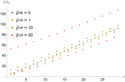
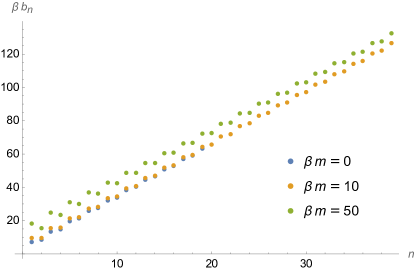
Figure 1: Lanczos coefficients for free massive scalar (left) and fermion (right) in $d=4$ dimensions. Values for the conformal (massless) cases we discussed in Dymarsky:2021bjq . For the scalar, introduction of $\tilde{m}=\beta m$ results in ‘‘persistent staggering’’ of $b_{n}$ around the conformal values (larger $\tilde{m}$ causes larger staggering amplitude) but does not change the slope $\pi n/\beta$. Lanczos coefficients split into two branches, see eq. 13. For fermions, asymptotically, $b_{n}$ grow linearly with the slope $\pi n/\beta$ and the $m$-dependent intercept. The main effect of mass is non-vanishing $a_{n}=\tilde{m}(-1)^{n}$.

Figure 2: Krylov complexity for the free massive scalar (left) and fermion (right) in $d=4$ dimensions. For the massless scalar $K=1+2\sinh^{2}(\pi t/\beta)$ is known analytically. The main effect of mass is the decrease of Krylov exponent $\lambda_{K}$.

4 CFTs on a sphere

In this section we consider a CFT places on a sphere and calculate Lanczos coefficients and Krylov complexity associated with the Wightman-ordered thermal two-point function. We consider two cases, 4d free massless scalar on ${\mathbb{S}}^{3}$ and holographic theories.

4.1 Free scalar on ${\mathbb{S}}^{3}\times{\mathbb{S}}^{1}$

We first consider a 4d free massless scalar compacted on a three-sphere. Because we are considering finite-temerature correlation function the 4d compactification manifold is ${\mathbb{S}}^{3}\times{\mathbb{S}}^{1}$. Corresponding thermal two-point function is given by, see Appendix C,

$$C(\tau,R) \propto \sum_{n,\ell\in{\mathbb{Z}}}{(\tau+1/2+n)^{2}-(R\ell)^{2}\over((\tau+1/2+n)^{2}+(R\ell)^{2})^{2}}=$$ (16)

$$\sum_{\ell\in{\mathbb{Z}}}{\pi^{2}\over 2}\left({1\over\cosh^{2}(\ell\pi R+i\pi\tau)}+{1\over\cosh^{2}(\ell\pi R-i\pi\tau)}\right)-{2\pi\over R}=\quad$$

$$\sum_{n\in{\mathbb{Z}}}{\pi^{2}\over R^{2}}{1\over\sinh^{2}((n+1/2+\tau)\pi/R)}.$$

Here $R$ is the radios of ${\mathbb{S}}^{3}$ measured in the units of $\beta$, which is the radius of ${\mathbb{S}}^{1}$. Euclidean time $\tau$ is defined as $\tau=it/\beta$. As expected the function is periodic in Euclidean time $\tau\rightarrow\tau+1$, but it is also periodic in Lorentzian time under $t\rightarrow 2\beta/R$, which follows e.g. from (16).

For any finite $R$, Lanczos coefficients split into even and odd branches, which grow linearly with $n$ but with different slopes, see Fig. 3. This can be seen analytically in the limit $R\rightarrow 0$ when $C(\tau)$ is exponentially small (unless $|\tau|=1/2$) and Lanczos coefficients, at leading order, are given by

$$b_{n}^{2}=\left({2\pi\over R}\right)^{2}\left\{\begin{array}[]{rc}(n+1)^{2}/4,&\,\,n=1,3,5,\dots\\ \frac{4n(n+1)^{2}}{n+2}e^{-\pi/R},&\,\,n=2,4,6,\dots\end{array}\right.$$ (19)

Numerically, this approximation is good already for $R\lesssim 1$.

In the opposite limit of large ${\mathbb{S}}^{3}$ the correlation function approaches that one of flat space, plus a correction $-2\pi/R$, plus the exponentially suppressed terms

$$C\propto{\pi^{2}\over\cos^{2}(\pi\tau)}-{2\pi\over R}+{\pi^{2}\over\cosh^{2}(\pi R-i\pi\tau)}+{\pi^{2}\over\cosh^{2}(\pi R+i\pi\tau)}+\dots$$ (20)

The exponentially suppressed terms are important for the asymptotic behavior of $b_{n}$. Neglecting them, i.e. keeping only first two terms in (20) yields the following expression for Lanczos coefficients, which we denote $b^{0}_{n}$,

$$(b_{n}^{0})^{2} = \pi^{2}n(n+1)-(-1)^{n}{c_{n}^{2}\over c_{n}R+d_{n}},\qquad n\geq 1,$$ (21)

$$c_{n} = \pi\left(2n+1-(-1)^{n}\right),\qquad d_{n}=4\left\lfloor\frac{n+1}{2}\right\rfloor\left(\psi^{(0)}\left(\frac{3}{2}\right)-\psi^{(0)}\left(\left\lfloor\frac{n+1}{2}\right\rfloor+\frac{1}{2}\right)-2\right).$$

Here $\psi^{0}$ is a polygamma function. This expression has incorrect asymptotic behavior for large $n$. Taking into account two more terms in (20) leads to

$$b_{n}^{2}=(b_{n}^{0})^{2}+8\pi^{2}(-1)^{n}n(n+1)(2n+1)e^{-2\pi R}+O(e^{-\pi R}/R),\qquad n\geq 1,$$ (22)

which still has incorrect the asymptotic. We thus conclude that to reproduce ‘‘two slopes’’ behavior

$$b_{n}=\left\{\begin{array}[]{c}\alpha_{1}(n+c_{1})+o(n),\qquad{\rm odd}\,n.\\ \alpha_{2}(n+c_{2})+o(n),\qquad{\rm even}\,n,\end{array}\right.\qquad n\gg 1.$$ (25)

would require taking into account an infinite serious of ever more exponentially suppressed terms into account. For all finite $R$, $\alpha_{1}>\alpha_{2}$; the opposite would contradict $C(t\rightarrow\infty)\rightarrow 0$. The ratio $\alpha_{1}/\alpha_{2}$ grows with $R^{-1}$, when radius is large two slopes are almost equal to each other and $\pi n/\beta$, but for small $R$ they are significantly different, with $\alpha_{2}$ quickly approaching zero.

Now we discuss Krylov complexity, which we calculate numerically. We find that $K(t)$ first increases, but then reaches its maximum and starts oscillating quasi-periodically, see the right panel of Fig. 3. This behavior is more pronounced for small $R$, while for large radius the behavior of $K(t)$ initially follows the flat space counterpart $K(t)=1+2\sinh^{2}(\pi t)$, before peaking at some finite value.

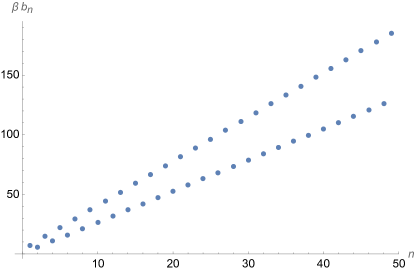
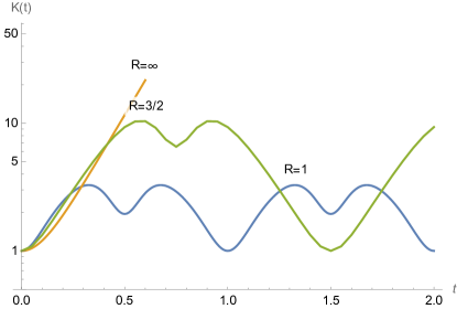
Figure 3: Left: Lanczos coefficients for free massless scalar compactified on ${\mathbb{S}}^{3}$ of radius $R=1$. Right: Krylov complexity $K(t)$ for radii $R=1$, flat space $K=1+2\sinh^{2}(\pi t)$, and $R=3/2$.

The two slopes behavior of $b_{n}$ is a novel phenomenon, not observed for physical systems previously. This goes beyond the universal operator growth hypothesis of Parker_2019 , which assumes a smooth asymptote of $b_{n}$. Similarly, capped Krylov complexity with the maximal value dependent on $R$ (the ratio of ${\mathbb{S}}^{3}$ and ${\mathbb{S}}^{1}$ radii) but not on the UV-cutoff is in tension with the proposal that qualitatively $K(t)$ is similar to holographic and computational complexities Barbon:2019wsy ; Rabinovici_2022 ; Rabinovici2022 . In the latter case, for a QFT on compact space, complexity would grow up to exponentially large values, controlled by the volume of ${\mathbb{S}}^{3}$ measured in the units of the UV cutoff. In case of $K(t)$ this growth was presumably supposed to come from the region of $b_{n}$ which is controlled by UV physics (and where $b_{n}$ are approximately constant while $K(t)$ grows linearly, see sections 5.2, 5.3 and Figs. 5 and 6). But the example above shows that the operator can be confined at the beginning of ‘‘Krylov chain,’’ in which case the values of $b_{n}$ for large $n$ do not matter.

Physically, it is tempting to relate two slopes behavior of $b_{n}$ and bounded $K(t)$ to finite volume of the space QFT is placed on, but we will see in the next section this is not true in full generality.

Mathematically, the two slopes behavior of $b_{n}$ is probably due to periodicity of $C(t)$ in Lorentzian time, or more broadly due to $f^{2}(\omega)$ being a sum of delta-functions for a not necessary periodic grid of values of $\omega$. We leave a proper investigation of this question for the future, together with the question of quantitatively relating $\alpha_{1},\alpha_{2}$ to some properties of $C(t)$. Here we only make one step in this direction and use the integral over Dyck paths developed in Avdoshkin_2020 to relate a particular combination of $\alpha_{1},\alpha_{2}$ to the location of pole of $C(t)$ in the complex plane, see Appendix E. Another question, which we also leave for the future, is to analytically relate maximal or time-averaged value of $K(t)$ to $\alpha_{i}$.

4.2 Holographic theories

Next we consider a holographic theory with the two-point function of heavy operators given by the sum over geodesic lengths in thermal AdS space, or black hole background, below and above the Hawking-Page transition correspondingly. In the former case the two-point function is

$$C(t)\propto\sum_{n}{1\over(\cosh((\tau+1/2+n)\beta)-1)^{\Delta}}$$ (26)

where the radius of boundary sphere is taken to be one. This expression is valid for all$\Delta$, not necessarily large, see e.g. Alday:2020eua . This expression is valid in all dimensions $d\geq 3$. We notice that, again, besides periodicity in Euclidean time $\tau\rightarrow\tau+1$, this function is periodic in Lorentzian time $t\rightarrow t+2\pi$. This is presumably the reason why $b_{n}$ behave qualitatively the same as in the previous subsection – they split into two branches for even and odd $n$, with both exhibiting asymptotic linear growth (25). The behavior of Krylov complexity also follows the pattern of free scalar on ${\mathbb{S}}^{3}$, it first grows but then oscillates quasi-periodically. We thus conclude that in holographic theories Krylov complexity can be UV-independent, thus making it qualitatively different from the holographic complexity Susskind:2014rva ; Brown:2015bva ; Brown:2015lvg ; Ben-Ami:2016qex ; Chapman:2016hwi ; Carmi:2017jqz ; Belin:2021bga .

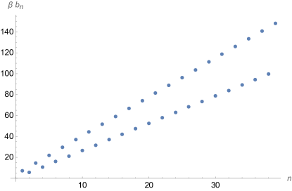
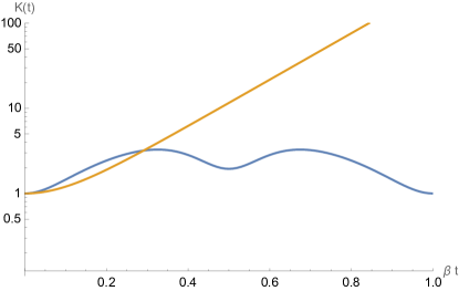
Figure 4: Left: Lanczos coefficients for thermal AdS background (26) with $\beta=2\pi$ and $\Delta=1$. Right: Krylov complexity for these parameters (blue) superimposed with $K(t)$ for flat space 2d CFT result $K=1+2\sinh^{2}(\pi t)$ (orange).

The discussion above applies to temperatures small enough, below the Hawking-Page transition. As the temperature increases the dual geometry is given by the BTZ background, assuming we focus specifically on the case of 2d theories. The two-point function in this background is given by Keski-Vakkuri:1998gmz ; Maldacena:2001kr

$$C(t)\propto\sum_{n}{1\over\left(\cos(2\pi\tau)+\cosh(4\pi^{2}n/\beta)\right)^{\Delta}}.$$ (27)

This function is, of course, periodic under $\tau\rightarrow\tau+1$, but there is no periodicity in Lorentzian time. As a result Lanczos coefficients have the ‘‘vanilla’’ behavior, growing linearly with the asymptote (9). In fact leading contribution comes from the $n=0$ term in (27), which is the same as the flat-space expression, with other terms for $\beta<2\pi$ giving very small corrections. Thus, numerically, $b_{n}^{2}$ are very close to $\pi^{2}(n+1)(n+2\Delta)/\beta^{2}$ Dymarsky:2021bjq . Accordingly, Krylov complexity grows exponentially with $\lambda_{K}=2\pi/\beta$.

The calculation in the BTZ background shows that two slopes behavior and capped $K(t)$ are not universal features of QFT on compact spaces, and the unbounded exponential growth of $K(t)$ is possible in the holographic settings. This prompts the question of how the inequality (1) fairs in different holographic scenarios. We see that above the Hawking-Page transition Krylov exponent $\lambda_{K}$ is well defined and equal to $2\pi/\beta$. This means second inequality in (1) is saturated and reduces to Maldacena-Shenker-Stanford bound, which is also saturated by holographic theories. Below the transition, Krylov complexity is bounded, hence $\lambda_{K}$ is not well-defined, or we can formally take it equal to zero. Exactly in the same scenario the OTOC correlator exhibits periodic recurrences, which also makes $\lambda_{\rm OTOC}$ ill-defined (or vanish) Anous:2019yku . In other words, (1) remains valid in both cases.

5 Temperature and UV-cutoff dependence of Lanczos
coefficients

We have seen in the previous sections that giving particles mass or placing a CFT on a compact background both have an explicit imprint on Lanczos coefficients and Krylov complexity. One feature, which nevertheless seems to be lost in the QFT case is the sensitivity of $b_{n}$ to chaos. Indeed, in all cases above $b_{n}$ exhibit linear growth (albeit sometimes by splitting into two branches), even though many considered theories are not chaotic. This mirrors the behavior we previously observed for CFTs in flat space Dymarsky:2021bjq and complements recent observation that non-chaotic systems with saddle-dominated scrambling also exhibit linear growth of $b_{n}$ Bhattacharjee_2022 .

This could be our final conclusion – that asymptotic of Lanczos coefficients is not a proper probe of chaos, but apparent success of this approach in case of discrete systems with finite local Hilbert space, in particular spin chains, hints this conclusion could be premature. As we mentioned above, for 1D lattice systems slowest possible decay of $f^{2}(\omega)$ is not exponential but super-exponential $f^{2}(\omega)\sim\omega^{-\omega}$ Avdoshkin_2020 . Yet for integrable spin chains $f^{2}(\omega)$ decays faster, as a Gaussian (which correspond to asymptotic growth $b_{n}\propto n^{1/2}$) or even becomes zero for $\omega$ exceeding certain size-independent threshold. This is is the case in all known examples, including preliminary numerical evidence for the XXZ model PhysRevE.100.062134 . On the contrary for the non-integrable 1d Ising model in traverse field it was recently proved in Cao_2021 that $f^{2}$ will decay with the slowest possible asymptotic, $f^{2}(\omega)\propto\omega^{-\omega}$. These results constitute non-trivial evidence for the ‘‘asymptotic of $b_{n}$ as a probe of chaos’’ stronger version of the universal operator growth hypothesis. We should mention, there is an additional evidence for the this hypothesis for D>1 lattice models: an analytic proof of $f^{2}\propto e^{-\omega/\omega_{0}}$ asymptotic for a non-integrable 2D lattice model bouch2015expected , and for the limit of SYK model Parker_2019 .

Apparent success with the spin chains and other discrete models and failure in field theoretic models suggest the issue could be related to the continuous nature of the latter. We elaborate on this in the next section.

5.1 Asymptotic of $f^{2}(\omega)$ and locality

While for the spin chains high frequency asymptotic of $f^{2}$ apparently contains some dynamical information, for continuous systems it is completely universal. Let’s consider the Fourier of the two-point correlation function in field theory. Then $f^{2}(\omega)$ has a simple interpretation as the sum of transition amplitudes between the one-particle states with energies $E_{i}$ and energies $E_{f}=E_{i}+\omega$. Its high-frequency asymptotic can be deduced from the following consideration. Let us consider a free quantum-mechanical particle propagating in 1D. Assuming the particle is fully localized, Heisenberg uncertainly principle implies the transition amplitude to a state with arbitrarily high energy is not suppressed (the Fourier of delta-function is a constant). After restoring $\beta$-dependent factors this means $f^{2}(\omega)$ will be proportional to $e^{-\beta\omega/2}$. Here locality of the initial state was crucial for the transition amplitude to states with large final energy to be unsuppressed. Going back to the two-point function $C(t)$, this translates into locality of the operator $A$. To see this in more detail, let us consider a same example, free quantum-mechanical particle with the Hamiltonian $H={p^{2}\over 2m}$, and an operator in the Heisenberg picture

$$A=e^{-x^{2}/a}.$$ (28)

We would like to evaluate (4) and find

$$f^{2}(\omega)=K_{0}(\beta(\beta+4am)\omega/2).$$ (29)

It’s clear that when $a$ is large, which corresponds to the de-localized wave-packet, the decay of $f^{2}$ is faster then the kenematicaly fixed value $f^{2}\propto e^{-\beta\omega/2}$ associated with the point-like operator $a\rightarrow 0$.

Provided the logic above is correct we may expect that in the case of a translationally-invariant lattice models similar behavior will emerge in the continuous (long wave) approximation, emerging in the low energy limit. We test this below in case of bosonic and fermionic lattice models. For the fixed value of coupling constants, effective wavelength is specified by inverse temperature $\beta$. Thus we expect that for large $\beta$ an approximate continuous description will emerge, leading to universal high frequency tail of $f$ and as well as universality of $b_{n}$ behavior. On the contrary, for small $\beta$ we expect to recover the diversity of $b_{n}$ behaviors previously observed in the literature, and in particular connection between the asymptotic of $b_{n}$ and chaos.

5.2 Integrable $XY$ model at finite temperature

The integrable periodic $XY$ spin chain

$$H=\sum_{i=1}^{N}(1+\gamma)S_{i}^{x}S_{i+1}^{x}+(1-\gamma)S_{i}^{y}S_{i+1}^{y}-h\,S_{i}^{z}$$ (30)

is solvable through the Jordan-Wigner transform and the two-point function at finite temperature

$$C(t)=\langle S^{z}(t)S^{z}(0)\rangle^{W}_{\beta}={\rm Tr}(e^{-\beta H/2}S^{z}(t)e^{-\beta H/2}S^{z})$$ (31)

is known explicitly, see Appendix D. We are interested in the thermodynamic limit of infinite $N$ and start with the case of isotropic XY model with $\gamma=h=0$, in which case

$$C(\tau)={1\over 4\pi^{2}}\left(\int_{-1}^{1}{dc\over\sqrt{1-c^{2}}}{\cosh(c\,\tau)\over\cosh(c\,\beta/2)}\right)^{2}.$$ (32)

Calculating $b_{n}$ numerically, for different values of $\beta$ reveals the following behavior. Initially Lanczos coefficients grow linearly as $b_{n}\approx\pi n/\beta$, and then saturate at some universal value $b_{n}\approx 1$, see Fig. 5. Clearly, initial region of linear growth increases for larger $\beta$. This has the following interpretation, at small temperatures the isotropic XY model becomes the free fermion CFT, hence Lanczos coefficients exhibit universal vanilla CFT behavior (9). For large $n$, when $b_{n}$ (which have dimension of energy) become of the order of UV-cutoff (which is of order one in our case), the universal QFT behavior is substituted by the true asymptotic behavior reflecting the dynamics of the lattice model. Since the isotropic XY model is free, Lanczos coefficients saturate at a fixed value, in full agreement with the previous observations that the asymptotic of $b_{n}$ is a probe of chaos (or lack thereof).

The main takeaway here is that to probe chaos, one should consider true asymptotic behavior of $b_{n}$ which is controlled by UV-cutoff physics. In the QFT models with an infinite cutoff, such as conformal field theories, the true asymptote is not accessible, giving way to the essentially universal vanilla behavior (of one or two linearly growing branches of $b_{n}$).

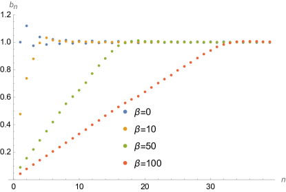
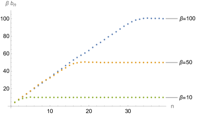
Figure 5: Both panels: Lanczos coefficients for the isotropic XY model (32).

5.3 Free bosons on the lattice

Next we consider free oscillators on the 1D lattice with periodic boundary conditions,

$$H={1\over 4}\sum_{i=1}^{N}\pi_{i}^{2}+(\phi_{i+1}-\phi_{i})^{2}+4\mu^{2}\phi_{i}^{2},$$ (33)

which becomes 1D free massive scalar theory in the continuous limit. We can think of this model as the 1+1 free scalar QFT with a cutoff. In the thermodynamic limit $N\rightarrow\infty$, when the mass $\mu$ and temperature $\beta^{-1}$ are chosen to be much smaller than the cutoff, $\beta\gg 1\gg\mu$, we expect the CFT in flat space behavior with $f^{2}\propto e^{-\beta\omega/2}$ and linearly growing Lanczos coefficients $b_{n}\sim\pi n/\beta$. At high energies we are dealing with the discrete integrable model of non-interacting particles with the energies belonging to a finite width zone. Accordingly $f^{2}(\omega)$ vanishes for $\omega$ exceeding certain value $\omega^{*}$. Thus, similarly to the isotropic XY model considered above, Lanczos coefficients are expected to approach a constant, signaling lack of chaos.

If $N$ is finite, in the long-wave limit the system is is described by free massive QFT placed on ${\mathbb{S}}^{1}$. In other words, the model (33) includes all three deformations we discuss in the paper: the mass, compact spatial manifold and the UV-cutoff. Accordingly, depending on the interplay between $\beta,\mu$ and $N$, at the level of $b_{n}$ we expect to see the combinations of some or all three features: persistent staggering, two-slopes behavior (since the theory is free, and the spectrum of excitations is equally-spaced), and field theory behavior below and saturation of $b_{n}$ near the UV-cutoff. An explicit calculation of (4) yields

$$C(\tau)\propto{1\over N}\sum_{{\rm k}=1}^{N}{1\over\epsilon_{k}}{\cosh(\epsilon_{k}\tau)\over\sinh(\epsilon_{k}\beta/2)},\qquad\epsilon_{k}=\sqrt{\sin^{2}(k)+\mu^{2}},\quad k={\pi{\rm k}/N}.$$ (34)

and the behavior of Lanczos coefficients for different $\beta$, $N$ and $\mu\ll 1$ is shown in Figure 6.

As expected, for essentially infinite $N$ and large $\beta$ initially $b_{n}$ grow linearly, as $b_{n}\approx\pi n/\beta$, but once the value of $b_{n}$ becomes the order of the cutoff (which is of order one in our case), they saturate to a constant. The punchline here is clear: for small temperatures the prolonged universal linear growth of $b_{n}$, dictated by the locality and Heisenberg uncertainty principle, will eventually give way to true asymptotic behavior governed by the discrete model emerging at the UV-cutoff scale. When $N$ is finite we observe the two slopes behavior, on top of the persistent staggering due to mass, and the transition toward true asymptote due to UV-cutoff.

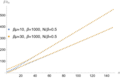
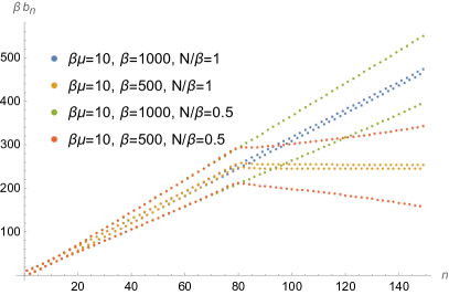
Figure 6: Lanczos coefficients for free bosons on the lattice (33) for different values of $\beta,\mu,N$ parameters. For large $\beta$ initial behavior of $b_{n}$ is that one in filed theory – coefficients grow linearly, either demonstrating persistent staggering and/or two-slopes behavior, see left panel. When $b_{n}$ approach UV-cutoff value the QFT behavior changes into one governed by the UV physics, see right panel.

6 Discussion

In the paper we calculated Lanczos coefficients $b_{n}$ and Krylov complexity $K(t)$ of local operators in several models of quantum field theory, free massive scalars and fermions, massless scalars compactified on a sphere, and a few holographic examples. Our calculations revealed that all three deformations of CFTs in flat space: giving particle mass, placing theory on a compact space, and introducing finite UV-cutoff has a clear imprint on $b_{n}$ and $K(t)$. Namely, mass leads to persistent staggering of $b_{n}$ (13) and decreases the Krylov exponent $\lambda_{K}$, while $K(t)$ still grows exponentially. Compact space, at least in certain cases, leads to two sloped behavior (25) and a capped Krylov complexity. Finite cutoff introduces a new asymptotic regime, where $b_{n}$ behavior is controlled by the lattice model at the UV scale.

These examples help us formulate several takeaway messages, clarifying the universal operator growth hypothesis of Parker_2019 and the role of Krylov complexity. First, asymptotic behavior of $b_{n}$ in physical systems goes beyond universality previously discussed in the literature, namely $b_{n}$ can split into two branches for even and odd $n$, each with its own asymptotic behavior. In particular this means that asymptotic behavior of $b_{n}$ is not mathematically equivalent or fully controlled by the high frequency asymptote of $f^{2}(\omega)$. Second, we clarified the role of temperature for $b_{n}$ in lattice models. Third, in field theory with an infinite UV-cutoff Lanczos coefficients do not probe chaotic behavior. But when a finite cutoff $\Lambda_{\rm UV}$ is introduced, by embedding the QFT into a lattice model, a true asymptotic regime of $b_{n}\gtrsim\Lambda_{\rm UV}$ emerges, which is conjecturally probing chaos in the underlying lattice model, modulo issues raised in Bhattacharjee_2022 . Here it is worth noting that a chaotic QFT can not emerge as a long wave limit from an integrable lattice model. Thus, with help of a finite UV-cutoff, universal operator growth hypothesis can be extended to quantum field theories.

Another takeaway message is the generalization of the Maldacena-Shenker-Stanford bound (1), which we tested in several non-trivial settings.

Finally, the examples of theories demonstrating two slopes behavior of $b_{n}$ and a capped $K(t)$ clearly show, Krylov complexity can have qualitatively different behavior than the holographic complexity Susskind:2014rva ; Brown:2015bva ; Brown:2015lvg ; Ben-Ami:2016qex ; Chapman:2016hwi ; Carmi:2017jqz ; Belin:2021bga .

Our work raise numerous questions, including a number of mathematical questions about the relation between $b_{n}$ and $C(t)$. Among them the features of $C(t)$ which lead to asymptotic persistent staggering (13) or two slopes (25) behavior and how to deduce $\alpha_{1},\alpha_{2},c_{1},c_{2}$ from $C(t)$. Here we presume a simple generalization of (9) is possible, though in section 4.1 we saw the example when the asymptotic of $b_{n}$ was dependent on the exponentially suppressed contributions to $C(t)$. There are many other questions, how to quantitatively relate $\lambda_{K}$ to $c_{1},c_{2}$ in case of persistent staggering and maximal or time-averaged $K(t)$ to $\alpha_{1},\alpha_{2}$ in case of two slopes behavior. There are also questions about physics of Krylov complexity. Can we prove generalized Maldacena-Shenker-Stanford bound (1) in full generality? Is there any holographic counterpart of $K(t)$? What is the behavior of $b_{n}$ and $K(t)$ in interacting QFTs? We leave these and other questions for the future.

Appendix A Massive free theories

A.1 Massive scalar

We start with a free massive scalar in ${\mathbb{R}}^{d}$ and calculate thermal two-point function

$$\langle\phi(\tau)\phi(-1/2)\rangle_{\beta}=\sum_{n=-\infty}^{\infty}{(-1)^{n}\over\beta}\int{d^{d-1}k\over(2\pi)^{d-1}}{e^{i2\pi n\tau}\over\big{(}{2\pi n\over\beta}\big{)}^{2}+k^{2}+m^{2}}.$$ (35)

Here $\tau=it/\beta$ is the Euclidean time. One operator is placed at $\tau=-1/2$, thus this is a Wightman-ordered correlator .

$$\langle\phi(\tau)\phi(-1/2)\rangle_{\beta}\propto{\rm Tr}(e^{-\beta H/2}\phi(t,x)e^{-\beta H/2}\phi(0,x)).$$

To evaluate (35) we substitute the sum over $n$ by a contour integral going over the singularities of $\sinh\big{(}{\tilde{k}_{0}\over 2}\big{)}$,

$$\langle\phi(\tau)\phi(-1/2)\rangle_{\beta}={\beta^{2-d}\over 4\pi i}\int_{\mathcal{C}}d\tilde{k}_{0}\int{d^{d-1}\tilde{k}\over(2\pi)^{d-1}}{e^{\tilde{k}_{0}\tau}\over\sinh\big{(}{\tilde{k}_{0}\over 2}\big{)}\big{(}\tilde{m}^{2}+\tilde{k}^{2}-\tilde{k}_{0}^{2}\big{)}}.$$ (36)

The contour can be deformed and closed through the infinite semicircle at ${\rm Re}\tilde{k}_{0}\rightarrow\infty$, yielding

$$C(t)={\rm Tr}(e^{-\beta H/2}\phi(t,x)e^{-\beta H/2}\phi(0,x))\propto{\beta^{2-d}\over(4\pi)^{d-1\over 2}\Gamma({d-1\over 2})}\int_{\tilde{m}}^{\infty}(y^{2}-\tilde{m}^{2})^{d-3\over 2}{\cosh(y\,\tau)\over\sinh(y/2)}dy.$$

A.2 Massive fermion

Similarly for the massive fermion

$$\langle\psi_{\alpha}^{\dagger}(\tau)\psi_{\sigma}(-1/2)\rangle_{\beta}={1\over\beta}\int{d^{d-1}k\over(2\pi)^{d-1}}\sum_{n=-\infty}^{\infty}{(-1)^{n}\over\beta}{\big{(}\pi(2n+1)\delta_{\alpha\sigma}+i\,\tilde{m}\,\gamma^{0}_{\alpha\sigma}\big{)}e^{i\pi(2n+1)\tau}\over\big{(}{(2n+1)\pi\over\beta}\big{)}^{2}+k^{2}+m^{2}}.$$ (37)

We work in Dirac representation such that $\gamma^{0}_{\alpha\sigma}=\pm\delta_{\alpha\sigma}$ and use the same trick with the contour integral

$$\langle\psi_{\alpha}^{\dagger}(\tau)\psi_{\sigma}(-1/2)\rangle_{\beta}={\beta^{1-d}\over 4\pi i}\int_{\mathcal{C}}d\tilde{k}_{0}\int{d^{d-1}\tilde{k}\over(2\pi)^{d-1}}{(\tilde{k}_{0}\pm\tilde{m})\,e^{\tilde{k}_{0}\tau}\over\cosh\big{(}{\tilde{k}_{0}\over 2}\big{)}\big{(}\tilde{k}^{2}+\tilde{m}^{2}-\tilde{k}_{0}^{2}\big{)}}.$$ (38)

After deforming the integration contour we arrive at

$${\rm Tr}(e^{-\beta H/2}\psi^{\dagger}(t,x)e^{-\beta H/2}\psi(0,x))\propto{\beta^{1-d}\over(4\pi)^{d-1\over 2}\Gamma\big{(}{d-1\over 2}\big{)}}\int_{|\tilde{m}|}^{\infty}dy\,(y^{2}-\tilde{m}^{2})^{d-3\over 2}{y\cosh(y\tau)\pm\tilde{m}\sinh(y\tau)\over\cosh\big{(}{y\over 2}\big{)}}.$$

Appendix B Lanczos coefficients for general $C(t)$

In the most general case, when $C(t)$ is not a real-valued even function, besides coefficients $b_{n}$, Lanczos coefficients also include $a_{n}$. Their definition in terms of Krylov basis can be found in e.g. dymarsky2020quantum , and the explicit expression in terms of $C(t)$ is as follows. For the analytically continued $C(\tau)$, $\tau=it$, we first define an $n\times n$ Hankel matrix of derivatives ${\mathcal{M}}^{(n)}_{ij}=C^{(i+j)}(\tau)$ and variables $\tau_{n}={\rm det}\,{\mathcal{M}}^{(n)}$, $\tau_{0}\equiv 1$. Then

$$\left.b_{n}={\tau_{n-1}\tau_{n+1}\over\tau_{n}^{2}}\right|_{\tau=0},$$ (39)

$$\left.a_{n}={d\over d\tau}(\tau_{n}-\tau_{n-1})\right|_{\tau=0}.$$ (40)

Appendix C Free scalar on ${\mathbb{S}}^{d-1}\times{\mathbb{S}}^{1}$

Let us consider a compact space $\mathbb{S}^{d-1}$ of radius $R$. The thermal correlation function of the scalar field living on $\mathbb{R}\times\mathbb{S}^{d-1}$ can be expressed in terms of the heat kernel $K_{\mathcal{M}}(t,x,y)=\langle x|\exp(-t\hat{D})|y\rangle$, see e.g., Vassilevich:2003xt

$$\langle\phi(x)\phi(y)\rangle_{\beta}=\int_{0}^{\infty}dtK(t,x,y)e^{-tm^{2}_{\text{eff}}}~{},$$ (41)

where $\mathcal{M}=\mathbb{S}^{1}\times\mathbb{S}^{d-1}$ ($\mathbb{S}^{1}$ represents a thermal circle parametrized by $\tau$), and $\hat{D}$ is the second order differential operator of the Laplace-Beltrami type,

$$\hat{D}=-{d\over d\tau^{2}}-\Delta_{\mathbb{S}^{d-1}}~{},$$ (42)

where $\Delta_{\mathbb{S}^{d-1}}$ is the scalar Laplacian on a sphere. Finally $m$ denotes the ’effective’ mass of the field under study

$$m^{2}_{\text{eff}}=m^{2}+\xi\mathcal{R}$$ (43)

where $\xi={d-2\over 4(d-1)}$ is the conformal coupling and $\mathcal{R}=\mathcal{R}(\mathbb{S}^{d-1})={(d-1)(d-2)/R^{2}}$ is the Ricci scalar of the background geometry.

The wave operators are separable on the product manifold $\mathbb{S}^{1}\times\mathbb{S}^{d-1}$ and hence the heat kernel can be expressed as the product of the two individual heat kernels on $\mathbb{S}^{1}$ and $\mathbb{S}^{d-1}$, i.e.,

$$K_{\mathcal{M}}=K_{\mathbb{S}^{1}}\,K_{\mathbb{S}^{d-1}}$$ (44)

$K_{\mathbb{S}^{1}}$ can be readily evaluated using the method of images. It is given by an infinite sum of the scalar heat kernels on $\mathbb{R}$, which are shifted by integer multiples of $\beta$ with respect to each other to maintain periodic boundary conditions for the scalar field on a circle, namely

$$K_{\mathbb{S}^{1}}(t,\tau)={1\over\sqrt{4\pi t}}\sum_{n=-\infty}^{\infty}e^{-{(\tau+n\beta)^{2}\over 4t}}$$ (45)

In fact, the heat kernel $K_{\mathbb{S}^{d-1}}$ is also known in full generality Camporesi:1994ga , e.g.,

$$K_{\mathbb{S}^{3}}(t,x,x)={e^{t/R^{2}}\over(4\pi t)^{3/2}}\sum_{n=-\infty}^{\infty}e^{-{\pi^{2}R^{2}n^{2}\over t}}\Big{(}1-2{\pi^{2}R^{2}n^{2}\over t}\Big{)}~{}.$$ (46)

In $d=4$, we thus get

$$C_{\phi}(\tau)=\sum_{n,\ell=-\infty}^{\infty}\int_{0}^{\infty}{dt\,e^{-t\,m^{2}}\over(4\pi t)^{2}}e^{-{(\tau+n\beta)^{2}+(2\pi R\ell)^{2}\over 4t}}\Big{(}1-2{\pi^{2}R^{2}\ell^{2}\over t}\Big{)}~{},$$ (47)

Integrating over $t$, yields

$$C_{\phi}(\tau) = m\sum_{n,\ell=-\infty}^{\infty}{A\,K_{1}(Am)-4B^{2}m\,K_{2}(Am)\over 4\pi^{2}A^{2}}~{}.$$

$$A^{2} = (\tau+n\beta)^{2}+(2\pi R\ell)^{2}\,,~{}B=\pi R\ell~{}.$$ (48)

For $\beta m,Rm\gg 1$ the sum is dominated by a few terms in the vicinity of $n=\ell=0$.

$C_{\phi}(\tau)$ simplifies in the case of conformally coupled scalar ($m=0$)

$$C_{\phi}(\tau)={1\over 4\pi^{2}}\sum_{n,\ell=-\infty}^{\infty}{(\tau+n\beta)^{2}-(2\pi R\ell)^{2}\over\big{(}(\tau+n\beta)^{2}+(2\pi R\ell)^{2}\big{)}^{2}}~{}.$$ (49)

Upon redefinition $\tau\rightarrow\beta\tau$ and $R\rightarrow\beta R$ we arrive at (16).

Appendix D Thermal 2pt function in XY model

Consider the Hamiltonian of integrable $XY$ model with periodic boundary conditions, $j=0$ is the same as $j=N$,

$$H=\sum_{j=1}^{N}\left[(1+\gamma)S^{x}_{j}S^{x}_{j+1}+(1-\gamma)S^{y}_{j}S^{y}_{j+1}\right]-h\sum_{j=1}^{N}S_{j}^{z}.$$ (50)

This chain is diagonalizable by the Jordan-Wigner transform NIEMEIJER1967377 , with the quasiparticle energies given by $\epsilon_{k}=\sqrt{(\cos k-h)^{2}+\gamma^{2}\sin^{2}k}$. Here $k$ varies between $0$ to $2\pi$. The autocorreation function at inverse temperature $\beta$ is defined as

$$C^{z}_{\beta}(t)\equiv\langle S^{z}_{0}S^{z}_{0}(t)\rangle_{\beta}={\rm Tr}(e^{-\beta H}S^{z}_{0}S^{z}_{0}(t))/{\rm Tr}(e^{-\beta H}).$$ (51)

Before giving the expression for $C^{z}_{\beta}(t)$ we first thermal expectation value

$$m_{z}(h)=\langle S^{z}_{0}\rangle_{\beta}=-\frac{1}{2\pi}\int_{0}^{\pi}dk\cos\left\{\tan^{-1}\left(\frac{\gamma\sin k}{\cos k-h}\right)\right\}\tanh\frac{\beta\epsilon_{k}}{2},$$ (52)

and one can show that $\lim\limits_{h\to 0}m^{z}(h)=0$. Finally, the autocorrelation function is given by

$$C^{z}_{\beta}(t)=m^{2}_{z}(h)+\left[\frac{1}{2\pi}\int\limits_{0}^{\pi}dk\left\{\cos(\epsilon_{k}t)+i\sin(\epsilon_{k}t)\tanh\frac{\beta\epsilon_{k}}{2}\right\}\right]^{2}$$ (53)

$$-\left[\frac{1}{2\pi}\int\limits_{0}^{\pi}dk\cos(2\lambda_{k})\left\{i\sin(\epsilon_{k}t)+\cos(\epsilon_{k}t)\tanh\frac{\beta\epsilon_{k}}{2}\right\}\right]^{2},$$

where $\lambda_{k}=\frac{1}{2}\tan^{-1}\frac{\gamma\sin k}{\cos k-h}$.

This expression becomes particularly simple, when we set $\gamma=0$, $h=0$ which corresponds to isotropic $XY$ model $H=\sum_{j=1}^{N}\left[S^{x}_{j}S^{x}_{j+1}+S^{y}_{j}S^{y}_{j+1}\right]$,

$$C_{\beta}(t)=\frac{1}{4\pi^{2}}\left(\int\limits_{-1}^{1}\frac{dc}{\sqrt{1-c^{2}}}\left[\cos(tc)-i\sin(tc)\tanh\frac{\beta c}{2}\right]\right)^{2},$$ (54)

which becomes even simpler upon the shift $t\to t-i\beta/2$ that gives the Whightman-ordered correlator, cf. with (32),

$$C_{\beta}^{W}(t)=\frac{1}{4\pi^{2}}\left[\int\limits_{-1}^{1}\frac{dc}{\sqrt{1-c^{2}}}\frac{\cos(tc)}{\cosh\beta c/2}\right]^{2}.$$ (55)

Appendix E Dyck paths integral for two slopes scenario

E.1 Integral over Dyck paths formalism for two branches

Here we will generalize the derivation of the asymptotic behavior of moments

$$\mu_{2n}=\int d\omega f^{2}(\omega)\omega^{2n}$$ (56)

from Avdoshkin_2020 to the case when $b_{n}$ form two continious bracnhes for large $n$, $b_{2n}=b_{even}(n)$ and $b_{2n+1}=b_{odd}(n)$. We start with the Dyck path sum representation of moments Parker_2019

$$\mu_{2n}=\sum_{\{h_{k}\}\in D_{n}}\prod_{k=0}^{2n-1}b_{(h_{k}+h_{k+1})/2},$$ (57)

where $D_{n}$ is the set of all Dyck paths.

We approximate each Dyck path with $h_{i}=1/2+2nf(i/2n)$, where $f(t)$ is a continious function defined on $0<t<1$ and satisfing $|f^{\prime}(t)|<1$. Let us consider N consequtive steps in a Dyck path, where $h_{k+1}-h_{k}=1$ for $n$ distinct values of $k$ so that $f^{\prime}=\frac{2n-N}{2}$. We additionally require that the index of $b$ is even $d$ times more than it is odd. We split the interval in pairs and we will denote the steps were value of $h$ increased (decreased) as "+" or "-" correspondingly.

For pairs "++" or "- -" one factor of $b$ has an odd index and another has an even one. For pairs "+-" and "-+" both factors will have the same parity that depends on the current value of $h_{i}$. If we denote the number of "++" pairs as $m$ and the number of opposite sign pairs that lead to two even factors as $l$ we obtain $d=4l-2n+4m$. Assuming our interval is small, its weight in (57) is given by

$$b_{odd}^{N/2-2l+n-2m}b_{even}^{N/2+2l-n+2m}=\sqrt{b_{odd}b_{even}}^{N}(b_{even}/b_{odd})^{2l-n+2m}.$$ (58)

The parameters satisfy $0<n<N$, $n-N/2<m<n/2$ and $0<l<n-2m$. The number of paths for fixed $n$, $m$ and $l$ is given by $C_{N/2}^{m}C_{N/2-m}^{n-2m}C_{n-2m}^{l}$. This product can be approximated with the help of the Stirling’s formula

$$\log C_{N/2}^{m}C_{N/2-m}^{n-2m}C_{n-2m}^{l}\approx$$

$$\frac{N}{2}\left[S(\alpha)+(1-\alpha)S\left(\frac{f^{\prime}+1-2\alpha}{1-\alpha}\right)+(f^{\prime}+1-2\alpha)S\left(\frac{\beta}{f^{\prime}+1-2\alpha}\right)\right],$$ (59)

where $n=N\frac{f^{\prime}+1}{2}$, $\alpha=\frac{m}{N/2}$, $\beta=\frac{l}{N/2}$ and

$$S(\alpha)=-\alpha\log\alpha-(1-\alpha)\log(1-\alpha).$$ (60)

We can evaluate the sum over $l$ and $m$

$$\sqrt{b_{odd}b_{even}}^{N}\sum_{m,l}C_{N/2}^{m}C_{N/2-m}^{n-2m}C_{n-2m}^{l}\epsilon^{2l-n+2m},$$ (61)

where $\epsilon=b_{even}/b_{odd}$ via the saddle point approximation. The function to be minimized is

$$W(\alpha,\beta,f^{\prime},\epsilon)=$$

$$S(\alpha)+(1-\alpha)S\left(\frac{f^{\prime}+1-2\alpha}{1-\alpha}\right)+(f^{\prime}+1-2\alpha)S\left(\frac{\beta}{f^{\prime}+1-2\alpha}\right)+(2\alpha+2\beta-f^{\prime}-1)\log\epsilon.$$

The saddle point equations are

$$\epsilon^{2}(1-2\alpha-\beta+f^{\prime})^{2}=\alpha(\alpha-f^{\prime}),$$ (62)

$$\epsilon^{2}(1-2\alpha-\beta+f^{\prime})=\beta.$$ (63)

It is solved by

$$\alpha^{*}=\frac{f^{\prime}(1-\epsilon^{2})^{2}-4\epsilon^{2}+(1+\epsilon^{2})\sqrt{4\epsilon^{2}+(\epsilon^{2}-1)^{2}f^{\prime 2}}}{2(\epsilon^{2}-1)^{2}},$$ (64)

$$\beta^{*}=\frac{\epsilon^{2}}{(\epsilon^{2}-1)^{2}}(1+\epsilon^{2}-\sqrt{4\epsilon^{2}+(\epsilon^{2}-1)^{2}f^{\prime 2}}).$$ (65)

Plugging this back in the expression for $W$, we obtain

$$W_{eff}(f^{\prime},\epsilon)=-\frac{f^{\prime}}{2}\log\frac{\epsilon^{2}f^{\prime 2}+f^{\prime}(f^{\prime}+\sqrt{4\epsilon^{2}+(\epsilon^{2}-1)^{2}f^{\prime 2}})+\epsilon^{2}(2+f^{\prime}\sqrt{4\epsilon^{2}+(\epsilon^{2}-1)f^{\prime 2}})}{2\epsilon^{2}(1-f^{\prime})^{2}}+$$

$$+\log\frac{(\epsilon^{2}-1)^{2}}{\epsilon+\epsilon^{3}-\epsilon\sqrt{4\epsilon^{2}+(\epsilon^{2}-1)^{2}(f^{\prime})^{2}}}.$$

Finally, this gives us a path integral representation of moments (56)

$$\mu_{2n}=\int\mathcal{D}f(t)e^{n\int\limits_{0}^{1}dt\left(W(f^{\prime},\epsilon)+2\log b(f)\right)}.$$ (66)

We can verify that this path integral reduces to the path integral for a single branch developed in Avdoshkin_2020 when we set $\epsilon=1$ ($b_{even}=b_{odd}$). While the second term is singular as $\epsilon\to 0$ it is finite if we carefully take the limit

$$\lim\limits_{\epsilon\to 1}W_{\text{eff}}(f^{\prime},\epsilon)=2S\left(\frac{f^{\prime}+1}{2}\right).$$ (67)

Alternatively, the saddle point configuration simplifies to

$$\alpha^{*}=\frac{(1+f^{\prime})^{2}}{4},~{}~{}\beta^{*}=\frac{(1-f^{\prime})^{2}}{4}.$$ (68)

and again we obtain $W(\alpha^{*},\beta^{*},f^{\prime},1)=2s\left(\frac{f^{\prime}+1}{2}\right)$. This agrees with the expected result, since $W$ is multiplied by $n$ (it used to be $2n$ in the single branch case).

E.2 Evaluation of the path integral for two slopes

Here we assume that $\epsilon=\text{const}$ and $\sqrt{b_{odd}(n)b_{even}(n)}=\alpha n$. The action in this case reads

$$I=\int\limits_{0}^{1}dt\left(W(f^{\prime},\epsilon)+2\log f\right),$$ (69)

where have neglected the constant term $2\log(2\alpha n)$ in the integral since it does not affect the shape of the saddle point. Varying $I$ with respect to $f(t)$, we obtain the EOMs

$$-\frac{2}{f(t)}=\frac{f^{\prime\prime}}{1-(f^{\prime})^{2}}\frac{(1+\epsilon^{2}+\sqrt{4\epsilon^{2}+(-1+\epsilon^{2})^{2}(f^{\prime})^{2}})}{\sqrt{4\epsilon^{2}+(-1+\epsilon^{2})^{2}(f^{\prime})^{2}}}.$$ (70)

We can lower the order of equation by defining $g(f)=f^{\prime}$:

$$\frac{(1+\epsilon^{2}+\sqrt{4\epsilon^{2}+(1-\epsilon^{2})^{2}g^{2}})g^{\prime}g}{(1-g^{2})\sqrt{4\epsilon^{2}+(1-\epsilon^{2})^{2}g^{2}}}=-\frac{2}{f}.$$ (71)

And the solution is

$$g^{2}=\frac{\epsilon^{4}+(1-(c_{1}f)^{2})^{2}-2\epsilon^{2}(1+(c_{1}f)^{2})}{(1-\epsilon^{2})^{2}},$$ (72)

where $c_{1}$ is some constant. By requiring $g(f(1/2)=f_{0})=0$, we arrive at

$$c_{1}f_{0}=1-\epsilon,~{}c_{1}=\frac{1-\epsilon}{f_{0}}.$$ (73)

Having found $g$ as a function of $f$, we can now solve for $f$ as a function of $t$. Setting $g=f^{\prime}$ leads to

$$\frac{1}{c_{1}}H(c_{1}f,\epsilon)=\frac{t}{1-\epsilon^{2}}+c_{2},$$ (74)

where

$$H(x,\epsilon)=\frac{(1+\epsilon)\sqrt{1-\left(\frac{x}{1-\epsilon}\right)^{2}}\sqrt{1-\left(\frac{x}{1+\epsilon}\right)^{2}}F\left(\arcsin(\frac{x}{1+\epsilon}),\left(\frac{1+\epsilon}{1-\epsilon}\right)^{2}\right)}{\sqrt{\epsilon^{4}+(1-x^{2})^{2}-2\epsilon^{2}(1+x^{2})}},$$ (75)

and $F(x,a)$ is the incomplete elliptic integral (we use the same conventions as Wolfram Mathematica). Taking the limit $x\to 1-\epsilon$ we have

$$H(1-\epsilon,\epsilon)=\frac{K\left[\left(\frac{1-\epsilon}{1+\epsilon}\right)^{2}\right]}{1+\epsilon},$$ (76)

where $K$ is the complete elliptic integral.

We can use this expression to find $c_{1}$ and the value of the function at the maximum ($t=1/2$)

$$2(1-\epsilon)K\left[\left(\frac{1-\epsilon}{1+\epsilon}\right)^{2}\right]=c_{1},~{}f_{0}=\frac{1}{2K\left[\left(\frac{1-\epsilon}{1+\epsilon}\right)^{2}\right]}.$$ (77)

As a consistency check we verify that for $\epsilon=1$ we reproduce the old result $\lim\limits_{\epsilon\to 1}f_{0}=1/\pi$ (the solution for a sinlge branch was $\frac{\sin(\pi t)}{\pi}$).

The ‘‘on-shell’’ action can be rewritten as

$$I(\epsilon)=2\int\limits_{0}^{f_{0}}\frac{df}{g(f)}\left(W(g(f),\epsilon)+2\log f\right),$$ (78)

where $f_{0}$ and $g(f)$ are given by

$$f_{0} = \frac{1}{2K\left[\left(\frac{1-\epsilon}{1+\epsilon}\right)^{2}\right]},$$ (79)

$$g^{2}(f) = \frac{(f^{2}-f^{2}_{0})}{(1+\epsilon)^{2}f_{0}^{4}}\left[(1-\epsilon)^{2}f^{2}-(1+\epsilon)^{2}f_{0}^{2}\right].$$ (80)

Written explicitly, this integral is rather cumbersome and difficult to deal with. The numeric plot of $I$ as a function of $\epsilon$ is shown in Fig. 7.

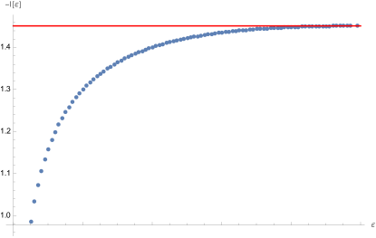
Figure 7: Numeric values of $-I(\epsilon)$ are shown in blue, the red line is $-\log\frac{2}{\pi e}$, the value of the action known analytically for a single branch, that corresponds to $-I(1)$.

The asymptotic behavior of the moments is

$$\boxed{\log\mu_{2n}\approx nI(\epsilon)+2n\log(2\alpha n).}$$ (81)

If $\epsilon=1$, $I(1)=2\log\frac{2}{\pi e}$ and $\log\mu_{2n}\approx 2n\log\frac{4\alpha n}{\pi e}$.

E.3 Small $\epsilon$ expansion

In this subsection, we will determine the small $\epsilon$ behavior of $I(\epsilon)$. First of all, since we know the exact value of $f(1/2)$ we can find the limit

$$f(1/2)=f_{0}\approx\frac{1}{|\log\epsilon|}.$$ (82)

Next, at small $\epsilon$ (72) simplifies to

$$f^{\prime}(t)=1-(f(t)/f_{0})^{2},$$ (83)

which is solved by $f(t)=f_{0}\tanh(t/f_{0})$. While this solution seems to not be symmetric under $t\to 1-t$, it should be thought of as only applicable at $t<1/2$ and defined by symmetry for $t>1/2$. This function is essentially constant for $t\gg\frac{1}{|\log\epsilon|}$ and, thus, stitching it with a different function at $t=1/2$ is appropriate.

Now, we expand $W(f^{\prime},\epsilon)$.

$$W(f^{\prime},\epsilon)\approx S(f^{\prime})+|\log\epsilon|(1-f^{\prime}),$$ (84)

$$I(\epsilon)=2\int\limits_{0}^{1/2}dt(S(f^{\prime})-|\log\epsilon|f^{\prime})+|\log\epsilon|+4\int\limits_{0}^{1/2}dt\log(f),$$ (85)

$$\int\limits_{0}^{\infty}(S(f^{\prime})-|\log\epsilon|f^{\prime})\approx\frac{\pi^{2}/4-\log(4)}{|\log\epsilon|}-1,$$ (86)

$$\int\limits_{0}^{1/2}dt\log(f)\approx-\frac{\pi^{2}}{8}\frac{1}{|\log\epsilon|}-\frac{1}{2}\log|\log\epsilon|.$$ (87)

Collecting all the terms together,

$$I(\epsilon)=|\log\epsilon|-2\log|\log\epsilon|-2-\frac{2\log 4}{|\log\epsilon|}+\cdots.$$ (88)

Thus, the leading behavior is

$$\log\mu_{2n}\approx n|\log\epsilon|-2n\log|\log\epsilon|+2n\log(2\alpha n).$$ (89)

E.4 $1-\epsilon$ expansion

Let us define $\epsilon=1-\delta$. We can expand

$$f_{0}\approx\frac{1}{\pi}-\frac{\delta^{2}}{16\pi}.$$ (90)

The correction to the action is

$$\delta S=\frac{\delta^{2}}{4}\int\limits_{0}^{1}dt(1-(f^{\prime})^{2}).$$ (91)

Since the variation of the action vanishes on the saddle point solution the contribution coming from the change in the saddle point will be of order $\delta^{4}$. Thus, to leading order we only need to evaluate the value of (91),

$$\delta S=\frac{\delta^{2}}{8}.$$ (92)

Finally,

$$\log\mu_{2n}=2n\left(\log\frac{4\alpha n}{\pi e}+\frac{\delta^{2}}{16}\right)+O(\delta^{4}).$$ (93)

References

- (1) D. E. Parker, X. Cao, A. Avdoshkin, T. Scaffidi and E. Altman, A universal operator growth hypothesis, Physical Review X 9 (2019) .
- (2) T. A. Elsayed, B. Hess and B. V. Fine, Signatures of chaos in time series generated by many-spin systems at high temperatures, Physical Review E 90 (2014) 022910.
- (3) A. Avdoshkin and A. Dymarsky, Euclidean operator growth and quantum chaos, Physical Review Research 2 (2020) .
- (4) A. Dymarsky and M. Smolkin, Krylov complexity in conformal field theory, Phys. Rev. D 104 (2021) L081702 [2104.09514].
- (5) B. Bhattacharjee, X. Cao, P. Nandy and T. Pathak, Krylov complexity in saddle-dominated scrambling, Journal of High Energy Physics 2022 (2022) .
- (6) J. Maldacena, S. H. Shenker and D. Stanford, A bound on chaos, Journal of High Energy Physics 2016 (2016) 106.
- (7) Y. Gu, A. Kitaev and P. Zhang, A two-way approach to out-of-time-order correlators, Journal of High Energy Physics 2022 (2022) .
- (8) L. Susskind, Computational Complexity and Black Hole Horizons, Fortsch. Phys. 64 (2016) 24 [1403.5695].
- (9) A. R. Brown, D. A. Roberts, L. Susskind, B. Swingle and Y. Zhao, Holographic Complexity Equals Bulk Action?, Phys. Rev. Lett. 116 (2016) 191301 [1509.07876].
- (10) A. R. Brown, D. A. Roberts, L. Susskind, B. Swingle and Y. Zhao, Complexity, action, and black holes, Phys. Rev. D 93 (2016) 086006 [1512.04993].
- (11) O. Ben-Ami and D. Carmi, On Volumes of Subregions in Holography and Complexity, JHEP 11 (2016) 129 [1609.02514].
- (12) S. Chapman, H. Marrochio and R. C. Myers, Complexity of Formation in Holography, JHEP 01 (2017) 062 [1610.08063].
- (13) D. Carmi, S. Chapman, H. Marrochio, R. C. Myers and S. Sugishita, On the Time Dependence of Holographic Complexity, JHEP 11 (2017) 188 [1709.10184].
- (14) A. Belin, R. C. Myers, S.-M. Ruan, G. Sárosi and A. J. Speranza, Does Complexity Equal Anything?, Phys. Rev. Lett. 128 (2022) 081602 [2111.02429].
- (15) S.-K. Jian, B. Swingle and Z.-Y. Xian, Complexity growth of operators in the SYK model and in JT gravity, Journal of High Energy Physics 2021 (2021) .
- (16) V. Balasubramanian, P. Caputa, J. Magan and Q. Wu, Quantum chaos and the complexity of spread of states, 2022. 10.48550/ARXIV.2202.06957.
- (17) A. Dymarsky and A. Gorsky, Quantum chaos as delocalization in krylov space, Physical Review B 102 (2020) 085137.
- (18) D. J. Yates, A. G. Abanov and A. Mitra, Lifetime of almost strong edge-mode operators in one-dimensional, interacting, symmetry protected topological phases, Phys. Rev. Lett. 124 (2020) 206803.
- (19) D. J. Yates, A. G. Abanov and A. Mitra, Dynamics of almost strong edge modes in spin chains away from integrability, Physical Review B 102 (2020) .
- (20) D. J. Yates, A. G. Abanov and A. Mitra, Long-lived period-doubled edge modes of interacting and disorder-free Floquet spin chains, 2105.13766.
- (21) D. J. Yates and A. Mitra, Strong and almost strong modes of Floquet spin chains in Krylov subspaces, Phys. Rev. B 104 (2021) 195121 [2105.13246].
- (22) J. D. Noh, Operator growth in the transverse-field ising spin chain with integrability-breaking longitudinal field, Physical Review E 104 (2021) .
- (23) F. B. Trigueros and C.-J. Lin, Krylov complexity of many-body localization: Operator localization in Krylov basis, 2112.04722.
- (24) C. Liu, H. Tang and H. Zhai, Krylov complexity in open quantum systems, 2022. 10.48550/ARXIV.2207.13603.
- (25) Z.-Y. Fan, Universal relation for operator complexity, Physical Review A 105 (2022) .
- (26) A. Kar, L. Lamprou, M. Rozali and J. Sully, Random matrix theory for complexity growth and black hole interiors, Journal of High Energy Physics 2022 (2022) .
- (27) J. L. F. Barbón, E. Rabinovici, R. Shir and R. Sinha, On The Evolution Of Operator Complexity Beyond Scrambling, JHEP 10 (2019) 264 [1907.05393].
- (28) E. Rabinovici, A. Sánchez-Garrido, R. Shir and J. Sonner, Operator complexity: a journey to the edge of krylov space, Journal of High Energy Physics 2021 (2021) .
- (29) E. Rabinovici, A. Sánchez-Garrido, R. Shir and J. Sonner, Krylov localization and suppression of complexity, Journal of High Energy Physics 2022 (2022) .
- (30) E. Rabinovici, A. Sánchez-Garrido, R. Shir and J. Sonner, Krylov complexity from integrability to chaos, Journal of High Energy Physics 2022 (2022) .
- (31) P. Caputa, J. M. Magan and D. Patramanis, Geometry of krylov complexity, 2021. 10.48550/ARXIV.2109.03824.
- (32) P. Caputa and S. Datta, Operator growth in 2d CFT, Journal of High Energy Physics 2021 (2021) .
- (33) P. Caputa and S. Liu, Quantum complexity and topological phases of matter, 2022. 10.48550/ARXIV.2205.05688.
- (34) R. Heveling, J. Wang and J. Gemmer, Numerically probing the universal operator growth hypothesis, Phys. Rev. E 106 (2022) 014152.
- (35) K. Adhikari and S. Choudhury, osmological rylov omplexity, 2022. 10.48550/ARXIV.2203.14330.
- (36) K. Adhikari, S. Choudhury and A. Roy, rylov omplexity in uantum ield heory, 2022. 10.48550/ARXIV.2204.02250.
- (37) W. Mück and Y. Yang, Krylov complexity and orthogonal polynomials, 2022. 10.48550/ARXIV.2205.12815.
- (38) A. Bhattacharya, P. Nandy, P. P. Nath and H. Sahu, Operator growth and krylov construction in dissipative open quantum systems, 2022. 10.48550/ARXIV.2207.05347.
- (39) N. Hörnedal, N. Carabba, A. S. Matsoukas-Roubeas and A. del Campo, Ultimate speed limits to the growth of operator complexity, Communications Physics 5 (2022) .
- (40) S. Guo, Operator growth in su(2) yang-mills theory, 2022. 10.48550/ARXIV.2208.13362.
- (41) M. Afrasiar, J. K. Basak, B. Dey, K. Pal and K. Pal, Time evolution of spread complexity in quenched lipkin-meshkov-glick model, 2022. 10.48550/ARXIV.2208.10520.
- (42) V. Balasubramanian, J. M. Magan and Q. Wu, A tale of two hungarians: Tridiagonalizing random matrices, 2022. 10.48550/ARXIV.2208.08452.
- (43) S. Baek, Krylov complexity in inverted harmonic oscillator, 2022. 10.48550/ARXIV.2210.06815.
- (44) B. Bhattacharjee, X. Cao, P. Nandy and T. Pathak, An operator growth hypothesis for open quantum systems, 2212.06180.
- (45) M. Alishahiha and S. Banerjee, A universal approach to Krylov State and Operator complexities, 2212.10583.
- (46) H. Araki, Gibbs states of a one dimensional quantum lattice, Communications in Mathematical Physics 14 (1969) 120.
- (47) V. Viswanath and G. Müller, The Recursion Method: Application to Many-Body Dynamics, vol. 23. Springer Science & Business Media, 2008.
- (48) L. F. Alday, M. Kologlu and A. Zhiboedov, Holographic correlators at finite temperature, JHEP 06 (2021) 082 [2009.10062].
- (49) E. Keski-Vakkuri, Bulk and boundary dynamics in BTZ black holes, Phys. Rev. D 59 (1999) 104001 [hep-th/9808037].
- (50) J. M. Maldacena, Eternal black holes in anti-de Sitter, JHEP 04 (2003) 021 [hep-th/0106112].
- (51) T. Anous and J. Sonner, Phases of scrambling in eigenstates, SciPost Phys. 7 (2019) 003 [1903.03143].
- (52) T. LeBlond, K. Mallayya, L. Vidmar and M. Rigol, Entanglement and matrix elements of observables in interacting integrable systems, Phys. Rev. E 100 (2019) 062134.
- (53) X. Cao, A statistical mechanism for operator growth, Journal of Physics A: Mathematical and Theoretical 54 (2021) 144001.
- (54) G. Bouch, The expected perimeter in eden and related growth processes, Journal of Mathematical Physics 56 (2015) 123302.
- (55) D. V. Vassilevich, Heat kernel expansion: User’s manual, Phys. Rept. 388 (2003) 279 [hep-th/0306138].
- (56) R. Camporesi and A. Higuchi, Spectral functions and zeta functions in hyperbolic spaces, J. Math. Phys. 35 (1994) 4217.
- (57) T. Niemeijer, Some exact calculations on a chain of spins 12, Physica 36 (1967) 377.