Restricting to the chip architecture maintains the quantum neural network accuracy,
if the parameterization is a $2$-design

Abstract

In the era of noisy intermediate scale quantum devices, variational quantum circuits (VQCs) are currently one of the main strategies for building quantum machine learning models. These models are made up of a quantum part and a classical part. The quantum part is given by a parametrization $U$, which, in general, is obtained from the product of different quantum gates. By its turn, the classical part corresponds to an optimizer that updates the parameters of $U$ in order to minimize a cost function $C$. However, despite the many applications of VQCs, there are still questions to be answered, such as for example: What is the best sequence of gates to be used? How to optimize their parameters? Which cost function to use? How the architecture of the quantum chips influences the final results? In this article, we focus on answering the last question. We will show that, in general, the cost function will tend to a typical average value the closer the parameterization used is from a $2$-design. Therefore, the closer this parameterization is to a $2$-design, the less the result of the quantum neural network model will depend on its parametrization. As a consequence, we can use the own architecture of the quantum chips to defined the VQC parametrization, avoiding the use of additional swap gates and thus diminishing the VQC depth and the associated errors.

I Introduction

Quantum machine learning is an emerging interdisciplinary area of study that involves quantum computing and machine learning biamonte ; schuld . This investigation path seeks to create a quantum machine learning model with greater computational power than its classical counterparts. For this, phenomena that are only possible to obtain in the quantum domain are used, such as entanglement and superposition. Currently, in the era of noisy intermediate-scale quantum devices, variational quantum circuits have proved to be one of the best strategies for building quantum machine learning models. Variational quantum circuits cerezo ; tilly are built using a quantum part and a classical part. The quantum part is obtained from a parameterization $U(\theta)$ composed of different quantum gates and with parameters $\theta$. In turn, the classical part refers to an optimizer whose objective is to minimize a cost function $C$. For this, the classical optmizer iteractively updates the parameters $\theta$ of the parameterization $U$.

Although the number of works in this area has grown in recent years, there are still many questions and problems to be resolved. One example of such a problem is the disappearance of the gradient, which is also known as barren plateaus BR_cost_Dependent ; BR_Entanglement_devised_barren_plateau_mitigation ; BR_Entanglement_induced_barren_plateaus ; BR_expressibility ; BR_noise ; BR_gradientFree . This problem is related to the fact that as the number of parameters in the parameterization $U$ increases, the gradient of the cost function tends to zero. This makes the optimization of the parameters impossible. Some methods to mitigate this problem have already been suggested friedrich ; BR_initialization_strategy ; BR_Large_gradients_via_correlation ; BR_LSTM ; BR_layer_by_layer . Furthermore, problems such as parameters optimization Friedrich_nes ; Rebentrost ; Schuld_Evaluating , influence of the expressiveness of the parameterization Expressibility_Sim ; Hubregtsen , and influence of the architecture of the quantum chips nash ; bravyi still have to be addressed.

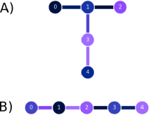
Figure 1: Illustration of IBM’s A) Lima and B) Manila chips architectures.

In this article, we study how the quantum computer chip architecture influences the efficiency of a quantum neural network model. For example, IBM quantum processors have different chip architectures. This architecture determines which qubits pairs interact directly. For example, for the Lima chip, Fig. 1 A, qubits 1 and 3 interact directly, i.e., we can implement a controlled NOT (CNOT) gate through their direct interaction. However, on the Manila chip, Fig. 1 B, we cannot apply the CNOT gate directly between the qubits 1 and 3. To do this, we must initially apply a SWAP gate, for example, between qubits 2 and 3 and only then apply the CNOT between qubits 1 and 3. As a consequence of this, the depth of the parameterization $U$ will increase, leading to serious problems due to noise on chips with multiple qubits, for which it would be necessary to use multiple SWAP gates. For escaping from this kind of problem, it would be tempting to consider parametrizations $U$ involving CNOT gates applied only to pairs of qubits that are directly connect in the quantum chip. But this raises the question about how this will affect the efficiency of the corresponding VQC. It is this question that we will investigate in this article.

The remainder of this article is organized as follows. In Sec. II, we describe the three main stages of a quantum neural netwok, i.e., the data encoding, parametrization and measurement stages. In Sec. III, we prove our main results regarding the typical non-influence of different paramentrizations on the VQC efficiency. In Sec. IV, we give details about our simulation method. With this, In Sec. V, we present the results obtained in our simulations. Finally, In. Sec. VI, we give our final remarks.

II Quantum neural networks

Quantum neural networks are models of neural networks inspired by classical models. These models can be divided into two main parts. The first part, the quantum one, is built using initially a parametrization $V$ whose task is to map our classical data into a quantum state. Some data encoding examples are the wave function encoder

$$|\boldsymbol{x}\rangle:=\frac{1}{\|\boldsymbol{x}\|_{2}^{2}}\sum_{i=1}^{2^{N}}x_{i}|i\rangle,$$ (1)

the dense angle encoding

$$|\boldsymbol{x}\rangle=\bigotimes_{i=1}^{N/2}\big{(}\cos(\pi x_{2i-1})|0\rangle+e^{2\pi ix_{2i}}\sin(\pi x_{2i-1})|1\rangle\big{)},$$ (2)

and the qubit encoding

$$|\boldsymbol{x}\rangle=\bigotimes_{i=1}^{N}\big{(}\cos(x_{i})|0\rangle+\sin(x_{i})|1\rangle\big{)}.$$ (3)

After encoding the input data into quantum states, we apply a parametrization $U(\boldsymbol{\theta})$. This parametrization is generally obtained from the composition of different quantum gates, such as CNOT, SWAP, rotation gates, etc. In a quantum neural network model, this part is the analogue of the hidden layers used in a classical neural network model. In general, we can write the parametrization as follows

$$U(\boldsymbol{\theta})=\prod_{l=1}^{L}U_{l}W_{l},$$ (4)

where $L$ is the parametrization depth, $U_{l}$ is an arbitrary parametrization and $W_{l}$ is a parameterization that does not depend on the parameters. For example, this parametrization can be obtained from the product of applied CNOT gates in the qubits. For the purposes of this article, we define the parametrization such that

$$U_{l}=\otimes_{j=1}^{N}R_{\sigma}(\theta_{l,j}),$$ (5)

where $R_{\sigma}(\theta_{l,j})=e^{-i\theta_{l,j}\sigma/2}$ with $\sigma\in\{\sigma_{x},\sigma_{y},\sigma_{z}\}$ being one of the Pauli matrices.

Finally, the third part that makes up the quantum circuit is the measurement. There are different ways of defining these measurements, and their choice has great relevance to the problem. For example, in Ref. BR_cost_Dependent it was shown that the phenomenon of barren plateaus is related to the choice of these measurements. However, in general, we can define the measurement as

$$f(x,U)=Tr[U\rho U^{\dagger}H],$$ (6)

where $\rho:=|\boldsymbol{x}\rangle\langle\boldsymbol{x}|$ and $H$ is an observable. For instance, we can use $H:=|i\rangle\langle i|$, where $|i\rangle$ is one of the computational base states. Or we can utilize $H:=\otimes_{i=1}^{N}\sigma_{i}$, with $\sigma_{i}$ being one of the Pauli matrices applied to the qubit indexed $i$ and $N$ is the number of qubits used.

The second part of a quantum neural network consists of a classical optimizer that, using a cost function $C$, updates the parameters of the parameterization $U$. Different proposals have already been made Friedrich_nes ; Rebentrost ; Schuld_Evaluating , however, as in classical neural networks, in general this optimization is done using the gradient of $C$.

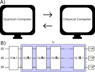
Figure 2: A) Illustration of the operation of a variational quantum circuit. These models work in a hybrid way, that is, using a quantum computer and a classical computer. In the quantum computer the quantum circuit will be run and in the classical computer the classical optimizer will be run. B) Illustration of a quantum circuit with three qubits.

III Effect of the variational quantum circuit parametrization

Our main objective here to answer the question: Does the architecture of the quantum chips influence the efficiency of a quantum machine learning model? As we discussed in the previous section, the parametrization in general can be written in the form given by Eq. (4), with each $U_{l}$ given by Eq. (5). Initially, we observe that the parametrization $U_{l}$ given by Eq. (5) does not depend on the architecture of the chip that will be used, since each one of its quantum gates acts on a single qubit. However, the parameterization $W_{l}$, obtained when using gates that do not depend on the parameters, as for example the CNOT, SWAP, CZ, CY gates, will depend on the architecture of the quantum chip.

If we look at the two architectures in Fig. 1, we will see that the qubits are arranged in different ways. If, for example, we want to apply a CNOT gate on qubits 2 and 3, we have two possible situations. If the two qubits are next to each other, as is case B in Fig. 1, we can apply the CNOT gate directly. However, for the case A in Fig. 1, where the qubits are not side by side, we cannot apply the interaction-based quantum gate directly. In situations alike to this last case, we must exchange the states of the qubits so that both are side by side. This is done by applying a SWAP gate between the qubits that must be exchanged. In the case if Fig. 1 B, we must initially apply a SWAP gate between qubits 1 and 2. Only after that we can apply the CNOT between qubits 2 and 3. After that, we must again apply a SWAP gate between qubits 1 and 2. As a consequence of this need for using SWAP gates, that are composed by three CNOT gates, in order to be able to apply interaction-base quantum gates that act on more than one qubit for qubits that are not directly connected, the parametrization depth, and consequently the noise, tends to increase. So, in the NISQ era, characterized among other factors by the presence of noise, this increase in circuit depth has serious unwanted implications.

Thus, one is led naturally to ask if for quantum machine learning models it is in fact necessary to make use of these nonparametrized quantum gates involving qubits that do not interact directly. For classical machine learning models, one observes that, in general, what determines the success of the model is the training data that will be used and the number of parameters of the neural network, but not the architecture itself. Thus, we can conjecture that quantum models will also be more dependent on data than on the architecture. As a consequence, we can choose not to use gates that act on more than one qubit for qubits that are not directly connected. In order to prove this conjecture, we start by defining the cost function as

$$C=\frac{1}{D}\sum_{i=1}^{D}(f(x_{i},U)-y_{i})^{2},$$ (7)

where $D$ is the size of our training dataset, $f(x_{i},U)$ is the quantum model output defined in Eq. (6) with the parametrization $U$ given by Eq. (4) and $y_{i}$ is the desired output given the input $x_{i}$. With this we can state the following theorem.

Theorem 1

Let the cost function be defined in Eq. (7), let the training dataset be $\mathcal{D}:=\{x_{i},y_{i}\}_{i=1}^{D}$, and let the parametrization be given by Eq. (4). We have that the average value of the cost function over the parametrizations $U$ will be limited by

$$\mathbb{E}_{U}[C]\geqslant\frac{1}{D}\sum_{i=1}^{D}Var_{U}[f(x_{i},U)].$$ (8)

To prove this theorem, we start by rewriting the cost function in Eq. (7) as

$$C=\frac{1}{D}\sum_{i=1}^{D}(f(x_{i},U)-\mu+\mu-y_{i})^{2},$$ (9)

where $\mu:=\mathbb{E}_{U}[f(x_{i},U)]$. So we have

$$\begin{split}\mathbb{E}_{U}[C]=&\frac{1}{D}\sum_{i=1}^{D}\mathbb{E}_{U}[(f(x_{i},U)-\mu+\mu-y_{i})^{2}]\\ =&\frac{1}{D}\sum_{i=1}^{D}\mathbb{E}_{U}[(f(x_{i},U)-\mu)^{2}+\\ &+2(f(x_{i},U)-\mu)(\mu-y_{i})+(\mu-y_{i})^{2}].\end{split}$$ (10)

Since $\mathbb{E}_{U}[2(f(x_{i},U)-\mu)(\mu-y_{i})]=0$, then Eq. (10) reduces to

$$\mathbb{E}_{U}[C] =\frac{1}{D}\sum_{i=1}^{D}\mathbb{E}_{U}[(f(x_{i},U)-\mu)^{2}+(\mu-y_{i})^{2}]$$

$$=\frac{1}{D}\sum_{i=1}^{D}\mathbb{E}_{U}[(f(x_{i},U)-\mu)^{2}]+\mathbb{E}_{U}[(\mu-y_{i})^{2}]$$

$$\geqslant\frac{1}{D}\sum_{i=1}^{D}Var_{U}[f(x_{i},U)].$$ (11)

With this we complete the proof of Theorem 1. From this Theorem, it follows the following corollary.

Corollary 1

Let the cost function be defined by Eq. (7), let the training dataset be $\mathcal{D}:=\{x_{i},y_{i}\}_{i=1}^{D}$, and let the parametrization to be given by the Eq. (4). Then the deviation of the cost function is bounded as follows:

$$|C-\mathbb{E}_{U}[C]|\leqslant\frac{d+1}{d^{2}(d^{2}-1)}\bigg{(}|Tr[H]^{2}|+d|Tr[H^{2}]|\bigg{)}+|C|,$$ (12)

with $d=2^{N}$, where $N$ is the number of qubits used in the VQC.

To prove this Corollary, we must first calculate the variance of Eq. (6), which is defined as $Var_{U}[f(x_{i},U)]=\mathbb{E}_{U}\big{[}(f(x_{i},U))^{2}\big{]}-\big{(}\mathbb{E}_{U}[f(x_{i},U)]\big{)}^{2}$. If $U$ is $1$-design, then we have BR_cost_Dependent

$$\mathbb{E}_{U}[f(x_{i},U)]=\int d\mu(U)Tr[U\rho_{i}U^{\dagger}H]=\frac{Tr[H]}{d}.$$ (13)

Above we use $Tr[\rho_{i}]=1\ \forall i$. If $U$ is a $2$-design, then it follows that BR_cost_Dependent

$$\mathbb{E}_{U}\big{[}(f(x_{i},U))^{2}\big{]} =\int d\mu(U)Tr[U\rho_{i}U^{\dagger}H]Tr[U\rho_{i}U^{\dagger}H]$$

$$=\frac{Tr[H]^{2}+Tr[H^{2}]}{d^{2}-1}\bigg{(}1-\frac{1}{d}\bigg{)},$$ (14)

where we used $Tr[\rho_{i}^{2}]=1$, since $\rho_{i}$ are pure states. So, using Eqs. (13) and (14) we get

$$Var_{U}[f(x_{i},U)]=\frac{1-d}{d^{2}(d^{2}-1)}Tr[H]^{2}+\frac{d-1}{d(d^{2}-1)}Tr[H^{2}].$$ (15)

From Theorem 1 and from the triangle inequality for complex numbers, we obtain

$$\big{|}C-\mathbb{E}_{U}[C]\big{|} \leq\Big{|}C-\frac{1}{D}\sum_{i=1}^{D}Var_{U}[f(x_{i},U)]\Big{|}$$ (16)

$$\leqslant|C|+\Big{|}\frac{1}{D}\sum_{i=1}^{D}Var_{U}[f(x_{i},U)]\Big{|}$$ (17)

$$\leqslant|C|+\frac{1}{D}\sum_{i=1}^{D}\big{|}Var_{U}[f(x_{i},U)]\big{|}.$$ (18)

Now, using the variance obtained in Eq. (15), we get

$$|C-\mathbb{E}_{U}[C]|\leqslant\frac{d-1}{d^{2}(d^{2}-1)}\bigg{(}\big{|}Tr[H]^{2}\big{|}+d\big{|}Tr[H^{2}]\big{|}\bigg{)}+|C|.$$ (19)

With this, we complete the proof of the corollary.

As a consequence of Corollary 1, we see that the deviation of the cost function $C$ approaches its mean value $\mathbb{E}_{U}[C]$ as the number of qubits increases. This behavior will also be impacted by the choice of observable. Therefore, with this we can conclude that, for large parametrizations, we can simply disregard the application of gates that act on more than one qubit, if they do not interact directly in a quantum chip.

IV Simulation method

To exemplify the behavior predicted in the previous section, two sets of experiments were carried out. In the first set of experiments, the parametrization $U$, given by Eq. (4), was generated randomly. For this first set of experiments, $300$ different parametrizations were generated. For each of these parametrizations, $20$ training epochs were used. The optimizer used was Adam, with a learning rate of $0.001$. The number of qubits used was varied from $2$ to $10$. The parametrization depth was also varied, where we used $L=2$, $L=4$, and $L=6$. We utilized two observables $H$. The first being defined as $H=\mathbb{I}\otimes\sigma_{Z}$, where the $\sigma_{Z}$ Pauli matrix was always applied to the last qubit of the quantum circuit. We also used the observable $H=\mathbb{I}\otimes|0\rangle\langle 0|$, measuring $|0\rangle\langle 0|$ also on the last qubit.

It should be noted that, to obtain the random parametrizations, we applied the definition given by Eq. (4) with each $U_{l}$ given by Eq. (5). During each experiment, the $R_{\sigma}$ gates that appear in Eq. (5) were randomly generated. Moreover, the $W_{l}$ parametrization was also randomly generated, where all qubits could be correlated, i.e. we could use, for example, the CNOT gate between all the qubit pairs. Besides the CNOT gate, the CZ and CY gates could also be used, in addition to identity, in which case the qubits would not interact.

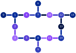
Figure 3: Illustration of IBM’s Guadalupe chip.

For the second set of experiments, fixed parametrizations were applied. That is to say, $U$ was previously defined. Initially, the simulations were performed without any restrictions. However, in the second step, restrictions were used in the parametrization $U$. The restriction used was that the gates that act on more than one qubit could only be applied to qubits that were directly connected in the quantum chip. To know which qubits would be side by side, IBM’s Guadalupe quantum chip was used as a model; see Fig. 3. For these experiments, both the number of qubits and the parametrization depth were varied, where the values used were equal to those used in the first set of experiments. Besides, the same optimizer with the same learning rate as in the previous experiments were used here.

In the first set of experiments, $300$ different parametrizations were generated. We used a high number of parametrizations in order to have greater precision in the results obtained. However, in the second set of experiments, as the parametrization is fixed with the only difference being the initial parameters, we chose to do each experiment 50 times.

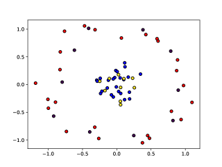
Figure 4: Example of item of the dataset used when training quantum neural network models. The red and blue dots are the training data. The yellow and purple dots are the test data.

Finally, the data used for training the models were obtained using the machine learning library scikit-learn Scikit_learn_ref . In Fig. 4, an example of training data used during these experiments is illustrated. In Fig. 5 is illustrated how the encoding of data in a quantum state was done for all experiments. As the input data is composed of vectors of two elements, we choose to encode the two values in all qubits.

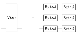
Figure 5: Illustration of the way data was encoded in a quantum state. In this example only three qubits are shown. However, the same encoding was used in all the experiments, independent of the number of qubits involved.

Fig. 6 shows how the parametrization is done for the set of experiments where it is not fixed by the chip architecture. We choose this parametrization because it is one of the most affected by the chip architecture, since all qubits are correlated through the CNOT gate.

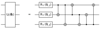
Figure 6: Illustration of the $U_{l}$ parametrization for the case where it is not fixed by the chip architecture.

V Simulation results

In this section, we present the results obtained in the numerical simulations. We start by presenting the results obtained by randomly generating the parametrization $U$. From the results presented in Fig. 7, we see that as the parametrization depth and number of qubits increase, the cost function tends typically towards its average value. According to the Corollary 1, this behavior should not depend on the parametrization depth. We argue that this happens due to the fact that the result obtained in the Corollary 1 is actually an approximation, since we used the assumption that the generated parametrizations were $2$-designs. So, as we have no way of guaranteeing that the generated parametrization is in fact a $2$-design, we can expect behaviors that deviate from the theoretical prediction. Thus, we can also assume that as the parametrization depth increases, the more the VQC will approach to a $2$-design, so that their behavior will be more similar to the theoretical behavior.

We should also observe that, according to the Corollary 1, the deviation of the cost function $C$ from its mean value is also determined by the value of the cost function itself. Therefore, if the value of the cost function is very large, this deviation will be too. However, the smaller the value of the cost function, the smaller is this deviation. What we can observe is that for all experiments, as the model was being trained, that is, the cost function was decreasing, we can see that the concentration of the cost function was close to the average value, confirming what the Corollary 1 predicts.

In the second set of simulations, Figs. 8 and 9, we use a fixed parameterization. Again, we use the observables $H=\mathbb{I}\otimes\sigma_{Z}$ and $H=\mathbb{I}\otimes|0\rangle\langle 0|$. In the first graph, Fig. 8, we see how the quantum neural network behaves when we use $H=\mathbb{I}\otimes\sigma_{Z}$ as an observable . In Fig. 8 A, the behavior of the quantum neural network is shown when the parameterization is fixed and we do not use any restriction, that is, we use the parameterization shown in Fig. 6 without any restriction. In Fig. 8 B, we see how it behaves when we use the chip’s architecture as a restriction, in this case the restriction was that the CNOT gates, which appear in Fig.6, could only be used between qubits that were side by side. side by side, for this we use the Guadalupe chip, Fig. 3.

In the second graph, Fig. 9, we see again how the quantum neural network behaves, however, in this case we use $H=\mathbb{I}\otimes|0\rangle\langle 0|$ as the observable. As in the previous case, in figure Fig.9 A, the behavior of the quantum neural network is shown when the parameterization is fixed and we do not use any restrictions. In figure Fig.9 B, we see how it behaves when we use the chip architecture as a restriction. Again, in this case the restriction was that the CNOT gates, which appear in Fig. 6, could only be applied between qubits that are directly connected in the chip. For that, we used the Guadalupe chip as a reference, see Fig. 3.

We argue again that for both cases, Fig. 8 and 9, as the parameterization depth increases, the more the VQC will approach a 2-design, so its behavior will be more similar to the theoretical behavior.

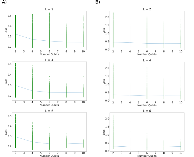
Figure 7: Behavior of a quantum neural network model as the number of qubits increases for different depths of the parametrization. The green dots show how $300$ different parametrizations behave after training. For training the parametrizations, $20$ epochs were used. The blue line shows the average value for the $300$ parametrizations. A) The observable used here was $H=\mathbb{I}\otimes|0\rangle\langle 0|$ . B) The observable used here was $H=\mathbb{I}\otimes\sigma_{Z}$.

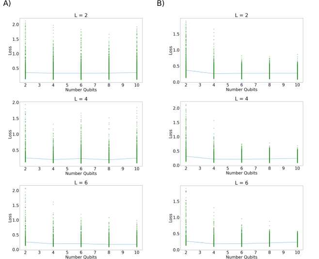
Figure 8: Behavior of a quantum neural network model as the number of qubits increases for different depths of the parametrization. In this numerical simulations, we using parametrization show in Fig. 6. For training the parametrization, $20$ epochs were used. For the two figures, we used the observable $H=\mathbb{I}\otimes\sigma_{Z}$. A) It shows how the quantum neural network behaves when no constraints are applied. B) It shows how the quantum neural network behaves when we use the constraints of the chip architecture shown in Fig. 3.

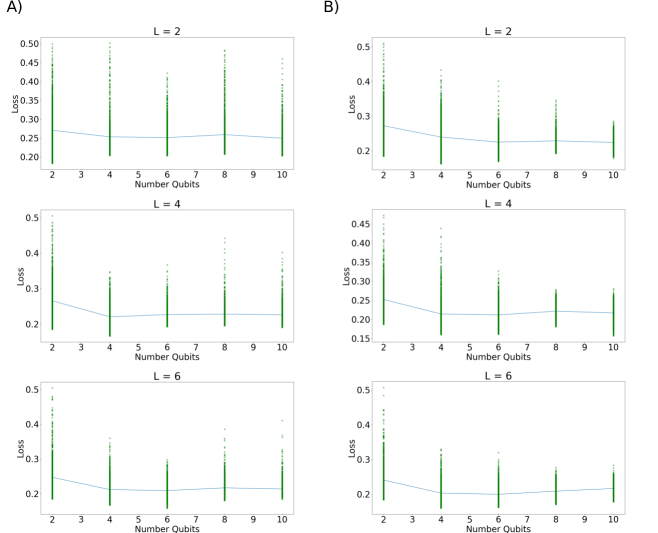
Figure 9: Behavior of a quantum neural network model as the number of qubits increases for different depths of the parametrization. In this numerical simulations, we used the parametrization shown in Fig. 6. For training the parametrization, $20$ epochs were used. For the two figures, we used the observable $H=\mathbb{I}\otimes|0\rangle\langle 0|$. A) It shows how the quantum neural network behaves when no constraints are applied. B) It shows how the quantum neural network behaves when we use the constraints of the chip architecture shown in Fig. 3.

VI Conclusions

In this work we aimed to answer the question: does the architecture of quantum chips influence the results of a quantum machine learning model? Just like classical machine learning models, where the results quality are more related to the data used than to the architecture of the model, for quantum models we showed that the results quality is more related to the size of the parameterization, that is to say, to how many qubits are used, and to the depth of the parameterization, choice of the observable, and the cost function $C$ itself. Therefore, the result does not really depend on the parameterization $U$. Therefore we can disregard quantum gates that act on more than one qubit if they are not directly connected in a quantum chip. Furthermore, the numerical results obtained confirm this conclusion, where we saw that in fact the cost function tends to an average value as the parameterization increases regardless of the parameterization used $U$. However, we must emphasize that this behavior will depend on how much the parameterization used approaches to a $2$-design, where the closer it is from a $2$-design, the closer its behavior will be to our theoretical prediction.

References

- (1) J. Biamonte et al., Quantum machine learning, Nature 549, 195 (2017).
- (2) M. Schuld and F. Petruccione, Machine Learning with Quantum Computers (Springer Nature Switzerland, 2021).
- (3) M. Cerezo et al., Variational Quantum Algorithms, Nat. Rev. Phys. 3, 625 (2021).
- (4) J. Tilly et al., The Variational Quantum Eigensolver: A review of methods and best practices, Phys. Rep. 986, 1 (2022).
- (5) M. Cerezo, A. Sone, T. Volkoff, L. Cincio, and P.J. Coles, Cost Function Dependent Barren Plateaus in Shallow Parametrized Quantum Circuits, Nat. Commun. 12, 1791 (2021).
- (6) T. L. Patti, K. Najafi, X. Gao, and S. F. Yelin, Entanglement devised barren plateau mitigation, Phys. Rev. Research 3, 033090 (2021).
- (7) C. O. Marrero, M. Kieferová, and N. Wiebe, Entanglement-induced barren plateaus, PRX Quantum 2, 040316 (2021).
- (8) Z. Holmes, K. Sharma, M. Cerezo, and P. J. Coles, Connecting ansatz expressibility to gradient magnitudes and barren plateaus, PRX Quantum 3, 010313 (2022).
- (9) S. Wang et al., Noise-induced barren plateaus in variational quantum algorithms, Nature Communications 12, 6961 (2021).
- (10) A. Arrasmith, M. Cerezo, P. Czarnik, L. Cincio, and P. J. Coles, Effect of barren plateaus on gradient-free optimization, Quantum 5, 558 (2021).
- (11) L. Friedrich and J. Maziero, Avoiding barren plateaus with classical deep neural networks, Phys. Rev. A 106, 042433 (2022).
- (12) E. Grant, L. Wossnig, M. Ostaszewski, and M. Benedetti, An initialization strategy for addressing barren plateaus in parametrized quantum circuits, Quantum 3, 214 (2019).
- (13) T. Volkoff and P. J. Coles, Large gradients via correlation in random parameterized quantum circuits, Quantum Science and Technology 6, 025008 (2021).
- (14) G. Verdon et al, Learning to learn with quantum neural networks via classical neural networks, https://doi.org/10.48550/arXiv.1907.05415 (2019).
- (15) A. Skolik, J. R. McClean, M. Mohseni, P. van der Smagt, and M. Leib, Layerwise learning for quantum neural networks, Quantum Machine Intelligence 3, 5 (2021).
- (16) L. Friedrich and J. Maziero, Natural evolutionary strategies applied to quantum-classical hybrid neural networks, http://arxiv.org/abs/2205.08059 (2022).
- (17) P. Rebentrost et al., Quantum gradient descent and Newton’s method for constrained polynomial optimization, New Journal of Physics 21, 073023 (2019).
- (18) M. Schuld et al., Evaluating analytic gradients on quantum hardware, Phys. Rev. A 99, 032331 (2019).
- (19) S. Sim, P. D. Johnson, and A. Aspuru-Guzik, Expressibility and entangling capability of parameterized quantum circuits for hybrid quantum-classical algorithms, Advanced Quantum Technologies 2, 1900070 (2019).
- (20) T. Hubregtsen et al., Evaluation of parameterized quantum circuits: On the relation between classification accuracy, expressibility, and entangling capability, Quantum Machine Intelligence 3, 1 (2021).
- (21) B. Nash, V. Gheorghiu, and M. Mosca, Quantum circuit optimizations for NISQ architectures, Quantum Sci. Technol. 5, 025010 (2020).
- (22) S. Bravyi, O. Dial, J.M. Gambetta, D. Gil, and Z. Nazario, The future of quantum computing with superconducting qubits, Journal of Applied Physics 132, 160902 (2022).
- (23) F. Pedregosa et al., Scikit-learn: Machine learning in Python, The Journal of machine Learning research 12, 2825 (2011).