A posteriori error analysis and adaptivity for a VEM discretization of the Navier-Stokes equations

Abstract

We consider the Virtual Element method (VEM) introduced by Beirão da Veiga, Lovadina and Vacca in 2016 for the numerical solution of the steady, incompressible Navier-Stokes equations; the method has arbitrary order $k\geq 2$ and guarantees divergence-free velocities. For such discretization, we develop a residual-based a posteriori error estimator, which is a combination of standard terms in VEM analysis (residual terms, data oscillation, and VEM stabilization), plus some other terms originated by the VEM discretization of the nonlinear convective term. We show that a linear combination of the velocity and pressure errors is upper-bounded by a multiple of the estimator (reliability). We also establish some efficiency results, involving lower bounds of the error. Some numerical tests illustrate the performance of the estimator and of its components while refining the mesh uniformly, yielding the expected decay rate. At last, we apply an adaptive mesh refinement strategy to the computation of the low-Reynolds flow around a square cylinder inside a channel.

Keywords A posteriori estimator, Adaptivity, Virtual element method, Navier-Stokes equations, Computational fluid dynamics

1 Introduction

Since their inception (Beirão da Veiga et al. (2013, 2014)), Virtual Element Methods (VEM) have experienced an explosive growth of interest in the community devoted to the numerical solution of partial differential equations. VEM can be viewed as a generalization of Finite Element Methods, in which domain partitions formed by elements with rather arbitrary shapes are allowed; polytopal meshes are the prime example. The success of VEM is certainly due to the fact that they permit a high geometric flexibility (which, e.g., facilitates mesh generation, or local adaptive mesh refinements) without giving up the benefits of FEM, such as the use of weak formulations, or the use of polynomials in the calculation of elemental matrices.

Among the various applications of Virtual Element Methods, we highlight here the numerical solution of fluid-dynamics problems, such as the equations describing an incompressible flow. We refer to the papers Beirão da Veiga et al. (2017, 2018) which initiated this research line, followed by other contributions such as, e.g., Wang et al. (2020, 2021). A remarkable advantage of VEM over FEM is the easiness in generating discretizations which produce divergence-free velocities, thereby satisfying the continuity equation exactly. Another interesting feature is the possibility of handling meshes with cut elements, as those encountered, e.g., in problems of fluid-structure interactions; see Beirão da Veiga et al. (2021a) for an example. Furthermore, adaptive mesh refinement – a natural procedure in the presence of localized structures such as vortices – gains efficiency from using virtual elements, for which the hanging nodes generated by local refinement are simply viewed as edge separators, and need not be removed. We refer to Beirão da Veiga et al. (2021b) for an interesting realization of this new perspective.

The present paper is a contribution to the development of adaptive Virtual Element Methods for the stationary incompressible Navier-Stokes equations in dimension 2. More precisely, we devise a residual-based a posteriori error estimator for the VEM discretization of order $k\geq 2$ introduced in Beirão da Veiga et al. (2018), we prove reliability and efficiency results, and we use the estimator in designing an adaptive refinement algorithm, which we apply to a classical fluid-dynamic problem in Wind Engineering, the flow around a square cylinder (Breuer et al. (2000)).

Concerning the a posteriori error analysis for VEM, after the pioneering work Cangiani et al. (2017) for a general second-order elliptic problem, we mention the a posteriori estimator given in Wang et al. (2020) for the Stokes equations, and the one in Wang et al. (2021) for the Navier-Stokes equations. Note however that the VEM discretization considered hereafter differs from the one in Wang et al. (2021), and we base our robustness analysis of the estimator on a general framework due to Ainsworth and Oden (1997).

Our adaptive algorithm is based on the classical loop $\texttt{SOLVE}\to\texttt{ESTIMATE}\to\texttt{MARK}\to\texttt{REFINE}$, with SOLVE realized by the VEM discretization Beirão da Veiga et al. (2018) of order $k=2$, and MARK realized by Dörfler’s criterion. In the application, following Breuer et al. (2000), we consider a 2D rectangular channel with a square obstacle symmetrically placed astride the horizontal axis, and we use meshes made of geometrically square elements, obtained by quad-tree refinements. These elements are indeed virtual elements: a hanging nodes created by a refinement splits the edge of a square into two aligned edges, thereby generating a polygon with 5 or more edges.

The paper is organized as follows. Section 2 introduces the steady continuous Navier-Stokes problem, while Section 3 describes the VEM discretization adopted following Beirão da Veiga et al. (2018). Our main results related to the a posteriori error analysis is contained in Section 4, in particular here we prove an upper bound of the error in terms of the estimator, together with some lower bounds. In Section 5, we first validate our estimator with some numerical tests; then, we introduce the adaptive algorithm and we apply it to the flow around a square obstacle at Reynolds number $<60$ (for which the solution is steady), showing the sequence of adaptive meshes and producing an accurate estimate of the length of the recirculation zone past the obstacle. The conclusions follow in Section 6.

Notation. We denote by $\|\cdot\|_{0,A}$ the $L^{2}(A)$-norm of a function (which may be a scalar, a vector, or a tensor) defined on a Lipschitz domain $A$ (in one or two dimensions), and by $(\cdot\,,\cdot)_{A}$ the inner product in $L^{2}(A)$. Similarly, we denote by $|\cdot|_{k,A}=|\cdot|_{H^{k}(A)}$ and $\|\cdot\|_{k,A}=\|\cdot\|_{H^{k}(A)}$ the Sobolev semi-norm and norm of order $k$ in $A$. Furthermore, the notation $P\lesssim Q$ means $P\leq C\,Q$, where $C>0$ is a constant independent of the considered discretization and the Reynolds number.

2 The continuous problem

We consider the steady Navier-Stokes problem in a polygonal domain $\Omega\subset\mathbb{R}^{2}$ under mixed Dirichlet-Neumann boundary conditions:

$$\text{\em find}\quad(\mathbf{u},p)\quad\text{\em such that}\quad\begin{cases}-\nu\mathbf{\Delta}\mathbf{u}+(\mathbf{\nabla}\mathbf{u})\mathbf{u}-\nabla p=\mathbf{f}\quad\text{in $\Omega$}\,,\\ \nabla\cdot\mathbf{u}=0\quad\text{in}\quad\Omega\,,\\ \mathbf{u}=\mathbf{g}\quad\text{on}\quad\Gamma_{D}\subseteq\partial\Omega\,,\\ (\nu\mathbf{\nabla}\mathbf{u}+p\mathbf{I})\mathbf{n}=\mathbf{t}\quad\text{on}\quad\Gamma_{N}=\partial\Omega\setminus\Gamma_{F}\,,\\ \end{cases}$$ (1)

where $\mathbf{u}$ and $p$ are the velocity and pressure solutions, $\mathbf{f}$ is the external force, and $\mathbf{g}$ and $\mathbf{t}$, resp., are the Dirichlet and Neumann data, resp. (with $\int_{\partial\Omega}\mathbf{g}\cdot\mathbf{n}=0$ if $\Gamma_{D}=\partial\Omega$). All physical quantities as dimensionless, with respect to a characteristic velocity $U$ and a characteristic length $L$. The quantity $1/\nu>0$ is the Reynolds number $Re$. The pressure sign is chosen as in Beirão da Veiga et al. (2018). Note that $(\mathbf{\nabla}\mathbf{u})\mathbf{u}=(\mathbf{u}\cdot\mathbf{\nabla})\mathbf{u}$, where the tensor $\mathbf{\nabla}\mathbf{u}$ is the Jacobian matrix of $\mathbf{u}$.

We will develop our theoretical analysis under the simplifying assumption of homogeneous Dirichlet conditions on the whole of $\partial\Omega$ (whereas numerical results will be given in the general case). Therefore, we introduce the spaces

$$\mathbf{V}:=[H^{1}_{0}(\Omega)]^{2}\,,\qquad Q:=L^{2}_{0}(\Omega)=\big{\{}q\in L^{2}(\Omega)\quad\text{s.t.}\quad\int_{\Omega}q\,\text{d}\Omega=0\big{\}}\,,$$

with norms $\|\mathbf{v}\|_{\mathbf{V}}=\|\mathbf{v}\|_{1,\Omega}$ and $\|q\|_{Q}=\|q\|_{0,\Omega}$, respectively, and we formulate the problem variationally as follows: find $(\mathbf{u},p)\in\mathbf{V}\times Q$ such that

$$\begin{cases}a(\mathbf{u},\mathbf{v})+c(\mathbf{u};\mathbf{u},\mathbf{v})+b(\mathbf{v},p)=(\mathbf{f},\mathbf{v})\quad\forall\,\mathbf{v}\in\mathbf{V}\,,\\ b(\mathbf{u},q)=0\quad\forall\,q\in Q\,,\end{cases}$$ (2)

with

$$\begin{split}&a(\mathbf{u},\mathbf{v}):=\int_{\Omega}\nu\,\mathbf{\nabla}\mathbf{u}:\mathbf{\nabla}\mathbf{v}\,\text{d}\Omega,\quad\forall\,\mathbf{u},\mathbf{v}\in\mathbf{V}\,,\\ &b(\mathbf{v},q):=\int_{\Omega}(\nabla\cdot\mathbf{v})\,q\,\text{d}\Omega\quad\forall\mathbf{v}\in\mathbf{V},q\in Q\,,\\ &c(\mathbf{w};\mathbf{u},\mathbf{v}):=\int_{\Omega}(\mathbf{\nabla}\mathbf{u})\mathbf{w}\,\cdot\,\mathbf{v}\,d\Omega\quad\forall\,\mathbf{w},\mathbf{u},\mathbf{v}\in\mathbf{V}\,,\\ &(\mathbf{f},\mathbf{v}):=\int_{\Omega}\mathbf{f}\cdot\mathbf{v}\,d\Omega\quad\forall\mathbf{v}\in\mathbf{V},\text{ with }\mathbf{f}\in(L^{2}(\Omega))^{2}\,.\end{split}$$ (3)

It is well known that the bilinear forms $a$ and $b$, as well as the trilinear form $c$, are continuous in their spaces of definition; furthermore, $a$ is coercive on $\mathbf{V}$ with coercivity constant $\nu$, whereas $b$ satisfies an inf-sup condition on $\mathbf{V}\times Q$ for some inf-sup constant $\beta>0$.

Throughout the paper, we will assume small data, precisely

$$\gamma:=\frac{\hat{C}\|\mathbf{f}\|_{-1,\Omega}}{\nu^{2}}<1\,,$$ (4)

where $\hat{C}$ is the continuity constant of the form $c$. Under this assumption, the solution exists and is unique, moreover the velocity $\mathbf{u}$ satisfies

$$\|\mathbf{u}\|_{\mathbf{V}}\leq\frac{\|\mathbf{f}\|_{-1,\Omega}}{\nu}\,.$$ (5)

3 The discretization

We adopt the VEM discretization proposed in Beirão da Veiga et al. (2018) (see also Beirão da Veiga et al. (2017) and Vacca (2018) for more details) with order of accuracy $k\geq 2$. We introduce a partition $\mathcal{T}_{h}$ made by polygonal elements $E$ of diameter $h_{E}$; we will set $h_{\Omega}=\max_{E\in\mathcal{T}_{h}}h_{E}$. The elements $E$ satisfy two geometrical assumption which will be important in the proof related to the error estimator, even if we will restrict the numerical cases to a more specific class of elements. The two hypotheses are:

• $E$ is star-shaped with respect to a ball $B_{E}$ of radius $\geq\eta h_{E}$ ;

• the distance between any two vertexes of $E$ is $\geq\sigma h_{E}$.

Each polygon $E\in\mathcal{T}_{h}$ has a certain number of edges $e\subset\partial E$, whose length will be denoted by $h_{e}$. $\mathcal{F}_{h}$ indicates the collection of all edges of the mesh, whereas $\mathcal{F}_{h}^{o}$ is the subset of the internal edges.

3.1 VEM spaces

At first, we define some important projections for the VEM formulation.

The Nabla-projection $\mathbf{\Pi}^{\nabla,E}_{k}:\mathbf{V}\rightarrow[\mathbb{P}_{k}(E)]^{2}$ is defined by the conditions:

$$\begin{cases}\int_{E}\mathbf{\nabla}(\mathbf{v}-\mathbf{\Pi}^{\nabla,E}_{k}\mathbf{v}):\mathbf{\nabla}\mathbf{q}\,dE=0\quad\forall\mathbf{v}\in\mathbf{V}\quad\text{and}\quad\forall\mathbf{q}\in[\mathbb{P}_{k}(E)]^{2},\\ \int_{\partial E}(\mathbf{v}-\mathbf{\Pi}_{k}^{\nabla,E}\mathbf{v})=\mathbf{0}\,.\end{cases}$$

The $L^{2}$-projection for scalar functions $\Pi_{k}^{0,E}:L^{2}(E)\rightarrow\mathbb{P}_{k}(E)$ ($k\geq 0$) is defined as:

$$\int_{E}(v-\Pi_{k}^{0,E}v)q\,dE=0\qquad\forall v\in L^{2}(E)\quad\text{and}\quad\forall q\in\mathbb{P}_{k}(E)\,,$$

with natural extension to vector-valued case and tensor-valued case.

Following Beirão da Veiga et al. (2017), we recall the following definitions of spaces:

$$\mathbb{B}_{k}(E):=\{v\in C^{0}(\partial E)\quad\text{s.t.}\quad v_{|e}\in\mathbb{P}_{k}(e)\quad\forall e\subset\partial E\},$$ (6)

$$\mathcal{G}_{k}(E):=\nabla(\mathbb{P}_{k+1}(E))\subseteq[\mathbb{P}_{k}(E)]^{2}\,,$$

$$\mathcal{G}_{k}^{\oplus}(E):=\mathbf{x}^{\perp}[\mathbb{P}_{k-1}(E)]\subseteq[\mathbb{P}_{k}(E)]^{2}\quad\text{with}\quad\mathbf{x}^{\perp}:=(x_{2},-x_{1}).$$

The local VEM space is defined starting from introducing

$$\begin{split}\mathbf{U}_{h}^{E}=\{\mathbf{v}\in[H^{1}(E)]^{2}\quad\text{s.t.}\quad&\mathbf{v}_{\lvert\partial E}\in[\mathbb{B}_{k}(E)]^{2}\,,\quad\nabla\cdot\mathbf{v}\in\mathbb{P}_{k-1}(E)\,,\\ &-\mathbf{\Delta}\mathbf{v}-\nabla s\in\mathcal{G}^{\oplus}_{k}(E)\text{ for some }s\in L^{2}(E)\ \}\,.\end{split}$$

Then, the VEM space for velocities associated with $E$ is

$$\mathbf{V}^{E}_{h}=\{\mathbf{v}\in\mathbf{U}_{h}^{E}\quad\text{s.t.}\quad\big{(}\mathbf{v}-\mathbf{\Pi}_{k}^{\nabla,E}\mathbf{v},\mathbf{g}_{k}^{\perp}\big{)}_{E}=0\quad\forall\mathbf{g}_{k}^{\perp}\in\mathcal{G}_{k}^{\oplus}(E)/\mathcal{G}_{k-2}^{\oplus}(E)\}\,,$$ (7)

where $\mathcal{G}_{k}^{\oplus}(E)/\mathcal{G}_{k-2}^{\oplus}(E)$ denotes the subspace of $\mathcal{G}_{k}^{\oplus}(E)$ which is $L^{2}(E)$-orthogonal to $\mathcal{G}_{k-2}^{\oplus}(E)$ (for $k=2$ it coincides with $\mathcal{G}_{2}^{\oplus}(E)$). Clearly $\mathbf{V}^{E}_{h}$ contains $[\mathbb{P}_{2}(E)]^{2}$ as a proper subspace.

According to Beirão da Veiga et al. (2018), one has

$$\text{dim}\mathbf{V}_{h}^{E}=2kn_{E}+k^{2}-k\,,$$

where $n_{E}$ denotes the number of vertices (or edges) of $E$. It is possible to identify a function $\mathbf{v}\in\mathbf{V}^{E}_{h}$ by its degrees of freedom $(Dv)$, which can be divided into four groups (Beirão da Veiga et al. (2017)), namely

1. $Dv1$: the values of $\mathbf{v}$ at the vertices of $E$;

2. $Dv2$: the values of $\mathbf{v}$ at $k-1$ interior points of each edge of $E$;

3. $Dv3$: the following moments of $\mathbf{v}$:

   $$\int_{E}\mathbf{v}\,\mathbf{g}_{k-2}\,dE\quad\forall\mathbf{g}_{k-2}\in\mathcal{G}_{k-2}^{\oplus}(E)$$

   (this set of d.o.f. is empty when $k=2$);

4. $Dv4$: the following moments of the divergence of $\mathbf{v}$ in $E$:

   $$\int_{E}(\nabla\cdot\mathbf{v})\,q_{k-1}\,dE\quad\forall q_{k-1}\in\mathbb{P}_{k-1}(E)/\mathbb{R}\,.$$

The space of pressures is chosen as

$$Q^{E}_{h}:=\mathbb{P}_{k-1}(E)\,,$$ (8)

which has dimension $\tfrac{1}{2}k(k+1)$; for any $q\in Q_{h}^{E}$ the degrees of freedom $(Dq)$ are the moments of order up to $k-1$ of $q$ in $E$:

$$\int_{E}q\,p_{k-1}\,dE\quad\forall p_{k-1}\in\mathbb{P}_{k-1}(E)\,.$$

3.2 Multilinear forms

Multilinear forms are obtained by summing up elemental contributions defined on the discrete spaces introduced above, in such a way we can compute them. First of all we underline that the form $b$ is not approximated, since we can compute it element-wise using the local degrees of freedom.

The restiction $a^{E}$ of the form $a$ on the element $E\in\mathcal{T}_{h}$ is approximated by $a_{h}^{E}:\mathbf{V}_{h}^{E}\times\mathbf{V}_{h}^{E}\rightarrow\mathbb{R}$, defined as

$$a_{h}^{E}(\mathbf{u}_{h},\mathbf{v}_{h}):=a^{E}(\mathbf{\Pi}_{k}^{\nabla,E}\mathbf{u}_{h},\mathbf{\Pi}_{k}^{\nabla,E}\mathbf{v}_{h})+{S}_{h}^{E}\big{(}(\mathbf{I}-\mathbf{\Pi}_{k}^{\nabla,E})\mathbf{u}_{h},(\mathbf{I}-\mathbf{\Pi}_{k}^{\nabla,E})\mathbf{v}_{h}\big{)}\,,$$

where ${S}_{h}^{E}:\mathbf{V}_{h}^{E}\times\mathbf{V}_{h}^{E}\rightarrow\mathbb{R}$ is a stabilizing bilinear form satisfying

$$\gamma_{*}a^{E}(\mathbf{v}_{h},\mathbf{v}_{h})\leq{S}_{h}^{E}(\mathbf{v}_{h},\mathbf{v}_{h})\leq\gamma^{*}a^{E}(\mathbf{v}_{h},\mathbf{v}_{h})\quad\forall\,\mathbf{v}_{h}\in\mathbf{V}_{h}\quad\text{s.t.}\quad\mathbf{\Pi}_{k}^{\nabla,E}\mathbf{v}_{h}=\mathbf{0}\,,$$

for some constants $0<\gamma_{*}\leq\gamma^{*}$ independent of $h$ and $E$. Precisely, we choose as in Beirão da Veiga et al. (2017)

$$S_{h}^{E}(\mathbf{u}_{h},\mathbf{v}_{h})=\alpha^{E}\bar{\mathbf{u}}_{h}\bar{\mathbf{v}}_{h}$$

with $\alpha^{E}=\nu$, where $\bar{\mathbf{u}}_{h},\bar{\mathbf{v}}_{h}$ are the vectors containing the values of the local degrees of freedom of $\mathbf{u}_{h}$ and $\mathbf{v}_{h}$.

The form $a^{E}_{h}$ satisfies the $k$-consistency and stability properties:

$$\begin{split}&a^{E}_{h}(\mathbf{v}_{h},\mathbf{q}_{k})=a^{E}(\mathbf{v}_{h},\mathbf{q}_{k})\qquad\forall\,\mathbf{v}_{h}\in\mathbf{V}_{h}^{E}\,,\quad\forall\mathbf{q}_{k}\in[\mathbb{P}_{k}(E)]^{2}\,,\\ &\alpha_{*}a^{E}(\mathbf{v}_{h},\mathbf{v}_{h})\leq a_{h}^{E}(\mathbf{v}_{h},\mathbf{v}_{h})\leq\alpha^{*}a^{E}(\mathbf{v}_{h},\mathbf{v}_{h})\quad\forall\,\mathbf{v}_{h}\in\mathbf{V}_{h}^{E}\,,\end{split}$$

where $\alpha_{*}$ and $\alpha^{*}$ are positive constants independent of $h$ and $E$.

The trilinear form $c$ is approximated on the element $E$ by the form $c_{h}^{E}:\mathbf{V}_{h}^{E}\times\mathbf{V}_{h}^{E}\times\mathbf{V}_{h}^{E}\rightarrow\mathbb{R}$ defined as in Beirão da Veiga et al. (2018) as follows: for any $\mathbf{w}_{h},\mathbf{u}_{h},\mathbf{v}_{h}\in\mathbf{V}_{h}^{E}$,

$$c_{h}^{E}(\mathbf{w}_{h};\mathbf{u}_{h},\mathbf{v}_{h}):=\int_{E}\left(\left(\mathbf{\Pi}_{k-1}^{0,E}\mathbf{\nabla}\mathbf{u}_{h}\right)\left(\mathbf{\Pi}_{k}^{0,E}\mathbf{w}_{h}\right)\right)\cdot\mathbf{\Pi}_{k}^{0,E}\mathbf{v}_{h}\,dE\,.$$ (9)

Note that all projectors appearing in $c_{h}^{E}$ are computable, in particular it is possible to compute $\mathbf{\Pi}_{k}^{0,E}$ thanks to the choice of an enhanced space.

Finally, the right-hand side $\mathbf{f}$ is locally approximated by $\mathbf{f}_{h}:=\mathbf{\Pi}^{0,E}_{k}\mathbf{f}$, which gives for any $\mathbf{v}_{h}\in\mathbf{V}_{h}$

$$(\mathbf{f}_{h},\mathbf{v}_{h})=\sum_{E\in\mathcal{T}_{h}}\int_{E}\mathbf{f}_{h}\cdot\mathbf{v}_{h}\,dE=\sum_{E\in\mathcal{T}_{h}}\int_{E}\mathbf{\Pi}^{0,E}_{k}\mathbf{f}\cdot\mathbf{v}_{h}\,dE=\sum_{E\in\mathcal{T}_{h}}\int_{E}\mathbf{f}\cdot\mathbf{\Pi}^{0,E}_{k}\mathbf{v}_{h}\,dE\,.$$ (10)

Since $\mathbf{\Pi}^{0,E}_{k}\mathbf{v}_{h}$ is computable, the integral can be computed by a quadrature formula.

3.2.1 The discrete problem

Now, it is possible to define the discrete problem: find $(\mathbf{u}_{h},p_{h})\in\mathbf{V}_{h}\times Q_{h}$ such that

$$\begin{cases}a_{h}(\mathbf{u}_{h},\mathbf{v}_{h})+{c}_{h}(\mathbf{u}_{h};\mathbf{u}_{h},\mathbf{v}_{h})+b(\mathbf{v}_{h},p_{h})=(\mathbf{f}_{h},\mathbf{v}_{h})\quad\forall\,\mathbf{v}_{h}\in\mathbf{V}_{h}\,,\\ b(\mathbf{u}_{h},q_{h})=0\quad\forall\,q_{h}\in Q_{h}\,.\end{cases}$$ (11)

It is worth noticing that the discrete velocity $\mathbf{u}_{h}$ is exactly divergence-free in $\Omega$, as a consequence of the identity $\text{div}\mathbf{V}_{h}=Q_{h}$ (see Beirão da Veiga et al. (2018)).

Remark 1.

The mathematical analysis of the discrete problem is facilitated if the convective term is approximated by the skew-symmetric form $\tilde{c}_{h}(\mathbf{w}_{h};\mathbf{u}_{h},\mathbf{v}_{h}):=\frac{1}{2}{c}_{h}(\mathbf{w}_{h};\mathbf{u}_{h},\mathbf{v}_{h})-\frac{1}{2}{c}_{h}(\mathbf{w}_{h};\mathbf{v}_{h},\mathbf{u}_{h})$. In this case, existence and uniqueness follows from the assumption of data smallness, as indicated by the following result.

Theorem 1 (Beirão da Veiga et al. (2018),Theorem 3.5).

If

$$\gamma_{h}:=\frac{\hat{C}_{h}\|\mathbf{f}_{h}\|_{-1,\Omega}}{\alpha_{*}^{2}\nu^{2}}\leq r<1\,,$$ (12)

the VEM discretization (11) with $c_{h}$ replaced by $\tilde{c}_{h}$ has a unique solution $(\mathbf{u}_{h},p_{h})\in\mathbf{V}_{h}\times Q_{h}$, such that

$$\|\mathbf{u}_{h}\|_{\mathbf{V}}\leq\frac{\|\mathbf{f}_{h}\|_{-1,\Omega}}{\alpha_{*}\nu}\,.$$ (13)

Furthermore, if $\mathbf{u},\mathbf{f}\in[H^{s+1}(\Omega)]^{2}$ and $p\in H^{s}(\Omega)$ for some $0\leq s\leq k$, then the following a priori error bounds hold:

$$\begin{split}&\|\mathbf{u}-\mathbf{u}_{h}\|_{\mathbf{V}}\leq h^{s}\mathcal{N}(\mathbf{u};\nu,\gamma,r)+h^{s+2}\mathcal{S}(\mathbf{f};\nu,r)\,,\\ &\|p-p_{h}\|_{Q}\leq Ch^{s}\lvert p\rvert_{s,\Omega}+Ch^{s+2}\lvert\mathbf{f}\rvert_{s+1,\Omega}+h^{s}\mathcal{H}(\mathbf{u};\nu,\gamma,r)\,,\end{split}$$ (14)

for suitable constants $\mathcal{N}$, $\mathcal{S}$, $\mathcal{H}$ independent of $h$.

Results of this type can be proven also for the discretization (11) which does not use the skew-symmetric form of the convective term (see (Beirão da Veiga et al., 2018, Remark 3.5)), at the expense of a more involved analysis.

4 A posteriori error analysis

Let us set

$$\mathbf{e}_{\mathbf{u}}=\mathbf{u}-\mathbf{u}_{h}\,,\qquad e_{p}=p-p_{h}\,,$$ (15)

where $(\mathbf{u},p)$ is the solution of (2) and $(\mathbf{u}_{h},p_{h})$ is the corresponding solution of (11). In order to build a proper a posteriori error estimator, we partially follow the approach of Ainsworth and Oden (1997).

4.1 Residual analysis

For any $\mathbf{v}\in\mathbf{V}$ and $q\in Q$, let us define

$$\mathcal{R}^{NS}[(\mathbf{e}_{\mathbf{u}},e_{p}),(\mathbf{v},q)]=a(\mathbf{e}_{\mathbf{u}},\mathbf{v})+b(\mathbf{v},e_{p})+b(\mathbf{e}_{\mathbf{u}},q)+\delta(\mathbf{u},\mathbf{u}_{h},\mathbf{v})\,,$$ (16)

where

$$\delta(\mathbf{u},\mathbf{u}_{h},\mathbf{v})=c(\mathbf{u},\mathbf{u},\mathbf{v})-c(\mathbf{u}_{h},\mathbf{u}_{h},\mathbf{v})\,.$$ (17)

It is useful to set

$$\mathcal{L}^{NS}[(\mathbf{u},p),(\mathbf{v},q)]=a({\mathbf{u}},\mathbf{v})+b(\mathbf{v},p)+b(\mathbf{u},q)+c(\mathbf{u},\mathbf{u},\mathbf{v})\quad\forall(\mathbf{v},q)\in\mathbf{V}\times Q$$ (18)

and

$$\begin{split}\mathcal{L}_{h}^{NS}[(\mathbf{u}_{h},p_{h}),(\mathbf{v}_{h},q_{h})]=a_{h}({\mathbf{u}}_{h},\mathbf{v}_{h})&+b(\mathbf{v}_{h},p_{h})+b(\mathbf{u}_{h},q_{h})+\\ &+c_{h}(\mathbf{u}_{h},\mathbf{u}_{h},\mathbf{v}_{h})\quad\forall(\mathbf{v}_{h},q_{h})\in\mathbf{V}_{h}\times Q_{h}\,.\end{split}$$ (19)

Following Ainsworth and Oden (1997), let us introduce the pair $(\mathbf{\Phi},\psi)\in\mathbf{V}\times Q$ defined by

$$a(\mathbf{\Phi},\mathbf{v})+g(\psi,q)=\mathcal{R}^{NS}[(\mathbf{e}_{\mathbf{u}},e_{p}),(\mathbf{v},q)]\quad\forall(\mathbf{v},q)\in\mathbf{V}\times Q\,,$$ (20)

where $g:Q\times Q\rightarrow\mathbb{R}$, $g(p,q)=\int_{\Omega}p\,q\,d\Omega$. The existence and uniqueness of $(\mathbf{\Phi},\psi)$ is guaranteed since $\mathcal{R}^{NS}[(\mathbf{e}_{\mathbf{u}},e_{p}),\ \cdot\ ]$ defines a linear continuous functional on $\mathbf{V}\times Q$. Now it is convenient to define the norm

$$|\!|\!|(\mathbf{\Phi},\psi)|\!|\!|=(a(\mathbf{\Phi},\mathbf{\Phi})+g(\psi,\psi))^{1/2}=(\nu|\mathbf{\Phi}|^{2}_{1,\Omega}+\|\psi\|_{0,\Omega}^{2})^{1/2}\,.$$ (21)

It is shown in Ainsworth and Oden (1997) that this norm and the norm $(\nu|\mathbf{e}_{\mathbf{u}}|_{1,\Omega}^{2}+\|e_{p}\|_{0,\Omega}^{2})^{1/2}$ are equivalent.

Theorem 2 (Norm equivalence).

There exist two positive constants $C_{1}$ and $C_{2}$ such that

$$C_{1}|\!|\!|(\mathbf{\Phi},\psi)|\!|\!|^{2}\leq\nu|\mathbf{e}_{\mathbf{u}}|_{1,\Omega}^{2}+\|e_{p}\|_{0,\Omega}^{2}\leq C_{2}|\!|\!|(\mathbf{\Phi},\psi)|\!|\!|^{2}\,.$$ (22)

The constant $C_{2}$ depends on $\hat{C}$, $\beta$, $\gamma$, whereas $C_{1}$ depends on $\hat{C}$ and $\nu$.

It is important to notice that the proof uses the hypothesis (4) of having small data, and a convergence result of the type (14).

In our situation, we actually have $\psi=0$, as a consequence of the property that both $\mathbf{u}$ and $\mathbf{u}_{h}$ are divergence-free. Indeed, this implies $b(\mathbf{e_{u}},q)=0\quad\forall q\in Q$, and taking $(\mathbf{0},q)$ as test function in (20) yields $g(\psi,q)=0\quad\forall q\in Q$, i.e., $\psi=0$. Combining this with (22) and the identity

$$|\!|\!|(\mathbf{\Phi},0)|\!|\!|^{2}=a(\mathbf{\Phi},\mathbf{\Phi})=\mathcal{R}^{NS}[(\mathbf{e}_{\mathbf{u}},e_{p}),(\mathbf{\Phi},0)]$$ (23)

which follows from (20) with $(\mathbf{v},q)=(\mathbf{\Phi},0)$, we arrive at the following error bound:

$$\nu|\mathbf{e}_{\mathbf{u}}|_{1,\Omega}^{2}+\|e_{p}\|_{0,\Omega}^{2}\leq C_{2}\mathcal{R}^{NS}[(\mathbf{e}_{\mathbf{u}},e_{p}),(\mathbf{\Phi},0)]\,.$$ (24)

Thus, we are left with the task of bounding the right-hand side.

To proceed, we take inspiration from the analogous Stokes case treated in Wang et al. (2020), namely we rewrite the right-hand side as follows:

$$\begin{split}\mathcal{R}^{NS}[(\mathbf{e}_{\mathbf{u}},e_{p}),(\mathbf{\Phi},0)]&=(\mathbf{f},\mathbf{\Phi})-\mathcal{L}^{NS}[(\mathbf{u}_{h},p_{h}),(\mathbf{\Phi},0)]\\ &=(\mathbf{f},\mathbf{\Phi})-(\mathbf{f}_{h},\boldsymbol{\xi}_{h})+\mathcal{L}_{h}^{NS}[(\mathbf{u}_{h},p_{h}),(\boldsymbol{\xi}_{h},0)]\\ &\qquad-\mathcal{L}^{NS}[(\mathbf{u}_{h},p_{h}),(\boldsymbol{\xi}_{h},0)]-\mathcal{L}^{NS}[(\mathbf{u}_{h},p_{h}),(\boldsymbol{\Phi}-\boldsymbol{\xi}_{h},0)]\\ &=(\mathbf{f}-\mathbf{f}_{h},\mathbf{\Phi})+(\mathbf{f}_{h},\mathbf{\Phi}-\boldsymbol{\xi}_{h})\\ &\qquad+\mathcal{L}_{h}^{NS}[(\mathbf{u}_{h},p_{h}),(\boldsymbol{\xi}_{h},0)]-\mathcal{L}^{NS}[(\mathbf{u}_{h},p_{h}),(\boldsymbol{\xi}_{h},0)]\\ &\qquad-\mathcal{L}^{NS}[(\mathbf{u}_{h},p_{h}),(\boldsymbol{\Phi}-\boldsymbol{\xi}_{h},0)]\,,\end{split}$$

where $\boldsymbol{\xi}_{h}$ is a generic function belonging to $\mathbf{V}_{h}$. Focusing on the last terms, we notice that

$$\begin{split}\mathcal{L}_{h}^{NS}[(\mathbf{u}_{h},p_{h}),(\boldsymbol{\xi}_{h},0)]-\mathcal{L}^{NS}[(\mathbf{u}_{h},p_{h}),(\boldsymbol{\xi}_{h},0)]=a_{h}(\mathbf{u}_{h},\boldsymbol{\xi}_{h})-a(\mathbf{u}_{h},\boldsymbol{\xi}_{h})\\ +c_{h}(\mathbf{u}_{h};\mathbf{u}_{h},\boldsymbol{\xi}_{h})-c(\mathbf{u}_{h};\mathbf{u}_{h},\boldsymbol{\xi}_{h})\,;\end{split}$$ (25)

introducing, for any edge $e\in\mathcal{F}_{h}^{o}$ which is shared by two elements $E_{1}$ and $E_{2}$ with outward unit normal vectors $\mathbf{n}_{e}^{E_{1}}$ and $\mathbf{n}_{e}^{E_{2}}$, the normal jump $[\![\mathbf{v}]\!]_{e}=\mathbf{v}_{|E_{1}}\mathbf{n}_{e}^{E_{1}}+\mathbf{v}_{|E_{2}}\mathbf{n}_{e}^{E_{2}}$, and setting for convenience $\mathbf{w}=\boldsymbol{\Phi}-\boldsymbol{\xi}_{h}$, we have

$$\begin{split}&\mathcal{L}^{NS}[(\mathbf{u}_{h},p_{h}),(\mathbf{w},0)]=a(\mathbf{u}_{h},\mathbf{w})+b(\mathbf{w},p_{h})+c(\mathbf{u}_{h};\mathbf{u}_{h},\mathbf{w})\\ &\quad=\underbrace{\sum_{E\in\mathcal{T}_{h}}(-\nu\Delta\mathbf{\Pi}_{k}^{\nabla,E}\mathbf{u}_{h}-\nabla p_{h},\mathbf{w})_{E}}_{(I)}+\underbrace{\sum_{e\in\mathcal{F}_{h}^{o}}([\![\nu\nabla\mathbf{\Pi}_{k}^{\nabla}\mathbf{u}_{h}+p_{h}\mathbf{I}]\!]_{e},\mathbf{w})_{e}}_{(II)}\\ &\qquad+\underbrace{\sum_{E\in\mathcal{T}_{h}}\nu(\nabla(\mathbf{u}_{h}-\mathbf{\Pi}_{k}^{\nabla,E}\mathbf{u}_{h}),\nabla\mathbf{w})_{E}}_{(III)}+c(\mathbf{u}_{h};\mathbf{u}_{h},\mathbf{w})\\ &\quad=(I)+(II)+(III)+\underbrace{c(\mathbf{u}_{h};\mathbf{u}_{h},\mathbf{w})-c_{h}(\mathbf{u}_{h};\mathbf{u}_{h},\mathbf{w})}_{(IV)}+c_{h}(\mathbf{u}_{h};\mathbf{u}_{h},\mathbf{w})\\ &\quad=(I)+(II)+(III)+(IV)+\underbrace{\sum_{E\in\mathcal{T}_{h}}\big{(}(\mathbf{\Pi}^{0,E}_{k-1}\nabla\mathbf{u}_{h})\mathbf{\Pi}^{0,E}_{k}\mathbf{u}_{h},\mathbf{\Pi}^{0,E}_{k}\mathbf{w}-\mathbf{w}\big{)}_{E}}_{(V)}\\ &\qquad+\sum_{E\in\mathcal{T}_{h}}\big{(}(\mathbf{\Pi}^{0,E}_{k-1}\nabla\mathbf{u}_{h})\mathbf{\Pi}^{0,E}_{k}\mathbf{u}_{h},\mathbf{w}\big{)}_{E}\\ &\quad=\sum_{E\in\mathcal{T}_{h}}\big{(}-\nu\Delta\mathbf{\Pi}_{k}^{\nabla,E}\mathbf{u}_{h}-\nabla p_{h}+(\mathbf{\Pi}^{0,E}_{k-1}\nabla\mathbf{u}_{h})\mathbf{\Pi}_{k}^{0,E}\mathbf{u}_{h},\mathbf{w}\big{)}_{E}\\ &\qquad+\sum_{e\in\mathcal{F}_{h}^{o}}([\![\nu\nabla\mathbf{\Pi}_{k}^{\nabla}\mathbf{u}_{h}+p_{h}\mathbf{I}]\!]_{e},\mathbf{w})_{e}+(III)+(IV)+(V).\end{split}$$ (26)

Combining the term $(IV)$ in (26) with (25), we arrive at the following result.

Lemma 1.

The right-hand side of (24) can be split as

$$\begin{split}\mathcal{R}^{NS}[(\mathbf{e}_{\mathbf{u}},e_{p}),(\mathbf{\Phi},0)]=\sum_{i=1}^{7}J_{i}\,,\end{split}$$ (27)

where

$$J_{1}=(\mathbf{f}-\mathbf{f}_{h},\mathbf{\Phi})\,,$$

$$J_{2}=a_{h}(\mathbf{u}_{h},\boldsymbol{\xi}_{h})-a(\mathbf{u}_{h},\boldsymbol{\xi}_{h})\,,$$

$$J_{3}=\sum_{E\in\mathcal{T}_{h}}\big{(}\mathbf{f}_{h}+\nu\Delta\mathbf{\Pi}^{\nabla,E}_{k}\mathbf{u}_{h}+\nabla p_{h}-(\mathbf{\Pi}^{0,E}_{k-1}\nabla\mathbf{u}_{h})\mathbf{\Pi}^{0,E}_{k}\mathbf{u}_{h},\mathbf{\Phi}-\boldsymbol{\xi}_{h}\big{)}_{E}\,,$$

$$J_{4}=-\sum_{e\in\mathcal{F}_{h}^{o}}([\![\nu\nabla\mathbf{\Pi}^{\nabla}_{k}\mathbf{u}_{h}+p_{h}\mathbf{I}]\!]_{e},\mathbf{\Phi}-\boldsymbol{\xi}_{h})_{e}\,,$$

$$J_{5}=-\sum_{E\in\mathcal{T}_{h}}\nu\big{(}\nabla(\mathbf{u}_{h}-\mathbf{\Pi}^{\nabla,E}_{k}\mathbf{u}_{h}),\nabla(\mathbf{\Phi}-\boldsymbol{\xi}_{h})\big{)}_{E}\,,$$

$$J_{6}=c_{h}(\mathbf{u}_{h};\mathbf{u}_{h},\mathbf{\Phi})-c(\mathbf{u}_{h};\mathbf{u}_{h},\mathbf{\Phi})\,,$$

$$J_{7}=\sum_{E\in\mathcal{T}_{h}}\big{(}(\mathbf{\Pi}^{0,E}_{k-1}\nabla\mathbf{u}_{h})\mathbf{\Pi}^{0,E}_{k}\mathbf{u}_{h},(\mathbf{\Phi}-\boldsymbol{\xi}_{h})-\mathbf{\Pi}^{0,E}_{k}(\mathbf{\Phi}-\boldsymbol{\xi}_{h})\big{)}_{E}\,.$$

Comparing the analogous decomposition done for the Stokes case (see Wang et al. (2020)), we observe that the term $J_{3}$ changes showing the additional convective term, whereas two new terms, $J_{6}$ and $J_{7}$, appear.

4.2 The a posteriori estimator

We are ready to introduce our element-wise estimator, which is defined additively as follows:

$$\eta_{E}^{2}=\eta_{f,E}^{2}+\eta_{B,E}^{2}+\eta_{e,E}^{2}+\eta_{S,E}^{2}+\eta_{c1,E}^{2}+\eta_{c2,E}^{2}+\eta_{c3,E}^{2}\,,$$ (28)

where

$$\eta_{f,E}^{2}=h_{E}^{2}\|\mathbf{f}_{h}-\mathbf{f}\|_{0,E}^{2}\,;$$

$$\eta_{B,E}^{2}=h_{E}^{2}\|\mathbf{f}_{h}+\nu\Delta\mathbf{\Pi}^{\nabla,E}_{k}\mathbf{u}_{h}+\nabla p_{h}-(\mathbf{\Pi}^{0,E}_{k-1}\nabla\mathbf{u}_{h})\mathbf{\Pi}^{0,E}_{k}\mathbf{u}_{h}\|_{0,E}^{2}\,;$$

$$\eta_{e,E}^{2}=\sum_{e\in E}h_{e}\big{\|}[\![\nu\nabla\mathbf{\Pi}^{\nabla}_{k}\mathbf{u}_{h}+p_{h}\mathbf{I}]\!]_{e}\big{\|}^{2}_{0,e}\,;$$

$$\eta_{S,E}^{2}=(\nu\sigma_{E})^{2}\qquad\text{with \ }\sigma_{E}=\big{(}\nu^{-1}S^{E}((\mathbf{I}-\mathbf{\Pi}^{\nabla,E}_{k})\mathbf{u}_{h},(\mathbf{I}-\mathbf{\Pi}^{\nabla,E}_{k})\mathbf{u}_{h})\big{)}^{1/2}\,;$$

$$\eta_{c1,E}^{2}=h_{E}^{2}\|\,\mathbf{\Pi}_{k}^{0,E}\big{(}(\mathbf{\Pi}_{k-1}^{0,E}\nabla\mathbf{u}_{h})\mathbf{\Pi}_{k}^{0,E}\mathbf{u}_{h}\big{)}-(\mathbf{\Pi}_{k-1}^{0,E}\nabla\mathbf{u}_{h})\mathbf{\Pi}_{k}^{0,E}\mathbf{u}_{h}\|^{2}_{0,E}\,;$$

$$\eta_{c2,E}^{2}=\sigma_{E}^{2}\,\|\mathbf{\Pi}_{k}^{0,E}\mathbf{u}_{h}\|^{2}_{L^{\infty}(E)}\,;$$

$$\begin{split}\eta_{c3,E}^{2}=\Big{(}\sigma_{E}+\|\nabla(\mathbf{\Pi}_{k}^{0,E}\mathbf{u}_{h}-\mathbf{\Pi}_{k}^{\nabla,E}\mathbf{u}_{h})\|_{0,E}\Big{)}^{2}\left(\sigma_{E}+\|\nabla\mathbf{\Pi}^{\nabla,E}_{k}\mathbf{u}_{h}\|_{0,E}\right)^{2}\,.\end{split}$$

4.3 A posteriori upper bound of the error

The following theorem guarantees the reliability of our error estimator (28) in the energy norm.

Theorem 3 (A posteriori error estimate).

Let $(\mathbf{u},p)\in\mathbf{V}\times Q$ be the solution of problem (2) and $(\mathbf{u}_{h},p_{h})\in\mathbf{V}_{h}\times Q_{h}$ be the solution of problem (11). The following a posteriori error estimate from above holds true:

$$\nu|\mathbf{u}-\mathbf{u}_{h}|^{2}_{1,\Omega}+\|p-p_{h}\|_{0,\Omega}^{2}\lesssim\frac{1}{\nu}\eta^{2}\,,$$ (29)

where

$$\eta^{2}=\sum_{E\in\mathcal{T}_{h}}\eta^{2}_{E}\,.$$ (30)

Proof.

Recalling the bound (24) and the expression (27), we have to estimate each term $J_{i}$, $i=1,\dots,7$.

Similarly to what was done for the Stokes case in Wang et al. (2020), we choose $\boldsymbol{\xi}_{h}=\mathbf{\Phi}_{I}$, the Scott-Zhang quasi-interpolant of $\mathbf{\Phi}$, which satisfies $\|\mathbf{\Phi}-\mathbf{\Phi}_{I}\|_{0,E}+h_{E}|\mathbf{\Phi}-\mathbf{\Phi}_{I}|_{1,E}\leq h_{E}|\mathbf{\Phi}|_{1,D_{E}}$ for all $E\in\mathcal{T}_{h}$, where $D_{E}$ denotes the union of $E$ and the elements that share at least one edge with $E$.

For the terms $J_{2},J_{4}$ and $J_{5}$ we can use the results of the corresponding proof given in Wang et al. (2020) for the analogous Stokes case. This can be done for $J_{1}$ as well, even if we are using a different expression of $\mathbf{f}_{h}$. Repeating some calculations done in Wang et al. (2020), we obtain

$$\begin{split}&J_{1}\lesssim\sum_{E\in\mathcal{T}_{h}}h_{E}\|\mathbf{f}-\mathbf{f}_{h}\|_{E}|\mathbf{\Phi}|_{1,E}\lesssim\big{(}\sum_{E\in\mathcal{T}_{h}}\eta^{2}_{f,E}\big{)}^{1/2}|\mathbf{\Phi}|_{1,\Omega}\,;\\ &J_{2}\lesssim\sum_{E\in\mathcal{T}_{h}}\nu\sigma_{E}|\mathbf{\Phi}|_{1,D_{E}}\lesssim\big{(}\sum_{E\in\mathcal{T}_{h}}\eta^{2}_{S,E}\big{)}^{1/2}|\mathbf{\Phi}|_{1,\Omega}\,;\\ &J_{4}\lesssim\big{(}\sum_{e\in\mathcal{F}_{h}^{o}}h_{e}\|[\![\nu\nabla\mathbf{\Pi}^{\nabla}_{k}\mathbf{u}_{h}-p_{h}\mathbf{I}]\!]_{e}\|^{2}_{0,e}\big{)}^{\frac{1}{2}}\big{(}\sum_{E\in\mathcal{T}_{h}}|\mathbf{\Phi}|^{2}_{1,D_{E}}\big{)}^{\frac{1}{2}}\\ &\qquad\lesssim\big{(}\sum_{E\in\mathcal{T}_{h}}\eta^{2}_{e,E}\big{)}^{1/2}|\mathbf{\Phi}|_{1,\Omega}\,;\\ &J_{5}\lesssim\sum_{E\in\mathcal{T}_{h}}\nu\sigma_{E}|\mathbf{\Phi}|_{1,D_{E}}\lesssim\big{(}\sum_{E\in\mathcal{T}_{h}}\eta^{2}_{S,E}\big{)}^{1/2}|\mathbf{\Phi}|_{1,\Omega}\,.\end{split}$$ (31)

The term $J_{3}$ is upper bounded coherently with its new definition which includes the convection part:

$$\begin{split}J_{3}&\lesssim\sum_{E\in\mathcal{T}_{h}}h_{E}\|\mathbf{f}_{h}+\nu\Delta\mathbf{\Pi}^{\nabla,E}_{k}\mathbf{u}_{h}+\nabla p_{h}-(\mathbf{\Pi}^{0,E}_{k-1}\nabla\mathbf{u}_{h})\mathbf{\Pi}^{0,E}_{k}\mathbf{u}_{h}\|_{0,E}|\mathbf{\Phi}|_{1,D_{E}}\\ &\lesssim\big{(}\sum_{E\in\mathcal{T}_{h}}\eta^{2}_{B,E}\big{)}^{1/2}|\mathbf{\Phi}|_{1,\Omega}\,.\end{split}$$ (32)

Let us focus now on the terms $J_{6}$ and $J_{7}$. Let the trilinear form $c^{*}:[L^{4}(\Omega)]^{2}\times[L^{2}(\Omega)]^{2\times 2}\times[L^{4}(\Omega)]^{2}\rightarrow\mathbb{R}$ be defined as

$$c^{*}(\mathbf{a};\mathbf{B},\mathbf{c})=\int_{\Omega}(\mathbf{B}\mathbf{a})\cdot\mathbf{c}\,d\Omega\,,$$ (33)

with the obvious restriction $c^{*,E}$ on an element $E$. Moreover let us set

$$\mathbf{t}:=\left(\nabla\mathbf{u}_{h}\right)\mathbf{u}_{h}\,,\qquad\mathbf{t}^{E}_{h}:=\left(\mathbf{\Pi}_{k-1}^{0,E}\nabla\mathbf{u}_{h}\right)\mathbf{\Pi}_{k}^{0,E}\mathbf{u}_{h}\,.$$ (34)

Using the definition of $L^{2}$-projection $\mathbf{\Pi}_{k}^{0,E}$ upon $[\mathbb{P}_{2}(E)]^{2}$, we write $J_{6}$ as follows:

$$\begin{split}J_{6}&=c_{h}(\mathbf{u}_{h};\mathbf{u}_{h},\mathbf{\Phi})-c(\mathbf{u}_{h};\mathbf{u}_{h},\mathbf{\Phi})=\sum_{E\in\mathcal{T}_{h}}\left(\int_{E}\mathbf{t}^{E}_{h}\cdot\mathbf{\Pi}_{k}^{0,E}\mathbf{\Phi}\,d\,E-\int_{E}\mathbf{t}\cdot\mathbf{\Phi}\,d\,E\right)\\ &=\sum_{E\in\mathcal{T}_{h}}\left(\int_{E}\mathbf{\Pi}_{k}^{0,E}\mathbf{t}_{h}^{E}\cdot\mathbf{\Phi}\,d\,E-\int_{E}\mathbf{t}\cdot\mathbf{\Phi}\,dE\right)=\sum_{E\in\mathcal{T}_{h}}(\mathbf{\Pi}_{k}^{0,E}\mathbf{t}_{h}^{E}-\mathbf{t},\mathbf{\Phi})_{E}\,.\end{split}$$ (35)

So,

$$\begin{split}J_{6}&=\sum_{E\in\mathcal{T}_{h}}(\mathbf{\Pi}_{k}^{0,E}\mathbf{t}^{E}_{h}-\mathbf{t}^{E}_{h}+\mathbf{t}^{E}_{h}-\mathbf{t},\mathbf{\Phi})_{E}\\ &=\underbrace{\sum_{E\in\mathcal{T}_{h}}(\mathbf{\Pi}_{k}^{0,E}\mathbf{t}^{E}_{h}-\mathbf{t}^{E}_{h},\mathbf{\Phi}-\mathbf{\Pi}_{0}^{0,E}\mathbf{\Phi})_{E}}_{(T_{1})}+\sum_{E\in\mathcal{T}_{h}}(\mathbf{t}^{E}_{h}-\mathbf{t},\mathbf{\Phi})_{E}\\ &=(T_{1})+c^{*}(\mathbf{\Pi}^{0,E}_{k}\mathbf{u}_{h};\mathbf{\Pi}^{0,E}_{k-1}\nabla\mathbf{u}_{h},\mathbf{\Phi})-c(\mathbf{u}_{h};\mathbf{u}_{h},\mathbf{\Phi})\\ &=(T_{1})+\sum_{E\in\mathcal{T}_{h}}c^{*,E}(\mathbf{\Pi}^{0,E}_{k}\mathbf{u}_{h};\mathbf{\Pi}^{0,E}_{k-1}\nabla\mathbf{u}_{h},\mathbf{\Phi})-\sum_{E\in\mathcal{T}_{h}}c^{*,E}(\mathbf{\Pi}^{0,E}_{k}\mathbf{u}_{h};\nabla\mathbf{u}_{h},\mathbf{\Phi})+\\ &\quad+\sum_{E\in\mathcal{T}_{h}}c^{*,E}(\mathbf{\Pi}^{0,E}_{k}\mathbf{u}_{h};\nabla\mathbf{u}_{h},\mathbf{\Phi})-c(\mathbf{u}_{h};\mathbf{u}_{h},\mathbf{\Phi})\\ &=(T_{1})+\underbrace{\sum_{E\in\mathcal{T}_{h}}c^{*,E}(\mathbf{\Pi}^{0,E}_{k}\mathbf{u}_{h};\mathbf{\Pi}_{k-1}^{0,E}\nabla\mathbf{u}_{h}-\nabla\mathbf{u}_{h},\mathbf{\Phi})}_{(T_{2})}\\ &\quad\quad\quad+\underbrace{\sum_{E\in\mathcal{T}_{h}}c^{*,E}(\mathbf{\Pi}^{0,E}_{k}\mathbf{u}_{h}-\mathbf{u}_{h};\nabla\mathbf{u}_{h},\mathbf{\Phi}}_{(T_{3})})\,.\end{split}$$ (36)

The term $(T_{1})$ is easily bounded as follows:

$$\begin{split}(T_{1})&\leq\sum_{E\in\mathcal{T}_{h}}\|\mathbf{\Pi}_{k}^{0,E}\mathbf{t}^{E}_{h}-\mathbf{t}^{E}_{h}\|_{0,E}\|\mathbf{\Phi}-\mathbf{\Pi}_{0}^{0,E}\mathbf{\Phi}\|_{0,E}\\ &\lesssim\sum_{E\in\mathcal{T}^{E}_{h}}\|\mathbf{\Pi}_{k}^{0,E}\mathbf{t}^{E}_{h}-\mathbf{t}^{E}_{h}\|_{0,E}h_{E}|\mathbf{\Phi}|_{1,E}\lesssim\Big{(}\sum_{E\in\mathcal{T}_{h}}\eta^{2}_{c1,E}\Big{)}^{1/2}|\mathbf{\Phi}|_{1,\Omega}\,.\end{split}$$ (37)

Concerning the term $(T_{2})$, we start by using Hölder’s inequality with exponents $\left(\frac{1}{2},\frac{1}{4},\frac{1}{4}\right)$ to get

$$(T_{2})\lesssim\sum_{i,j=1}^{2}\sum_{E\in\mathcal{T}_{h}}\Big{\|}\Pi_{1}^{0,E}\frac{\partial(\mathbf{u}_{h})_{i}}{\partial x_{j}}-\frac{\partial(\mathbf{u}_{h})_{i}}{\partial x_{j}}\Big{\|}_{0,E}\|\Pi_{2}^{0,E}(\mathbf{u}_{h})_{j}\|_{L^{4}(E)}\|\mathbf{\Phi}_{i}\|_{L^{4}(E)}\,.$$

The Sobolev embedding $H^{1}(E)\subset L^{4}(E)$ with scaled continuous inclusion $\|\cdot\|_{L^{4}(E)}\lesssim h_{E}^{-1/2}\|\cdot\|_{H^{1}(E)}$, together with the assumptions on the partition ${\cal T}_{h}$, yield

$$\begin{split}(T_{2})&\lesssim\sum_{i,j=1}^{2}\Big{(}\sum_{E\in\mathcal{T}_{h}}\Big{(}\Big{\|}(\Pi_{1}^{0,E}\frac{\partial(\mathbf{u}_{h})_{i}}{\partial x_{j}}-\frac{\partial(\mathbf{u}_{h})_{i}}{\partial x_{j}}\Big{\|}_{0,E}\|\Pi_{2}^{0,E}(\mathbf{u}_{h})_{j}\|_{L^{4}(E)}h_{E}^{-\frac{1}{2}}\Big{)}^{2}\Big{)}^{\frac{1}{2}}\times\\ &\quad\times\Big{(}\sum_{E\in\mathcal{T}_{h}}\|\mathbf{\Phi}_{i}\|^{2}_{H^{1}(E)}\Big{)}^{\frac{1}{2}}\,.\end{split}$$

On the other hand, the Lebesgue embedding $L^{\infty}(E)\subset L^{4}(E)$ with scaled continuous inclusion $\|\cdot\|_{L^{4}(E)}\leq Ch_{E}^{1/2}\|\cdot\|_{L^{\infty}(E)}$, together with the Poincaré inequality in $\Omega$, yield

$$\begin{split}(T_{2})&\lesssim\sum_{i,j=1}^{2}\Big{(}\sum_{E\in\mathcal{T}_{h}}\Big{\|}(\Pi_{1}^{0,E}\frac{\partial(\mathbf{u}_{h})_{i}}{\partial x_{j}}-\frac{\partial(\mathbf{u}_{h})_{i}}{\partial x_{j}}\Big{\|}_{0,E}^{2}\|(\Pi_{2}^{0,E}\mathbf{u}_{h})_{j}\|_{L^{\infty}(E)}^{2}\Big{)}^{\frac{1}{2}}|\mathbf{\Phi}|_{1,\Omega}\\ &\lesssim\Big{(}\sum_{E\in\mathcal{T}_{h}}\|\mathbf{\Pi}_{k-1}^{0,E}\nabla\mathbf{u}_{h}-\nabla\mathbf{u}_{h}\|_{0,E}^{2}\|\mathbf{\Pi}_{k}^{0,E}\mathbf{u}_{h}\|^{2}_{L^{\infty}(E)}\Big{)}^{1/2}|\mathbf{\Phi}|_{1,\Omega}\,.\end{split}$$

The term $\|\mathbf{\Pi}_{k-1}^{0,E}\nabla\mathbf{u}_{h}-\nabla\mathbf{u}_{h}\|_{0,E}$ can be bounded as follows:

$$\begin{split}\|\mathbf{\Pi}_{k-1}^{0,E}\nabla\mathbf{u}_{h}-\nabla\mathbf{u}_{h}\|_{0,E}&\leq\|\mathbf{\Pi}_{k-1}^{0,E}\nabla\mathbf{u}_{h}-\nabla\mathbf{\Pi}^{\nabla,E}_{k}\mathbf{u}_{h}\|_{0,E}+\|\nabla(\mathbf{\Pi}^{\nabla,E}_{k}\mathbf{u}_{h}-\mathbf{u}_{h})\|_{0,E}\\ &\hskip-19.91684pt=\|\mathbf{\Pi}_{k-1}^{0,E}\nabla\mathbf{u}_{h}-\mathbf{\Pi}_{k-1}^{0,E}\nabla\mathbf{\Pi}^{\nabla,E}_{k}\mathbf{u}_{h}\|_{0,E}+\|\nabla(\mathbf{\Pi}^{\nabla,E}_{k}\mathbf{u}_{h}-\mathbf{u}_{h})\|_{0,E}\\ &\hskip-19.91684pt\lesssim 2\|\nabla(\mathbf{\Pi}^{\nabla,E}_{k}\mathbf{u}_{h}-\mathbf{u}_{h})\|_{0,E}\lesssim\sigma_{E}\,.\end{split}$$

We conclude that

$$\begin{split}(T_{2})&\lesssim\Big{(}\sum_{E\in\mathcal{T}_{h}}\sigma_{E}^{2}\|\mathbf{\Pi}_{k}^{0,E}\mathbf{u}_{h}\|^{2}_{L^{\infty}(E)}\Big{)}^{1/2}|\mathbf{\Phi}|_{1,\Omega}=\Big{(}\sum_{E\in\mathcal{T}_{h}}\eta^{2}_{c2,E}\Big{)}^{1/2}|\mathbf{\Phi}|_{1,\Omega}\,.\end{split}$$ (38)

Next, considering $(T_{3})$, we start again by using Hölder’s inequality with exponents $\left(\frac{1}{2},\frac{1}{4},\frac{1}{4}\right)$ to get

$$(T_{3})\lesssim\sum_{i,j=1}^{2}\sum_{E\in\mathcal{T}_{h}}\Big{\|}\frac{\partial(\mathbf{u}_{h})_{i}}{\partial x_{j}}\Big{\|}_{0,E}\|(\mathbf{\Pi}_{k}^{0,E}\mathbf{u}_{h}-\mathbf{u}_{h})_{j}\|_{L^{4}(E)}\|\mathbf{\Phi}_{i}\|_{L^{4}(E)}\,.$$

Now, we apply to the quantity $\psi=(\mathbf{\Pi}_{k}^{0,E}\mathbf{u}_{h}-\mathbf{u}_{h})_{j}$ the inverse inequality $\|\psi\|_{L^{4}(E)}\lesssim h_{E}^{-1/2}\|\psi\|_{0,E}$ and the scaled Poincaré inequality for zero-mean functions $\|\psi\|_{0,E}\lesssim h_{E}\|\nabla\psi\|_{1,E}$, whence $\|\psi\|_{L^{4}(E)}\lesssim h_{E}^{1/2}\|\nabla\psi\|_{1,E}$. Invoking as for $(T_{2})$ the Sobolev embedding $H^{1}(E)\subset L^{4}(E)$ for $\boldsymbol{\Phi}_{i}$, we obtain

$$(T_{3})\lesssim\Big{(}\sum_{E\in\mathcal{T}_{h}}\|\nabla\mathbf{u}_{h}\|_{0,E}^{2}\|\nabla(\mathbf{\Pi}_{k}^{0,E}\mathbf{u}_{h}-\mathbf{u}_{h})\|^{2}_{0,E}\Big{)}^{1/2}|\mathbf{\Phi}|_{1,\Omega}\,.$$

Writing

$$\|\nabla\mathbf{u}_{h}\|_{0,E}=\|\nabla\mathbf{u}_{h}-\nabla\mathbf{\Pi}_{k}^{\nabla,E}\mathbf{u}_{h}+\nabla\mathbf{\Pi}_{k}^{\nabla,E}\mathbf{u}_{h}\|_{0,E}\lesssim\sigma_{E}+\|\nabla\mathbf{\Pi}_{k}^{\nabla,E}\mathbf{u}_{h}\|_{0,E}$$

and

$$\begin{split}\|\nabla(\mathbf{\Pi}_{k}^{0,E}\mathbf{u}_{h}-\mathbf{u}_{h})\|_{0,E}&=\|\nabla(\mathbf{\Pi}_{k}^{0,E}\mathbf{u}_{h}-\mathbf{\Pi}_{k}^{\nabla,E}\mathbf{u}_{h}+\mathbf{\Pi}_{k}^{\nabla,E}\mathbf{u}_{h}-\mathbf{u}_{h})\|_{0,E}\\ &\lesssim\sigma_{E}+\|\nabla(\mathbf{\Pi}_{k}^{0,E}\mathbf{u}_{h}-\mathbf{\Pi}_{k}^{\nabla,E}\mathbf{u}_{h})\|_{0,E}\,,\end{split}$$

we conclude that

$$(T_{3})\lesssim\Big{(}\sum_{E\in\mathcal{T}_{h}}\eta^{2}_{c3,E}\Big{)}^{1/2}|\mathbf{\Phi}|_{1,\Omega}\,.$$ (39)

At last, we analyze term $J_{7}$ which can be written as

$$J_{7}=\sum_{E\in\mathcal{T}_{h}}\Big{(}\mathbf{t}^{E}_{h},\mathbf{\Phi}-\mathbf{\Phi}_{I}-\mathbf{\Pi}_{k}^{0,E}(\mathbf{\Phi}-\mathbf{\Phi}_{I})\Big{)}_{E}\,.$$ (40)

Using similar calculations as done for $J_{6}$ (see (35)), we write

$$\begin{split}J_{7}&=\sum_{E\in\mathcal{T}_{h}}\Big{(}\mathbf{t}^{E}_{h}-\mathbf{\Pi}_{k}^{0,E}\mathbf{t}^{E}_{h},\mathbf{\Phi}-\mathbf{\Phi}_{I}\Big{)}_{E}\\ &\leq\sum_{E\in\mathcal{T}_{h}}\|\mathbf{t}^{E}_{h}-\mathbf{\Pi}_{k}^{0,E}\mathbf{t}^{E}_{h}\|_{0,E}\left\|\mathbf{\Phi}-\mathbf{\Phi}_{I}\right\|_{0,E}\lesssim\sum_{E\in\mathcal{T}_{h}}\|\mathbf{t}^{E}_{h}-\mathbf{\Pi}_{k}^{0,E}\mathbf{t}^{E}_{h}\|_{0,E}h_{E}|\mathbf{\Phi}|_{1,D_{E}}\\ &\lesssim\Big{(}\sum_{E\in\mathcal{T}_{h}}h_{E}^{2}\|\mathbf{t}^{E}_{h}-\mathbf{\Pi}_{k}^{0,E}\mathbf{t}^{E}_{h}\|^{2}_{0,E}\Big{)}^{1/2}\Big{(}\sum_{E\in\mathcal{T}_{h}}|\mathbf{\Phi}|_{1,D_{E}}^{2}\Big{)}^{1/2}\\ &\lesssim\Big{(}\sum_{E\in\mathcal{T}_{h}}h_{E}^{2}\|\mathbf{t}^{E}_{h}-\mathbf{\Pi}_{k}^{0,E}\mathbf{t}^{E}_{h}\|^{2}_{0,E}\Big{)}^{1/2}\left|\mathbf{\Phi}\right|_{1,\Omega}\,.\end{split}$$ (41)

So we obtain the same upper bound as for the term $(T_{1})$, namely

$$J_{7}\lesssim\Big{(}\sum_{E\in\mathcal{T}_{h}}\eta^{2}_{c1,E}\Big{)}^{1/2}|\mathbf{\Phi}|_{1,\Omega}\,.$$ (42)

Collecting the bounds (31)-(32), (36)-(39) and (42), and recalling the identity (23), we obtain

$$a(\mathbf{\Phi},\mathbf{\Phi})=\nu|\mathbf{\Phi}|_{1,\Omega}^{2}\lesssim\eta|\mathbf{\Phi}|_{1,\Omega}\,$$

whence $\nu|\mathbf{\Phi}|_{1,\Omega}\lesssim\eta$, i.e. $a(\mathbf{\Phi},\mathbf{\Phi})\lesssim\frac{1}{\nu}\eta^{2}$. We conclude our proof, thanks to the bound (24). ∎

4.4 Lower error bounds

While a standard local a posteriori lower bound of the error, similar e.g. to (Cangiani et al., 2017, Theorem 16) for VEM discretizations, does not seem to be easily provable, we are able to establish partial results, collected in the two following propositions.

The first proposition states that the bulk and jump estimators provide a lower bound for a local energy error (scaled differently with respect to $\nu$ if compared to (29)), up to data oscillation and a stabilization term.

Proposition 4 (Lower bounds involving the bulk and jump estimators).

For any $E\in{\cal T}$, it holds

$$\eta_{B,E} \lesssim \nu\|\mathbf{u}-\mathbf{u}_{h}\|_{1,E}+\|p-p_{h}\|_{0,E}+\eta_{f,E}+(\nu^{1/2}+\nu)\sigma_{E}\,;$$ (43)

$$\eta_{e,E} \lesssim \nu\|\mathbf{u}-\mathbf{u}_{h}\|_{1,D_{E}}+\|p-p_{h}\|_{0,D_{E}}+\!\!\sum_{E^{\prime}\in D_{E}}\!\!\!\!\big{(}\eta_{f,E^{\prime}}+(\nu^{1/2}+\nu)\sigma_{E^{\prime}}\big{)}.$$ (44)

Proof.

The inequalities can be obtained by using Verfürth’s classical technique based on localized bubble functions (see Verfürth (1996); see also Kanschat and Schötzau (2008); Cangiani et al. (2017)). We refrain from reporting all the details of the lengthy derivation, and we just highlight the most peculiar elements of the analysis.

In order to prove (43), let us introduce the piecewise polynomial bubble function $b_{E}\in H^{1}_{0}(E)$ which satisfies for any polynomial $\varphi\in\mathbb{P}_{2k}(E)$ the bounds

$$\begin{split}&\|\varphi\|_{0,E}\lesssim\|\varphi b_{E}^{1/2}\|_{0,E}\,,\qquad\|\varphi b_{E}\|_{0,E}\lesssim\|\varphi\|_{0,E}\,,\\ &\|\nabla(\varphi b_{E})\|_{0,E}\lesssim h_{E}^{-1}\|\varphi\|_{0,E}\,,\qquad\|\varphi b_{E}\|_{L^{\infty}(E)}\lesssim h_{E}^{-1}\|\varphi\|_{0,E}\,.\end{split}$$ (45)

Setting $\mathbf{R}_{E}=\mathbf{f}_{h}+\nu\Delta\mathbf{\Pi}^{\nabla,E}_{k}\mathbf{u}_{h}+\nabla p_{h}-(\mathbf{\Pi}^{0,E}_{k-1}\nabla\mathbf{u}_{h})\mathbf{\Pi}^{0,E}_{k}\mathbf{u}_{h}$ and $\boldsymbol{\varrho}_{E}=\mathbf{R}_{E}b_{E}$, one has

$$\eta_{B,E}^{2}=h_{E}^{2}\|\mathbf{R}_{E}\|_{0,E}^{2}\lesssim h_{E}^{2}(\mathbf{R}_{E},\boldsymbol{\varrho}_{E})_{0,E}$$

with

$$\begin{split}(\mathbf{R}_{E},\boldsymbol{\varrho}_{E})_{0,E}&=(\mathbf{f}_{h}-\mathbf{f},\boldsymbol{\varrho}_{E})_{0,E}+\nu(\nabla\mathbf{u}-\nabla\mathbf{\Pi}^{\nabla,E}_{k}\mathbf{u}_{h},\nabla\boldsymbol{\varrho}_{E})_{0,E}+(p-p_{h},\nabla\cdot\boldsymbol{\varrho}_{E})_{0,E}\\ &\qquad-(\underbrace{(\nabla\mathbf{u})\mathbf{u}-(\mathbf{\Pi}^{0,E}_{k-1}\nabla\mathbf{u}_{h})\mathbf{\Pi}^{0,E}_{k}\mathbf{u}_{h}}_{\mathbf{NL}},\boldsymbol{\varrho}_{E})_{0,E}\,.\end{split}$$ (46)

Focussing just on the nonlinear term, it can be split telescopically as

$$\begin{split}\mathbf{NL}&=\Big{(}(\nabla\mathbf{u})\mathbf{u}-(\nabla\mathbf{u})\mathbf{u}_{h}\Big{)}+\Big{(}(\nabla\mathbf{u})\mathbf{u}_{h}-(\nabla\mathbf{u}_{h})\mathbf{u}_{h}\Big{)}\\ &\ +\Big{(}(\nabla\mathbf{u}_{h})\mathbf{u}_{h}-(\nabla\mathbf{u}_{h})\mathbf{\Pi}^{0,E}_{k}\mathbf{u}_{h}\Big{)}+\Big{(}(\nabla\mathbf{u}_{h})\mathbf{\Pi}^{0,E}_{k}\mathbf{u}_{h}-(\mathbf{\Pi}^{0,E}_{k-1}\nabla\mathbf{u}_{h})\mathbf{\Pi}^{0,E}_{k}\mathbf{u}_{h}\Big{)}\,.\end{split}$$

Considering the first addend, we have

$$\begin{split}|((\nabla\mathbf{u})\mathbf{u}-(\nabla\mathbf{u})\mathbf{u}_{h},\boldsymbol{\varrho}_{E})_{0,E}|&\lesssim\|\nabla\mathbf{u}\|_{0,E}\|\mathbf{u}-\mathbf{u}_{h}\|_{0,E}\|\boldsymbol{\varrho}_{E}\|_{L^{\infty}(E)}\\ &\lesssim\nu^{-1}\|\mathbf{f}\|_{-1,\Omega}\|\mathbf{u}-\mathbf{u}_{h}\|_{1,E}h_{E}^{-1}\|\mathbf{R}_{E}\|_{0,E}\\ &\lesssim\nu\|\mathbf{u}-\mathbf{u}_{h}\|_{1,E}h_{E}^{-1}\|\mathbf{R}_{E}\|_{0,E}\,,\end{split}$$

where we have used (5), (4) and (45). The remaining addends of $\mathbf{NL}$ can be bounded similarly, using now (13) and (12), and involving the stabilization term $\sigma_{E}$ in estimating the projection errors, as done in the proof of Theorem 3.

The proof of (44) follows a similar procedure: one uses a bubble supported about an edge $e$, and by an integration by parts one is led to bound integrals similar to the previous ones over the elements sharing the edge. ∎

Next results concern the estimators $\eta_{c1,E},\,\eta_{c2,E},\,\eta_{c3,E}$ that were introduced to control the error in the nonlinear convective term. Note that $\eta_{c1,E}$ measures a projection error for the quantity $(\mathbf{\Pi}_{k-1}^{0,E}\nabla\mathbf{u}_{h})\mathbf{\Pi}_{k}^{0,E}\mathbf{u}_{h}$; hence, it cannot be bounded from above in terms of the velocity discretization error and the stabilization term only (which could both vanish without the vanishing of the projection error). For this reason, we also make the projection error for $(\nabla\mathbf{u})\mathbf{u}$ appear in the estimate.

Proposition 5 (Lower bounds involving the convective-term estimators).

For any $E\in{\cal T}$, it holds

$$\eta_{c1,E} \lesssim h_{E}\|(\nabla\mathbf{u})\mathbf{u}-\mathbf{\Pi}_{k}^{0,E}\big{(}(\nabla\mathbf{u})\mathbf{u}\big{)}\|_{0,E}+\nu\|\mathbf{u}-\mathbf{u}_{h}\|_{1,E}+\nu\sigma_{E}\,;$$ (47)

$$\eta_{c2,E} \lesssim (1+|\log h_{E}|)\nu\sigma_{E}\,;$$ (48)

$$\eta_{c3,E} \lesssim (\nu+\sigma_{E})\sigma_{E}\,.$$ (49)

Proof.

We start by establishing (47). To this end, it is convenient to set $\mathbf{d}=(\nabla\mathbf{u})\mathbf{u}$ and $\mathbf{d}_{h}=(\mathbf{\Pi}_{k-1}^{0,E}\nabla\mathbf{u}_{h})\mathbf{\Pi}_{k}^{0,E}\mathbf{u}_{h}$, so that $\eta_{c1,E}=h_{E}\|\mathbf{d}_{h}-\mathbf{\Pi}_{k}^{0,E}\mathbf{d}_{h}\|_{0,E}$. Since $\mathbf{d}_{h}\in(\mathbb{P}_{k(k-1)}(E))^{2}$, we can write

$$\|\mathbf{d}_{h}-\mathbf{\Pi}_{k}^{0,E}\mathbf{d}_{h}\|_{0,E}=\sup_{\boldsymbol{\varphi}\in(\mathbb{P}_{k(k-1)}(E))^{2}}\frac{(\mathbf{d}_{h}-\mathbf{\Pi}_{k}^{0,E}\mathbf{d}_{h},\boldsymbol{\varphi})_{0,E}}{\|\boldsymbol{\varphi}\|_{0,E}}\,,$$

and the numerator can be written as

$$\begin{split}(\mathbf{d}_{h}-\mathbf{\Pi}_{k}^{0,E}\mathbf{d}_{h},\boldsymbol{\varphi})_{0,E}&=(\mathbf{d}-\mathbf{\Pi}_{k}^{0,E}\mathbf{d},\boldsymbol{\varphi})_{0,E}\\ &\ \ +(\mathbf{d}_{h}-\mathbf{d},\boldsymbol{\varphi})_{0,E}-(\mathbf{d}_{h}-\mathbf{d},\mathbf{\Pi}_{k}^{0,E}\boldsymbol{\varphi})_{0,E}\,.\end{split}$$

The second term can be bounded as

$$|(\mathbf{d}_{h}-\mathbf{d},\boldsymbol{\varphi})_{0,E}|\leq\|\mathbf{d}-\mathbf{d}_{h}\|_{L^{1}(E)}\|\boldsymbol{\varphi}\|_{L^{\infty}(E)}\lesssim h_{E}^{-1}\|\mathbf{d}-\mathbf{d}_{h}\|_{L^{1}(E)}\|\boldsymbol{\varphi}\|_{0,E}\,,$$

and similarly for the third term. Thus,

$$\|\mathbf{d}_{h}-\mathbf{\Pi}_{k}^{0,E}\mathbf{d}_{h}\|_{0,E}\lesssim\|\mathbf{d}-\mathbf{\Pi}_{k}^{0,E}\mathbf{d}\|_{0,E}+h_{E}^{-1}\|\mathbf{d}-\mathbf{d}_{h}\|_{L^{1}(E)}\,.$$

Finally, we observe that $\mathbf{d}-\mathbf{d}_{h}$ is precisely the term $\mathbf{NL}$ introduced in (46), which has been already bounded above, leading to (47).

In order to prove (48), we invoke inverse inequalities to get

$$\begin{split}\|\mathbf{\Pi}_{k}^{0,E}\mathbf{u}_{h}\|_{L^{\infty}(E)}&\leq\|\mathbf{u}_{h}-\mathbf{\Pi}_{k}^{0,E}\mathbf{u}_{h}\|_{L^{\infty}(E)}+\|\mathbf{u}_{h}\|_{L^{\infty}(E)}\\ &\lesssim h_{E}^{-1}\|\mathbf{u}_{h}-\mathbf{\Pi}_{k}^{0,E}\mathbf{u}_{h}\|_{0,E}+h_{E}^{-2/q}\|\mathbf{u}_{h}\|_{L^{q}(E)}\qquad\forall q\in(2,+\infty)\,,\\ &\lesssim|\mathbf{u}_{h}|_{1,E}+h_{E}^{-2/q}\|\mathbf{u}_{h}\|_{L^{q}(\Omega)}\\ &\lesssim|\mathbf{u}_{h}|_{1,\Omega}+\frac{q}{2}h_{E}^{-2/q}\|\mathbf{u}_{h}\|_{1,\Omega}\leq(1+\frac{q}{2}\,{\rm e}^{\frac{2}{q}|\log h_{E}|})\|\mathbf{u}_{h}\|_{1,\Omega}\,,\end{split}$$

where all the constants implied by the symbol $\lesssim$ can be chosen independent of $q$. Thus, we can take $q=2|\log h_{E}|$, which gives the desired result.

Finally, the bound (49) immediately follows from the by now familiar bounds $\|\nabla(\mathbf{\Pi}_{k}^{0,E}\mathbf{u}_{h}-\mathbf{\Pi}_{k}^{\nabla,E}\mathbf{u}_{h})\|_{0,E}\lesssim\sigma_{E}$ and $\|\nabla\mathbf{\Pi}^{\nabla,E}_{k}\mathbf{u}_{h}\|_{0,E}\lesssim\nu$. ∎

5 Numerical results

Throughout this section, we choose the order of accuracy $k=2$ in the definition of the VEM spaces.

To assess the performance of our error estimator, we consider the domain shown in Figure 1, namely a rectangular channel with a square obstacle whose centroid is placed on the longitudinal axis; this can be viewed as the horizontal section of a 3D channel containing an infinite square cylinder in the middle, and has important applications, e.g., in Wind Engineering (see Breuer et al. (2000)).

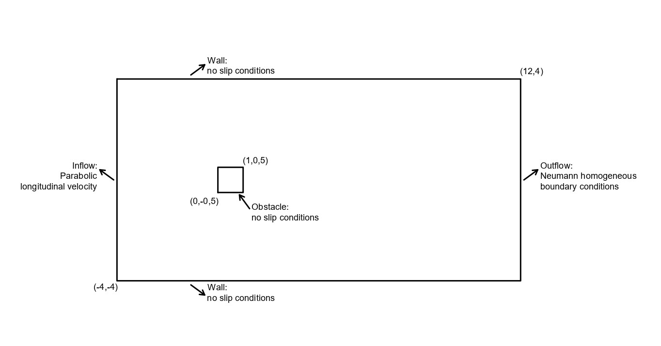
Figure 1: Domain of interest with the boundary conditions of the fluid-dynamics test case

We will use both manufactured (i.e., analytical) solutions to monitor the decay of the true error and the estimator, and the (unknown) solution of a fluid-dynamics problem to investigate the effect of mesh-refinement driven by our estimator.

All our meshes are obtained by uniform or adaptive refinements from an initial, uniform partition of the domain into squares with edges equal to half the edge of the square cylinder. The classical quad-tree refinement is applied to each refined square, which replaces it by four equal sub-squares; this may generate hanging nodes. Following the VEM philosophy, a square containing hanging nodes is viewed as a polygon. For easiness of implementation, we confine ourselves to refinements with a maximum of one hanging node per edge (although from the theoretical point of view we could choose any bound for the maximum number of hanging nodes per edge). Thus, our VEM elements may range from pentagons (squares with one hanging node) to octagons (squares with four hanging nodes).

In some of the forthcoming plots, we will monitor the different components of the a posteriori estimator, which will be denoted by $\eta_{s}$ with

$$\eta_{s}^{2}=\sum_{E\in\mathcal{T}_{h}}\eta_{s,E}^{2}\,,$$ (50)

where the subscript $s$ stands for one of the subscripts previously used in the definition (28). We point out that we will enforce non-homogeneous Dirichlet boundary conditions and homogeneous Neumann boundary conditions, namely

$$\begin{cases}\mathbf{u}=\mathbf{g}\quad\text{on}\quad\partial\Omega_{D}\,,\\ (\nu\mathbf{\nabla}\mathbf{u}+p\mathbf{I})\mathbf{n}=\mathbf{0}\quad\text{on}\quad\partial\Omega_{N}\,,\\ \end{cases}$$ (51)

even if in Sect. 4.3 the estimator was defined assuming homogeneous Dirichlet boundary conditions only. The extension to the general case poses no difficulty.

The code used for implementation was written in Matlab, taking inspiration from Sutton (2017) and Beirão da Veiga et al. (2014).

In the following subsections we will briefly describe Newton’s method to solve the nonlinear problem, and the adaptive refinement algorithm. The last part of the section is devoted to the computational results.

5.1 Newton’s method

To solve the discrete Navier-Stokes equations (11), we used Newton’s method as described in Gunzburger and Peterson (1991). Starting from an initial guess $\mathbf{u}_{0}\in\mathbf{V}_{h}$, the Newton iterates $\{\mathbf{u}_{m}\in\mathbf{V}_{h},p_{m}\in Q_{h}\}_{m=1,2,...}$ are defined by

$$\begin{split}a_{h}(\mathbf{u}_{m},\mathbf{v}_{h})+{c}_{h}(\mathbf{u}_{m},\mathbf{u}_{m-1},\mathbf{v}_{h})+{c}_{h}(\mathbf{u}_{m-1},\mathbf{u}_{m},\mathbf{v}_{h})+b(\mathbf{v}_{h},p_{m})+b(\mathbf{u}_{m},q)\\ =(\mathbf{f}_{h},\mathbf{v}_{h})+{c}_{h}(\mathbf{u}_{m-1};\mathbf{u}_{m-1},\mathbf{v}_{h})\quad\forall\,\mathbf{v}_{h}\in\mathbf{V}_{h},q\in Q_{h}\,.\end{split}$$ (52)

The initial guess $\mathbf{u}_{0}$ is chosen as the solution of the corresponding Stokes problem, obtained as described in Beirão da Veiga et al. (2017). As a stopping rule, we impose the condition $\|\bar{\mathbf{u}}_{m}-\bar{\mathbf{u}}_{m-1}\|_{\ell_{2}}<\textit{tol}$, where $\bar{\mathbf{u}}_{m}$ is the array containing the values of the degrees of freedom of ${\mathbf{u}}_{m}$. The tolerance tol is a small arbitrary value chosen equal to $10^{-9}$. The maximum number of iterates is taken equal to $10$.

5.2 Refinement algorithm

The algorithm used to refine the mesh $\mathcal{T}_{h}$ was the classical $\texttt{SOLVE}\rightarrow\texttt{ESTIMATE}\rightarrow\texttt{MARK}\rightarrow\texttt{REFINE}$ loop. The subset of marked elements ${\cal M}_{h}$ is chosen according to Dörfler’s recipe

$$\sum_{E\in{\mathcal{M}_{h}}}\eta_{E}^{2}\geq\theta\sum_{E\in{\mathcal{T}_{h}}}\eta_{E}^{2}\,,$$ (53)

for some fixed $\theta\in(0,1)$. It is important to underline that, generally, the previous rule might produce meshes with an arbitrary number of hanging nodes per edge. Therefore, we implemented an additional recursive refinement procedure to satisfy the constraint of having at most one hanging node per edge.

5.3 Numerical tests with analytical solutions

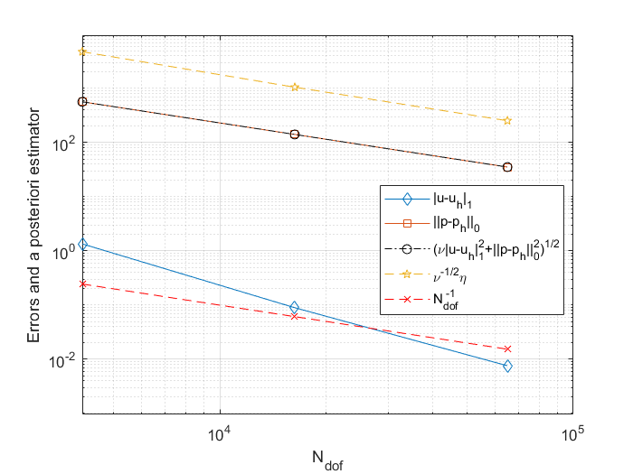
(a) $Re$=1

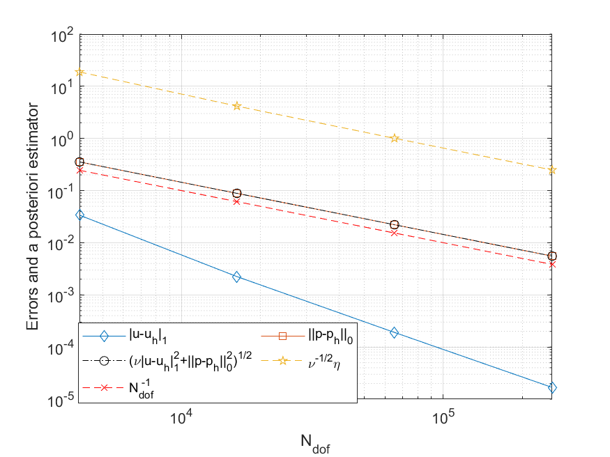
(b) $Re$=40

Figure 2: Test 1. Uniform refinements: errors and a posteriori estimator

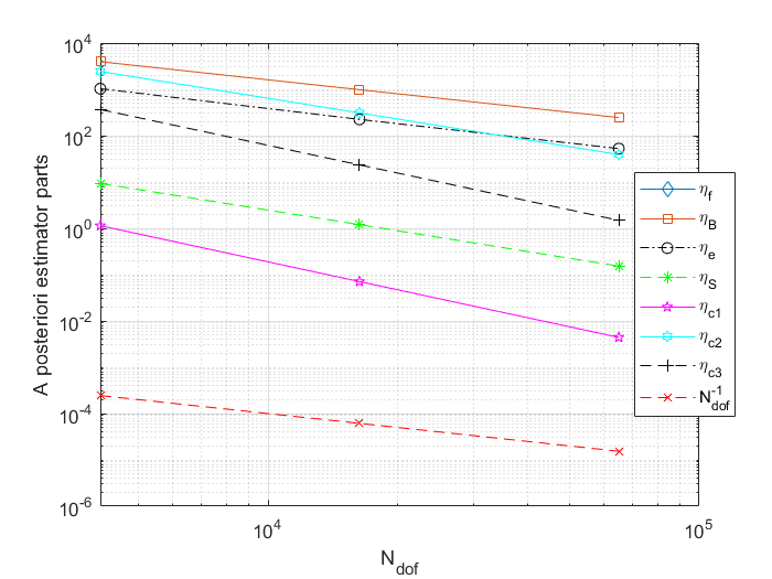
(a) $Re$=1

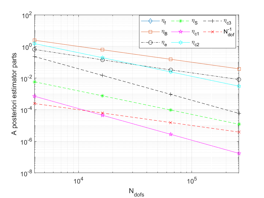
(b) $Re$=40

Figure 3: Test 1. Components of the a posteriori estimator during uniform refinements

Hereafter we report the results of some numerical experiments with manufactured solutions. We underline that in the plots related to velocity errors, we indicate such errors as $|\mathbf{u}-\mathbf{u}_{h}|_{1}$ but we actually mean $\left(\sum_{E\in\mathcal{T}_{h}}\|\mathbf{\nabla}\mathbf{u}-\mathbf{\Pi}^{0,E}_{1}\mathbf{\nabla}\mathbf{u}_{h}\|^{2}_{0,E}\right)^{1/2}$, since the explicit expression of the VEM solution is not known.

5.3.1 Test 1

Taking inspiration from Beirão da Veiga et al. (2018), we choose the following solution:

$$\mathbf{u}=\nu\begin{bmatrix}3(x^{2}-y^{2})\\ -2xy\end{bmatrix}\,,\qquad p=\nu^{2}(\frac{9}{2}(x^{2}+y^{2})^{2}-C)\,,$$ (54)

where $C=\int_{\Omega}\frac{9}{2}(x^{2}+y^{2})^{2}\,d\Omega/|\Omega|$. Dirichlet boundary conditions equal to the values of exact solution are enforced on $\partial\Omega$. With this solution one has $\mathbf{f}=\mathbf{0}$, which implies $\eta_{f}=0$. We applied uniform refinements of the initial mesh for different values of $Re$. In Figure 2 we show, in log-log scale, the behavior of the errors and the estimator for $Re=1$ and $Re=40$ vs the number of active degrees of freedom, whereas in Figure 3 we show the different components of the a posteriori estimator. We notice that the bulk error $\eta_{B}$ is the dominant one. We underline that the estimator and the pressure error follow the optimal convergence rate (indicated by the dashed line with symbol $\text{N}_{\text{dof}}^{-1}$), whereas the velocity error seems to decrease faster while adding degrees of freedoms. Note that the values of the estimator and the error in the case $Re=1$ are higher than the corresponding values for $Re=40$, simply because the exact solution is larger in the former case than in the latter. In this test Newton’s method converges in 3 iterations or less.

5.3.2 Test 2

We now consider the $\nu$-independent solution

$$\mathbf{u}=\begin{bmatrix}e^{-(x-12)/6}\sin(y/6)\\ -e^{-(x-12)/6}\cos(y/6)\end{bmatrix}\,,\qquad p=e^{(-(x-12)/6)}\sin(y/6)\,,$$ (55)

which satisfies $\nu\boldsymbol{\Delta}u=\mathbf{0}$, whence $\mathbf{f}=(\boldsymbol{\nabla}\mathbf{u})\mathbf{u}-\nabla p$. As in Test 1, we enforce Dirichlet conditions on $\partial\Omega$ and we use uniform mesh refinements.

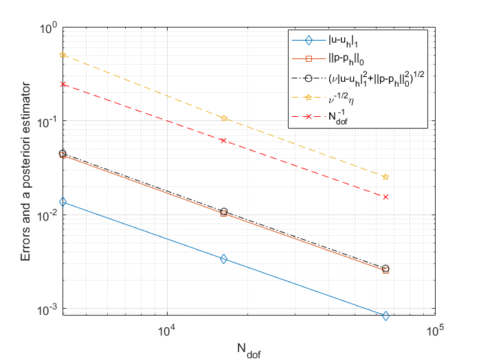
(a) $Re$=1

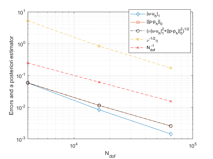
(b) $Re$=40

Figure 4: Test 2. Errors and a posteriori estimator during uniform refinements

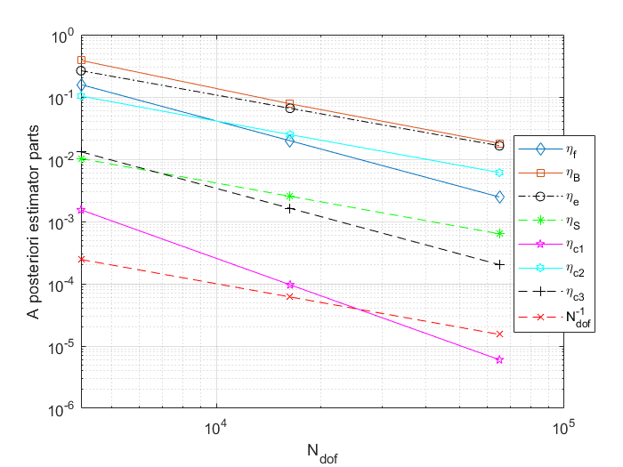
(a) $Re$=1

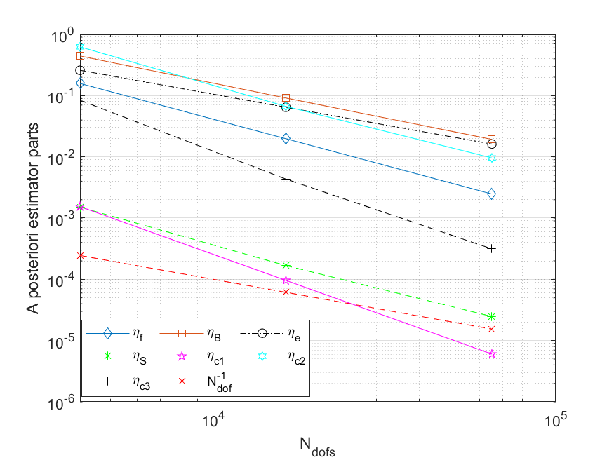
(b) $Re$=40

Figure 5: Test 2. Components of the a posteriori estimator during uniform refinements

In Figure 4 we report the errors and the a posteriori estimator vs the number of active degrees of freedom, while in Figure 5 we report the various components of the a posteriori estimator, considering two cases with $Re=1$ and $Re=40$. We see that in this test $\eta_{f}$ is different from $0$ but decreases fast. Furthermore, we notice that for $Re=1$ the dominant part is again the bulk error, whereas for $Re=40$ at the beginning the dominant part is $\eta_{c2}$, then again $\eta_{B}$ becomes the most important one. Again, Newton’s method converges in 3 iterations or less. Overall, velocity and pressure errors as well as the estimator scale according to the optimal convergence rate.

5.4 Fluid dynamics case

The fluid dynamics case describes the flow around a square cylinder in a channel, following the setting in Breuer et al. (2000). There is no external forces, so $\mathbf{f}=\mathbf{0}$. At the inflow we consider a parabolic velocity profile in the $x$-component:

$$\mathbf{u}_{I}=\begin{bmatrix}-1/16(y-4)(y+4)\\ 0\end{bmatrix}\,.$$ (56)

No slip conditions ($\mathbf{u}=\mathbf{0}$) are enforced on the cylinder and channel walls, whereas homogeneous Neumann conditions are chosen at the outflow. The problem is adimensionalized with the maximum inflow velocity as characteristic velocity.

We apply in this case an adaptive refinement with Dörfler parameter $\theta=0.4$. In Figure 6 we report the estimator and its components vs the number of active degrees of freedom, when $Re=30$: we observe that all monitored quantities decrease very fast at the beginning, while later they follow the expected convergence. We also show in Figure 7 some meshes produced by the refinement, and in Figure 8 some velocity fields, where the blue lines represent Matlab-generated approximate streamlines. One may appreciate the refinement around the cylinder, in particular around its corners pointing towards the inflow side, as we can see from Figure 7(c). Indeed, the refinement becomes, as the Reynolds number increases, more and more non-symmetric with respect to the vertical axis $x=1/2$ passing through the center of the cylinder (whereas in the Stokes case the refined meshes are symmetric in the flow direction). The refinement is concentrated about the upstream edge of the cylinder as $Re$ increases, while there is less refinement near the downstream edge.

In the current situation, we observe the appearance of recirculation eddies past the cylinder (see Figure 8(c)), whose length (the recirculation length) can be estimated by linear interpolation, after identifying the element edge on the line $y=0$ where $u_{x}$ (the x-component of $\mathbf{u}$) changes sign past the cylinder. The computed values of the recirculation length for different Reynolds numbers are reported in Table 1; they exhibit a linear growth, which is in good agreement with analogous results in the literature (see Breuer et al. (2000)). Note that in the recirculation area we do not see a strong refinement; this can be related to the presence of very low values of velocity therein.

Table 1: Recirculation length for different Reynolds numbers

Re	10	15	20	25	30	35	40	45	50	55
Recir. Len.	1.50	1.79	2.09	2.39	2.70	3.00	3.29	3.58	3.79	4.15

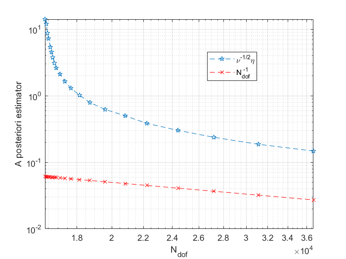
(a) A posteriori estimator

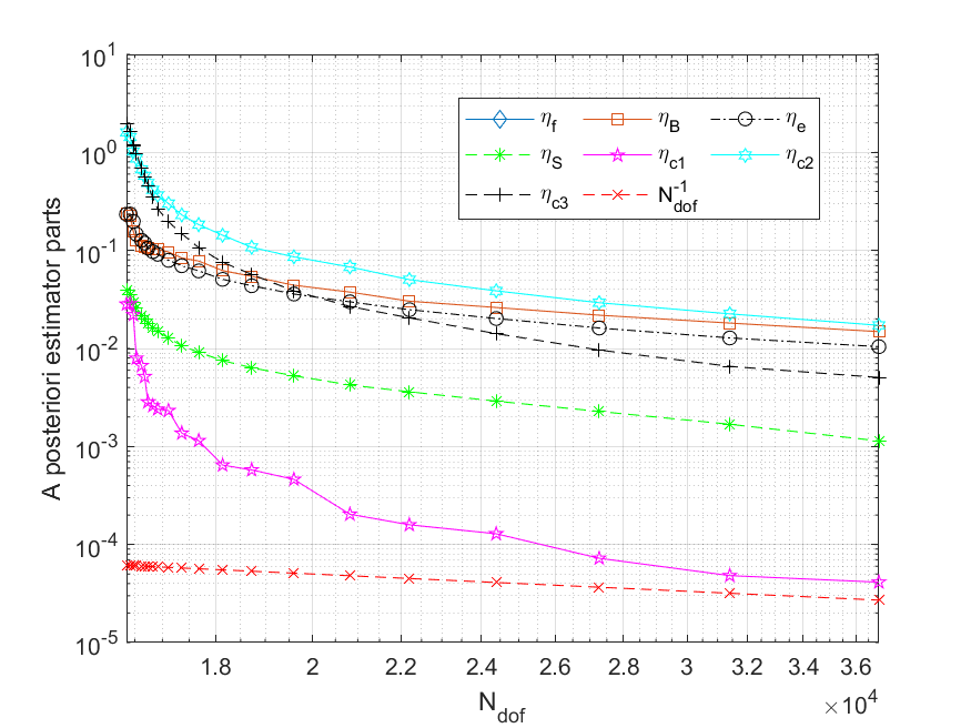
(b) Components of the estimator

Figure 6: Fluid dynamics case. A posteriori estimator (left) and its components (right) for $Re=30$

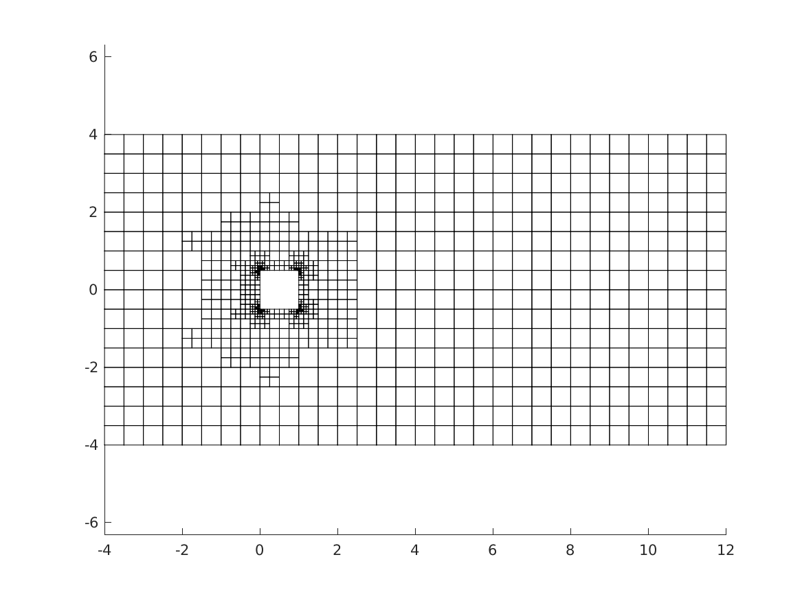
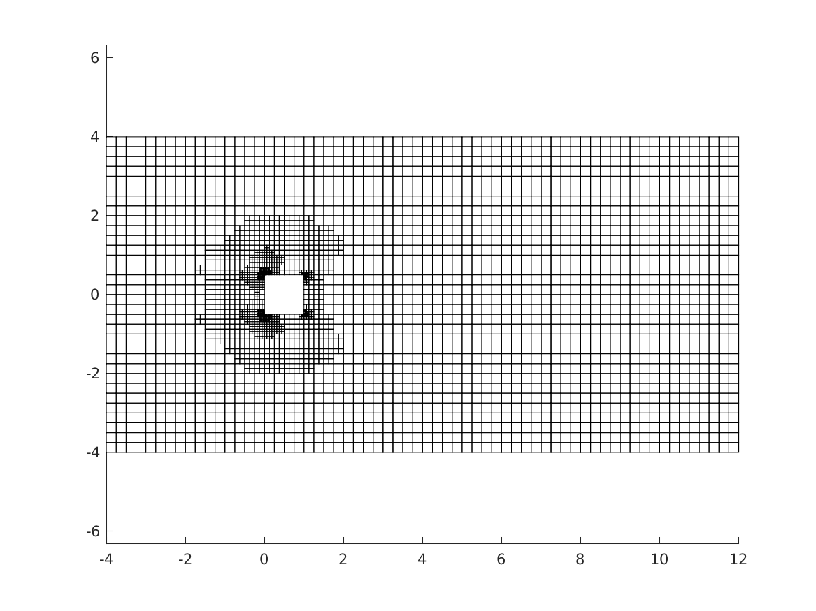
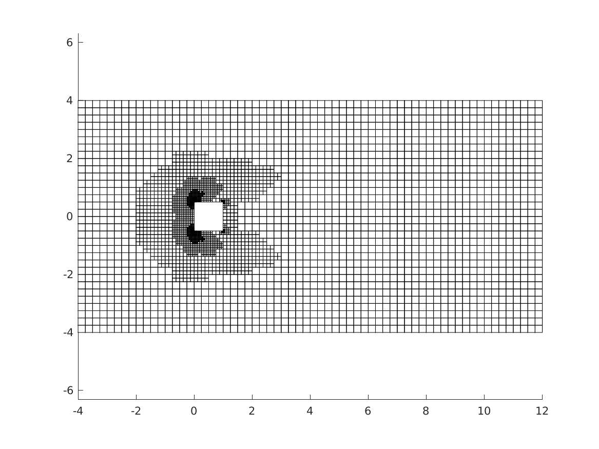
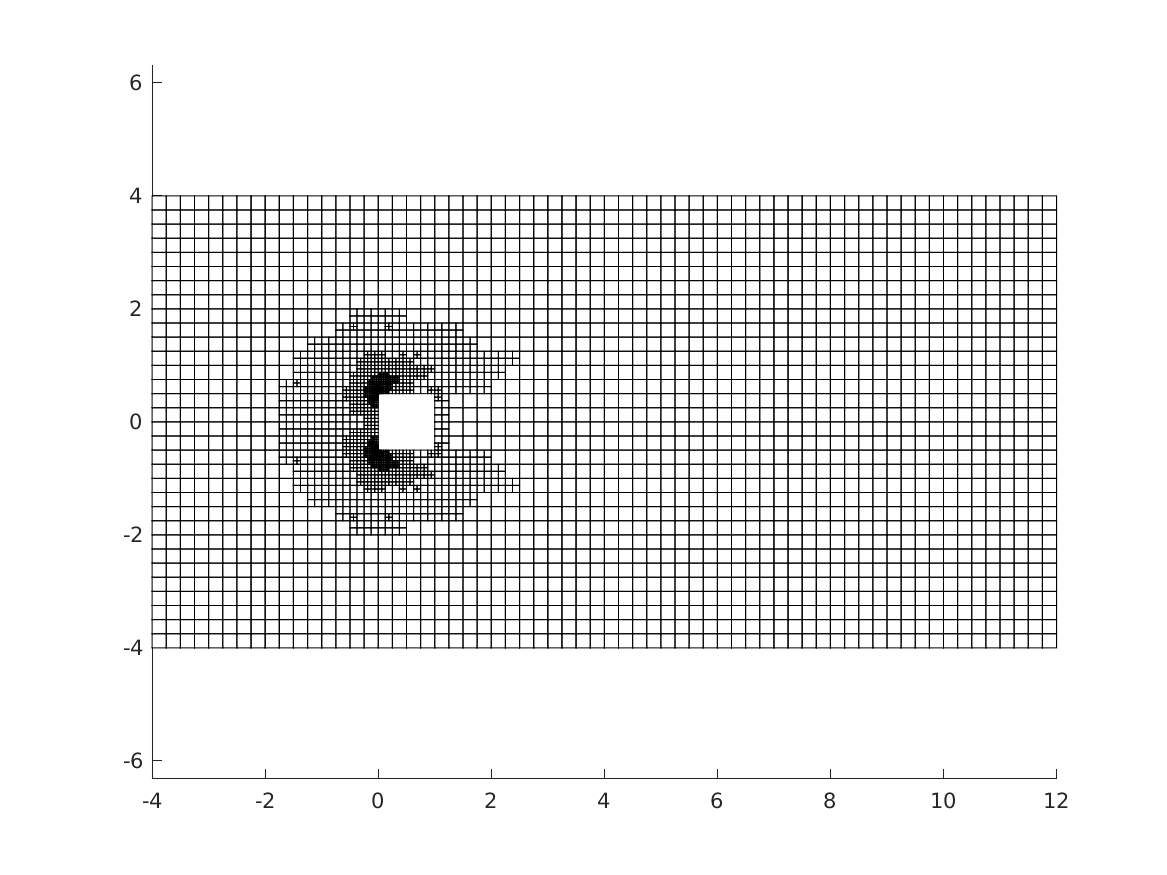
(a) $Re$=1 (10 steps) (b) $Re$=10 (15 steps) (c) $Re$=30 (20 steps) (d) $Re$=50 (20 steps)

Figure 7: Flow around a square cylinder. Meshes at the end of the adaptive refinement for different Reynolds numbers. ‘Steps’ indicates the number of steps performed in the refinement loop

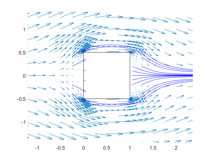
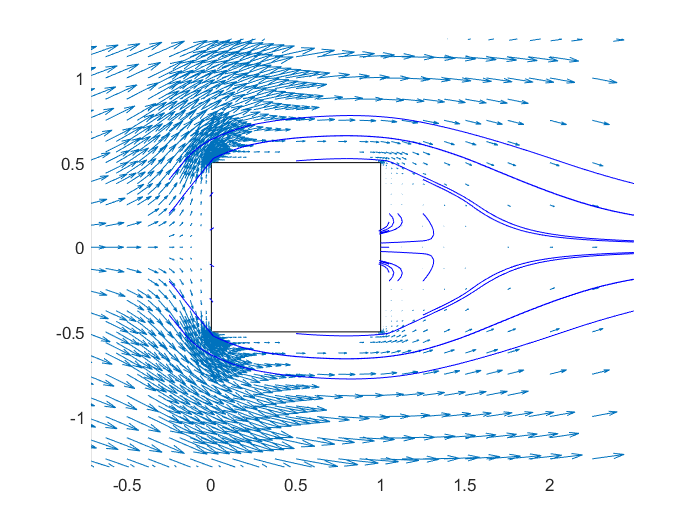
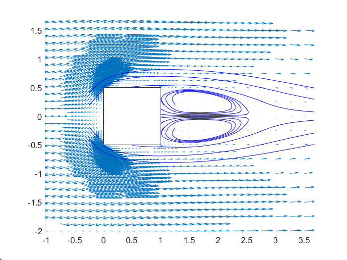
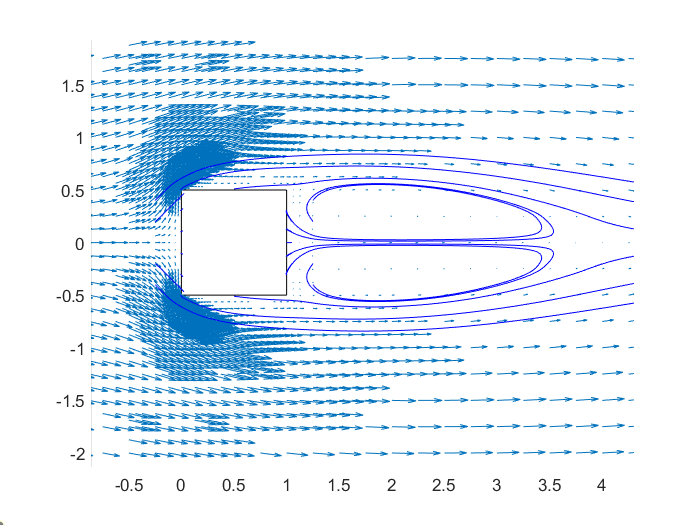
(a) $Re$=1 (b) $Re$=10 (c) $Re$=30 (d) $Re$=50

Figure 8: Flow around a square cylinder. Velocity fields and streamlines, computed on the corresponding meshes given in Figure 7

6 Conclusions

In this work we considered the divergence-free Virtual Element Method proposed in Beirão da Veiga et al. (2018) for the numerical solution of the steady incompressible Navier-Stokes equations. The method is of arbitrary order $k\geq 2$, meaning that the local VEM space approximates velocities on the boundary of the mesh element by piecewise polynomials of degree $k$, whereas pressures are locally approximated by polynomials of degree $k-1$.

• We defined a residual-based a posteriori estimator for a linear combination of the $H^{1}$-seminorm error on velocity and the $L^{2}$-norm error on pressure.

• We established the reliability of the new estimator, proving that it provides an upper bound for this error. Furthermore, we highlighted the origin of the different components of the estimator.

• With respect to the Stokes case, in addition to a different definition of the bulk error, our estimator includes three new terms originated by the VEM discretization of the nonlinear convective term.

• We derived lower bounds for the error, which involve all the terms in the estimator and indicate that the proposed estimator is also efficient.

• We performed some numerical tests with order $k=2$ and uniform mesh refinement, showing the correct rate of decay of the estimator and its control over the true errors. We also highlighted the behaviour of the various components of the estimator.

• Finally, we applied an adaptive mesh refinement based on the new estimator to the flow around a square obstacle in the stationary and laminar regime $Re<60$. Our results are in good agreement with classical results obtained by finite-volume simulations (see Breuer et al. (2000)); in particular, the recirculation lengths past the obstacle increase in agreement with Breuer et al. (2000). The refined meshes appear to fit the structures of the physical solution for simulations at different Reynolds numbers, showing a good performance of the new estimator.

Declarations

The authors have no relevant financial or non-financial interests to disclose.

This research was done in the framework of the Italian MIUR Award “Dipartimenti di Eccellenza 2018-2022" granted to the Department of Mathematical Sciences, Politecnico di Torino (CUP: E11G18000350001). CC is a member of the Italian INdAM-GNCS research group and was supported by the MIUR PRIN Project 201752HKH8-003.

References

- Beirão da Veiga et al. [2013] L. Beirão da Veiga, F. Brezzi, A. Cangiani, G. Manzini, L. D. Marini, and A. Russo. Basic principles of virtual element methods. Math. Models Methods Appl. Sci., 23(01):199–214, 2013. doi:10.1142/S0218202512500492. URL https://doi.org/10.1142/S0218202512500492.
- Beirão da Veiga et al. [2014] L. Beirão da Veiga, F. Brezzi, L. D. Marini, and A. Russo. The hitchhiker’s guide to the virtual element method. Math. Models Methods in Appl. Sci., 24(08):1541–1573, 2014. doi:10.1142/S021820251440003X. URL https://doi.org/10.1142/S021820251440003X.
- Beirão da Veiga et al. [2017] L. Beirão da Veiga, C. Lovadina, and G. Vacca. Divergence free virtual elements for the Stokes problem on polygonal meshes. ESAIM: M2AN, 51(2):509–535, 2017. doi:10.1051/m2an/2016032. URL https://doi.org/10.1051/m2an/2016032.
- Beirão da Veiga et al. [2018] L. Beirão da Veiga, C. Lovadina, and G. Vacca. Virtual elements for the Navier–Stokes problem on polygonal meshes. SIAM Journal on Numerical Analysis, 56(3):1210–1242, 2018. doi:10.1137/17M1132811. URL https://doi.org/10.1137/17M1132811.
- Wang et al. [2020] G. Wang, Y. Wang, and Y. He. A posteriori error estimates for the virtual element method for the Stokes problem. Journal of Scientific Computing, 84(37), 2020. doi:10.1007/s10915-020-01281-2. URL https://doi.org/10.1007/s10915-020-01281-2.
- Wang et al. [2021] Ying Wang, Gang Wang, and Feng Wang. An adaptive virtual element method for incompressible flow. Computers & Mathematics with Applications, 101:63–73, 2021. ISSN 0898-1221. doi:https://doi.org/10.1016/j.camwa.2021.09.012. URL https://www.sciencedirect.com/science/article/pii/S0898122121003394.
- Beirão da Veiga et al. [2021a] L. Beirão da Veiga, C. Canuto, R. H. Nochetto, and G. Vacca. Equilibrium analysis of an immersed rigid leaflet by the virtual element method. Math. Models Methods Appl. Sci., 31(7):1323–1372, 2021a.
- Beirão da Veiga et al. [2021b] L. Beirão da Veiga, C. Canuto, R. H. Nochetto, G. Vacca, and M. Verani. Adaptive VEM: stabilization-free a posteriori error analysis and convergence property, 2021b. URL https://arxiv.org/abs/2111.07656.
- Breuer et al. [2000] M. Breuer, J. Bernsdorf, T. Zeiser, and F. Durst. Accurate computations of the laminar flow past a square cylinder based on two different methods: lattice-Boltzmann and finite-volume. International Journal of Heat and Fluid Flow, 21(2):186–196, 2000. ISSN 0142-727X. doi:https://doi.org/10.1016/S0142-727X(99)00081-8. URL https://www.sciencedirect.com/science/article/pii/S0142727X99000818.
- Cangiani et al. [2017] A. Cangiani, E.H. Georgoulis, T. Pryer, and O. J. Sutton. A posteriori error estimates for the virtual element method. Numer. Math., 137:857–893, 2017. doi:10.1007/s00211-017-0891-9. URL https://doi.org/10.1007/s00211-017-0891-9.
- Ainsworth and Oden [1997] Mark Ainsworth and J.Tinsley Oden. A posteriori error estimation in finite element analysis. Computer Methods in Applied Mechanics and Engineering, 142(1):1–88, 1997. ISSN 0045-7825. doi:https://doi.org/10.1016/S0045-7825(96)01107-3. URL https://www.sciencedirect.com/science/article/pii/S0045782596011073.
- Vacca [2018] Giuseppe Vacca. An H1-conforming virtual element for Darcy and Brinkman equations. Mathematical Models and Methods in Applied Sciences, 28(01):159–194, 2018. doi:10.1142/S0218202518500057. URL https://doi.org/10.1142/S0218202518500057.
- Verfürth [1996] R. Verfürth. A Review of A Posteriori Error Estimation and Adaptive Mesh-Refinement Techniques. Wiley Teubner, Stuttgart, 1996.
- Kanschat and Schötzau [2008] Guido Kanschat and Dominik Schötzau. Energy norm a posteriori error estimation for divergence-free discontinuous Galerkin approximations of the Navier-Stokes equations. Internat. J. Numer. Methods Fluids, 57(9):1093–1113, 2008. doi:10.1002/fld.1795. URL https://doi.org/10.1002/fld.1795.
- Sutton [2017] Oliver J. Sutton. The virtual element method in 50 lines of MATLAB. Numer Algor, 75:1141–1159, 2017. doi:10.1007/s11075-016-0235-3. URL https://doi.org/10.1007/s11075-016-0235-3.
- Gunzburger and Peterson [1991] Max D. Gunzburger and Janet S. Peterson. Predictor and steplength selection in continuation methods for the Navier-Stokes equations. Computers & Mathematics with Applications, 22(8):73–81, 1991. ISSN 0898-1221. doi:https://doi.org/10.1016/0898-1221(91)90015-V. URL https://www.sciencedirect.com/science/article/pii/089812219190015V.