Coherence generation, symmetry algebras and Hilbert space fragmentation

Abstract

Hilbert space fragmentation is a novel type of ergodicity breaking in closed quantum systems. Recently, an algebraic approach was utilized to provide a definition of Hilbert space fragmentation characterizing families of Hamiltonian systems based on their (generalized) symmetries. In this paper, we reveal a simple connection between the aforementioned classification of physical systems and their coherence generation properties, quantified by the coherence generating power (CGP). The maximum CGP (in the basis associated to the algebra of each family of Hamiltonians) is exactly related to the number of independent Krylov subspaces $K$, which is precisely the characteristic used in the classification of the system. In order to gain further insight, we numerically simulate paradigmatic models with both ordinary symmetries and Hilbert space fragmentation, comparing the behavior of the CGP in each case with the system dimension. More generally, allowing the time evolution to be any unitary channel in a specified algebra, we show analytically that the scaling of the Haar averaged value of the CGP depends only on $K$. These results illustrate the intuitive relationship between coherence generation and symmetry algebras.

I Introduction

Non-equilibrium quantum dynamics of closed systems has been an extensively studied issue in recent years. Generic isolated quantum systems are expected to thermalize in the thermodynamic limit, in the sense that for any small subsystem the rest of the system acts as a bath, so that the expectation value of local observables coincides with that derived by statistical mechanical ensembles Nandkishore and Huse (2015); Gogolin and Eisert (2016). A central role in the understanding of this phenomenon is played by the so-called eigenstate thermalization hypothesis (ETH) Deutsch (1991); Srednicki (1994); Rigol et al. (2008), according to which, under certain conditions, the energy eigenstates are conjectured to be thermal, i.e. the expectation values of observables with local support over the energy eigenstates coincide with those of a thermal ensemble with temperature related to the energy D’Alessio et al. (2016).

While ETH is expected to hold for generic systems Rigol et al. (2008); Rigol and Santos (2010); Ikeda et al. (2011); Dubey et al. (2012); Steinigeweg et al. (2013); Kim et al. (2014); Beugeling et al. (2014); Steinigeweg et al. (2014); Müller et al. (2015); Mondaini et al. (2016), several ETH-violating classes of models are known. Integrable systems and many-body localized (MBL) systems are the two prime examples, where an extensive number of conserved quantities prevent the system from thermalizing. The conserved quantities are a result of symmetries readily encoded in the Hamiltonian (in the integrable systems) or from emergent symmetries created by strong disorder (in the MBL case). More novel types of disorder-free ergodicity breaking models were recently observed and studied, dubbed quantum many-body scars (QMBS) Bernien et al. (2017); Shiraishi and Mori (2017); Turner et al. (2018a, b); Moudgalya et al. (2018a); Lin and Motrunich (2019); Ok et al. (2019); Pai and Pretko (2019); Mark et al. (2020); Hudomal et al. (2020); Iadecola and Vijay (2020); Iadecola and Schecter (2020); McClarty et al. (2020); Langlett and Xu (2021); Papaefstathiou et al. (2020); Desaules et al. (2021); Moudgalya et al. (2020a); Banerjee and Sen (2021); Lee et al. (2020); Lin et al. (2020); Schecter and Iadecola (2019); Mark and Motrunich (2020); Pakrouski et al. (2020); Moudgalya et al. (2020b); Moudgalya and Motrunich (2022a) and Hilbert space fragmentation Khemani et al. (2020); Sala et al. (2020); Yang et al. (2020); Rakovszky et al. (2020); Herviou et al. (2021); Hahn et al. (2021); Langlett and Xu (2021); Moudgalya et al. ; De Tomasi et al. (2019); Lee et al. (2021); Karpov et al. (2021); Zhang and Røising (2022); Khudorozhkov et al. (2022); Moudgalya and Motrunich (2022b). QMBS correspond to a weak violation of ETH, in which only a small set of eigenstates in the bulk of the spectrum are non-thermal. Emergence of scar dynamics has been linked with the existence of dynamical symmetries Medenjak et al. (2020); Pakrouski et al. (2020); O’Dea et al. (2020); Ren et al. (2021), that allow the formation of towers of scar eigenstates inside an invariant subspace. Hilbert space fragmentation corresponds to the broader phenomenon of "shattering" of the Hilbert space in exponentially many dynamically disconnected subspaces (referred to as Krylov subspaces) with no obvious associated conserved quantities. In addition to weak violation, such systems can exhibit a strong violation of ETH, where a nonzero measure subset of all the eigenstates is non-thermal.

Recently, an algebraic framework was utilized to analyze the phenomenon of Hilbert space fragmentation for families of Hamiltonians Moudgalya and Motrunich (2022b), establishing the role of non-conventional symmetries. Such an approach reveals the central role of the symmetry algebra in the classification of the system, and is applicable to conventional models as well Moudgalya and Motrunich (2022c). Another inherent advantage is that the properties exhibited by the families of Hamiltonians are free from fine-tuning. In general, systems exhibiting novel ergodic behavior (such as QMBS and Hilbert space fragmentation) belong to special classes of Hamiltonians Moudgalya and Motrunich (2022b) that are of great interest in attempts to fully describe the behavior of non-equilibrium closed quantum systems Sala et al. (2020); Moudgalya et al. (2018a, b); Iadecola and Žnidarič (2019); Iadecola et al. (2019); Ok et al. (2019).

The ergodic properties of a system are correlated with information-theoretic signatures, such as eigenstate entanglement Khare and Choudhury (2020); noa (a); Papić (2022) and information scrambling Sun et al. (2021); Yuan et al. (2022); Turner et al. (2018a). In this paper, we establish a connection between the classification framework introduced in Moudgalya and Motrunich (2022b) and coherence, quantified by the coherence generating power (CGP) Zanardi et al. (2017a, b); Zanardi and Campos Venuti (2018); Styliaris et al. (2018). The CGP bound established in this paper becomes particularly relevant for the aforementioned special classes of Hamiltonians exhibiting Hilbert space fragmentation.

This paper is structured as follows. In Section II, we present an analytical upper bound of the CGP of families of Hamiltonian evolutions, with respect to a basis induced by the algebra of each family; this bound is fully described by the aforementioned classification of the families of Hamiltonians. We, also, provide numerical results of systems with both ordinary symmetries and Hilbert space fragmentation and compare the behavior of the CGP as we increase the system size. In Section III, we allow the evolution to be any unitary channel in a prescribed algebra and show that the Haar average value of the CGP is typical and its scaling with the system size is fully described by the classification of unitary evolutions in the algebra. In Section IV, we conclude with a brief discussion of the results. The detailed proofs of the analytical results are included in the Supplemental Material A.

II Coherence generating power for classes of models

II.1 Preliminaries

Let $\mathcal{H}\cong\mathbb{C}^{d}$ be a finite $d$-dimensional Hilbert space and denote the space of linear operators acting on it as $\mathcal{L}(\mathcal{H})$. The key mathematical structures of interest are $*$-closed untial algebras of observables $\mathcal{A}$, alongside their commutants,

$$\mathcal{A}^{\prime}=\{Y\in\mathcal{L}(\mathcal{H})\;|\;[X,Y]=0\;\forall\;X\in\mathcal{A}\}$$

Due to the double commutant theorem these algebras always come in pairs, so as $(\mathcal{A}^{\prime})^{\prime}=\mathcal{A}$ Davidson (1996).

Letting $\mathcal{Z}(\mathcal{A}):=\mathcal{A}\cap\mathcal{A}^{\prime}$ denote the center of $\mathcal{A}$ with $d_{\mathcal{Z}}:=\dim\mathcal{Z}(\mathcal{A})$, a fundamental structure theorem for $C^{*}$-algebras implies a decomposition of the Hilbert space of the form Davidson (1996)

$$\begin{split}&\mathcal{H}\cong\oplus_{J=1}^{d_{\mathcal{Z}}}\,\mathbb{C}^{n_{J}}\otimes\mathbb{C}^{d_{J}},\\ &\mathcal{A}\cong\oplus_{J=1}^{d_{\mathcal{Z}}}\,\mathds{1}_{n_{J}}\otimes\mathcal{L}(\mathbb{C}^{d_{J}}),\\ &\mathcal{A}^{\prime}\cong\oplus_{J=1}^{d_{Z}}\,\mathcal{L}(\mathbb{C}^{n_{J}})\otimes\mathds{1}_{d_{J}}.\end{split}$$ (1)

Due to the above decomposition,

$$\begin{split}&\dim\mathcal{H}\equiv d=\sum_{J=1}^{d_{\mathcal{Z}}}n_{J}d_{J},\\ &\dim\mathcal{A}=\sum_{J=1}^{d_{\mathcal{Z}}}d_{J}^{2}=:d(\mathcal{A}),\\ &\dim\mathcal{A}^{\prime}=\sum_{J=1}^{d_{\mathcal{Z}}}n_{J}^{2}=:d(\mathcal{A}^{\prime}).\end{split}$$

In general the algebra $\mathcal{A}^{\prime}$ is non-Abelian and we will denote as $\mathcal{M}\subset\mathcal{A}^{\prime}$ the (possibly not unique) maximal Abelian subalgebra of the commutant with dimension $K:=\dim\mathcal{M}=\sum_{J=1}^{d_{\mathcal{Z}}}n_{J}$. Note that $K$ is exactly the number of linearly independent common invariant subspaces of all operators in $\mathcal{A}$.

Given a basis $B=\{\ket{i}\}_{i=1}^{d}$ of $\mathcal{H}$, one can always express a pure state as a linear superposition of the states $\ket{i}$. This fact is experimentally materialized as what is called quantum coherence Glauber (1963). In general, one defines $B$-incoherent states $\rho$ ($\rho\geq 0,\Tr\rho=1$) as states diagonal in $B$ (coherent states are all states that are not incoherent). Given a unitary operator $U\in\mathcal{L}(\mathcal{H})$ a measure of its coherence generating power (CGP) with respect to the basis $B$ is given by Zanardi et al. (2017b)

$$C_{B}(U)=1-\frac{1}{d}\sum_{i,j=1}^{d}\lvert\matrixelement{i}{U}{j}\rvert^{4}$$ (2)

Note that the above quantity coincides with a measure of information scrambling of $B$-diagonal ("incoherent") degrees of freedom Zanardi ; Andreadakis et al. (2022), which aligns with its ability of quantifying the deviation of incoherent states from the incoherent space under evolution with $U$.

Ref. Moudgalya and Motrunich (2022b) introduced an algebra based classification of multi-site Hamiltonian models. Given an algebra $\mathcal{A}$ that can be generated by local operators $h_{j}$, one considers the family of Hamiltonians

$$H=\sum_{j}J_{j}\;h_{j}$$ (3)

where $J_{j}$ are arbitrary coupling constants. Then, the symmetries of the system are characterized by the scaling of $K$ with the system size. For example, for 1D systems of size $L$, if $\log K\sim L$, then the family of Hamiltonians in Eq. 3 possesses an exponentially large number of dynamically disconnected subspaces, which serves as the definition of Hilbert space fragmentation (see Table 1). The models exhibiting Hilbert space fragmentation were shown to exhibit nonlocal conserved quantities, dubbed as statistically localized integrals of motion (SLIOMs) Rakovszky et al. (2020); Moudgalya and Motrunich (2022b).

$\log K$	Class representative
$\sim\mathcal{O}(1)$	Discrete global symmetry
$\sim\log L$	Continuous global symmetry
$\sim L$	Fragmentation

Table 1: Classification of families Hamiltonians of the form Eq. 3 based on the scaling of the dimension $K$ of the maximally abelian subalgebra of the commutant $\mathcal{A}^{\prime}$ with system size $L$ in 1D.Moudgalya and Motrunich (2022b)

II.2 Coherence generating power bound

We consider an algebra $\mathcal{A}=\langle h_{j}\rangle$ and families of Hamiltonians of the form Eq. 3. Clearly, $H\in\mathcal{A}$ and due to Eq. 1

$$U:=\exp(-it\,H)=\oplus_{J=1}^{d_{\mathcal{Z}}}\mathds{1}_{n_{J}}\otimes U_{J}$$ (4)

We also consider a basis $B_{\mathcal{A}}=\{\ket{\phi_{J}}\otimes\ket{\psi_{J}}\;|\;J=1,\dots,d_{\mathcal{Z}},\;\phi_{J}=1,\dots,n_{J},\;\psi_{J}=1,\dots,d_{J}\}$, where $\ket{\phi_{J}}$ and $\ket{\psi_{J}}$ span $\mathbb{C}^{n_{J}}$ and $\mathbb{C}^{d_{J}}$ of the decomposition Eq. 1. We can, then, show that

Proposition 1.

1. The CGP of $U=\exp(-it\,H)\in\mathcal{A}$ in a basis $B_{\mathcal{A}}$ induced by the algebra decomposition is

   $$\begin{split}C_{B_{\mathcal{A}}}(U)&=1-\frac{1}{d}\sum_{J,\psi_{J},\psi^{\prime}_{J}}n_{J}\;\lvert\matrixelement{\psi_{J}}{U_{J}}{\psi^{\prime}_{J}}\rvert^{4}\\ &=:1-\frac{1}{d}f_{B_{\mathcal{A}}}(U)\end{split}$$ (5)

2. The maximum value of the CGP is

   $$\max_{U\in\mathcal{A}}C_{B_{\mathcal{A}}}(U)=1-\frac{1}{d}K$$ (6)

   and is achieved when $\lvert\matrixelement{\psi_{J}}{U_{J}}{\psi^{\prime}_{J}}\rvert=d_{J}^{-1/2}$ for all $J$.

We note that if $U$ is any unitary operator in $\mathcal{L}(\mathcal{H})$, then the maximum CGP is $C_{max}=1-\frac{1}{d}$ Zanardi et al. (2017b); Zanardi ; Andreadakis et al. (2022). The difference in the bound of Eq. 6 is an extra factor of $K$, which is exactly the number of independent common invariant subspaces for all evolutions generated by the family of Hamiltonians in Eq. 3. The scaling of $K$ with the system dimension provides a classification of this family (see e.g. Table 1), thus from Eq. 6 the scaling of the maximum CGP of the entire family of Hamiltonians is also dependent solely on this classification as well. This observation constitutes an exact, analytical implementation of the intuitive connection between (generalized) system symmetries and coherence generation. Note that the Hilbert space decomposition Eq. 1 is a basic element for the protection of quantum coherence in information processes, e.g. by decoherence-free subspaces and subsystems noa (b); Zanardi (1998); Lidar et al. (1998); noa (c). There, the algebra $\mathcal{A}$ is generated by the system operators of the interaction Hamiltonian and $K$ is simply the total dimension of decoherence-free subsystems $\mathbb{C}^{n_{J}}$.

II.3 Quantum spin-chain models

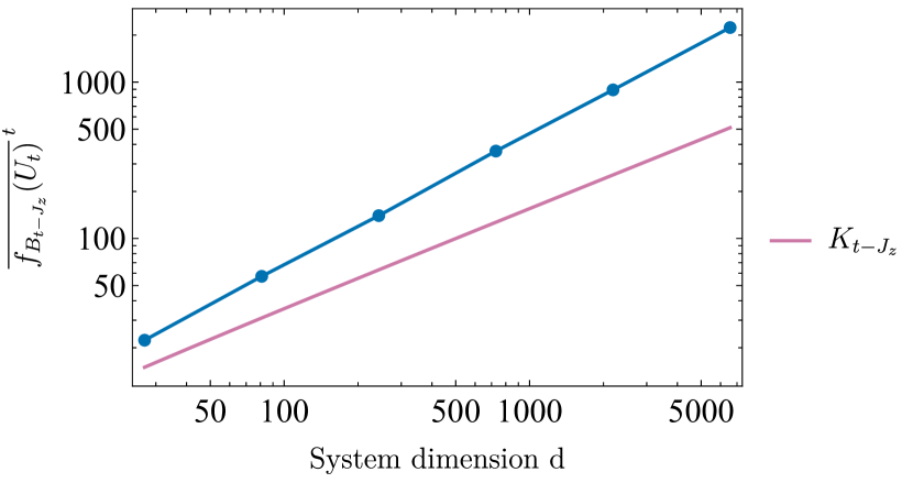
(a)

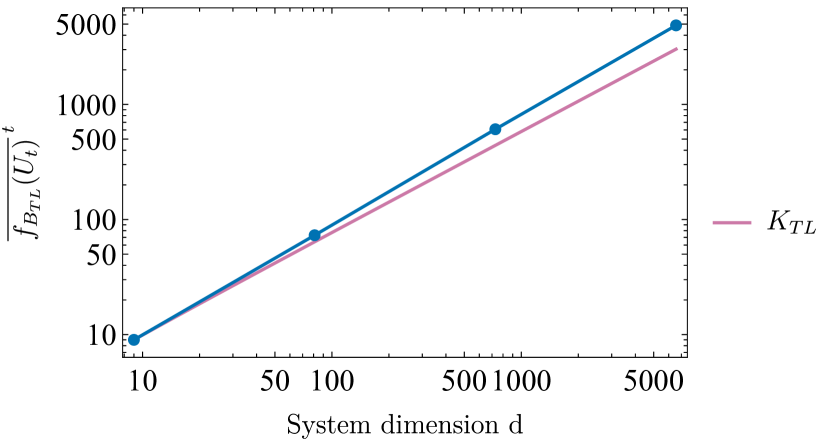
(b)

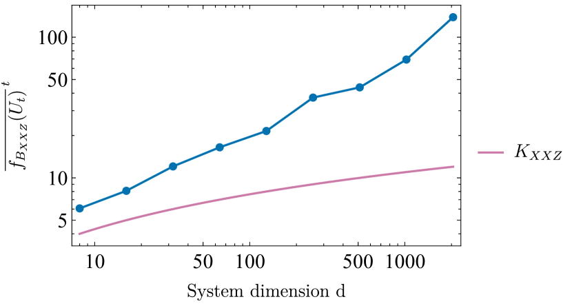
(c)

Figure 1: Log-log plots of long-time average of $f_{B_{\mathcal{A}}}(U)=1-C_{B_{\mathcal{A}}}(U)$ (connected dotted lines) in comparison to the bound $K$ (continuous lines) for: (a) the $t-J_{z}$ model; $\overline{f_{B_{t-J_{z}}}({U_{t}})}^{t}\sim d^{0.83}$ scales exponentially with the system size. The bound set by the number of independendent Krylov subspaces scales as $d^{\log_{3}2}$, (b) the $TL$ model; $\overline{f_{B_{TL}}({U_{t}})}^{t}\sim d^{0.95}$ scales exponentially with the system size. The scaling is very close to that set by the bound $d^{\log_{3}q}$ (see Section A.4), $\log_{3}q\simeq 0.88$, which can be understood in terms of the existence of Krylov-restricted thermalization in some of the large fragments of the $TL$ model Moudgalya et al. , (c) the $XXZ$ model; the behavior of $\overline{f_{B_{XXZ}}({U_{t}})}^{t}$ greatly deviates from the bound with the system size. Integrable systems (even with a random choice of couplings) are not expected to showcase generic properties, even after resolving for symmetries.

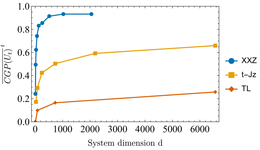
Figure 2: Comparison of the scaling of the CGP for the $XXZ$, $t-J_{z}$ and $TL$ models. We observe that for finite dimensions, the CGP of fragmented models is heavily constraint by the bound set in Eq. 6, leading to less mixing of different parts of the Hilbert space under evolution

Note that the result in Proposition 1 only depends on the fact that $U\in\mathcal{A}$ and not on the fact that $U$ is generated by a Hamiltonian of the form Eq. 3. As so, if we choose randomly a Hamiltonian from Eq. 3, the resulting evolution need not be typical. In order to evaluate the behavior of the CGP in such a case, we numerically simulate the evolution of spin-chain models in 1D with $L$ sites: (i) the spin-1/2 XXZ model with on-site magnetic field, (ii) the spin-1 Temperley-Lieb (TL) model, and (iii) the fermionic $t-J_{z}$ model.

$$\begin{split}&H_{XXZ}=\sum_{j}\left(J_{j}^{\perp}\left(\sigma_{j}^{x}\sigma_{j+1}^{x}+\sigma_{j}^{y}\sigma_{j+1}^{y}\right)+\right.\\ &\left.\hskip 65.0pt+J_{j}^{z}\sigma_{j}^{z}\sigma_{j+1}^{z}+h_{j}\sigma_{j}^{z}\right)\\ &H_{TL}=\sum_{j}J_{j}e_{j,j+1},\text{ where }e_{j,k}=3(\ket{\psi_{sing}}\bra{\psi_{sing}})_{j,k}\\ &\hskip 80.0pt\text{ and }\ket{\psi_{sing}}_{j,k}=\frac{1}{\sqrt{3}}\sum_{\alpha\in\{0,1,2\}}\ket{\alpha\alpha}_{j,k}\\ &H_{t-J_{z}}=\sum_{j}\left(-t_{j,j+1}\sum_{\sigma\in\{\uparrow,\downarrow\}}\left(\tilde{c}_{j,\sigma}\tilde{c}^{\dagger}_{j+1,\sigma}+h.c.\right)+\right.\\ &\left.\hskip 80.0pt+J_{j,j+1}^{z}S_{j}^{z}S_{j+1}^{z}+h_{j}S_{j}^{z}+g_{j}\left(S_{j}^{z}\right)^{2}\right),\\ &\hskip 50.0pt\text{where }S_{j}^{z}:=\tilde{c}_{j,\uparrow}^{\dagger}\tilde{c}_{j,\uparrow}-\tilde{c}_{j,\downarrow}^{\dagger}\tilde{c}_{j,\downarrow}\\ &\hskip 50.0pt\text{and }\tilde{c}_{j,\sigma}:=c_{j,\sigma}\left(1-c_{j,-\sigma}^{\dagger}c_{j,-\sigma}\right)\end{split}$$ (7)

Here, $\sigma_{j}^{\alpha},\alpha\in{x,y,z}$ denote the Pauli matrices. The XXZ model has shown to be integrable by Bethe ansatz Takahashi (1999) and possesses a conventional $U(1)$ symmetry with the associated conserved quantity $\sigma_{tot}^{z}=\sum_{j}\sigma_{j}^{z}$. The sectors of Eq. 1 are labeled by this conserved quantity ($J=L/2-\sigma_{tot}^{z}=0,\dots,L$) and the dimensions of the irreducible representations of $\mathcal{A}$ and $\mathcal{A}^{\prime}$ are $d_{J}={L\choose J}$ and $n_{J}=1$ respectively Moudgalya and Motrunich (2022b). For a given $J$ there is one common Krylov subspace (since $n_{J}=1$) and is spanned by the $z-basis$ product states with $\sigma_{tot}^{z}=L/2-J$). Note that $K_{XXZ}=L+1$, which scales linearly with the system size.

The TL model is an example of Hilbert space fragmentation. The dynamically disconnected Krylov subspaces are understood by the use of a basis of dots and non-crossing dimers Read and Saleur (2007); Batchelor and Barber (1990); Moudgalya and Motrunich (2022b). Each basis state consists of a pattern of dimers that connect two sites and represent the state $\ket{\psi_{sing}}_{j,k}$. The rest of the sites (that are not connected to either end of a dimer) make up the dots and the state $\ket{\psi_{dots}}$ is chosen such that it is annihilated by all projectors $\ket{\psi_{dim}}_{m,m+1}\bra{\psi_{dim}}_{m,m+1}$ (where $m$ labels all dots while excluding the dimers). The algebra formed by the $L-1$ generators $e_{j,j+1}$ is the Temperley-Lieb algebra $TL_{L}(q)$, where $q+q^{-1}=3$ (which is the number of local degrees of freedom in a spin-1 model)Moudgalya and Motrunich (2022b). It has been shown that, for even $L$, the sectors of the decomposition Eq. 1 are labeled by $J=0,\dots,L/2$ with corresponding dimensions

$$n_{J}=[2J+1]_{q},\;d_{J}={L\choose L/2+J}-{L\choose L/2+J+1}$$

where $[n]_{q}:=(q^{n}-q^{-n})/(q-q^{-1})$ is a $q$-deformed integer Read and Saleur (2007). It is, then, straightforward to show that $K=\frac{q^{-L}\left(q^{L+2}-1\right)^{2}}{\left(q^{2}-1\right)^{2}}$, which scales exponentially with the system-size.

The $t-J_{z}$ also falls into the category of Hilbert space fragmentation. The Hamiltonian acts effectively in the Hilbert space with no double occupancy and it has been shown that all operators in the commutant algebra are diagonal in the product state basisMoudgalya and Motrunich (2022b). The sectors are characterized by the pattern of spins $\uparrow$ and $\downarrow$, which remains invariant under the action of the HamiltonianRakovszky et al. (2020). For open boundary conditions (OBC) there are $2^{L+1}-1$ such sectors (all with $n_{J}=1$), so $K=2^{L+1}-1$ which scales exponentially with $L$Moudgalya and Motrunich (2022b).

We simulate exact dynamics for the above systems and for different system-sizes with the coupling constants randomly drawn from $[0,1]$ (each time we increase the system-size we add one more set of randomly chosen couplings to the previously drawn ones). The choice of the coupling constants sets the energy scale of the Hamiltonians, and in turn the timescale of the dynamics. For each model we construct the relevant bases described above and compute the long-time average of the CGP of the unitary evolution. In Fig. 1(a), 1(b) we observe that for the fragmented models the long-time average of the quantity $f_{B_{\mathcal{A}}}(U)$ (related to the CGP via Eq. 5) has a similar behavior with the number of Krylov subspaces $K$. Specifically, we find that (see also Section A.4)

$$\begin{split}&\overline{f_{B_{t-J_{z}}}({U_{t}})}^{t}\sim d^{0.83}\text{(compared to }K_{t-J_{z}}\sim d^{\log_{3}2})\\ &\overline{f_{B_{TL}}({U_{t}})}^{t}\sim d^{0.95}\text{ (compared to }K_{TL}\sim d^{\log_{3}q},\\ &\hskip 100.0pt\;q=(3+\sqrt{5})/2\simeq 2.62\text{)}\end{split}$$

Fragmented systems can be further characterized into strongly or weakly fragmented depending on the size $\max_{J}d_{J}$ of the biggest Krylov subspace; specifically for strongly (weakly) fragmented systems, $\max_{J}d_{J}/d\rightarrow 0$ ($\max_{J}d_{J}/d\rightarrow 1$) as $d\rightarrow\infty$ Sala et al. (2020); Moudgalya and Motrunich (2022b). When the size of the fragments is large enough (in the thermodynamic limit) and the Hamiltonian is non-integrable in these fragments, signatures of thermalization within the fragment can be observed, a phenomenon referred to as Krylov-restricted thermalization Moudgalya et al. . In fact, the $TL$ model has been shown to exhibit thermalization in some of its exponentially large Krylov subspaces Moudgalya et al. , which implies that the behavior of the CGP is expected to be closer to that of a generic model (see also Section III). In contrast to the fragmented models, the behavior of the CGP of the integrable $XXZ$ model with the system dimension is far away from the bound Eq. 6 (Fig. 1(c)). This aligns with the expectation that integrable models do not showcase features of generic evolutions, even after resolving for the symmetries. Fig. 2 emphasizes the vastly different CGP behaviors of the different classes of models simulated; for finite dimensions the bound Eq. 6 forces the CGP of the fragmented models to remain much lower than that of the integrable model. This shows that despite the fact that fragmented models are in general non-integrable, emergent generalized symmetries from kinetic constraints lead to a milder mixing of different parts of the Hilbert space, with possible physical importance for information processing tasks, e.g. protection of information via decoherence free subspaces Zanardi and Rasetti (1997a, b); Lidar et al. (1998) or utilization of (dynamical) localization for quantum memory implementations Hahn et al. (2021); Smith et al. (2016).

III Haar averaged coherence generating power and system-size scaling

We will now consider the case where $U\in\mathcal{A}$ can be any unitary in the algebra. It is straightforward to notice that Proposition 1 continues to hold, since Eq. 4 holds for all unitaries in the algebra. A natural question we wish to investigate is, given an algebra $\mathcal{A}$, what the typical value of the CGP is and how it is related to the number of independent Krylov subspaces $K$. To do so, we average $C_{B_{\mathcal{A}}}(U)$ over the Haar measure of the subgroup of unitaries $U\in\mathcal{A}$.

Proposition 2.

Given an algebra $\mathcal{A}$, the Haar average of the CGP over the unitaries in the algebra is

$$\overline{C_{B_{\mathcal{A}}}(U)}^{U\in\mathcal{A}}:={{\mathbb{E}}}_{U\in\mathcal{A}}\left[C_{B_{\mathcal{A}}}(U)\right]=1-\frac{1}{d}\sum_{J}\frac{2d_{J}}{d_{J}+1}\;n_{J}$$ (8)

Eq. 8 provides an analytical expression for the Haar average value of the CGP in terms of the dimensions $n_{J},\;d_{J}$ related to the decomposition Eq. 1. Since $1\leq d_{J}\leq d\;\forall J$ we can (loosely) bound the typical value as

$$1-\frac{2}{d+1}\;K\leq\overline{C_{B_{\mathcal{A}}}(U)}^{U\in\mathcal{A}}\leq 1-\frac{1}{d}\;K$$ (9)

This shows, that the scaling of the average value with the system dimension depends exactly on the classification of the model in terms of the scaling of $K$ with the system size (Section II.1). As seen in Proposition 4 of Zanardi et al. (2017b), Levy’s lemma implies that the Haar average is expected to be typical inside sufficiently large Krylov subspaces (see Section A.3). This aligns with the observation that the weakly fragmented $TL$ model seems to have close to maximal CGP, as in that case there is a dominant Krylov subspace, such that $\max_{J}\frac{d_{J}}{d}\rightarrow 1$ in the thermodynamic limit.

Note that due to the double commutant theorem, $\mathcal{A}$ is completely determined by the commutant $\mathcal{A}^{\prime}$, which represents the set of symmetries imposed on the evolution. As so, the selection of a random unitary in $\mathcal{A}$ corresponds to a random unitary channel constrained by physically motivated symmetries.

IV conclusion

In this paper we revealed a connection between a classification of families of Hamiltonian evolutions and their coherence generating power (CGP) with respect to a basis induced by the family. Specifically, the families of Hamiltonians were previously classified based on the scaling of the number $K$ of independent dynamically disconnected subspaces (called Krylov subspaces) with the system sizeMoudgalya and Motrunich (2022b). Each family of Hamiltonians is defined with respect to an algebra $\mathcal{A}$ generated by local terms that are used to compose the Hamiltonians. The generalized symmetries of the system are captured by the commutant algebra $\mathcal{A}^{\prime}$ and $K$ coincides with the dimension of the maximally Abelian subalgebra of $\mathcal{A}^{\prime}$. The Krylov subspaces are described by an algebra-induced Hilbert space decomposition, which also specifies a relevant basis. Our main result was then the demonstration that the maximum CGP (with respect to this relevant basis) of such a family of Hamiltonians is exactly related to $K$, hence its scaling with the system dimension is precisely dependent on the classification of the system. This gives an exact quantitative implementation of the intuitive connection between (generalized) symmetries and coherence generation. A principal example is the situation of Hilbert space fragmentation, in which case $K$ scales exponentially with the system size, leading to a substantially lower upper bound for the CGP in finite dimensions.

In order to further investigate the above observations, we numerically simulated different families of 1D spin-chain models and computed long time averages of their CGP with respect to the basis induced by the algebra of each family. We observed that for the fragmented systems, fermionic $t-J_{z}$ and spin-1 Temperley-Lieb (TL) models, the CGP follows closely the exponential behavior of the bound induced by the exponential number of Krylov subspaces. The particularly significant agreement in the TL case was connected with the previously observed Krylov restricted thermalization in some of its large Krylov subspaces in the thermodynamic limit. In contrast, in the case of the integrable spin-1/2 XXZ model the CGP greatly deviates from the bound set by the linear number of Krylov subspaces. Naturally, the above picture ties into the fact that the maximum (or close to the maximum) CGP is expected from systems that exhibit generic features inside sufficiently large Krylov subspaces.

The above observation is made precise by allowing the unitary evolution to be generated by any unitary in $\mathcal{A}$ and performing the Haar average of the CGP over all unitaries in $\mathcal{A}$. We show that the scaling of this average value with the system size depends exactly on the classification of the model in terms of the system size scaling of $K$. In addition, Levy’s lemma ensures that the Haar average will be typical for sufficiently large Krylov subspaces.

A natural question one may ask is if there are more information-theoretic quantities that can be linked (in an exact fashion) with the classification of models induced by their symmetry algebra. Moreover, it would be interesting to further investigate the conditions under which families of models exhibit CGP close to the bound, as well as derive explicit connections with their ergodic and integrability properties inside the various Krylov subspaces.

V Acknowledgments

The Authors acknowledge discussions with E. Dallas. This research was (partially) sponsored by the Army Research Office and was accomplished under Grant Number W911NF-20-1-0075. The views and conclusions contained in this document are those of the authors and should not be interpreted as representing the official policies, either expressed or implied, of the Army Research Office or the U.S. Government. The U.S. Government is authorized to reproduce and distribute reprints for Government purposes notwithstanding any copyright notation herein.

Appendix A Supplemental Material

A.1 Proof of 1

(i) Using Eq. 4 in Eq. 2 for the basis $B_{\mathcal{A}}=\{\ket{\phi_{J}}\otimes\ket{\psi_{J}}\;|\;J=1,\dots,d_{\mathcal{Z}},\;\phi_{J}=1,\dots,n_{J},\;\psi_{J}=1,\dots,d_{J}\}$ we get

$$\begin{split}C_{B_{\mathcal{A}}}(U)&=1-\frac{1}{d}\sum_{\phi_{J},\phi^{\prime}_{J^{\prime}}}\sum_{J,J^{\prime}}\sum_{\psi_{J},\psi^{\prime}_{J^{\prime}}}\lvert\bra{\phi_{J}}\otimes\bra{\psi_{J}}\oplus_{\tilde{J}}\mathds{1}_{n_{\tilde{J}}}\otimes U_{\tilde{J}}\ket{\phi^{\prime}_{J^{\prime}}}\otimes\ket{\psi^{\prime}_{J^{\prime}}}\rvert^{4}\\ &=1-\frac{1}{d}\sum_{\phi_{J},\phi^{\prime}_{J^{\prime}}}\sum_{J,J^{\prime}}\sum_{\psi_{J},\psi^{\prime}_{J^{\prime}}}\delta_{J\tilde{J}}\delta_{J^{\prime}\tilde{J}}\delta_{\phi_{J}\phi^{\prime}_{J^{\prime}}}\lvert\matrixelement{\psi_{J}}{U_{\tilde{J}}}{\psi^{\prime}_{J^{\prime}}}\rvert^{4}=1-\frac{1}{d}\sum_{J,\phi_{J},\psi_{J},\psi^{\prime}_{J}}\lvert\matrixelement{\psi_{J}}{U_{J}}{\psi^{\prime}_{J}}\rvert^{4}\\ &=1-\frac{1}{d}\sum_{J,\psi_{J},\psi^{\prime}_{J}}n_{J}\;\lvert\matrixelement{\psi_{J}}{U_{J}}{\psi^{\prime}_{J}}\rvert^{4}\end{split}$$ (10)

(ii) Let $X\in\mathcal{L}(\mathbb{C}^{d_{J}})$, then since $\left\lVert X-\frac{\Tr X}{d_{J}}\mathds{1}_{d_{J}}\right\rVert_{2}^{2}\geq 0$ we have

$$\lVert X\rVert_{2}^{2}\geq\frac{\left\lvert\Tr X\right\rvert^{2}}{d_{J}}\quad\forall\;X\in\mathcal{L}(\mathbb{C}^{d_{J}})$$ (11)

Using the above identity for $X=\sum_{\psi_{J}}\lvert\matrixelement{\psi_{J}}{U_{J}}{\psi_{J}^{\prime}}\rvert^{2}\ket{\psi_{J}}\bra{\psi_{J}}$ we get

$$\sum_{\psi_{J}}\lvert\matrixelement{\psi_{J}}{U_{J}}{\psi_{J}^{\prime}}\rvert^{4}\geq\frac{\sum_{\psi_{J}}\lvert\matrixelement{\psi_{J}}{U_{J}}{\psi_{J}^{\prime}}\rvert^{2}}{d_{J}}=\frac{1}{d_{J}}$$ (12)

Using Eq. 12 in Eq. 10 we get

$$C_{B_{\mathcal{A}}}(U)\leq 1-\frac{1}{d}\sum_{J,\psi_{J}^{\prime}}n_{J}\frac{1}{d_{J}}=1-\frac{1}{d}\sum_{J}d_{J}\;\frac{n_{J}}{d_{J}}=1-\frac{1}{d}\sum_{J}n_{J}=1-\frac{1}{d}K$$ (13)

and clearly the maximum is achieved when $\lvert\matrixelement{\psi_{J}}{U_{J}}{\psi_{J}^{\prime}}\rvert=d_{J}^{-1/2}\;\forall J$, i.e. when $U_{J}$ is mutually unbiased with respect to the basis $\{\ket{\psi_{J}}\}$ of $\mathbb{C}^{d_{J}}$.

A.2 Proof of 2

Due to Eq. 4, taking the Haar average over all $U\in\mathcal{A}$ corresponds to taking the Haar average over the unitaries in the subsystems $\mathbb{C}^{d_{J}}$. Defining $\Pi_{\psi_{J}}=\ket{\psi_{J}}\bra{\psi_{J}}$ we can rewrite Eq. 5 as

$$\begin{split}C_{B_{\mathcal{A}}}(U)&=1-\frac{1}{d}\sum_{J,\psi_{J},\psi^{\prime}_{J}}n_{J}\;\left(\Tr[\Pi_{\psi_{J}}U_{J}\Pi_{\psi^{\prime}_{J}}U_{J}^{\dagger}]\right)^{2}=1-\frac{1}{d}\sum_{J,\psi_{J},\psi^{\prime}_{J}}n_{J}\;\Tr[(\Pi_{\psi_{J}}U_{J}\Pi_{\psi^{\prime}_{J}}U_{J}^{\dagger}\otimes\Pi_{\psi_{J}}U_{J}\Pi_{\psi^{\prime}_{J}}U_{J}^{\dagger})]\\ &=1-\frac{1}{d}\sum_{J,\psi_{J},\psi^{\prime}_{J}}n_{J}\;\Tr[\Pi_{\psi_{J}}^{\otimes 2}U_{J}^{\otimes 2}\Pi_{\psi^{\prime}_{J}}^{\otimes 2}{U_{J}^{\dagger}}^{\otimes 2}]\end{split}$$ (14)

By Schur-Weyl duality the commutant of the algebra $\mathcal{M}_{J}$ generated by $\{M_{J}^{\otimes 2}\,|\,M_{J}\in\mathcal{L}(\mathbb{C}^{d_{J}})\}$ is $\mathcal{M}_{J}^{\prime}=\mathbf{C}S_{2}$, where $S_{2}=\{\mathds{1},\,S\}$ is the symmetric group over the copies in $\mathbb{C}^{d_{J}}\otimes\mathbb{C}^{d_{J}}$ Goodman and Wallach (2009). Since we can always find a unitary basis of $\mathcal{L}(\mathbb{C}^{d_{J}})$, it follows that $\mathcal{M}_{J}$ is equivalently generated by $\{U_{J}^{\otimes 2}\,|\,U_{J}\in\mathcal{L}(\mathbb{C}^{d_{J}}),\,U_{J}\,U_{J}^{\dagger}=\mathds{1}_{d_{J}}\}$. Also, note that $\mathbb{P}_{\mathcal{M}_{J}^{\prime}}[\bullet]:=\overline{U_{J}^{\otimes 2}[\bullet]{U_{J}^{\dagger}}^{\otimes 2}}^{\,{U_{J}}}$ is an orthogonal projector on $\mathcal{M}_{J}^{\prime}$ . So, we can express $\mathbb{P}_{\mathcal{M}_{J}^{\prime}}$ in terms of the orthonormal basis $\left\{\frac{\mathds{1}+S}{\sqrt{2d_{J}(d_{J}+1)}},\frac{\mathds{1}-S}{\sqrt{2d_{J}(d_{J}-1)}}\right\}$ of $\mathbf{C}S_{2}$:

$$\mathbb{P}_{\mathcal{M}_{J}^{\prime}}[\bullet]=\overline{U_{J}^{\otimes 2}[\bullet]{U_{J}^{\dagger}}^{\otimes 2}}^{\,{U_{J}}}=\sum_{\eta=\pm 1}\frac{\mathds{1}+\eta\,S}{2d_{J}(d_{J}+\eta)}\langle\mathds{1}+\eta\,S,\bullet\rangle$$ (15)

Taking the Haar average over the unitaries in $\mathbb{C}^{d_{J}}$ in Eq. 14 and using Eq. 15 we get

$$\begin{split}\overline{C_{B_{\mathcal{A}}}(U)}^{U\in\mathcal{A}}&=1-\frac{1}{d}\sum_{J,\psi_{J},\psi^{\prime}_{J}}n_{J}\;\Tr[\Pi_{\psi_{J}}^{\otimes 2}\sum_{\eta=\pm 1}\frac{\mathds{1}+\eta\,S}{2d_{J}(d_{J}+\eta)}\langle\mathds{1}+\eta\,S,\Pi_{\psi^{\prime}_{J}}\rangle]=1-\frac{1}{d}\sum_{J,\psi_{J},\psi^{\prime}_{J}}n_{J}\;\Tr[\Pi_{\psi_{J}}^{\otimes 2}\frac{\mathds{1}+S}{d_{J}(d_{J}+1)}]\\ &=1-\frac{1}{d}\sum_{J,\psi_{J},\psi^{\prime}_{J}}n_{J}\frac{2}{d_{J}(d_{J}+1)}=1-\frac{1}{d}\sum_{J}\frac{2d_{J}}{d_{J}+1}n_{J}\end{split}$$ (16)

A.3 Typicality inside sufficiently large Krylov subspaces

This follows from Proposition 4 of Zanardi et al. (2017b). The key ingredient is Levy’s lemma for Haar distributed unitaries in $\mathbb{C}^{d_{J}}$. The operator norms used are the Schatten $k$-normsBhatia (1997) defined as $\lVert X\rVert_{k}:=\left(\sum_{i}s_{i}^{k}\right)^{1/k}$, where $\{s_{i}\}_{i}$ are the singular values of $X$. For $k\rightarrow\infty$, $\lVert X\rVert_{\infty}=\max_{i}\{s_{i}\}$ is the usual operator norm.

Lemma 1 (Levy’s lemma).

If $X:\;U(d^{J})\mapsto\mathbb{R}$ is a Lipschitz continuous function of constant $\lambda$, i.e. $\lvert X(U_{J})-X(V_{J})\rvert\leq\lambda\lVert X(U_{J})-X(V_{J})\rVert_{2}$, then

$$\Pr(\left\lvert X(U_{J})-\overline{X(U_{J})}^{U_{J}\in\mathbb{C}^{d_{J}}}\right\rvert\geq\epsilon)\leq e^{-\frac{d_{J}\;\epsilon^{2}}{4\lambda^{2}}}$$ (17)

We shall also need known norm inequalities such as

$$\lvert\Tr[AB]\rvert\leq\lVert A\rVert_{1}\lVert B\rVert_{\infty}$$ (18)

$$\text{If }\mathcal{T}\text{ is a positive, trace-preserving map, }\lVert\mathcal{T}(X)\rVert_{1}\leq\lVert X\rVert_{1}$$ (19)

$$\frac{1}{2}\lVert\ket{\psi}\bra{\psi}-\ket{\phi}\bra{\phi}\rVert_{1}\leq\lVert\ket{\psi}-\ket{\phi}\rVert\leq 2$$ (20)

Choose $U=\oplus_{J}\mathds{1}_{n_{J}}\otimes U_{J},\;V=\oplus_{J}\mathds{1}_{n_{J}}\otimes V_{J}\in\mathcal{A}$. Note that using the swap trick $\Tr[AB]=\Tr[SA\otimes B]$, we can rewrite

$$C_{B_{\mathcal{A}}}(U)=1-\frac{1}{d}\sum_{J}n_{J}\sum_{\psi_{J},\psi^{\prime}_{J}}\lvert\matrixelement{\psi_{J}}{U_{J}}{\psi^{\prime}_{J}}\rvert^{4}=1-\frac{1}{d}\sum_{J}n_{J}\sum_{\psi^{\prime}_{J}}\Tr[S_{J}\left(\mathcal{D}_{J}\mathcal{U}_{J}(\Pi_{\psi^{\prime}_{J}})\right)^{\otimes 2}]$$ (21)

where $D_{J}(\bullet)=\sum_{\psi_{J}}\Pi_{\psi_{J}}\bullet\Pi_{\psi_{J}}$, $\mathcal{U}_{J}(\bullet)=U_{J}\bullet U_{J}^{\dagger}$ and $S_{J}$ is the swap in $\mathbb{C}^{d_{J}}\otimes\mathbb{C}^{d_{J}}$. Now, let $X(U_{J})=\frac{1}{d_{J}}\sum_{\psi^{\prime}_{J}}\Tr[S_{J}\mathcal{D}_{J}^{\otimes 2}\mathcal{U}_{J}^{\otimes 2}(\Pi_{\psi^{\prime}_{J}}^{\otimes 2})]$. We have:

$$\begin{split}\lvert X(U_{J})-X(V_{J})\rvert&=\frac{1}{d_{J}}\left\lvert\sum_{\psi^{\prime}_{J}}\Tr[S_{J}\mathcal{D}_{J}^{\otimes 2}\left(\mathcal{U}_{J}^{\otimes 2}-\mathcal{V}_{J}^{\otimes 2}\right)\left(\Pi_{\psi^{\prime}_{J}}^{\otimes 2}\right)]\right\rvert\leq\\ &\leq\frac{1}{d_{J}}\sum_{\psi^{\prime}_{J}}\left\lvert\Tr[S_{J}\mathcal{D}_{J}^{\otimes 2}\left(\mathcal{U}_{J}^{\otimes 2}-\mathcal{V}_{J}^{\otimes 2}\right)\left(\Pi_{\psi^{\prime}_{J}}^{\otimes 2}\right)]\right\rvert\leq\\ &\leq\frac{1}{d_{J}}\sum_{\psi^{\prime}_{J}}\left\lVert S\right\rVert_{\infty}\left\lVert\mathcal{D}_{J}^{\otimes 2}\left(\mathcal{U}_{J}^{\otimes 2}-\mathcal{V}_{J}^{\otimes 2}\right)\left(\Pi_{\psi^{\prime}_{J}}^{\otimes 2}\right)\right\rVert_{1}\leq\\ &\leq\frac{1}{d_{J}}\sum_{\psi^{\prime}_{J}}\left\lVert\mathcal{U}_{J}^{\otimes 2}(\Pi_{\psi^{\prime}_{J}}^{\otimes 2})-\mathcal{V}_{J}^{\otimes 2}(\Pi_{\psi^{\prime}_{J}}^{\otimes 2})\right\rVert\leq\\ &\leq\frac{1}{d_{J}}\sum_{\psi^{\prime}_{J}}2\left\lVert U_{J}^{\otimes 2}\ket{\psi^{\prime}_{J}}^{\otimes 2}-V_{J}^{\otimes 2}\ket{\psi^{\prime}_{J}}^{\otimes 2}\right\rVert\leq\frac{1}{d_{J}}\sum_{\psi^{\prime}_{J}}2\left\lVert U_{J}^{\otimes 2}-V_{J}^{\otimes 2}\right\rVert_{\infty}=2\left\lVert U_{J}^{\otimes 2}-V_{J}^{\otimes 2}\right\rVert_{\infty}=\\ &=2\lVert\mathds{1}-{U_{J}^{\dagger}}^{\otimes 2}V_{J}^{\otimes 2}\rVert_{\infty}\end{split}$$ (22)

where to go from line 1 to line 2 we used triangle inequality, from line 2 to line 3 Eq. 18 with $A=\mathcal{D}_{J}^{\otimes 2}\left(\mathcal{U}_{J}^{\otimes 2}-\mathcal{V}_{J}^{\otimes 2}\right)\left(\Pi_{\psi^{\prime}_{J}}^{\otimes 2}\right)$, $B=S$, from line 3 to line 4 the fact that $\lVert S\rVert_{\infty}=1$ and Eq. 19 with $\mathcal{T}=\mathcal{D}_{J}$, from line 4 to line 5 Eq. 20 with $\ket{\psi}=U_{J}^{\otimes 2}\ket{\psi_{J}^{\prime}}^{\otimes 2}$, $\ket{\phi}=V_{J}^{\otimes 2}\ket{\psi_{J}^{\prime}}^{\otimes 2}$ and in line 5 the definition of the operator norm. Let us define $M:=\mathds{1}_{d_{J}}-U_{J}^{\dagger}V_{J}$. Then:

$$\begin{split}\lvert X(U_{J})-X(V_{J})\rvert&\leq 2\left\lVert\mathds{1}-(\mathds{1}+M\otimes M-\mathds{1}_{d_{J}}\otimes M-M\otimes\mathds{1}_{d_{J}})\right\rVert_{\infty}\leq\\ &\leq 2\left(2\lVert M\rVert_{\infty}+\lVert M\rVert_{\infty}^{2}\right)\leq 8\lVert M\rVert_{\infty}=8\lVert U_{J}-V_{J}\rVert_{\infty}\leq 8\lVert U_{J}-V_{J}\rVert_{2}\end{split}$$ (23)

where we used that $\lVert M\rVert_{\infty}\leq 2$. So, $X:U(\mathbb{C}^{d_{J}})\mapsto\mathbb{R}$ is Lipschitz continuous with constant $\lambda=8$ and the result follows from Lemma 1.

A.4 System dimension scalings

The scaling of $\overline{f_{B_{t-J_{z}}}(U_{t})}^{t}$ and $\overline{f_{B_{TL}}(U_{t})}^{t}$ in Section II.3 is found by finding the best exponential-law ($f(x)=A\;x^{B}$) fit of the numerical data. Specifically, we find $\overline{f_{B_{t-J_{z}}}(U_{t})}^{t}\sim d^{\lambda}$ with $\lambda=0.8340\pm 0.0023$ and $RMSE=2.989$ and $\overline{f_{B_{TL}}(U_{t})}^{t}\sim d^{\lambda}$ with $\lambda=0.9468\pm 0.0016$ and $RMSE=2.192$.

The scalings of $K_{t-J_{z}}$ and $K_{TL}$ follow directly from the expressions $K_{t-J_{z}}=2^{L+1}-1$ and $K_{TL}=\frac{q^{-L}\left(q^{L+2}-1\right)^{2}}{\left(q^{2}-1\right)^{2}}$, where in both cases $L=\log_{3}d$. Explicitly:

$$\begin{split}&K_{t-J_{z}}=2^{L+1}-1=2^{\log_{3}d+1}-1\sim 2^{\log_{3}d}=d^{\log_{3}2}\\ &K_{TL}=\frac{q^{-L}\left(q^{L+2}-1\right)^{2}}{\left(q^{2}-1\right)^{2}}\sim q^{L}=q^{\log_{3}d}=d^{\log_{3}q}\end{split}$$

References

- Nandkishore and Huse (2015) R. Nandkishore and D. A. Huse, Annual Review of Condensed Matter Physics 6, 15 (2015), _eprint: https://doi.org/10.1146/annurev-conmatphys-031214-014726.
- Gogolin and Eisert (2016) C. Gogolin and J. Eisert, Reports on Progress in Physics 79, 056001 (2016), publisher: IOP Publishing.
- Deutsch (1991) J. M. Deutsch, Physical Review A 43, 2046 (1991).
- Srednicki (1994) M. Srednicki, Physical Review E 50, 888 (1994).
- Rigol et al. (2008) M. Rigol, V. Dunjko, and M. Olshanii, Nature 452, 854 (2008), number: 7189 Publisher: Nature Publishing Group.
- D’Alessio et al. (2016) L. D’Alessio, Y. Kafri, A. Polkovnikov, and M. Rigol, Advances in Physics 65, 239 (2016), publisher: Taylor & Francis _eprint: https://doi.org/10.1080/00018732.2016.1198134.
- Rigol and Santos (2010) M. Rigol and L. F. Santos, Physical Review A 82, 011604 (2010), publisher: American Physical Society.
- Ikeda et al. (2011) T. N. Ikeda, Y. Watanabe, and M. Ueda, Physical Review E 84, 021130 (2011), publisher: American Physical Society.
- Dubey et al. (2012) S. Dubey, L. Silvestri, J. Finn, S. Vinjanampathy, and K. Jacobs, Physical Review E 85, 011141 (2012), publisher: American Physical Society.
- Steinigeweg et al. (2013) R. Steinigeweg, J. Herbrych, and P. Prelovšek, Physical Review E 87, 012118 (2013), publisher: American Physical Society.
- Kim et al. (2014) H. Kim, T. N. Ikeda, and D. A. Huse, Physical Review E 90, 052105 (2014), publisher: American Physical Society.
- Beugeling et al. (2014) W. Beugeling, R. Moessner, and M. Haque, Physical Review E 89, 042112 (2014), publisher: American Physical Society.
- Steinigeweg et al. (2014) R. Steinigeweg, A. Khodja, H. Niemeyer, C. Gogolin, and J. Gemmer, Physical Review Letters 112, 130403 (2014), publisher: American Physical Society.
- Müller et al. (2015) M. P. Müller, E. Adlam, L. Masanes, and N. Wiebe, Communications in Mathematical Physics 340, 499 (2015).
- Mondaini et al. (2016) R. Mondaini, K. R. Fratus, M. Srednicki, and M. Rigol, Physical Review E 93, 032104 (2016), publisher: American Physical Society.
- Bernien et al. (2017) H. Bernien, S. Schwartz, A. Keesling, H. Levine, A. Omran, H. Pichler, S. Choi, A. S. Zibrov, M. Endres, M. Greiner, V. Vuletić, and M. D. Lukin, Nature 551, 579 (2017).
- Shiraishi and Mori (2017) N. Shiraishi and T. Mori, Physical Review Letters 119, 030601 (2017), publisher: American Physical Society.
- Turner et al. (2018a) C. J. Turner, A. A. Michailidis, D. A. Abanin, M. Serbyn, and Z. Papić, Nature Physics 14, 745 (2018a).
- Turner et al. (2018b) C. J. Turner, A. A. Michailidis, D. A. Abanin, M. Serbyn, and Z. Papić, Physical Review B 98, 155134 (2018b).
- Moudgalya et al. (2018a) S. Moudgalya, S. Rachel, B. A. Bernevig, and N. Regnault, Physical Review B 98, 235155 (2018a), publisher: American Physical Society.
- Lin and Motrunich (2019) C.-J. Lin and O. I. Motrunich, Physical Review Letters 122, 173401 (2019), publisher: American Physical Society.
- Ok et al. (2019) S. Ok, K. Choo, C. Mudry, C. Castelnovo, C. Chamon, and T. Neupert, Physical Review Research 1, 033144 (2019), publisher: American Physical Society.
- Pai and Pretko (2019) S. Pai and M. Pretko, Physical Review Letters 123, 136401 (2019), publisher: American Physical Society.
- Mark et al. (2020) D. K. Mark, C.-J. Lin, and O. I. Motrunich, Physical Review B 101, 195131 (2020), publisher: American Physical Society.
- Hudomal et al. (2020) A. Hudomal, I. Vasić, N. Regnault, and Z. Papić, Communications Physics 3, 1 (2020), number: 1 Publisher: Nature Publishing Group.
- Iadecola and Vijay (2020) T. Iadecola and S. Vijay, Physical Review B 102, 180302 (2020), publisher: American Physical Society.
- Iadecola and Schecter (2020) T. Iadecola and M. Schecter, Physical Review B 101, 024306 (2020), publisher: American Physical Society.
- McClarty et al. (2020) P. A. McClarty, M. Haque, A. Sen, and J. Richter, Physical Review B 102, 224303 (2020), publisher: American Physical Society.
- Langlett and Xu (2021) C. M. Langlett and S. Xu, Physical Review B 103, L220304 (2021), publisher: American Physical Society.
- Papaefstathiou et al. (2020) I. Papaefstathiou, A. Smith, and J. Knolle, Physical Review B 102, 165132 (2020), publisher: American Physical Society.
- Desaules et al. (2021) J.-Y. Desaules, A. Hudomal, C. J. Turner, and Z. Papić, Physical Review Letters 126, 210601 (2021), publisher: American Physical Society.
- Moudgalya et al. (2020a) S. Moudgalya, E. O’Brien, B. A. Bernevig, P. Fendley, and N. Regnault, Physical Review B 102, 085120 (2020a), publisher: American Physical Society.
- Banerjee and Sen (2021) D. Banerjee and A. Sen, Physical Review Letters 126, 220601 (2021), publisher: American Physical Society.
- Lee et al. (2020) K. Lee, R. Melendrez, A. Pal, and H. J. Changlani, Physical Review B 101, 241111 (2020), publisher: American Physical Society.
- Lin et al. (2020) C.-J. Lin, V. Calvera, and T. H. Hsieh, Physical Review B 101, 220304 (2020), publisher: American Physical Society.
- Schecter and Iadecola (2019) M. Schecter and T. Iadecola, Physical Review Letters 123, 147201 (2019), publisher: American Physical Society.
- Mark and Motrunich (2020) D. K. Mark and O. I. Motrunich, Physical Review B 102, 075132 (2020), publisher: American Physical Society.
- Pakrouski et al. (2020) K. Pakrouski, P. Pallegar, F. Popov, and I. Klebanov, Physical Review Letters 125, 230602 (2020), publisher: American Physical Society.
- Moudgalya et al. (2020b) S. Moudgalya, N. Regnault, and B. A. Bernevig, Physical Review B 102, 085140 (2020b), publisher: American Physical Society.
- Moudgalya and Motrunich (2022a) S. Moudgalya and O. I. Motrunich, “Exhaustive Characterization of Quantum Many-Body Scars using Commutant Algebras,” (2022a), arXiv:2209.03377 [cond-mat, physics:math-ph, physics:quant-ph].
- Khemani et al. (2020) V. Khemani, M. Hermele, and R. Nandkishore, Physical Review B 101, 174204 (2020), publisher: American Physical Society.
- Sala et al. (2020) P. Sala, T. Rakovszky, R. Verresen, M. Knap, and F. Pollmann, Physical Review X 10, 011047 (2020), arXiv:1904.04266 [cond-mat].
- Yang et al. (2020) Z.-C. Yang, F. Liu, A. V. Gorshkov, and T. Iadecola, Physical Review Letters 124, 207602 (2020), publisher: American Physical Society.
- Rakovszky et al. (2020) T. Rakovszky, P. Sala, R. Verresen, M. Knap, and F. Pollmann, Physical Review B 101, 125126 (2020), publisher: American Physical Society.
- Herviou et al. (2021) L. Herviou, J. H. Bardarson, and N. Regnault, Physical Review B 103, 134207 (2021), publisher: American Physical Society.
- Hahn et al. (2021) D. Hahn, P. A. McClarty, and D. J. Luitz, SciPost Physics 11, 074 (2021), arXiv:2104.00692 [cond-mat].
- (47) S. Moudgalya, A. Prem, R. Nandkishore, N. Regnault, and B. A. Bernevig, “Thermalization and its absence within krylov subspaces of a constrained hamiltonian,” in Memorial Volume for Shoucheng Zhang, Chap. Chapter 7, pp. 147–209.
- De Tomasi et al. (2019) G. De Tomasi, D. Hetterich, P. Sala, and F. Pollmann, Physical Review B 100, 214313 (2019), publisher: American Physical Society.
- Lee et al. (2021) K. Lee, A. Pal, and H. J. Changlani, Physical Review B 103, 235133 (2021), publisher: American Physical Society.
- Karpov et al. (2021) P. Karpov, R. Verdel, Y.-P. Huang, M. Schmitt, and M. Heyl, Physical Review Letters 126, 130401 (2021), publisher: American Physical Society.
- Zhang and Røising (2022) Z. Zhang and H. S. Røising, Hilbert space fragmentation in a frustration-free fully packed loop model, Tech. Rep. arXiv:2206.01758 (arXiv, 2022) arXiv:2206.01758 [cond-mat, physics:math-ph, physics:quant-ph] type: article.
- Khudorozhkov et al. (2022) A. Khudorozhkov, A. Tiwari, C. Chamon, and T. Neupert, SciPost Physics 13, 098 (2022).
- Moudgalya and Motrunich (2022b) S. Moudgalya and O. I. Motrunich, Physical Review X 12, 011050 (2022b), publisher: American Physical Society.
- Medenjak et al. (2020) M. Medenjak, B. Buča, and D. Jaksch, Physical Review B 102, 041117 (2020), publisher: American Physical Society.
- O’Dea et al. (2020) N. O’Dea, F. Burnell, A. Chandran, and V. Khemani, Physical Review Research 2, 043305 (2020), publisher: American Physical Society.
- Ren et al. (2021) J. Ren, C. Liang, and C. Fang, Physical Review Letters 126, 120604 (2021), publisher: American Physical Society.
- Moudgalya and Motrunich (2022c) S. Moudgalya and O. I. Motrunich, “From Symmetries to Commutant Algebras in Standard Hamiltonians,” (2022c), arXiv:2209.03370 [cond-mat, physics:hep-th, physics:math-ph, physics:quant-ph].
- Moudgalya et al. (2018b) S. Moudgalya, N. Regnault, and B. A. Bernevig, Physical Review B 98, 235156 (2018b), publisher: American Physical Society.
- Iadecola and Žnidarič (2019) T. Iadecola and M. Žnidarič, Physical Review Letters 123, 036403 (2019), publisher: American Physical Society.
- Iadecola et al. (2019) T. Iadecola, M. Schecter, and S. Xu, Physical Review B 100, 184312 (2019), publisher: American Physical Society.
- Khare and Choudhury (2020) R. Khare and S. Choudhury, Journal of Physics B: Atomic, Molecular and Optical Physics 54, 015301 (2020), publisher: IOP Publishing.
- noa (a) “Phys. Rev. B 95, 125118 (2017) - Total correlations of the diagonal ensemble as a generic indicator for ergodicity breaking in quantum systems,” (a).
- Papić (2022) Z. Papić, in Entanglement in Spin Chains: From Theory to Quantum Technology Applications, Quantum Science and Technology, edited by A. Bayat, S. Bose, and H. Johannesson (Springer International Publishing, Cham, 2022) pp. 341–395.
- Sun et al. (2021) Z.-H. Sun, J. Cui, and H. Fan, Physical Review A 104, 022405 (2021), publisher: American Physical Society.
- Yuan et al. (2022) D. Yuan, S.-Y. Zhang, Y. Wang, L.-M. Duan, and D.-L. Deng, Physical Review Research 4, 023095 (2022), arXiv:2201.01777 [cond-mat, physics:quant-ph].
- Zanardi et al. (2017a) P. Zanardi, G. Styliaris, and L. Campos Venuti, Physical Review A 95, 052307 (2017a).
- Zanardi et al. (2017b) P. Zanardi, G. Styliaris, and L. Campos Venuti, Physical Review A 95, 052306 (2017b).
- Zanardi and Campos Venuti (2018) P. Zanardi and L. Campos Venuti, Journal of Mathematical Physics 59, 012203 (2018).
- Styliaris et al. (2018) G. Styliaris, L. Campos Venuti, and P. Zanardi, Physical Review A 97, 032304 (2018).
- Davidson (1996) K. Davidson, C*-Algebras by Example, Fields Institute Monographs, Vol. 6 (American Mathematical Society, 1996) iSSN: 1069-5273, 2472-4173.
- Glauber (1963) R. J. Glauber, Physical Review 131, 2766 (1963), publisher: American Physical Society.
- (72) P. Zanardi, arXiv:2107.01102 [quant-ph] 10.22331/q-2022-03-11-666, arXiv: 2107.01102.
- Andreadakis et al. (2022) F. Andreadakis, N. Anand, and P. Zanardi, “Scrambling of Algebras in Open Quantum Systems,” (2022), arXiv:2206.02033 [cond-mat, physics:math-ph, physics:quant-ph].
- noa (b) “Phys. Rev. Lett. 79, 3306 (1997) - Noiseless Quantum Codes,” (b).
- Zanardi (1998) P. Zanardi, Physical Review A 57, 3276 (1998), publisher: American Physical Society.
- Lidar et al. (1998) D. A. Lidar, I. L. Chuang, and K. B. Whaley, Physical Review Letters 81, 2594 (1998).
- noa (c) “Phys. Rev. Lett. 84, 2525 (2000) - Theory of Quantum Error Correction for General Noise,” (c).
- Takahashi (1999) M. Takahashi, Thermodynamics of One-Dimensional Solvable Models (Cambridge University Press, Cambridge, 1999).
- Read and Saleur (2007) N. Read and H. Saleur, Nuclear Physics B 777, 263 (2007).
- Batchelor and Barber (1990) M. T. Batchelor and M. N. Barber, Journal of Physics A: Mathematical and General 23, L15 (1990).
- Zanardi and Rasetti (1997a) P. Zanardi and M. Rasetti, Modern Physics Letters B 11, 1085 (1997a), publisher: World Scientific Publishing Co.
- Zanardi and Rasetti (1997b) P. Zanardi and M. Rasetti, Physical Review Letters 79, 3306 (1997b).
- Smith et al. (2016) J. Smith, A. Lee, P. Richerme, B. Neyenhuis, P. W. Hess, P. Hauke, M. Heyl, D. A. Huse, and C. Monroe, Nature Physics 12, 907 (2016), number: 10 Publisher: Nature Publishing Group.
- Goodman and Wallach (2009) R. Goodman and N. R. Wallach, Symmetry, Representations, and Invariants, Graduate Texts in Mathematics, Vol. 255 (Springer New York, New York, NY, 2009).
- Note (1) It is not hard to check that , , , , .
- Bhatia (1997) R. Bhatia, in Matrix Analysis, Graduate Texts in Mathematics, edited by R. Bhatia (Springer, New York, NY, 1997) pp. 84–111.