Visual CPG-RL: Learning Central Pattern Generators
for Visually-Guided Quadruped Navigation

Abstract

In this paper, we present a framework for learning quadruped navigation by integrating central pattern generators (CPGs), i.e. systems of coupled oscillators, into the deep reinforcement learning (DRL) framework. Through both exteroceptive and proprioceptive sensing, the agent learns to modulate the intrinsic oscillator setpoints (amplitude and frequency) and coordinate rhythmic behavior among different oscillators to track velocity commands while avoiding collisions with the environment. We compare different neural network architectures (i.e. memory-free and memory-enabled) which learn implicit interoscillator couplings, as well as varying the strength of the explicit coupling weights in the oscillator dynamics equations. We train our policies in simulation and perform a sim-to-real transfer to the Unitree Go1 quadruped, where we observe robust navigation in a variety of scenarios. Our results show that both memory-enabled policy representations and explicit interoscillator couplings are beneficial for a successful sim-to-real transfer for navigation tasks. Video results can be found at https://youtu.be/O_LX1oLZOe0.

I Introduction

Legged robots are well-suited for variable terrain locomotion, towards achieving the same sorts of dynamic capabilities as animals. In order to hope to match animal agility in unknown environments, exteroceptive sensing is necessary for both planning and control purposes. Compared with proprioceptive sensing, exteroceptive measurements are much higher dimensional, meaning systems must be well-designed to avoid potentially hazardous control-loop constraining. On the other hand, animals process such high-dimensional information very quickly, and have internal mechanisms that share control between the spinal cord and higher control centers (e.g. motor cortex and cerebellum), avoiding the concept that all motor commands come from higher control centers (i.e. the biological parallel of current optimal control methods and learning-based policies). In this work, we seek to employ the central pattern generator known to exist within animals’ spinal cords, and modulate its parameters through feedback from both exteroceptive and proprioceptive sensing to produce robust navigation policies.

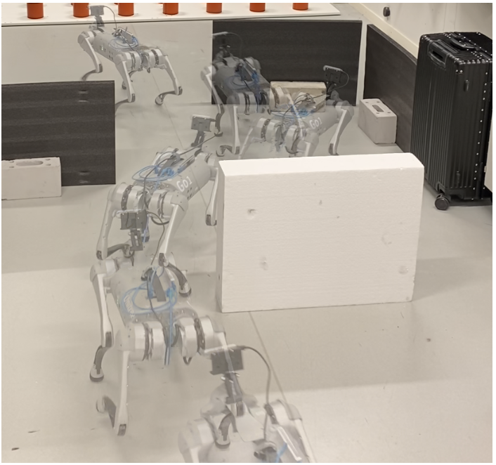
Figure 1: Visual CPG-RL navigation on Unitree Go1.

I-A Related Work

I-A1 Biology-Inspired Control

Central Pattern Generators are neural circuits located in the spinal cords of vertebrate animals that are capable of producing coordinated patterns of high-dimensional rhythmic output signals, with evidence from nature and experimentally validated on various robot hardware [1]. For quadrupedal robots, CPGs have been used as a tool to both replicate and understand locomotion from several points of view, including the role of sensory input, reflexes, and mechanical design inspired from biology [2, 3]. Quadruped robots have also shown evidence that gait generation and transitions can occur through simple force feedback, without any explicit coupling between oscillators [4, 5], and feedback from touch sensors can stop or accelerate transitions between swing/stance phases [6]. Other works have augmented CPGs with reflexes, Virtual Model Control, and push recovery for improved robustness [7, 8, 9]. Sensory feedback has not just been limited to proprioceptive information, for example a camera and gyroscope were used as feedback to a CPG to learn to walk over varying terrains in [10], and external sensory information allows responses to sudden obstacle appearances [11, 12].

I-A2 Model-Based Control

Conventional control approaches have shown impressive performance for real world robot locomotion [13, 14, 15, 16]. Such methods typically rely on solving online optimization problems (Model Predictive Control (MPC)) using simplified dynamics models, which require significant domain knowledge, and may not generalize to new environments not explicitly considered during development (i.e. uneven slippery terrain).

Vision in MPC: To improve the capabilities of “blind” policies, several recent works integrate filtered perception data as constraints during the optimization process [17, 18, 19, 20]. These works build an elevation map of the environment through one or more depth cameras [21, 22], and the resulting grid map [23] is postprocessed for smoothing, inpainting, or plane segmentation, depending on the application. More recent mapping software uses a GPU to accelerate this mapping process [24], and learning-based methods have also been shown to improve the accuracy of the map[25].

I-A3 Learning-Based Control

Deep reinforcement learning (DRL) has emerged as an attractive solution to train control policies that are robust to external disturbances and unseen environments in sim-to-real. Similarly to model-based control, recent works have shown successful results in training “blind” control policies, with only proprioceptive sensing being mapped to joint commands. For quadrupedal robots, such approaches have resulted in successful locomotion controllers on both flat [26, 27] and rough terrain [28, 29]. Blind policies have also shown state-of-the-art high-speed velocity tracking on the MIT mini-cheetah [30, 31]. Other works have shown the possibility of directly imitating animal motions [32], and the emergence of different gaits through minimizing energy consumption with DRL [33].

Vision in DRL: To improve on the reactive controllers trained only with proprioceptive sensing as input, recent works are integrating vision into the deep reinforcement learning framework. Similarly to the MPC approach, this has allowed for combining occupancy maps with proprioceptive sensing for navigation [34], obstacle avoidance with end-to-end training directly from pixels [35, 36], as well as more dynamic crossing of rough terrain through the use of sampling from height maps [37, 38]. Other works have decoupled footstep planning processes from the control policy, either each trained with DRL [39], or leveraging MPC to track the footstep plan [40]. Learning a state representation of the environment from depth images and sending high-level commands to a separately trained DRL control policy also allows navigating cluttered environments [41]. Additional works have shown gap crossing [42, 43, 44], also with full flight phases learned from pixels and leveraging MPC [45].

I-A4 Sim-to-Real Transfer

Directly mapping from proprioceptive sensing to joint space commands is a challenging problem, even for deep networks and millions of training samples. In addition to the complexity of carefully crafting reward functions to try to specify desired motions like foot swing height, there are difficulties with the sim-to-real transfer arising from unmodeled dynamics such as the actuators. There are several methods to improve the robustness of policies trained in simulation, such as domain randomization [46, 47] and dynamics randomization [48, 49, 50]. In addition to sufficient simulation environmental noise or accurate dynamics modeling, policy representation in terms of neural network architecture also plays an important role for the sim-to-real transfer. Previous works[51, 48, 52] have shown that a memory-enabled network (i.e. LSTM) has higher proficiency to deal with partially observable environments compared with purely feedforward networks (MLPs).

I-A5 Action Space and Phase in DRL

Action space choice has also been shown to have a large effect on sim-to-real performance and avoiding undesired local optima. Compared with the more common mapping to desired joint positions, recent works have shown the possibility of directly learning torques [53], desired task space foot positions [54, 55, 56], or encoding a time component (phase) into the framework, such as Policies Modulating Trajectory Generators (PMTG) for Minitaur [57] and ANYmal [29, 37]. Additionally, incorporating phase encodings facilitates learning different gaits [58], and can also be used together with MPC [59].

For biped robots, DRL has been used to directly learn the feedback terms of a CPG to tackle different slopes [60], or to update the parameters of a CPG-ZMP walk engine and output joint target residuals to adapt to commands and different terrains [61]. For quadrupeds, Shi et al. learn both the parameters of a foot trajectory generator as well as joint target residuals to locomote in a variety of environments including stairs and slopes [62]. In our previous work, we proposed CPG-RL [63], a framework for using deep reinforcement learning to directly learn the time-varying oscillator intrinsic amplitude and frequency for each oscillator which together forms a central pattern generator. We implemented the CPG network with one oscillator per limb, but without explicit couplings between oscillators, similarly to the work of Owaki et al. [5], and used only proprioceptive sensing.

I-B Contribution

In this paper, we extend our previous work to include terrain-awareness as feedback to the policy network, which enables navigation of cluttered terrain. We test different neural network architectures, specifically purely feedforward networks (MLPs) as well as memory-enabled networks (LSTMs), and find that the memory-enabled networks are more robust for the sim-to-real transfer. While the agent can learn implicit couplings between oscillators in the policy network through experience, we additionally test varying explicit couplings between oscillators in the dynamics equations. Such couplings between oscillators are known to exist in biological CPGs, but recent work has shown that they might be weaker than previously thought [5, 64], and that sensory feedback and descending modulation might play an important role in interoscillator synchronization. For the sim-to-real transfer, we find that explicit coupling improves policy robustness, especially when concatenating high-dimensional (and noisy) exteroceptive inputs with lower-dimensional proprioceptive sensing. In summary, this work addresses several questions: how to integrate vision and learning with CPGs, whether memory is useful for better sim-to-real performance, and whether gaits can best be generated by descending drives and/or by interoscillator couplings in the CPG.

The rest of this paper is organized as follows. Section II provides background details on deep reinforcement learning and Central Pattern Generators. Section III describes our design choices and integration of Central Pattern Generators and exteroceptive sensing into the deep reinforcement learning framework (Visual CPG-RL). Section IV shows results and analysis from learning our controller and a sim-to-real transfer for varying neural network architectures and specified interoscillator couplings, and a brief conclusion is given in Section V.

II Background

II-A Reinforcement Learning

In the reinforcement learning framework [65], an agent interacts with an environment modeled as a Markov Decision Process (MDP). An MDP is given by a 4-tuple $(\mathcal{S,A,P,R})$, where $\mathcal{S}$ is the set of states, $\mathcal{A}$ is the set of actions available to the agent, $\mathcal{P}:\mathcal{S}\times\mathcal{A}\times\mathcal{S}\rightarrow\mathbb{R}$ is the transition function, where $\mathcal{P}(s_{t+1}|s_{t},a_{t})$ gives the probability of being in state $s_{t}$, taking action $a_{t}$, and ending up in state $s_{t+1}$, and $\mathcal{R}:\mathcal{S}\times\mathcal{A}\times\mathcal{S}\rightarrow\mathbb{R}$ is the reward function, where $\mathcal{R}(s_{t},a_{t},s_{t+1})$ gives the expected reward for being in state $s_{t}$, taking action $a_{t}$, and ending in state $s_{t+1}$. The agent goal is to learn a policy $\pi$ that maximizes its expected return for a given task.

II-B Central Pattern Generators

While a number of neural oscillators have been proposed to implement CPG circuits, here we focus on the amplitude-controlled phase oscillators from [66] used to produce both swimming and walking behaviors on a salamander robot:

$$\ddot{r}_{i} =a\left(\frac{a}{4}\left(\mu_{i}-r_{i}\right)-\dot{r}_{i}\right)$$ (1)

$$\dot{\theta}_{i} =\omega_{i}+\sum_{j}r_{j}w_{ij}\sin(\theta_{j}-\theta_{i}-\phi_{ij})$$ (2)

where $r_{i}$ is the current amplitude of the oscillator, $\theta_{i}$ is the phase of the oscillator, $\mu_{i}$ and $\omega_{i}$ are the intrinsic amplitude and frequency, $a$ is a positive constant representing the convergence factor. Couplings between oscillators are defined by the weights $w_{ij}$ and phase biases $\phi_{ij}$.

For a quadruped robot with a single oscillator corresponding to each leg, a coupling matrix $\bm{\Phi}$ representing a trot gait can be defined as:

$$\bm{\Phi}=\begin{bmatrix}0&\pi&\pi&0\\ -\pi&0&0&-\pi\\ -\pi&0&0&-\pi\\ 0&\pi&\pi&0\end{bmatrix}$$ (3)

where the row/column order is Front Left (FL), Front Right (FR), Hind Left (HL), Hind Right (HR). With this matrix, and by properly tuning the parameters $a$, $w_{ij}$, $\mu_{i}$, $\omega_{i}$ (either by hand or through evolutionary algorithms such as CMA-ES [67]), it is possible to map the oscillator states to task space foot trajectories and track these at the joint level with inverse kinematics [6]. However, such a tuning results in a specific fixed open-loop gait which may not be robust to external disturbances.

III Learning Central Pattern Generators for Visual Navigation

In this section we describe our CPG-integrated deep reinforcement learning framework and design decisions for learning visual navigation controllers for quadruped robots. At a high level, the agent takes as input exteroceptive and proprioceptive sensing measurements and the current CPG state, and learns to modulate the CPG parameters for each leg with deep reinforcement learning to track velocity commands while avoiding collisions. This type of learning represents an approximation of motor learning in animals, namely how higher brain centers such as the motor cortex and the cerebellum learn to send modulation signals to CPG circuits in the spinal cord. The control diagram for our method is shown in Figure 2, and we discuss all components below.

III-A Action Space

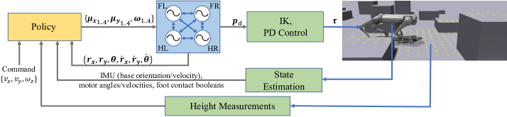
Figure 2: Control architecture for learning central pattern generators for quadruped navigation. Given an observation consisting of velocity commands, terrain height measurements, proprioceptive measurements, and the current CPG states, the policy network selects CPG parameters $\mu_{x}$, $\mu_{y}$ and $\omega$ for each leg $i$ (Front Left (FL), Front Right (FR), Hind Left (HL), Hind Right (HR)). The CPG states are mapped to desired foot positions $\bm{p}_{d}$, which are then converted to desired joint angles with inverse kinematics, and finally tracked with joint PD control to produce torques $\bm{\tau}$. The control policy selects actions at 100 Hz, and all other blocks operate at 1 kHz.

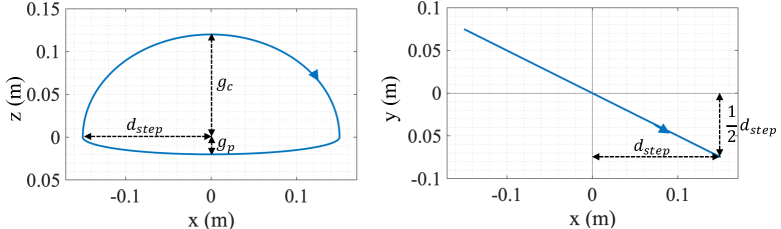
Figure 3: Mapping the CPG states to Cartesian foot positions. At left in the XZ-plane: ground clearance ($g_{c}$), ground penetration ($g_{p}$), max step length ($d_{step}$) are design parameters, whereas CPG states $r_{x}$ and $\theta$ control amplitude and phase. At right in the XY-plane: coordinating omnidirectional motion in the leg frame (arrow shows swing phase motion) with converged amplitude set points $\mu_{x}=2$, $\mu_{y}=1.75$, representing the full $d_{step}$ and $\frac{1}{2}d_{step}$, respectively.

We first consider the coupled oscillators in Equations 1 and 2 (one for each leg, or $i\in\{1,2,3,4\}$), whose output we will map to foot trajectories in Cartesian space similar to [6, 63]. In order to produce dynamic omnidirectional movements, we define a third state variable to represent amplitude in the $y$ direction within each leg frame (see Figure 3). The agent can then learn to coordinate both amplitudes for omnidirectional locomotion, and we update the coupling to reflect both $x$ and $y$ components. Thus, for each limb we define the following oscillator:

$$\ddot{r}_{x_{i}} =a_{x}\left(\frac{a_{x}}{4}\left(\mu_{x_{i}}-r_{x_{i}}\right)-\dot{r}_{x_{i}}\right)$$ (4)

$$\ddot{r}_{y_{i}} =a_{y}\left(\frac{a_{y}}{4}\left(\mu_{y_{i}}-r_{y_{i}}\right)-\dot{r}_{y_{i}}\right)$$ (5)

$$\dot{\theta}_{i} =\omega_{i}+\frac{1}{2}\sum_{j}(r_{x_{j}}+r_{y_{j}})w_{ij}\sin(\theta_{j}-\theta_{i}-\phi_{ij})$$ (6)

Our action space will directly modulate the intrinsic oscillator amplitudes and phases, by learning to modulate $\mu_{x_{i}}$, $\mu_{y_{i}}$, and $\omega_{i}$ for each leg. This allows the agent to adapt each of these states online in real-time depending on sensory inputs, compared with the more traditional CPG approach of optimizing for only a single set of fixed parameters. Thus, for the omnidirectional navigation task, our action space can be summarized as $\mathbf{a}=[\bm{\mu}_{x},\bm{\mu}_{y},\bm{\omega}]\in\mathbb{R}^{12}$. The agent selects these parameters at 100 Hz, and we use the following limits for each input during training: $\mu_{x},\mu_{y}\in[1,2]$, $\omega\in[0,4.5]$ Hz, and $a_{x}=a_{y}=50$.

To map from the oscillator states to joint commands, we first compute corresponding desired foot positions, and then calculate the desired joint positions with inverse kinematics. This is an approximation of the typical two layers found in mammalian CPGs, with one rhythm generating layer, and one pattern formation layer [68]. The desired foot position coordinates are given as follows:

$$x_{i,\text{foot}} =-d_{step}f(r_{x_{i}})\cos(\theta_{i})$$ (7)

$$y_{i,\text{foot}} =\phantom{-}d_{step}f(r_{y_{i}})\cos(\theta_{i})$$ (8)

$$z_{i,\text{foot}} =\begin{cases}-h+g_{c}\sin(\theta_{i})&\text{if }\sin(\theta_{i})>0\\ -h+g_{p}\sin(\theta_{i})&\text{otherwise}\end{cases}$$ (9)

where $d_{step}$ is the maximum step length, $h$ is the robot height, $g_{c}$ is the max ground clearance during swing, $g_{p}$ is the max ground penetration during stance, and $f(r)=2\frac{(r-\mu_{\text{min}})}{(\mu_{\text{max}}-\mu_{\text{min}})}-1$. In this mapping, since $r_{x_{i}}$ and $r_{y_{i}}$ each vary between $\mu_{\text{min}}=1$ and $\mu_{\text{max}}=2$, the foot can vary within $\pm d_{step}$ in both $x$ and $y$ directions in each leg frame.

A sample visualization of the foot trajectory for a set of these parameters is shown in Figure 3. These parameters make it possible to specify behaviors that are in general difficult to learn when directly learning joint commands. For example, specifying a foot swing height would usually necessitate keeping track of a history of states and exasperates the temporal credit assignment problem of reinforcement learning. With our framework, we randomly sample $h$, $g_{c}$, and $g_{p}$ during training (i.e. the agent has no explicit observation of these parameters) to learn continuous behavior, which then allows the user to specify both a robot height and swing foot ground clearance during deployment.

III-B Observation Space

Our observation space consists of velocity commands and measurements available with both exteroceptive and proprioceptive sensing. The exteroceptive measurements consist of querying a terrain height map at a $17\times 11$ grid spaced at intervals of 0.1 m around the robot base. In simulation, the ground truth terrain height data is known, and on hardware such a grid can be estimated, for example by using depth cameras to build an elevation map [21, 22], and then querying the resulting postprocessed grid map [23].

The proprioceptive sensing includes the body state (orientation, linear and angular velocities), joint state (positions, velocities), and foot contact booleans. The last action chosen by the policy network and CPG states $\{\bm{r}_{x},\bm{\dot{r}}_{x},\bm{r}_{y},\bm{\dot{r}}_{y},\bm{\theta},\bm{\dot{\theta}}\}$ are concatenated to the exteroceptive and proprioceptive measurements. Compared with the exteroceptive and proprioceptive sensing which are subject to measurement noise from onboard sensors, the CPG states are always known, and we believe this provides a source of stability to the method and eases the sim-to-real transfer.

III-C Reward Function

We design our reward function to track desired body velocity commands in the body frame $x$ and $y$ directions as well as a desired yaw rate $\omega_{b,z}^{*}$. We include terms to minimize other undesired body velocities as well as penalize the work (aiming at keeping the body stable and minimizing the energy consumption). More precisely, the reward function is a summation of the following terms:

• linear velocity tracking, body $x$ direction: $f(v_{b,x}^{*}-v_{b,x})$

• linear velocity tracking, body $y$ direction: $f(v_{b,y}^{*}-v_{b,y})$

• angular velocity tracking (body yaw rate): $f(\omega_{b,z}^{*}-\omega_{b,z})$

• linear velocity penalty in body $z$ direction: $-v_{b,z}^{2}$

• angular velocity penalty (body roll and pitch rates): $-||\bm{\omega}_{b,xy}||^{2}$

• work: $-|\bm{\tau}\cdot(\dot{\bm{q}}^{t}-\dot{\bm{q}}^{t-1})|$

where $(\cdot)^{*}$ represents a desired command, and $f(x):=\exp{(-\frac{||x||^{2}}{0.25})}$. These terms are weighted with $3dt$, $0.75dt$, $0.5dt$, $2dt$, $0.05dt$, $0.001dt$, where $dt=0.01$ is the control policy time step. Notably, as discussed in Section III-A, we do not need to put any additional terms on foot swing time or add other terms beyond those fully specifying base motion tracking. Due to the variable height terrain in the training environment, however, it is not possible to track all velocity commands at all times (i.e. if there are obstacles in the way). We more heavily weight the forward velocity reward term so the policy learns to prefer deviations to the other velocity commands/penalties (i.e. to turn if approaching an obstacle head-on).

TABLE I: PPO Hyperparameters.

Parameter	Value
Batch size	98304 (4096x24)
Mini-bach size	24576 (4096x6)
Number of epochs	5
Clip range	0.2
Entropy coefficient	0.01
Discount factor	0.99
GAE discount factor	0.95
Desired KL-divergence $kl^{*}$	0.01
Learning rate $\alpha$	adaptive

III-D Neural Network Architectures

We consider two different neural network architectures to map the concatenated proprioceptive and exteroceptive sensing observation to actions modulating the intrinsic oscillator amplitudes and phases. The first is a purely feedforward network, or multi-layer perceptron (MLP), consisting of three hidden layers of [512, 256, 128] hidden units per layer. The second architecture is a memory-enabled network, consisting of a Long Short-Term Memory (LSTM) layer of 512 hidden units, followed by two fully connected layers of [256, 128] hidden units. The memory-enabled network has a better biological parallel (i.e. humans do not need a full refresh of exteroceptive sensing at 100 Hz, and can walk blindly by remembering the terrain), and we also anticipate this will provide better robustness for the sim-to-real transfer in the event of noisy measurements and latency.

III-E Training Details

We use Isaac Gym [69, 38] with PhysX as our physics engine and training environment, and the Unitree Go1 quadruped [70]. This framework allows for high throughput, where we simulate 4096 Go1s in parallel on a single NVIDIA RTX 3090 GPU. We use PPO [71] to train the policy, and the relevant hyperparameters are listed in Table I. With this framework, similar to in [38, 63], we can learn control policies within minutes.

The maximum episode length is 20 seconds, and the environment resets for an agent if the base or a thigh comes in contact with the terrain (i.e. either a box or the ground). We employ a terrain curriculum starting from flat terrain, to random boxes of varying widths (0.4 to 2 m) and heights (0.1 to 1 m). With each reset, we sample new parameters $h$ and $g_{c}$ for the mapping from oscillator states to joint commands so the agent can learn to locomote at varying body heights and step heights. New velocity commands $\{v_{b,x}^{*},v_{b,y}^{*},\omega_{b,z}^{*}\}$ are sampled every 5 seconds. We also apply domain randomization on the physical mass properties and coefficient of friction, as summarized in Table II. An external push of up to 0.5 m/s is applied in a random direction to the base every 15 seconds. While no noise is added to the proprioceptive measurements, we add Gaussian noise to the exteroceptive measurements with a standard deviation of 0.1.

The control frequency of the policy is 100 Hz, and the torques computed from the desired joint positions are updated at 1 kHz. The equations for each of the oscillators (Equations 4-6) are thus also integrated at 1 kHz. During training we re-sample joint PD controller gains at each environment reset as described in Table II, but during deployment we use $K_{p}=100,\ K_{d}=2$.

TABLE II: Randomized parameters during training and their ranges.

Parameter	Lower Bound	Upper Bound	Units
$v_{b,x}^{*}$	-0.6	0.6	m/s
$v_{b,y}^{*}$	-0.4	0.4	m/s
$\omega_{b,z}^{*}$	-0.8	0.8	rad/s
Joint Gain $K_{p}$	55	100	-
Joint Gain $K_{d}$	0.7	2.5	-
Mass (each body link)	70	130	%
Added base mass	0	5	$kg$
Coefficient of friction	0.3	1	-

IV Experimental Results and Discussion

In this section we report results from learning visual navigation locomotion controllers with CPG-RL. Snapshots of some of our results are shown in Figure 1, and the reader is encouraged to watch the supplementary video for clear visualizations of the discussed experiments. We are specifically interested in the following questions:

• How does policy network architecture affect the sim-to-real transfer?

• What is the role of neural oscillator coupling in the sim-to-real transfer?

• How does the agent coordinate turning between different oscillators (amplitudes)?

IV-A Sim-to-Real Transfer

As in [17], we mount two Intel RealSense cameras (D435i and T265) on the Unitree Go1 quadruped [70]. The D435i is mounted forward-facing to provide point clouds to elevation mapping software [21, 22] to construct a map of the area surrounding the robot. The T265 provides high accuracy localization. To run the policy, we query this map at the same $17\times 11$ points around the robot as seen during training, and concatenate the proprioceptive sensing measurements as read by the Unitree sensors, along with the CPG states and previous actions.

IV-B Role of Policy Architecture and Interoscillator Coupling

We train policies with both neural network architectures (MLP and LSTM) described in Section III-D. For each architecture, we train separate policies for increasingly strong interoscillator coupling weights, namely $w_{i,j}=\{0,0.2,0.4,0.6,0.8,1.0\}$ in Equation 6, for a total of 6 MLP policies and 6 LSTM policies. We use the trot gait coupling matrix in Equation 3, since without coupling (i.e. $w_{i,j}=0$), all policies learn an approximate trot gait.

Interestingly, all policies achieve identical returns in simulation, regardless of architecture or oscillator coupling. This shows that even strong coupling does not have a negative effect on the ability of the policy to adapt to sensory feedback and coordinate omnidirectional locomotion.

IV-B1 Corridor Test

We first test all policies in a 1.7 m wide corridor and command a forward velocity of $v_{b,x}^{*}=0.35$ m/s for 10 seconds. This test is done to ensure successful sim-to-real transfers on (mostly) flat terrain, and mean results from 10 rollouts of each policy are shown for the MLP policies in Table III and LSTM policies in Table IV. All policies successfully locomote with 100% success rate with both MLP and LSTM architectures, with strong, weak, and no coupling. However, the LSTM policies have a lower Cost of Transport for all couplings. When comparing the mean amplitudes and frequencies, the LSTM policies locomote with a higher leg frequency but lower step length than the MLP policies. The LSTM policies also track the commanded velocity slightly more closely, and interestingly overshoot the command, compared with the MLP policies which are consistently slower.

IV-B2 Navigation Test

We next test all policies in a navigation environment which requires both left and right turns in order to avoid obstacles. We define a failure as the robot colliding with an obstacle or falling down. We again command a forward velocity of $v_{b,x}^{*}=0.35$ m/s for 10 seconds, and mean results from 10 rollouts of each policy are summarized in Tables V and VI. In order to avoid the obstacles, the agent is forced to violate at least one of the 0 velocity commands for $v_{b,y}^{*}$ and $\omega_{b,z}^{*}$. In these tests, for both the MLP and LSTM policies, we observe that coupling is beneficial for successful navigation of the terrain, where increasing the coupling leads to higher success rates for both architectures. The explicit coupling helps to reject noise and latency associated with the high-dimensional (relative to the proprioceptive) exteroceptive measurements. The LSTM policies also prove to be overall more robust than the MLP policies.

We also test commanding the agent to move forward directly into a wall. If started far enough away from the wall, or if there is an angle or non-symmetrical height map measurements, the agent is able to turn towards the wider angle and then move away from the wall. If initialized very close to the wall, the agent does not move, or steps very slowly in place.

IV-C CPG State Modulation for Omnidirectional Locomotion

We investigate how the agent modulates the CPG states to produce omnidirectional locomotion on flat terrain. Figure 4 shows the CPG states when commanded to move laterally in the body $y$ directions, $v_{b,y}^{*}=\pm 0.4$ m/s, and then turn in place in both directions, $\omega_{b,z}^{*}=\pm 0.7$ rad/s. The video shows that the gait is smooth and consistent for the entirety of the motion, at a much lower frequency than the default Go1 controller. The lateral motions show the amplitudes $y$ selecting the expected directions, and coordination can be seen between both $x$ and $y$ amplitudes for turning in place. An approximate trot gait can be observed throughout all commands. For turning left, for example, the hind right foot has the largest amplitude in the $x$ direction, which combined with the $y$ amplitude moving mostly right in the body frame, turns the system in the expected direction. The reverse is true for turning right, where the hind left foot has the largest amplitude in the $x$ direction, and combines with the $y$ amplitude now moving mostly left in the body frame.

TABLE III: Sim-to-real tracking performance of $v_{b,x}^{*}=0.35$ m/s in a wide corridor, with MLP policies trained with varying coupling weights ($w_{i,j}$ in Equation 6).

	MLP
Coupling Weight	0	0.2	0.4	0.6	0.8	1.0
COT	1.16	1.03	1.15	1.02	0.95	1.0
Mean Velocity (m/s)	0.31	0.29	0.32	0.30	0.33	0.34
Mean $\dot{\theta}$ (Hz)	1.08	0.97	1.14	0.97	0.91	1.17
Mean $r_{x}$	1.94	1.91	1.93	1.92	1.97	1.86
% Success	1	1	1	1	1	1

TABLE IV: Sim-to-real tracking performance of $v_{b,x}^{*}=0.35$ m/s in a wide corridor, with LSTM policies trained with varying coupling weights ($w_{i,j}$ in Equation 6)

	LSTM
Coupling Weight	0	0.2	0.4	0.6	0.8	1.0
COT	0.87	0.86	0.89	0.89	0.84	0.78
Mean Velocity (m/s)	0.38	0.39	0.39	0.38	0.39	0.41
Mean $\dot{\theta}$ (Hz)	2.04	2.20	2.12	2.11	2.05	2.0
Mean $r_{x}$	1.74	1.70	1.70	1.73	1.68	1.70
% Success	1	1	1	1	1	1

TABLE V: Sim-to-real tracking performance of $v_{b,x}^{*}=0.35$ m/s in a test navigation environment involving both left and right turns, with MLP policies trained with varying coupling weights ($w_{i,j}$ in Equation 6).

	MLP
Coupling Weight	0	0.2	0.4	0.6	0.8	1.0
COT	1.32	1.35	1.13	1.10	1.20	1.23
Mean Velocity (m/s)	0.29	0.26	0.31	0.34	0.32	0.31
Mean $\dot{\theta}$ (Hz)	1.32	1.35	1.13	1.10	1.20	1.23
Mean $r_{x}$	1.93	1.91	1.79	1.87	1.94	1.88
% Success	0.6	0.6	0.8	1.0	0.9	0.9

TABLE VI: Sim-to-real tracking performance of $v_{b,x}^{*}=0.35$ m/s in a test navigation environment involving both left and right turns, with LSTM policies trained with varying coupling weights ($w_{i,j}$ in Equation 6).

	LSTM
Coupling Weight	0	0.2	0.4	0.6	0.8	1.0
COT	1.01	0.81	0.81	0.94	0.80	0.79
Mean Velocity (m/s)	0.38	0.40	0.40	0.42	0.39	0.40
Mean $\dot{\theta}$ (Hz)	2.05	2.23	2.07	2.02	1.98	1.99
Mean $r_{x}$	1.73	1.68	1.69	1.73	1.69	1.70
% Success	0.8	0.9	1.0	0.9	1.0	1.0

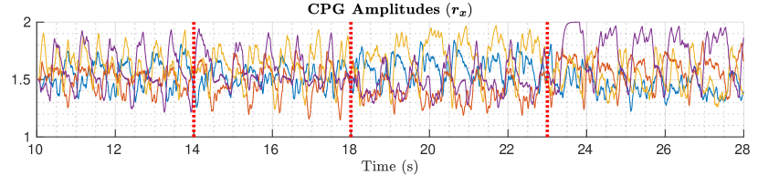
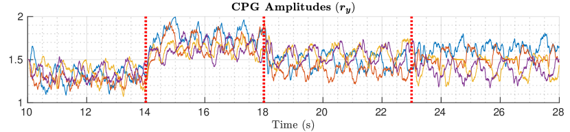
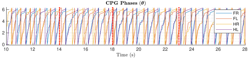
Figure 4: CPG states during omnidirectional commands: $v_{b,y}^{*}=0.4$ m/s from 10-14 s, $v_{b,y}^{*}=-0.4$ m/s from 14-18 s, $\omega_{b,z}^{*}=0.7$ rad/s from 18-23 s, and $\omega_{b,z}^{*}=-0.7$ rad/s from 23-28 s. The $y$ amplitudes $r_{y}$ produce locomotion for the system for the lateral commands. For turning in place, we observe coordination between both $x$ and $y$ amplitudes.

V Conclusion

In this work we have presented Visual CPG-RL, a framework for learning quadruped navigation by integrating central pattern generators and exteroceptive sensing into the deep reinforcement learning framework. The agent learns to modulate the intrinsic oscillator amplitudes and frequencies to coordinate rhythmic behavior among limbs to track omnidirectional velocity commands, while also learning to deviate from the commands in order to avoid collisions with obstacles. Our results show that memory-enabled networks (i.e. LSTMs) provide higher robustness than feedforward networks (MLPs) for navigation tasks which may have high-dimensional inputs, noise, and latency concerns. We also showed that explicit coupling in the dynamics equations is beneficial for the sim-to-real navigation task, and does not impair the agent’s ability to learn robust, adaptive, and efficient policies. Future work will focus on adding additional states to the CPG to account for rough terrain, as well as compare with joint-space CPGs, towards a better understanding of the biological parallels in learning legged locomotion.

References

- [1] A. J. Ijspeert, “Central pattern generators for locomotion control in animals and robots: A review,” Neural Networks, vol. 21, no. 4, pp. 642–653, 2008, robotics and Neuroscience.
- [2] Y. Fukuoka, H. Kimura, and A. H. Cohen, “Adaptive dynamic walking of a quadruped robot on irregular terrain based on biological concepts,” The International Journal of Robotics Research, vol. 22, no. 3-4, pp. 187–202, 2003.
- [3] A. Spröwitz, A. Tuleu, M. Vespignani, M. Ajallooeian, E. Badri, and A. J. Ijspeert, “Towards dynamic trot gait locomotion: Design, control, and experiments with cheetah-cub, a compliant quadruped robot,” The International Journal of Robotics Research, vol. 32, no. 8, pp. 932–950, 2013.
- [4] D. Owaki, T. Kano, K. Nagasawa, A. Tero, and A. Ishiguro, “Simple robot suggests physical interlimb communication is essential for quadruped walking,” Journal of The Royal Society Interface, vol. 10, no. 78, p. 20120669, 2013.
- [5] D. Owaki and A. Ishiguro, “A quadruped robot exhibiting spontaneous gait transitions from walking to trotting to galloping,” Scientific reports, vol. 7, no. 1, pp. 1–10, 2017.
- [6] L. Righetti and A. J. Ijspeert, “Pattern generators with sensory feedback for the control of quadruped locomotion,” in IEEE International Conference on Robotics and Automation, 2008, pp. 819–824.
- [7] M. Ajallooeian, S. Pouya, A. Sproewitz, and A. J. Ijspeert, “Central pattern generators augmented with virtual model control for quadruped rough terrain locomotion,” in 2013 IEEE International Conference on Robotics and Automation, 2013, pp. 3321–3328.
- [8] M. Ajallooeian, S. Gay, A. Tuleu, A. Spröwitz, and A. J. Ijspeert, “Modular control of limit cycle locomotion over unperceived rough terrain,” in 2013 IEEE/RSJ International Conference on Intelligent Robots and Systems, 2013, pp. 3390–3397.
- [9] V. Barasuol, J. Buchli, C. Semini, M. Frigerio, E. R. De Pieri, and D. G. Caldwell, “A reactive controller framework for quadrupedal locomotion on challenging terrain,” in 2013 IEEE International Conference on Robotics and Automation. IEEE, 2013, pp. 2554–2561.
- [10] S. Gay, J. Santos-Victor, and A. Ijspeert, “Learning robot gait stability using neural networks as sensory feedback function for central pattern generators,” in 2013 IEEE/RSJ International Conference on Intelligent Robots and Systems, 2013, pp. 194–201.
- [11] A. A. Saputra, N. Takesue, K. Wada, A. J. Ijspeert, and N. Kubota, “Aquro: A cat-like adaptive quadruped robot with novel bio-inspired capabilities,” Frontiers in Robotics and AI, vol. 8, p. 562524, 2021.
- [12] A. A. Saputra, J. Botzheim, A. J. Ijspeert, and N. Kubota, “Combining reflexes and external sensory information in a neuromusculoskeletal model to control a quadruped robot,” IEEE Transactions on Cybernetics, 2021.
- [13] J. Di Carlo, P. M. Wensing, B. Katz, G. Bledt, and S. Kim, “Dynamic locomotion in the mit cheetah 3 through convex model-predictive control,” in 2018 IEEE/RSJ International Conference on Intelligent Robots and Systems (IROS), 2018, pp. 1–9.
- [14] D. Kim, J. Di Carlo, B. Katz, G. Bledt, and S. Kim, “Highly dynamic quadruped locomotion via whole-body impulse control and model predictive control,” arXiv preprint arXiv:1909.06586, 2019.
- [15] M. Sombolestan, Y. Chen, and Q. Nguyen, “Adaptive force-based control for legged robots,” in 2021 IEEE/RSJ International Conference on Intelligent Robots and Systems (IROS), 2021, pp. 7440–7447.
- [16] C. D. Bellicoso, F. Jenelten, C. Gehring, and M. Hutter, “Dynamic locomotion through online nonlinear motion optimization for quadrupedal robots,” IEEE Robotics and Automation Letters, vol. 3, no. 3, pp. 2261–2268, 2018.
- [17] D. Kim, D. Carballo, J. Di Carlo, B. Katz, G. Bledt, B. Lim, and S. Kim, “Vision aided dynamic exploration of unstructured terrain with a small-scale quadruped robot,” in 2020 IEEE International Conference on Robotics and Automation (ICRA). IEEE, 2020, pp. 2464–2470.
- [18] R. Grandia, F. Jenelten, S. Yang, F. Farshidian, and M. Hutter, “Perceptive locomotion through nonlinear model predictive control,” arXiv preprint arXiv:2208.08373, 2022.
- [19] F. Jenelten, R. Grandia, F. Farshidian, and M. Hutter, “Tamols: Terrain-aware motion optimization for legged systems,” IEEE Transactions on Robotics, 2022.
- [20] A. Agrawal, S. Chen, A. Rai, and K. Sreenath, “Vision-aided dynamic quadrupedal locomotion on discrete terrain using motion libraries,” in 2022 International Conference on Robotics and Automation (ICRA). IEEE, 2022, pp. 4708–4714.
- [21] P. Fankhauser, M. Bloesch, and M. Hutter, “Probabilistic terrain mapping for mobile robots with uncertain localization,” IEEE Robotics and Automation Letters (RA-L), vol. 3, no. 4, pp. 3019–3026, 2018.
- [22] P. Fankhauser, M. Bloesch, C. Gehring, M. Hutter, and R. Siegwart, “Robot-centric elevation mapping with uncertainty estimates,” in International Conference on Climbing and Walking Robots (CLAWAR), 2014.
- [23] P. Fankhauser and M. Hutter, “A Universal Grid Map Library: Implementation and Use Case for Rough Terrain Navigation,” in Robot Operating System (ROS) – The Complete Reference (Volume 1), A. Koubaa, Ed. Springer, 2016, ch. 5.
- [24] T. Miki, L. Wellhausen, R. Grandia, F. Jenelten, T. Homberger, and M. Hutter, “Elevation mapping for locomotion and navigation using gpu,” arXiv preprint arXiv:2204.12876, 2022.
- [25] D. Hoeller, N. Rudin, C. Choy, A. Anandkumar, and M. Hutter, “Neural scene representation for locomotion on structured terrain,” IEEE Robotics and Automation Letters, vol. 7, no. 4, pp. 8667–8674, 2022.
- [26] J. Tan, T. Zhang, E. Coumans, A. Iscen, Y. Bai, D. Hafner, S. Bohez, and V. Vanhoucke, “Sim-to-real: Learning agile locomotion for quadruped robots.” in Robotics: Science and Systems, 2018.
- [27] J. Hwangbo, J. Lee, A. Dosovitskiy, D. Bellicoso, V. Tsounis, V. Koltun, and M. Hutter, “Learning agile and dynamic motor skills for legged robots,” Science Robotics, vol. 4, no. 26, 2019.
- [28] A. Kumar, Z. Fu, D. Pathak, and J. Malik, “Rma: Rapid motor adaptation for legged robots,” arXiv preprint arXiv:2107.04034, 2021.
- [29] J. Lee, J. Hwangbo, L. Wellhausen, V. Koltun, and M. Hutter, “Learning quadrupedal locomotion over challenging terrain,” Science Robotics, vol. 5, no. 47, 2020.
- [30] G. Ji, J. Mun, H. Kim, and J. Hwangbo, “Concurrent training of a control policy and a state estimator for dynamic and robust legged locomotion,” IEEE Robotics and Automation Letters, vol. 7, no. 2, pp. 4630–4637, 2022.
- [31] G. B. Margolis, G. Yang, K. Paigwar, T. Chen, and P. Agrawal, “Rapid locomotion via reinforcement learning,” arXiv preprint arXiv:2205.02824, 2022.
- [32] X. B. Peng, E. Coumans, T. Zhang, T.-W. Lee, J. Tan, and S. Levine, “Learning agile robotic locomotion skills by imitating animals,” 2020.
- [33] Z. Fu, A. Kumar, J. Malik, and D. Pathak, “Minimizing energy consumption leads to the emergence of gaits in legged robots,” in 5th Annual Conference on Robot Learning, 2021.
- [34] Z. Fu, A. Kumar, A. Agarwal, H. Qi, J. Malik, and D. Pathak, “Coupling vision and proprioception for navigation of legged robots,” in Proceedings of the IEEE/CVF Conference on Computer Vision and Pattern Recognition, 2022, pp. 17 273–17 283.
- [35] R. Yang, M. Zhang, N. Hansen, H. Xu, and X. Wang, “Learning vision-guided quadrupedal locomotion end-to-end with cross-modal transformers,” arXiv preprint arXiv:2107.03996, 2021.
- [36] C. S. Imai, M. Zhang, Y. Zhang, M. Kierebinski, R. Yang, Y. Qin, and X. Wang, “Vision-guided quadrupedal locomotion in the wild with multi-modal delay randomization,” arXiv preprint arXiv:2109.14549, 2021.
- [37] T. Miki, J. Lee, J. Hwangbo, L. Wellhausen, V. Koltun, and M. Hutter, “Learning robust perceptive locomotion for quadrupedal robots in the wild,” Science Robotics, 2022.
- [38] N. Rudin, D. Hoeller, P. Reist, and M. Hutter, “Learning to walk in minutes using massively parallel deep reinforcement learning,” in 5th Annual Conference on Robot Learning, 2021.
- [39] V. Tsounis, M. Alge, J. Lee, F. Farshidian, and M. Hutter, “Deepgait: Planning and control of quadrupedal gaits using deep reinforcement learning,” IEEE Robotics and Automation Letters, vol. 5, no. 2, pp. 3699–3706, 2020.
- [40] S. Gangapurwala, M. Geisert, R. Orsolino, M. Fallon, and I. Havoutis, “Rloc: Terrain-aware legged locomotion using reinforcement learning and optimal control,” IEEE Transactions on Robotics, 2022.
- [41] D. Hoeller, L. Wellhausen, F. Farshidian, and M. Hutter, “Learning a state representation and navigation in cluttered and dynamic environments,” IEEE Robotics and Automation Letters, vol. 6, no. 3, pp. 5081–5088, 2021.
- [42] W. Yu, D. Jain, A. Escontrela, A. Iscen, P. Xu, E. Coumans, S. Ha, J. Tan, and T. Zhang, “Visual-locomotion: Learning to walk on complex terrains with vision,” in 5th Annual Conference on Robot Learning, 2021.
- [43] K.-H. Lee, O. Nachum, T. Zhang, S. Guadarrama, J. Tan, and W. Yu, “Pi-ars: Accelerating evolution-learned visual-locomotion with predictive information representations,” arXiv preprint arXiv:2207.13224, 2022.
- [44] Z. Xie, X. Da, B. Babich, A. Garg, and M. van de Panne, “Glide: Generalizable quadrupedal locomotion in diverse environments with a centroidal model,” arXiv preprint arXiv:2104.09771, 2021.
- [45] G. B. Margolis, T. Chen, K. Paigwar, X. Fu, D. Kim, S. bae Kim, and P. Agrawal, “Learning to jump from pixels,” in 5th Annual Conference on Robot Learning, 2021.
- [46] J. Tobin, R. Fong, A. Ray, J. Schneider, W. Zaremba, and P. Abbeel, “Domain randomization for transferring deep neural networks from simulation to the real world,” in 2017 IEEE/RSJ international conference on intelligent robots and systems (IROS). IEEE, 2017, pp. 23–30.
- [47] I. Exarchos, Y. Jiang, W. Yu, and C. K. Liu, “Policy transfer via kinematic domain randomization and adaptation,” in 2021 IEEE International Conference on Robotics and Automation (ICRA). IEEE, 2021, pp. 45–51.
- [48] X. B. Peng, M. Andrychowicz, W. Zaremba, and P. Abbeel, “Sim-to-real transfer of robotic control with dynamics randomization,” in 2018 IEEE international conference on robotics and automation (ICRA). IEEE, 2018, pp. 3803–3810.
- [49] I. Mordatch, K. Lowrey, and E. Todorov, “Ensemble-cio: Full-body dynamic motion planning that transfers to physical humanoids,” in 2015 IEEE/RSJ International Conference on Intelligent Robots and Systems (IROS). IEEE, 2015, pp. 5307–5314.
- [50] Z. Xie, X. Da, M. van de Panne, B. Babich, and A. Garg, “Dynamics randomization revisited: A case study for quadrupedal locomotion,” in 2021 IEEE International Conference on Robotics and Automation (ICRA). IEEE, 2021, pp. 4955–4961.
- [51] J. Siekmann, K. Green, J. Warila, A. Fern, and J. Hurst, “Blind bipedal stair traversal via sim-to-real reinforcement learning,” arXiv preprint arXiv:2105.08328, 2021.
- [52] J. Siekmann, S. Valluri, J. Dao, F. Bermillo, H. Duan, A. Fern, and J. Hurst, “Learning Memory-Based Control for Human-Scale Bipedal Locomotion,” in Robotics: Science and Systems, 2020.
- [53] S. Chen, B. Zhang, M. W. Mueller, A. Rai, and K. Sreenath, “Learning torque control for quadrupedal locomotion,” arXiv preprint arXiv:2203.05194, 2022.
- [54] G. Bellegarda and K. Byl, “Training in task space to speed up and guide reinforcement learning,” in 2019 IEEE/RSJ International Conference on Intelligent Robots and Systems, 2019, pp. 2693–2699.
- [55] G. Bellegarda and Q. Nguyen, “Robust quadruped jumping via deep reinforcement learning,” arXiv preprint arXiv:2011.07089, 2020.
- [56] G. Bellegarda and Q. Nguyen, “Robust high-speed running for quadruped robots via deep reinforcement learning,” arXiv preprint arXiv:2103.06484, 2021.
- [57] A. Iscen, K. Caluwaerts, J. Tan, T. Zhang, E. Coumans, V. Sindhwani, and V. Vanhoucke, “Policies modulating trajectory generators,” in Conference on Robot Learning. PMLR, 2018, pp. 916–926.
- [58] Y. Shao, Y. Jin, X. Liu, W. He, H. Wang, and W. Yang, “Learning free gait transition for quadruped robots via phase-guided controller,” arXiv preprint arXiv:2201.00206, 2022.
- [59] Y. Yang, T. Zhang, E. Coumans, J. Tan, and B. Boots, “Fast and efficient locomotion via learned gait transitions,” in 5th Annual Conference on Robot Learning, 2021.
- [60] C. Li, R. Lowe, and T. Ziemke, “Humanoids learning to walk: A natural cpg-actor-critic architecture,” Frontiers in Neurorobotics, vol. 7, p. 5, 2013.
- [61] M. Kasaei, M. Abreu, N. Lau, A. Pereira, and L. P. Reis, “A cpg-based agile and versatile locomotion framework using proximal symmetry loss,” arXiv preprint arXiv:2103.00928, 2021.
- [62] H. Shi, B. Zhou, H. Zeng, F. Wang, Y. Dong, J. Li, K. Wang, H. Tian, and M. Q.-H. Meng, “Reinforcement learning with evolutionary trajectory generator: A general approach for quadrupedal locomotion,” arXiv preprint arXiv:2109.06409, 2021.
- [63] G. Bellegarda and A. Ijspeert, “CPG-RL: Learning central pattern generators for quadruped locomotion,” IEEE Robotics and Automation Letters, vol. 7, no. 4, pp. 12 547–12 554, 2022.
- [64] R. Thandiackal, K. Melo, L. Paez, J. Herault, T. Kano, K. Akiyama, F. Boyer, D. Ryczko, A. Ishiguro, and A. J. Ijspeert, “Emergence of robust self-organized undulatory swimming based on local hydrodynamic force sensing,” Science Robotics, vol. 6, no. 57, 2021.
- [65] R. S. Sutton and A. G. Barto, Reinforcement learning - an introduction, ser. Adaptive computation and machine learning. MIT Press, 1998.
- [66] A. J. Ijspeert, A. Crespi, D. Ryczko, and J.-M. Cabelguen, “From swimming to walking with a salamander robot driven by a spinal cord model,” Science, vol. 315, no. 5817, pp. 1416–1420, 2007.
- [67] N. Hansen, “The cma evolution strategy: A tutorial,” arXiv preprint arXiv:1604.00772, 2016.
- [68] D. A. McCrea and I. A. Rybak, “Organization of mammalian locomotor rhythm and pattern generation,” Brain research reviews, vol. 57, no. 1, pp. 134–146, 2008.
- [69] V. Makoviychuk, L. Wawrzyniak, Y. Guo, M. Lu, K. Storey, M. Macklin, D. Hoeller, N. Rudin, A. Allshire, A. Handa et al., “Isaac gym: High performance gpu-based physics simulation for robot learning,” arXiv preprint arXiv:2108.10470, 2021.
- [70] Unitree Robotics. Go1. https://www.unitree.com/products/go1/.
- [71] J. Schulman, F. Wolski, P. Dhariwal, A. Radford, and O. Klimov, “Proximal policy optimization algorithms,” CoRR, vol. abs/1707.06347, 2017.