AttEntropy: Segmenting Unknown Objects in Complex Scenes using the Spatial Attention Entropy of Semantic Segmentation Transformers

Abstract

Vision transformers have emerged as powerful tools for many computer vision tasks. It has been shown that their features and class tokens can be used for salient object segmentation. However, the properties of segmentation transformers remain largely unstudied. In this work we conduct an in-depth study of the spatial attentions of different backbone layers of semantic segmentation transformers and uncover interesting properties.

The spatial attentions of a patch intersecting with an object tend to concentrate within the object, whereas the attentions of larger, more uniform image areas rather follow a diffusive behavior. In other words, vision transformers trained to segment a fixed set of object classes generalize to objects well beyond this set. We exploit this by extracting heatmaps that can be used to segment unknown objects within diverse backgrounds, such as obstacles in traffic scenes.

Our method is training-free and its computational overhead negligible. We use off-the-shelf transformers trained for street-scene segmentation to process other scene types.

Figure 1: Entropy heatmaps. For each image patch, we compute the Shannon entropy of outgoing attentions. The two images in the right column depict the spatial attention at two different image locations. The bottom left images shows the Shannon entropy. Small objects receive concentrated attention and thus low corresponding entropy. An interactive tool for attention visualization is included in the supplementary material.

1 Introduction

Vision transformers have become increasingly popular for several computer vision tasks, including semantic image segmentation where they now achieve state-of-the-art performance [43, 41, 16]. However, as their CNN-based counterparts [42, 10, 36], these models are trained to segment a pre-defined set of object categories. As such, when faced with an image containing a semantically-unknown object, they will assign it to either one of the known classes or the background one. In this work, we show that, in fact, semantic segmentation transformers inherently contain valuable information to segment unknown objects.

For image recognition purposes, it has been shown that classification transformers could be employed to segment foreground objects [1, 6, 39]. This, however, was only demonstrated for simple scenes depicting one main object, and by exploiting either latent features at the end of the transformer backbone [1] or the final class tokens [6, 39]. Here, we go one step further and study the behavior of vision transformers in complex scenes containing multiple objects, such as those depicted by Fig. 1. In particular, we show that the intermediate attention maps of a semantic segmentation transformer trained on known object classes can be exploited to segment unknown ones.

In other words, we perform the first study of the spatial attention maps extracted in vision transformers by comparing image patches. Our analysis of different vision transformers reveals that

• While each local patch is connected to all the others, spatial attention tends to focus on semantically-similar neighboring image regions. As illustrated in Fig. 1, the attention diffuses farther from the patch in large uniform regions.

• For objects of small to moderate size, the attention concentrates within the object, independently of whether it belongs to a known or unknown category.

To put these observations to practical use, we exploit Shannon entropy and extract heatmaps from spatial attention, which, after minimal post-processing, can be directly used to segment unknown objects by simple thresholding.

We demonstrate the effectiveness of our method quantitatively on the task of road obstacle segmentation for which suitable benchmarks are available [7, 34]. We further show the generality of our analysis by demonstrating qualitatively that a semantic segmentation transformer trained on street scenes can be applied without any further training to accurately segment unknown objects in water scenes.

Our contributions can be summarized as follows:

• We provide an in-depth study of the different attention layers of vision transformers trained for semantic segmentation.

• We extract the entropy of spatial attentions and show that it can be used for unknown object segmentation.

• We demonstrate the generality of our approach using two semantic segmentation transformers [43, 41].

Our experiments on both on road scenes and water scenes evidence our method’s independence of the underlying task. On road obstacle segmentation benchmarks, we beat the state-of-the-art untrained methods and approach the accuracy of methods that are have been trained specifically for this task. We will make our code, including our analysis tool, publicly available.

2 Related Work

Segmentation / Localization and Attention.

A moderate number of works use features or attention from transformer backbones for object detection [22, 37] or semantic segmentation [1, 23, 6, 39]. In particular, the works of [1, 23] use transformer features to segment objects. However, they do not focus on segmenting unseen objects, but rather on segmenting seen ones under weak supervision [1] or even no supervision [23].

Probably closest to our work are the works of [6, 39] that are based on transformers learned via self-supervision. They can be considered to some extent as operating in an open world setting as the transformers have been trained on ImageNet [14] and then applied to other datasets. The work of [39] utilizes the transformer from [6]. It then constructs a graph based on the last layer features, and performs segmentation via a graph cut algorithm. In contrast to our work, the attention itself is not utilized in [39]. The work of [6] performs segmentation based on the final layer class tokens from the transformer attention. In contrast to both works [39, 6], we consider the attention between image patches across different layers, study their properties and use an information theoretic approach to segment potentially unknown obstacles in street scenes. Furthermore, both works rely on transformers trained in a self-supervised fashion with image classification as a target task. By contrast, our work constitutes the first study showing that a semantic segmentation transformer trained in a supervised fashion on known classes inherently learns to segment unknown objects.

Obstacle Detection. As obstacle detection is our main benchmark, we briefly review the existing works in that field. Most of the road obstacle segmentation methods (or the closely related road anomaly segmentation ones) can be grouped into two predominant approaches; 1) pasting synthetically generated obstacles or obstacles from other datasets into an image and then learning to detect them [2, 20, 21, 30], and 2) performing in-painting (sometimes conditioned on predicted segmentation masks) and then assessing the deviation from the input [15, 31, 40, 13, 29]. Besides these approaches, proxy datasets for anomalies or collections of prediction errors have also been used to learn uncertainties on anomalies and obstacles [8, 33, 5].

Methods that do not require any learning on the notion of road obstacle or road anomaly (while still being specifically designed for those tasks) are rare. Most of them are based on uncertainty estimation and rather serve as baselines. They have been transferred from image classification without any further task-specific development, e.g., Monte-Carlo dropout or maximum softmax probability [18, 24].

In contrast to these works, we propose a method to segment obstacles from the attention maps computed inside the semantic segmentation network with a negligible computation overhead.

3 From Attention to Segmentation

We first remind the reader of the attention mechanism that is at the heart of all transformer architectures. We then show how to use the attention matrices to create entropy heatmaps that highlight small size objects. Finally, we discuss our implementation.

3.1 Attention Mechanism in Visual Transformers

The Visual Transformer (ViT) [16] is one of the first successful applications of the transformer self-attention mechanism to image inputs. With enough training data, it can be more powerful than a traditional convolutional network for image classification. Furthermore, it serves as a backbone feature extractor for Segmentation Transformer (SETR) [43], providing improvement in semantic segmentation of road scenes over comparable convolutional backbones. We base the following description on the widely popular ViT architecture, but will show at the end of the section how it can be implemented for the differently structured Segformer [41].

ViT first decomposes the image in a checkerboard fashion into $N\times N$ image patches, each of size $16\times 16$ pixels, calculates their initial encodings and adds a learned spatial embedding, which will allow nearby patches to attend strongly to each other. The patches serve as tokens in the transformer: the attention mechanism connects each patch to all others.

The backbone consists of $L$ multi-head self-attention ($\mathit{MSA}$) blocks. Each attention block, or layer, $l$ receives as input a triplet $(\mbox{query}\;Q,\;\mbox{key}\;K,\;\mbox{value}\;V)$ computed itself from an input $Z^{l-1}\in\mathbb{R}^{N^{2}\times C}$, where $C$ denotes the number of feature channels. The triplet is computed from $Z^{l-1}$ as

$$\mathit{Q}=Z^{l-1}W_{Q},\leavevmode\nobreak\ \leavevmode\nobreak\ \mathit{K}=Z^{l-1}W_{K},\leavevmode\nobreak\ \leavevmode\nobreak\ \mathit{V}=Z^{l-1}W_{V},$$ (1)

where $W_{Q},W_{K},W_{V}\in\mathbb{R}^{C\times d}$ are learnable weight matrices and $d\in\mathbb{N}$ a parameter which we specify below. The attention $A^{l}$, which is the matrix that concerns us most in this paper, is taken to be

$$A^{l}(Z^{l-1})=\mathrm{softmax}(Q\cdot K^{T}/\sqrt{d})\,.$$ (2)

The softmax acts row-wise, so that the outgoing attention of each token sums up to 1. In the multi-head scenario, the attention is in fact computed multiple times. This yields $m$ independent attention matrices $\mathit{A}^{l}_{i}$, $i=1,\ldots,m$. While we will later focus on the attention matrices, for the sake of completeness, we derive the corresponding self-attention $\mathit{SA}$. It is expressed as

$$\mathit{SA}^{l}(Z^{l-1})=A^{l}(Z^{l-1})\cdot\mathit{V}\,.$$ (3)

Again, accounting for the multiple heads, this results in $m$ independent self-attention matrices $\mathit{SA}^{l}_{i}$, $i=1,\ldots,m$, that are concatenated

$$\mathit{SA}^{l}_{1:m}(Z^{l-1})=[\mathit{SA}^{l}_{1}(Z^{l-1}),\ldots,\mathit{SA}^{l}_{m}(Z^{l-1})]$$ (4)

and then multiplied with another weight matrix $W_{O}\in\mathbb{R}^{md\times C}$. Combined with a skip connection, this gives

$$\mathit{MSA}^{l}(Z^{l-1})=\mathit{SA}^{l}_{1:m}(Z^{l-1})+\mathit{SA}^{l}_{1:m}(Z^{l-1})W_{O}\,,$$ (5)

and, as in [43], we choose $d=C/m$. Finally, $\mathit{MSA}^{l}(Z^{l-1})$ is again input to a multilayer perceptron ($\mathit{MLP}$) block with a skip connection. This yields

$$Z^{l}=\mathit{MSA}^{l}(Z^{l-1})+\mathit{MLP}(\mathit{MSA}^{l}(Z^{l-1}))\in\mathbb{R}^{N^{2}\times C}\,.$$ (6)

Properties of the Attention Tensors. As described above, ViT [16] computes attention matrices $A^{l}_{i}(Z^{l-1})$ for layers $l=1,\ldots,L$ and for multiple heads $i=1,\ldots,m$. Due to the softmax activation and the decomposition of the image into patches, these attentions can be viewed as containing probability distributions over the $N\times N$ image patches plus the extra class-token, which we discard due to it lacking a geometric interpretation. For all $j,j^{\prime}\in\{1,\ldots,N^{2}\}$ in layer $l$, the element $A^{l}_{i}(Z^{l-1})_{j,j^{\prime}}$ of the attention matrix reflects how much attention patch $j$ pays to patch $j^{\prime}$.

These elements can therefore be visualized as heatmaps over the $N\times N$ image patches, as shown in Fig. 1, where we visualize the attention averaged over the multiple heads

$$\bar{A}^{l}(Z^{l-1})_{j,j^{\prime}}=\frac{1}{m}\sum_{i=1}^{m}A^{l}_{i}(Z^{l-1})_{j,j^{\prime}}\,.$$ (7)

Attention is driven by visual similarity and, thanks to the spatial embedding, proximity. We observe that attention originating from visually distinct moderately sized objects remains concentrated sharply within patches $j$ overlapping to a greater extent with that object. By contrast, for larger areas of visual coherence, such as the road, the attention is more dispersed over the entire region.

3.2 From Attention to Entropy Heatmaps

We quantify this behavior by estimating the Spatial Shannon Entropy

$$E^{l}(Z^{l-1})_{j}=-\sum_{j^{\prime}=1}^{N^{2}}\bar{A}^{l}(Z^{l-1})_{j,j^{\prime}}\cdot\log(\bar{A^{l}}(Z^{l-1})_{j,j^{\prime}})$$ (8)

for each image patch $j=1,\ldots,N^{2}$. The overall spatial entropy $\mathbf{E}^{l}=[E^{l}(Z^{l-1})_{j}]_{j\in\{1,\ldots,N^{2}\}}$ for layer $l$ can be viewed as an aggregated heatmap for layer $l$ that can be used to segment objects of limited size, as discussed below.

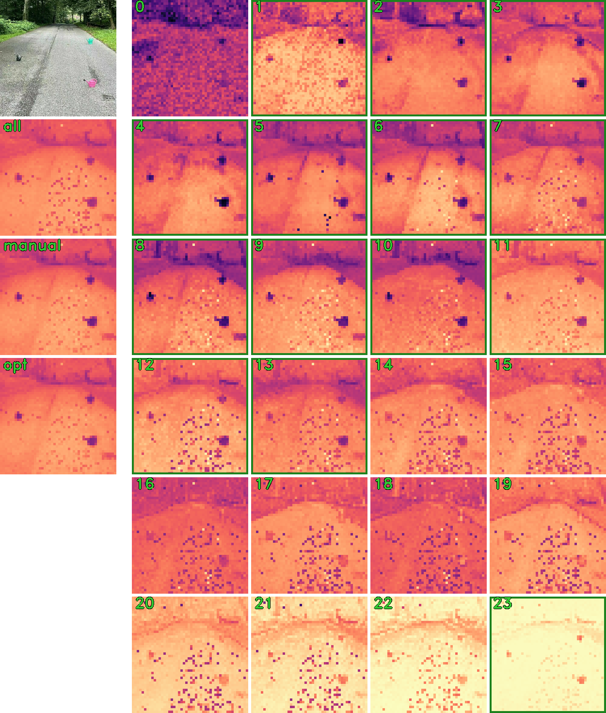
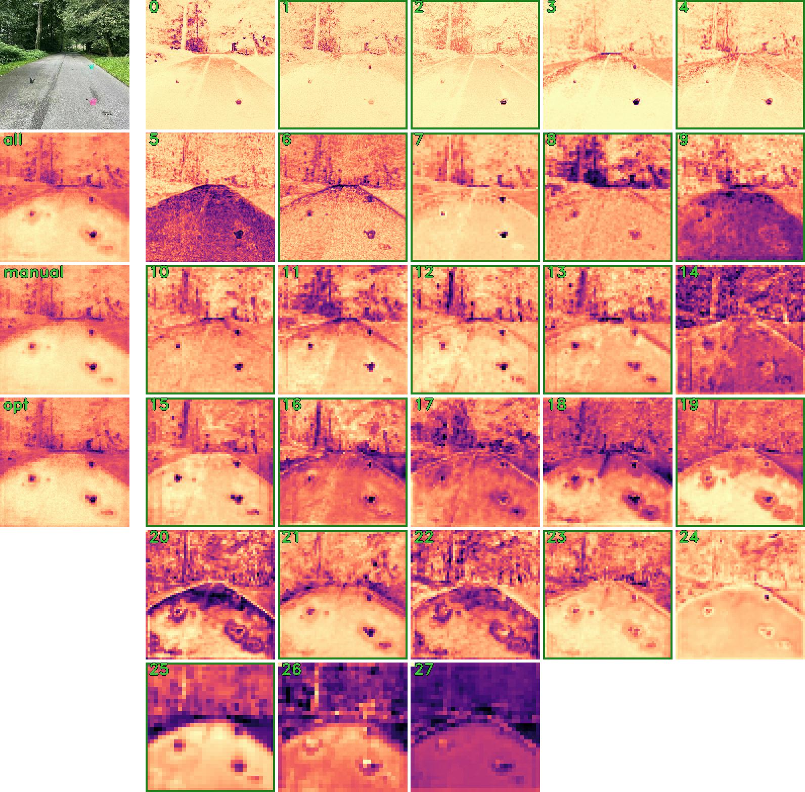
SETR (Visual Transformer) Segformer

Figure 2: Attention-entropy heatmaps for layers of SETR’s Visual Transformer and Segformer backbone. The individual layer entropies are denoted with a 0-based layer index. We observe that not all layers are equally useful for segmenting obstacles from the road. Based on visual inspection of examples, we select a subset of useful layers, marked here by a green border. In the case of SETR, roughly the earlier half of them (except the 0-th layer) exhibit distinctly low entropy in the regions of obstacles. The attention of the later layers becomes less localized and so the entropy differences across the image decrease. Segformer’s layers do not form such a clear pattern, but still its layers vary in the extent to which their entropies segment the obstacles. Many layers have artifact tokens with concentrated attention (thus low entropy) which do not correspond to any visible object. Averaging the layers tends to suppress these noisy artifacts, as visible on the averaged heatmaps; The all, manual and optimized averaging strategies are described in Sec. 4.2.

Layer Selection and Averaging. Each self-attention layer yields its own entropy heatmap $\mathbf{E}^{l}$, as shown in Fig. 2. Inspecting the entropy heatmaps reveals that obstacle regions usually have low entropy, due to their concentrated attention. There are also some isolated patches in the foreground exhibiting lower or higher entropy than their neighbourhood despite being usual parts of the road. We find that averaging entropy across layers tends to suppress these artifacts.

The entropy segments the obstacles in roughly the first half of the layers of the ViT backbone. In our experiments, we have observed that the attention maps of those layers are driven primarily by spatial closeness and visual similarity. The second half of these layers, further removed from the initial spatial embedding, appear to lose this property. Hence the obstacle segmentation capability can be further improved by selecting a subset $\mathcal{L}\subseteq\{1,\ldots,l\}$ of layer entropy heatmaps and averaging, i.e., computing

$$\frac{1}{L}\sum_{l\in\mathcal{L}}\mathbf{E}^{l}\,.$$ (9)

We study the following strategies:

• The average of all layers’ entropy heatmaps $\mathbf{E}^{l}$, i.e., $\mathcal{L}=\{1,\ldots,l\}$;

• The average of a subset of layers selected manually based on the above observation;

• A data-driven approach where we optimize linear combination weights for different layers based on training data, i.e., $\sigma(\sum_{l\in\mathcal{L}}a_{l}\mathbf{E}^{l}+b\mathbf{1})$ where $\sigma$ is the sigmoid activation, $a_{l},b\in\mathbb{R}$ and $\mathbf{1}\in\mathbb{R}^{N\times N}$ is the matrix with all elements equal to one.

Segmentation of Entropy Heatmaps. The averaged entropy is used as an obstacle detection heatmap with minimal postprocessing. Firstly, we negate the entropy since obstacles exhibit lower entropy than their surroundings. Then we linearly interpolate the entropy signal from the original resolution of $N\times N$ to a per pixel heatmap in the resolution of the input image. Choosing a threshold for the heatmap is a tradeoff between precision and recall, therefore in the evaluations we report the AuPRC over all possible thresholds.

3.3 Implementation

In practice, we use the semantic segmentation transformers SETR [43] and Segformer [41] implemented in the MMSegmentation framework [11]. Both have been trained for semantic segmentation with the Cityscapes [12] dataset. As both architectures are designed to operate on square images, sliding window inference is automatically performed on our rectangular images.

In the case of SETR [43] , we extract the attention maps from its ViT backbone. We discard the class token leaving the patch-to-patch attention and calculate Shannon entropy for each patch. Entropy from each layer has the resolution of $48\times 48$ and we perform linear interpolation to upscale it to the input image resolution. We use the PUP variant of SETR decoder head as it has the best reported segmentation performance.

The Segformer [41] uses a pyramid of self-attention operations with the base of the pyramid comprising $256^{2}$ patches. We use the MIT-B3 variant as a compromise between performance and computation cost. It would not be feasible to calculate attention between each pair of patches. Hence it performs a linear operation reducing $r$-times the number of rows of $K$ and $V$, where $r$ is a chosen reduction ratio. As a consequence, the attention matrices $A^{l}_{i}$ have only $\frac{N^{2}}{r}$ rows instead of $N^{2}$. This essentially means the attention map’s resolution is reduced. Nevertheless, we can calculate entropy over each row of $\overline{A}^{l}$, upscale the heatmaps to a common shape and average them. The number of tokens, and thus the resolution of the entropy maps, varies across layers from $256\times 256$ to $32\times 32$. We linearly interpolate all of them to $256\times 256$ before averaging, then resize the average heatmap to full image resolution.

4 Experiments

In this section we first demonstrate that the attention layers carry the required information to segment small objects for which the network has not been specifically trained. We then present results on benchmark datasets for road-obstacle detection that show that attention information is much more powerful than other widely used training-free measures such as softmax outputs and other latent features.

4.1 Datasets

This study has been motivated by need to detect road obstacles that can constitute a danger to self-driving vehicles. We therefore primarily evaluate our proposed technique for this purpose. This task is hard because there are very many different objects that might be left on the road and no training dataset set can possibly account for all of them. The commonly used benchmark datasets therefore contain obstacles which are not represented in standard training sets like Cityscapes [12].

Segment Me If You Can [7] is a benchmarking framework for the segmentation of traffic anomalies and obstacles. We test with its Road Obstacles 21 track, a dataset of diverse and small obstacles located within a variety of road scenes, including difficult weather and low light. The ground truth labels are kept private so no training can be performed on the test set. We follow the benchmark’s evaluation protocol and metrics, which measure the accuracy of classifying pixels as belonging to obstacles or the road surface, as well as object-level detection measures.

Lost and Found [34] also features obstacles on road surfaces, with a region of interest constrained to the drivable space. The background streets and parkings are relatively similar to that of Cityscapes training data. The test no known is the testing subset used in the Segment Me benchmark by excluding Cityscapes classes.

MaSTr1325 [4] contains images of maritime scenes viewed from a small unmanned surface vessel with semantic segmentation labels for water, sky and obstacles.

Airbus Aircraft Segmentation [17] features satellite images of airports. Our networks are not trained for these environment. Instead we apply SETR and Segformer with publicly available Cityscapes checkpoints.

4.2 A Layer-wise Study

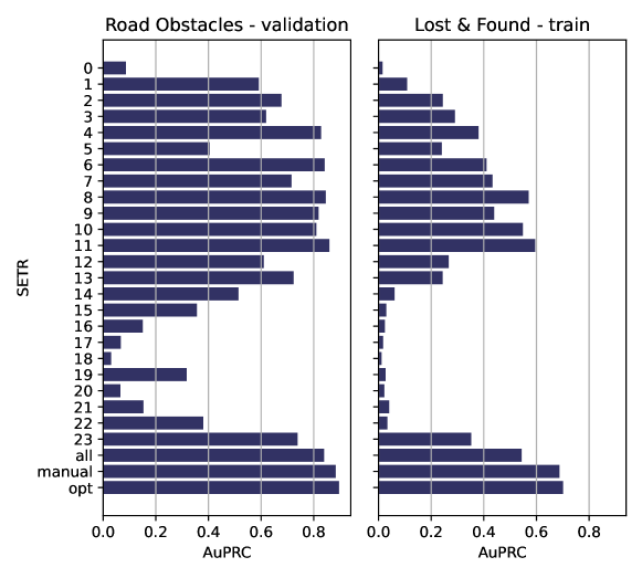
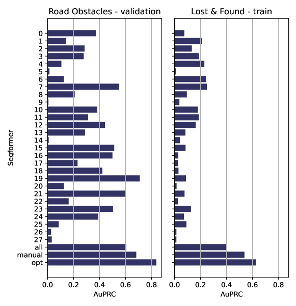
Figure 3: Usefulness of individual layers’ entropy for obstacle detection, measured by the area under the precision-recall curve of obstacle segmentation on Road Obstacles 21 - validation and Lost and Found - train datasets. In addition to layers denoted by their 0-based index, we list the scores for layer averaging strategies discussed in Sec. 4.2.

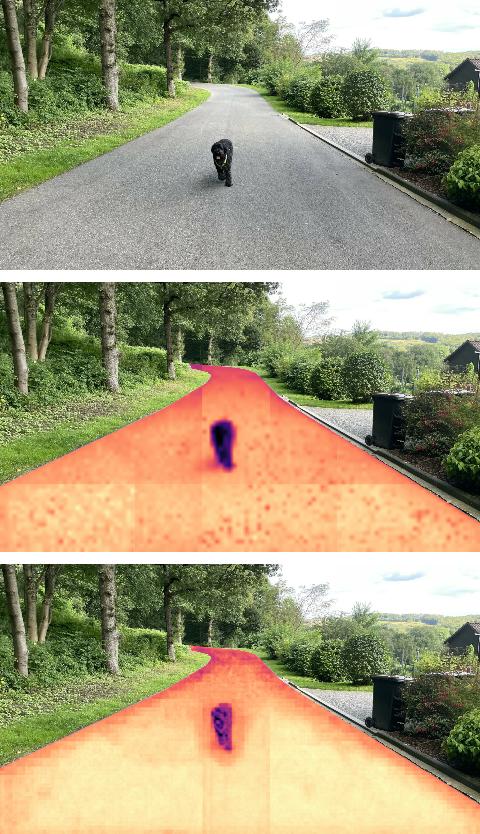
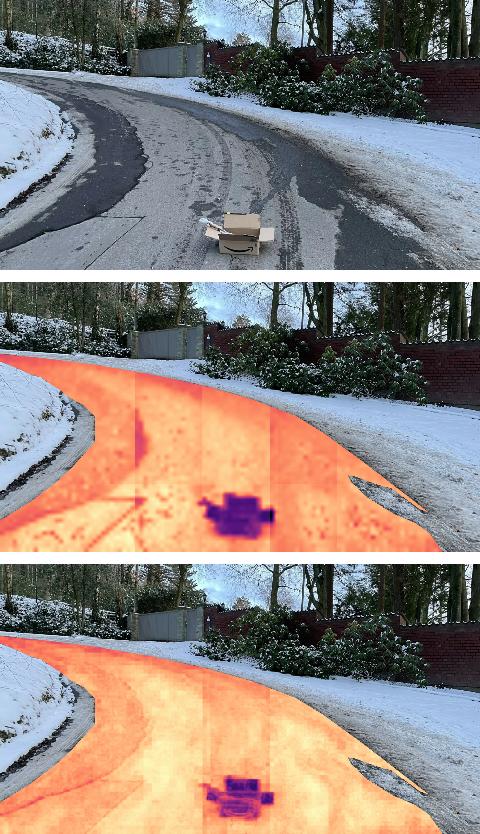
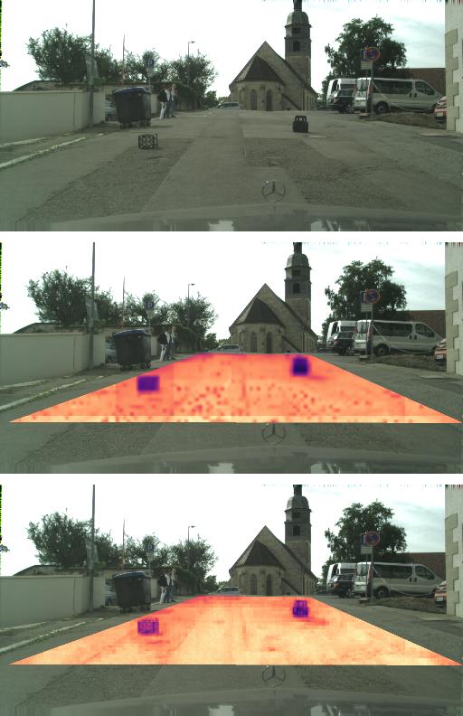
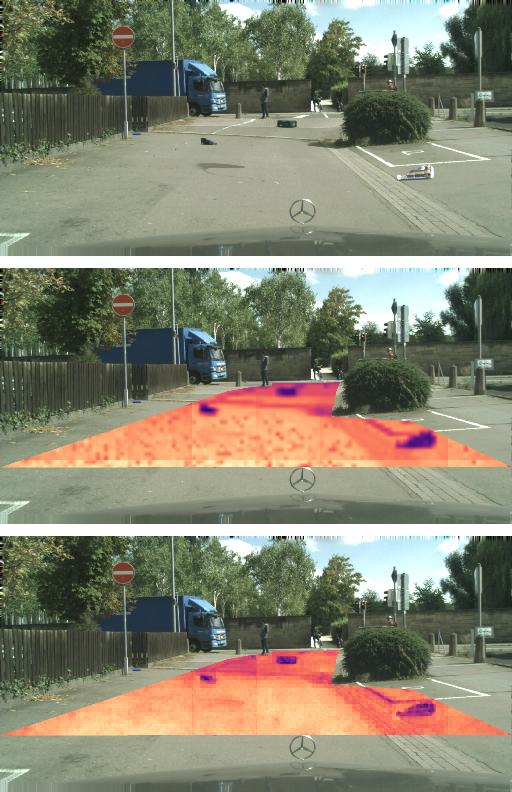
Figure 4: Qualitative results on obstacle detection in traffic scenes. The middle and bottom rows show the averaged entropy of SETR and Segformer respectively, both using manual layer averaging. The heatmap is overlaid in the evaluation ROI.

We study the usefulness of individual layers’ entropy heatmaps for obstacle detection. We measure the area under the precision-recall curve of obstacle segmentation on Road Obstacles’ validation set and Lost and Found’s training set – those datasets have publicly available obstacle labels and do not intersect with the benchmark test sets used for later comparisons. We plot the layers’ scores in Fig. 3, together with scores calculated for the following averaging strategies:

• all layers: the output heatmap is the average of all attention-entropy layers.

• manual layers: we average a subset of layers whose entropy corresponds well to obstacles, the choice is done by visual inspection of example outputs. The chosen layers are highlighted in Fig. 2.

• optimized weights: we use logistic regression to determine the optimal weights of mixing layer entropy heatmaps. We use the frames from Road Obstacles - Validation and Lost and Found - train.

The results confirm that averaging entropy across layers improves the detection quality over individual layers, and even simple visual choice of a subset of layers offers further improvement. This effect is particularly noticeable with Segformer.

In SETR, the useful layers are the concentrated roughly within the first half ($1\ldots 13$). We observe that for a given query patch, the attention in the earlier layers of SETR is focused relatively close to that query patch, and the range of attention increases with the layer. This pattern offers an explanation for the detection performance of the layers. In Segformer, the obstacle-detecting layers are not localized.

We test the layer averaging strategies in the Segment Me benchmark and present the results in Tab. 1. The results follow the findings described above except in case of SETR and Road Obstacles 21 - test where the regressed weights have slightly lower performance than the manually chosen layers. We believe this is due to the Road Obstacles 21 dataset being quite different from the data used to optimize the weights.

4.3 Benchmark Results

		Road Obstacles 21 - test					Lost and Found - test no known
		Pixel-level		Segment-level			Pixel-level		Segment-level
		AP $\uparrow$	FPR95 $\downarrow$	$\overline{\mbox{sIoU}}\uparrow$	$\overline{\mbox{PPV}}\uparrow$	$\overline{F_{1}}\uparrow$	AP $\uparrow$	FPR95 $\downarrow$	$\overline{\mbox{sIoU}}\uparrow$	$\overline{\mbox{PPV}}\uparrow$	$\overline{F_{1}}\uparrow$
SETR	all layers	67.0	5.8	30.6	22.1	22.2	62.2	11.2	27.4	28.2	24.9
	manual layers	72.9	2.5	36.4	47.8	41.6	73.0	2.9	37.1	42.8	38.0
	regression weights	71.2	2.3	36.6	40.9	36.9	73.7	4.6	35.4	46.6	38.4
Segformer	all layers	34.7	12.0	22.2	35.9	19.9	47.4	15.6	30.2	35.6	25.1
	manual layers	45.5	8.1	25.4	36.3	22.7	56.4	6.7	34.7	35.0	28.4
	regression weights	57.4	6.3	34.2	33.8	29.1	62.8	5.3	35.4	34.5	29.5

Table 1: Obstacle detection scores for layer averaging strategies. The primary metrics are Average Precision (AP$\uparrow$) for pixel classification and Average $F_{1}$ ($\overline{F_{1}}\uparrow$) for instance level detection. The evaluation protocol and metrics follow the Segment Me If You Can benchmark [7].

		Road Obstacles 21 - test					Lost and Found - test no known
		Pixel-level		Segment-level			Pixel-level		Segment-level
		AP $\uparrow$	FPR95 $\downarrow$	$\overline{\mbox{sIoU}}\uparrow$	$\overline{\mbox{PPV}}\uparrow$	$\overline{F_{1}}\uparrow$	AP $\uparrow$	FPR95 $\downarrow$	$\overline{\mbox{sIoU}}\uparrow$	$\overline{\mbox{PPV}}\uparrow$	$\overline{F_{1}}\uparrow$
No training	Ensemble [26]	1.1	77.2	8.6	4.7	1.3	2.9	82.0	6.7	7.6	2.7
	Embedding Density [3]	0.8	46.4	35.6	2.9	2.3	61.7	10.4	37.8	35.2	27.5
	MC Dropout [32]	4.9	50.3	5.5	5.8	1.0	36.8	35.5	17.4	34.7	13.0
	Maximum Softmax [25]	15.7	16.6	19.7	15.9	6.3	30.1	33.2	14.2	62.2	10.3
	Mahalanobis [27]	20.9	13.1	13.5	21.8	4.7	55.0	12.9	33.8	31.7	22.1
	ODIN [28]	22.1	15.3	21.6	18.5	9.4	52.9	30.0	39.8	49.3	34.5
	Ours Segformermanual	45.5	8.1	25.4	36.3	22.7	56.4	6.7	34.7	35.0	28.4
	Ours SETRmanual	72.9	2.5	36.4	47.8	41.6	73.0	2.9	37.1	42.8	38.0
Obstacle or anomaly training	Void Classifier [3]	10.4	41.5	6.3	20.3	5.4	4.8	47.0	1.8	35.1	1.9
	JSRNet [38]	28.1	28.9	18.6	24.5	11.0	74.2	6.6	34.3	45.9	36.0
	Image Resynthesis [31]	37.7	4.7	16.6	20.5	8.4	57.1	8.8	27.2	30.7	19.2
	Road Inpainting [29]	54.1	47.1	57.6	39.5	36.0	82.9	35.7	49.2	60.7	52.3
	SynBoost [15]	71.3	3.2	44.3	41.8	37.6	81.7	4.6	36.8	72.3	48.7
	Maximized Entropy [9]	85.1	0.8	47.9	62.6	48.5	77.9	9.7	45.9	63.1	49.9
	DenseHybrid [21]	87.1	0.2	45.7	50.1	50.7	78.7	2.1	46.9	52.1	52.3
	NFlowJS [19]	85.5	0.4	45.5	49.5	50.4	89.3	0.7	54.6	59.7	61.8

Table 2: Obstacle detection scores. The primary metrics are Average Precision (AP$\uparrow$) for pixel classification and Average $F_{1}$ ($\overline{F_{1}}\uparrow$) for instance level detection. The evaluation protocol and metrics follow the Segment Me If You Can benchmark [7].

We present benchmark results of our method for two datasets, RoadObstacle21 [7] and LostAndFound [35], in Tab. 2. We follow the evaluation protocol and metrics of the Segment Me If You Can benchmark [7]. The upper section of the table contains benchmark results of methods that do not train specifically for the detection of smaller road obstacles. Monte Carlo (MC) dropout and ensembles are approximations to Bayesian inference, relying on multiple inferences. All the other methods in that section, as well as ours, are purely based on post processing of either the network’s output or embedded features. In particular our method applied to the SETR model clearly outperforms all other baselines in the upper section w.r.t. both, pixel-level as well as segment level metrics. It can be observed, that the Segformer [41] variant performs slightly worse. Possible causes for the reduced performance are the sequence reduction applied to its attention layers resulting in coarse attention maps along with the fact that Segformer does not use the standard positional encoding found in most visual transformers. With the positional codes influencing query and key vectors, tokens can easily learn to focus their attention on neighbours. In lieu of such encoding, Segformer relies on $3\times 3$ convolutions, interspersed with the attention layers, to leak positional information from zero-padding on the image edges. Therefore, attention concentrations on small objects may be less likely to emerge.

We have also observed that small obstacles close to the horizon can pose problem to our method. Typically, the attention tends to concentrate in that regime of the image as the street narrows in. We expect that digging deeper into the attention structure as well as utilizing an auxiliary model supplied with our attention masks could yield a strongly performing overall system.

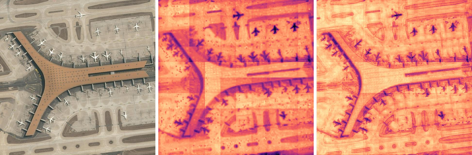
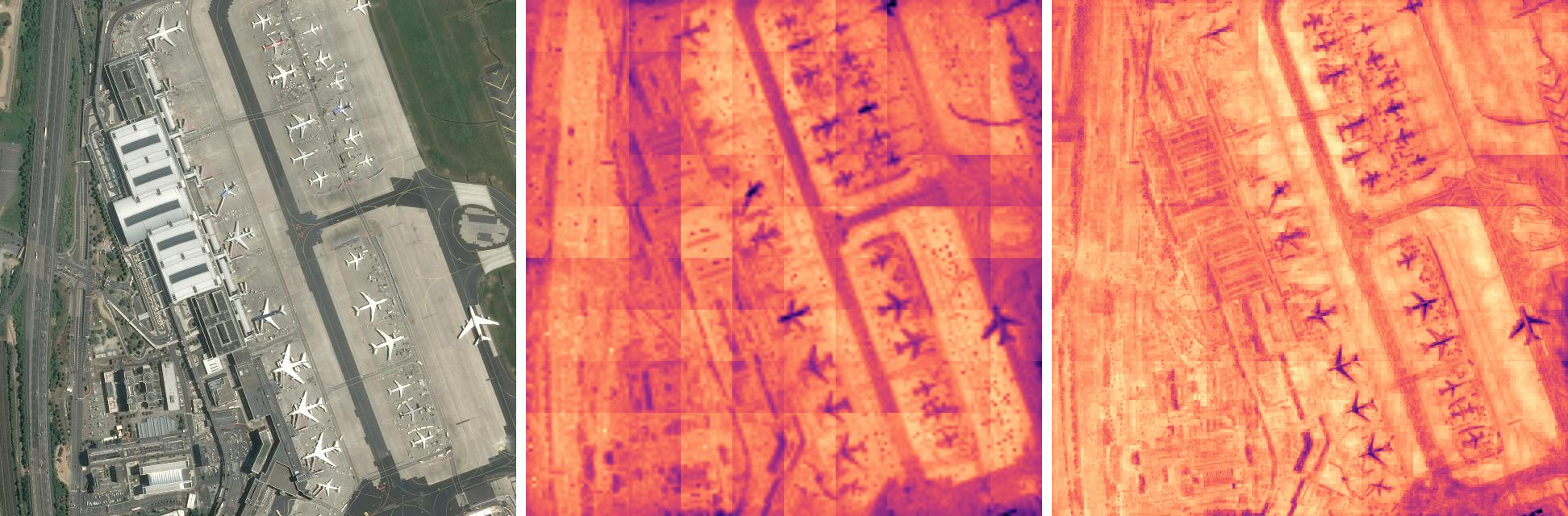
Figure 5: Qualitative results on Airbus Aircraft Detection [17] dataset. The middle and right columns show the averaged entropy of SETR and Segformer respectively.

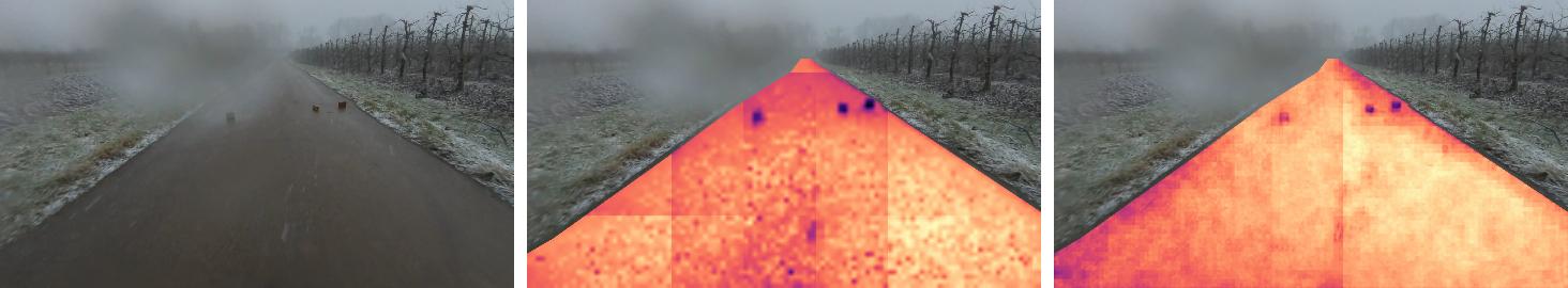
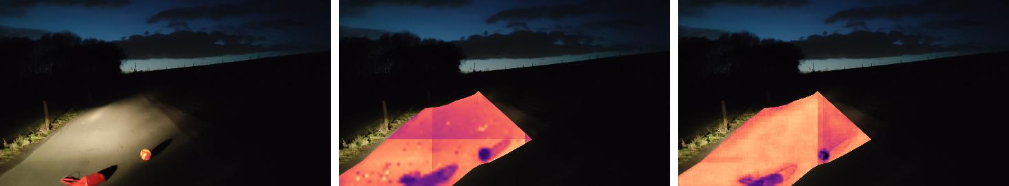
Figure 6: Qualitative results on obstacle detection in traffic scenes with difficult weather and limited light. The middle and right columns show the averaged entropy of SETR and Segformer respectively, both using manual layer averaging. Slight rectangular artifacts arise from MMSegmentation’s sliding window inference.

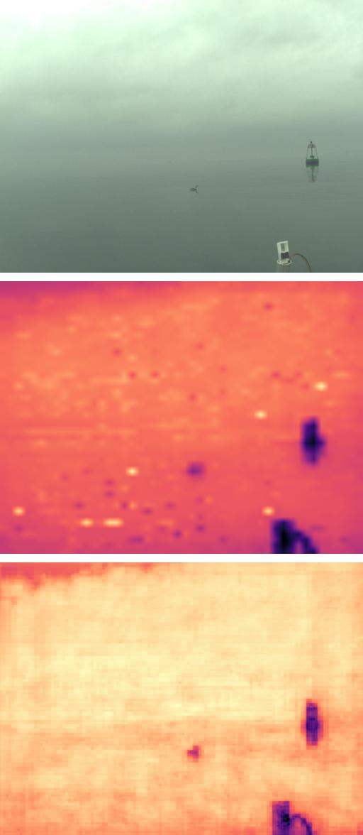
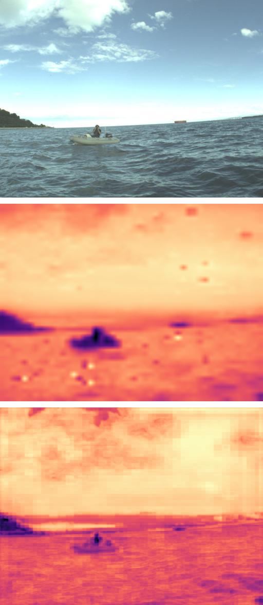
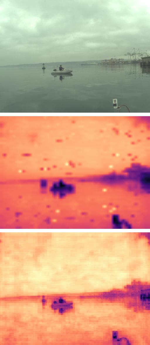
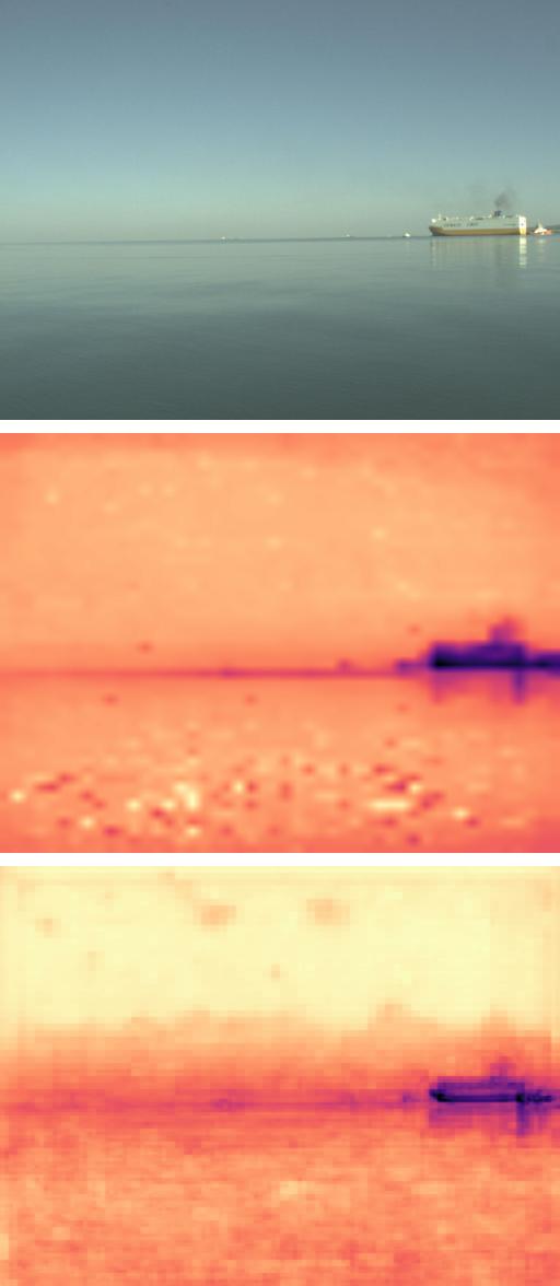
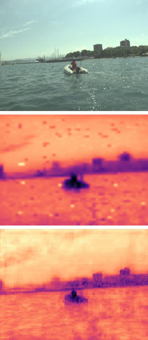
Figure 7: Qualitative results on obstacle detection in maritime scenes of the MaSTr1325 - Maritime Semantic Segmentation Training Dataset [4]. The middle and bottom rows show the averaged entropy of SETR and Segformer respectively, both using manual layer averaging. Although our networks have never been trained with maritime images, the attention entropy is still capable of detecting obstacles.

4.4 Qualitative Results and Generalization

Fig. 4 shows qualitative examples of obstacle detection in Road Obstacles and Lost and Found datasets. Objects of moderate size presented in the left-hand half of the figure can be well separated from the street. Also smaller obstacles, presented in the right-hand half of the figure are clearly visible in the heatmaps. However, it can also be noted that as the street narrows in towards the horizon, the attention concentrates more which results in a decrease of spatial entropy. These obstacles can be more difficult to detect, however, as the car approaches the obstacles, we observe that they become more clearly separable from the street. Our approach also works in difficult weather and limited light, as shown in Fig. 6. Slight rectangular artifacts arise from MMSegmentation’s sliding window inference.

Not only can the attention entropy segment previously unseen road obstacles, but its small object detection property holds in completely different domains. In the example of Fig. 7, we used the same networks trained on city scenes and ran them on maritime images from the MaSTr1325 - Maritime Semantic Segmentation Training Dataset [4]. Low attention-entropy coincides with obstacles floating on the sea, visually segmenting the obstacles very clearly. The same behavior can be observed in Fig. 5 where we performed the same experiment on images from the Airbus Aircraft Detection [17] dataset. The planes clearly stand out in the entropy maps. We expect this behavior to extends to most small salient objects visually distinct from the surrounding environment.

5 Conclusion

We performed an in-depth study of the spatial attentions of vision transformers trained for semantic segmentation [43, 41, 16]. For image patches associated to salient objects, the attention of intermediate layers tends to concentrate on that object. On the other hand, for larger areas of coherent appearance, the entropy diffuses around the given image patch under consideration. We utilized the Shannon entropy and applied it to the softmax distributions of each image patch to obtain a measure of concentration. While this measure is noisy for single layers, summing it over multiple layers helps to smooth out the noise. Applying a threshold to the heatmaps, we can accurately segment salient objects. We demonstrated this on the task of road obstacle segmentation for two different datasets [7, 34]. We outperform state-of-the-art training-free methods and get close to trained ones. Interestingly, this system can be applied out of the box on completely different tasks such as water scene segmentation, still segmenting salient objects on the water.

Appendix A Interactive attention visualization

Please view the interactive attention visualization at https://liskr.net/attentropy. Hover the cursor over the input image to choose the source patch $j$. The heatmap will display the attention values from the chosen patch $j$ to each other patch $j^{\prime}$, that is the value $\bar{A}^{l}_{j,j^{\prime}}$. The attention values are extracted from the ViT [16] backbone of the SETR [43] network, and have been truncated to the $[0,0.005]$ range for visual readability.

• By selecting a source patch within an object, we can observe how its attention is concentrated. In contrast, the road and background areas exhibit diffuse attention. This coincides with lower entropy of the attention map.

• Choose the layer shown using left and right arrow keys. We can observe how the earlier layers’ attention is spatially localized, and therefore useful for small object segmentation. The later layers show less localized attention and so we exclude them from the entropy average.

Appendix B Maritime obstacle segmentation

MaSTr1325, the Maritime Segmentation Training Dataset [4] contains images of maritime scenes viewed from a small unmanned surface vessel. The scenes contain obstacles: buoys, other boats, docks, land and so on. There are three class labels: water, sky and obstacles.

For road obstacle detectors this dataset serves as a test of generalization to very distant domain. We show qualitative segmentation performance of the training-free obstacle detection methods in Tab. 3. We do not measure object-level metrics since the maritime scenes contain non-object obstacles, such as land. Our attention entropy shows good generalization properties compared to the other methods, as shown in Fig. 8.

	AP $\uparrow$	FPR95 $\downarrow$
Ours SETRmanual	63.9	35.0
Ours Segformermanual	54.6	36.7
Maximum Softmax [25]	18.6	64.9
ODIN [28]	16.6	70.8
Mahalanobis [27]	5.9	97.3

Table 3: Obstacle pixel segmentation performance in the MaSTr1325 [4] dataset. We do not measure object-level metrics since the maritime scenes contain non-object obstacles, such as land.

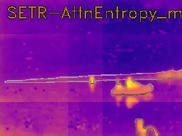
Input Ours SETR_manual

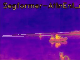
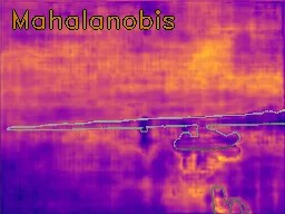
Ours Segformer_manual Mahalanobis

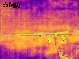
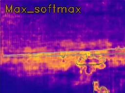
ODIN Maximum Softmax

Figure 8: Qualitative results on obstacle detection in maritime scenes of the MaSTr1325 - Maritime Semantic Segmentation Training Dataset [4]. The contour of the ground truth obstacle areas is highlighted. Compared to the other training-free obstacle detection methods, our attention entropy generalizes better to the distant domain of maritime scenes.

References

- [1] Ioannis Athanasiadis, Georgios Moschovis, and Alexander Tuoma. Weakly-supervised semantic segmentation via transformer explainability. In ML Reproducibility Challenge 2021 (Fall Edition), 2022.
- [2] Petra Bevandić, Ivan Krešo, Marin Oršić, and Siniša Šegvić. Dense open-set recognition based on training with noisy negative images. Image and Vision Computing, page 104490, 2022.
- [3] H. Blum, P.-E. Sarlin, J. Nieto, R. Siegwart, and C. Cadena. Fishyscapes: A Benchmark for Safe Semantic Segmentation in Autonomous Driving. In International Conference on Computer Vision, October 2019.
- [4] Borja Bovcon, Jon Muhovič, Janez Perš, and Matej Kristan. The MaSTr1325 dataset for training deep USV obstacle detection models. In International Conference on Intelligent Robots and Systems, 2019.
- [5] Dominik Brüggemann, Robin Chan, Matthias Rottmann, Hanno Gottschalk, and Stefan Bracke. Detecting Out of Distribution Objects in Semantic Segmentation of Street Scenes. In The 30th European Safety and Reliability Conference (ESREL), 2020.
- [6] Mathilde Caron, Hugo Touvron, Ishan Misra, Hervé Jégou, Julien Mairal, Piotr Bojanowski, and Armand Joulin. Emerging properties in self-supervised vision transformers. In Proceedings of the IEEE/CVF International Conference on Computer Vision, pages 9650–9660, 2021.
- [7] Robin Chan, Krzysztof Lis, Svenja Uhlemeyer, Hermann Blum, Sina Honari, Roland Siegwart, Pascal Fua, Mathieu Salzmann, and Matthias Rottmann. Segmentmeifyoucan: A Benchmark for Anomaly Segmentation. In Advances in Neural Information Processing Systems, 2021.
- [8] Robin Chan, Matthias Rottmann, and Hanno Gottschalk. Entropy maximization and meta classification for out-of-distribution detection in semantic segmentation. In Proceedings of the IEEE/CVF International Conference on Computer Vision (ICCV), pages 5128–5137, 10 2021.
- [9] Robin Chan, Matthias Rottmann, and Hanno Gottschalk. Entropy Maximization and Meta Classification for Out-Of-Distribution Detection in Semantic Segmentation. In International Conference on Computer Vision, 2021.
- [10] Liang-Chieh Chen, George Papandreou, Florian Schroff, and Hartwig Adam. Rethinking Atrous Convolution for Semantic Image Segmentation. In arXiv Preprint, 2017.
- [11] MMSegmentation Contributors. MMSegmentation: Openmmlab semantic segmentation toolbox and benchmark. https://github.com/open-mmlab/mmsegmentation, 2020.
- [12] Marius Cordts, Mohamed Omran, Sebastian Ramos, Timo Rehfeld, Markus Enzweiler, Rodrigo Benenson, Uwe Franke, Stefan Roth, and Bernt Schiele. The Cityscapes Dataset for Semantic Urban Scene Understanding. In Conference on Computer Vision and Pattern Recognition, 2016.
- [13] Clement Creusot and Asim Munawar. Real-Time Small Obstacle Detection on Highways Using Compressive RBM Road Reconstruction. In Intelligent Vehicles Symposium, 2015.
- [14] Jia Deng, Wei Dong, Richard Socher, Li-Jia Li, Kai Li, and Li Fei-Fei. Imagenet: A Large-Scale Hierarchical Image Database. In Conference on Computer Vision and Pattern Recognition, 2009.
- [15] Giancarlo Di Biase, Hermann Blum, Roland Siegwart, and Cesar Cadena. Pixel-Wise Anomaly Detection in Complex Driving Scenes. In Conference on Computer Vision and Pattern Recognition, June 2021.
- [16] Alexey Dosovitskiy, Lucas Beyer, Alexander Kolesnikov, Dirk Weissenborn, Xiaohua Zhai, Thomas Unterthiner, Mostafa Dehghani, Matthias Minderer, Georg Heigold, Sylvain Gelly, Jakob Uszkoreit, and Neil Houlsby. An Image is Worth 16x16 Words: Transformers for Image Recognition at Scale. In International Conference on Learning Representations, 2021.
- [17] Jeff Faudi and Airbus Defense and Space Intelligence. Airbus Aircrafts Detection Sample Dataset. https://www.kaggle.com/datasets/airbusgeo/airbus-aircrafts-sample-dataset, 2020.
- [18] Yarin Gal and Zoubin Ghahramani. Dropout as a bayesian approximation: Representing model uncertainty in deep learning. In Proceedings of The 33rd International Conference on Machine Learning, volume 48 of Proceedings of Machine Learning Research, pages 1050–1059, New York, New York, USA, 6 2016. PMLR.
- [19] Matej Grcić, Petra Bevandić, and Siniša Šegvić. Dense anomaly detection by robust learning on synthetic negative data. In arXiv Preprint, 2021.
- [20] Matej Grcic, Petra Bevandic, and Sinisa Segvic. Dense Open-set Recognition with Synthetic Outliers Generated by Real NVP. In VISIGRAPP (4: VISAPP), 2021.
- [21] Matej Grcić, Petra Bevandić, and Siniša Šegvić. DenseHybrid: Hybrid Anomaly Detection for Dense Open-Set Recognition. In ECCV, 2022.
- [22] Akshita Gupta, Sanath Narayan, KJ Joseph, Salman Khan, Fahad Shahbaz Khan, and Mubarak Shah. Ow-detr: Open-world detection transformer. In Proceedings of the IEEE/CVF Conference on Computer Vision and Pattern Recognition, pages 9235–9244, 2022.
- [23] Mark Hamilton, Zhoutong Zhang, Bharath Hariharan, Noah Snavely, and William T. Freeman. Unsupervised semantic segmentation by distilling feature correspondences. In International Conference on Learning Representations, 2022.
- [24] Dan Hendrycks, Steven Basart, Mantas Mazeika, Mohammadreza Mostajabi, Jacob Steinhardt, and Dawn Song. Scaling out-of-distribution detection for real-world settings. arXiv preprint arXiv:1911.11132, 2019.
- [25] Dan Hendrycks and Kevin Gimpel. A Baseline for Detecting Misclassified and Out-Of-Distribution Examples in Neural Networks. In International Conference on Learning Representations, 2017.
- [26] Balaji Lakshminarayanan, Alexander Pritzel, and Charles Blundell. Simple and Scalable Predictive Uncertainty Estimation Using Deep Ensembles. In Advances in Neural Information Processing Systems, 2017.
- [27] Kimin Lee, Kibok Lee, Honglak Lee, and Jinwoo Shin. A Simple Unified Framework for Detecting Out-Of-Distribution Samples and Adversarial Attacks. In Advances in Neural Information Processing Systems, pages 7167–7177, 2018.
- [28] Shiyu Liang, Yixuan Li, and R. Srikant. Enhancing the Reliability of Out-Of-Distribution Image Detection in Neural Networks. In International Conference on Learning Representations, 2018.
- [29] Krzysztof Lis, Sina Honari, Pascal Fua, and Mathieu Salzmann. Detecting Road Obstacles by Erasing Them. In arXiv Preprint, 2020.
- [30] Krzysztof Lis, Sina Honari, Pascal Fua, and Mathieu Salzmann. Perspective Aware Road Obstacle Detection. In arXiv Preprint, 2022.
- [31] Krzysztof Lis, Sina Honari, Mathieu Salzmann, and Pascal Fua. Detecting the Unexpected via Image Resynthesis. In International Conference on Computer Vision, 2019.
- [32] Jishnu Mukhoti and Yarin Gal. Evaluating Bayesian Deep Learning Methods for Semantic Segmentation. In arXiv Preprint, 2018.
- [33] Philipp Oberdiek, Matthias Rottmann, and Gernot A. Fink. Detection and retrieval of out-of-distribution objects in semantic segmentation. In Proceedings of the IEEE/CVF Conference on Computer Vision and Pattern Recognition (CVPR) Workshops, June 2020.
- [34] Peter Pinggera, Sebastian Ramos, Stefan Gehrig, Uwe Franke, Carsten Rother, and Rudolf Mester. Lost and found: detecting small road hazards for self-driving vehicles. In 2016 IEEE/RSJ International Conference on Intelligent Robots and Systems (IROS), pages 1099–1106. IEEE, 2016.
- [35] Peter Pinggera, Sebastian Ramos, Stefan Gehrig, Uwe Franke, Carsten Rother, and Rudolf Mester. Lost and Found: Detecting Small Road Hazards for Self-Driving Vehicles. In International Conference on Intelligent Robots and Systems, 2016.
- [36] Eduardo Romera, José M. Álvarez, Luis M. Bergasa, and Roberto Arroyo. ERFNet: Efficient Residual Factorized Convnet for Real-Time Semantic Segmentation. IEEE Transactions on Intelligent Transportation Systems, 2017.
- [37] Oriane Siméoni, Gilles Puy, Huy V Vo, Simon Roburin, Spyros Gidaris, Andrei Bursuc, Patrick Pérez, Renaud Marlet, and Jean Ponce. Localizing objects with self-supervised transformers and no labels. In BMVC-British Machine Vision Conference, 2021.
- [38] Tomas Vojir, Tomáš Šipka, Rahaf Aljundi, Nikolay Chumerin, Daniel Olmeda Reino, and Jiri Matas. Road Anomaly Detection by Partial Image Reconstruction with Segmentation Coupling. In International Conference on Computer Vision, October 2021.
- [39] Yangtao Wang, Xi Shen, Yuan Yuan, Yuming Du, Maomao Li, Shell Xu Hu, James L Crowley, and Dominique Vaufreydaz. Tokencut: Segmenting objects in images and videos with self-supervised transformer and normalized cut. arXiv preprint arXiv:2209.00383, 2022.
- [40] Yingda Xia, Yi Zhang, Fengze Liu, Wei Shen, and Alan Yuille. Synthesize Then Compare: Detecting Failures and Anomalies for Semantic Segmentation. In European Conference on Computer Vision, 2020.
- [41] Enze Xie, Wenhai Wang, Zhiding Yu, Anima Anandkumar, Jose M Alvarez, and Ping Luo. SegFormer: Simple and efficient design for semantic segmentation with transformers. In Advances in Neural Information Processing Systems, 2021.
- [42] Hengshuang Zhao, Jianping Shi, Xiaojuan Qi, Xiaogang Wang, and Jiaya Jia. Pyramid Scene Parsing Network. In Conference on Computer Vision and Pattern Recognition, 2017.
- [43] Sixiao Zheng, Jiachen Lu, Hengshuang Zhao, Xiatian Zhu, Zekun Luo, Yabiao Wang, Yanwei Fu, Jianfeng Feng, Tao Xiang, Philip H.S. Torr, and Li Zhang. Rethinking Semantic Segmentation from a Sequence-to-Sequence Perspective with Transformers. In CVPR, 2021.