Deep Runge-Kutta schemes for BSDEs

Abstract

We propose a new probabilistic scheme which combines deep learning techniques with high order schemes for backward stochastic differential equations belonging to the class of Runge-Kutta methods to solve high-dimensional semi-linear parabolic partial differential equations. Our approach notably extends the one introduced in [27] for the implicit Euler scheme to schemes which are more efficient in terms of discrete-time error. We establish some convergence results for our implemented schemes under classical regularity assumptions. We also illustrate the efficiency of our method for different schemes of order one, two and three. Our numerical results indicate that the Crank-Nicolson schemes is a good compromise in terms of precision, computational cost and numerical implementation.

1 Introduction

In this paper, we study the numerical approximation of Backward Stochastic Differential Equations (BSDEs for short) or equivalently semi-linear parabolic Partial Differential Equations (PDEs) by combining high order discretization schemes with deep learning techniques. We work in a Markovian setting introducing a forward diffusion process $(\mathcal{X})$ with dynamics

$$\mathcal{X}_{t}=\mathcal{X}_{0}+\int_{0}^{t}\mu(\mathcal{X}_{s})\mathrm{d}s+\int_{0}^{t}\sigma(\mathcal{X}_{s})\mathrm{d}W_{s},\,\quad 0\leq t\leq T,$$ (1.1)

and we aim to approximate the solution $(\mathcal{Y},\mathcal{Z})$ of the BSDE

$$\mathcal{Y}_{t} =g(\mathcal{X}_{T})+\int_{t}^{T}f(\mathcal{X}_{s},\mathcal{Y}_{s},\mathcal{Z}_{s})\mathrm{d}s-\int_{t}^{T}\mathcal{Z}_{s}\cdot\mathrm{d}W_{s}\,,\;0\leq t\leq T\,,$$ (1.2)

where $W$ is a $d$-dimensional Brownian motion defined on a complete probability space $(\Omega,\mathcal{A},\mathbb{P})$, $\mu:\mathbb{R}^{d}\rightarrow\mathbb{R}^{d}$ and $\sigma:\mathbb{R}^{d}\rightarrow\mathbb{M}_{d}$ (the set of $d\times d$ matrices) are measurable functions and the initial condition $\mathcal{X}_{0}$ is an $\mathbb{R}^{d}$-valued random variable independent of $W$. We denote the filtration generated by $W$ and $\mathcal{X}_{0}$ as $(\mathcal{F}_{t})_{0\leq t\leq T}$, augmented with $\mathbb{P}$ null sets.

Our approach relies on the classical connection between (BSDEs) and semi-linear parabolic PDEs as initiated in [35]. Namely, under some standard regularity assumptions on $\mu$, $\sigma$, $f$ and $g$, it holds

$$Y_{t} =u(t,\mathcal{X}_{t}),\quad Z_{t}=\sigma^{\top}(\mathcal{X}_{t})\nabla_{x}u(t,\mathcal{X}_{t}),\quad 0\leq t\leq T,$$ (1.3)

where $u:[0,T]\times\mathbb{R}^{d}\longmapsto\mathbb{R}$ is the solution to the following parabolic semi-linear PDE:

$$\left\{\begin{array}[]{ll}\partial_{t}u(t,x)+\mathcal{L}u(t,x)+f(u(t,x),\sigma^{\top}(x)\nabla_{x}u(t,x))=0,&(t,x)\in[0,T)\times\mathbb{R}^{d},\\ u(T,x)=g(x),\quad x\in\mathbb{R}^{d}&\end{array}\right.$$ (1.4)

and $\mathcal{L}$ is the infinitesimal generator defined by

$$\mathcal{L}u(t,x):=\mu(x)\cdot\nabla_{x}u(t,x)+\frac{1}{2}\mathrm{Tr}[(\sigma\sigma^{\top})(x)\nabla^{2}_{x}u(t,x)].$$ (1.5)

Since BSDEs have been introduced by Pardoux and Peng [35, 36] in 1990s, their numerical approximation has attracted considerable attention. However, solving high-dimensional BSDEs is still a challenging task. A first stream of methods relies on the backward programming algorithm (the method we study in this work belongs to this class). The main difficulty for these methods is to compute the conditional expectations. Many solutions have been proposed in the last two decades, such as the cubature methods [11, 14, 15], optimal quantization methods [2, 1, 34, 33], Malliavin calculus based methods [16, 5, 26] and some linear regression methods [20, 21, 22]. These methods are efficient in a low dimensional setting $d\sim 5$. However they all face the “curse of dimensionality”. Other type of methods have also been recently introduced, to quote a few: the branching process method (see e.g. [24]), the forward method using Wiener chaos expansion, that allows to handle possibly non Markovian setting (see e.g. [6]) and the Multi-Level Picard (MLP) method (see e.g. [28]) which does not suffer from the curse of dimensionality.

In the past five years, numerical procedures using learning methods (linear and non-linear regression) have been proposed with excellent empirical results even in high dimensional context. This includes forward schemes [17, 3, 23, 9] or backward schemes [27, 18, 37, 19], see also [7, 29, 30, 38, 12]. However, these algorithms rely on the standard Euler-Maruyama time discretization scheme whose weak convergence rate is of order 1, so that the overall computational time cost for these algorithms can still be large for high-dimensional BSDEs as many time steps might be required to achieve good accuracy.

In this paper, we combine some high-order time discretization numerical schemes for BSDEs with non-linear regression based on (deep) neural networks to solve high-dimensional semi-linear parabolic PDEs. Many high-order discrete-time approximation schemes have been introduced for BSDEs see among others [40, 41, 8, 10]. We here chose to work with the family of Runge-Kutta methods [10] which are one step schemes. It includes the implicit Euler scheme, explicit Euler scheme and the Crank-Nicolson scheme, but also schemes with more than one stage of computation per step, see Definition 2.1 below. These high-order schemes are based on a backward algorithm and, as usual, they require a good approximation procedure of conditional expectations in practice. We chose here to compute them using deep learning techniques as previous papers demonstrated their efficiency to tame the curse of dimensionality. To the best of our knowledge, high order schemes for BSDEs have not been tested with (non-linear) regression techniques. Our main contribution is thus to present an approach to implement the Runge-Kutta schemes using non-linear regression techniques in an efficient manner. Our method is inspired by the one introduced in [27] for the implicit Euler scheme. We also establish an upper-bound for the global error of our scheme which writes as the sum of the discrete time error and the approximation error induced by the use of neural networks. This is obtained by a careful analysis of the scheme, in particular its stability properties. We thus identify order one, two and three schemes whose efficiency is compared numerically. Based on our numerical experiments, we would recommend the use of the Crank-Nicolson scheme for its tractability, good precision and reasonable computational cost.

The rest of the paper is organized as follows. We first recall the definition of Runge-Kutta schemes for BSDEs in Section 2, then we study their stability in two different ways. Theorem 2.1 provides the discrete time error for the main methods that will be studied in this paper. In Section 3, we present an implementation of the Runge-Kutta schemes to solve BSDEs by neural networks, including the special case of the implicit Euler schemes [27], explicit Euler scheme, Crank-Nicolson scheme, two stage and three stage explicit Runge-Kutta scheme. We also establish the global error bound for a general learning method applied to Runge-Kutta schemes, see Theorem 3.1. In Section 4, we numerically illustrate the convergence order of the discrete time error of the methods presented in Section 3.2. We also compare the computational time cost of these methods.

We conclude this introduction by presenting some standing assumptions and notations that will be used in the sequel. From now on, we assume that the driver $f$, the terminal function $g$ and the coefficients $\mu$ and $\sigma$ of the SDE (1.1) satisfy the following regularity assumption:

Assumption 1.1.

There exists $0\leq K<\infty$ such that for all $x_{1},x_{2},z_{1},z_{2}\in\mathbb{R}^{d}$, $y_{1},y_{2}\in\mathbb{R}$

$$|f(x_{2},y_{2},z_{2})-f(x_{1},y_{1},z_{1})| \leq K\left(|x_{1}-x_{2}|+|y_{1}-y_{2}|+|z_{1}-z_{2}|\right),$$ (1.6)

$$|g(x_{2})-g(x_{1})| \leq K|x_{1}-x_{2}|,$$ (1.7)

and

$$|\mu(x_{1})-\mu(x_{2})|+|\sigma(x_{1})-\sigma(x_{2})|\leq K|x_{1}-x_{2}|.$$ (1.8)

1.1 Notations related to neural networks

We now introduce some notations and basic definitions concerning the class of neural networks that will be used in this paper:

$$\left\{\begin{array}[]{rl}\mathbb{M}_{p\times q}(\mathbb{R}):&\text{the matrix space for all }p\times q\text{ matrices with elements in }\mathbb{R},\\ d_{0}=d:&\text{input dimension,}\\ d_{1}:&\text{output dimension,}\\ L+1\in\mathbb{N}\setminus\{0,1,2\}:&\text{number of layers of the network,}\\ m_{\ell},\ell=0,1,\cdots,L:&\text{number of neurons on each layer, note }m_{0}=d_{0},m_{L}=d_{1},\\ \mathcal{H}_{n}^{\ell},\ell=1,\cdots,L-1:&\text{output of the hidden layers at time $t_{n},0\leq n\leq N-1$}.\end{array}\right.$$

For the $L-1$ hidden layers in this neural network, we choose for simplicity the same number of neurons $m_{\ell}=m,\ell=1,\cdots,L-1$.

For $\ell=1,\cdots,L$, we define the maps $\mathcal{M}_{\ell}:\mathbb{R}^{m_{\ell-1}}\longmapsto\mathbb{R}^{m_{\ell}}$ as:

$$\mathcal{M}_{\ell}(x)=\mathcal{W}_{\ell}x+\beta_{\ell},$$ (1.9)

where $\mathcal{W}_{\ell}\in\mathbb{M}_{m_{\ell}\times m_{\ell-1}}(\mathbb{R})$ is a matrix called weight, and $\beta_{\ell}\in\mathbb{R}^{m_{\ell}}$ is a vector called bias. Then $\mathcal{M}_{\ell}$ is an affine transformation that can map the features of the $(\ell-1)\verb|-|th$ layer to the $\ell\verb|-|th$ layer. A feedforward neural network is a function from $\mathbb{R}^{d_{0}}$ to $\mathbb{R}^{d_{1}}$ defined as the composition

$$\mathbb{R}^{d_{0}}\ni x\longmapsto\mathcal{N}_{m}(x;\theta)=\mathcal{M}_{L}\circ\rho_{L-1}\circ\mathcal{M}_{L-1}\circ\cdots\circ\rho_{1}\circ\mathcal{M}_{1}(x)\in\mathbb{R}^{d_{1}},$$ (1.10)

where $\rho_{\ell}(x)=(\rho(x_{1}),\cdots,\rho(x_{m_{\ell}})),x\in\mathbb{R}^{m_{\ell}},\ell=1,\cdots,L-1$, here $\rho:\mathbb{R}\longmapsto\mathbb{R}$ is an activation function which is also a nonlinear function, such as ReLu, Elu, tanh, sigmoid. Then the parameters of the neural network consist of the weight matrices $(\mathcal{W}_{\ell})_{1\leq\ell\leq L}$, the bias vector $(\beta_{\ell})_{1\leq\ell\leq L}$. For fixed $d_{0},d_{1}$ and $L$, the total number of parameters is

$$N_{m}:=\sum\limits_{\ell=1}^{L}m_{\ell}(m_{\ell-1}+1)=d_{0}(1+m)+m(m+1)(L-2)+m(1+d_{1}),$$

so that the parameters can be identified with an element $\theta\in\mathbb{R}^{N_{m}}$. We will sometimes insist on the output dimension of the neural network by using $N_{m}^{d_{1}=q}$, for a $q$ dimensional output. In particular, let us mention that for Euler schemes, the output dimension is $d_{1}:=1+d$ which includes one component for the $Y-$part and $d$ components for the $Z-$part. But for general Runge-Kutta schemes, we will set $d_{1}:=1+2d$ for the networks: The components consist $1,d,d$ dimensions for $Y,Z,A$, respectively, where $A$ is an extra $d-$dimensional variable that will be required to define the scheme, see Section 3.1.

We introduce

$$\mathcal{S}_{d_{0},d_{1},L,m}^{\rho}(\mathbb{R}^{N_{m}}):=\big{\{}\mathcal{N}_{m}(\cdot;\theta):\mathbb{R}^{d}\rightarrow\mathbb{R}^{d_{1}}\quad|\quad\theta\in\mathbb{R}^{N_{m}}\big{\}}$$ (1.11)

and

$$\mathcal{S}_{d_{0},d_{1},L}^{\rho}:=\bigcup_{m\in\mathbb{N}^{+}}\mathcal{S}_{d_{0},d_{1},L,m}^{\rho}(\mathbb{R}^{N_{m}}).$$ (1.12)

We conclude this introductory section by recalling the fundamental result of Hornik et al. [25] that states the following universal approximation theorem and justifies that the neural networks can be applied as function approximators:

Theorem 1.1 (Universal approximation theorem).

$\mathcal{S}_{d_{0},d_{1},L}^{\rho}$ is dense in $L^{2}(\upsilon)$ for any finite measure $\upsilon$ on $\mathbb{R}^{d}$, whenever $\rho$ is continuous and non-constant.

2 Runge-Kutta schemes for BSDEs

We work with the class of Runge-Kutta schemes that have been introduced in [10] in the BSDE setting. The main difference with our approach is that we also consider an approximation of the forward process. In this section, we first recall the definition of the Runge-Kutta schemes for BSDEs. We then study the stability properties of this class of scheme. We conclude the section by analyzing the discrete time error of the main schemes of interest.

2.1 Definitions

For ease of presentation, we consider an equidistant time grid

$$\pi:=\{t_{0}=0<\cdots<t_{n}<\cdots<t_{N}=T\}$$

of the interval $[0,T]$ with time step $h:=\frac{T}{N},t_{n}=nh,n=0,\cdots,N$ and let $\Delta W_{n}=W_{t_{n+1}}-W_{t_{n}},0\leq n\leq N-1$.

The Runge-Kutta schemes involve in full generality intermediate steps of computation between two dates of the main grid $\pi$. Thus, for a positive integer $Q$, let $c=(c_{1},\ldots,c_{Q+1})\in[0,1]^{Q+1}$ satisfying $0=:c_{1}<c_{2}\leq\ldots\leq c_{q}\leq\cdots\leq c_{Q}\leq c_{Q+1}:=1$. We introduce the intermediate “instances” $t_{n,q}:=t_{n+1}-c_{q}h$, for $0\leq n\leq N-1$. With these notations, we observe that $t_{n}=t_{n,Q+1}\leq\ldots\leq t_{n,q}\leq\ldots\leq t_{n,1}=t_{n+1}$. We denote the “full grid”

$$\Pi:=\{t_{n,q}\in[0,T]\,|\,0\leq n\leq N-1,1\leq q\leq Q+1\}.$$

First, we are given an approximation of the forward component (1.1) on the grid $\Pi$. Namely, for $t_{n,q}\in\Pi$, $\mathcal{X}_{t_{n,q}}$ is approximated by $X_{n,q}\in\mathcal{L}^{2}(\mathcal{F}_{t_{n,q}})$, $0\leq n\leq N-1$ and $1\leq q\leq Q+1$. For ease of notation, we will simply denote by $(X_{n})_{0\leq n\leq N}$ the approximation of $\mathcal{X}$ on the grid $\pi$. Observe that $X_{n,Q+1}=X_{n}$ and $X_{n,1}=X_{n+1}$, for $0\leq n\leq N-1$. In the following, we assume that $X$ is a Markov process on $\Pi$. We denote $\Delta W_{n,q}=W_{t_{n+1}}-{\color[rgb]{0,0,0}W_{t_{n,q}}},0\leq n\leq N-1$, $1\leq q\leq Q+1$.

We now define $(Y,Z)$ the approximation of $(\mathcal{Y},\mathcal{Z})$ given by (1.2).

Definition 2.1.

1. Assuming that $g$ is differentiable, we set the terminal condition to

   $$(Y_{N},Z_{N})=(g(X_{N}),\sigma(X_{N})^{\top}\nabla_{x}g(X_{N})).$$

2. For $0\leq n\leq N-1$ and $Q\geq 1$, the transition from $(Y_{n+1},Z_{n+1})$ to $(Y_{n},Z_{n})$ involves $Q$ stages. At the intermediate instances, for $1<q\leq Q+1$, let

   $$Y_{n,q} =\mathbb{E}_{t_{n,q}}\!\!\left[Y_{n+1}+h\sum_{k=1}^{q}a_{qk}f(X_{n,k},Y_{n,k},Z_{n,k})\right],$$ (2.1)

   $$Z_{n,q} =\mathbb{E}_{t_{n,q}}\!\!\left[H_{q}^{n}Y_{n+1}+h\sum_{k=1}^{q-1}\alpha_{qk}H_{q,k}^{n}f(X_{n,k},Y_{n,k},Z_{n,k})\right],$$ (2.2)

   where $(a_{qk})_{1\leq q,k\leq Q+1},(\alpha_{qk})_{1\leq q,k\leq Q+1}$ take their values in $\mathbb{R}$ and with $a_{1k}=\alpha_{1k}=0,1\leq k\leq Q$, $a_{qk}=\alpha_{qk}=0,1\leq q<k\leq Q+1$ and

   $$\sum_{k=1}^{q}a_{qk}=\sum_{k=1}^{q-1}\alpha_{qk}\mathbbm{1}_{\{c_{k}<c_{q}\}}=c_{q},\qquad q\leq Q+1.$$ (2.3)

   We then set $(Y_{n},Z_{n})=(Y_{n,Q+1},Y_{n,Q+1})$, for $0\leq n\leq N-1$.
   For any $1\leq k<q\leq Q+1$, $0\leq n\leq N-1$, the random variables $H_{q}^{n},H_{q,k}^{n}$ are $\mathcal{F}_{t_{n+1}}-$measurable and satisfy:

   $$\mathbb{E}_{t_{n,q}}\!\!\left[H_{q}^{n}\right]=\mathbb{E}_{t_{n,k}}\!\!\left[H_{q,k}^{n}\right]=0\text{ and }\upsilon^{n}_{q}:=\mathbb{E}_{t_{n,q}}\!\!\left[|H_{q}^{n}|^{2}\right],\upsilon^{n}_{q,k}:=\mathbb{E}_{t_{n,k}}\!\!\left[|H_{q,k}^{n}|^{2}\right],$$ (2.4)

   $$\mathbb{E}_{t_{n,q}}\!\!\left[H_{q}^{n}\Delta W_{n,q}\right]=1,$$ (2.5)

   $$\frac{\lambda}{h}\leq\min(\upsilon^{n}_{q},\upsilon^{n}_{q,k})\text{ and }\max(\upsilon^{n}_{q},\upsilon^{n}_{q,k})\leq\frac{\Lambda}{h},$$ (2.6)

   where $\lambda,\Lambda$ are positive constants which do not depend on $h$.
   

We observe that (2.5) is mainly a renormalisation property that will ease the presentation of our method. We note also that (2.1) may define $Y_{n,q}$ implicitly. For the rest of the paper, we assume

$$\max\limits_{1<q<Q+1}|a_{qq}|hK<1,$$ (2.7)

which guarantees that the scheme is well-defined, where $K$ is defined by (1.6). In particular, by a direct induction argument, it holds

$$\max_{n,q}\mathbb{E}\!\!\left[|Y_{n,q}|^{2}+|Z_{n,q}|^{2}\right]<+\infty\,.$$ (2.8)

2.2 Stability of Runge-Kutta scheme

A key property to obtain the convergence results stated in Theorem 2.1 is – classically – the $L^{2}$-stability of the schemes of Definition 2.1. This has already been observed in [10]. We shall review here this property as it will be useful in the sequel.

The first observation is the fact that the schemes given in Definition 2.1 can be written in the following implicit form, for $0\leq n\leq N-1$:

$$Y_{n} =\mathbb{E}_{t_{n}}\!\!\left[Y_{n+1}+\Phi^{Y}_{n}(Y_{n+1},Z_{n+1},h)\right],$$ (2.9)

$$Z_{n} =\mathbb{E}_{t_{n}}\!\!\left[H_{Q+1}^{n}Y_{n+1}+\Phi^{Z}_{n}(Y_{n+1},Z_{n+1},h)\right],$$ (2.10)

where $(\Phi^{Y}_{n},\Phi^{Z}_{n}):\Omega\times\mathcal{L}^{2}(\mathcal{F}_{t_{n+1}})\times\mathcal{L}^{2}(\mathcal{F}_{t_{n+1}})\times\mathbb{R}_{+}\rightarrow\mathcal{L}^{2}(\mathcal{F}_{t_{n+1}})$. This writing really stresses the fact that the schemes are one-step scheme. One introduces a perturbed version of the scheme, namely,

$$\check{Y}_{n} =\mathbb{E}_{t_{n}}\!\!\left[\check{Y}_{n+1}+\Phi^{Y}_{n}(\check{Y}_{n+1},\check{Z}_{n+1},h)\right]+\check{\zeta}^{Y}_{n}$$ (2.11)

$$\check{Z}_{n} =\mathbb{E}_{t_{n}}\!\!\left[H_{Q+1}^{n}\check{Z}_{n+1}+\Phi^{Z}_{n}(\check{Y}_{n+1},\check{Z}_{n+1},h)\right]+\check{\zeta}^{Z}_{n}$$ (2.12)

for $(\check{\zeta}^{Y}_{n},\check{\zeta}^{Z}_{n})\in\mathcal{L}^{2}(\mathcal{F}_{t_{n}})\times\mathcal{L}^{2}(\mathcal{F}_{t_{n}})$, and obtains, using Theorem 1.2(i) in [10], the following stability result, setting $\delta Y_{n}:=\check{Y}_{n}-Y_{n}$, $\delta Z_{n}:=\check{Z}_{n}-Z_{n}$,

$$\max_{n<N}{\mathbb{E}\!\!\left[|\delta Y_{n}|^{2}\right]}+\sum_{n=0}^{N-1}h\mathbb{E}\!\!\left[|\delta Z_{n}|^{2}\right]\leq C\mathbb{E}\!\!\left[|\delta Y_{N}|^{2}+h{|\delta Z_{N}|^{2}}+\sum_{n=0}^{N-1}\frac{|\check{\zeta}^{Y}_{n}|^{2}}{h}+h|\check{\zeta}^{Z}_{n}|^{2}\right]\,.$$ (2.13)

This approach is particularly well-suited for the study of the discrete time error, see the proof of Theorem 2.1 in Section 2.3 below. However, we need also a stability result to control the error linked to the estimation of the conditional expectations at each stage of the schemes. To this end, we now introduce another perturbed scheme, for $0\leq n\leq N-1$, at the intermediate instances, for $1<q\leq Q+1$, let

$$\tilde{Y}_{n,q} =\mathbb{E}_{t_{n,q}}\!\!\left[\tilde{Y}_{n+1}+h\sum_{k=1}^{q}a_{qk}f(X_{n,k},\tilde{Y}_{n,k},\tilde{Z}_{n,k})\right]+\zeta^{y}_{n,q},$$ (2.14)

$$\tilde{Z}_{n,q} =\mathbb{E}_{t_{n,q}}\!\!\left[H_{q}^{n}\tilde{Y}_{n+1}+h\sum_{k=1}^{q-1}\alpha_{qk}H_{q,k}^{n}f(X_{n,k},\tilde{Y}_{n,k},\tilde{Z}_{n,k})\right]+\zeta^{z}_{n,q},$$ (2.15)

with $(\zeta^{y}_{n,q},\zeta^{z}_{n,q})\in\mathcal{L}^{2}(\mathcal{F}_{t_{n,q}})$.

Associated to the above perturbed version, we can state the following stability result, whose proof is postponed to the Appendix, see Section 5.1.

Proposition 2.1.

Let $\delta Y_{n}:=\tilde{Y}_{n}-Y_{n}$, $\delta Z_{n}:=\tilde{Z}_{n}-Z_{n}$. There exists $0\leq C<\infty$ such that for $h$ small enough, it holds

$$\max_{0\leq n\leq N-1}{\mathbb{E}\!\!\left[|\delta Y_{n}|^{2}\right]}+\sum_{n=0}^{N-1}h\mathbb{E}\!\!\left[|\delta Z_{n}|^{2}\right]\leq C\mathbb{E}\!\!\left[|\delta Y_{N}|^{2}+h{|\delta Z_{N}|^{2}}+\sum_{n=0}^{N-1}\sum_{q=2}^{Q+1}\left(\frac{|\zeta^{y}_{n,q}|^{2}}{h}+h|\zeta^{z}_{n,q}|^{2}\right)\right]\,.$$ (2.16)

2.3 Discrete time error

In [10], the discrete-time error has been studied when $X=\mathcal{X}$, namely there is no error in the approximation of the underlying process. Building on the results in [10], we will give an upper bound of the discrete-time error when the forward process is itself approximated. We will focus here on one stage schemes both implicit and explicit and two and three stage explicit schemes. We refer to Remark 2.1 for more details on this limitation. The control of the discrete-time error is based on smoothness assumptions satisfied by the value function $u$ solution to (1.4). We now introduce the necessary notations to formalise our statement.

Let

$$\mathcal{M}:=\{\emptyset\}\cup\bigcup_{m=1}^{\infty}\{0,\dots,d\}^{m},$$

the set of multi-indices with entry $0,\dots,d$. We define the differential operators as

$$\mathcal{L}^{(0)} :=\partial_{t}+\sum_{i=1}^{d}\mu_{i}\partial_{x_{i}}+\frac{1}{2}\sum_{i=1}^{d}\sum_{j=1}^{d}(\sigma\sigma^{\top})_{ij}\partial_{x_{i},x_{j}}^{2}=\partial_{t}+\mathcal{L},$$ (2.17)

$$\mathcal{L}^{(\ell)} :=\sum_{k=1}^{d}\sigma_{k\ell}\partial_{x_{k}},\qquad\ell\in\{1,\ldots,d\},$$ (2.18)

and their iteration, namely, for $\alpha\in\mathcal{M}$,

$$\mathcal{L}^{\alpha}:=\mathcal{L}^{(\alpha_{1})}\circ\dots\circ\mathcal{L}^{(\alpha_{p})},$$

for a multi-index $\alpha$ with positive length $\mathfrak{l}(\alpha):=p$. By convention, $L^{\emptyset}$ is the identity operator ($\mathfrak{l}(\emptyset)=0$), and denote $\alpha=(0,\cdots,0)=:(0)_{p}$ with positive length $\mathfrak{l}(\alpha)=p$. By convention, we set $(0)_{0}:=\emptyset$. We denote by $*$ the concatenation of two multi-indices namely $\alpha*\beta=(\alpha_{1},\dots,\alpha_{p},\beta_{1},\dots,\beta_{q})$ with positive length $p=\mathfrak{l}(\alpha)$ and positive length $q=\mathfrak{l}(\beta)$. We set $\emptyset*\alpha=\alpha*\emptyset=\alpha$, for all $\alpha\in\mathcal{M}$. We denote by $\mathcal{G}_{b}^{l}$ the set of all functions $v:[0,T]\times\mathbb{R}^{d}\longmapsto\mathbb{R}$ for which $\mathcal{L}^{\alpha}v$ is well defined, continuous and bounded for all muti-index $\alpha\in\{(\alpha_{1},\cdots,\alpha_{p})|1\leq p\leq l\}$. We also denote classicaly $\mathcal{C}^{p}_{b}$ the set of $p$ times continuously differentiable functions with all their derivatives bounded.

In particular, we shall use the following assumption, for $p=1,2,3$:

$(\mathrm{H}r)_{p}:$ The solution $u$ to the PDE (1.4) belongs to $\mathcal{G}_{b}^{p+1}$ and $f\in\mathcal{C}^{p}_{b}$.

The key to control the discrete-time error by a judicious choice of the scheme coefficients is to be able to expand the value function $u$ along the approximation scheme $X$. To this end, we introduce the following assumption for a positive integer $M$:

$(\mathrm{H}X)_{M}:$ the process $X$ satisfies, for all $v\in\mathcal{G}^{M+1}_{b}$, $0\leq n\leq N-1$, $1<q\leq Q+1$, $k\leq q$, $1\leq\ell\leq d$, denote $v^{\alpha}=\mathcal{L}^{\alpha}v$,

$$\mathbb{E}_{t_{n,q}}\!\!\left[v(t_{n,k},X_{n,k})\right]=\sum_{m=0}^{M}v^{(0)_{m}}(t_{n,q},X_{n,q})\frac{(\{c_{q}-c_{k}\}h)^{m}}{m!}+O_{{t_{n,q}}}(h^{M+1}),$$ (2.19)

$$\mathbb{E}_{t_{n,q}}\!\!\left[(H_{q}^{n})^{\ell}v(t_{n+1},X_{n+1})\right]=\sum_{m=0}^{M-1}v^{(\ell)*(0)_{m}}(t_{n,q},X_{n,q})\frac{(c_{q}h)^{m}}{m!}+O_{{t_{n,q}}}(h^{M}),$$ (2.20)

$$\mathbb{E}_{t_{n,q}}\!\!\left[(H^{n}_{q,k})^{\ell}v(t_{n+1},X_{n+1})\right]=\sum_{m=0}^{M-1}v^{(\ell)*(0)_{m}}(t_{n,q},X_{n,q})\frac{(\{c_{q}-c_{k}\}h)^{m}}{m!}+O_{{t_{n,q}}}(h^{M}),$$ (2.21)

where the notation $R=O_{t}(r)$, $r>0$, means that the random variable $R$ is such that $|R|\leq\lambda_{t}^{r}r$ with $\lambda_{t}^{r}$ is a positive random variable satisfying for all $p,r>0$

$$\mathbb{E}\!\!\left[|\lambda_{t}^{r}|^{p}\right]\leq C_{p},$$

for some constant $C_{p}<\infty$ independent of $r$. We note that (2.19) indicates that $X$ is a weak approximation scheme of order $M$ approximation [31, 10]. Conditions (2.20)-(2.21) are required to handle the error coming from the approximation of the $Z$-component.

Regarding the discrete-time error, our main result reads as follows. Define

$$(\bar{Y}_{n},\bar{Z}_{n})=(u(t_{n},X_{n}),\sigma^{\top}\nabla_{x}u(t_{n},X_{n})),$$ (2.22)

and the global discrete time error as

$$\mathcal{T}_{N}=\max_{0\leq n\leq N-1}\mathbb{E}\!\!\left[|\bar{Y}_{n}-Y_{n}|^{2}\right]+h\sum_{n=0}^{N-1}\mathbb{E}\!\!\left[|\bar{Z}_{n}-Z_{n}|^{2}\right].$$ (2.23)

As usual, we say that the scheme is of order $\mathfrak{a}\in[0,\infty)$ if $\mathcal{T}_{N}=O(h^{2\mathfrak{a}})$.

Theorem 2.1.

1. Theta-scheme (one stage scheme): Assume $(\mathrm{H}r)_{1}$ and $(\mathrm{H}X)_{1}$, the global discrete time error of Runge-Kutta scheme is at least of order 1 if

   $$a_{21}+a_{22}=1.$$

   This condition leads to the explicit Euler scheme when $a_{21}=1$ and implicit Euler scheme when $a_{22}=1$, respectively.
   

2. Crank-Nicolson scheme (one stage scheme): Assume $(\mathrm{H}r)_{2}$ and $(\mathrm{H}X)_{2}$, the global discrete time error of Runge-Kutta scheme is at least of order 2 if

   $$a_{21}=a_{22}=\frac{1}{2}\qquad and\qquad\alpha_{21}=1.$$

3. Two stage explicit scheme: Assume $(\mathrm{H}r)_{2}$ and $(\mathrm{H}X)_{2}$, the global discrete time error of Runge-Kutta scheme is at least of order 2 if $a_{22}=a_{33}=0$ and

   $$a_{21}=c_{2},\quad a_{31}=1-\frac{1}{2c_{2}},\quad a_{32}=\frac{1}{2c_{2}},\quad and\quad\alpha_{31}+\alpha_{32}\mathbbm{1}_{\{c_{2}<1\}}=1.$$

4. Three stage explicit scheme: Assume $(\mathrm{H}r)_{3}$ and $(\mathrm{H}X)_{3}$, the global discrete time error of Runge-Kutta scheme is at least of order 3 if $0<c_{2}<c_{3}\leq 1(c_{2}\neq\frac{2}{3}\;when\;c_{3}=1),a_{22}=a_{33}=a_{44}=0$ and the following conditions holds true

   $$a_{41}+a_{42}+a_{43}=1,\quad a_{42}c_{2}+a_{43}c_{3}=\frac{1}{2},$$

   $$a_{42}c_{2}^{2}+a_{43}c_{3}^{2}=\frac{1}{3},\quad a_{43}a_{32}c_{2}=a_{43}\alpha_{32}c_{2}=\frac{1}{6},$$

   $$\alpha_{41}+\alpha_{42}+\alpha_{43}\mathbbm{1}_{\{c_{3}<1\}}=1,\quad\alpha_{42}c_{2}+\alpha_{43}c_{3}\mathbbm{1}_{\{c_{3}<1\}}=\frac{1}{2}.$$

Proof. 1. We give a short proof of the discrete time error upper bound for these most interesting schemes, as it is based on the one given in [10].
Recall the definition of $(\bar{Y}_{n},\bar{Z}_{n})_{0\leq n\leq N}$ in (2.22). We observe that it can be written also as

$$\bar{Y}_{n} =\mathbb{E}_{t_{n}}\!\!\left[\bar{Y}_{n+1}+\Phi^{Y}_{n}(\bar{Y}_{n+1},\bar{Z}_{n+1},h)\right]+\check{\zeta}^{Y}_{n},$$

$$\bar{Z}_{n} =\mathbb{E}_{t_{n}}\!\!\left[H_{Q+1}^{n}\bar{Y}_{n+1}+\Phi^{Z}_{n}(\bar{Y}_{n+1},\bar{Z}_{n+1},h)\right]+\check{\zeta}^{Z}_{n}.$$

Now, thanks to assumption $(\mathrm{H}X)_{M}$ with $M=1,2,3$, one can follow the computations made in Theorem 1.3 for statement (i)-(ii), Theorem 1.5 for statement (iii) or Theorem 1.6 for statement (iv) in [10] to obtain the corresponding upper bounds for the error linked to the perturbation, namely

$$\mathbb{E}\!\!\left[\frac{|\check{\zeta}^{Y}_{n}|^{2}}{h}+h|\check{\zeta}^{Z}_{n}|^{2}\right]=O(h^{2\mathfrak{a}+1}),$$

for $\mathfrak{a}=1,2\text{ or }3$. The proof is then concluded using (2.13). $\Box$

Remark 2.1.

(i) As mentioned in [10] and contrary to the ODE case, there exists an order barrier for implicit scheme to get an order $Q+1$ scheme with a $Q-$stage scheme when $Q>1$: This is indeed the case as soon as $\partial_{z}f\neq 0$, since the scheme given in Definition 2.1 are always explicit for the $Z$-component. Hence, we only consider the explicit scheme when $Q>1$ as the implicit scheme has no advantage compared to the explicit scheme for general drivers $f$.
(ii) For the explicit Runge-Kutta scheme, we can choose the coefficients such that $\alpha_{qk}=a_{qk}$, for all $1\leq k<q\leq Q+1$.
(iii) We do not consider the case with $Q>3$ in this paper for two main reasons. First, there is an order barrier when $Q>3$ (we need more than $Q$ stage to get an order $Q$ scheme), see [10] for a proof: This will make this scheme computationally very costly. Secondly, in our numerical experiments, when setting $Q=3$, the discrete time error is extremely small even for small number of time steps $N$ so that the global error is dominated by the variance. Hence, we cannot observe the convergence order of the scheme. We refer to Section 4 for more details on this specific point.

3 A learning method for Runge-Kutta schemes

In this section, we first give a representation of the Runge-Kutta schemes in Definition 2.1 as the solution of a sequence of optimisation problems. This new representation leads naturally to the use of non-linear regression to compute the scheme in practice. This is an extension of the method proposed in [27] for the implicit Euler scheme. We are able here to work with more efficient schemes, in terms of discrete-time error. We also study the error associated to the approximation space based on Neural Networks. In particular, we show that at each stage of computation the error can be made arbitrary small by relying on the universal approximation theorem, stated in Theorem 1.1. We then present the schemes that will be studied numerically in the next section, namely: the Euler schemes, the Crank-Nicolson scheme, two-stage and three-stage explicit Runge-Kutta schemes. We also give the convergence result for these schemes.

3.1 Implementation of Runge-Kutta schemes

Our approach to implement the Runge-Kutta schemes using non-linear regression is inspired by the approach developed in [27] for the implicit Euler scheme (named DBDP1 scheme therein). However, we need to introduce extra-terms in the computations as soon as we go away from the Euler scheme (see the $A$-terms below). Moreover, we need to compute each stage iteratively.

The whole procedure is based on the following key observation.

Lemma 3.1.

For $1<q\leq Q+1$ and $0\leq n\leq N-1$, define

$$A_{n,q} =\mathbb{E}_{t_{n,q}}\!\!\left[\sum_{k=1}^{q-1}\left(a_{qk}H_{q}^{n}-\alpha_{qk}H_{q,k}^{n}\right)hf(X_{n,k},Y_{n,k},Z_{n,k})\right],$$ (3.1)

where $(Y_{n,k},Z_{n,k})$ are defined by (2.1)-(2.2). Then, the transition from step $n$ to $n-1$ in the scheme given in Definition 2.1 is solution of the following optimisation problem

$$(Y_{n,q},Z_{n,q},A_{n,q}) =\mathrm{argmin}_{(\mathfrak{y},\mathfrak{z},\mathfrak{a})\in\mathcal{L}^{2}(\mathcal{F}_{t_{n,q}})}{L}_{n,q}(\mathfrak{y},\mathfrak{z},\mathfrak{a}),$$ (3.2)

with, for some fixed $\mathfrak{c}>0$,

$$L_{n,q}(\mathfrak{y},\mathfrak{z},\mathfrak{a}) :=\mathbb{E}\!\!\left[\Big{|}Y_{n+1}+h\sum_{k=1}^{q-1}a_{qk}f(X_{n,k},Y_{n,k},Z_{n,k})-\{\mathfrak{y}-ha_{qq}f(X_{n,q},\mathfrak{y},\mathfrak{z})+(\mathfrak{z}+\mathfrak{a})\Delta W_{n,q}\}\Big{|}^{2}\right.$$

$$\left.+h\mathfrak{c}\Big{|}\mathfrak{a}-\sum_{k=1}^{q-1}\left(a_{qk}H_{q}^{n}-\alpha_{qk}H_{q,k}^{n}\right)hf(X_{n,k},Y_{n,k},Z_{n,k})\Big{|}^{2}\right].$$

Proof. We first observe that from (2.1), (2.2) and (3.1) that

$$Y_{n+1}=Y_{n,q}-h\sum_{k=1}^{q}a_{qk}f(X_{n,k},Y_{n,k},Z_{n,k})+(Z_{n,q}+A_{n,q})\Delta W_{n,q}-\Delta M_{n,q},$$ (3.3)

where $\mathbb{E}_{t_{n}}\!\!\left[\Delta M_{n,q}\right]=\mathbb{E}_{t_{n}}\!\!\left[\Delta M_{n,q}\Delta W_{n,q}\right]=0,\mathbb{E}_{t_{n}}\!\!\left[|\Delta M_{n,q}|^{2}\right]<\infty$. We also have that

$$\quad\;\mathbb{E}\!\!\left[\left|\mathfrak{a}-\sum_{k=1}^{q-1}\left(a_{qk}H_{q}^{n}-\alpha_{qk}H_{q,k}^{n}\right)hf(X_{n,k},Y_{n,k},Z_{n,k})\right|^{2}\right]$$

$$=\mathbb{E}\!\!\left[|\mathfrak{a}-A_{n,q}|^{2}+\left|A_{n,q}-\sum_{k=1}^{q-1}\left(a_{qk}H_{q}^{n}-\alpha_{qk}H_{q,k}^{n}\right)hf(X_{n,k},Y_{n,k},Z_{n,k})\right|^{2}\right]\,.$$

Inserting (3.3) into the definition of $L_{n,q}(y,z,a)$ and using the previous equality, we compute

$$\quad L_{n,q}(\mathfrak{y},\mathfrak{z},\mathfrak{a})$$

$$=\mathbb{E}\!\!\left[\Big{|}Y_{n+1}+h\sum_{k=1}^{q-1}a_{qk}f(X_{n,k},Y_{n,k},Z_{n,k})-\{\mathfrak{y}-ha_{qq}f(X_{n,q},\mathfrak{y},\mathfrak{z})+(\mathfrak{z}+\mathfrak{a})\Delta W_{n,q}\}\Big{|}^{2}\right]$$

$$+\mathfrak{c}h\mathbb{E}\!\!\left[|\mathfrak{a}-A_{n,q}|^{2}+\left|A_{n,q}-\sum_{k=1}^{q-1}\left(a_{qk}H_{q}^{n}-\alpha_{qk}H_{q,k}^{n}\right)hf(X_{n,k},Y_{n,k},Z_{n,k})\right|^{2}\right]$$

$$=\tilde{L}^{n,q}_{1}(\mathfrak{y},\mathfrak{z})+\tilde{L}^{n,q}_{2}(\mathfrak{a},\mathfrak{z})+\tilde{L}^{n,q}_{3}(\mathfrak{a})+\ell_{n,q},$$

where

$$\tilde{L}^{n,q}_{1}(\mathfrak{y},\mathfrak{z}):=\mathbb{E}\!\!\left[|Y_{n,q}-a_{qq}hf(X_{n,q},Y_{n,q},Z_{n,q})-\{\mathfrak{y}-a_{qq}hf(X_{n,q},\mathfrak{y},\mathfrak{z})\}|^{2}\right],$$ (3.4)

$$\tilde{L}^{n,q}_{2}(\mathfrak{a},\mathfrak{z}):=c_{q}h\mathbb{E}\!\!\left[|Z_{n,q}-z+A_{n,q}-\mathfrak{a}|^{2}\right],$$ (3.5)

$$\tilde{L}^{n,q}_{3}(\mathfrak{a}):=\mathfrak{c}h\mathbb{E}\!\!\left[|A_{n,q}-\mathfrak{a}|^{2}\right],$$ (3.6)

$$\ell_{n,q}=\mathbb{E}\!\!\left[|\Delta M_{n,q}|^{2}+\mathfrak{c}h\left|A_{n,q}-\sum_{k=1}^{q-1}\left(a_{qk}H_{q}^{n}-\alpha_{qk}H_{q,k}^{n}\right)hf(X_{n,k},Y_{n,k},Z_{n,k})\right|^{2}\right].$$ (3.7)

We then observe that $\tilde{L}^{n,q}_{3}(A_{n})=0$, $\tilde{L}^{n,q}_{2}(A_{n},Z_{n})=0$ and $\tilde{L}^{n,q}_{1}(Y_{n},Z_{n})=0$, so that $(Y_{n,q},Z_{n,q},A_{n,q})$ does achieve the minimum of $L_{n,q}$.
Reciprocally, any optimal solution $(\mathfrak{y}^{\star},\mathfrak{z}^{\star},\mathfrak{a}^{\star})$ must satisfy $\tilde{L}^{n,q}_{3}(\mathfrak{a}^{\star})=0,\tilde{L}^{n,q}_{2}(\mathfrak{a}^{\star},\mathfrak{z}^{\star})=0$, which implies $\mathfrak{a}^{\star}=A_{n,q},\mathfrak{z}^{\star}=Z_{n,q}$. Moreover, necessarily one has $\tilde{L}^{n,q}_{1}(\mathfrak{y}^{\star},Z_{n,q})=0$, which leads to

$$Y_{n,q}-a_{qq}hf(X_{n,q},Y_{n,q},Z_{n,q})-\{\mathfrak{y}^{\star}-a_{qq}hf(X_{n,q},\mathfrak{y}^{\star},Z_{n,q})\}=0\;.$$

Inserting (2.1) into the previous equality, we find

$$\mathfrak{y}^{\star}=\mathbb{E}_{t_{n,q}}\!\!\left[Y_{n+1}+h\sum_{k=1}^{q-1}a_{qk}f(X_{n,k},Y_{n,k},Z_{n,k})+a_{qq}hf(X_{n,q},\mathfrak{y}^{\star},Z_{n,q})\right]\;.$$

By uniqueness of the scheme definition, recall condition (2.7), we get $\mathfrak{y}^{\star}=Y_{n,q}$, which concludes the proof. $\Box$

3.1.1 Scheme definition

We now introduce the scheme that will be implemented in the next section. Our starting point is the representation of the scheme as the solution of a sequence of optimisation problem established in the previous section. From a numerical perspective, this optimisation is solved on a parametric space of approximating functions relying on the Markov property satisfied by the Runge-Kutta schemes. We employ neural network as approximating functions, recall Section 1.1.

Let $\Phi=(\Phi_{1},\cdots,\Phi_{Q+1})\in\mathcal{C}(\mathbb{R}^{d},\mathbb{R})^{Q+1}$ and $\Psi=(\Psi_{1},\cdots,\Psi_{Q+1})\in\mathcal{C}(\mathbb{R}^{d},\mathbb{R}^{d})^{Q+1}$, we introduce a generic loss function at each stage of computation $(n,q)$, $1\leq n<N$, $1<q\leq Q+1$:

$$\mathrm{L_{n,q}^{\!RK}}[\Phi,\Psi](\theta):=\mathbb{E}\!\!\left[\Big{|}\Phi_{1}(X_{n+1})+h\sum_{k=1}^{q-1}a_{qk}f(X_{n,k},\Phi_{k}(X_{n,k}),\Psi_{k}(X_{n,k}))\right.$$ (3.8)

$$\left.\quad-\{\mathcal{U}(X_{n,q};\theta)-ha_{qq}f(X_{n,q},\mathcal{U}(X_{n,q};\theta),\mathcal{V}(X_{n,q};\theta))+(\mathcal{V}(X_{n,q};\theta)+\mathcal{A}(X_{n,q};\theta))\Delta W_{n,q}\}\Big{|}^{2}\right.$$

$$\left.\quad+\mathfrak{c}h\Big{|}\mathcal{A}(X_{n,q};\theta)-\sum_{k=1}^{q-1}\left(a_{qk}H_{q}^{n}-\alpha_{qk}H_{q,k}^{n}\right)hf(X_{n,k},\Phi_{k}(X_{n,k}),\Psi_{k}(X_{n,k}))\Big{|}^{2}\right],$$

with $(\mathcal{U},\mathcal{V},\mathcal{A}):=\mathcal{N}_{m}\in\mathcal{S}_{d_{0},d_{1},L,m}^{\rho}(\mathbb{R}^{N_{m}})$, recall (1.10)-(1.11).

In the definition of $\mathrm{L_{n,q}^{\!RK}}$ above, we do not indicate, for the reader’s convenience, the dependence upon the “balance number” $\mathfrak{c}$ (which is fixed).

Definition 3.1 (Implemented Runge-Kutta scheme).

The numerical solution is computed using the following procedure:

• For $n=N$, initialize $\hat{\mathcal{U}}_{N}=g,\hat{\mathcal{V}}_{N}=\sigma^{\top}\nabla_{x}g$,

• For $n=N-1,\cdots,0$: given $(\hat{\mathcal{U}}_{n+1},\hat{\mathcal{V}}_{n+1})=:(\hat{\mathcal{U}}_{n,1},\hat{\mathcal{V}}_{n,1})$ do

  • for $1<q\leq Q+1$ given and $(\hat{\mathcal{U}}_{n,k},\hat{\mathcal{V}}_{n,k})$, $1\leq k<q$:

    • set $(\Phi_{k},\Psi_{k}):=(\hat{\mathcal{U}}_{n,k},\hat{\mathcal{V}}_{n,k})$, $1\leq k<q$, $(\Phi_{k},\Psi_{k}):=0$, $k\geq q$

    • Compute a minimizer of the loss function:

      $$\theta_{n,q}^{\star}\in\mathrm{argmin}_{\theta}\;\mathrm{L_{n,q}^{\!RK}}[\Phi,\Psi](\theta),$$ (3.9)

      where $\mathrm{L_{n,q}^{\!RK}}$ defined by (3.8).

    • set $(\hat{\mathcal{U}}_{n,q},\hat{\mathcal{V}}_{n,q},\hat{\mathcal{A}}_{n,q}):=\mathcal{N}_{m}(\cdot;\theta_{n,q}^{\star})\in\mathcal{S}_{d_{0},d_{1},L,m}^{\rho}(\mathbb{R}^{N_{m}})$, recall (1.10)-(1.11).

  • Set $(\hat{\mathcal{U}}_{n},\hat{\mathcal{V}}_{n}):=(\hat{\mathcal{U}}_{n,Q+1},\hat{\mathcal{V}}_{n,Q+1})$.

Remark 3.1.

1. Let us note that we do not have any theoretical guarantees that the minimization problems (3.9) are well-posed on the whole space $\mathbb{R}^{N_{m}}$. A sufficient (but far from being necessary) condition is the convexity and coercivity in $\theta$ of the objective loss function (3.8). However, in practical implementation, the domain is often restricted to a compact subset of $\mathbb{R}^{N_{m}}$, so that the minimization problems are always well-posed by continuity of the loss function. In the sequel, our theoretical results are obtained by assuming the well-posedness of the scheme.

2. The value of the “balance number” $\mathfrak{c}$, recall (3.8), may impact slightly the numerical results, see Figure 2 in Section 4.

3. In practice the optimisation problems are solved classically using a Stochastic Gradient Descent (SGD) procedure which is detailed in Section 4.

3.1.2 Pseudo-consistency of the implemented scheme

We study here a kind of minimal consistency of the implemented scheme in terms of approximation error made at each step.

Our first result below clarifies the error made between one step of the genuine scheme given in (2.1)-(2.2) and one step of the approximation scheme given above. As expected, this error is controlled by the approximation power of the class of DNN considered.

Lemma 3.2.

Let $0\leq n\leq N-1$ and $1<q\leq Q+1$. Let $\Phi=(\Phi_{1},\cdots,\Phi_{Q+1})\in\mathcal{C}(\mathbb{R}^{d},\mathbb{R})^{Q+1}$ and $\Psi=(\Psi_{1},\cdots,\Psi_{Q+1})\in\mathcal{C}(\mathbb{R}^{d},\mathbb{R}^{d})^{Q+1}$ and define

$${Y}^{(\Phi,\Psi)}_{n,q} :=\mathbb{E}_{t_{n,q}}\!\!\left[{Y}^{(\Phi,\Psi)}_{n,1}+h\sum_{k=1}^{q}a_{qk}f(X_{n,k},{Y}^{(\Phi,\Psi)}_{n,k},{Z}^{(\Phi,\Psi)}_{n,k})\right],$$ (3.10)

$${Z}^{(\Phi,\Psi)}_{n,q} :=\mathbb{E}_{t_{n}}\!\!\left[H^{n}_{q}{Y}^{(\Phi,\Psi)}_{n,1}+h\sum_{k=1}^{q-1}\alpha_{qk}H^{n}_{q,k}f(X_{n,k},{Y}^{(\Phi,\Psi)}_{n,k},{Z}^{(\Phi,\Psi)}_{n,k})\right],$$ (3.11)

$$A^{(\Phi,\Psi)}_{n,q} =\mathbb{E}_{t_{n,q}}\!\!\left[\sum_{k=1}^{q-1}\left(a_{qk}H_{q}^{n}-\alpha_{qk}H_{q,k}^{n}\right)hf(X_{n,k},{Y}^{(\Phi,\Psi)}_{n,k},{Z}^{(\Phi,\Psi)}_{n,k})\right],$$ (3.12)

with $({Y}^{(\Phi,\Psi)}_{n,k},{Z}^{(\Phi,\Psi)}_{n,k}):=(\Phi_{k}(X_{n,k}),\Psi_{k}(X_{n,k}))$, for $1\leq k<q$. Assume that there exists $\theta^{\star}\in\mathbb{R}^{N_{m}}$ such that

$$\theta^{\star}\in\mathrm{argmin}_{\theta}\;\mathrm{L_{n,q}^{\!RK}}[\Phi,\Psi](\theta),$$

then, there exists $C<\infty$ independent of $n$ and $q$ such that, for $h$ small enough,

$$\quad\mathbb{E}\!\!\left[|{Y}^{(\Phi,\Psi)}_{n,q}-\mathcal{U}_{n,q}(X_{n,q};\theta^{\star})|^{2}+h|{Z}^{(\Phi,\Psi)}_{n,q}-\mathcal{V}_{n,q}(X_{n,q};\theta^{\star})|^{2}+h|{A}^{(\Phi,\Psi)}_{n,q}-\mathcal{A}_{n,q}(X_{n,q};\theta^{\star})|^{2}\right]$$

$$\leq C\mathcal{E}_{n,q}(\Phi,\Psi),$$ (3.13)

where

$$\mathcal{E}_{n,q}(\Phi,\Psi)=\epsilon_{n,q}^{\mathcal{N},y}(\Phi,\Psi)+h\epsilon_{n,q}^{\mathcal{N},z}(\Phi,\Psi)+h\epsilon_{n,q}^{\mathcal{N},a}(\Phi,\Psi),$$ (3.14)

and

$$\epsilon_{n,q}^{\mathcal{N},y}(\Phi,\Psi) :=\inf_{\theta^{y}\in N_{m}^{d_{1}=1}}\mathbb{E}\!\!\left[|{Y}^{(\Phi,\Psi)}_{n,q}-\mathcal{U}_{n,q}(X_{n,q};\theta^{y})|^{2}\right],$$ (3.15)

$$\epsilon_{n,q}^{\mathcal{N},a}(\Phi,\Psi) :=\inf_{\theta^{a}\in N_{m}^{d_{1}=d}}\mathbb{E}\!\!\left[|{A}^{(\Phi,\Psi)}_{n,q}-\mathcal{A}_{n,q}(X_{n,q};\theta^{a})|^{2}\right],$$ (3.16)

$$\epsilon_{n,q}^{\mathcal{N},z}(\Phi,\Psi) :=\inf_{\theta^{z}\in N_{m}^{d_{1}=d}}\mathbb{E}\!\!\left[|{Z}^{(\Phi,\Psi)}_{n,q}-\mathcal{V}_{n,q}(X_{n,q};\theta^{z})|^{2}\right].$$ (3.17)

Proof. 1. We first observe that (3.10) rewrites

$${Y}^{(\Phi,\Psi)}_{n+1}={Y}^{(\Phi,\Psi)}_{n,q} -h\sum_{k=1}^{q}a_{qk}f(X_{n,k},{Y}^{(\Phi,\Psi)}_{n,k},{Z}^{(\Phi,\Psi)}_{n,k})+\left({Z}^{(\Phi,\Psi)}_{n}+{A}^{(\Phi,\Psi)}_{n}\right)\Delta W_{n,q}+\Delta{M}^{(\Phi,\Psi)}_{n,q}\;,$$ (3.18)

where $\mathbb{E}_{t_{n,q}}\!\!\left[\Delta M^{(\Phi,\Psi)}_{n,q}\right]=\mathbb{E}_{t_{n,q}}\!\!\left[\Delta M^{(\Phi,\Psi)}_{n,q}\Delta W_{n,q}\right]=0,\mathbb{E}_{t_{n,q}}\!\!\left[|\Delta M^{(\Phi,\Psi)}_{n,q}|^{2}\right]<\infty$. Following the same computations as in the proof of Lemma 3.1, we obtain that

$$\mathrm{L_{n,q}^{\!RK}}[\Phi,\Psi](\theta)=\tilde{L}^{n,q}_{1}[\Phi,\Psi](\theta)+\tilde{L}^{n,q}_{2}[\Phi,\Psi](\theta)+\tilde{L}^{n,q}_{3}[\Phi,\Psi](\theta)+\ell_{n,q}[\Phi,\Psi],$$ (3.19)

with

$$\tilde{L}^{n,q}_{1}[\Phi,\Psi](\theta) =\mathbb{E}\Big{[}|{Y}^{(\Phi,\Psi)}_{n,q}-a_{qq}hf(X_{n,q},{Y}^{(\Phi,\Psi)}_{n,q},{Z}^{(\Phi,\Psi)}_{n,q})$$ (3.20)

$$\qquad-\{\mathcal{U}_{n,q}(X_{n,q};\theta)-a_{qq}hf(X_{n,q},\mathcal{U}_{n,q}(X_{n,q};\theta),\mathcal{V}_{n,q}(X_{n,q};\theta))\}|^{2}\Big{]},$$

$$\tilde{L}^{n,q}_{2}[\Phi,\Psi](\theta) =c_{q}h\mathbb{E}\!\!\left[|{Z}^{(\Phi,\Psi)}_{n,q}-\mathcal{V}_{n,q}(X_{n,q};\theta)+{A}^{(\Phi,\Psi)}_{n,q}-\mathcal{A}_{n,q}(X_{n,q};\theta)|^{2}\right],$$ (3.21)

$$\tilde{L}^{n,q}_{3}[\Phi,\Psi](\theta) =\mathfrak{c}h\mathbb{E}\!\!\left[|{A}^{(\Phi,\Psi)}_{n,q}-\mathcal{A}_{n,q}(X_{n,q};\theta)|^{2}\right],$$ (3.22)

$$\ell_{n,q}[\Phi,\Psi]= \mathbb{E}\!\!\left[\mathfrak{c}h\left|{A}^{(\Phi,\Psi)}_{n,q}-\sum_{k=1}^{q-1}\left(a_{qk}H_{q}^{n}-\alpha_{qk}H_{q,k}^{n}\right)hf(X_{n,k},{Y}^{(\Phi,\Psi)}_{n,k},{Z}^{(\Phi,\Psi)}_{n,k})\right|^{2}+|\Delta M^{(\Phi,\Psi)}_{n,q}|^{2}\right].$$ (3.23)

Setting $\tilde{L}_{n,q}[\Phi,\Psi](\theta):=\tilde{L}^{n,q}_{1}[\Phi,\Psi](\theta)+\tilde{L}^{n,q}_{2}[\Phi,\Psi](\theta)+\tilde{L}^{n,q}_{3}[\Phi,\Psi](\theta)$, we then deduce that

$$\mathrm{argmin}_{\theta}\,\tilde{L}_{n,q}[\Phi,\Psi](\theta)=\mathrm{argmin}_{\theta}\,\mathrm{L_{n,q}^{\!RK}}[\Phi,\Psi](\theta).$$ (3.24)

2. From the Lipschitz continuity of $f$ and recalling (2.4)-(2.6), we directly obtain the following upper bound:

$$\tilde{L}_{n,q}[\Phi,\Psi](\theta)\leq C\mathbb{E}\!\!\left[|{Y}^{(\Phi,\Psi)}_{n,q}-\mathcal{U}_{n,q}(X_{n,q};\theta)|^{2}+h|{Z}^{(\Phi,\Psi)}_{n,q}-\mathcal{V}_{n,q}(X_{n,q};\theta)|^{2}\right.$$

$$\qquad\left.+h|{A}^{(\Phi,\Psi)}_{n,q}-\mathcal{A}_{n,q}(X_{n,q};\theta)|^{2}\right]\,.$$ (3.25)

We now prove a similar lower bound for $\tilde{L}_{n,q}[\Phi,\Psi](\theta)$. We will use the following inequality

$$(x+y)^{2}\geq x^{2}(1-\alpha)+y^{2}(1-\frac{1}{\alpha}),\quad 0<\alpha<1.$$ (3.26)

Thus, for any $\alpha$ such that $1>\alpha{\color[rgb]{0,0,0}>\frac{2c_{q}}{2c_{q}+\mathfrak{c}}}$, we obtain

$$\tilde{L}_{2}^{n,q}[\Phi,\Psi](\theta)+\tilde{L}_{3}^{n,q}[\Phi,\Psi](\theta)\geq h{\color[rgb]{0,0,0}(1-\alpha)c_{q}}\mathbb{E}\!\!\left[|{Z}^{(\Phi,\Psi)}_{n,q}-\mathcal{V}_{n,q}(X_{n,q};\theta)|^{2}\right]$$ (3.27)

$$+h\frac{{\color[rgb]{0,0,0}\mathfrak{c}}}{2}\mathbb{E}\!\!\left[|{A}^{(\Phi,\Psi)}_{n,q}-\mathcal{A}_{n,q}(X_{n,q};\theta)|^{2}\right]\,.$$

Using again (3.26) with $\alpha=1/2$ and then the fact that $f$ is Lipschitz continuous, we get

$$\tilde{L}_{1}^{n,q}[\Phi,\Psi](\theta) \geq\frac{1}{2}\mathbb{E}\!\!\left[|{Y}^{(\Phi,\Psi)}_{n,q}-\mathcal{U}_{n,q}(X_{n,q},\theta)|^{2}\right]$$

$$-a_{qq}^{2}h^{2}\mathbb{E}\!\!\left[|f(X_{n,q},{Y}^{(\Phi,\Psi)}_{n,q},{Z}^{(\Phi,\Psi)}_{n,q})-f(X_{n,q},\mathcal{U}_{n,q}(X_{n,q};\theta),\mathcal{V}_{n,q}(X_{n,q};\theta))|^{2}\right]$$

$$\geq(\frac{1}{2}-2a_{qq}^{2}L^{2}h^{2})\mathbb{E}\!\!\left[|{Y}^{(\Phi,\Psi)}_{n,q}-\mathcal{U}_{n,q}(X_{n,q},\theta)|^{2}\right]-2a_{qq}^{2}L^{2}h^{2}\mathbb{E}\!\!\left[|{Z}^{(\Phi,\Psi)}_{n,q}-\mathcal{V}_{n,q}(X_{n,q},\theta)|^{2}\right].$$

Combining the previous inequality with (3.27), we deduce that for $h$ small enough,

$$\quad\mathbb{E}\!\!\left[|{Y}^{(\Phi,\Psi)}_{n,q}-\mathcal{U}_{n,q}(X_{n,q};\theta)|^{2}+h|{Z}^{(\Phi,\Psi)}_{n,q}-\mathcal{V}_{n,q}(X_{n,q};\theta)|^{2}+h|{A}^{(\Phi,\Psi)}_{n,q}-\mathcal{A}_{n,q}(X_{n,q};\theta)|^{2}\right]$$

$$\leq C\tilde{L}_{n,q}[\Phi,\Psi](\theta)$$ (3.28)

3. The above inequality is a fortiori true at the optimum $\theta^{\star}$. Moreover, optimizing on separated networks is always more costly than optimizing on a fully connected network thus leading to (3.2). $\Box$

We conclude this section with a result expressing the global error between the scheme given in Definition 2.1 and the one given in Definition 3.1.

Proposition 3.1.

Assume that the scheme given in Definition 3.1 is well-posed then

$$\max_{0\leq n\leq N}\mathbb{E}\!\!\left[|Y_{n}-\hat{\mathcal{U}}_{n}(X_{n})|^{2}\right]+h\sum_{n=0}^{N}\mathbb{E}\!\!\left[|Z_{n}-\hat{\mathcal{V}}_{n}(X_{n})|^{2}\right]\leq CN\sum_{n=0}^{N-1}\bar{\mathcal{E}}_{n}\,,$$ (3.29)

where $\bar{\mathcal{E}}_{n}:=\sum\limits_{k=1}^{Q}\mathcal{E}_{n,k}(\hat{\Phi}_{n},\hat{\Psi}_{n})$ recalling (3.14) and with $\hat{\Phi}=(\hat{\mathcal{U}}_{n,k})_{1\leq k\leq Q}$ and $\hat{\Psi}=(\hat{\mathcal{V}}_{n,k})_{1\leq k\leq Q}$.

Proof. Let us define, for $0\leq n\leq N-1,1<q\leq Q+1$, recalling (3.10)-(3.11)-(3.12),

$$\bar{Y}_{n,q}=Y^{(\hat{\Phi},\hat{\Psi})}_{n,q}\,,\;\bar{Z}_{n,q}=Z^{(\hat{\Phi},\hat{\Psi})}_{n,q}\,,\;\bar{A}_{n,q}=A^{(\hat{\Phi},\hat{\Psi})}_{n,q}\,.$$ (3.30)

We first observe that $(\hat{U}_{n,q},\hat{V}_{n,q}):=({\color[rgb]{0,0,0}\hat{\mathcal{U}}_{n,q}(X_{n,q}),\hat{\mathcal{V}}_{n,q}(X_{n,q})})$ can be rewritten as a perturbed scheme, namely

$$\hat{U}_{n,q} =\mathbb{E}_{t_{n,q}}\!\!\left[\hat{U}_{n+1}+h\sum_{k=1}^{q}a_{qk}f(X_{n,k},\hat{U}_{n,k},\hat{V}_{n,k})\right]+\zeta^{y}_{n,q},$$ (3.31)

$$\hat{V}_{n,q} =\mathbb{E}_{t_{n,q}}\!\!\left[H_{q}^{n}\hat{U}_{n+1}+h\sum_{k=1}^{q-1}\alpha_{qk}H_{q,k}^{n}f(X_{n,k},\hat{U}_{n,k},\hat{V}_{n,k})\right]+\zeta^{z}_{n,q},$$ (3.32)

with

$$\zeta^{y}_{n,q} :=\hat{U}_{n,q}-\bar{Y}_{n,q}+a_{qq}h\left(f(X_{n,q},\bar{Y}_{n,q},\bar{Z}_{n,q})-f(X_{n,q},\hat{U}_{n,q},\hat{V}_{n,q})\right),$$ (3.33)

$$\zeta^{z}_{n,q} :=\hat{V}_{n,q}-\bar{Z}_{n,q}\,.$$ (3.34)

Indeed, with our notations, we have $(\hat{U}_{n,k},\hat{V}_{n,k})=(Y_{n,k}^{(\hat{\Phi},\hat{\Psi})},Z_{n,k}^{(\hat{\Phi},\hat{\Psi})}),1\leq k<q$. Moreover, since $\hat{U}_{n,q}=\hat{\mathcal{U}}_{n,q}(X_{n,q})={\mathcal{U}_{n,q}}(X_{n,q},\theta^{\star}_{n,q})$, recall Definition 3.1, it holds

$$\mathbb{E}\!\!\left[\frac{1}{h}|\zeta^{y}_{n,q}|^{2}+h|\zeta^{z}_{n,q}|^{2}\right] \leq C\mathbb{E}\!\!\left[\frac{1}{h}|{\mathcal{U}_{n,q}}(X_{n,q},\theta^{\star}_{n,q})-\bar{Y}_{n,q}|^{2}+h|{\mathcal{V}_{n,q}}(X_{n,q},\theta^{\star}_{n,q})-\bar{Z}_{n,q}|^{2}\right]$$

$$\leq CN\mathcal{E}_{n,q}(\hat{\mathcal{U}}_{n+1},\hat{\mathcal{V}}_{n+1}),$$

where for the last inequality we applied Lemma 3.2. Now the proof is concluded using the stability result given in Proposition 2.1. $\Box$

We conclude this section with the following result.

Theorem 3.1.

Recall the definition of $(\bar{Y}_{n},\bar{Z}_{n})_{0\leq n\leq N}$ in (2.22) and of the discrete-time error $\mathcal{T}_{N}$ in (2.23). Then, the following holds

$$\max_{n\leq N}\mathbb{E}\!\!\left[|\bar{Y}_{n}-\hat{\mathcal{U}}_{n}(X_{n})|^{2}\right]+h\sum_{n=0}^{N}\mathbb{E}\!\!\left[|\bar{Z}_{n}-\hat{\mathcal{V}}_{n}(X_{n})|^{2}\right]\leq C(\mathcal{T}_{N}+N\sum_{n=0}^{N-1}\bar{\mathcal{E}}_{n})\,,$$ (3.35)

where $\bar{\mathcal{E}}_{n}:=\sum\limits_{k=1}^{Q}\mathcal{E}_{n,k}(\hat{\Phi}_{n},\hat{\Psi}_{n})$ and with $\hat{\Phi}=(\hat{\mathcal{U}}_{n,k})_{1\leq k\leq Q}$ and $\hat{\Psi}=(\hat{\mathcal{V}}_{n,k})_{1\leq k\leq Q}$, recall (3.14).

Proof. We simply observe that

$$\quad\max_{n}\mathbb{E}\!\!\left[|\bar{Y}_{n}-\hat{\mathcal{U}}_{n}(X_{n})|^{2}\right]+\sum_{n=0}^{N-1}h\mathbb{E}\!\!\left[|\bar{Z}_{n}-\hat{\mathcal{V}}_{n}(X_{n})|^{2}\right]$$

$$\leq 2\left(\max_{n}\mathbb{E}\!\!\left[|\bar{Y}_{n}-Y_{n}|^{2}\right]+\sum_{n=0}^{N-1}h\mathbb{E}\!\!\left[|\bar{Z}_{n}-Z_{n}|^{2}\right]\right)$$

$$+2\left(\max_{n}\mathbb{E}\!\!\left[|{Y}_{n}-\hat{\mathcal{U}}_{n}(X_{n})|^{2}\right]+\sum_{n=0}^{N-1}h\mathbb{E}\!\!\left[|{Z}_{n}-\hat{\mathcal{V}}_{n}(X_{n})|^{2}\right]\right).$$

The first term in the right hand side of the previous inequality is the discrete-time error and the second term is upper bounded using Proposition 3.1. $\Box$

Remark 3.2.

1. Observe that (3.35) provides an upper-bound for the error $|\mathcal{Y}_{0}-\hat{\mathcal{U}}_{n}(X_{0})|$ at the initial time.

2. The above result is a first step only toward the proof of convergence of the implemented RK scheme. Indeed, one observes that the local error $\bar{\mathcal{E}}_{n}$ is defined using the solution computed at the previous time step. For fixed number of time steps $N$, Theorem 1.1 combined with Lemma 3.2 shows that this error can be made as small as desired. This confirms that the implemented scheme is a reasonable scheme to consider. The theoretical difficulty to obtain a full convergence result comes from the highly non linear optimisation problem that have to be solved when using deep neural networks as approximation space. From a practical point of view, next section shows that the numerical procedure associated to Definition 3.1 is efficient.

3.2 Review of classical Runge-Kutta schemes

We now present the schemes that are used to perform the numerical simulations. We will consider only the Euler schemes, the Crank-Nicholson scheme and some two-stage and three-stage explicit Runge-Kutta schemes, recall Remark 2.1.

3.2.1 Euler schemes

We first specialize the results of the previous section to the case of the Euler schemes. As already mentioned, for the implicit Euler scheme, we obtain exactly the procedure introduced in [27].

For this section, we assume that $(X_{n})_{n\leq N}$ is given by the classical Euler scheme on $\pi$:

$$X_{n+1}=X_{n}+\mu(X_{n})h+\sigma(X_{n})\Delta W_{n}\;,n\leq N-1\;,$$ (3.36)

with $\Delta W_{n}:=W_{t_{n+1}}-W_{t_{n}}$ and $X_{0}=\mathcal{X}_{0}$.

The implicit Euler scheme for BSDEs [39, 4], which is a one stage scheme, reads classically as follows, for $0\leq n<N$,

$$Y_{n}=\mathbb{E}_{t_{n}}\!\!\left[Y_{n+1}+hf(X_{n},Y_{n},Z_{n}))\right]\text{ and }Z_{n}=\mathbb{E}_{t_{n}}\!\!\left[\frac{\Delta W_{n}}{h}Y_{n+1}\right],$$ (3.37)

where we set $H_{n}=\frac{W_{t_{n+1}}-W_{t_{n}}}{h}$. We observe that (2.4)-(2.6) and (2.5) are satisfied and that $({HX})_{1}$ holds true here.

The loss function given in (3.8) simplifies here as follows: for $\varphi\in\mathcal{C}(\mathbb{R}^{d},\mathbb{R})$,

$$\mathrm{L_{n}^{\!EUi}}[\varphi](\theta) :=\mathbb{E}\!\!\left[\Big{|}\varphi(X_{n+1})-\big{\{}\mathcal{U}(X_{n};\theta)-hf(X_{n},\mathcal{U}(X_{n};\theta),{\mathcal{V}}(X_{n};\theta))+{\mathcal{V}}(X_{n};\theta)\Delta W_{n}\big{\}}\Big{|}^{2}\right],$$ (3.38)

with $(\mathcal{U},\mathcal{V}):=\mathcal{N}_{m}\in\mathcal{S}_{d_{0},d_{1},L,m}^{\rho}(\mathbb{R}^{N_{m}})$, recall (1.10)-(1.11).

The implemented implicit Euler scheme is then given by

Definition 3.2 (Implemented implicit Euler scheme).

The numerical solution is computed using the following step:

• For $n=N$, initialize $\hat{\mathcal{U}}_{N}=g,\hat{\mathcal{V}}_{N}=\sigma^{\top}\nabla_{x}g$.

• For $n=N-1,\cdots,1,0$, given $\hat{\mathcal{U}}_{n+1}$,

  • Compute a minimizer of the loss function:

    $$\theta_{n}^{\star}\in\mathrm{argmin}_{\theta}\;\mathrm{L_{n}^{\!EUi}}[\hat{\mathcal{U}}_{n+1}](\theta),$$ (3.39)

    recall (3.38).

  • Set $(\hat{\mathcal{U}}_{n},\hat{\mathcal{V}}_{n}):=\mathcal{N}_{m}(\cdot;\theta_{n}^{\star})\in\mathcal{S}_{d_{0},d_{1},L,m}^{\rho}(\mathbb{R}^{N_{m}})$, recall (1.10)-(1.11).

We will also consider the explicit Euler scheme which has essentially the same empirical results, see Section 4. The theoretical scheme writes

$$Y_{n}=\mathbb{E}_{t_{n}}\!\!\left[Y_{n+1}+hf(X_{n},Y_{n+1},Z_{n+1}))\right]\text{ and }Z_{n}=\mathbb{E}_{t_{n}}\!\!\left[\frac{\Delta W_{n}}{h}Y_{n+1}\right],$$ (3.40)

for $0\leq n<N$. The loss function at step $n<N$ is given by: for $(\varphi,\psi)\in\mathcal{C}(\mathbb{R}^{d},\mathbb{R})\times\mathcal{C}(\mathbb{R}^{d},\mathbb{R}^{d})$,

$$\mathrm{L_{n}^{\!EUe}}[\varphi,\psi](\theta) :=\mathbb{E}\Big{[}\Big{|}\varphi(X_{n+1})+hf(X_{n+1},\varphi(X_{n+1}),\psi(X_{n+1}))-\big{\{}\mathcal{U}(X_{n};\theta)+{\mathcal{V}}(X_{n};\theta)\Delta W_{n}\big{\}}\Big{|}^{2}\Big{]}$$ (3.41)

with $(\mathcal{U},\mathcal{V}):=\mathcal{N}_{m}\in\mathcal{S}_{d_{0},d_{1},L,m}^{\rho}(\mathbb{R}^{N_{m}})$, recall (1.10)-(1.11).

Definition 3.3 (Implemented explicit Euler scheme).

The numerical solution is computed using the following step:

• For $n=N$, initialize $\hat{\mathcal{U}}_{N}=g,\hat{\mathcal{V}}_{N}=\sigma^{\top}\nabla_{x}g$, $\hat{\mathcal{A}}_{N}=0$.

• For $n=N-1,\cdots,1,0$, given $\hat{\mathcal{U}}_{n+1},\hat{\mathcal{V}}_{n+1}$,

  • Compute a minimizer of the loss function:

    $$\theta_{n}^{\star}\in\mathrm{argmin}_{\theta}\;\mathrm{L_{n}^{\!EUe}}[\hat{\mathcal{U}}_{n+1},\hat{\mathcal{V}}_{n+1}](\theta),$$ (3.42)

    recall (3.41).

  • Set $(\hat{\mathcal{U}}_{n},\hat{\mathcal{V}}_{n}):=\mathcal{N}_{m}(\cdot;\theta_{n}^{\star})\in\mathcal{S}_{d_{0},d_{1},L,m}^{\rho}(\mathbb{R}^{N_{m}})$, recall (1.10)-(1.11).

Combining Theorem 2.1 and 3.1, we can state the following result for the Euler schemes.

Corollary 3.1.

Let $(\bar{Y}_{n},\bar{Z}_{n})_{n\leq N}$ be given by (2.22) and assume that $(\mathrm{H}r)_{1}$ is in force. Then, the following holds, for $h$ small enough,

$$\max_{n}\mathbb{E}\!\!\left[|\bar{Y}_{n}-\hat{\mathcal{U}}_{n}(X_{n})|^{2}\right]+\sum_{n=0}^{N-1}h\mathbb{E}\!\!\left[|\bar{Z}_{n}-\hat{\mathcal{V}}_{n}(X_{n})|^{2}\right]\leq C(h^{2}+\sum_{n=0}^{N-1}\bar{\mathcal{E}}^{\mathrm{EU}}_{n})\;.$$

with $\bar{\mathcal{E}}^{\mathrm{EU}}_{n}:=\mathcal{E}_{n,1}\left(\hat{\mathcal{U}}_{n+1}\right)$ for the implicit Euler scheme and $\bar{\mathcal{E}}^{\mathrm{EU}}_{n}:=\mathcal{E}_{n,1}\left((\hat{\mathcal{U}}_{n+1},\hat{\mathcal{V}}_{n+1})\right)$ for the explicit Euler scheme, recall (3.14).

3.2.2 Crank-Nicolson scheme

We now consider the Crank-Nicolson scheme for BSDEs, which is a one stage scheme. It has been introduced in [15], where it is implemented using cubature methods and tree based branching algorithm(TBBA).

The theoretical scheme reads as follows. For the $Y-$part, it is the usual Crank-Nicolson scheme, namely

$$\left\{\begin{array}[]{rl}Y_{N}&=g(X_{N}),\\ Y_{n}&=\mathbb{E}_{t_{n}}\!\!\left[Y_{n+1}+\frac{h}{2}(f(X_{n},Y_{n},Z_{n})+f(X_{n+1},Y_{n+1},Z_{n+1}))\right],\quad 0\leq n\leq N-1,\end{array}\right.$$ (3.45)

and for the $Z-$part,

$$\left\{\begin{array}[]{l}Z_{N}=\sigma^{\top}\nabla_{x}g(X_{N}),\\ Z_{n}=\mathbb{E}_{t_{n}}\!\!\left[H_{n}(Y_{n+1}+hf(X_{n+1},Y_{n+1},Z_{n+1}))\right],\end{array}\right.$$ (3.48)

where $H_{n}\in\mathbb{R}^{d}$ is a $\mathcal{F}_{t_{n+1}}$-mesurable random variable, satisfying (2.4)-(2.6).

The loss function given in (3.8) rewrites as follows in this context. Let $(\varphi,\psi)\in\mathcal{C}(\mathbb{R}^{d},\mathbb{R})\times\mathcal{C}(\mathbb{R}^{d},\mathbb{R}^{d})$, for step $n<N$, we define

$$\mathrm{L_{n}^{\!CN}}[\varphi,\psi](\theta) :=\mathbb{E}\Big{[}\Big{|}\varphi(X_{n+1})-\big{\{}\mathcal{U}(X_{n};\theta)-\frac{h}{2}f(X_{n+1},\varphi(X_{n+1}),\psi(X_{n+1}))$$ (3.49)

$$-\frac{h}{2}f(X_{n},\mathcal{U}(X_{n};\theta),{\mathcal{V}}(X_{n};\theta))+({\mathcal{V}}(X_{n};\theta)+\mathcal{A}(X_{n};\theta))\Delta W_{n}\big{\}}\Big{|}^{2}$$

$$+C_{0}h\Big{|}\frac{h}{2}f(X_{n+1},\varphi(X_{n+1}),\psi(X_{n+1}))H_{n}+\mathcal{A}(X_{n};\theta)\Big{|}^{2}\Big{]},$$

with $(\mathcal{U},\mathcal{V},\mathcal{A}):=\mathcal{N}_{m}\in\mathcal{S}_{d_{0},d_{1},L,m}^{\rho}(\mathbb{R}^{N_{m}})$, recall (1.10)-(1.11).

We then consider:

Definition 3.4 (Implemented Crank-Nicolson scheme).

The numerical solution is computed using the following step:

• For $n=N$, initialize $\hat{\mathcal{U}}_{N}=g,\hat{\mathcal{V}}_{N}=\sigma^{\top}\nabla_{X}g$, $\hat{\mathcal{A}}_{N}=0$.

• For $n=N-1,\cdots,1,0$, given $\hat{\mathcal{U}}_{n+1},\hat{\mathcal{V}}_{n+1}$,

  • Compute a minimizer of the loss function:

    $$\theta_{n}^{\star}\in\mathrm{argmin}_{\theta}\;\mathrm{L_{n}^{\!CN}}[\hat{\mathcal{U}}_{n+1},\hat{\mathcal{V}}_{n+1}](\theta),$$ (3.50)

    recall (3.49).

  • Set $(\hat{\mathcal{U}}_{n},\hat{\mathcal{V}}_{n},\hat{\mathcal{A}}_{n}):=\mathcal{N}_{m}(\cdot;\theta_{n}^{\star})\in\mathcal{S}_{d_{0},d_{1},L,m}^{\rho}(\mathbb{R}^{N_{m}})$, recall (1.10)-(1.11).

Remark 3.3.

1. In the numerics, we use the following loss function instead of (3.49) in order to reduce the variance of $A-$part by a control variate technique.

   $$\mathrm{L_{n,R}^{\!CN}}[\varphi,\psi](\theta) :=\mathbb{E}\Big{[}\Big{|}\varphi(X_{n+1})-\big{\{}\mathcal{U}(X_{n};\theta)-\frac{h}{2}f(X_{n+1},\varphi(X_{n+1}),\psi(X_{n+1}))$$ (3.51)

   $$-\frac{h}{2}f(X_{n},\mathcal{U}(X_{n};\theta),{\mathcal{V}}(X_{n};\theta))+({\mathcal{V}}(X_{n};\theta)+\mathcal{A}(X_{n};\theta))\Delta W_{n}\big{\}}\Big{|}^{2}$$

   $$+\mathfrak{c}h\Big{|}\frac{h}{2}\left(f(X_{n+1},\varphi(X_{n+1}),\psi(X_{n+1}))-f(X_{n},\varphi(X_{n}),\psi(X_{n}))\right)H_{n}+\mathcal{A}(X_{n};\theta)\Big{|}^{2}\Big{]}.$$

We conclude this section with a control of the global error for the Crank-Nicolson scheme combining Theorem 2.1 and 3.1.

Corollary 3.2.

Let $(\bar{Y}_{n},\bar{Z}_{n})_{n\leq N}$ be given by (2.22) and assume that $(\mathrm{H}r)_{2}$ and $(\mathrm{H}X)_{2}$ are in force. Then, the following holds, for $h$ small enough,

$$\max_{n}\mathbb{E}\!\!\left[|\bar{Y}_{n}-\hat{\mathcal{U}}_{n}(X_{n})|^{2}\right]+\sum_{n=0}^{N-1}h\mathbb{E}\!\!\left[|\bar{Z}_{n}-\hat{\mathcal{V}}_{n}(X_{n})|^{2}\right]\leq C(h^{4}+\sum_{n=0}^{N-1}\bar{\mathcal{E}}^{\mathrm{CN}}_{n})\;.$$

with $\bar{\mathcal{E}}^{\mathrm{CN}}_{n}:=\mathcal{E}_{n,1}\left((\hat{\mathcal{U}}_{n+1},\hat{\mathcal{V}}_{n+1})\right)$, recall (3.14).

3.2.3 Two stage explicit Runge-Kutta scheme

We now present the numerical procedure to compute two stage Runge-Kutta scheme. The first stage is an explicit Euler step and then there is no need to introduce the correction term $A$. Recalling Theorem 2.1(iii), one can choose the coefficients such that

$$a_{21}=\alpha_{21}=c_{2},\quad a_{31}=\alpha_{31}=1-\frac{1}{2c_{2}},\quad a_{32}=\alpha_{32}=\frac{1}{2c_{2}},$$

to obtain the optimal bound on the discrete time error.

The scheme reads thus as follows

$$Y_{n,2} =\mathbb{E}_{t_{n,2}}\!\!\left[Y_{n+1}+c_{2}hf(X_{n+1},Y_{n+1},Z_{n+1})\right],$$ (3.52)

$$Z_{n,2} =\mathbb{E}_{t_{n,2}}\!\!\left[H^{n}_{2}Y_{n+1}+H^{n}_{2,1}c_{2}hf(X_{n+1},Y_{n+1},Z_{n+1}))\right],$$ (3.53)

and

$$Y_{n} =\mathbb{E}_{t_{i}}\!\!\left[Y_{n+1}+(1-\frac{1}{2c_{2}})hf(X_{n+1},Y_{n+1},Z_{n+1})+\frac{1}{2c_{2}}hf(X_{n,2},Y_{n,2},Z_{n,2})\right],$$ (3.54)

$$Z_{n} =\mathbb{E}_{t_{i}}\!\!\left[H^{n}_{3}Y_{n+1}+(1-\frac{1}{2c_{2}})hH^{n}_{3}f(X_{n+1},Y_{n+1},Z_{n+1})+\frac{1}{2c_{2}}hH^{n}_{3,2}f(X_{n,2},Y_{n,2},Z_{n,2})\right].$$ (3.55)

Note that we have used $H^{n}_{3,1}=H^{n}_{3}$, which simplifies slightly the term $A_{n,3}$ below.

We must consider loss functions for each stage of computations, namely:
- First stage: For $(\varphi,\psi)\in\mathcal{C}(\mathbb{R}^{d},\mathbb{R})\times\mathcal{C}(\mathbb{R}^{d},\mathbb{R}^{d})$,

$$\mathrm{L_{n,2}^{\!RK2}}[\varphi,\psi](\theta) :=\mathbb{E}\!\!\left[\Big{|}\varphi(X_{n+1})+hc_{2}f(X_{n+1},\varphi(X_{n+1}),\psi(X_{n+1}))\right.$$

$$\left.\qquad-\left\{\mathcal{U}(X_{n,2};\theta)+\mathcal{V}(X_{n,2};\theta)\Delta W_{n,2}\right\}\Big{|}^{2}\right]$$

with $(\mathcal{U},\mathcal{V})\in\mathcal{S}_{d_{0},d_{1},L,m}^{\rho}(\mathbb{R}^{N_{m}})$, recall (1.10)-(1.11);
- last stage: For $(\Phi,\Psi)\in\mathcal{C}(\mathbb{R}^{d},\mathbb{R})^{2}\times\mathcal{C}(\mathbb{R}^{d},\mathbb{R}^{d})^{2}$,

$$\mathrm{L_{n,3}^{\!RK2}}[\Phi,\Psi](\theta):=$$ (3.56)

$$\mathbb{E}\!\!\left[\Big{|}\Phi_{1}(X_{n+1})+h(1-\frac{1}{2c_{2}})f(X_{n+1},\Phi_{1}(X_{n+1}),\Psi_{1}(X_{n+1}))\right.$$

$$\left.\quad+\frac{h}{2c_{2}}f(X_{n,2},\Phi_{2}(X_{n,2}),\Psi_{2}(X_{n,2}))-\left\{\mathcal{U}(X_{n};\theta)+(\mathcal{V}(X_{n};\theta)+\mathcal{A}(X_{n};\theta))\Delta W_{n}\right\}\Big{|}^{2}\right.$$

$$\left.+\mathfrak{c}h\Big{|}\mathcal{A}(X_{n};\theta)-\frac{1}{2c_{2}}\left(H_{3}^{n}-H_{3,2}^{n}\right)hf(X_{n,2},\Phi_{2}(X_{n,2}),\Psi_{2}(X_{n,2}))\Big{|}^{2}\right]$$

with $(\mathcal{U},\mathcal{V},\mathcal{A}):=\mathcal{N}_{m}\in\mathcal{S}_{d_{0},d_{1},L,m}^{\rho}(\mathbb{R}^{N_{m}})$, recall (1.10)-(1.11).

The implemented scheme in then given by

Definition 3.5.

For a given fixed balance number $\mathfrak{c}>0$ , the algorithm is designed as follows:

• For $i=N$, initialize $\hat{\mathcal{U}}_{N}=g,\hat{\mathcal{V}}_{N}=\sigma^{\top}\nabla_{x}g$.

• For $i=N-1,\cdots,0$, given $\hat{\mathcal{U}}_{n+1},\hat{\mathcal{V}}_{n+1}$,

  • Compute a minimizer of the loss function at step $(n,2)$:

    $$\theta_{n,2}^{\star}\in\mathrm{argmin}_{\theta}\;\mathrm{L_{n,2}^{\!RK2}}[\hat{\mathcal{U}}_{n+1},\hat{\mathcal{V}}_{n+1}](\theta)\;.$$

    Set $(\hat{\mathcal{U}}_{n,2},\hat{\mathcal{V}}_{n,2})=(\mathcal{U}(\cdot,\theta_{n,2}^{\star}),\mathcal{V}(\cdot,\theta_{n,2}^{\star}))$.

  • Compute a minimizer of the loss at step $(n,3)$:

    $$\theta_{n,3}^{\star}\in\mathrm{argmin}_{\theta}\;\mathrm{L_{n,3}^{\!RK2}}[(\hat{\mathcal{U}}_{n+1},\hat{\mathcal{U}}_{n,2}),(\hat{\mathcal{V}}_{n+1},\hat{\mathcal{V}}_{n,2})](\theta)\;.$$

    Set $(\hat{\mathcal{U}}_{n},\hat{\mathcal{V}}_{n})=(\mathcal{U}(\cdot,\theta_{n,3}^{\star}),\mathcal{V}(\cdot,\theta_{n,3}^{\star}))$.

Our convergence result for this scheme, obtained by combining Theorem 2.1 and Theorem 3.1, reads as follows.

Corollary 3.3.

Let $(\bar{Y}_{n},\bar{Z}_{n})_{n\leq N}$ be given by (2.22). Assume $(\mathrm{H}r)_{2}$ and $(\mathrm{H}X)_{2}$. Then, the following holds

$$\max_{n}\mathbb{E}\!\!\left[|\bar{Y}_{n}-\hat{\mathcal{U}}_{n}(X_{n})|^{2}\right]+\sum_{n=0}^{N-1}h\mathbb{E}\!\!\left[|\bar{Z}_{n}-\hat{\mathcal{V}}_{n}(X_{n})|^{2}\right]\leq C(h^{4}+\sum_{n=0}^{N-1}\bar{\mathcal{E}}^{\mathrm{RK2}}_{n})\,,$$

with $\bar{\mathcal{E}}^{\mathrm{RK2}}_{n}=\mathcal{E}_{n,2}\left((\hat{\mathcal{U}}_{n+1},\hat{\mathcal{U}}_{n,2}),(\hat{\mathcal{V}}_{n+1},\hat{\mathcal{V}}_{n,2})\right)$, where $\mathcal{E}_{n,2}$ is defined by (3.14).

3.2.4 Three stage explicit Runge-Kutta scheme

The numerical procedure of three stage Runge-Kutta scheme consists simply in one more iteration than the two stage Runge-Kutta scheme. Recalling Theorem 2.1(iv), one can choose the coefficients such that

$$a_{21}=\alpha_{21}=c_{2},\quad a_{31}=\alpha_{31}=\frac{c_{3}(3c_{2}-3c_{2}^{2}-c_{3})}{c_{2}(2-3c_{2})},\quad a_{32}=\alpha_{32}=\frac{c_{3}(c_{3}-c_{2})}{c_{2}(2-3c_{2})},$$

$$a_{41}=\alpha_{41}=\frac{-3c_{3}+6c_{2}c_{3}-3c_{2}}{6c_{2}c_{3}},\quad a_{42}=\alpha_{42}=\frac{3c_{3}-2}{6c_{2}(c_{3}-c_{2})},\quad a_{43}=\alpha_{43}=\frac{2-3c_{2}}{6c_{3}(c_{3}-c_{2})}.$$

to obtain the optimal bound on the discrete time error. The scheme reads thus as follows

$$Y_{n,2} =\mathbb{E}_{t_{n,2}}\!\!\left[Y_{n+1}+c_{2}hf(X_{n+1},Y_{n+1},Z_{n+1})\right],$$ (3.57)

$$Z_{n,2} =\mathbb{E}_{t_{n,2}}\!\!\left[H^{n}_{2}Y_{n+1}+H^{n}_{2,1}c_{2}hf(X_{n+1},Y_{n+1},Z_{n+1}))\right],$$ (3.58)

$$Y_{n,3} =\mathbb{E}_{t_{n,3}}\!\!\left[Y_{n+1}+a_{31}hf(X_{n+1},Y_{n+1},Z_{n+1})+a_{32}hf(X_{n,2},Y_{n,2},Z_{n,2})\right],$$ (3.59)

$$Z_{n,3} =\mathbb{E}_{t_{n,3}}\!\!\left[H^{n}_{3}Y_{n+1}+H^{n}_{3,1}\alpha_{31}hf(X_{n+1},Y_{n+1},Z_{n+1})+H^{n}_{3,2}\alpha_{32}hf(X_{n,2},Y_{n,2},Z_{n,2}))\right],$$ (3.60)

and

$$Y_{n} =\mathbb{E}_{t_{n,4}}\!\!\left[Y_{n+1}+a_{41}hf(X_{n+1},Y_{n+1},Z_{n+1})+a_{42}hf(X_{n,2},Y_{n,2},Z_{n,2})+a_{43}hf(X_{n,3},Y_{n,3},Z_{n,3})\right],$$ (3.61)

$$Z_{n} =\mathbb{E}_{t_{n,4}}[H^{n}_{4}Y_{n+1}+H^{n}_{4,1}\alpha_{41}hf(X_{n+1},Y_{n+1},Z_{n+1})$$

$$\qquad\quad+H^{n}_{4,2}\alpha_{42}hf(X_{n,2},Y_{n,2},Z_{n,2}))+H^{n}_{4,3}\alpha_{43}hf(X_{n,3},Y_{n,3},Z_{n,3}))],$$ (3.62)

Note that we have used $H^{n}_{q,1}=H^{n}_{q}$ for $q=3,4$, which simplifies slightly the term $A_{n,3},A_{n,4}$ below.
We must consider loss functions for each stage of computations, namely:
- First stage: For $(\Phi,\Psi)\in\mathcal{C}(\mathbb{R}^{d},\mathbb{R})\times\mathcal{C}(\mathbb{R}^{d},\mathbb{R}^{d})$,

$$\mathrm{L_{n,2}^{\!RK3}}[\Phi,\Psi](\theta) :=\mathbb{E}\!\!\left[\Big{|}\varphi(X_{n+1})+hc_{2}f(X_{n+1},\Phi(X_{n+1}),\Psi(X_{n+1}))\right.$$

$$\left.\quad-\left\{\mathcal{U}(X_{n,2};\theta)+\mathcal{V}(X_{n,2};\theta)\Delta W_{n,2}\right\}\Big{|}^{2}\right]$$

with $(\mathcal{U},\mathcal{V})\in\mathcal{S}_{d_{0},d_{1},L,m}^{\rho}(\mathbb{R}^{N_{m}})$, recall (1.10)-(1.11);
- Second stage: For $(\Phi,\Psi)\in\mathcal{C}(\mathbb{R}^{d},\mathbb{R})^{2}\times\mathcal{C}(\mathbb{R}^{d},\mathbb{R}^{d})^{2}$,

$$\mathrm{L_{n,3}^{\!RK3}}[\Phi,\Psi](\theta):=\mathbb{E}\!\!\left[\Big{|}\Phi_{1}(X_{n+1})+ha_{31}f(X_{n+1},\Phi_{1}(X_{n+1}),\Psi_{1}(X_{n+1}))\right.$$ (3.63)

$$\left.\quad+a_{32}hf(X_{n,2},\Phi_{2}(X_{n,2}),\Psi_{2}(X_{n,2}))-\left\{\mathcal{U}(X_{n,3};\theta)+(\mathcal{V}(X_{n,3};\theta)+\mathcal{A}(X_{n,3};\theta))\Delta W_{n,3}\right\}\Big{|}^{2}\right.$$

$$\left.\quad+\mathfrak{c}h\Big{|}\mathcal{A}(X_{n,3};\theta)-\left(a_{32}H_{3}^{n}-\alpha_{32}H_{3,2}^{n}\right)hf(X_{n,2},\Phi_{2}(X_{n,2}),\Psi_{2}(X_{n,2}))\Big{|}^{2}\right]$$

with $(\mathcal{U},\mathcal{V},\mathcal{A}):=\mathcal{N}_{m}\in\mathcal{S}_{d_{0},d_{1},L,m}^{\rho}(\mathbb{R}^{N_{m}})$, recall (1.10)-(1.11).
- Third stage: For $(\Phi,\Psi)\in\mathcal{C}(\mathbb{R}^{d},\mathbb{R})^{3}\times\mathcal{C}(\mathbb{R}^{d},\mathbb{R}^{d})^{3}$,

$$\mathrm{L_{n,3}^{\!RK3}}[\Phi,\Psi](\theta) :=\mathbb{E}\!\!\left[\Big{|}\Phi_{1}(X_{n+1})+ha_{41}f(X_{n+1},\Phi_{1}(X_{n+1}),\Psi_{1}(X_{n+1}))\right.$$ (3.64)

$$\left.+a_{42}hf(X_{n,2},\Phi_{2}(X_{n,2}),\Psi_{2}(X_{n,2}))+a_{43}hf(X_{n,3},\Phi_{3}(X_{n,3}),\Psi_{3}(X_{n,3}))\right.$$

$$\left.-\left\{\mathcal{U}(X_{n};\theta)+(\mathcal{V}(X_{n};\theta)+\mathcal{A}(X_{n};\theta))\Delta W_{n}\right\}\Big{|}^{2}\right.$$

$$\left.+\mathfrak{c}h\Big{|}\mathcal{A}(X_{n};\theta)-\left(a_{42}H_{4}^{n}-\alpha_{42}H_{4,2}^{n}\right)hf(X_{n,2},\Phi_{2}(X_{n,2}),\Psi_{2}(X_{n,2}))\right.$$

$$\left.-\left(a_{43}H_{4}^{n}-\alpha_{43}H_{4,3}^{n}\right)hf(X_{n,3},\Phi_{3}(X_{n,3}),\Psi_{3}(X_{n,3}))\Big{|}^{2}\right]$$

with $(\mathcal{U},\mathcal{V},\mathcal{A}):=\mathcal{N}_{m}\in\mathcal{S}_{d_{0},d_{1},L,m}^{\rho}(\mathbb{R}^{N_{m}})$, recall (1.10)-(1.11).

The implemented scheme is then:

Definition 3.6.

For a given fixed balance number $\mathfrak{c}>0$, the algorithm is designed as follows:

• For $i=N$, initialize $\hat{\mathcal{U}}_{N}=g,\hat{\mathcal{V}}_{N}=\sigma^{\top}\nabla_{x}g$.

• For $i=N-1,\cdots,1,0$, given $\hat{\mathcal{U}}_{n+1},\hat{\mathcal{V}}_{n+1}$,

  • Compute a minimizer of the loss function at step $(n,2)$:

    $$\theta_{n,2}^{\star}\in\mathrm{argmin}_{\theta}\;\mathrm{L_{n,2}^{\!RK3}}[\hat{\mathcal{U}}_{n+1},\hat{\mathcal{V}}_{n+1}](\theta)\;.$$

    Set $(\hat{\mathcal{U}}_{n,2},\hat{\mathcal{V}}_{n,2})=(\mathcal{U}(\cdot,\theta_{n,2}^{\star}),\mathcal{V}(\cdot,\theta_{n,2}^{\star}))$.

  • Compute a minimizer of the loss at step $(n,3)$:

    $$\theta_{n,3}^{\star}\in\mathrm{argmin}_{\theta}\;\mathrm{L_{n,3}^{\!RK3}}[(\hat{\mathcal{U}}_{n+1},\hat{\mathcal{U}}_{n,2}),(\hat{\mathcal{V}}_{n+1},\hat{\mathcal{V}}_{n,2})](\theta)\;.$$

    Set $(\hat{\mathcal{U}}_{n},\hat{\mathcal{V}}_{n})=(\mathcal{U}(\cdot,\theta_{n,3}^{\star}),\mathcal{V}(\cdot,\theta_{n,3}^{\star}))$.

  • Compute a minimizer of the loss at step $(n,4)$:

    $$\theta_{n,4}^{\star}\in\mathrm{argmin}_{\theta}\;\mathrm{L_{n,4}^{\!RK3}}[(\hat{\mathcal{U}}_{n+1},\hat{\mathcal{U}}_{n,2},\hat{\mathcal{U}}_{n,3}),(\hat{\mathcal{V}}_{n+1},\hat{\mathcal{V}}_{n,2},\hat{\mathcal{V}}_{n,3})](\theta)\;.$$

    Set $(\hat{\mathcal{U}}_{n},\hat{\mathcal{V}}_{n})=(\mathcal{U}(\cdot,\theta_{n,4}^{\star}),\mathcal{V}(\cdot,\theta_{n,4}^{\star}))$.

The convergence result for the above scheme is stated below in Theorem 3.4.

We conclude this section by the following convergence result for three stage explicit Runge-Kutta scheme, obtained by combining Theorem 2.1 and Theorem 3.1.

Corollary 3.4.

Let $(\bar{Y}_{n},\bar{Z}_{n})_{n\leq N}$ be given by (2.22) Assume $(\mathrm{H}r)_{3}$ and $(\mathrm{H}X)_{3}$. Then, the following holds

$$\max_{n}\mathbb{E}\!\!\left[|\bar{Y}_{n}-\hat{\mathcal{U}}_{n}(X_{n})|^{2}\right]+\sum_{n=0}^{N-1}h\mathbb{E}\!\!\left[|\bar{Z}_{n}-\hat{\mathcal{V}}_{n}(X_{n})|^{2}\right]\leq C(h^{6}+\sum_{n=0}^{N-1}\bar{\mathcal{E}}^{\mathrm{RK3}}_{n})\;,$$

with $\bar{\mathcal{E}}^{\mathrm{RK3}}_{n}=\mathcal{E}_{n,3}\left((\hat{\mathcal{U}}_{n+1},\hat{\mathcal{U}}_{n,2},\hat{\mathcal{U}}_{n,3}),(\hat{\mathcal{V}}_{n+1},\hat{\mathcal{V}}_{n,2},\hat{\mathcal{V}}_{n,3})\right)$, where $\mathcal{E}_{n,3}$ is defined by (3.14).

4 Numerical results

In this section, we illustrate numerically the theoretical results we have obtained. First, considering the Brownian motion as underlying diffusion, we compare the schemes described in Section 3.2. Our simulations allow to characterize the discrete time error of each scheme, which corresponds to the theoretical one. An empirical study of the computational cost leads us to conclude that using the Crank-Nicholson scheme is optimal when looking for order 2 schemes. Secondly, we test the Euler schemes and the Crank-Nicholson scheme for CIR process as underlying diffusion.

In the numerical experiments below, the neural network used are fully connected feedforward network with 2 hidden layers and with $d+10$ number of neurons for each hidden layer. A $\mathrm{tanh}$ activation function is used after each hidden layer. The SGD algorithm (ADAM) to perform the optimization is tuned as follows. We set the $batchsize=b$ to train the network and check the convergence of loss function with a test dataset of $batchsize=2b$ after every 50 training epochs. The learning rate is decreased with a discount factor $\gamma=0.5$ if the loss decay is less than a given threshold (set to 0.05 in our case), the training is stopped after the learning rate is less than $10^{-9}$. For the Euler schemes, it appears that choosing $10^{-6}$ yields good results. However, for high order schemes, we choose a smaller stopping learning rate in order to reduce the impact of the variance of $Y_{0}$. We observed that a small batchsize $b=1000,10000$ is enough for the Brownian motion case. However, for the CIR process, a small batchsize lead to a bias of $Y_{0}$ possibly due to the cumulative error from the accuracy of gradient by Monte Carlo simulation.

Below, we measure the error as the absolute value of the difference between the theoretical solution and average result of $\mathrm{nTest}$ runs as follows:

$$\epsilon:=\left|\frac{1}{\mathrm{nTest}}\sum_{i=1}^{\mathrm{nTest}}\hat{Y}_{0}^{i}-Y_{0}\right|,$$

and we set $\mathrm{nTest}=10$ in the numerical results below.

4.1 Comparative study of the schemes

We study the special case where $\{\mathcal{X}_{t}\}_{0\leq t\leq T}$ is a drifted Brownian motion, that is

$$\mathcal{X}_{t} =\mathcal{X}_{0}+\mu t+\sigma W_{t},\quad 0\leq t\leq T.$$ (4.1)

We use directly the forward diffusion process $\mathcal{X}$ on the the grid $\Pi$. There is no discretization error for this special case and it corresponds directly to the Euler scheme on $\Pi$. Since we are in the case where the underlying diffusion is the Brownian motion, we note that $\mathcal{L}^{(0)}\circ\mathcal{L}^{(\ell)}=\mathcal{L}^{(\ell)}\circ\mathcal{L}^{(0)}$ for $\ell\in\{1,\cdots,d\}$. By Remark 2.1(ii) of [10], one can choose to compute the $Z$-part, the $H$ random weight with this simple form: for $n<N$,

$$H^{n}_{q} =\frac{W_{t_{n+1}}-W_{t_{n,q}}}{c_{q}h},\quad 1<q\leq Q+1,$$

$$H^{n}_{q,k} =\frac{W_{t_{n,k}}-W_{t_{n,q}}}{t_{n,k}-t_{n,q}}=\frac{W_{t_{n,q}}-W_{t_{n,k}}}{(c_{k}-c_{q})h},\quad 1<q<k\leq Q+1.$$

It can be verified that $H^{n}_{q},H^{n}_{q,k}$ satisfy the assumptions $(\mathrm{H}X)_{2}$, see Proposition 2.3 in [10].

We consider the following example borrowed from [27]. For $d=10,T=1,t\in[0,T]$, let

$$\mathrm{d}\mathcal{X}_{t} =\frac{0.2}{d}\textbf{1}_{d}\mathrm{d}t+\frac{1}{\sqrt{d}}\textbf{I}_{d}\mathrm{d}W_{t},\quad\mathcal{X}_{0}=\textbf{1}_{d},$$

$$f(t,x,y,z) =\left(\cos(\bar{x})+0.2\sin(\bar{x})\right)e^{\frac{T-t}{2}}-\frac{1}{2}(\sin(\bar{x})\cos(\bar{x})e^{T-t})^{2}+\frac{1}{2d}\left(y\left(z\cdot\textbf{1}_{d}\right)\right)^{2},$$

$$g(x) =\cos(\bar{x}),$$

where $\bar{x}=\sum\limits_{i=1}^{d}x_{i}$. The theoretical solution of this BSDE is $Y_{t}=\cos(\bar{X}_{t})e^{\frac{T-t}{2}}$ and $Z_{t}^{i}=-\frac{1}{\sqrt{d}}\sin(\bar{X}_{t})e^{\frac{T-t}{2}},i=1,\cdots,d.$

We compare the numerical results for the five schemes presented in Section 3.2 namely the explicit Euler scheme, implicit Euler scheme, Crank-Nicolson scheme, RK-2 scheme and RK-3 scheme. For RK-2 scheme, we set $c_{2}=0.5$ and

$$a_{21}=\alpha_{21}=c_{2},\quad a_{31}=\alpha_{31}=1-\frac{1}{2c_{2}},\quad a_{32}=\alpha_{32}=\frac{1}{2c_{2}},$$

recall Section 3.2.3. For RK-3 scheme, we set $c_{2}=0.3,c_{3}=0.7$ and

$$a_{21}=\alpha_{21}=c_{2},\quad a_{31}=\alpha_{31}=\frac{c_{3}(3c_{2}-3c_{2}^{2}-c_{3})}{c_{2}(2-3c_{2})},\quad a_{32}=\alpha_{32}=\frac{c_{3}(c_{3}-c_{2})}{c_{2}(2-3c_{2})},$$

$$a_{41}=\alpha_{41}=\frac{-3c_{3}+6c_{2}c_{3}-3c_{2}}{6c_{2}c_{3}},\quad a_{42}=\alpha_{42}=\frac{3c_{3}-2}{6c_{2}(c_{3}-c_{2})},\quad a_{43}=\alpha_{43}=\frac{2-3c_{2}}{6c_{3}(c_{3}-c_{2})},$$

recall Section 3.2.4.

We first quickly discuss the balance number $\mathfrak{c}$ as it has some influence on the numerical results. On Figure 2, we can see that the error of CN scheme is stable when $\log_{2}(\mathfrak{c})>3$. However, we can get smaller error when $-1<\log_{2}(\mathfrak{c})<3$. In the implementation, we choose $\mathfrak{c}=\frac{4}{3}$ for CN scheme and $\mathfrak{c}={25c_{q}}$ for Runge-Kutta scheme at stage $1<q<Q+1$.

Figure 2 shows that the computational time is almost linear to the number of time steps for each scheme which is reasonable. The computational time of implicit Euler scheme and explicit scheme are almost the same. The computational time of CN scheme is only slightly larger than Euler scheme since this is still a one-stage scheme though the driver $f$ is computed on both $t_{n}$ and $t_{n+1}$ at each step $0\leq n\leq N-1$. For the Runge-Kutta scheme in the general case: the computational time is more than $Q$ times the computational time of CN scheme, as expected.

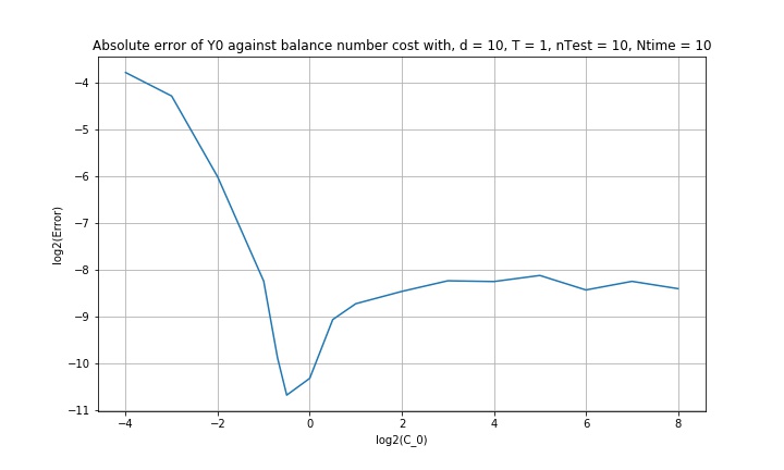
Figure 1: The error of $Y_{0}$ for CN scheme based on the balance number

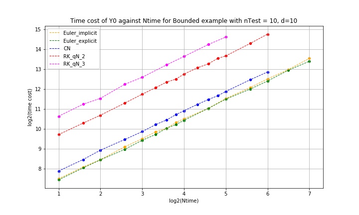
Figure 2: Time cost against time steps for different schemes

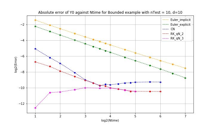
Figure 3: Error against time steps for different schemes

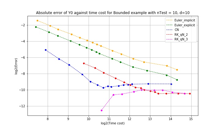
Figure 4: Error against time cost for different schemes

In Figure 4, we compare the convergence rate of the five schemes mentioned above. We verify that the implicit Euler scheme and explicit Euler scheme are almost order 1. The CN scheme is almost order 2. The convergence rate of RK-2 scheme is slightly less than CN scheme, but the error is smaller. The RK-3 scheme converges too fast in terms of discrete time error for us to be able to observe any convergence order.

In Figure 4, we plotted the error w.r.t. the time cost for the five schemes mentioned above. We see that the Euler schemes are slower to reach a small error. The RK-3 scheme has a small error but it is computationally demanding even if the number of time steps $N$ is small. As expected, the CN scheme is faster than RK-2 scheme. In conclusion, if we want an error smaller than $0.01\approx 2^{-6.64}$, CN scheme seems to be the best scheme to use.

4.2 An application with Cox–Ingersoll–Ross process

In this section, we test the Cox–Ingersoll–Ross [13] (CIR for short) process as follows,

$$d\mathcal{X}_{t}=a(b-\mathcal{X}_{t})dt+\sigma\sqrt{\mathcal{X}_{t}}dW_{t},$$

where $\sqrt{\mathcal{X}_{t}}={\rm diag}(\sqrt{\mathcal{X}_{t}^{1}},\cdots,\sqrt{\mathcal{X}_{t}^{d}})$, and with the following conditions to ensure that $(\mathcal{X}_{t})_{t>0}$ is always positive:

$$a>0,\;b>0,\;2ab\geq\sigma^{2},\;\mathcal{X}_{0}\geq 0.$$

We implemented the Ninomiya-Victoir scheme [32]: The weak error is of order $2$, recall (2.19).

We test the BSDE with the same solution of the previous subsection $Y_{t}=u(t,X_{t})=\cos(\bar{X}_{t})e^{\frac{T-t}{2}}$, $Z_{t}^{i}=-\sqrt{\frac{X_{t}^{i}}{d}}\sin(\bar{X}_{t})e^{\frac{T-t}{2}},i=1,\cdots,d$, recalling $\bar{x}:=\sum\limits_{i=1}^{d}x_{i}$, and keep the terminal function $g$ the same with Brownian Motion case, but with the forward diffusion process is CIR process:

$$\mathrm{d}\mathcal{X}_{t} =\frac{1}{5d}(3-\mathcal{X}_{t})\mathrm{d}t+\frac{1}{\sqrt{d}}\sqrt{\mathcal{X}_{t}}\mathrm{d}W_{t},\quad\mathcal{X}_{0}=10\textbf{1}_{d}.$$

Then, we set the driver $f$:

$$\tilde{f}(t,x) =\left(\frac{1}{2}\cos(\bar{x})(1+\frac{\bar{x}}{d})+\sin(\bar{x})(\frac{3}{5}-\frac{\bar{x}}{5d})\right)e^{\frac{T-t}{2}},$$

$$f(t,x,y) =\tilde{f}(t,x)+\frac{1}{5}\left(\sin(\bar{X}_{t})e^{\frac{T-t}{2}}\right)^{2}(y^{2}-\cos(\bar{x})^{2}e^{T-t}),$$

where $\bar{x}=\sum\limits_{i=1}^{d}x_{i}$.

We only compare Crank-Nicolson scheme with implicit Euler scheme in this section. Setting $d=10,T=1,\mathfrak{c}=1$. We test the implicit Euler scheme and Crank-Nicolson scheme with $b=50000$.

In Figure 6 and Figure 6, the implicit Euler scheme is almost order 1, however it can only achieve an error around $2^{-6}$ even $N=256$, which spent more than $2^{18}$ seconds (nearly 5 days). And the Crank-Nicolson scheme is almost order 2, the error can achieve $2^{-10}$ when $N=64$, and the error can be less than $2^{-6}$ with $2^{15}$ seconds (about 9 hours).

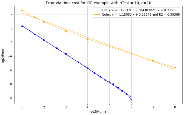
Figure 5: Error against time steps for Euler and CN schemes in CIR case

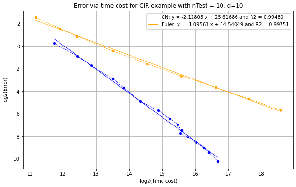
Figure 6: $Y_{0}$ against time steps for for Euler and CN schemes in CIR case

5 Appendix

5.1 Proof of Proposition 2.1

Recalling (2.1)-(2.2) and $\upsilon^{n}_{q}=\mathbb{E}_{t_{n,q}}\!\!\left[|H_{q}^{n}|^{2}\right]$, observe that for $1<q\leq Q+1$, it holds

$$Y_{n,q}=Y_{n+1}+h\sum_{k=1}^{q}a_{qk}f(X_{n,k},Y_{n,k},Z_{n,k})-(Z_{n,q}+A_{n,q})\Delta W_{n,q}+\Delta M_{n,q},$$ (5.1)

where $\mathbb{E}_{t_{n,q}}\!\!\left[\Delta M_{n,q}\right]=\mathbb{E}_{t_{n,q}}\!\!\left[\Delta M_{n,q}\Delta W_{n,q}\right]=0,\mathbb{E}_{t_{n,q}}\!\!\left[|\Delta M_{n,q}|^{2}\right]<\infty$, and

$$A_{n,q} =\mathbb{E}_{t_{n,q}}\!\!\left[H_{q}^{n}\left(Y_{n+1}+h\sum_{k=1}^{q-1}a_{qk}f(X_{n,k},Y_{n,k},Z_{n,k})\right)\right]-Z_{n,q}$$

$$=\mathbb{E}_{t_{n,q}}\!\!\left[\sum_{k=1}^{q-1}\left(a_{qk}H_{q}^{n}-\alpha_{qk}H_{q,k}^{n}\right)hf(X_{n,k},Y_{n,k},Z_{n,k})\right].$$ (5.2)

And for the perturbed scheme defined in (2.14)-(2.15), observe that

$$\tilde{Y}_{n,q}=\tilde{Y}_{n+1}+h\sum_{k=1}^{q}a_{qk}f(X_{n,k},\tilde{Y}_{n,k},\tilde{Z}_{n,k})+\zeta^{y}_{n,q}-(\tilde{Z}_{n,q}+\tilde{A}_{n,q}-\zeta^{z}_{n,q})\Delta W_{n,q}+\Delta\tilde{M}_{n,q},$$ (5.3)

where $\mathbb{E}_{t_{n,q}}\!\!\left[\Delta\tilde{M}_{n,q}\right]=\mathbb{E}_{t_{n,q}}\!\!\left[\Delta\tilde{M}_{n,q}\Delta W_{n,q}\right]=0,\mathbb{E}_{t_{n,q}}\!\!\left[|\Delta\tilde{M}_{n,q}|^{2}\right]<\infty$, and

$$\tilde{A}_{n,q}=\mathbb{E}_{t_{n,q}}\!\!\left[\sum_{k=1}^{q-1}\left(a_{qk}H_{q}^{n}-\alpha_{qk}H_{q,k}^{n}\right)hf(X_{n,k},\tilde{Y}_{n,k},\tilde{Z}_{n,k})\right].$$ (5.4)

Set $\delta Y_{n,q}=Y_{n,q}-\tilde{Y}_{n,q},\delta Z_{n,q}=Z_{n,q}-\tilde{Z}_{n,q},\delta A_{n,q}=A_{n,q}-\tilde{A}_{n,q},\delta f_{n,q}=f(X_{n,q},Y_{n,q},Z_{n,q})-f(X_{n,q},\tilde{Y}_{n,q},\tilde{Z}_{n,q})$, $\delta\Delta M_{n,q}=\Delta M_{n,q}-\Delta\tilde{M}_{n,q}$ for all $0\leq n\leq N-1,1<q\leq Q+1$. From eq. 5.1 and eq. 5.3, we get

$$\delta Y_{n,q}+(\delta Z_{n,q}+\zeta_{n,q}^{z})\Delta W_{n,q}+\delta\Delta M_{n,q}=\delta Y_{n+1}+h\sum_{k=1}^{q}a_{qk}\delta f_{n,k}-\zeta_{n,q}^{y}-\delta A_{n,q}\Delta W_{n,q}.$$ (5.5)

Step 1: For $0\leq n\leq N-1$, control of $\mathbb{E}\!\!\left[|\delta Y_{n}|^{2}\right]$ by the term $h\sum\limits_{k=n}^{N-1}\sum\limits_{q=2}^{Q+1}\mathbb{E}\!\!\left[|\delta Z_{k,q}|^{2}\right]$.
Squaring both sides of (5.5), taking conditional expectation and using Young’s inequality, we obtain

$$|\delta Y_{n,q}|^{2}+c_{q}h|\delta Z_{n,q}+\zeta_{n,q}^{z}|^{2} \leq\left(1+\frac{h}{C}\right)\mathbb{E}_{t_{n,q}}\!\!\left[\left|\delta Y_{n+1}+h\sum_{k=1}^{j}a_{qk}\delta f_{n,k}\right|^{2}\right]$$

$$+2\left(1+\frac{C}{h}\right)\left(\left|\zeta_{n,q}^{y}\right|^{2}+c_{q}h\left|\delta A_{n,q}\right|^{2}\right).$$ (5.6)

Recalling (2.4)-(2.6), and denote $\bar{a}=\max\limits_{q,k}\{|a_{qk}|,|\alpha_{qk}|\}$, thus have

$$\left|\delta A_{n,q}\right|^{2} =h^{2}\left|\mathbb{E}_{t_{n,q}}\!\!\left[\sum\limits_{k=1}^{q-1}(a_{qk}H_{q}^{n}-\alpha_{qk}H_{q,k}^{n})\delta f_{n,k}\right]\right|^{2}$$

$$\leq qh^{2}\sum\limits_{k=1}^{q-1}\mathbb{E}_{t_{n,q}}\!\!\left[|a_{qk}H_{q}^{n}-\alpha_{qk}H_{q,k}^{n}|^{2}\right]\mathbb{E}_{t_{n,q}}\!\!\left[|\delta f_{n,k}|^{2}\right]$$

$$\leq qh^{2}\sum\limits_{k=1}^{q-1}\mathbb{E}_{t_{n,q}}\!\!\left[2a_{qk}^{2}|H_{q}^{n}|^{2}+2\alpha_{qk}^{2}|H_{q,k}^{n}|^{2}\right]\mathbb{E}_{t_{n,q}}\!\!\left[2K^{2}(|\delta Y_{n,k}|^{2}+|\delta Z_{n,k}|^{2})\right]$$

$$\leq 8q^{2}\bar{a}^{2}K^{2}\Lambda h\sum\limits_{k=1}^{q-1}\mathbb{E}_{t_{n,q}}\!\!\left[|\delta Y_{n,k}|^{2}+|\delta Z_{n,k}|^{2}\right]$$

$$\leq Ch\sum\limits_{k=1}^{q-1}\mathbb{E}_{t_{n,q}}\!\!\left[|\delta Y_{n,k}|^{2}+|\delta Z_{n,k}|^{2}\right],$$ (5.7)

and

$$|\delta Z_{n,q}+\zeta_{n,q}^{z}|^{2}\geq(1-\eta)|\delta Z_{n,q}|^{2}+(1-\frac{1}{\eta})|\zeta_{n,q}^{z}|^{2}\geq(1-\eta)|\delta Z_{n,q}|^{2}-\frac{1}{\eta}|\zeta_{n,q}^{z}|^{2},$$ (5.8)

for $\eta>0$. Using the Lipschitz regularity of $f$, Young’s inequality and Jensen’s inequality, for any $\epsilon>0$, we obtain

$$\quad\,\left|\delta Y_{n+1}+h\sum_{k=1}^{q}a_{qk}\delta f_{n,k}\right|^{2}$$

$$\leq\left(|\delta Y_{n+1}|+hK\sum_{k=1}^{q}|a_{qk}|(|\delta Y_{n,k}|+|\delta Z_{n,k}|)\right)^{2}$$

$$\leq\left(\left(1+Ch\right)|\delta Y_{n+1}|+Ch|\delta Z_{n+1}|+Ch\sum_{k=2}^{q}(|\delta Y_{n,k}|+|\delta Z_{n,k}|)\right)^{2}$$

$$\leq\left(1+\frac{h}{\epsilon}\right)\left(\left(1+Ch\right)|\delta Y_{n+1}|^{2}+Ch\sum_{k=2}^{q}|\delta Y_{n,k}|^{2}\right)+C\left(h+\epsilon\right)h\sum_{k=1}^{q}|\delta Z_{n,k}|^{2}.$$

Choosing $h$ small enough and $\epsilon$ such that $C(h+\epsilon)\leq\frac{c_{q}}{2}$, we obtain

$$\left|\delta Y_{n+1}+h\sum_{k=1}^{q}a_{qk}\delta f_{n,k}\right|^{2} \leq\left(1+Ch\right)|\delta Y_{n+1}|^{2}+Ch\sum_{k=2}^{q}|\delta Y_{n,k}|^{2}+\frac{c_{q}h}{2}\sum_{k=1}^{q}|\delta Z_{n,k}|^{2}.$$ (5.9)

Thus choosing $\eta=\frac{1}{4}$ in (5.8), and using (5.9), (5.1) into (5.1), then for $h$ small enough, we get

$$\quad\,|\delta Y_{n,q}|^{2}\leq|\delta Y_{n,q}|^{2}+\frac{c_{q}h}{4}|\delta Z_{n,q}|^{2}$$

$$\leq\left(1+Ch\right)\mathbb{E}_{t_{n,q}}\!\!\left[|\delta Y_{n+1}|^{2}\right]+Ch\sum_{k=1}^{q-1}\mathbb{E}_{t_{n,q}}\!\!\left[|\delta Y_{n,k}|^{2}+|\delta Z_{n,k}|^{2}\right]+\mathbb{E}_{t_{n,q}}\!\!\left[\frac{C}{h}|\zeta_{n,q}^{y}|^{2}+Ch\left|\zeta_{n,q}^{z}\right|^{2}\right]$$

$$\leq\left(1+Ch\right)\mathbb{E}_{t_{n,q}}\!\!\left[|\delta Y_{n+1}|^{2}\right]+Ch\sum_{k=1}^{q-1}\mathbb{E}_{t_{n,q}}\!\!\left[|\delta Z_{n,k}|^{2}\right]+C\sum_{k=2}^{q}\mathbb{E}_{t_{n,q}}\!\!\left[\frac{1}{h}|\zeta_{n,k}^{y}|^{2}+h\left|\zeta_{n,k}^{z}\right|^{2}\right].$$ (5.10)

Using the discrete version of Grönwall’s lemma, we even eventually conclude:

$$\mathbb{E}\!\!\left[|\delta Y_{n}|^{2}\right] \leq C\left(\mathbb{E}\!\!\left[|\delta Y_{N}|^{2}+|\delta Z_{N}|^{2}\right]+h\sum_{k=n}^{N-1}\sum_{q=2}^{Q+1}\mathbb{E}\!\!\left[|\delta Z_{k,q}|^{2}+\frac{1}{h^{2}}|\zeta_{k,q}^{y}|^{2}+\left|\zeta_{k,q}^{z}\right|^{2}\right]\right).$$ (5.11)

Step 2: Control of $h\sum\limits_{k=n}^{N-1}\sum\limits_{q=2}^{Q+1}\mathbb{E}\!\!\left[|\delta Z_{k,q}|^{2}\right]$.
Using the Cauchy-Schwarz inequality and the Lipschitz regularity of $f$, we get

$$h\left|\mathbb{E}_{t_{n,q}}\!\!\left[hH_{q,k}^{n}\delta f_{n,k}\right]\right|^{2} \leq h^{3}\mathbb{E}_{t_{n,q}}\!\!\left[|H_{q,k}^{n}|^{2}\right]\mathbb{E}_{t_{n,q}}\!\!\left[|\delta f_{n,k}|^{2}\right]\leq 2dK^{2}\Lambda h^{2}\mathbb{E}_{t_{n,q}}\!\!\left[|\delta Y_{n,k}|^{2}+|\delta Z_{n,k}|^{2}\right]$$ (5.12)

and

$$\mathbb{E}_{t_{n}}\!\!\left[h\left|\mathbb{E}_{t_{n,q}}\!\!\left[H_{q}^{n}(\delta Y_{n+1}-\mathbb{E}_{t_{n}}\!\!\left[\delta Y_{n+1}\right])\right]\right|^{2}\right] \leq\mathbb{E}_{t_{n}}\!\!\left[h\mathbb{E}_{t_{n,q}}\!\!\left[|H_{q}^{n}|^{2}\right]\mathbb{E}_{t_{n,q}}\!\!\left[|\delta Y_{n+1}-\mathbb{E}_{t_{n}}\!\!\left[\delta Y_{n+1}\right]|^{2}\right]\right]$$

$$\leq\Lambda\mathbb{E}_{t_{n}}\!\!\left[|\delta Y_{n+1}-\mathbb{E}_{t_{n}}\!\!\left[\delta Y_{n+1}\right]|^{2}\right]$$

$$\leq\Lambda\left(\mathbb{E}_{t_{n}}\!\!\left[|\delta Y_{n+1}|^{2}\right]-\mathbb{E}_{t_{n}}\!\!\left[\delta Y_{n+1}\right]^{2}\right).$$ (5.13)

Taking $q=Q+1$ in (5.5), using Young’s inequality, and using the subscript $\{n\}\equiv\{n,Q+1\}$, we get

$$\quad\,\mathbb{E}_{t_{n}}\!\!\left[|\delta Y_{n+1}|^{2}\right]-\mathbb{E}_{t_{n}}\!\!\left[\delta Y_{n+1}\right]^{2}$$

$$=\mathbb{E}_{t_{n}}\!\!\left[|\delta Y_{n+1}|^{2}\right]-\mathbb{E}_{t_{n}}\!\!\left[\delta Y_{n}+\zeta_{n}^{y}-h\sum_{k=1}^{Q+1}a_{qk}\mathbb{E}_{t_{n,q}}\!\!\left[\delta f_{n,k}\right]\right]^{2}$$

$$\leq\mathbb{E}_{t_{n}}\!\!\left[|\delta Y_{n+1}|^{2}\right]-|\delta Y_{n}|^{2}+C\left(|\delta Y_{n}||\zeta_{n}^{y}|+h(|\delta Y_{n}|+|\zeta_{n}^{y}|)\sum_{k=1}^{Q+1}\mathbb{E}_{t_{i}}\!\!\left[|\delta f_{n,k}|\right]\right)$$

$$\leq\mathbb{E}_{t_{n}}\!\!\left[|\delta Y_{n+1}|^{2}\right]-|\delta Y_{n}|^{2}+C\left(|\delta Y_{n}||\zeta_{n}^{y}|+h(|\delta Y_{n}|+|\zeta_{n}^{y}|)\sum_{k=1}^{Q+1}\mathbb{E}_{t_{n,q}}\!\!\left[|\delta Y_{n,k}|+|\delta Z_{n,k}|\right]\right)$$

$$\leq\mathbb{E}_{t_{n}}\!\!\left[|\delta Y_{n+1}|^{2}\right]-|\delta Y_{n}|^{2}+Ch\sum_{k=1}^{Q+1}\mathbb{E}_{t_{n}}\!\!\left[\frac{1}{\epsilon}|\delta Y_{n,k}|^{2}+\epsilon|\delta Z_{n,k}|^{2}\right]+\frac{C}{h}\mathbb{E}_{t_{n}}\!\!\left[|\zeta_{n}^{y}|^{2}\right],$$ (5.14)

for any $\epsilon>0$. Using Jensen’s inequality, and the inequalities (5.12), (5.1), (5.1), we obtain

$$\quad\,h\mathbb{E}_{t_{n}}\!\!\left[|\delta Z_{n,q}|^{2}\right]=h\mathbb{E}_{t_{n}}\!\!\left[\left|\mathbb{E}_{t_{n,q}}\Big{[}H_{q}^{n}\delta Y_{n+1}+h\sum\limits_{k=1}^{q-1}\alpha_{qk}H_{q,k}^{n}\delta f_{n,k}-\zeta_{n,q}^{z}\Big{]}\right|^{2}\right]$$

$$\leq C\mathbb{E}_{t_{n}}\!\!\left[h\left|\mathbb{E}_{t_{n,q}}\!\!\left[H_{q}^{n}(\delta Y_{n+1}-\mathbb{E}_{t_{n}}\!\!\left[\delta Y_{n+1}\right])\right]\right|^{2}+\sum_{k=1}^{q-1}\alpha_{qk}^{2}h\left|\mathbb{E}_{t_{n,q}}\!\!\left[hH_{q,k}^{n}\delta f_{n,k}\right]\right|^{2}+h|\zeta_{n,q}^{z}|^{2}\right]$$

$$\leq C\left(\mathbb{E}_{t_{n}}\!\!\left[|\delta Y_{n+1}|^{2}\right]-|\mathbb{E}_{t_{n}}\!\!\left[\delta Y_{n+1}\right]|^{2}+h^{2}\sum_{k=1}^{q-1}\mathbb{E}_{t_{n}}\!\!\left[|\delta Y_{n,k}|^{2}+|\delta Z_{n,k}|^{2}\right]+h\mathbb{E}_{t_{n}}\!\!\left[|\zeta_{n,q}^{z}|^{2}\right]\right)$$

$$\leq C\left(\mathbb{E}_{t_{n}}\!\!\left[|\delta Y_{n+1}|^{2}\right]-|\delta Y_{n}|^{2}+Ch\sum_{k=1}^{Q+1}\mathbb{E}_{t_{n}}\!\!\left[\frac{1}{\epsilon}|\delta Y_{n,k}|^{2}+\epsilon|\delta Z_{n,k}|^{2}\right]+\mathbb{E}_{t_{n}}\!\!\left[\frac{C}{h}|\zeta_{n}^{y}|^{2}+h|\zeta_{n,q}^{z}|^{2}\right]\right)$$ (5.15)

Summing over $q$ and $n$, setting $\epsilon=\frac{1}{2(Q+2)C}$, and note that the subscript $\{n,1\}\equiv\{n+1\}\equiv\{n+1,Q+1\}$, then for $h$ small enough,

$$\quad\,h\sum_{k=n}^{N-1}\sum_{q=2}^{Q+1}\mathbb{E}\!\!\left[|\delta Z_{k,q}|^{2}\right]$$

$$\leq C\sum_{k=n}^{N-1}\sum_{q=2}^{Q+1}\mathbb{E}\!\!\left[|\delta Y_{k+1}|^{2}-|\delta Y_{k}|^{2}+h\sum_{l=1}^{Q+1}(\frac{1}{\epsilon}|\delta Y_{k,l}|^{2}+\epsilon|\delta Z_{k,l}|^{2})+\frac{1}{h}|\zeta_{k}^{y}|^{2}+h|\zeta_{k,q}^{z}|^{2}\right]$$

$$=C\sum_{k=n}^{N-1}\mathbb{E}\!\!\left[Q|\delta Y_{k+1}|^{2}-Q|\delta Y_{k}|^{2}+\frac{Qh}{\epsilon}\sum_{l=1}^{Q+1}|\delta Y_{k,l}|^{2}+\frac{Q}{h}|\zeta_{k}^{y}|^{2}+h\sum_{q=2}^{Q+1}|\zeta_{k,q}^{z}|^{2}\right]$$

$$\quad+\frac{Qh}{Q+2}\sum_{k=n}^{N-1}\sum_{l=2}^{Q+1}\mathbb{E}\!\!\left[|\delta Z_{k,l}|^{2}\right]$$

so that

$$\quad\,h\sum_{k=n}^{N-1}\sum_{q=2}^{Q+1}\mathbb{E}\!\!\left[|\delta Z_{k,q}|^{2}\right]$$

$$\leq C\sum_{k=n}^{N-1}\mathbb{E}\!\!\left[|\delta Y_{k+1}|^{2}-|\delta Y_{k}|^{2}+h\sum_{q=1}^{Q+1}|\delta Y_{k,q}|^{2}+\frac{1}{h}|\zeta_{k}^{y}|^{2}+h\sum_{q=2}^{Q+1}|\zeta_{k,q}^{z}|^{2}\right]$$

$$\leq C\mathbb{E}\!\!\left[|\delta Y_{N}|^{2}+h|\delta Z_{N}|^{2}+h\sum_{k=n}^{N-1}|\delta Y_{k}|^{2}+\sum_{k=n}^{N-1}\sum_{q=2}^{Q+1}\left(\frac{1}{h}|\zeta_{k,q}^{y}|^{2}+h|\zeta_{k,q}^{z}|^{2}\right)\right]$$ (5.16)

where we used (5.1) and the subscript $\{n,1\}\equiv\{n+1\}\equiv\{n+1,Q+1\},0\leq n\leq N-1$ again in the last line.
Step 3: Control of the term $\mathbb{E}\!\!\left[|\delta Y_{n}|^{2}\right],\;0\leq n\leq N-1$.
Combining the inequality (5.1) with (5.11), we get

$$\mathbb{E}\!\!\left[|\delta Y_{n}|^{2}\right] \leq C\mathbb{E}\!\!\left[|\delta Y_{N}|^{2}+h|\delta Z_{N}|^{2}+h\sum\limits_{k=n}^{N-1}|\delta Y_{k}|^{2}+h\sum_{k=n}^{N-1}\sum_{q=2}^{Q+1}\left(\frac{1}{h^{2}}|\zeta_{k,q}^{y}|^{2}+|\zeta_{k,q}^{z}|^{2}\right)\right].$$ (5.17)

Step 4: Control on $\max\limits_{n\leq k\leq N-1}\mathbb{E}\!\!\left[|\delta Y_{k}|^{2}\right]+h\sum\limits_{k=n}^{N-1}\mathbb{E}\!\!\left[|\delta Z_{k}|^{2}\right]$.
Set $\delta_{n}:=\sum\limits_{k=n}^{N-1}\mathbb{E}\!\!\left[|\delta Y_{k}|^{2}\right]$, and

$$\theta_{n}:=\mathbb{E}\!\!\left[|\delta Y_{N}|^{2}+h|\delta Z_{N}|^{2}\right]+h\sum_{k=n}^{N-1}\sum_{q=2}^{Q+1}\mathbb{E}\!\!\left[\frac{1}{h^{2}}|\zeta_{k,q}^{y}|^{2}+|\zeta_{k,q}^{z}|^{2}\right].$$ (5.18)

It holds

$$\delta_{n}-\delta_{n+1}\leq Ch\delta_{n}+C\theta_{n}.$$ (5.19)

Using the discrete version of Grönwall’s lemma, and noting that $\delta_{N-1}\leq\theta_{n}$, $\theta_{k}\leq\theta_{n}$ for $k\geq n$, we obtain

$$\delta_{n}\leq C\left(\delta_{N-1}+\sum\limits_{k=n}^{N-1}\theta_{k}e^{C(N-k-1)h}\right)\leq C\theta_{n}\frac{1}{e^{Ch}-1}.$$ (5.20)

This last inequality combined with (5.19) leads to

$$\mathbb{E}\!\!\left[|\delta Y_{n}|^{2}\right]=\delta_{n}-\delta_{n+1}\leq C\theta_{n}.$$

For the $Z-$part, the proof is concluded inserting (5.20) into (5.1) with $n=0$ in this equation.

References

- [1] V. Bally and G. Pagès. Error analysis of the optimal quantization algorithm for obstacle problems. Stochastic Processes and their Applications, 106(1):1 – 40, 2003.
- [2] V. Bally and G. Pagès. A quantization algorithm for solving multidimensional discrete-time optimal stopping problems. Bernoulli, 9(6):1003–1049, 2003.
- [3] C. Beck, W. E, and A. Jentzen. Machine learning approximation algorithms for high-dimensional fully nonlinear partial differential equations and second-order backward stochastic differential equations. Journal of Nonlinear Science, pages 1–57, 2017.
- [4] B. Bouchard and N. Touzi. Discrete-time approximation and monte-carlo simulation of backward stochastic differential equations. Stochastic Processes and their Applications, 111(2):175–206, 2004.
- [5] B. Bouchard and T. Touzi. Discrete-time approximation and monte-carlo simulation of backward stochastic differential equations. Stochastic Processes and their Applications, 111(2):175 – 206, 2004.
- [6] P. Briand and C. Labart. Simulation of bsdes by wiener chaos expansion. The Annals of Applied Probability, 24(3):1129–1171, 2014.
- [7] Q. Chan-Wai-Nam, J. Mikael, and X. Warin. Machine learning for semi linear pdes. Journal of Scientific Computing, 79(3):1667–1712, 2019.
- [8] J.-F. Chassagneux. Linear multistep schemes for bsdes. SIAM Journal on Numerical Analysis, 52(6):2815–2836, 2014.
- [9] J.-F. Chassagneux, J. Chen, N. Frikha, and C. Zhou. A learning scheme by sparse grids and picard approximations for semilinear parabolic pdes. arXiv preprint arXiv:2102.12051, 2021.
- [10] J.-F. Chassagneux and D. Crisan. Runge–kutta schemes for backward stochastic differential equations. Annals of Applied Probability, 24(2):679–720, 2014.
- [11] J.-F. Chassagneux and C. Garcia Trillos. Cubature method to solve bsdes: Error expansion and complexity control. Mathematics of Computation, 89(324):1895–1932, 2020.
- [12] J.-F. Chassagneux and M. Yang. Numerical approximation of singular forward-backward sdes. arXiv preprint arXiv:2106.15496, 2021.
- [13] A. Cozma, M. Mariapragassam, and C. Reisinger. Convergence of an euler scheme for a hybrid stochastic-local volatility model with stochastic rates in foreign exchange markets. SIAM Journal on Financial Mathematics, 9(1):127–170, 2018.
- [14] D. Crisan and K. Manolarakis. Solving backward stochastic differential equations using the cubature method: application to nonlinear pricing. SIAM Journal on Financial Mathematics, 3(1):534–571, 2012.
- [15] D. Crisan and K. Manolarakis. Second order discretization of backward sdes and simulation with the cubature method. The Annals of Applied Probability, 24(2):652–678, 2014.
- [16] D. Crisan, K. Manolarakis, and T. Nizar. On the monte carlo simulation of bsdes: An improvement on the malliavin weights. Stochastic Processes and their Applications, 120(7):1133 – 1158, 2010.
- [17] W. E, J. Han, and A. Jentzen. Deep learning-based numerical methods for high-dimensional parabolic partial differential equations and backward stochastic differential equations. Communications in Mathematics and Statistics, 5(4):349–380, 2017.
- [18] M. Germain, H. Pham, and X. Warin. Deep backward multistep schemes for nonlinear pdes and approximation error analysis. arXiv preprint arXiv:2006.01496, 2020.
- [19] M. Germain, H. Pham, and X. Warin. Neural networks-based algorithms for stochastic control and pdes in finance. arXiv preprint arXiv:2101.08068, 2021.
- [20] E. Gobet, J.-P. Lemor, and X. Warin. A regression-based monte carlo method to solve backward stochastic differential equations. The Annals of Applied Probability, 15(3):2172–2202, 2005.
- [21] E. Gobet, J. G. López-Salas, P. Turkedjiev, and C. Vázquez. Stratified regression monte-carlo scheme for semilinear pdes and bsdes with large scale parallelization on gpus. SIAM Journal on Scientific Computing, 38(6):C652–C677, 2016.
- [22] E. Gobet and P. Turkedjiev. Approximation of backward stochastic differential equations using malliavin weights and least-squares regression. Bernoulli, 22(1):530–562, 2016.
- [23] J. Han and J. Long. Convergence of the deep bsde method for coupled fbsdes. Probability, Uncertainty and Quantitative Risk, 5(1):1–33, 2020.
- [24] P. Henry-Labordere, X. Tan, and N. Touzi. A numerical algorithm for a class of bsdes via the branching process. Stochastic Processes and their Applications, 124(2):1112–1140, 2014.
- [25] K. Hornik, M. Stinchcombe, and H. White. Multilayer feedforward networks are universal approximators. Neural networks, 2(5):359–366, 1989.
- [26] Y. Hu, D. Nualart, and X. Song. Malliavin calculus for backward stochastic differential equations and application to numerical solutions. The Annals of Applied Probability, 21(6):2379–2423, 2011.
- [27] C. Huré, H. Pham, and X. Warin. Deep backward schemes for high-dimensional nonlinear pdes. Mathematics of Computation, 89(324):1547–1579, 2020.
- [28] M. Hutzenthaler, A. Jentzen, T. Kruse, et al. On multilevel picard numerical approximations for high-dimensional nonlinear parabolic partial differential equations and high-dimensional nonlinear backward stochastic differential equations. Journal of Scientific Computing, 79(3):1534–1571, 2019.
- [29] Y. Jiang and J. Li. Convergence of the deep bsde method for fbsdes with non-lipschitz coefficients. arXiv preprint arXiv:2101.01869, 2021.
- [30] L. Kapllani and L. Teng. Deep learning algorithms for solving high dimensional nonlinear backward stochastic differential equations. arXiv preprint arXiv:2010.01319, 2020.
- [31] P. E. Kloeden and E. Platen. Stochastic differential equations. In Numerical Solution of Stochastic Differential Equations, pages 103–160. Springer, 1992.
- [32] S. Ninomiya and N. Victoir. Weak approximation of stochastic differential equations and application to derivative pricing. Applied Mathematical Finance, 15(2):107–121, 2008.
- [33] R. E. Nmeir. Quantization-based approximation of reflected bsdes with extended upper bounds for recursive quantization. arXiv preprint arXiv:2105.07684, 2021.
- [34] G. Pagès and A. Sagna. Improved error bounds for quantization based numerical schemes for bsde and nonlinear filtering. Stochastic Processes and their Applications, 128(3):847 – 883, 2018.
- [35] E. Pardoux and S. Peng. Adapted solution of a backward stochastic differential equation. Systems Control Lett., 14(1):55–61, 1990.
- [36] E. Pardoux and S. Peng. Backward stochastic differential equations and quasilinear parabolic partial differential equations. In Stochastic partial differential equations and their applications (Charlotte, NC, 1991), volume 176 of Lect. Notes Control Inf. Sci., pages 200–217. Springer, Berlin, (1992).
- [37] H. Pham, X. Warin, and M. Germain. Neural networks-based backward scheme for fully nonlinear pdes. SN Partial Differential Equations and Applications, 2(1):1–24, 2021.
- [38] A. Takahashi, Y. Tsuchida, and T. Yamada. A new efficient approximation scheme for solving high-dimensional semilinear pdes: control variate method for deep bsde solver. arXiv preprint arXiv:2101.09890, 2021.
- [39] J. Zhang. A numerical scheme for bsdes. The Annals of Applied Probability, 14(1):459–488, 2004.
- [40] W. Zhao, L. Chen, and S. Peng. A new kind of accurate numerical method for backward stochastic differential equations. SIAM Journal on Scientific Computing, 28(4):1563–1581, 2006.
- [41] W. Zhao, G. Zhang, and L. Ju. A stable multistep scheme for solving backward stochastic differential equations. SIAM Journal on Numerical Analysis, 48(4):1369–1394, 2010.