Abstract

The celebrated FedAvg algorithm of McMahan et al. (2017) is based on three components: client sampling (CS), data sampling (DS) and local training (LT). While the first two are reasonably well understood, the third component, whose role is to reduce the number of communication rounds needed to train the model, resisted all attempts at a satisfactory theoretical explanation. Malinovsky et al. (2022) identified four distinct generations of LT methods based on the quality of the provided theoretical communication complexity guarantees. Despite a lot of progress in this area, none of the existing works were able to show that it is theoretically better to employ multiple local gradient-type steps (i.e., to engage in LT) than to rely on a single local gradient-type step only in the important heterogeneous data regime. In a recent breakthrough embodied in their ProxSkip method and its theoretical analysis, Mishchenko et al. (2022) showed that LT indeed leads to provable communication acceleration for arbitrarily heterogeneous data, thus jump-starting the $5^{\rm th}$ generation of LT methods. However, while these latest generation LT methods are compatible with DS, none of them support CS. We resolve this open problem in the affirmative. In order to do so, we had to base our algorithmic development on new algorithmic and theoretical foundations.

1 Introduction

Federated learning (FL) is an emerging paradigm for the training of supervised machine learning models over geographically distributed and often private datasets stored across a potentially very large number of clients’ devices, such as mobile phones, edge devices and hospital servers.

The roots of this young field can be traced to four foundational papers dealing with federated optimization (Konečný et al., 2016a), communication compression (Konečný et al., 2016b), federated averaging (McMahan et al., 2017) and secure aggregation (Bonawitz et al., 2017).

Federated learning has grown massively since its inception—in volume, depth and breadth alike—with many advances in theory, algorithms, systems and practical applications (Kairouz et al., 2019, Li et al., 2020a, Wang et al., 2021).

In this work we study the standard optimization formulation of federated learning, which has the form

$$\textstyle\min\limits_{x\in\mathbb{R}^{d}}\left[f(x)\coloneqq\frac{1}{{M}}\sum\limits_{m=1}^{{M}}f_{m}(x)\right],$$ (1)

where ${M}$ is the number of clients/devices and each function $f_{m}(x)\coloneqq\mathbb{E}_{\xi\sim{\mathcal{D}}_{m}}\!\left[\ell(x,\xi)\right]$ represents the average loss, measured via the loss function $\ell$, of the model parameterized by $x\in\mathbb{R}^{d}$ over the training data ${\mathcal{D}}_{m}$ owned by client $m\in[{M}]\coloneqq\{1,\dots,{M}\}$.

1.1 Federated averaging

Proposed by McMahan et al. (2017), federated averaging (FedAvg) is an immensely popular method specifically designed to solve problem $\left(\ref{eq:main}\right)$ while being mindful of several constraints characteristic of practical federated environments. In particular, FedAvg is based on gradient descent (GD),

but introduces three modifications:

XX a) client sampling (CS),
XX b) data sampling (DS), and
XX c) local training (LT).

Training via FedAvg proceeds in a number of communication rounds. Each round $t$ starts with the selection of a subset/cohort $S^{t}\subseteq[{M}]$ of the clients of size ${C}^{t}=|S^{t}|$; these will participate in the training in this round. The aggregating server then broadcasts the current version of the model, $x^{t}$, to all clients $m\in S^{t}$ in the current cohort. Subsequently, each client $m\in S^{t}$ performs $K$ iterations of SGD on its local loss function $f_{m}$, initiated with $x^{t}$, using minibatches ${\mathcal{B}}_{m}^{k,t}\subseteq{\mathcal{D}}_{m}$ of size $b_{m}=|{\mathcal{B}}_{m}^{k,t}|$ for $k=0,\dots,K-1$. Finally, all participating devices send their updated models to the server for aggregation into a new model $x^{t+1}$, and the process is repeated.

All three modifications can be turned on or off, individually, or in any combination. For example, if we set ${C}^{t}=M$ for all $t$, then all clients are participating in all rounds, i.e., CS is turned off. Further, if we set $b_{m}=|{\mathcal{D}}_{m}|$ for each client $m\in[M]$, then all clients use all their data to compute the local gradient estimator needed to perform each SGD step, i.e., DS is turned off. Finally, if we set $K=1$, then only a single SGD step is taken by each participating client, i.e., LT is turned off. If all of these modifications are turned off, FedAvg reduces to vanilla GD.

1.2 Client and data sampling

While McMahan et al. (2017) provided convincing empirical evidence for the efficacy of FedAvg, their work did not contain any theoretical results. Much progress in FL in the last five years can be attributed to the efforts by the FL community to understand, analyze, and improve upon these mechanisms, often first in isolation, as this is easier when deep understanding is desired.

Since unbiased client and data sampling mechanisms are intimately linked to the stochastic approximation literature dating back to the work of Robbins and Monro (1951), it is not surprising that CS and DS are relatively well understood. For example, variants of SGD supporting virtually arbitrary unbiased CS and DS mechanisms have been analyzed by Gower et al. (2019a) in the smooth strongly convex regime and by Khaled and Richtárik (2020), Chen et al. (2022) in the smooth nonconvex regime. Oracle optimal (in the smooth nonconvex regime) variants of SGD supporting virtually arbitrary unbiased CS and DS mechanisms were proposed and analyzed by Tyurin et al. (2022), who built upon the previous works of Li et al. (2021), Fang et al. (2018) and Nguyen et al. (2017).

However, all the works mentioned above analyze GD + CS/DS only, with LT turned off. If LT is included in the mix as well, or even considered in isolation as a single add-on to vanilla GD, significant technical issues arise. These issues have kept the FL community uneasy and therefore busy and immensely productive for many years. Since, as we shall see, this will be of crucial importance for us to motivate the contributions of this paper, we will now outline the development of the theoretical understanding of the LT mechanism by the FL community over the last seven years.

1.3 Local training

Local training—the practice of requiring each participating client to perform multiple local optimization steps (as opposed to performing a single step only) based on their local data before communication-expensive parameter synchronization is allowed to take place—is one of the most practically useful algorithmic ingredients in the training of FL models. In fact, LT is so central to the practical success of FL, and so unique and novel within the trio (CS, DS and LT) of techniques forming the FedAvg method, that many authors attach the prefix “Fed” (meaning “federated”) to any optimization method performing some version of LT, whether CS and DS are present as well or not.

While LT was popularized by McMahan et al. (2017), it was proposed in the same form before (Povey et al., 2015, Moritz et al., 2016), also without any theoretical justification. However, until recently, the empirically observed and often very significant communication-saving potential of LT remained elusive, escaping all attempts at a satisfying theoretical justification.

1.4 Five generations of local training methods

We shall now briefly review the development of the theoretical understanding of LT in the smooth strongly convex regime. We follow the classification proposed by Malinovsky et al. (2022), who identified five distinct generations of LT methods—1) heuristic, 2) homogeneous, 3) sublinear, 4) linear, and 5) accelerated—each new improving upon the previous one in a certain important way.

1^st generation of LT methods (heuristic). The 1^st generation methods offer ample empirical evidence, but do not come with any convergence rates (Povey et al., 2015, Moritz et al., 2016, McMahan et al., 2017).

2^nd generation of LT methods (homogeneous). The 2^nd generation LT methods do provide guarantees, but their analysis crucially depends on one or another of the many incarnations of data homogeneity assumptions, such as i) bounded gradients, i.e., requiring $\|\nabla f_{m}(x)\|\leq c$ for all $m\in[{M}]$ and $x\in\mathbb{R}^{d}$ (Li et al., 2020b), or ii) bounded gradient dissimilarity (a.k.a. strong growth), i.e., requiring $\frac{1}{{M}}\sum_{m=1}^{M}\|\nabla f_{m}(x)\|^{2}\leq c\|\nabla f(x)\|^{2}$ for all $x\in\mathbb{R}^{d}$ (Haddadpour and Mahdavi, 2019). This is problematic since such assumptions are prohibitively restrictive; indeed, they are typically not satisfied in real FL environments (Kairouz et al., 2019, Wang et al., 2021).

3^rd generation of LT methods (sublinear). The 3^rd generation LT theory managed to succeed in disposing of the problematic data homogeneity assumptions (Khaled et al., 2019, 2020). Woodworth et al. (2020) and Glasgow et al. (2022) subsequently provided lower bounds for LocalGD with DS, showing that its communication complexity is not better than that of minibatch SGD in the heterogeneous data setting. Additionally, Malinovsky et al. (2020) analyzed LT methods for general fixed point problems.

Unfortunately, these results suggest that LT-enhanced GD, often called LocalGD, suffers from a sublinear convergence rate, which is clearly inferior to the linear convergence rate of vanilla GD. While removing the reliance on data homogeneity assumptions was clearly an important step forward, this rather pessimistic theoretical result seems to suggest that LT makes GD worse. However, this is at odds with the empirical evidence, which maintains that LT enhances GD, and often significantly so. For these reasons, theoreticians continued to soldier on, with the quest to at least close the theoretical gap between LT-based methods and vanilla GD.

4^th generation of LT methods (linear). These efforts led to the identification of the client drift phenomenon as the culprit responsible for the gap, and to a solution based on various techniques for the reduction of client drift. This development marks the start of the 4^th generation of LT methods. The first method belonging to this generation, called Scaffold, and due to Karimireddy et al. (2020), employs a SAGA-like variance reduction technique (Defazio et al., 2014) to tame the client drift caused by LT. As a result, Scaffold has the same communication complexity as GD. Gorbunov et al. (2021) subsequently proposed a unified framework for designing and analyzing 3^rd and 4^th generation in a single theorem, including new 4^th generation LT methods such S-Local-GD and S-Local-SVRG. Finally, Mitra et al. (2021) proposed the FedLin method, which can be seen as a variant of one of the methods from Gorbunov et al. (2021) allowing for the clients to take different number of local steps (without this leading to any theoretical benefit).

5^th generation of LT methods (accelerated). In a recent breakthrough, Mishchenko et al. (2022) proved that a certain new and simple form of local training, embodied in their ProxSkip method, leads to provable communication acceleration in the smooth strongly convex regime, even in the notoriously difficult heterogeneous data setting in which the client data $\{{\mathcal{D}}_{m}\}_{m=1}^{{M}}$ is allowed to be arbitrarily different. In particular, if each $f_{m}$ is $L$-smooth and $\mu$-strongly convex, then ProxSkip solves $\left(\ref{eq:main}\right)$ in ${\mathcal{O}}(\sqrt{\nicefrac{{L}}{{\mu}}}\log\nicefrac{{1}}{{\varepsilon}})$ communication rounds, which is a significant acceleration when compared with the ${\mathcal{O}}(\nicefrac{{L}}{{\mu}}\log\nicefrac{{1}}{{\varepsilon}})$ complexity of GD. According to Scaman et al. (2019), this accelerated communication complexity is optimal. Mishchenko et al. (2022) provided several extensions of their method. In particular, ProxSkip was enhanced with a very flexible DS mechanism which can capture virtually any form of (unbiased and non-variance-reduced) data sampling scheme. Motivated by this progress, several other methods belonging to the 5^th generation of LT methods were recently proposed.

First, Malinovsky et al. (2022) extended the ProxSkip method via the inclusion of virtually arbitrary variance-reduced SGD methods (Gorbunov et al., 2020) in lieu of simple SGD, inlcuding SVRG (Johnson and Zhang, 2013, Konečný and Richtárik, 2017), SAGA (Defazio et al., 2014), JacSketch (Gower et al., 2020), L-SVRG (Hofmann et al., 2015, Kovalev et al., 2020a) or DIANA (Mishchenko et al., 2019, Horváth et al., 2019).

Second, Condat and Richtárik (2022) observed that the Bernoulli-type randomness employed in the ProxSkip method whose role is to avoid the computation of an expensive proximity operator is a special case of a more general principle: the application of an unbiased compressor to the proximity operator, combined with a bespoke variance reduction mechanism to tame the variance introduced by the compressor. Condat and Richtárik (2022) further generalized the forward-backward setting used by Mishchenko et al. (2022) to more complex splitting schemes involving the sum of three operators (e.g., ADMM (Hestenes, 1969, Powell, 1969) and PDDY (Davis and Yin, 2017, Salim et al., 2022)), and besides analyzing the smooth strongly convex regime, provided results in the convex regime as well.

Finally, Sadiev et al. (2022) pioneered an alternative approach, based on an LT-friendly modification of the celebrated Chambolle-Pock method (Chambolle and Pock, 2011). In their APDA-Inexact method, the accelerated communication complexity is preserved, but compared to ProxSkip, the # of gradient-type LT steps in each communication round is improved from ${\mathcal{O}}(\kappa^{1/2})$ to ${\mathcal{O}}(\kappa^{1/3})$ and ${\mathcal{O}}(\kappa^{1/4})$, where $\kappa=\nicefrac{{L}}{{\mu}}$ is the condition number. They further improve on some results of Mishchenko et al. (2022) related to the decentralized regime where communication happens along the edges of a connected network.

2 Contributions

Table 1: Comparison of all 5^th generation local training (LT) methods. Our 5GCS method is the first that supports client sampling (CS). Moreover, similarly to APDA-Inexact, our theory allows for the LT solver to be chosen virtually arbitrarily.

5th generation LT Method	LT Solver	Data Sampling	Client Sampling	Reference
ProxSkip	GD, SGD	✓(a)	✗	Mishchenko et al. (2022)
ProxSkip-VR	GD, SGD, VR-SGD	✓(b)	✗	Malinovsky et al. (2022)
APDA-Inexact	any	✗	✗	Sadiev et al. (2022)
RandProx	GD	✗	✗	Condat and Richtárik (2022)
5GCS	any	✓	✓	this work

• Only supports non-variance reduced DS on clients.

• Supports non-variance reduced and variance-reduced DS on clients.

Now that the FL community finally managed to show that (appropriately designed) LT techniques, which as we have seen are key behind the success of modern federated optimization methods for solving $\left(\ref{eq:main}\right)$, lead to provable communication acceleration guarantees (in the smooth strongly convex regime), we adopt the stance that further algorithmic and theoretical progress in FL should be focused on advancing the 5^th generation of LT methods.

To the best of our knowledge, there are only a handful of papers providing methods and results that belong to this latest generation of LT methods (Mishchenko et al., 2022, Malinovsky et al., 2022, Sadiev et al., 2022, Condat and Richtárik, 2022). A close examination of these works reveals that much is yet to be discovered.

2.1 The open problem we address in this work

The starting point of our work is the observation that none of the 5^th generation local training (LT) methods support client sampling (CS). In other words, it is not known whether it is possible to design a method that would enjoy communication acceleration via LT and at the same time also support CS.

The problem is harder than one may initially think. We have talked to several people about this, including the authors of the ProxSkip method. It turns out that they have tried—“very hard” in their own words—but their efforts did not bear any fruit. We have tried as well, and failed. The analysis of ProxSkip is remarkably tight, and every adaptation towards supporting CS seems to either lead to technical problems during the proof construction, or to a loss of communication acceleration. In fact, it is not even clear how should a CS variant of ProxSkip look like. Our attempts at guessing what such a method could look like failed as well, and the variants we brainstormed diverged in our numerical experiments as soon as CS was enabled.

Fortunately, it turns out that these negative results were helpful to us after all. Indeed, they led us to the idea that we should try to develop an entirely different method; one that is not based on either ProxSkip nor APDA-Inexact. Once we started to think outside the box created by our pre-conceived solution path, we eventually managed to succeed.

2.2 Summary of contributions

Table 2: Variants of 5GCS (Algorithm 1) depending on the choice of the LT procedure run by clients $m\in S^{t}$ in the current cohort. ${M}=$ number of clients; ${C}=$ cohort size.

Algorithm	Local Training via Subroutine ${\mathcal{A}}$	Communication Complexity	Theorem
5GCS∞ (a)	$K=\infty$ steps of GD	${\mathcal{O}}\left(\left(\frac{{M}}{{C}}+\sqrt{\frac{{M}}{{C}}\frac{L}{\mu}}\right)\log\frac{1}{\varepsilon}\right)$	3.1
5GCSK	$K={\mathcal{O}}(\sqrt{\frac{{C}}{{M}}\frac{L}{\mu}})$ steps of GD	${\mathcal{O}}\left(\left(\frac{{M}}{{C}}+\sqrt{\frac{{M}}{{C}}\frac{L}{\mu}}\right)\log\frac{1}{\varepsilon}\right)$	3.3
5GCS0 (b)	$K=0$ steps of GD	${\mathcal{O}}\left(\frac{{M}}{{C}}\frac{L}{\mu}\log\frac{1}{\varepsilon}\right)$ (c)	3.5
5GCSA	any method ${\mathcal{A}}$ (as long as it satisfies Assumption 2)	${\mathcal{O}}\left(\left(\frac{{M}}{{C}}+\sqrt{\frac{{M}}{{C}}\frac{L}{\mu}}\right)\log\frac{1}{\varepsilon}\right)$	3.7

• This method can be found in the appendix as Algorithm 2.

• This method can be found in the appendix as Algorithm 3.

• Does not have accelerated communication complexity. Indeed, the communication complexity is ${\mathcal{O}}\left(\nicefrac{{L}}{{\mu}}\log\nicefrac{{1}}{{\varepsilon}}\right)$ instead of ${\mathcal{O}}\left(\sqrt{\nicefrac{{L}}{{\mu}}}\log\nicefrac{{1}}{{\varepsilon}}\right)$ in the ${C}={M}$ regime.

We are now ready to outline the key insights and contributions of our work. Our main idea is to start our development with the remarkable Point-SAGA method of Defazio (2016). The key appealing property of this method is that it can solve $\left(\ref{eq:main}\right)$ with an accelerated rate in the smooth strongly convex regime. However, Point-SAGA has two critical drawbacks:

X (i) In each communication round, Point-SAGA samples a single client only, uniformly at random, which means it supports a very rudimentary and hence not practically interesting form of CS only.

X (ii) Point-SAGA requires a prox-oracle for each $f_{m}$, where $m$ is the active client, i.e.,

$$\textstyle\mathrm{prox}_{\frac{1}{\tau}f_{m}}(x)\coloneqq\arg\min\limits_{u\in\mathbb{R}^{d}}\left\{f_{m}(u)+\frac{\tau}{2}\|x-u\|^{2}\right\}$$

for some $x\in\mathbb{R}^{d}$ and $\tau>0$ in each communication round, and do it exactly. This is problematic, since exact evaluation of the proximity operator is rarely possible, and inexact evaluation (with a small error) may be overly expensive, imparting an excessive computational burden on the clients.

Our main contributions can be summarized as follows.

$\diamond$ We propose a new LT method for FL, which we call 5GCS (Algorithm 1), which achieves accelerated communication complexity, and also supports client sampling. To the best of our knowledge, this is the first 5^th generation LT method which works with client sampling (see Table 1). Moreover, according to Woodworth and Srebro (2016), the communication complexity of 5GCS is optimal.

$\diamond$ Our method supports arbitrary LT subroutines as long as they satisfy a certain technical assumption (Assumption 2). See Table 2 for a list of four variants of 5GCS depending on what LT subroutine is applied, and the associated communication complexities.

$\diamond$ When an infinity of GD steps is used as the LT subroutine, our method 5GCS in each communication round evaluates the prox of $f_{m}$ for all clients $m$ in the cohort, and reduces to a minibatch version of PointSAGA, which is new. While this method enjoys accelerated communication complexity, its reliance on a prox oracle puts a heavy computation burden on the clients. On the other hand, when zero GD steps are used as a subroutine, our method achieves linear but nonaccelerated communication complexity only. Fortunately, it is sufficient to apply a relatively small number of GD steps as the LT subroutine while preserving the accelerated communication complexity of minibatch PointSAGA.

$\diamond$ Several further contributions are mentioned in the remaining text.

3 Main Results

Algorithm 1 5GCS

1:  Input: initial primal iterates $x^{0}\in\mathbb{R}^{d}$; initial dual iterates $u_{1}^{0},\dots,u_{{M}}^{0}\in\mathbb{R}^{d}$; primal stepsize ${\gamma}>0$; dual stepsize ${\tau}>0$; cohort size ${C}\in\{1,\dots,{M}\}$

2:  Initialization: $v^{0}\coloneqq\sum_{m=1}^{M}u_{m}^{0}$ $\diamond$ The server initiates $v^{0}$ as the sum of the initial dual iterates

3:  for communication round $t=0,1,\ldots$ do

4:     Choose a cohort $S^{t}\subset\{1,\ldots,{M}\}$ of clients of cardinality ${C}$, uniformly at random $\diamond$ CS step

5:     Compute $\hat{x}^{t}=\frac{1}{1+{\gamma}\mu}\left(x^{t}-{\gamma}v^{t}\right)$ and broadcast it to the clients in the cohort

6:     for $m\in S^{t}$ do

7:        Find $y_{m}^{K,t}$ as the final point after $K$ iterations of some local optimization algorithm $\mathcal{A}_{m}$, initiated with $y_{m}^{0}=\hat{x}^{t}$, for solving the optimization problem $\diamond$ Client $m$ performs $K$ LT steps

$$\textstyle y_{m}^{K,t}\approx\operatorname*{arg\,min}\limits_{y\in\mathbb{R}^{d}}\left\{\psi^{t}_{m}(y)\coloneqq F_{m}(y)+\frac{{\tau}}{2}\left\|y-\left(\hat{x}^{t}+\frac{1}{{\tau}}u_{m}^{t}\right)\right\|^{2}\right\}$$ (2)

8:        Compute $u_{m}^{t+1}=\nabla F_{m}(y_{m}^{K,t})$ and send it to the server $\diamond$ Client $m$ updates its dual iterate

9:     end for

10:     for $m\in\{1,\ldots,{M}\}\backslash S^{t}$ do

11:        $u_{m}^{t+1}\coloneqq u_{m}^{t}$ $\diamond$ Non-participating clients do nothing

12:     end for

13:     $v^{t+1}\coloneqq\sum_{m=1}^{{M}}u_{m}^{t+1}$ $\diamond$ The server maintains $v^{t+1}$ as the sum of the dual iterates

14:     $x^{t+1}\coloneqq\hat{x}^{t}-{\gamma}\frac{{M}}{{C}}(v^{t+1}-v^{t})$ $\diamond$ The server updates the primal iterate

15:  end for

In this section we describe our new method, 5GCS (Algorithm 1) for solving $\left(\ref{eq:main}\right)$, and formulate our main convergence results (see Table 2 for a summary).

3.1 Convexity and smoothness

In our analysis we focus on the regime when each $f_{m}$ is $L$-smooth and $\mu$-strongly convex, which are standard assumptions in the convex optimization literature.

Assumption 1.

The functions $f_{m}$ are $L$-smooth and $\mu$-strongly convex for all $m\in\{1,\dots,{M}\}$.

We shall use this assumption in what follows without explicitly mentioning this. Recall that a continuously differentiable function $\phi:\mathbb{R}^{d}\to\mathbb{R}$ is $L$-smooth if $\phi(x)-\phi(y)-\langle\nabla\phi(y),x-y\rangle\leq\frac{L}{2}\|x-y\|^{2}$ for all $x,y\in\mathbb{R}^{d}$, and $\mu$-strongly convex if $\phi(x)-\phi(y)-\langle\nabla\phi(y),x-y\rangle\geq\frac{\mu}{2}\|x-y\|^{2}$ for all $x,y\in\mathbb{R}^{d}$.

3.2 Problem reformulation and its dual

Our method applies to a certain reformulation of $\left(\ref{eq:main}\right)$ which we shall now describe. Let ${{H}}\colon\mathbb{R}^{d}\to\mathbb{R}^{{M}d}$ be the linear operator which maps $x\in\mathbb{R}^{d}$ into the vector $(x,\dots,x)\in\mathbb{R}^{{M}d}$ consisting of ${M}$ copies of $x$. First, notice that $F_{m}(x)\coloneqq\frac{1}{{M}}(f_{m}(x)-\frac{\mu}{2}\left\|x\right\|^{2})$ is convex and $L_{F}$-smooth with $L_{F}\coloneqq\frac{1}{{M}}(L-\mu)$. Further, define $F:\mathbb{R}^{{M}d}\to\mathbb{R}$ via $F(x_{1},\dots,x_{M})\coloneqq\sum_{m=1}^{{M}}F_{m}(x_{m}).$

Having established the necessary notation, we consider the following reformulation of problem $\left(\ref{eq:main}\right)$:

$$\textstyle x^{\star}=\operatorname*{arg\,min}\limits_{x\in\mathbb{R}^{d}}\left[f(x)\coloneqq F({{H}}x)+\frac{\mu}{2}\left\|x\right\|^{2}\right].$$ (3)

It is straightforward to see that $f$ from $\left(\ref{eq:main}\right)$ and $\left(\ref{eq:main-new}\right)$ are identical functions. The dual problem to $\left(\ref{eq:main-new}\right)$ is

$$\textstyle u^{\star}=\operatorname*{arg\,max}\limits_{u\in\mathbb{R}^{{M}d}}\,\left(\frac{1}{2\mu}\left\|\sum\limits_{m=1}^{{M}}u_{m}\right\|^{2}+\sum\limits_{m=1}^{{M}}F_{m}^{*}(u_{m})\right),$$

where $F_{m}^{*}$ is the Fenchel conjugate of $F_{m}$, defined by $F_{m}^{*}(y)\coloneqq\sup_{x\in\mathbb{R}^{d}}\{\langle x,y\rangle-F_{m}(x)\}.$ Under Assumption 1, the primal and dual problems have unique optimal solutions $x^{\star}$ and $u^{\star}$, respectively.

3.3 The 5GCS algorithm

Our proposed algorithm, 5GCS, is formalized as Algorithm 1. The method produces a sequence of primal iterates $x^{t}$, and a sequence of dual iterates $u^{t}=(u_{1}^{t},\dots,u_{M}^{t})$. We have added several comments explaining the steps, and believe that the method should be easy to parse without additional commentary. In each communication round $t$, the participating clients $m\in S^{t}$ in parallel perform LT via $K$ steps of GD applied to minimizing function $\psi^{t}_{m}$; see $\left(\ref{localprob}\right)$. Below we outline four special variants of 5GCS, depending on the choice of the LT subroutines $\{{\mathcal{A}}_{m}\}_{m=1}^{{M}}$.

3.4 LT subroutine: GD with $K=+\infty$ steps (i.e., prox)

The choice $K=+\infty$ corresponds to exact minimization of function $\psi^{t}_{m}$ defined in $\left(\ref{localprob}\right)$, i.e., to the evaluation of the prox operator of $F_{m}$ for all $m\in S^{t}$. In this case, 5GCS reduces to Minibatch-Point-SAGA (see Algorithm 2), and its convergence properties are described by the next result.

Theorem 3.1.

Consider Algorithm 1 (5GCS) with the LT solver being GD run for $K=+\infty$ iterations (this is equivalent to Algorithm 2; we shall also call the method 5GCS_∞). Let ${\gamma}>0$, ${\tau}>0$ and ${\gamma}{\tau}\leq\frac{1}{{M}}$. Then for the Lyapunov function

$$\textstyle\Psi^{t}\coloneqq\frac{1}{{\gamma}}\left\|x^{t}-x^{\star}\right\|^{2}+\frac{{M}}{{C}}\left(\frac{1}{{\tau}}+2\frac{1}{L_{F}}\right)\left\|u^{t}-u^{\star}\right\|^{2},$$

the iterates of the method satisfy $\mathbb{E}\!\left[\Psi^{T}\right]\leq(1-\rho)^{T}\Psi^{0},$ where $\rho\coloneqq\min\left(\frac{{\gamma}\mu}{1+{\gamma}\mu},\frac{{C}}{{M}}\frac{2{\tau}}{L_{F}+2{\tau}}\right)<1.$

The following corollary gives a bound on the number of communication rounds needed to solve the problem.

Corollary 3.2.

Choose any $0<\varepsilon<1$. If we choose ${\gamma}=\sqrt{\frac{2{C}}{L_{F}\mu{M}^{2}}}$ and ${\tau}=\sqrt{\frac{L_{F}\mu}{2{C}}}$, then in order to guarantee $\mathbb{E}\!\left[\Psi^{T}\right]\leq\varepsilon\Psi^{0}$, it suffices to take

$$\textstyle T\geq\left(\frac{{M}}{{C}}+\sqrt{\frac{{M}}{{C}}\frac{L-\mu}{2\mu}}\right)\log\frac{1}{\varepsilon}=\tilde{{\mathcal{O}}}\left(\frac{{M}}{{C}}+\sqrt{\frac{{M}}{{C}}\frac{L}{\mu}}\right)$$

communication rounds.

Note that the communication complexity improves as the cohort size ${C}$ increases, and becomes $\tilde{{\mathcal{O}}}(\sqrt{\nicefrac{{L}}{{\mu}}})$ for ${C}={M}$. This recovers the accelerated communication complexity of existing 5^th generation local training (LT) methods ProxSkip, ProxSkip-VR and APDA-Inexact in the regime when GD is used as the LT method. However, unlike these methods, 5GCS_∞ supports client sampling (CS). In the opposite extreme, i.e., when the cohort size is minimal (${C}=1$), the communication complexity of 5GCS_∞ becomes $\tilde{{\mathcal{O}}}({M}+\sqrt{\nicefrac{{{M}L}}{{\mu}}})$. If $\nicefrac{{L}}{{\mu}}\leq{M}$, which will typically be the case in FL settings with a very large number of clients (e.g., cross-device FL), the complexity simplifies to $\tilde{{\mathcal{O}}}({M})$, which says that we need as many communication rounds as there are clients, which makes sense, since we do not assume any form of data homogeneity, and this means that all clients may contain valuable data. In general, as the cohort size ${C}$ increases, the communication complexity improves, and interpolates between these two extreme cases.

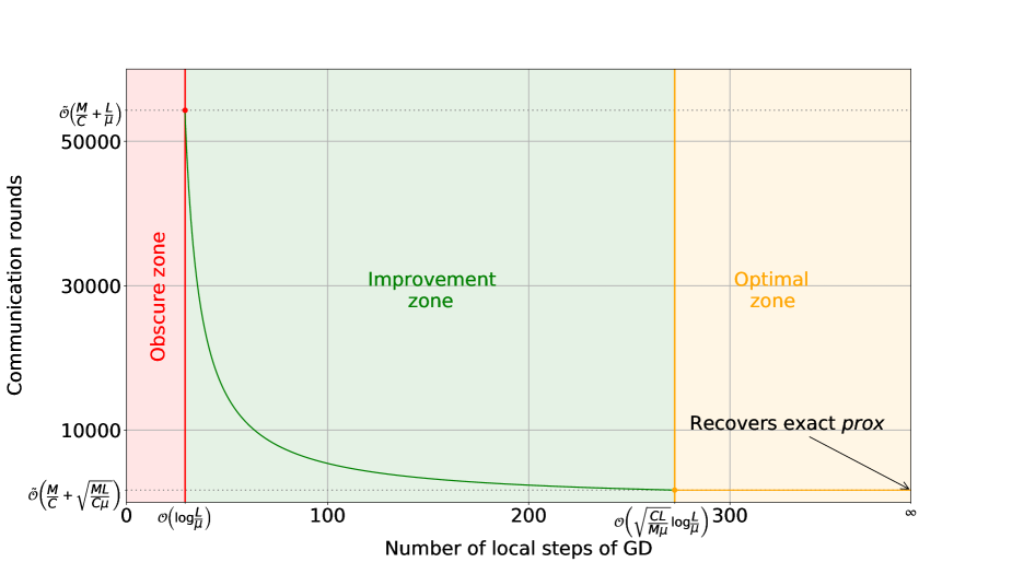
Figure 1: The number of communication rounds of 5GCS as a function of the number of GD steps forming the LT subroutine ${\mathcal{A}}$ with $\nicefrac{{L}}{{\mu}}=10^{4}$ and $\nicefrac{{{C}}}{{{M}}}=0.1$. The key observation is that it is enough to choose $K={\mathcal{O}}(\sqrt{\frac{{M}}{{C}}\frac{L}{\mu}})$, which is at the left end-point of the “optimal zone”. More steps do not lead to better communication complexity.

3.5 LT subroutine: GD with $K={\mathcal{O}}(\sqrt{\frac{{C}}{{M}}\frac{L}{\mu}})$ steps

The key drawback of 5GCS_∞ is that the LT subroutine needs to take an infinite number of GD steps, or equivalently, the method requires the exact evaluation of the prox of $F_{m}$. We now show that it is possible to obtain the same accelerated communication complexity as in the $K=+\infty$ case with a finite, and in fact surprisingly small, number of GD iterations.

Theorem 3.3.

Consider Algorithm 1 (5GCS) with the LT solver being GD run for $K\geq\left(\frac{3}{4}\sqrt{\frac{{C}}{{M}}\frac{L}{\mu}}+2\right)\log\left(4\frac{L}{\mu}\right)$ iterations. Let $0<{\gamma}\leq\frac{3}{16}\sqrt{\frac{{C}}{L\mu{M}}}$ and ${\tau}=\frac{1}{2{\gamma}{M}}$. Then for the Lyapunov function

$$\textstyle\Psi^{t}\coloneqq\frac{1}{{\gamma}}\left\|x^{t}-x^{\star}\right\|^{2}+\frac{{M}}{{C}}\left(\frac{1}{{\tau}}+\frac{1}{L_{F}}\right)\left\|u^{t}-u^{\star}\right\|^{2},$$

the iterates of the method satisfy $\mathbb{E}\!\left[\Psi^{T}\right]\leq(1-\rho)^{T}\Psi^{0},$ where $\rho\coloneqq\min\left\{\frac{{\gamma}\mu}{1+{\gamma}\mu},\frac{{C}}{{M}}\frac{{\tau}}{(L_{F}+{\tau})}\right\}<1.$

Note that GD needs to be run for $K={\mathcal{O}}\left(\sqrt{\frac{{C}}{{M}}\frac{L}{\mu}}\right)$ local steps on each client in the cohort. This quantity depends on the square root of the condition number only, and is smaller for smaller cohort size ${C}$.

It turns out that this result can be improved using a finer analysis. In particular, we can show that some clients can get away with fewer LT steps than this, provided that their local datasets are favorable. To see this, assume that each $f_{m}$ is $L_{m}$-smooth. Clearly, this implies that each $f_{m}$ is $L$-smooth with $L=\max_{m}L_{m}$, and Theorem 3.3 holds with this $L$. However, recall that client $m$ applies GD to (approximately) minimize $\psi^{t}_{m}$ from $\left(\ref{localprob}\right)$, and this function happens to be $\left(\frac{1}{{M}}\left(L_{m}-\mu\right)+{\tau}\right)$-smooth and ${\tau}$-strongly convex. It can be easily seen that ${\tau}\geq\frac{8}{3}\sqrt{\frac{\mu L}{{M}{C}}}$, and hence the condition number of $\psi^{t}_{m}$ is $\frac{1}{{M}}\left(L_{m}-\mu\right)\frac{1}{{\tau}}+1\leq\frac{3}{8}\sqrt{\frac{{C}}{{M}}\frac{\nicefrac{{L_{m}^{2}}}{{L}}}{\mu}}+1$. So, GD only needs $K_{m}={\mathcal{O}}\left(\sqrt{\frac{{C}}{{M}}\frac{\nicefrac{{L_{m}^{2}}}{{L}}}{\mu}}\right)$ iterations on client $m$, which can be much smaller than the worst-case bound $K={\mathcal{O}}\left(\sqrt{\frac{{C}}{{M}}\frac{L}{\mu}}\right)$.

The following corollary gives a bound on the number of communication rounds needed to solve the problem.

Corollary 3.4.

Choose any $0<\varepsilon<1$ and ${\gamma}=\frac{3}{16}\sqrt{\frac{{C}}{L\mu{M}}}$. In order to guarantee $\mathbb{E}\!\left[\Psi^{T}\right]\leq\varepsilon\Psi^{0}$, it suffices to take

$$\textstyle T \geq \textstyle\max\left\{1+\frac{16}{3}\sqrt{\frac{{M}}{{C}}\frac{L}{\mu}},\frac{{M}}{{C}}+\frac{3}{8}\sqrt{\frac{{M}}{{C}}\frac{L}{\mu}}\right\}\log\frac{1}{\varepsilon}$$

$$= \textstyle\tilde{{\mathcal{O}}}\left(\frac{{M}}{{C}}+\sqrt{\frac{{M}}{{C}}\frac{L}{\mu}}\right)$$

communication rounds.

This is the same expression as that from Corollary 3.2, and hence the same comments we’ve made there apply here, too.

3.6 LT subroutine: GD with $K=0$ steps

Theorem 3.5.

Consider Algorithm 1 (5GCS) with the LT solver being GD run for $K=0$ iterations (this is equivalent to Algorithm 3; we shall also call the method 5GCS₀). Let $0<{\gamma}\leq\frac{{C}}{4L{M}}$. Then for the Lyapunov function

$$\textstyle\Psi^{t}\coloneqq\frac{{C}}{{M}^{2}{\gamma}^{2}}\left(1-\sqrt{\frac{{\gamma}{M}L_{F}}{2}}\right)\left\|x^{t}-x^{\star}\right\|^{2}+\left\|u^{t}-u^{\star}\right\|^{2},$$

the iterates of the method satisfy $\mathbb{E}\!\left[\Psi^{T}\right]\leq\left(1-\rho\right)^{T}\Psi^{0},$ where $\rho\coloneqq\min\left(\frac{{\gamma}\mu}{1+{\gamma}\mu},\frac{{C}}{{M}+2{\gamma}L_{F}{M}^{2}}\right)<1.$

The following corollary gives a bound on the number of communication rounds needed to solve the problem.

Corollary 3.6.

Choose any $0<\varepsilon<1$ and ${\gamma}=\frac{{C}}{4L{M}}$. In order to guarantee $\mathbb{E}\!\left[\Psi^{T}\right]\leq\varepsilon\Psi^{0}$, it suffices to take

$$\textstyle T\geq\max\left\{1+\frac{4{M}}{{C}}\frac{L}{\mu},\frac{{M}}{{C}}+\frac{L_{F}{M}}{L}\right\}\log\frac{1}{\varepsilon}=\tilde{O}\left(\frac{{M}}{{C}}\frac{L}{\mu}\right)$$

communication rounds.

In this case, we do not obtain communication acceleration. This is because LT with $K=0$ is not extensive enough.

3.7 LT subroutine: any method ${\mathcal{A}}$

Finally, we now show that 5GCS is not limited to exclusively using GD as the LT solver. To the contrary, 5GCS works with any subroutine ${\mathcal{A}}$ as long as it is possible to guarantee that, after a sufficiently large number $K$ of iterations, a certain inequality holds.

Assumption 2.

Let $\{\mathcal{A}_{1},\dots,\mathcal{A}_{M}\}$ be any LT subroutines for minimizing functions $\{\psi_{1}^{t},\dots,\psi_{M}^{t}\}$ defined in $\left(\ref{localprob}\right)$, capable of finding points $\{y_{1}^{K,t},\dots,y_{{M}}^{K,t}\}$ in $K$ steps, from the starting point $y_{m}^{0,t}=\hat{x}^{t}$ for all $m\in\{1,\dots,{M}\}$, which satisfy the inequality

$$\textstyle\sum\limits_{m=1}^{{M}}\frac{4}{{\tau}^{2}}\frac{\mu L_{F}^{2}}{3{M}}\left\|y_{m}^{K,t}-y_{m}^{\star,t}\right\|^{2} \textstyle+\sum\limits_{m=1}^{{M}}\frac{L_{F}}{{\tau}^{2}}\left\|\nabla\psi^{t}_{m}(y_{m}^{K,t})\right\|^{2}$$

$$\textstyle\leq\sum\limits_{m=1}^{{M}}\frac{\mu}{6{M}}\left\|\hat{x}^{t}-y_{m}^{\star,t}\right\|^{2},$$

where $y_{m}^{\star,t}$ is the unique minimizer of $\psi^{t}_{m}$, and ${\tau}\geq\frac{8}{3}\sqrt{\frac{L\mu}{{M}{C}}}.$

Our most general result follows:

Theorem 3.7.

Consider Algorithm 1 (5GCS) with the LT solvers $\{{\mathcal{A}}_{1},\dots,{\mathcal{A}}_{M}\}$ satisfying Assumption 2. Let $0<{\gamma}$ and $0<{\tau}$ satisfy ${\gamma}\leq\frac{1}{{\tau}{M}}\left(1-\frac{4\mu}{3{M}{\tau}}\right)$. Then for the Lyapunov function

$$\textstyle\Psi^{t}\coloneqq\frac{1}{{\gamma}}\left\|x^{t}-x^{\star}\right\|^{2}+\frac{{M}}{{C}}\left(\frac{1}{{\tau}}+\frac{1}{L_{F}}\right)\left\|u^{t}-u^{\star}\right\|^{2},$$

the iterates of the method satisfy $\mathbb{E}\!\left[\Psi^{T}\right]\leq(1-\rho)^{T}\Psi^{0},$ where $\rho\coloneqq\min\left\{\frac{{\gamma}\mu}{1+{\gamma}\mu},\frac{{C}}{{M}}\frac{{\tau}}{(L_{F}+{\tau})}\right\}<1.$

Note that the convergence rate in this result is identical to the convergence rate from Theorem 3.3. Therefore, the same conclusions apply here as well.

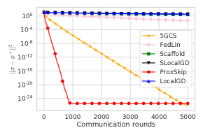
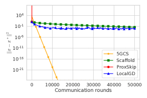
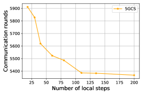
Figure 2: Performance of our 5GCS method without (left) and with (middle) CS. The plot on the right shows that 5GCS achieves optimal communication complexity with a (relatively) small number of local GD steps, as predicted by Theorem 3.3.

3.8 Relation between the # of communication rounds $T$ on the # of local steps $K$

We now study the dependence of the # of communication rounds $T$ on the # of local steps $K$ used by GD as the LT subroutine. We first show in Theorem 3.8 that with merely $K=\mathcal{O}\left(\log\frac{L}{\mu}\right)$ local GD steps we can improve the communication complexity from $T=\tilde{O}\left(\frac{{M}}{{C}}\frac{L}{\mu}\right)$ (provided in Theorem 3.5) to $T=\tilde{O}\left(\frac{{M}}{{C}}+\frac{L}{\mu}\right)$.

Theorem 3.8.

Consider Algorithm 1 (5GCS) with the LT solver being GD. Let ${\gamma}=\frac{3}{16L}$ and ${\tau}=\frac{8L}{3{M}}.$ With these stepsizes, if LT is performed via

$$\textstyle K\geq\left(2+\frac{3{M}L_{F}}{4L}\right)\log\left(4\frac{L}{\mu}\right)=\mathcal{O}\left(\log\frac{L}{\mu}\right)$$

steps of GD, then

$$\textstyle T \textstyle\geq\max\left\{1+\frac{16}{3}\frac{L}{\mu},\frac{{M}}{{C}}+\frac{3{M}}{8{C}}\frac{{M}L_{F}}{L}\right\}\log\frac{1}{\epsilon}$$

$$\textstyle=\tilde{\mathcal{O}}\left(\frac{{M}}{{C}}+\frac{L}{\mu}\right)$$

communication rounds suffice to find an $\varepsilon$-solution.

In Theorem 3.3 we showed that an accelerated communication complexity can be achieved with merely $K={\mathcal{O}}\left(\sqrt{\frac{{C}}{{M}}\frac{L}{\mu}}\log\frac{L}{\mu}\right)$ local GD steps. However, the behavior of $T$ on the interval between $K=\mathcal{O}\left(\log\frac{L}{\mu}\right)$ (studied in Theorem 3.8) and $K={\mathcal{O}}\left(\sqrt{\frac{{C}}{{M}}\frac{L}{\mu}}\log\frac{L}{\mu}\right)$ was not studied there. We shall do so now.

Theorem 3.9.

Consider Algorithm 1 (5GCS) with the LT solver being GD, which we run for

$$\textstyle K\geq K(\alpha)\coloneqq 2\alpha\log\left(\frac{4L}{\mu}\right)$$ (4)

iterations, where $\alpha$ is any constant satisfying

$$\textstyle 1<\alpha<1+\frac{3}{8}\sqrt{\frac{{C}}{{M}}\frac{L}{\mu}}.$$

Let ${\gamma}=\frac{1}{2{M}{\tau}}$ and ${\tau}=\max\left\{\frac{L}{{M}(\alpha-1)},\frac{8}{3}\sqrt{\frac{L\mu}{{M}{C}}}\right\}.$ Then for the Lyapunov function

$$\textstyle\Psi^{t}\coloneqq\frac{1}{{\gamma}}\left\|x^{t}-x^{\star}\right\|^{2}+\frac{{M}}{{C}}\left(\frac{1}{{\tau}}+\frac{1}{L_{F}}\right)\left\|u^{t}-u^{\star}\right\|^{2},$$

the iterates of the method satisfy $\mathbb{E}\!\left[\Psi^{T}\right]\leq(1-\rho)^{T}\Psi^{0},$ where $\rho\coloneqq\min\left\{\frac{{\gamma}\mu}{1+{\gamma}\mu},\frac{{C}}{{M}}\frac{{\tau}}{(L_{F}+{\tau})}\right\}<1.$

Corollary 3.10.

Choose any $0<\varepsilon<1$. In order to guarantee $\mathbb{E}\!\left[\Psi^{T}\right]\leq\varepsilon\Psi^{0}$, it suffices to take

$$\textstyle T\geq\max\left\{1+\frac{2L}{\left(\alpha-1\right)\mu},\frac{{M}}{{C}}\alpha\right\}\log\frac{1}{\epsilon}.$$

Note that if $\alpha\leq\frac{{M}+{C}}{2{M}}+\sqrt{\frac{2L{C}}{\mu{M}}+\left(\frac{{M}-{C}}{2{M}}\right)^{2}}$, then

$$\textstyle T\geq T(\alpha)\coloneqq\left(1+\frac{2}{\alpha-1}\frac{L}{\mu}\right)\log\frac{1}{\varepsilon}.$$

Theorem 3.9 and Corollary 3.10 imply that as long as $K\geq K(\alpha)$ and $T\geq T(\alpha)$, then ${\mathbb{E}}[\Psi^{T}]\leq\varepsilon\Psi^{0}$. By substituting $\alpha=\frac{K(\alpha)}{2\log\frac{4L}{\mu}}$ (see $\left(\ref{eq:h9y98fd8hfd}\right)$) to the expression for $T(\alpha)$, we get

$$\textstyle T(\alpha)=\left(1+\frac{4\log\frac{4L}{\mu}}{K(\alpha)-2\log\frac{4L}{\mu}}\frac{L}{\mu}\right)\log\frac{1}{\varepsilon}={\mathcal{O}}(\frac{1}{K(\alpha)})\log\frac{1}{\varepsilon}.$$

This inverse dependence of $T(\alpha)$ on $K(\alpha)$ can be observed empirically; see Figure 2 (right).

4 Experiments

We consider $\ell_{2}$-regularized logistic regression,

$$\textstyle f(x)=\frac{1}{{M}N}\sum\limits_{m=1}^{{M}}\sum\limits_{i=1}^{N}\log\left(1+e^{\left(-b_{m,i}a_{m,i}^{\top}x\right)}\right)+\frac{\lambda}{2}\|x\|^{2},$$

where $a_{m,i}\in\mathbb{R}^{d}$ and $b_{m,i}\in\{-1,+1\}$ are the data samples and labels, ${M}$ is the number of clients and $N$ is the number of data points per client. Following Malinovsky et al. (2022), we set $\lambda=10^{-3}L$, where $L$ is as in Assumption 1. We chose to highlight a representative experiment on the a1a dataset from the LibSVM library (Chang and Lin, 2011). All algorithms were implemented in Python utilizing the RAY package to simulate parallelization.

4.1 Full participation (${C}={M}$)

As a sanity check, we first perform an experiment in the full participation regime ${C}={M}=5$, comparing our method 5GCS with LocalGD (3^rd generation), Scaffold, SLocalGD and FedLin (4^th generation) and ProxSkip (5^th generation). We used theoretical stepsizes. For ProxSkip we used the optimal communication probability parameter $p=\nicefrac{{1}}{{\sqrt{\kappa}}}$, where $\kappa=\nicefrac{{L}}{{\mu}}$. In the case of all 4^th generation LT methods and LocalGD, the theoretical rate does not depend on number of local steps $K$. In our experiments we used the same number of local steps $K=\nicefrac{{1}}{{p}}=\sqrt{\kappa}$ for all competing methods. Figure 2 (left) clearly shows that 5GCS has accelerated communication complexity, outperforming all 4^th and 3^rd generation LT methods by a large margin. However, due to a small numerical constant for the stepsize in our theory $\left(\nicefrac{{3}}{{16}}\right)$, 5GCS converges more slowly than ProxSkip, which shows excellent performance.

4.2 Client sampling (${C}<{M}$)

Our key contribution is to bring client sampling (CS) to the world of 5^th generation LT methods. Once CS is required, ProxSkip and APDA-Inexact fall out of the competition as they do not support CS. We therefore compare our method 5GCS with 4^th and 3^rd generation LT methods supporting CS: we have chosen Scaffold and LocalGD. We set ${M}=15$ and ${C}=3$ and used theoretical parameters. Figure 2 (middle) shows that ProxSkip diverges in the CS regime, as expected. Moreover, 5GCS significantly outperforms the competing methods.

4.3 Dependence of $T$ on $K$

In this experiment we set $\lambda=5\cdot 10^{-4}L$ and run our method 5GCS (with GD as the LT solver) with $K$ ranging from $2\log\left(4\frac{L}{\mu}\right)$ to $\left(\frac{3}{4}\sqrt{\frac{{C}}{{M}}\frac{L}{\mu}}\right)\log\left(4\frac{L}{\mu}\right)$; plus an extra choice of $K=200$ steps. Figure 2 (right) shows that after $K\approx 110$ local GD steps, the comm. complexity virtually stops improving. This corresponds with our theory which shows that to obtain the optimal complexity, it suffices to take $K=\mathcal{O}\left(\left(\frac{3}{4}\sqrt{\frac{{C}}{{M}}\frac{L}{\mu}}\right)\log\left(4\frac{L}{\mu}\right)\right)$ local GD steps (see Theorem 3.3).

Appendix

Appendix A Basic Inequalities

A.1 Young’s inequalities

For all $x,y\in\mathbb{R}^{d}$ and all $a>0$, we have

$$\langle x,y\rangle\leq\frac{a\left\|x\right\|^{2}}{2}+\frac{\left\|y\right\|^{2}}{2a},$$ (5)

$$\left\|x+y\right\|^{2}\leq 2\left\|x\right\|^{2}+2\left\|y\right\|^{2},$$ (6)

$$\frac{1}{2}\left\|x\right\|^{2}-\left\|y\right\|^{2}\leq\left\|x+y\right\|^{2}.$$ (7)

A.2 Variance decomposition

For a random vector $\mathrm{X}\in\mathbb{R}^{d}$ (with finite second moment) and any $c\in\mathbb{R}^{d}$, the variance of $X$ can be decomposed as

$$\mathbb{E}\!\left[\left\|\mathrm{X}-\mathbb{E}\!\left[\mathrm{X}\right]\right\|^{2}\right]=\mathbb{E}\!\left[\left\|\mathrm{X}-c\right\|^{2}\right]-\left\|\mathbb{E}\!\left[\mathrm{X}\right]-c\right\|^{2}.$$ (8)

A.3 Compressor variance

An unbiased randomized mapping ${\mathcal{C}}:\mathbb{R}^{d}\to\mathbb{R}^{d}$ has conic variance if there exists $\omega\geq 0$ such that

$$\mathbb{E}\!\left[\left\|\mathcal{C}(x)-x\right\|^{2}\right]\leq\omega\left\|x\right\|^{2}$$ (9)

for all $x\in\mathbb{R}^{d}.$

A.4 Convexity and $L$-smoothness

Suppose $\phi\colon\mathbb{R}^{d}\to\mathbb{R}$ is $L$-smooth and convex. Then

$$\frac{1}{L}\left\|\nabla\phi(x)-\nabla\phi(y)\right\|^{2}\leq\langle\nabla\phi(x)-\nabla\phi(y),x-y\rangle$$ (10)

for all $x,y\in\mathbb{R}^{d}$.

A.5 Client Sampling Operator

Definition 1 (Client Sampling Operator).

The client sampling operator is the randomized mapping $\mathcal{P}:\mathbb{R}^{{M}d}\to\mathbb{R}^{{M}d}$ defined as follows. We choose a random subset $S\subseteq\left\{1,\dots,{M}\right\}$ of size ${C}\in\{1,\dots,{M}\}$ uniformly at random, and for $v=\left(v_{1},\dots,v_{M}\right)\in\mathbb{R}^{{M}d}$, where $v_{m}\in\mathbb{R}^{d}$ for all $m$, we define

$$\mathcal{P}(v)\coloneqq\left(\mathcal{P}_{1}(v_{1}),\dots,\mathcal{P}_{M}(v_{M})\right),$$

where

$$\mathcal{P}_{m}(v_{m})\coloneqq\begin{cases}\frac{{M}}{{C}}v_{m}\in\mathbb{R}^{d}&\quad\text{for}\quad m\in S,\\ 0\in\mathbb{R}^{d}&\quad\text{otherwise.}\end{cases}$$

The client sampling operatoradmits the following identity:

$$\mathbb{E}\!\left[\left\|{{H}}^{\top}\left(\mathcal{P}(v)-v\right)\right\|^{2}\right]=\frac{{M}}{{C}}\frac{{M}-{C}}{{M}-1}\sum_{m=1}^{{M}}\left\|v_{m}\right\|^{2}-\frac{{M}-{C}}{{C}\left({M}-1\right)}\left\|\sum_{m=1}^{{M}}v_{m}\right\|^{2},$$ (11)

where ${{H}}$ was defined in Section 3.2, and $v=\left(v_{1},\dots,v_{M}\right)\in\mathbb{R}^{{M}d}$ and $v_{m}\in\mathbb{R}^{d}$.

Proof.

Let $\mathbb{E}_{S}$ denote expectation with respect to the random set $S$. We can write

$$\mathbb{E}\!\left[\left\|{{H}}^{\top}\left(\mathcal{P}(v)-v\right)\right\|^{2}\right] = \mathbb{E}\!\left[\left\|\sum_{m=1}^{{M}}\left(\mathcal{P}_{m}(v_{m})-v_{m}\right)\right\|^{2}\right]=\mathbb{E}_{S}\!\left[\left\|\sum_{m\in S}\frac{{M}}{{C}}v_{m}-\sum_{m=1}^{{M}}v_{m}\right\|^{2}\right]$$

$$= \frac{{M}^{2}}{{C}^{2}}\mathbb{E}_{S}\!\left[\left\|\sum_{m\in S}v_{m}\right\|^{2}\right]+\left\|\sum_{m=1}^{{M}}v_{m}\right\|^{2}-\frac{2{M}}{{C}}\mathbb{E}_{S}\!\left[\left\langle\sum_{m\in S}v_{m},\sum_{m=1}^{{M}}v_{m}\right\rangle\right]$$

$$= \frac{{M}^{2}}{{C}^{2}}\mathbb{E}_{S}\!\left[\sum_{m\in S}\left\|v_{m}\right\|^{2}\right]+\frac{{M}^{2}}{{C}^{2}}\mathbb{E}_{S}\!\left[\sum_{m\in S}\sum_{m^{\prime}\in S,\neq m}\left\langle v_{m},v_{m^{\prime}}\right\rangle\right]-\left\|\sum_{m=1}^{{M}}v_{m}\right\|^{2}.$$

By computing the expectation on the right hand side, we get

$$\mathbb{E}\!\left[\left\|\sum_{m=1}^{{M}}\left(\mathcal{P}_{m}(v_{m})-v_{m}\right)\right\|^{2}\right] = \frac{{M}}{{C}}\left\|\sum_{m=1}^{{M}}v_{m}\right\|^{2}+\frac{{M}}{{C}}\frac{{C}-1}{{M}-1}\sum_{m=1}^{{M}}\sum_{m^{\prime}=1,\neq m}^{{M}}\left\langle v_{m},v_{m^{\prime}}\right\rangle-\left\|\sum_{m=1}^{{M}}v_{m}\right\|^{2}$$

$$= \frac{{M}}{{C}}\left(1-\frac{{C}-1}{{M}-1}\right)\left\|\sum_{m=1}^{{M}}v_{m}\right\|^{2}+\left(\frac{{M}\left({C}-1\right)}{{C}\left({M}-1\right)}-1\right)\left\|\sum_{m=1}^{{M}}v_{m}\right\|^{2}$$

$$= \frac{{M}}{{C}}\left(\frac{{M}-{C}}{{M}-1}\right)\left\|\sum_{m=1}^{{M}}v_{m}\right\|^{2}-\frac{{M}-{C}}{{C}\left({M}-1\right)}\left\|\sum_{m=1}^{{M}}v_{m}\right\|^{2}.$$

∎

A.6 Dual Problem and Saddle-Point Reformulation

Then the saddle function reformulation of $\left(\ref{eq:main-new}\right)$ is:

$$\mathrm{Find}\ (x^{\star},(u_{m}^{\star})_{m=1}^{M})\in\arg\min_{x\in\mathbb{R}^{d}}\max_{u\in\mathbb{R}^{{M}d}}\,\left(\frac{\mu}{2}\left\|x\right\|^{2}+\sum_{m=1}^{M}\left\langle x,u_{m}\right\rangle-\sum_{m=1}^{M}F_{m}^{*}(u_{m})\right).$$ (12)

To ensure well-posedness of these problems, we need to assume that there exists $x^{\star}\in\mathbb{R}^{d}$ s.t.:

$$0=\mu x^{\star}+\sum_{m=1}^{{M}}\nabla F_{m}(x^{\star}).$$ (13)

Which is equivalent to $\left(\ref{eq:main}\right)$, having a solution, which it does (unique in fact) as each $f_{m}$ is $\mu$-strongly convex. By first order optimality condition $x^{\star}$ and $u^{\star}$ that are solution to $\left(\ref{saddlenew}\right)$, satisfy:

$$\left\{\begin{array}[]{l}0=\mu x^{\star}+\sum_{m=1}^{M}u_{m}^{\star}\\ {{H}}x^{\star}\in\partial F^{*}(u^{\star})\end{array}\right..$$ (14)

Where the latter in $\left(\ref{fooc}\right)$ is equivalent to:

$$\nabla F({{H}}x^{\star})=u^{\star}.$$ (15)

Throughout, this section we will denote by $\mathcal{F}_{t}$ for all $t\geq 0$ the $\sigma$-algebra generated by the collection of $\left(\mathbb{R}^{d}\times\mathbb{R}^{d{M}}\right)$-valued random variables $\left(x^{0},u^{0}\right),\dots,\left(x^{t},u^{t}\right).$

Appendix B Analysis of 5GCS_∞

Algorithm 2 5GCS with $\infty$ local GD steps (a.k.a. Minibatch Point-SAGA)

1:  input: initial points $x^{0}\in\mathbb{R}^{d}$, $u_{m}^{0}\in\mathbb{R}^{d}$ for all $m=\{1,\dots,{M}\}$;

2:  stepsize ${\gamma}>0$, ${\tau}>0$; ${C}\in\{1,\dots,{M}\}$

3:  $v^{0}\coloneqq\sum_{m=1}^{M}u_{m}^{0}$

4:  for $t=0,1,\ldots$ do

5:     $\hat{x}^{t}\coloneqq\frac{1}{1+{\gamma}\mu}\left(x^{t}-{\gamma}v^{t}\right)$

6:     Pick $S^{t}\subset\{1,\ldots,{M}\}$ of size ${C}$ uniformly at random

7:     for $m\in S^{t}$ do

8:        $u_{m}^{t+1}\coloneqq u_{m}^{t}+{\tau}\hat{x}^{t}-{\tau}\mathrm{prox}_{\frac{1}{{\tau}}F_{m}}\left(\hat{x}^{t}+\frac{1}{{\tau}}u_{m}^{t}\right)$

9:     end for

10:     for $m\in\{1,\ldots,{M}\}\backslash S^{t}$ do

11:        $u_{m}^{t+1}\coloneqq u_{m}^{t}$

12:     end for

13:     $v^{t+1}\coloneqq\sum_{m=1}^{M}u_{m}^{t+1}$

14:     $x^{t+1}\coloneqq\hat{x}^{t}-{\gamma}\frac{{M}}{{C}}(v^{t+1}-v^{t})$

15:  end for

Theorem B.1.

Consider Algorithm 1 (5GCS) with the LT solver being GD run for $K=+\infty$ iterations (this is equivalent to Algorithm 2; we shall also call the method 5GCS_∞). Let ${\gamma}>0$, ${\tau}>0$ and ${\gamma}{\tau}\leq\frac{1}{{M}}$. Then for the Lyapunov function

$$\Psi^{t}\coloneqq\frac{1}{{\gamma}}\left\|x^{t}-x^{\star}\right\|^{2}+\frac{{M}}{{C}}\left(\frac{1}{{\tau}}+2\frac{1}{L_{F}}\right)\left\|u^{t}-u^{\star}\right\|^{2},$$

the iterates of the method satisfy $\mathbb{E}\!\left[\Psi^{T}\right]\leq(1-\rho)^{T}\Psi^{0},$ where $\rho\coloneqq\min\left(\frac{{\gamma}\mu}{1+{\gamma}\mu},\frac{{C}}{{M}}\frac{2{\tau}}{L_{F}+2{\tau}}\right)<1.$

Proof.

Noting that updates for $u^{t+1}$ and $x^{t+1}$ can be written as

$$u^{t+1}\coloneqq u^{t}+\tfrac{1}{1+\omega}\mathcal{P}^{t}\left(\hat{u}^{t+1}-u^{t}\right),$$ (16)

$$x^{t+1}=\hat{x}^{t}-{\gamma}\frac{{M}}{{C}}{{H}}^{\top}\left(u^{t+1}-u^{t}\right)$$ (17)

where $\mathcal{P}^{t}$ is the client sampling operator, $\omega=\frac{{M}}{{C}}-1$ and $\hat{u}^{t+1}=\mathrm{prox}_{{\tau}F^{*}}\left(u^{t}+{\tau}{{H}}\hat{x}^{t}\right)$. We can use variance decomposition and Proposition 1 from Condat and Richtárik (2021) to write

$$\mathbb{E}\!\left[\left\|x^{t+1}-x^{\star}\right\|^{2}\;|\;\mathcal{F}_{t}\right] \overset{(\ref{vardec})}{=} \left\|\mathbb{E}\!\left[x^{t+1}\;|\;\mathcal{F}_{t}\right]-x^{\star}\right\|^{2}+\mathbb{E}\!\left[\left\|x^{t+1}-\mathbb{E}\!\left[x^{t+1}\;|\;\mathcal{F}_{t}\right]\right\|^{2}\;|\;\mathcal{F}_{t}\right]$$ (18)

$$\overset{(\ref{xupdate})}{=} \left\|\mathbb{E}\!\left[\hat{x}^{t}-{\gamma}\frac{{M}}{{C}}(v^{t+1}-v^{t})\;|\;\mathcal{F}_{t}\right]-x^{\star}\right\|^{2}+\mathbb{E}\!\left[\left\|x^{t+1}-\mathbb{E}\!\left[x^{t+1}\;|\;\mathcal{F}_{t}\right]\right\|^{2}\;|\;\mathcal{F}_{t}\right]$$

$$= \left\|\hat{x}^{t}-x^{\star}-{\gamma}\frac{{M}}{{C}}\mathbb{E}\!\left[{{H}}^{\top}\left(u^{t+1}-u^{t}\right)\;|\;\mathcal{F}_{t}\right]\right\|^{2}+\mathbb{E}\!\left[\left\|x^{t+1}-\mathbb{E}\!\left[x^{t+1}\;|\;\mathcal{F}_{t}\right]\right\|^{2}\;|\;\mathcal{F}_{t}\right]$$

$$= \left\|\hat{x}^{t}-x^{\star}-{\gamma}{{H}}^{\top}\left(\hat{u}^{t+1}-u^{t}\right)\right\|^{2}+\mathbb{E}\!\left[\left\|x^{t+1}-\mathbb{E}\!\left[x^{t+1}\;|\;\mathcal{F}_{t}\right]\right\|^{2}\;|\;\mathcal{F}_{t}\right]$$

$$\overset{(\ref{PP})}{=} \underbrace{\left\|\hat{x}^{t}-x^{\star}-{\gamma}{{H}}^{\top}\left(\hat{u}^{t+1}-u^{t}\right)\right\|^{2}}_{X}+{\gamma}^{2}\omega_{\mathrm{ran}}\left\|\hat{u}^{t+1}-u^{t}\right\|^{2}$$

$$-{\gamma}^{2}\zeta\left\|{{H}}^{\top}\left(\hat{u}^{t+1}-u^{t}\right)\right\|^{2}.$$

where

$$\omega_{\mathrm{ran}}=\frac{{M}({M}-{C})}{{C}({M}-1)},\quad\zeta=\frac{{M}-{C}}{{C}({M}-1)}.$$

Moreover, using $\left(\ref{fooc}\right)$ and the definition of $\hat{x}^{t}$, we have

$$(1+{\gamma}\mu)\hat{x}^{t}=x^{t}-{\gamma}{{H}}^{\top}u^{t},$$ (19)

$$(1+{\gamma}\mu)x^{\star}=x^{\star}-{\gamma}{{H}}^{\top}u^{\star}.$$ (20)

Using $\left(\ref{opt13}\right)$ and $\left(\ref{opt23}\right)$ we obtain

$$X = \left\|\hat{x}^{t}-x^{\star}\right\|^{2}+{\gamma}^{2}\left\|{{H}}^{\top}\left(\hat{u}^{t+1}-u^{t}\right)\right\|^{2}-2{\gamma}\left\langle\hat{x}^{t}-x^{\star},{{H}}^{\top}\left(\hat{u}^{t+1}-u^{t}\right)\right\rangle$$ (21)

$$\leq (1+{\gamma}\mu)\left\|\hat{x}^{t}-x^{\star}\right\|^{2}+{\gamma}^{2}\left\|{{H}}^{\top}\left(\hat{u}^{t+1}-u^{t}\right)\right\|^{2}$$

$$-2{\gamma}\left\langle\hat{x}^{t}-x^{\star},{{H}}^{\top}\left(\hat{u}^{t+1}-u^{\star}\right)\right\rangle+2{\gamma}\left\langle\hat{x}^{t}-x^{\star},{{H}}^{\top}\left(u^{t}-u^{\star}\right)\right\rangle$$

$$\overset{(\ref{opt13})+(\ref{opt23})}{=} \left\langle x^{t}-x^{\star}-{\gamma}{{H}}^{\top}\left(u^{t}-u^{\star}\right),\hat{x}^{t}-x^{\star}\right\rangle+{\gamma}^{2}\left\|{{H}}^{\top}\left(\hat{u}^{t+1}-u^{t}\right)\right\|^{2}$$

$$-2{\gamma}\left\langle\hat{x}^{t}-x^{\star},{{H}}^{\top}\left(\hat{u}^{t+1}-u^{\star}\right)\right\rangle+\left\langle\hat{x}^{t}-x^{\star},2{\gamma}{{H}}^{\top}\left(u^{t}-u^{\star}\right)\right\rangle$$

$$= \left\langle x^{t}-x^{\star}+{\gamma}{{H}}^{\top}\left(u^{t}-u^{\star}\right),\hat{x}^{t}-x^{\star}\right\rangle+{\gamma}^{2}\left\|{{H}}^{\top}\left(\hat{u}^{t+1}-u^{t}\right)\right\|^{2}$$

$$-2{\gamma}\left\langle\hat{x}^{t}-x^{\star},{{H}}^{\top}\left(\hat{u}^{t+1}-u^{\star}\right)\right\rangle$$

$$\overset{(\ref{opt13})+(\ref{opt23})}{=} \frac{1}{1+{\gamma}\mu}\left\langle x^{t}-x^{\star}+{\gamma}{{H}}^{\top}\left(u^{t}-u^{\star}\right),x^{t}-x^{\star}-{\gamma}{{H}}^{\top}\left(u^{t}-u^{\star}\right)\right\rangle$$

$$+{\gamma}^{2}\left\|{{H}}^{\top}\left(\hat{u}^{t+1}-u^{t}\right)\right\|^{2}-2{\gamma}\left\langle\hat{x}^{t}-x^{\star},{{H}}^{\top}\left(\hat{u}^{t+1}-u^{\star}\right)\right\rangle$$

$$= \frac{1}{1+{\gamma}\mu}\left\|x^{t}-x^{\star}\right\|^{2}-\frac{{\gamma}^{2}}{1+{\gamma}\mu}\left\|{{H}}^{\top}\left(u^{t}-u^{\star}\right)\right\|^{2}$$

$$+{\gamma}^{2}\left\|{{H}}^{\top}\left(\hat{u}^{t+1}-u^{t}\right)\right\|^{2}-2{\gamma}\left\langle\hat{x}^{t}-x^{\star},{{H}}^{\top}\left(\hat{u}^{t+1}-u^{\star}\right)\right\rangle.$$

Combining $\left(\ref{xbound31}\right)$ and $\left(\ref{long31}\right)$

$$\mathbb{E}\!\left[\left\|x^{t+1}-x^{\star}\right\|^{2}\;|\;\mathcal{F}_{t}\right] \leq \frac{1}{1+{\gamma}\mu}\left\|x^{t}-x^{\star}\right\|^{2}-\frac{{\gamma}^{2}}{1+{\gamma}\mu}\left\|{{H}}^{\top}\left(u^{t}-u^{\star}\right)\right\|^{2}$$ (22)

$$+{\gamma}^{2}(1-\zeta)\left\|{{H}}^{\top}\left(\hat{u}^{t+1}-u^{t}\right)\right\|^{2}-2{\gamma}\left\langle\hat{x}^{t}-x^{\star},{{H}}^{\top}\left(\hat{u}^{t+1}-u^{\star}\right)\right\rangle$$

$$+{\gamma}^{2}\omega_{\mathrm{ran}}\left\|\hat{u}^{t+1}-u^{t}\right\|^{2}.$$

On the other hand using the variance decomposition and conic variance of $\mathcal{P}^{t}$

$$\mathbb{E}\!\left[\left\|u^{t+1}-u^{\star}\right\|^{2}\;|\;\mathcal{F}_{t}\right] \overset{(\ref{vardec})+(\ref{cvar})}{\leq} \left\|u^{t}-u^{\star}+\frac{1}{1+\omega}\left(\hat{u}^{t+1}-u^{t}\right)\right\|^{2}+\frac{\omega}{(1+\omega)^{2}}\left\|\hat{u}^{t+1}-u^{t}\right\|^{2}$$ (23)

$$= \left\|\frac{\omega}{1+\omega}(u^{t}-u^{\star})+\frac{1}{1+\omega}\left(\hat{u}^{t+1}-u^{\star}\right)\right\|^{2}+\frac{\omega}{(1+\omega)^{2}}\left\|\hat{u}^{t+1}-u^{\star}-(u^{t}-u^{\star})\right\|^{2}$$

$$= \frac{\omega^{2}}{(1+\omega)^{2}}\left\|u^{t}-u^{\star}\right\|^{2}+\frac{1}{(1+\omega)^{2}}\left\|\hat{u}^{t+1}-u^{\star}\right\|^{2}$$

$$+\frac{2\omega}{(1+\omega)^{2}}\left\langle u^{t}-u^{\star},\hat{u}^{t+1}-u^{\star}\right\rangle+\frac{\omega}{(1+\omega)^{2}}\left\|\hat{u}^{t+1}-u^{\star}\right\|^{2}$$

$$+\frac{\omega}{(1+\omega)^{2}}\left\|u^{t}-u^{\star}\right\|^{2}-\frac{2\omega}{(1+\omega)^{2}}\left\langle u^{t}-u^{\star},\hat{u}^{t+1}-u^{\star}\right\rangle$$

$$= \frac{1}{1+\omega}\left\|\hat{u}^{t+1}-u^{\star}\right\|^{2}+\frac{\omega}{1+\omega}\left\|u^{t}-u^{\star}\right\|^{2}.$$

Let $(s_{m}^{t+1})_{m=1}^{M}\in\partial F^{*}(\hat{u}^{t+1})$ be such that $\hat{u}_{m}^{t+1}=u_{m}^{t}+{\tau}\hat{x}^{t}-{\tau}s_{m}^{t+1}$; $s^{t+1}$ exists and is unique. We also define $s_{m}^{\star}\coloneqq x^{\star}$; we have $s^{\star}\in\partial F^{*}(u^{\star})$. Therefore,

$$\left\|\hat{u}^{t+1}-u^{\star}\right\|^{2} = \left\|(u^{t}-u^{\star})+(\hat{u}^{t+1}-u^{t})\right\|^{2}$$ (24)

$$= \left\|u^{t}-u^{\star}\right\|^{2}+\left\|\hat{u}^{t+1}-u^{t}\right\|^{2}+2\left\langle u^{t}-u^{\star},\hat{u}^{t+1}-u^{t}\right\rangle$$

$$= \left\|u^{t}-u^{\star}\right\|^{2}+2\left\langle\hat{u}^{t+1}-u^{\star},\hat{u}^{t+1}-u^{t}\right\rangle-\left\|\hat{u}^{t+1}-u^{t}\right\|^{2}$$

$$= \left\|u^{t}-u^{\star}\right\|^{2}-\left\|\hat{u}^{t+1}-u^{t}\right\|^{2}+2{\tau}\left\langle{{H}}^{\top}\left(\hat{u}^{t+1}-u^{\star}\right),\hat{x}^{t}-x^{\star}\right\rangle$$

$$-2{\tau}\left\langle\hat{u}^{t+1}-u^{\star},s^{t+1}-s^{\star}\right\rangle.$$

Combining $\left(\ref{ubound}\right)$, $\left(\ref{ubound31}\right)$ and $\left(\ref{xbnd31}\right)$ gives

$$\frac{1}{{\gamma}}\mathbb{E}\!\left[\left\|x^{t+1}-x^{\star}\right\|^{2}\;|\;\mathcal{F}_{t}\right] + \frac{1+\omega}{{\tau}}\mathbb{E}\!\left[\left\|u^{t+1}-u^{\star}\right\|^{2}\;|\;\mathcal{F}_{t}\right]$$

$$\leq \frac{1}{{\gamma}(1+{\gamma}\mu)}\left\|x^{t}-x^{\star}\right\|^{2}-\frac{{\gamma}}{1+{\gamma}\mu}\left\|{{H}}^{\top}\left(u^{t}-u^{\star}\right)\right\|^{2}$$

$$+{\gamma}(1-\zeta)\left\|{{H}}^{\top}\left(\hat{u}^{t+1}-u^{t}\right)\right\|^{2}-2\left\langle\hat{x}^{t}-x^{\star},{{H}}^{\top}\left(\hat{u}^{t+1}-u^{\star}\right)\right\rangle$$

$$+{\gamma}\omega_{\mathrm{ran}}\left\|\hat{u}^{t+1}-u^{t}\right\|^{2}+\frac{1}{{\tau}}\left\|u^{t}-u^{\star}\right\|^{2}-\frac{1}{{\tau}}\left\|\hat{u}^{t+1}-u^{t}\right\|^{2}$$

$$+2\left\langle{{H}}^{\top}\left(\hat{u}^{t+1}-u^{\star}\right),\hat{x}^{t}-x^{\star}\right\rangle-2\left\langle\hat{u}^{t+1}-u^{\star},s^{t+1}-s^{\star}\right\rangle$$

$$+\frac{\omega}{{\tau}}\left\|u^{t}-u^{\star}\right\|^{2}$$

$$\leq \frac{1}{{\gamma}(1+{\gamma}\mu)}\left\|x^{t}-x^{\star}\right\|^{2}-\frac{{\gamma}}{1+{\gamma}\mu}\left\|{{H}}^{\top}\left(u^{t}-u^{\star}\right)\right\|^{2}$$

$$+\frac{1+\omega}{{\tau}}\left\|u^{t}-u^{\star}\right\|^{2}+\left({\gamma}\left((1-\zeta){M}+\omega_{\mathrm{ran}}\right)-\frac{1}{{\tau}}\right)\left\|\hat{u}^{t+1}-u^{t}\right\|^{2}$$

$$-2\left\langle\hat{u}^{t+1}-u^{\star},s^{t+1}-s^{\star}\right\rangle$$

$$\leq \frac{1}{{\gamma}(1+{\gamma}\mu)}\left\|x^{t}-x^{\star}\right\|^{2}-\frac{{\gamma}}{1+{\gamma}\mu}\left\|{{H}}^{\top}\left(u^{t}-u^{\star}\right)\right\|^{2}$$

$$+\frac{1+\omega}{{\tau}}\left\|u^{t}-u^{\star}\right\|^{2}-2\left\langle\hat{u}^{t+1}-u^{\star},s^{t+1}-s^{\star}\right\rangle.$$

By $\frac{1}{L_{F}}$-strong monotonicity of $\partial F^{*}$, $\left\langle\hat{u}^{t+1}-u^{\star},s^{t+1}-s^{\star}\right\rangle\geq\frac{1}{L_{F}}\left\|\hat{u}^{t+1}-u^{\star}\right\|^{2}$, and using $\left(\ref{ubound}\right)$,

$$\left\langle\hat{u}^{t+1}-u^{\star},s^{t+1}-s^{\star}\right\rangle\geq\frac{1}{L_{F}}\left((1+\omega)\mathbb{E}\!\left[\left\|u^{t+1}-u^{\star}\right\|^{2}\;|\;\mathcal{F}_{t}\right]-\omega\left\|u^{t}-u^{\star}\right\|^{2}\right).$$

Hence,

$$\frac{1}{{\gamma}}\mathbb{E}\!\left[\left\|x^{t+1}-x^{\star}\right\|^{2}\;|\;\mathcal{F}_{t}\right] + (1+\omega)\left(\frac{1}{{\tau}}+2\frac{1}{L_{F}}\right)\mathbb{E}\!\left[\left\|u^{t+1}-u^{\star}\right\|^{2}\;|\;\mathcal{F}_{t}\right]$$ (25)

$$\leq \frac{1}{{\gamma}(1+{\gamma}\mu)}\left\|x^{t}-x^{\star}\right\|^{2}+\left(\frac{1+\omega}{{\tau}}+2\omega\frac{1}{L_{F}}\right)\left\|u^{t}-u^{\star}\right\|^{2}$$

$$-\frac{{\gamma}}{1+{\gamma}\mu}\left\|{{H}}^{\top}\left(u^{t}-u^{\star}\right)\right\|^{2}.$$

Ignoring the last term in $\left(\ref{kkkk}\right)$, we obtain

$$\mathbb{E}\!\left[\Psi^{t+1}\right]\leq\max\left(\frac{1}{1+{\gamma}\mu},1-\frac{2{\tau}}{(1+\omega)(L_{F}+2{\tau})}\right)\mathbb{E}\!\left[\Psi^{t}\right].$$ (26)

∎

B.1 Proof of Corollary 3.2

Corollary B.2.

Choose any $0<\varepsilon<1$. If we choose ${\gamma}=\sqrt{\frac{2{C}}{L_{F}\mu{M}^{2}}}$ and ${\tau}=\sqrt{\frac{L_{F}\mu}{2{C}}}$, then in order to guarantee $\mathbb{E}\!\left[\Psi^{T}\right]\leq\varepsilon\Psi^{0}$, it suffices to take

$$T\geq\left(\frac{{M}}{{C}}+\sqrt{\frac{{M}}{{C}}\frac{L-\mu}{2\mu}}\right)\log\frac{1}{\varepsilon}=\tilde{{\mathcal{O}}}\left(\frac{{M}}{{C}}+\sqrt{\frac{{M}}{{C}}\frac{L}{\mu}}\right)$$

communication rounds.

Proof.

Firstly, note that choosing ${\gamma}=\sqrt{\frac{2{C}}{L_{F}\mu{M}^{2}}}$ and ${\tau}=\sqrt{\frac{L_{F}\mu}{2{C}}}$ we satisfy ${\gamma}{\tau}=\frac{1}{{M}}$, than that we get the contraction constant from the proof to be equal to:

$$\max\left\{1-\frac{\sqrt{\frac{2{C}\mu}{L_{F}{M}^{2}}}}{1+\sqrt{\frac{2{C}\mu}{L_{F}{M}^{2}}}},1-\frac{\sqrt{\frac{2L_{h}\mu}{{C}}}}{\frac{{M}}{{C}}\left(L_{F}+\sqrt{\frac{2L_{F}\mu}{{C}}}\right)}\right\} = \max\left\{1-\frac{\sqrt{2{C}\mu}}{{M}\sqrt{L_{F}}+\sqrt{2{C}\mu}},1-\frac{\sqrt{2{C}\mu}}{{M}\sqrt{L_{F}}+\sqrt{\frac{2\mu{M}^{2}}{{C}}}}\right\}$$

$$= 1-\frac{\sqrt{2{C}\mu}}{{M}\sqrt{L_{F}}+\sqrt{\frac{2\mu{M}^{2}}{{C}}}}.$$

This gives a rate of

$$T=\mathcal{O}\left(\frac{{M}\sqrt{L_{F}}+\sqrt{\frac{2\mu{M}^{2}}{{C}}}}{\sqrt{2{C}\mu}}\log\frac{1}{\varepsilon}\right)=\mathcal{O}\left(\left(\frac{{M}}{{C}}+\sqrt{\frac{(L-\mu){M}}{2\mu{C}}}\right)\log\frac{1}{\varepsilon}\right).$$

∎

Appendix C Analysis of 5GCS

Theorem C.1.

Consider Algorithm 1 (5GCS) with the LT solver being GD run for

$$K\geq\left(\frac{3}{4}\sqrt{\frac{{C}}{{M}}\frac{L}{\mu}}+2\right)\log\left(4\frac{L}{\mu}\right)$$

iterations. Let $0<{\gamma}\leq\frac{3}{16}\sqrt{\frac{{C}}{L\mu{M}}}$ and ${\tau}=\frac{1}{2{\gamma}{M}}$. Then for the Lyapunov function

$$\Psi^{t}\coloneqq\frac{1}{{\gamma}}\left\|x^{t}-x^{\star}\right\|^{2}+\frac{{M}}{{C}}\left(\frac{1}{{\tau}}+\frac{1}{L_{F}}\right)\left\|u^{t}-u^{\star}\right\|^{2},$$

the iterates of the method satisfy

$$\mathbb{E}\!\left[\Psi^{T}\right]\leq(1-\rho)^{T}\Psi^{0},$$

where $\rho\coloneqq\max\left\{\frac{{\gamma}\mu}{1+{\gamma}\mu},\frac{{C}}{{M}}\frac{{\tau}}{(L_{F}+{\tau})}\right\}<1.$

Proof.

Noting that updates for $u^{t+1}$ and $x^{t+1}$ can be written as

$$u^{t+1}\coloneqq u^{t}+\frac{1}{1+\omega}\mathcal{P}^{t}\left(\bar{u}^{t+1}-u^{t}\right),$$ (27)

$$x^{t+1}=\hat{x}^{t}-{\gamma}\left(\omega+1\right){{H}}^{\top}\left(u^{t+1}-u^{t}\right)$$ (28)

where $\mathcal{P}^{t}$ is the client sampling operator, $\omega=\frac{{M}}{{C}}-1$ and $\bar{u}^{t+1}=\nabla F(y^{K,t})$. Then using variance decomposition and Proposition 1 from (Condat and Richtárik, 2021), we obtain

$$\mathbb{E}\!\left[\left\|x^{t+1}-x^{\star}\right\|^{2}\;|\;\mathcal{F}_{t}\right] \overset{(\ref{vardec})}{=} \left\|\mathbb{E}\!\left[x^{t+1}\;|\;\mathcal{F}_{t}\right]-x^{\star}\right\|^{2}+\mathbb{E}\!\left[\left\|x^{t+1}-\mathbb{E}\!\left[x^{t+1}\;|\;\mathcal{F}_{t}\right]\right\|^{2}\;|\;\mathcal{F}_{t}\right]$$ (29)

$$\overset{(\ref{xupdate35})+(\ref{PP})}{=} \underbrace{\left\|\hat{x}^{t}-x^{\star}-{\gamma}{{H}}^{\top}(\bar{u}^{t+1}-u^{t})\right\|^{2}}_{X}+{\gamma}^{2}\omega_{\mathrm{ran}}\left\|\bar{u}^{t+1}-u^{t}\right\|^{2}$$

$$-{\gamma}^{2}\zeta\left\|{{H}}^{\top}(\bar{u}^{t+1}-u^{t})\right\|^{2},$$

where

$$\omega_{\mathrm{ran}}=\frac{{M}({M}-{C})}{{C}({M}-1)},\quad\zeta=\frac{{M}-{C}}{{C}({M}-1)}.$$

Moreover, using $\left(\ref{fooc}\right)$ and the definition of $\hat{x}^{t}$, we have

$$(1+{\gamma}\mu)\hat{x}^{t}=x^{t}-{\gamma}{{H}}^{\top}u^{t},$$ (30)

$$(1+{\gamma}\mu)x^{\star}=x^{\star}-{\gamma}{{H}}^{\top}u^{\star}.$$ (31)

Using $\left(\ref{opt1}\right)$ and $\left(\ref{opt2}\right)$ we obtain

$$X = \left\|\hat{x}^{t}-x^{\star}-{\gamma}{{H}}^{\top}(\bar{u}^{t+1}-u^{t})\right\|^{2}$$

$$= \left\|\hat{x}^{t}-x^{\star}\right\|^{2}+{\gamma}^{2}\left\|{{H}}^{\top}(\bar{u}^{t+1}-u^{t})\right\|^{2}-2{\gamma}\left\langle\hat{x}^{t}-x^{\star},{{H}}^{\top}(\bar{u}^{t+1}-u^{t})\right\rangle$$

$$= (1+{\gamma}\mu)\left\|\hat{x}^{t}-x^{\star}\right\|^{2}+{\gamma}^{2}\left\|{{H}}^{\top}(\bar{u}^{t+1}-u^{t})\right\|^{2}$$

$$-2{\gamma}\left\langle\hat{x}^{t}-x^{\star},{{H}}^{\top}(\bar{u}^{t+1}-u^{\star})\right\rangle+2{\gamma}\left\langle\hat{x}^{t}-x^{\star},{{H}}^{\top}(u^{t}-u^{\star})\right\rangle-{\gamma}\mu\left\|\hat{x}^{t}-x^{\star}\right\|^{2}$$

$$\overset{(\ref{opt1})+(\ref{opt2})}{=} \left\langle x^{t}-x^{\star}-{\gamma}{{H}}^{\top}(u^{t}-u^{\star}),\hat{x}^{t}-x^{\star}\right\rangle+{\gamma}^{2}\left\|{{H}}^{\top}(\bar{u}^{t+1}-u^{t})\right\|^{2}$$

$$-2{\gamma}\left\langle\hat{x}^{t}-x^{\star},{{H}}^{\top}(\bar{u}^{t+1}-u^{\star})\right\rangle+\left\langle\hat{x}^{t}-x^{\star},2{\gamma}{{H}}^{\top}(u^{t}-u^{\star})\right\rangle-{\gamma}\mu\left\|\hat{x}^{t}-x^{\star}\right\|^{2}.$$

This leads to

$$X = \left\langle x^{t}-x^{\star}+{\gamma}{{H}}^{\top}(u^{t}-u^{\star}),\hat{x}^{t}-x^{\star}\right\rangle$$ (32)

$$+{\gamma}^{2}\left\|{{H}}^{\top}(\bar{u}^{t+1}-u^{t})\right\|^{2}-2{\gamma}\left\langle\hat{x}^{t}-x^{\star},{{H}}^{\top}(\bar{u}^{t+1}-u^{\star})\right\rangle-{\gamma}\mu\left\|\hat{x}^{t}-x^{\star}\right\|^{2}$$

$$\overset{(\ref{opt1})+(\ref{opt2})}{=} \frac{1}{1+{\gamma}\mu}\left\langle x^{t}-x^{\star}+{\gamma}{{H}}^{\top}(u^{t}-u^{\star}),x^{t}-x^{\star}-{\gamma}{{H}}^{\top}(u^{t}-u^{\star})\right\rangle$$

$$+{\gamma}^{2}\left\|{{H}}^{\top}(\bar{u}^{t+1}-u^{t})\right\|^{2}-2{\gamma}\left\langle\hat{x}^{t}-x^{\star},{{H}}^{\top}(\bar{u}^{t+1}-u^{\star})\right\rangle-{\gamma}\mu\left\|\hat{x}^{t}-x^{\star}\right\|^{2}$$

$$= \frac{1}{1+{\gamma}\mu}\left\|x^{t}-x^{\star}\right\|^{2}-\frac{{\gamma}^{2}}{1+{\gamma}\mu}\left\|{{H}}^{\top}(u^{t}-u^{\star})\right\|^{2}$$

$$+{\gamma}^{2}\left\|{{H}}^{\top}(\bar{u}^{t+1}-u^{t})\right\|^{2}-2{\gamma}\left\langle\hat{x}^{t}-x^{\star},{{H}}^{\top}(\bar{u}^{t+1}-u^{\star})\right\rangle-{\gamma}\mu\left\|\hat{x}^{t}-x^{\star}\right\|^{2}.$$

Combining $\left(\ref{eq:starting_eq3.5}\right)$ and $\left(\ref{eq:long3.5}\right)$, we get

$$\mathbb{E}\!\left[\left\|x^{t+1}-x^{\star}\right\|^{2}\;|\;\mathcal{F}_{t}\right] \leq \frac{1}{1+{\gamma}\mu}\left\|x^{t}-x^{\star}\right\|^{2}-\frac{{\gamma}^{2}}{1+{\gamma}\mu}\left\|{{H}}^{\top}(u^{t}-u^{\star})\right\|^{2}$$

$$+{\gamma}^{2}(1-\zeta)\left\|{{H}}^{\top}(\bar{u}^{t+1}-u^{t})\right\|^{2}-2{\gamma}\left\langle\hat{x}^{t}-x^{\star},{{H}}^{\top}(\bar{u}^{t+1}-u^{\star})\right\rangle$$

$$+{\gamma}^{2}\omega_{\mathrm{ran}}\left\|\bar{u}^{t+1}-u^{t}\right\|^{2}-\frac{{\gamma}\mu}{{M}}\left\|{{H}}\hat{x}^{t}-{{H}}x^{\star}\right\|^{2}.$$

Note that we can have the update rule for $u$ as:

$$u^{t+1}\coloneqq u^{t}+\frac{1}{1+\omega}\mathcal{P}^{t}\left(\bar{u}^{t+1}-u^{t}\right),$$

where $\mathcal{P}^{t}$ is client sampling operator with parameter $\omega=\frac{{M}}{{C}}-1$. Using conic variance formula $\left(\ref{cvar}\right)$ of $\mathcal{P}^{t}$, we obtain

$$\mathbb{E}\!\left[\left\|u^{t+1}-u^{\star}\right\|^{2}\;|\;\mathcal{F}_{t}\right] \overset{(\ref{vardec})+(\ref{cvar})}{\leq} \left\|u^{t}-u^{\star}+\frac{1}{1+\omega}\left(\bar{u}^{t+1}-u^{t}\right)\right\|^{2}+\frac{\omega}{(1+\omega)^{2}}\left\|\bar{u}^{t+1}-u^{t}\right\|^{2}$$ (33)

$$= \frac{\omega^{2}}{(1+\omega)^{2}}\left\|u^{t}-u^{\star}\right\|^{2}+\frac{1}{(1+\omega)^{2}}\left\|\bar{u}^{t+1}-u^{\star}\right\|^{2}$$

$$+\frac{2\omega}{(1+\omega)^{2}}\left\langle u^{t}-u^{\star},\bar{u}^{t+1}-u^{\star}\right\rangle+\frac{\omega}{(1+\omega)^{2}}\left\|\bar{u}^{t+1}-u^{\star}\right\|^{2}$$

$$+\frac{\omega}{(1+\omega)^{2}}\left\|u^{t}-u^{\star}\right\|^{2}-\frac{2\omega}{(1+\omega)^{2}}\left\langle u^{t}-u^{\star},\bar{u}^{t+1}-u^{\star}\right\rangle$$

$$= \frac{1}{1+\omega}\left\|\bar{u}^{t+1}-u^{\star}\right\|^{2}+\frac{\omega}{1+\omega}\left\|u^{t}-u^{\star}\right\|^{2}.$$

Let us consider the first term in $\left(\ref{expu}\right)$:

$$\left\|\bar{u}^{t+1}-u^{\star}\right\|^{2} = \left\|(u^{t}-u^{\star})+(\bar{u}^{t+1}-u^{t})\right\|^{2}$$

$$= \left\|u^{t}-u^{\star}\right\|^{2}+\left\|\bar{u}^{t+1}-u^{t}\right\|^{2}+2\left\langle u^{t}-u^{\star},\bar{u}^{t+1}-u^{t}\right\rangle$$

$$= \left\|u^{t}-u^{\star}\right\|^{2}+2\left\langle\bar{u}^{t+1}-u^{\star},\bar{u}^{t+1}-u^{t}\right\rangle-\left\|\bar{u}^{t+1}-u^{t}\right\|^{2}.$$

Combining the terms together, we get

$$\mathbb{E}\!\left[\left\|u^{t+1}-u^{\star}\right\|^{2}\;|\;\mathcal{F}_{t}\right]\leq\left\|u^{t}-u^{\star}\right\|^{2}+\frac{1}{1+\omega}\left(2\left\langle\bar{u}^{t+1}-u^{\star},\bar{u}^{t+1}-u^{t}\right\rangle-\left\|\bar{u}^{t+1}-u^{t}\right\|^{2}\right).$$

Finally, we obtain

$$\frac{1}{{\gamma}}\mathbb{E}\!\left[\left\|x^{t+1}-x^{\star}\right\|^{2}\;|\;\mathcal{F}_{t}\right] + \frac{1+\omega}{{\tau}}\mathbb{E}\!\left[\left\|u^{t+1}-u^{\star}\right\|^{2}\;|\;\mathcal{F}_{t}\right]$$

$$\leq \frac{1}{{\gamma}(1+{\gamma}\mu)}\left\|x^{t}-x^{\star}\right\|^{2}-\frac{{\gamma}}{1+{\gamma}\mu}\left\|{{H}}^{\top}(u^{t}-u^{\star})\right\|^{2}$$

$$+{\gamma}(1-\zeta)\left\|{{H}}^{\top}(\bar{u}^{t+1}-u^{t})\right\|^{2}$$

$$+{\gamma}\omega_{\mathrm{ran}}\left\|\bar{u}^{t+1}-u^{t}\right\|^{2}-\frac{\mu}{{M}}\left\|{{H}}\hat{x}^{t}-{{H}}x^{\star}\right\|^{2}$$

$$+\frac{1+\omega}{{\tau}}\left\|u^{t}-u^{\star}\right\|^{2}-2\left\langle\hat{x}^{t}-x^{\star},{{H}}^{\top}(\bar{u}^{t+1}-u^{\star})\right\rangle$$

$$+\frac{1}{{\tau}}\left(2\left\langle\bar{u}^{t+1}-u^{\star},\bar{u}^{t+1}-u^{t}\right\rangle-\left\|\bar{u}^{t+1}-u^{t}\right\|^{2}\right).$$

Ignoring $-\frac{{\gamma}}{1+{\gamma}\mu}\left\|{{H}}^{\top}(u^{t}-u^{\star})\right\|^{2}$ and noting that

$$-\left\langle\hat{x}^{t}-x^{\star},{{H}}^{\top}(\bar{u}^{t+1}-u^{\star})\right\rangle + \frac{1}{{\tau}}\left\langle\bar{u}^{t+1}-u^{\star},\bar{u}^{t+1}-u^{t}\right\rangle$$

$$= -\left\langle y^{K,t}-{{H}}x^{\star},\bar{u}^{t+1}-u^{\star}\right\rangle+\frac{1}{{\tau}}\left\langle\nabla\psi^{t}(y^{K,t}),\bar{u}^{t+1}-u^{\star}\right\rangle$$

$$\overset{(\ref{yi1})+(\ref{strmono})}{\leq} -\frac{1}{L_{F}}\left\|\bar{u}^{t+1}-u^{\star}\right\|^{2}+\frac{a}{2{\tau}}\left\|\nabla\psi^{t}(y^{K,t})\right\|^{2}+\frac{1}{2a{\tau}}\left\|\bar{u}^{t+1}-u^{\star}\right\|^{2}$$

$$= -\left(\frac{1}{L_{F}}-\frac{1}{2a{\tau}}\right)\left\|\bar{u}^{t+1}-u^{\star}\right\|^{2}+\frac{a}{2{\tau}}\left\|\nabla\psi^{t}(y^{K,t})\right\|^{2}$$

$$\overset{(\ref{expu})}{\leq} -\left(\frac{1}{L_{F}}-\frac{1}{2a{\tau}}\right)\left((1+\omega)\mathbb{E}\!\left[\left\|u^{t+1}-u^{\star}\right\|^{2}\;|\;\mathcal{F}_{t}\right]-\omega\left\|u^{t}-u^{\star}\right\|^{2}\right)$$

$$+\frac{a}{2{\tau}}\left\|\nabla\psi^{t}(y^{K,t})\right\|^{2},$$

we get

$$\frac{1}{{\gamma}}\mathbb{E}\!\left[\left\|x^{t+1}-x^{\star}\right\|^{2}\;|\;\mathcal{F}_{t}\right] + \left(1+\omega\right)\left(\frac{1}{{\tau}}+\frac{1}{L_{F}}\right)\mathbb{E}\!\left[\left\|u^{t+1}-u^{\star}\right\|^{2}\;|\;\mathcal{F}_{t}\right]$$

$$\leq \frac{1}{{\gamma}(1+{\gamma}\mu)}\left\|x^{t}-x^{\star}\right\|^{2}$$

$$+\left(1+\omega\right)\left(\frac{1}{{\tau}}+\frac{\omega}{1+\omega}\frac{1}{L_{F}}\right)\left\|u^{t}-u^{\star}\right\|^{2}$$

$$+\left({\gamma}\left(1-\zeta\right){M}+{\gamma}\omega_{\mathrm{ran}}-\frac{1}{{\tau}}\right)\left\|\bar{u}^{t+1}-u^{t}\right\|^{2}$$

$$+\frac{L_{F}}{{\tau}^{2}}\left\|\nabla\psi^{t}(y^{K,t})\right\|^{2}-\frac{\mu}{{M}}\left\|{{H}}\hat{x}^{t}-{{H}}x^{\star}\right\|^{2}.$$

Where we made the choice $a=\frac{L_{F}}{\tau}$. Using Young’s inequality we have

$$-\frac{\mu}{3{M}}\left\|{{H}}\hat{x}^{t}-y^{\star,t}+y^{\star,t}-{{H}}x^{\star}\right\|^{2}\overset{(\ref{yi3})}{\leq}\frac{\mu}{3{M}}\left\|y^{\star,t}-{{H}}x^{\star}\right\|^{2}-\frac{\mu}{6{M}}\left\|{{H}}\hat{x}^{t}-y^{\star,t}\right\|^{2}.$$

Noting the fact that $y^{\star,t}={{H}}\hat{x}^{t}-\frac{1}{{\tau}}(\hat{u}^{t+1}-u^{t})$, we have

$$\frac{\mu}{3{M}}\left\|y^{\star,t}-{{H}}x^{\star}\right\|^{2}\overset{(\ref{yi2})}{\leq}2\frac{\mu}{3{M}}\left\|{{H}}\hat{x}^{t}-{{H}}x^{\star}\right\|^{2}+\frac{2}{{\tau}^{2}}\frac{\mu}{3{M}}\left\|\hat{u}^{t+1}-u^{t}\right\|^{2}.$$

Combining those inequalities, we get

$$\frac{1}{{\gamma}}\mathbb{E}\!\left[\left\|x^{t+1}-x^{\star}\right\|^{2}\;|\;\mathcal{F}_{t}\right] + \left(1+\omega\right)\left(\frac{1}{{\tau}}+\frac{1}{L_{F}}\right)\mathbb{E}\!\left[\left\|u^{t+1}-u^{\star}\right\|^{2}\;|\;\mathcal{F}_{t}\right]$$

$$\leq \frac{1}{{\gamma}(1+{\gamma}\mu)}\left\|x^{t}-x^{\star}\right\|^{2}$$

$$+\left(1+\omega\right)\left(\frac{1}{{\tau}}+\frac{\omega}{1+\omega}\frac{1}{L_{F}}\right)\left\|u^{t}-u^{\star}\right\|^{2}$$

$$+\frac{2}{{\tau}^{2}}\frac{\mu}{3{M}}\left\|\hat{u}^{t+1}-u^{t}\right\|^{2}$$

$$-\left(\frac{1}{{\tau}}-\left({\gamma}\left(1-\zeta\right){M}+{\gamma}\omega_{\mathrm{ran}}\right)\right)\left\|\bar{u}^{t+1}-u^{t}\right\|^{2}$$

$$+\frac{L_{F}}{{\tau}^{2}}\left\|\nabla\psi^{t}(y^{K,t})\right\|^{2}-\frac{\mu}{6{M}}\left\|{{H}}\hat{x}^{t}-y^{\star,t}\right\|^{2}.$$

Assuming ${\gamma}$ and ${\tau}$ can be chosen so that $\frac{1}{{\tau}}-({\gamma}(1-\zeta){M}+{\gamma}\omega_{\mathrm{ran}}))\geq\frac{4}{{\tau}^{2}}\frac{\mu}{3{M}}$ we obtain

$$\frac{1}{{\gamma}}\mathbb{E}\!\left[\left\|x^{t+1}-x^{\star}\right\|^{2}\;|\;\mathcal{F}_{t}\right] + \left(1+\omega\right)\left(\frac{1}{{\tau}}+\frac{1}{L_{F}}\right)\mathbb{E}\!\left[\left\|u^{t+1}-u^{\star}\right\|^{2}\;|\;\mathcal{F}_{t}\right]$$

$$\leq \frac{1}{{\gamma}(1+{\gamma}\mu)}\left\|x^{t}-x^{\star}\right\|^{2}$$

$$+\left(1+\omega\right)\left(\frac{1}{{\tau}}+\frac{\omega}{1+\omega}\frac{1}{L_{F}}\right)\left\|u^{t}-u^{\star}\right\|^{2}$$

$$+\frac{4}{{\tau}^{2}}\frac{\mu L_{F}^{2}}{3{M}}\left\|y^{K,t}-y^{\star,t}\right\|^{2}+\frac{L_{F}}{{\tau}^{2}}\left\|\nabla\psi^{t}(y^{K,t})\right\|^{2}$$

$$-\frac{\mu}{6{M}}\left\|{{H}}\hat{x}^{t}-y^{\star,t}\right\|^{2}.$$

Where the point $y^{K,t}$ is assumed to satisfy

$$\frac{4}{{\tau}^{2}}\frac{\mu L_{F}^{2}}{3{M}}\left\|y^{K,t}-y^{\star,t}\right\|^{2}+\frac{L_{F}}{{\tau}^{2}}\left\|\nabla\psi^{t}(y^{K,t})\right\|^{2}\leq\frac{\mu}{6{M}}\left\|{{H}}\hat{x}^{t}-y^{\star,t}\right\|^{2}.$$

Thus

$$\frac{1}{{\gamma}}\mathbb{E}\!\left[\left\|x^{t+1}-x^{\star}\right\|^{2}\;|\;\mathcal{F}_{t}\right] + \left(1+\omega\right)\left(\frac{1}{{\tau}}+\frac{1}{L_{F}}\right)\mathbb{E}\!\left[\left\|u^{t+1}-u^{\star}\right\|^{2}\;|\;\mathcal{F}_{t}\right]$$

$$\leq \frac{1}{{\gamma}(1+{\gamma}\mu)}\left\|x^{t}-x^{\star}\right\|^{2}$$

$$+\left(1+\omega\right)\left(\frac{1}{{\tau}}+\frac{\omega}{1+\omega}\frac{1}{L_{F}}\right)\left\|u^{t}-u^{\star}\right\|^{2}.$$

By taking the expectation on both sides we get

$$\mathbb{E}\!\left[\Psi^{t+1}\right]\leq\max\left\{\frac{1}{1+{\gamma}\mu},\frac{L_{F}+\frac{{M}-{C}}{{C}}{\tau}}{L_{F}+{\tau}}\right\}\mathbb{E}\!\left[\Psi^{t}\right],$$

which finishes the proof. Note that our standard choice of constants is

$$\omega=\frac{{M}}{{C}}-1,\quad\omega_{\mathrm{ran}}=\frac{{M}({M}-{C})}{{C}({M}-1)},\quad\zeta=\frac{{M}-{C}}{{C}({M}-1)}.$$

Using these parameters the requirement for stepsizes becomes:

$$\frac{1}{{\tau}}-{\gamma}{M}\geq\frac{4\mu}{3{M}{\tau}^{2}}.$$

This inequality is satisfied, when $0<{\gamma}\leq\frac{3}{16}\sqrt{\frac{{C}}{L\mu{M}}}$ and ${\tau}=\frac{1}{2{M}{\gamma}}.$ ∎

C.1 Proof of Corollary 3.4

Corollary C.2.

Choose any $0<\varepsilon<1$ and ${\gamma}=\frac{3}{16}\sqrt{\frac{{C}}{L\mu{M}}}$. In order to guarantee $\mathbb{E}\!\left[\Psi^{T}\right]\leq\varepsilon\Psi^{0}$, it suffices to take

$$T \geq \max\left\{1+\frac{16}{3}\sqrt{\frac{{M}}{{C}}\frac{L}{\mu}},\frac{{M}}{{C}}+\frac{3}{8}\sqrt{\frac{{M}}{{C}}\frac{L}{\mu}}\right\}\log\frac{1}{\varepsilon}=\tilde{{\mathcal{O}}}\left(\frac{{M}}{{C}}+\sqrt{\frac{{M}}{{C}}\frac{L}{\mu}}\right)$$

communication rounds.

Proof.

Choosing the maximal ${\gamma}=\frac{3}{16}\sqrt{\frac{{C}}{L\mu{M}}}$ and $a=\frac{L_{F}}{{\tau}}$ we have

$$\max\left\{\frac{1}{1+{\gamma}\mu},\frac{\frac{1}{{\tau}}+\frac{{M}-{C}}{{M}}\frac{1}{L_{F}}}{\frac{1}{{\tau}}+\frac{1}{L_{F}}}\right\} = \max\left\{\frac{1}{1+\frac{3}{16}\sqrt{\frac{\mu{C}}{L{M}}}},\frac{\frac{1}{{\tau}}+\frac{{M}-{C}}{{M}}\frac{1}{L_{F}}}{\frac{1}{{\tau}}+\frac{1}{L_{F}}}\right\}$$

$$= \max\left\{\frac{1}{1+\frac{3}{16}\sqrt{\frac{\mu{C}}{L{M}}}},1-\frac{\frac{8{C}}{3{M}L_{F}}\sqrt{\frac{L\mu}{{M}{C}}}}{1+\frac{8{M}}{3{M}L_{F}}\sqrt{\frac{L\mu}{{M}{C}}}}\right\}$$

$$\leq \max\left\{\frac{1}{1+\frac{3}{16}\sqrt{\frac{\mu{C}}{L{M}}}},1-\frac{\frac{8}{3}\sqrt{\frac{{C}\mu}{{M}L}}}{1+\frac{8}{3}\sqrt{\frac{{M}\mu}{L{C}}}}\right\}.$$

Thus Algorithm 1 finds $\varepsilon$-solution in:

$$T\geq\mathcal{O}\left(\max\left\{1+\frac{16}{3}\sqrt{\frac{L{M}}{\mu{C}}},\frac{{M}}{{C}}+\frac{3}{8}\sqrt{\frac{L{M}}{\mu{C}}}\right\}\log\frac{1}{\varepsilon}\right)$$

communications. ∎

Appendix D Analysis of 5GCS₀

D.1 Proof of Theorem 3.5

Algorithm 3 5GCS with 0 local GD steps

1:  input: initial points $x^{0}\in\mathbb{R}^{d}$, $u_{m}^{0}\in\mathbb{R}^{d}$ for all $m=\{1,\dots,{M}\}$;

2:  stepsize ${\gamma}>0$, ${\tau}>0$

3:  $v^{0}\coloneqq\sum_{m=1}^{M}u_{m}^{0}$

4:  for $t=0,1,\ldots$ do

5:     $\hat{x}^{t}\coloneqq\frac{1}{1+{\gamma}\mu}\left(x^{t}-{\gamma}v^{t}\right)$

6:     Pick $S^{t}\subset\{1,\ldots,{M}\}$ of size ${C}$ uniform at random

7:     for $m\in S^{t}$ do

8:        $u_{m}^{t+1}\coloneqq\nabla F_{m}(\hat{x}^{t})=\frac{1}{{M}}\left(\nabla f_{m}(\hat{x}^{t})-\mu\hat{x}^{t}\right)$

9:     end for

10:     for $m\in\{1,\ldots,{M}\}\backslash S^{t}$ do

11:        $u_{m}^{t+1}\coloneqq u_{m}^{t}$

12:     end for

13:     $v^{t+1}\coloneqq\sum_{m=1}^{M}u_{m}^{t+1}$

14:     $x^{t+1}\coloneqq\hat{x}^{t}-{\gamma}\frac{{M}}{{C}}(v^{t+1}-v^{t})$

15:  end for

Theorem D.1.

Consider Algorithm 1 (5GCS) with the LT solver being GD run for $K=0$ iterations (this is equivalent to Algorithm 3; we shall also call the method 5GCS₀). Let $0<{\gamma}\leq\frac{{C}}{4L{M}}$. Then for the Lyapunov function

$$\Psi^{t}\coloneqq\frac{{C}}{{M}^{2}{\gamma}^{2}}\left(1-\sqrt{\frac{{\gamma}{M}L_{F}}{2}}\right)\left\|x^{t}-x^{\star}\right\|^{2}+\left\|u^{t}-u^{\star}\right\|^{2},$$

the iterates of the method satisfy

$$\mathbb{E}\!\left[\Psi^{T}\right]\leq\left(1-\rho\right)^{T}\Psi^{0},$$

where $\rho\coloneqq\min\left(\frac{{\gamma}\mu}{1+{\gamma}\mu},\frac{{C}}{{M}+2{\gamma}L_{F}{M}^{2}}\right)<1.$

Proof.

Noting that updates for $u^{t+1}$ and $x^{t+1}$ can be written as

$$u^{t+1}\coloneqq u^{t}+\frac{1}{1+\omega}\mathcal{P}^{t}\left(\bar{u}^{t+1}-u^{t}\right),$$ (34)

$$x^{t+1}=\hat{x}^{t}-{\gamma}\left(\omega+1\right){{H}}^{\top}\left(u^{t+1}-u^{t}\right)$$ (35)

where $\mathcal{P}^{t}$ is a client sampling operator, $\omega=\frac{{M}}{{C}}-1$ and $\bar{u}^{t+1}=\nabla F({{H}}\hat{x}^{t})$. Then using variance decomposition and Proposition 1 from (Condat and Richtárik, 2021), we obtain

$$\mathbb{E}\!\left[\left\|x^{t+1}-x^{\star}\right\|^{2}\;|\;\mathcal{F}_{t}\right] \overset{(\ref{vardec})}{=} \left\|\mathbb{E}\!\left[x^{t+1}\;|\;\mathcal{F}_{t}\right]-x^{\star}\right\|^{2}+\mathbb{E}\!\left[\left\|x^{t+1}-\mathbb{E}\!\left[x^{t+1}\;|\;\mathcal{F}_{t}\right]\right\|^{2}\;|\;\mathcal{F}_{t}\right]$$ (36)

$$\overset{(\ref{xupdate33})+(\ref{PP})}{=} \underbrace{\left\|\hat{x}^{t}-x^{\star}-{\gamma}{{H}}^{\top}(\bar{u}^{t+1}-u^{t})\right\|^{2}}_{X}+{\gamma}^{2}\omega_{\mathrm{ran}}\left\|\bar{u}^{t+1}-u^{t}\right\|^{2}$$

$$-{\gamma}^{2}\zeta\left\|{{H}}^{\top}(\bar{u}^{t+1}-u^{t})\right\|^{2},$$

where

$$\omega_{\mathrm{ran}}=\frac{{M}({M}-{C})}{{C}({M}-1)},\quad\zeta=\frac{{M}-{C}}{{C}({M}-1)}.$$

Moreover, using $\left(\ref{fooc}\right)$ and the definition of $\hat{x}^{t}$, we have

$$(1+{\gamma}\mu)\hat{x}^{t}=x^{t}-{\gamma}{{H}}^{\top}u^{t},$$ (37)

$$(1+{\gamma}\mu)x^{\star}=x^{\star}-{\gamma}{{H}}^{\top}u^{\star}.$$ (38)

Using $\left(\ref{opt12}\right)$ and $\left(\ref{opt22}\right)$ we obtain

$$X = \left\|\hat{x}^{t}-x^{\star}-{\gamma}{{H}}^{\top}(\bar{u}^{t+1}-u^{t})\right\|^{2}$$ (39)

$$= \left\|\hat{x}^{t}-x^{\star}\right\|^{2}+{\gamma}^{2}\left\|{{H}}^{\top}(\bar{u}^{t+1}-u^{t})\right\|^{2}$$

$$-2{\gamma}\left\langle\hat{x}^{t}-x^{\star},{{H}}^{\top}(\bar{u}^{t+1}-u^{t})\right\rangle$$

$$\leq (1+{\gamma}\mu)\left\|\hat{x}^{t}-x^{\star}\right\|^{2}+{\gamma}^{2}\left\|{{H}}^{\top}(\bar{u}^{t+1}-u^{t})\right\|^{2}$$

$$-2{\gamma}\left\langle\hat{x}^{t}-x^{\star},{{H}}^{\top}(\bar{u}^{t+1}-u^{\star})\right\rangle+2{\gamma}\left\langle\hat{x}^{t}-x^{\star},{{H}}^{\top}(u^{t}-u^{\star})\right\rangle$$

$$\overset{(\ref{opt12})+(\ref{opt22})}{=} \left\langle x^{t}-x^{\star}-{\gamma}{{H}}^{\top}(u^{t}-u^{\star}),\hat{x}^{t}-x^{\star}\right\rangle+{\gamma}^{2}\left\|{{H}}^{\top}(\bar{u}^{t+1}-u^{t})\right\|^{2}$$

$$-2{\gamma}\left\langle\hat{x}^{t}-x^{\star},{{H}}^{\top}(\bar{u}^{t+1}-u^{\star})\right\rangle+\left\langle\hat{x}^{t}-x^{\star},2{\gamma}{{H}}^{\top}(u^{t}-u^{\star})\right\rangle$$

$$= \left\langle x^{t}-x^{\star}+{\gamma}{{H}}^{\top}(u^{t}-u^{\star}),\hat{x}^{t}-x^{\star}\right\rangle$$

$$+{\gamma}^{2}\left\|{{H}}^{\top}(\bar{u}^{t+1}-u^{t})\right\|^{2}-2{\gamma}\left\langle\hat{x}^{t}-x^{\star},{{H}}^{\top}(\bar{u}^{t+1}-u^{\star})\right\rangle$$

$$\overset{(\ref{opt12})+(\ref{opt22})}{=} \frac{1}{1+{\gamma}\mu}\left\langle x^{t}-x^{\star}+{\gamma}{{H}}^{\top}(u^{t}-u^{\star}),x^{t}-x^{\star}-{\gamma}{{H}}^{\top}(u^{t}-u^{\star})\right\rangle$$

$$+{\gamma}^{2}\left\|{{H}}^{\top}(\bar{u}^{t+1}-u^{t})\right\|^{2}-2{\gamma}\left\langle\hat{x}^{t}-x^{\star},{{H}}^{\top}(\bar{u}^{t+1}-u^{\star})\right\rangle$$

$$= \frac{1}{1+{\gamma}\mu}\left\|x^{t}-x^{\star}\right\|^{2}-\frac{{\gamma}^{2}}{1+{\gamma}\mu}\left\|{{H}}^{\top}(u^{t}-u^{\star})\right\|^{2}$$

$$+{\gamma}^{2}\left\|{{H}}^{\top}(\bar{u}^{t+1}-u^{t})\right\|^{2}-2{\gamma}\left\langle\hat{x}^{t}-x^{\star},{{H}}^{\top}(\bar{u}^{t+1}-u^{\star})\right\rangle.$$

Combining $\left(\ref{eq:starting_eq3.3}\right)$ and $\left(\ref{eq:long3.3}\right)$ we have

$$\mathbb{E}\!\left[\left\|x^{t+1}-x^{\star}\right\|^{2}\;|\;\mathcal{F}_{t}\right] \leq \frac{1}{1+{\gamma}\mu}\left\|x^{t}-x^{\star}\right\|^{2}-\frac{{\gamma}^{2}}{1+{\gamma}\mu}\left\|{{H}}^{\top}(u^{t}-u^{\star})\right\|^{2}$$ (40)

$$+{\gamma}^{2}(1-\zeta)\left\|{{H}}^{\top}(\bar{u}^{t+1}-u^{t})\right\|^{2}-2{\gamma}\left\langle\hat{x}^{t}-x^{\star},{{H}}^{\top}(\bar{u}^{t+1}-u^{\star})\right\rangle$$

$$+{\gamma}^{2}\omega_{\mathrm{ran}}\left\|\bar{u}^{t+1}-u^{t}\right\|^{2}.$$

On the other hand using the variance decomposition and conic variance of $\mathcal{P}^{t}$

$$\mathbb{E}\!\left[\left\|u^{t+1}-u^{\star}\right\|^{2}\;|\;\mathcal{F}_{t}\right] \overset{(\ref{vardec})+(\ref{cvar})}{\leq} \left\|u^{t}-u^{\star}+\frac{1}{1+\omega}\left(\bar{u}^{t+1}-u^{t}\right)\right\|^{2}+\frac{\omega}{(1+\omega)^{2}}\left\|\bar{u}^{t+1}-u^{t}\right\|^{2}$$ (41)

$$= \left\|\frac{\omega}{1+\omega}(u^{t}-u^{\star})+\frac{1}{1+\omega}\left(\bar{u}^{t+1}-u^{\star}\right)\right\|^{2}+\frac{\omega}{(1+\omega)^{2}}\left\|\bar{u}^{t+1}-u^{\star}-(u^{t}-u^{\star})\right\|^{2}$$

$$= \frac{\omega^{2}}{(1+\omega)^{2}}\left\|u^{t}-u^{\star}\right\|^{2}+\frac{1}{(1+\omega)^{2}}\left\|\bar{u}^{t+1}-u^{\star}\right\|^{2}$$

$$+\frac{2\omega}{(1+\omega)^{2}}\left\langle u^{t}-u^{\star},\bar{u}^{t+1}-u^{\star}\right\rangle+\frac{\omega}{(1+\omega)^{2}}\left\|\bar{u}^{t+1}-u^{\star}\right\|^{2}$$

$$+\frac{\omega}{(1+\omega)^{2}}\left\|u^{t}-u^{\star}\right\|^{2}-\frac{2\omega}{(1+\omega)^{2}}\left\langle u^{t}-u^{\star},\bar{u}^{t+1}-u^{\star}\right\rangle$$

$$= \frac{1}{1+\omega}\left\|\bar{u}^{t+1}-u^{\star}\right\|^{2}+\frac{\omega}{1+\omega}\left\|u^{t}-u^{\star}\right\|^{2}.$$

Where

$$\left\|\bar{u}^{t+1}-u^{\star}\right\|^{2} = \left\|(u^{t}-u^{\star})+(\bar{u}^{t+1}-u^{t})\right\|^{2}$$ (42)

$$= \left\|u^{t}-u^{\star}\right\|^{2}+\left\|\bar{u}^{t+1}-u^{t}\right\|^{2}+2\left\langle u^{t}-u^{\star},\bar{u}^{t+1}-u^{t}\right\rangle$$

$$= \left\|u^{t}-u^{\star}\right\|^{2}+2\left\langle\bar{u}^{t+1}-u^{\star},\bar{u}^{t+1}-u^{t}\right\rangle-\left\|\bar{u}^{t+1}-u^{t}\right\|^{2}.$$

Combining $\left(\ref{ubound33}\right)$ and $\left(\ref{ueq}\right)$, we get

$$\mathbb{E}\!\left[\left\|u^{t+1}-u^{\star}\right\|^{2}\;|\;\mathcal{F}_{t}\right]\leq\left\|u^{t}-u^{\star}\right\|^{2}+\frac{1}{1+\omega}\left(2\left\langle\bar{u}^{t+1}-u^{\star},\bar{u}^{t+1}-u^{t}\right\rangle-\left\|\bar{u}^{t+1}-u^{t}\right\|^{2}\right).$$ (43)

Now let $c>0$ and combine $\left(\ref{xbnd35}\right)$ with $\left(\ref{ubound35}\right)$ to get

$$c\mathbb{E}\!\left[\left\|x^{t+1}-x^{\star}\right\|^{2}\;|\;\mathcal{F}_{t}\right] + \mathbb{E}\!\left[\left\|u^{t+1}-u^{\star}\right\|^{2}\;|\;\mathcal{F}_{t}\right]$$

$$\leq \frac{c}{1+{\gamma}\mu}\left\|x^{t}-x^{\star}\right\|^{2}+c{\gamma}^{2}(1-\zeta)\left\|{{H}}^{\top}(\bar{u}^{t+1}-u^{t})\right\|^{2}$$

$$-2c{\gamma}\left\langle{{H}}(\hat{x}^{t}-x^{\star}),\bar{u}^{t+1}-u^{\star}\right\rangle+c{\gamma}^{2}\omega_{\mathrm{ran}}\left\|\bar{u}^{t+1}-u^{t}\right\|^{2}$$

$$+\left\|u^{t}-u^{\star}\right\|^{2}+\frac{1}{1+\omega}\left(2\left\langle\bar{u}^{t+1}-u^{\star},\bar{u}^{t+1}-u^{t}\right\rangle-\left\|\bar{u}^{t+1}-u^{t}\right\|^{2}\right)$$

$$\overset{(\ref{yi1})}{\leq} \frac{c}{1+{\gamma}\mu}\left\|x^{t}-x^{\star}\right\|^{2}+c{\gamma}^{2}(1-\zeta)\left\|{{H}}^{\top}(\bar{u}^{t+1}-u^{t})\right\|^{2}$$

$$-\frac{2c{\gamma}}{L_{F}}\left\|\bar{u}^{t+1}-u^{\star}\right\|^{2}+c{\gamma}^{2}\omega_{\mathrm{ran}}\left\|\bar{u}^{t+1}-u^{t}\right\|^{2}$$

$$+\left\|u^{t}-u^{\star}\right\|^{2}+\frac{1}{1+\omega}\left(a\left\|\bar{u}^{t+1}-u^{\star}\right\|^{2}+\frac{1}{a}\left\|\bar{u}^{t+1}-u^{t}\right\|^{2}-\left\|\bar{u}^{t+1}-u^{t}\right\|^{2}\right)$$

$$\leq \frac{c}{1+{\gamma}\mu}\left\|x^{t}-x^{\star}\right\|^{2}+\left\|u^{t}-u^{\star}\right\|^{2}$$

$$+\left(c{\gamma}^{2}\left(1-\zeta\right){M}+c{\gamma}^{2}\omega_{\mathrm{ran}}+\frac{1}{1+\omega}\left(\frac{1}{a}-1\right)\right)\left\|\bar{u}^{t+1}-u^{t}\right\|^{2}$$

$$-\left(\frac{2c{\gamma}}{L_{F}}-\frac{1}{1+\omega}a\right)\left\|\bar{u}^{t+1}-u^{\star}\right\|^{2}.$$

Using $\left(\ref{ubound33}\right)$ and assuming $a$,$c$ and ${\gamma}$ can be chosen so that $\frac{2c{\gamma}}{L_{F}}-\frac{1}{1+\omega}a\geq 0$

$$c\mathbb{E}\!\left[\left\|x^{t+1}-x^{\star}\right\|^{2}\;|\;\mathcal{F}_{t}\right] + \left(1+\left(1+\omega\right)\frac{2c{\gamma}}{L_{F}}-a\right)\mathbb{E}\!\left[\left\|u^{t+1}-u^{\star}\right\|^{2}\;|\;\mathcal{F}_{t}\right]$$

$$\leq \frac{c}{1+{\gamma}\mu}\left\|x^{t}-x^{\star}\right\|^{2}+\left(1+\omega\left(\frac{2c{\gamma}}{L_{F}}-\frac{1}{1+\omega}a\right)\right)\left\|u^{t}-u^{\star}\right\|^{2}$$

$$+\left(c{\gamma}^{2}\left(1-\zeta\right){M}+c{\gamma}^{2}\omega_{\mathrm{ran}}+\frac{1}{1+\omega}\left(\frac{1}{a}-1\right)\right)\left\|\bar{u}^{t+1}-u^{t}\right\|^{2}.$$

In our case we have

$$\omega=\frac{{M}}{{C}}-1,\quad\omega_{\mathrm{ran}}=\frac{{M}({M}-{C})}{{C}({M}-1)},\quad\zeta=\frac{{M}-{C}}{{C}({M}-1)},$$ (44)

the term next to $\left\|\hat{u}^{t+1}-u^{t}\right\|^{2}$ becomes

$$c{\gamma}^{2}{M}+\frac{{C}}{{M}}\left(\frac{1}{a}-1\right),$$

to get rid of it, we set

$$c=\frac{\frac{{C}}{{M}}\left(1-\frac{1}{a}\right)}{{\gamma}^{2}{M}}\quad,\quad a\geq 1.$$

An $a$ that maximizes the contration on $\mathbb{E}\!\left[\left\|u^{t+1}-u^{\star}\right\|^{2}\;|\;\mathcal{F}_{t}\right]$ is given by $a=\sqrt{\frac{2}{{\gamma}{M}L_{F}}}$, thus we need ${\gamma}\leq\frac{2}{{M}L_{F}}$ and

$$\frac{1}{{\gamma}L_{F}{M}}-\sqrt{\frac{2}{L_{F}{\gamma}{M}}}>0.$$

Thus we need ${\gamma}<\frac{1}{2{M}L_{F}}$ and we can write a contraction constant of Lyapunov function as

$$\max \left\{\frac{1}{1+{\gamma}\mu},\frac{1+\omega(\frac{2c{\gamma}}{L_{F}}-\frac{1}{1+\omega}a)}{1+(1+\omega)(\frac{2c{\gamma}}{L_{F}}-\frac{1}{1+\omega}a)}\right\}=\max\left\{\frac{1}{1+{\gamma}\mu},\frac{1+\frac{{M}-{C}}{{C}}\left(\frac{2{C}}{{\gamma}L_{F}{M}^{2}}-\frac{2{C}}{{M}}\sqrt{\frac{2}{L_{F}{\gamma}{M}}}\right)}{1+\frac{{M}}{{C}}\left(\frac{2{C}}{{\gamma}L_{F}{M}^{2}}-\frac{2{C}}{{M}}\sqrt{\frac{2}{L_{F}{\gamma}{M}}}\right)}\right\}.$$

∎

D.2 Proof of Corollary 3.6

Corollary D.2.

Choose any $0<\varepsilon<1$ and ${\gamma}=\frac{{C}}{4L{M}}$. In order to guarantee $\mathbb{E}\!\left[\Psi^{T}\right]\leq\varepsilon\Psi^{0}$, it suffices to take

$$T\geq\max\left\{1+\frac{4{M}}{{C}}\frac{L}{\mu},\frac{{M}}{{C}}+\frac{L_{F}{M}}{L}\right\}\log\frac{1}{\varepsilon}=\tilde{O}\left(\frac{{M}}{{C}}\frac{L}{\mu}\right)$$

communication rounds.

Proof.

If we let ${\gamma}=\frac{{C}}{4L_{F}{M}^{2}}\theta$, where $\theta=\frac{{M}L_{F}}{L}$ then

$$\max \left\{\frac{1}{1+{\gamma}\mu},\frac{1+\frac{{M}-{C}}{{C}}\left(\frac{2{C}}{{\gamma}L_{F}{M}^{2}}-\frac{2{C}}{{M}}\sqrt{\frac{2}{L_{F}{\gamma}{M}}}\right)}{1+\frac{{M}}{{C}}\left(\frac{2{C}}{{\gamma}L_{F}{M}^{2}}-\frac{2{C}}{{M}}\sqrt{\frac{2}{L_{F}{\gamma}{M}}}\right)}\right\}=\max\left\{\frac{1}{1+\frac{{C}}{4L_{F}{M}^{2}}\mu},\frac{1+\frac{{M}-{C}}{{C}}\left(8\frac{1}{\theta}-8\sqrt{\frac{{C}}{2{M}\theta}}\right)}{1+\frac{{M}}{{C}}\left(8\frac{1}{\theta}-8\sqrt{\frac{{C}}{2{M}\theta}}\right)}\right\}$$

$$\leq \max\left\{\frac{1}{1+\frac{{C}}{4L_{F}{M}^{2}}\mu},1-\frac{8-8\sqrt{\frac{1}{2}}}{\theta+\frac{{M}}{{C}}\left(8-8\sqrt{\frac{1}{2}}\right)}\right\}\leq\max\left\{\frac{1}{1+\frac{\mu{C}}{4L{M}}},1-\frac{2{C}}{2{M}+2{C}\frac{{M}L_{F}}{L}}\right\}\leq\frac{1}{1+\mathcal{O}\left(\frac{\mu{C}}{L{M}}\right)}.$$

Thus Algorithm 3 finds $\varepsilon$-solution in

$$T=\mathcal{O}\left(\frac{{M}L}{{C}\mu}\log\frac{1}{\varepsilon}\right)$$

iterations. ∎

Appendix E Analysis of 5GCS for arbitary solvers ${\mathcal{A}}_{m}$

In real-life applications we might be in a situation where we would want local solvers to be personalized to each client, one such reason might be the amount of data or the type of software on a local machine. Thanks to the structure of the lifted space, the inner problem is separable which allows us to use arbitrary solvers to minimize the local function. The general local problem

$$\operatorname*{arg\,min}\limits_{y\in\mathbb{R}^{dn}}\left\{\psi^{t}(y)\coloneqq F(y)+\frac{{\tau}}{2}\left\|y-\left({{H}}\hat{x}^{t}+\frac{1}{{\tau}}u^{t}\right)\right\|^{2}\right\},$$

can be separated into

$$\operatorname*{arg\,min}\limits_{y\in\mathbb{R}^{d}}\left\{\psi^{t}_{m}(y)\coloneqq F_{m}(y)+\frac{{\tau}}{2}\left\|y-\left(\hat{x}^{t}+\frac{1}{{\tau}}u_{m}^{t}\right)\right\|^{2}\right\},$$

for $m\in\left\{1,\dots,{M}\right\}$ as the vector components are independent. This means that the Algorithm $\mathcal{A}$ can be interpreted as concatenation of solutions that Algorithms $\mathcal{A}_{m}$ find to respective local problems $\psi^{t}_{m}$. Noting that Assumption 3 implies Assumption 2, we can note that since local problems are independent there is no constraint on what local solver each client uses nor on a shared number of local steps that each method uses.

E.1 Proof of Theorem 3.7

Theorem E.1.

Consider Algorithm 1 (5GCS) with the LT solvers $\{{\mathcal{A}}_{1},\dots,{\mathcal{A}}_{M}\}$ satisfying Assumption 2. Let $0<{\gamma}\leq\frac{3}{16}\sqrt{\frac{{C}}{L\mu{M}}}$ and ${\tau}=\frac{1}{2{\gamma}{M}}$. Then for the Lyapunov function

$$\Psi^{t}\coloneqq\frac{1}{{\gamma}}\left\|x^{t}-x^{\star}\right\|^{2}+\frac{{M}}{{C}}\left(\frac{1}{{\tau}}+\frac{1}{L_{F}}\right)\left\|u^{t}-u^{\star}\right\|^{2},$$

the iterates of the method satisfy $\mathbb{E}\!\left[\Psi^{T}\right]\leq(1-\rho)^{T}\Psi^{0},$ where $\rho\coloneqq\max\left\{\frac{{\gamma}\mu}{1+{\gamma}\mu},\frac{{C}}{{M}}\frac{{\tau}}{(L_{F}+{\tau})}\right\}<1.$

Proof.

Noting that updates for $u^{t+1}$ and $x^{t+1}$ can be written as

$$u^{t+1}\coloneqq u^{t}+\frac{1}{1+\omega}\mathcal{P}^{t}\left(\bar{u}^{t+1}-u^{t}\right),$$ (45)

$$x^{t+1}=\hat{x}^{t}-{\gamma}\left(\omega+1\right){{H}}^{\top}\left(u^{t+1}-u^{t}\right),$$ (46)

where $\mathcal{P}^{t}$ is the client sampling operator, $\omega=\frac{{M}}{{C}}-1$ and $\bar{u}^{t+1}=\nabla F(y^{K,t})$. Then using variance decomposition and Proposition 1 from (Condat and Richtárik, 2021), we obtain

$$\mathbb{E}\!\left[\left\|x^{t+1}-x^{\star}\right\|^{2}\;|\;\mathcal{F}_{t}\right] \overset{(\ref{vardec})}{=} \left\|\mathbb{E}\!\left[x^{t+1}\;|\;\mathcal{F}_{t}\right]-x^{\star}\right\|^{2}+\mathbb{E}\!\left[\left\|x^{t+1}-\mathbb{E}\!\left[x^{t+1}\;|\;\mathcal{F}_{t}\right]\right\|^{2}\;|\;\mathcal{F}_{t}\right]$$ (47)

$$\overset{(\ref{xupdate35})+(\ref{PP})}{=} \underbrace{\left\|\hat{x}^{t}-x^{\star}-{\gamma}{{H}}^{\top}(\bar{u}^{t+1}-u^{t})\right\|^{2}}_{X}+{\gamma}^{2}\omega_{\mathrm{ran}}\left\|\bar{u}^{t+1}-u^{t}\right\|^{2}$$

$$-{\gamma}^{2}\zeta\left\|{{H}}^{\top}(\bar{u}^{t+1}-u^{t})\right\|^{2},$$

where

$$\omega_{\mathrm{ran}}=\frac{{M}({M}-{C})}{{C}({M}-1)},\quad\zeta=\frac{{M}-{C}}{{C}({M}-1)}.$$

Moreover, using $\left(\ref{fooc}\right)$ and the definition of $\hat{x}^{t}$, we have

$$(1+{\gamma}\mu)\hat{x}^{t}=x^{t}-{\gamma}{{H}}^{\top}u^{t},$$ (48)

$$(1+{\gamma}\mu)x^{\star}=x^{\star}-{\gamma}{{H}}^{\top}u^{\star}.$$ (49)

Using $\left(\ref{opt1}\right)$ and $\left(\ref{opt2}\right)$ we obtain

$$X = \left\|\hat{x}^{t}-x^{\star}-{\gamma}{{H}}^{\top}(\bar{u}^{t+1}-u^{t})\right\|^{2}$$

$$= \left\|\hat{x}^{t}-x^{\star}\right\|^{2}+{\gamma}^{2}\left\|{{H}}^{\top}(\bar{u}^{t+1}-u^{t})\right\|^{2}$$

$$-2{\gamma}\left\langle\hat{x}^{t}-x^{\star},{{H}}^{\top}(\bar{u}^{t+1}-u^{t})\right\rangle$$

$$= (1+{\gamma}\mu)\left\|\hat{x}^{t}-x^{\star}\right\|^{2}+{\gamma}^{2}\left\|{{H}}^{\top}(\bar{u}^{t+1}-u^{t})\right\|^{2}$$

$$-2{\gamma}\left\langle\hat{x}^{t}-x^{\star},{{H}}^{\top}(\bar{u}^{t+1}-u^{\star})\right\rangle+2{\gamma}\left\langle\hat{x}^{t}-x^{\star},{{H}}^{\top}(u^{t}-u^{\star})\right\rangle$$

$$-{\gamma}\mu\left\|\hat{x}^{t}-x^{\star}\right\|^{2}$$

$$\overset{(\ref{opt1})+(\ref{opt2})}{=} \left\langle x^{t}-x^{\star}-{\gamma}{{H}}^{\top}(u^{t}-u^{\star}),\hat{x}^{t}-x^{\star}\right\rangle+{\gamma}^{2}\left\|{{H}}^{\top}(\bar{u}^{t+1}-u^{t})\right\|^{2}$$

$$-2{\gamma}\left\langle\hat{x}^{t}-x^{\star},{{H}}^{\top}(\bar{u}^{t+1}-u^{\star})\right\rangle+\left\langle\hat{x}^{t}-x^{\star},2{\gamma}{{H}}^{\top}(u^{t}-u^{\star})\right\rangle$$

$$-{\gamma}\mu\left\|\hat{x}^{t}-x^{\star}\right\|^{2}.$$

It leads to

$$X = \left\langle x^{t}-x^{\star}+{\gamma}{{H}}^{\top}(u^{t}-u^{\star}),\hat{x}^{t}-x^{\star}\right\rangle$$ (50)

$$+{\gamma}^{2}\left\|{{H}}^{\top}(\bar{u}^{t+1}-u^{t})\right\|^{2}-2{\gamma}\left\langle\hat{x}^{t}-x^{\star},{{H}}^{\top}(\bar{u}^{t+1}-u^{\star})\right\rangle$$

$$-{\gamma}\mu\left\|\hat{x}^{t}-x^{\star}\right\|^{2}$$

$$\overset{(\ref{opt1})+(\ref{opt2})}{=} \frac{1}{1+{\gamma}\mu}\left\langle x^{t}-x^{\star}+{\gamma}{{H}}^{\top}(u^{t}-u^{\star}),x^{t}-x^{\star}-{\gamma}{{H}}^{\top}(u^{t}-u^{\star})\right\rangle$$

$$+{\gamma}^{2}\left\|{{H}}^{\top}(\bar{u}^{t+1}-u^{t})\right\|^{2}-2{\gamma}\left\langle\hat{x}^{t}-x^{\star},{{H}}^{\top}(\bar{u}^{t+1}-u^{\star})\right\rangle$$

$$-{\gamma}\mu\left\|\hat{x}^{t}-x^{\star}\right\|^{2}$$

$$= \frac{1}{1+{\gamma}\mu}\left\|x^{t}-x^{\star}\right\|^{2}-\frac{{\gamma}^{2}}{1+{\gamma}\mu}\left\|{{H}}^{\top}(u^{t}-u^{\star})\right\|^{2}$$

$$+{\gamma}^{2}\left\|{{H}}^{\top}(\bar{u}^{t+1}-u^{t})\right\|^{2}-2{\gamma}\left\langle\hat{x}^{t}-x^{\star},{{H}}^{\top}(\bar{u}^{t+1}-u^{\star})\right\rangle$$

$$-{\gamma}\mu\left\|\hat{x}^{t}-x^{\star}\right\|^{2}.$$

Combining $\left(\ref{eq:starting_eq3.5}\right)$ and $\left(\ref{eq:long3.5}\right)$ we have

$$\mathbb{E}\!\left[\left\|x^{t+1}-x^{\star}\right\|^{2}\;|\;\mathcal{F}_{t}\right] \leq \frac{1}{1+{\gamma}\mu}\left\|x^{t}-x^{\star}\right\|^{2}-\frac{{\gamma}^{2}}{1+{\gamma}\mu}\left\|{{H}}^{\top}(u^{t}-u^{\star})\right\|^{2}$$

$$+{\gamma}^{2}(1-\zeta)\left\|{{H}}^{\top}(\bar{u}^{t+1}-u^{t})\right\|^{2}-2{\gamma}\left\langle\hat{x}^{t}-x^{\star},{{H}}^{\top}(\bar{u}^{t+1}-u^{\star})\right\rangle$$

$$+{\gamma}^{2}\omega_{\mathrm{ran}}\left\|\bar{u}^{t+1}-u^{t}\right\|^{2}-\frac{{\gamma}\mu}{{M}}\left\|{{H}}\hat{x}^{t}-{{H}}x^{\star}\right\|^{2}.$$

Note that we can have the update rule for $u$ as:

$$u^{t+1}\coloneqq u^{t}+\tfrac{1}{1+\omega}\mathcal{P}^{t}\left(\bar{u}^{t+1}-u^{t}\right),$$

where $\mathcal{P}^{t}$ is the client sampling operator with parameter $\omega=\frac{{M}}{{C}}-1$. Using conic variance formula $\left(\ref{cvar}\right)$ of $\mathcal{P}^{t}$ we obtain

$$\mathbb{E}\!\left[\left\|u^{t+1}-u^{\star}\right\|^{2}\;|\;\mathcal{F}_{t}\right] \overset{(\ref{vardec})+(\ref{cvar})}{\leq} \left\|u^{t}-u^{\star}+\frac{1}{1+\omega}\left(\bar{u}^{t+1}-u^{t}\right)\right\|^{2}+\frac{\omega}{(1+\omega)^{2}}\left\|\bar{u}^{t+1}-u^{t}\right\|^{2}$$ (51)

$$= \frac{\omega^{2}}{(1+\omega)^{2}}\left\|u^{t}-u^{\star}\right\|^{2}+\frac{1}{(1+\omega)^{2}}\left\|\bar{u}^{t+1}-u^{\star}\right\|^{2}$$

$$+\frac{2\omega}{(1+\omega)^{2}}\left\langle u^{t}-u^{\star},\bar{u}^{t+1}-u^{\star}\right\rangle+\frac{\omega}{(1+\omega)^{2}}\left\|\bar{u}^{t+1}-u^{\star}\right\|^{2}$$

$$+\frac{\omega}{(1+\omega)^{2}}\left\|u^{t}-u^{\star}\right\|^{2}-\frac{2\omega}{(1+\omega)^{2}}\left\langle u^{t}-u^{\star},\bar{u}^{t+1}-u^{\star}\right\rangle$$

$$= \frac{1}{1+\omega}\left\|\bar{u}^{t+1}-u^{\star}\right\|^{2}+\frac{\omega}{1+\omega}\left\|u^{t}-u^{\star}\right\|^{2}.$$

Let us consider the first term in $\left(\ref{expu}\right)$:

$$\left\|\bar{u}^{t+1}-u^{\star}\right\|^{2} = \left\|(u^{t}-u^{\star})+(\bar{u}^{t+1}-u^{t})\right\|^{2}$$

$$= \left\|u^{t}-u^{\star}\right\|^{2}+\left\|\bar{u}^{t+1}-u^{t}\right\|^{2}+2\left\langle u^{t}-u^{\star},\bar{u}^{t+1}-u^{t}\right\rangle$$

$$= \left\|u^{t}-u^{\star}\right\|^{2}+2\left\langle\bar{u}^{t+1}-u^{\star},\bar{u}^{t+1}-u^{t}\right\rangle-\left\|\bar{u}^{t+1}-u^{t}\right\|^{2}.$$

Combining terms together we get

$$\mathbb{E}\!\left[\left\|u^{t+1}-u^{\star}\right\|^{2}\;|\;\mathcal{F}_{t}\right]\leq\left\|u^{t}-u^{\star}\right\|^{2}+\frac{1}{1+\omega}\left(2\left\langle\bar{u}^{t+1}-u^{\star},\bar{u}^{t+1}-u^{t}\right\rangle-\left\|\bar{u}^{t+1}-u^{t}\right\|^{2}\right).$$

Finally, we obtain

$$\frac{1}{{\gamma}}\mathbb{E}\!\left[\left\|x^{t+1}-x^{\star}\right\|^{2}\;|\;\mathcal{F}_{t}\right] + \frac{1+\omega}{{\tau}}\mathbb{E}\!\left[\left\|u^{t+1}-u^{\star}\right\|^{2}\;|\;\mathcal{F}_{t}\right]$$

$$\leq \frac{1}{{\gamma}(1+{\gamma}\mu)}\left\|x^{t}-x^{\star}\right\|^{2}-\frac{{\gamma}}{1+{\gamma}\mu}\left\|{{H}}^{\top}(u^{t}-u^{\star})\right\|^{2}$$

$$+{\gamma}(1-\zeta)\left\|{{H}}^{\top}(\bar{u}^{t+1}-u^{t})\right\|^{2}$$

$$+{\gamma}\omega_{\mathrm{ran}}\left\|\bar{u}^{t+1}-u^{t}\right\|^{2}-\frac{\mu}{{M}}\left\|{{H}}\hat{x}^{t}-{{H}}x^{\star}\right\|^{2}$$

$$+\frac{1+\omega}{{\tau}}\left\|u^{t}-u^{\star}\right\|^{2}-2\left\langle\hat{x}^{t}-x^{\star},{{H}}^{\top}(\bar{u}^{t+1}-u^{\star})\right\rangle$$

$$+\frac{1}{{\tau}}\left(2\left\langle\bar{u}^{t+1}-u^{\star},\bar{u}^{t+1}-u^{t}\right\rangle-\left\|\bar{u}^{t+1}-u^{t}\right\|^{2}\right).$$

Ignoring $-\frac{{\gamma}}{1+{\gamma}\mu}\left\|{{H}}^{\top}(u^{t}-u^{\star})\right\|^{2}$ and noting

$$-\left\langle\hat{x}^{t}-x^{\star},{{H}}^{\top}(\bar{u}^{t+1}-u^{\star})\right\rangle + \frac{1}{{\tau}}\left\langle\bar{u}^{t+1}-u^{\star},\bar{u}^{t+1}-u^{t}\right\rangle$$

$$= -\left\langle y^{K,t}-{{H}}x^{\star},\bar{u}^{t+1}-u^{\star}\right\rangle+\frac{1}{{\tau}}\left\langle\nabla\psi^{t}(y^{K,t}),\bar{u}^{t+1}-u^{\star}\right\rangle$$

$$\overset{(\ref{yi1})+(\ref{strmono})}{\leq} -\frac{1}{L_{F}}\left\|\bar{u}^{t+1}-u^{\star}\right\|^{2}+\frac{a}{2{\tau}}\left\|\nabla\psi^{t}(y^{K,t})\right\|^{2}+\frac{1}{2a{\tau}}\left\|\bar{u}^{t+1}-u^{\star}\right\|^{2}$$

$$= -\left(\frac{1}{L_{F}}-\frac{1}{2a{\tau}}\right)\left\|\bar{u}^{t+1}-u^{\star}\right\|^{2}+\frac{a}{2{\tau}}\left\|\nabla\psi^{t}(y^{K,t})\right\|^{2}$$

$$\overset{(\ref{expu})}{\leq} -\left(\frac{1}{L_{F}}-\frac{1}{2a{\tau}}\right)\left((1+\omega)\mathbb{E}\!\left[\left\|u^{t+1}-u^{\star}\right\|^{2}\;|\;\mathcal{F}_{t}\right]-\omega\left\|u^{t}-u^{\star}\right\|^{2}\right)$$

$$+\frac{a}{2{\tau}}\left\|\nabla\psi^{t}(y^{K,t})\right\|^{2},$$

we get

$$\frac{1}{{\gamma}}\mathbb{E}\!\left[\left\|x^{t+1}-x^{\star}\right\|^{2}\;|\;\mathcal{F}_{t}\right] + \left(1+\omega\right)\left(\frac{1}{{\tau}}+\frac{1}{L_{F}}\right)\mathbb{E}\!\left[\left\|u^{t+1}-u^{\star}\right\|^{2}\;|\;\mathcal{F}_{t}\right]$$

$$\leq \frac{1}{{\gamma}(1+{\gamma}\mu)}\left\|x^{t}-x^{\star}\right\|^{2}$$

$$+\left(1+\omega\right)\left(\frac{1}{{\tau}}+\frac{\omega}{1+\omega}\frac{1}{L_{F}}\right)\left\|u^{t}-u^{\star}\right\|^{2}$$

$$+\left({\gamma}\left(1-\zeta\right){M}+{\gamma}\omega_{\mathrm{ran}}-\frac{1}{{\tau}}\right)\left\|\bar{u}^{t+1}-u^{t}\right\|^{2}$$

$$+\frac{L_{F}}{{\tau}^{2}}\left\|\nabla\psi^{t}(y^{K,t})\right\|^{2}-\frac{\mu}{{M}}\left\|{{H}}\hat{x}^{t}-{{H}}x^{\star}\right\|^{2}.$$

Where we made the choice $a=\frac{L_{F}}{\tau}$. Using Young’s inequality we have

$$-\frac{\mu}{3{M}}\left\|{{H}}\hat{x}^{t}-y^{\star,t}+y^{\star,t}-{{H}}x^{\star}\right\|^{2}\overset{(\ref{yi3})}{\leq}\frac{\mu}{3{M}}\left\|y^{\star,t}-{{H}}x^{\star}\right\|^{2}-\frac{\mu}{6{M}}\left\|{{H}}\hat{x}^{t}-y^{\star,t}\right\|^{2}.$$

Noting the fact that $y^{\star,t}={{H}}\hat{x}^{t}-\frac{1}{{\tau}}(\hat{u}^{t+1}-u^{t})$, we have

$$\frac{\mu}{3{M}}\left\|y^{\star,t}-{{H}}x^{\star}\right\|^{2}\overset{(\ref{yi2})}{\leq}2\frac{\mu}{3{M}}\left\|{{H}}\hat{x}^{t}-{{H}}x^{\star}\right\|^{2}+\frac{2}{{\tau}^{2}}\frac{\mu}{3{M}}\left\|\hat{u}^{t+1}-u^{t}\right\|^{2}.$$

Combining those inequalities we get

$$\frac{1}{{\gamma}}\mathbb{E}\!\left[\left\|x^{t+1}-x^{\star}\right\|^{2}\;|\;\mathcal{F}_{t}\right] + \left(1+\omega\right)\left(\frac{1}{{\tau}}+\frac{1}{L_{F}}\right)\mathbb{E}\!\left[\left\|u^{t+1}-u^{\star}\right\|^{2}\;|\;\mathcal{F}_{t}\right]$$

$$\leq \frac{1}{{\gamma}(1+{\gamma}\mu)}\left\|x^{t}-x^{\star}\right\|^{2}$$

$$+\left(1+\omega\right)\left(\frac{1}{{\tau}}+\frac{\omega}{1+\omega}\frac{1}{L_{F}}\right)\left\|u^{t}-u^{\star}\right\|^{2}$$

$$+\frac{2}{{\tau}^{2}}\frac{\mu}{3{M}}\left\|\hat{u}^{t+1}-u^{t}\right\|^{2}$$

$$-\left(\frac{1}{{\tau}}-\left({\gamma}\left(1-\zeta\right){M}+{\gamma}\omega_{\mathrm{ran}}\right)\right)\left\|\bar{u}^{t+1}-u^{t}\right\|^{2}$$

$$+\frac{L_{F}}{{\tau}^{2}}\left\|\nabla\psi^{t}(y^{K,t})\right\|^{2}-\frac{\mu}{6{M}}\left\|{{H}}\hat{x}^{t}-y^{\star,t}\right\|^{2}.$$

Assuming ${\gamma}$ and ${\tau}$ can be chosen so that $\frac{1}{{\tau}}-({\gamma}(1-\zeta){M}+{\gamma}\omega_{\mathrm{ran}}))\geq\frac{4}{{\tau}^{2}}\frac{\mu}{3{M}}$ we obtain

$$\frac{1}{{\gamma}}\mathbb{E}\!\left[\left\|x^{t+1}-x^{\star}\right\|^{2}\;|\;\mathcal{F}_{t}\right] + \left(1+\omega\right)\left(\frac{1}{{\tau}}+\frac{1}{L_{F}}\right)\mathbb{E}\!\left[\left\|u^{t+1}-u^{\star}\right\|^{2}\;|\;\mathcal{F}_{t}\right]$$

$$\leq \frac{1}{{\gamma}(1+{\gamma}\mu)}\left\|x^{t}-x^{\star}\right\|^{2}$$

$$+\left(1+\omega\right)\left(\frac{1}{{\tau}}+\frac{\omega}{1+\omega}\frac{1}{L_{F}}\right)\left\|u^{t}-u^{\star}\right\|^{2}$$

$$+\frac{4}{{\tau}^{2}}\frac{\mu L_{F}^{2}}{3{M}}\left\|y^{K,t}-y^{\star,t}\right\|^{2}+\frac{L_{F}}{{\tau}^{2}}\left\|\nabla\psi^{t}(y^{K,t})\right\|^{2}$$

$$-\frac{\mu}{6{M}}\left\|{{H}}\hat{x}^{t}-y^{\star,t}\right\|^{2}.$$

Using Assumption 2, we have

$$\sum\limits_{m=1}^{{M}}\frac{4}{{\tau}^{2}}\frac{\mu L_{F}^{2}}{3{M}}\left\|y_{m}^{K,t}-y_{m}^{\star,t}\right\|^{2}+\sum\limits_{m=1}^{{M}}\frac{L_{F}}{{\tau}^{2}}\left\|\nabla\psi^{t}_{m}(y_{m}^{K,t})\right\|^{2}\leq\sum\limits_{m=1}^{{M}}\frac{\mu}{6{M}}\left\|\hat{x}^{t}-y_{m}^{\star,t}\right\|^{2},$$

This is enough to have similar bound in lifted space for the point $y^{K,t}$:

$$\frac{4}{{\tau}^{2}}\frac{\mu L_{F}^{2}}{3{M}}\left\|y^{K,t}-y^{\star,t}\right\|^{2}+\frac{L_{F}}{{\tau}^{2}}\left\|\nabla\psi^{t}(y^{K,t})\right\|^{2}\leq\frac{\mu}{6{M}}\left\|{{H}}\hat{x}^{t}-y^{\star,t}\right\|^{2}.$$

Thus

$$\frac{1}{{\gamma}}\mathbb{E}\!\left[\left\|x^{t+1}-x^{\star}\right\|^{2}\;|\;\mathcal{F}_{t}\right] + \left(1+\omega\right)\left(\frac{1}{{\tau}}+\frac{1}{L_{F}}\right)\mathbb{E}\!\left[\left\|u^{t+1}-u^{\star}\right\|^{2}\;|\;\mathcal{F}_{t}\right]$$

$$\leq \frac{1}{{\gamma}(1+{\gamma}\mu)}\left\|x^{t}-x^{\star}\right\|^{2}$$

$$+\left(1+\omega\right)\left(\frac{1}{{\tau}}+\frac{\omega}{1+\omega}\frac{1}{L_{F}}\right)\left\|u^{t}-u^{\star}\right\|^{2}.$$

By taking the expectation on both sides we get

$$\mathbb{E}\!\left[\Psi^{t+1}\right]\leq\max\left\{\frac{1}{1+{\gamma}\mu},\frac{L_{F}+\frac{{M}-{C}}{{C}}{\tau}}{L_{F}+{\tau}}\right\}\mathbb{E}\!\left[\Psi^{t}\right],$$

which finishes the proof. Note that our standard choice of constants is

$$\omega=\frac{{M}}{{C}}-1,\quad\omega_{\mathrm{ran}}=\frac{{M}({M}-{C})}{{C}({M}-1)},\quad\zeta=\frac{{M}-{C}}{{C}({M}-1)}.$$

Using these parameters the requirement for stepsizes becomes:

$$\frac{1}{{\tau}}-{\gamma}{M}\geq\frac{4\mu}{3{M}{\tau}^{2}}.$$

This inequality is satisfied, when $0<{\gamma}\leq\frac{3}{16}\sqrt{\frac{{C}}{L\mu{M}}}$ and ${\tau}=\frac{1}{2{M}{\gamma}}.$ ∎

E.2 Reallocation of resources

Assumption 3.

Let $\mathcal{A}_{m}$ be an Algorithm that can find a point $y_{m}^{K,t}$ after $K$ local steps applied to the local function $\psi^{t}_{m}$ from $\left(\ref{localprob}\right)$ and starting point $y_{m}^{0,t}=\hat{x}^{t}$, which satisfies

$$\frac{4}{{\tau}^{2}}\frac{\mu L_{F}^{2}}{3{M}}\left\|y_{m}^{K,t}-y_{m}^{\star,t}\right\|^{2}+\frac{L_{F}}{{\tau}^{2}}\left\|\nabla\psi^{t}_{m}(y_{m}^{K,t})\right\|^{2}\leq\textstyle\frac{\mu}{6{M}}\left\|\hat{x}^{t}-y_{m}^{\star,t}\right\|^{2},$$

where $y_{m}^{\star,t}$ is the unique minimizer of $\psi^{t}_{m}$, and ${\tau}\geq\frac{8}{3}\sqrt{\frac{L\mu}{{M}{C}}}.$

The general local problem is

$$\operatorname*{arg\,min}\limits_{y\in\mathbb{R}^{dn}}\left\{\psi^{t}(y)\coloneqq F(y)+\frac{{\tau}}{2}\left\|y-\left({{H}}\hat{x}^{t}+\frac{1}{{\tau}}u^{t}\right)\right\|^{2}\right\},$$ (52)

and the condition necessary for Theorem 3.7 is

$$\frac{4}{{\tau}^{2}}\frac{\mu L_{F}^{2}}{3{M}}\left\|y^{K,t}-y^{\star,t}\right\|^{2}+\textstyle\frac{L_{F}}{{\tau}^{2}}\left\|\nabla\psi^{t}(y^{K,t})\right\|^{2}\leq\frac{\mu}{6{M}}\left\|{{H}}\hat{x}^{t}-y^{\star,t}\right\|^{2}.$$

This is actually a restriction in $\mathbb{R}^{dn}$ (a dual/lifted space), which can be equivalently written as

$$\sum_{m=1}^{{M}}\frac{4}{{\tau}^{2}}\frac{\mu L_{F}^{2}}{3{M}}\left\|y_{m}^{K,t}-y_{m}^{\star,t}\right\|^{2}+\sum_{m=1}^{{M}}\frac{L_{F}}{{\tau}^{2}}\left\|\nabla\psi^{t}_{m}(y_{m}^{K,t})\right\|^{2}\leq\sum_{m=1}^{{M}}\frac{\mu}{6{M}}\left\|\hat{x}^{t}-y_{m}^{\star,t}\right\|^{2}.$$

Assumption 2, which is necessary to hold for Theorem 3.7 arises due to the definition of the lifted space. The strength of this condition is that it allows for provable convergence even in situations where some clients can not find the required by Assumption 3 accuracy as long other clients compensate for it by doing more iterations.

E.3 Number of local steps in LT subroutine of 5GCS

In this section, we would like to present different guarantees that various Algorithms $\mathcal{A}$ can give us. Algorithm $\mathcal{A}$ is simply taking current iterates $\hat{x}^{t}$ and $u^{t}$ and applies Algorithms $\mathcal{A}_{m}$ to the local problem $\left(\ref{localprob}\right)$ (at each clients)and finally concatenates the result in $y^{\star,t}$. To guarantee convergence of Algorithm 1, we need to do locally $K$ iterations of Algorithm $\mathcal{A}$ which would guarantee:

$$\frac{4}{{\tau}^{2}}\frac{\mu L_{F}^{2}}{3{M}}\left\|y^{K,t}-y^{\star,t}\right\|^{2}+\frac{a}{{\tau}}\left\|\nabla\psi^{t}(y^{K,t})\right\|^{2} \leq \left(\frac{4\mu L_{F}^{2}}{3{M}{\tau}^{2}}+\frac{a(L_{F}+{\tau})^{2}}{{\tau}}\right)\left\|y^{K,t}-y^{\star,t}\right\|^{2}$$

$$\leq \frac{\mu}{6{M}}\left\|{{H}}\hat{x}^{t}-y^{\star,t}\right\|^{2}.$$

Thus, we need:

$$\left\|y^{K,t}-y^{\star,t}\right\|^{2}\leq\delta\left\|{{H}}\hat{x}^{t}-y^{\star,t}\right\|^{2}.$$ (53)

Where

$$\delta=\frac{\frac{\mu}{6{M}}}{\left(\frac{4\mu L_{F}^{2}}{3{M}{\tau}^{2}}+\frac{a(L_{F}+{\tau})^{2}}{{\tau}}\right)}.$$

For $a=\frac{L_{F}}{{\tau}}$, the term that will appear in most of those analysis is

$$\frac{1}{\delta}=\frac{\left(\frac{4\mu L_{F}^{2}}{3{M}{\tau}^{2}}+\frac{a(L_{F}+{\tau})^{2}}{{\tau}}\right)}{\frac{\mu}{6{M}}}\leq\frac{8L_{F}^{2}}{{\tau}^{2}}+\frac{12L_{F}^{3}{M}}{{\tau}^{2}\mu}+\frac{12L_{F}}{\mu}.$$

Note that ${\tau}$ is smallest for the optimal choice of ${\gamma}$, thus

$$\frac{1}{\delta}\leq\frac{9L_{F}^{2}{C}{M}}{8L\mu}+\frac{108L_{F}^{3}{M}^{2}{C}}{64L\mu^{2}}+\frac{12L_{F}{M}}{\mu}\leq\left(4\frac{L}{\mu}\right)^{2},$$

where in the last inequality we used bounds such as ${M}\geq{C}$, $L\geq{M}L_{F}$ and $\frac{L}{\mu}\geq 1$.

E.3.1 Gradient descent for local problem

GD with stepsize $\frac{1}{L_{F}+{\tau}}$ would need:

$$K\geq\left(\frac{L_{F}+{\tau}}{{\tau}}\right)\log\left(\frac{1}{\delta}\right).$$

Again noting that ${\tau}$ is smallest when we choose stepsizes optimally:

$$\frac{L_{F}+{\tau}}{{\tau}}\leq\frac{3}{8}\sqrt{\frac{L{C}}{\mu{M}}}+1.$$

Thus, if $\mathcal{A}$ is GD, then:

$$K\geq\left(\frac{3}{4}\sqrt{\frac{L{C}}{\mu{M}}}+2\right)\log\left(4\frac{L}{\mu}\right).$$

E.4 Local speed up due to personalized condition number of each client

Dependence of the local condition number on ${\tau}$ and how can we use this dependence to control the speed of local convergence is described in Section E.3. Here we would like to focus on the case where each function has a different smoothness parameter. Suppose each $f_{m}$ is $L_{m}$-smooth and $\mu$-convex. If we let $L=\max_{m}L_{m}$ then we can note that each $f_{m}$ is $L$-smooth, thus we have that $L_{F}=\frac{1}{{M}}\left(L-\mu\right)$ and we recover the whole communication result for our Algorithm. However, locally we can note that each clients needs to find $\delta$-solution to the local problem $\left(\ref{localprob}\right)$, which is $\left(\frac{1}{{M}}\left(L_{m}-\mu\right)+{\tau}\right)$-smooth and ${\tau}$-convex. Remembering ${\tau}\geq\frac{8}{3}\sqrt{\frac{\mu L}{{M}{C}}}$, GD needs

$$2\left(\frac{1}{{M}}\left(L_{m}-\mu\right)\frac{1}{{\tau}}+1\right)\log\left(4\frac{L}{\mu}\right) \leq 2\left(\frac{3}{8}\sqrt{\frac{L_{m}{C}}{\mu{M}}}+1\right)\log\left(4\frac{L}{\mu}\right),$$

iterations. Which is better, then if we were using the upper bound $\max_{m}L_{m}$ on each $L_{m}$. To illustrate this we can formulate the following Corollary E.2 to the general Theorem 3.3

Corollary E.2.

Consider Algorithm 1 with LT solver being GD. In the new personalized setting with $L=\max_{m}L_{m}$, we can run the LT for $K\geq 2\left(\frac{3}{8}\sqrt{\frac{L_{m}{C}}{\mu{M}}}+1\right)\log\left(4\frac{L}{\mu}\right)$ and still accomplish guarantees of Theorem 3.3.

E.5 Local solvers $\mathcal{A}_{m}$ may be stochastic

Until now we assumed that Algorithms $\mathcal{A}_{m}$ were deterministic(in a sense that they do not introduce any randomness to the system). However, with a small change in the analysis from Section C, we can allow for local solvers to be stochastic, we can present a more general condition which includes stochastic local solvers. To analyze the stochastic local solvers we need to modify Assumption 2 with respect to stochasticity. We introduce a new assumption, where the inequality appearing in Assumption 2 should be satisfied in expectation.

Assumption 4.

Let $\mathcal{A}$ be stochastic Algorithm that can find a point $y^{K,t}$ in $K$ local steps applied to the local function $\psi^{t}$ from $\left(\ref{localprob}\right)$ and starting point $y_{m}^{0,t}=\hat{x}^{t}$, which satisfies

$$\mathbb{E}\!\left[\sum_{m=1}^{{M}}\frac{4}{{\tau}^{2}}\frac{\mu L_{F}^{2}}{3{M}}\left\|y_{m}^{K,t}-y_{m}^{\star,t}\right\|^{2}+\sum_{m=1}^{{M}}\frac{L_{F}}{{\tau}^{2}}\left\|\nabla\psi^{t}_{m}(y_{m}^{K,t})\right\|^{2}\;|\;\mathcal{F}_{t}\right]\leq\sum_{m=1}^{{M}}\frac{\mu}{6{M}}\left\|\hat{x}^{t}-y_{m}^{\star,t}\right\|^{2},$$

where $y_{m}^{\star,t}$ is the unique minimizer of $\psi^{t}_{m}$, and ${\tau}\geq\frac{8}{3}\sqrt{\frac{L\mu}{{M}{C}}}.$

The conditioning on $\mathcal{F}^{t}$ simply means that $\hat{x}^{t}$ is not treated as a random vector and the only randomness comes from the local . Let us consider $\mathbb{E}\!\left[X\;|\;A\right]$, which represents the expectation of a random variable $X$ condition on the randomness accumulated due to local solvers being stochastic. Then conditioning on both $A^{t}$ and $\mathcal{F}^{t}$, we can get

$$\frac{1}{{\gamma}}\mathbb{E}\!\left[\left\|x^{t+1}-x^{\star}\right\|^{2}\;|\;\mathcal{F}_{t}\cup A^{t}\right] + \left(1+\omega\right)\left(\frac{1}{{\tau}}+\frac{1}{L_{F}}\right)\mathbb{E}\!\left[\left\|u^{t+1}-u^{\star}\right\|^{2}\;|\;\mathcal{F}_{t}\cup A^{t}\right]$$

$$\leq \frac{1}{{\gamma}(1+{\gamma}\mu)}\left\|x^{t}-x^{\star}\right\|^{2}$$

$$+\left(1+\omega\right)\left(\frac{1}{{\tau}}+\frac{\omega}{1+\omega}\frac{1}{L_{F}}\right)\left\|u^{t}-u^{\star}\right\|^{2}$$

$$+\frac{4}{{\tau}^{2}}\frac{\mu L_{F}^{2}}{3{M}}\left\|y^{K,t}-y^{\star,t}\right\|^{2}+\frac{L_{F}}{{\tau}^{2}}\left\|\nabla\psi^{t}(y^{K,t})\right\|^{2}$$

$$-\frac{\mu}{6{M}}\left\|{{H}}\hat{x}^{t}-y^{\star,t}\right\|^{2}.$$

Taking expectation condition on $\mathcal{F}^{t}$ on both sides we get

$$\frac{1}{{\gamma}}\mathbb{E}\!\left[\left\|x^{t+1}-x^{\star}\right\|^{2}\;|\;\mathcal{F}_{t}\right] + \left(1+\omega\right)\left(\frac{1}{{\tau}}+\frac{1}{L_{F}}\right)\mathbb{E}\!\left[\left\|u^{t+1}-u^{\star}\right\|^{2}\;|\;\mathcal{F}_{t}\right]$$

$$\leq \frac{1}{{\gamma}(1+{\gamma}\mu)}\left\|x^{t}-x^{\star}\right\|^{2}$$

$$+\left(1+\omega\right)\left(\frac{1}{{\tau}}+\frac{\omega}{1+\omega}\frac{1}{L_{F}}\right)\left\|u^{t}-u^{\star}\right\|^{2}$$

$$+\mathbb{E}\!\left[\frac{4}{{\tau}^{2}}\frac{\mu L_{F}^{2}}{3{M}}\left\|y^{K,t}-y^{\star,t}\right\|^{2}+\frac{L_{F}}{{\tau}^{2}}\left\|\nabla\psi^{t}(y^{K,t})\right\|^{2}\;|\;\mathcal{F}_{t}\right]$$

$$-\frac{\mu}{6{M}}\left\|{{H}}\hat{x}^{t}-y^{\star,t}\right\|^{2}.$$

Crucial practical benefit comes from the expected improvement in gradient calculation, when each local function has a finite sum structure, which is common in practice.

E.5.1 L-SVRG for local problem

Algorithm 4 L-SVRG

1:  input: initial points $x^{0}\in\mathbb{R}^{d}$, $y^{0}=x^{0}$, gradient estimator $g$;

2:  stepsize ${\gamma}>0$

3:  for $k=0,1,\ldots$ do

4:     $g^{k}=g(x^{k})-g(y^{k})+\nabla f(y^{k})$

5:     $x^{k+1}=x^{k}-{\gamma}g^{k}$

6:     $y^{k+1}=\begin{cases}x^{k}\quad\text{with probability $p$}\\ y^{k}\quad\text{with probability $1-p$}\end{cases}$

7:  end for

In this section we consider L-SVRG (Kovalev et al., 2020b) method as local stochastic solver with variance reduction mechanism. Our analysis is based on general expected smoothness assumption (Gower et al., 2019b).

Assumption 5.

The gradient estimator $g$ is unbiased, and satisfies the expected smoothness bound

$$\mathbb{E}\!\left[g(x)\right] =\nabla f(x),$$

$$\mathbb{E}\!\left[\left\|g(x)-g(x^{\star})\right\|^{2}\right] \leq 2A^{\prime\prime}\mathcal{D}_{f}(x,x^{\star}).$$

We apply convergence guarantees of L-SVRG for the subproblem in Algorithm 1 for a gradient estimator $g$ satisfying Assumption 5 and stepsize ${\gamma}_{2}=\frac{1}{6A^{\prime\prime}}$. We obtain the following bound:

$$\mathbb{E}\!\left[\left\|y^{K,t}-y^{\star,t}\right\|^{2}\right]\leq\left(1-\min\left\{{\gamma}_{2}{\tau},\frac{p}{2}\right\}\right)^{T}\left(1+2{\gamma}_{2}^{2}\frac{L_{F}+{\tau}}{p}\right)\left\|{{H}}\hat{x}^{t}-y^{\star,t}\right\|^{2}.$$

This means that Algorithm 4 with $p=2{\tau}{\gamma}_{2}$ finds $\delta$-solution to the local problem of Algorithm 1 in

$$K=\frac{6A^{\prime\prime}}{{\tau}}\log\left(\frac{{\tau}+\left(L_{F}+{\tau}\right){\gamma}_{2}}{{\tau}}\frac{1}{\delta}\right)$$

local steps. Particularly interesting and practical example of $g$ in the Algorithm 4 is mini-batch gradient estimator. Thus, we assume the finite sum structure:

$$f_{m}(x)=\frac{1}{n_{m}}\sum_{i=1}^{n_{m}}f_{m,i}(x),$$

where each $f_{m,i}$ is convex and $L_{i}$ smooth. Than $\psi^{t}_{m}$ can be put in the finite sum structure, by writing

$$\psi^{t}_{m}(y)=\frac{1}{n_{m}}\sum_{i=1}^{n_{m}}g_{i}(y),$$

where

$$g_{i}(y)=\frac{1}{{M}}\left(f_{m,i}(y)-\frac{\mu}{2}\left\|y\right\|^{2}\right)+\frac{{\tau}}{2}\left\|y-(\hat{x}^{t}+\frac{1}{{\tau}}u_{m}^{t})\right\|^{2}.$$

Since $\tau\geq\frac{4\mu}{3{M}}$, $g_{i}$ is $\left(\frac{1}{{M}}\left(L_{i}-\mu\right)+{\tau}\right)$-smooth and $\left({\tau}-\frac{\mu}{{M}}\right)$-convex. Fix a mini-batch size $b_{m}\in\{1,2,\dots,{M}_{m}\}$ and let $S_{m}$ be a random subset of $\{1,\ldots,{M}_{m}\}$ of size ${C}$, chosen uniformly at random, then the mini-batch gradient estimator is

$$g(y)=\frac{1}{b_{m}}\sum_{i\in S_{m}}\nabla g_{i}(y).$$

For this gradient estimator

$$A^{\prime\prime}=\frac{n_{m}-b_{m}}{b_{m}\left(n_{m}-1\right)}\underset{i}{\max}L_{g_{i}}+\frac{n_{m}\left(b_{m}-1\right)}{b_{m}\left(n_{m}-1\right)}\left(L_{F}+{\tau}\right),$$

where $L_{g_{i}}=\frac{1}{{M}}\left(L_{i}-\mu\right)+\tau$.

Appendix F Relation between the # of communication rounds $T$ on the # of local steps $K$

F.1 Proof of Theorem 3.8

Theorem F.1.

Consider Algorithm 1 (5GCS) with the LT solver being GD. Let ${\gamma}=\frac{3}{16L}$ and ${\tau}=\frac{8L}{3{M}}.$ With such chosen stepsizes, it is enough to run GD for

$$\textstyle K\geq\left(2+\frac{3{M}L_{F}}{4L}\right)\log\left(4\frac{L}{\mu}\right)=\mathcal{O}\left(\log\frac{L}{\mu}\right).$$

Whereas, the number of communication rounds to reach $\varepsilon$-solution is

$$\textstyle T\geq\max\left\{1+\frac{16}{3}\frac{L}{\mu},\frac{{M}}{{C}}+\frac{3{M}}{8{C}}\frac{{M}L_{F}}{L}\right\}\log\frac{1}{\epsilon}=\tilde{\mathcal{O}}\left(\frac{{M}}{{C}}+\frac{L}{\mu}\right).$$

Proof.

Note that by choosing ${\tau}=\frac{8L}{3{M}}$ and ${\gamma}=\frac{3}{16L}$ stepsizes satisfy the condition from Theorem 3.7 and the number of local iterations of GD to guarantee convergence is:

$$K\geq 2\frac{L_{F}+\frac{8L}{3{M}}}{\frac{8L}{3{M}}}\log\left(4\frac{L}{\mu}\right)=\left(2+\frac{3{M}L_{F}}{4L}\right)\log\left(4\frac{L}{\mu}\right)=\mathcal{O}\left(\log\frac{L}{\mu}\right).$$

Whereas, the number of communication rounds to reach $\varepsilon$-solution is:

$$\max\left\{1+\frac{16}{3}\frac{L}{\mu},\frac{{M}}{{C}}+\frac{3{M}}{8{C}}\frac{{M}L_{F}}{L}\right\}\log\frac{1}{\epsilon}=\mathcal{O}\left(\left(\frac{{M}}{{C}}+\frac{L}{\mu}\right)\log\frac{1}{\epsilon}\right).$$

∎

F.2 Proof of Theorem 3.9

Theorem F.2.

Consider Algorithm 1 (5GCS) with the LT solver being GD run for $K\geq K(\alpha)\coloneqq 2\alpha\log\left(\nicefrac{{4L}}{{\mu}}\right)$ iterations, where $1<\alpha<1+\frac{3}{8}\sqrt{\frac{L{C}}{\mu{M}}}$ . Let ${\gamma}=\frac{1}{2{M}{\tau}}$ and ${\tau}=\max\left\{\frac{L}{{M}(\alpha-1)},\frac{8}{3}\sqrt{\frac{L\mu}{{M}{C}}}\right\}.$ Then for the Lyapunov function

$$\Psi^{t}\coloneqq\frac{1}{{\gamma}}\left\|x^{t}-x^{\star}\right\|^{2}+\frac{{M}}{{C}}\left(\frac{1}{{\tau}}+\frac{1}{L_{F}}\right)\left\|u^{t}-u^{\star}\right\|^{2},$$

the iterates of the method satisfy $\mathbb{E}\!\left[\Psi^{T}\right]\leq(1-\rho)^{T}\Psi^{0},$ where $\rho\coloneqq\max\left\{\frac{{\gamma}\mu}{1+{\gamma}\mu},\frac{{C}}{{M}}\frac{{\tau}}{(L_{F}+{\tau})}\right\}<1.$

Proof.

Firstly, we can note that at each step we need to find $\delta$-solution to the local problem $\left(\ref{localprob}\right)$. Here, noting that we can restrict ourself to ${\tau}\geq\frac{8}{3}\sqrt{\frac{L\mu}{{M}{C}}}$ since for this choice we get optimal number of communication rounds, thus we can note:

$$6\frac{L}{\mu}\leq\frac{1}{\delta}\leq\left(4\frac{L}{\mu}\right)^{2}$$

$$\log\left(6\frac{L}{\mu}\right)\leq\log\frac{1}{\delta}\leq 2\log\left(4\frac{L}{\mu}\right)$$ .

Thus, the speed of local convergence depends fully on the condition number of the local problem $\left(\text{i.e., on }\frac{L_{F}+{\tau}}{{\tau}}\right)$. For general result we can ask for the guarantee such that

$$K\geq K(\alpha)\coloneqq\alpha\left(2\log\left(4\frac{L}{\mu}\right)\right),\quad\alpha>1.$$

For that we would need:

$$\frac{L_{F}+{\tau}}{{\tau}}\leq\frac{\frac{L}{{M}}+{\tau}}{{\tau}}\leq\alpha\implies{\tau}\geq\frac{\frac{L}{{M}}}{\alpha-1}.$$

We use the choice

$${\gamma}\leq\frac{1}{{M}{\tau}}\left(1-\frac{4\mu}{3{M}{\tau}}\right).$$

Thus if ${\tau}\geq\frac{8\mu}{3{M}}$, then we can choose ${\gamma}=\frac{1}{2{M}{\tau}}$. Thus, let us take ${\tau}=\max\left\{\frac{\frac{L}{{M}}}{\alpha-1},\frac{8}{3}\sqrt{\frac{L\mu}{{M}{C}}}\right\}$, so that we can choose ${\gamma}=\frac{1}{2{M}{\tau}}$. With $K$ GD local iterations and this stepsize choice the contraction of the Lyapunov function follows from Theorem 3.7. ∎

F.3 Proof of Corollary 3.10

Corollary F.3.

Choose any $0<\varepsilon<1$. In order to guarantee $\mathbb{E}\!\left[\Psi^{T}\right]\leq\varepsilon\Psi^{0}$, it suffices to take

$$\textstyle T\geq\max\left\{1+\frac{2L}{\left(\alpha-1\right)\mu},\frac{{M}}{{C}}\alpha\right\}\log\frac{1}{\epsilon}.$$

We can note that when $\alpha\leq\frac{{M}+{C}}{2{M}}+\sqrt{\frac{2L{C}}{\mu{M}}+\left(\frac{{M}-{C}}{2{M}}\right)^{2}}$, then

$$\textstyle T\geq T(\alpha)\coloneqq\left(1+\frac{2}{\alpha-1}\frac{L}{\mu}\right)\log\frac{1}{\varepsilon}.$$

Proof.

To satsify Assumption 2, assume that the Local Solver is GD run for

$$K\geq K(\alpha)\coloneqq\alpha\left(2\log\left(4\frac{L}{\mu}\right)\right),\quad\alpha>1.$$

To ensure that choose ${\tau}=\max\left\{\frac{\frac{L}{{M}}}{\alpha-1},\frac{8}{3}\sqrt{\frac{L\mu}{{M}{C}}}\right\}$ and ${\gamma}=\frac{1}{2{M}{\tau}}$. Than the communication complexity is:

$$\max\left\{1+\frac{1}{{\gamma}\mu},\frac{{M}}{{C}}+\frac{{M}}{{C}}\frac{L_{F}}{{\tau}}\right\}\leq\max\left\{\max\left\{1+\frac{2L}{\left(\alpha-1\right)\mu},1+\frac{16}{3}\sqrt{\frac{L{M}}{\mu{C}}}\right\},\frac{{M}}{{C}}\min\left\{\alpha,1+\frac{3}{8}\sqrt{\frac{L{C}}{\mu{M}}}\right\}\right\}.$$

For $\alpha\leq 1+\frac{3}{8}\sqrt{\frac{L{C}}{\mu{M}}}$, this simplifies to:

$$T\geq\max\left\{1+\frac{2L}{\left(\alpha-1\right)\mu},\frac{{M}}{{C}}\alpha\right\}\log\frac{1}{\epsilon}.$$

We can note that when $\alpha\leq\frac{{M}+{C}}{2{M}}+\sqrt{\frac{2L{C}}{\mu{M}}+\left(\frac{{M}-{C}}{2{M}}\right)^{2}}$, then:

$$T\geq\max\left\{1+\frac{2L}{\left(\alpha-1\right)\mu},\frac{{M}}{{C}}\alpha\right\}\log\frac{1}{\epsilon}=\left(1+\frac{2L}{\left(\alpha-1\right)\mu}\right)\log\frac{1}{\epsilon}.$$

Thus, we get a relation between the number of local steps and communication rounds. ∎

Appendix G Implementation-friendly version of Algorithm 1

We now present Algorithm 5, which is Algorithm 1 written in a memory-efficient manner. We use the fact that we do not need any information on specific $u_{m}^{t}$ and that not all $u_{m}^{t}$ are updated in each communication round.

Algorithm 5 Client sampling with a new update for $u$ and memory-efficient update for $v$ [new]

1:  input: initial points $x^{0}\in\mathbb{R}^{d}$, $u_{m}^{0}\in\mathbb{R}^{d}$ for all $m=\{1,\dots,{M}\}$;

2:  stepsize ${\gamma}>0$, ${\tau}>0$; ${C}\in\{1,\dots,{M}\}$

3:  $v^{0}\coloneqq\sum_{m=1}^{M}u_{m}^{0}$

4:  for $t=0,1,\ldots$ do

5:     $\hat{x}^{t}\coloneqq\frac{1}{1+{\gamma}\mu}\left(x^{t}-{\gamma}v^{t}\right)$

6:     Pick $S^{t}\subset\{1,\ldots,{M}\}$ of size ${C}$ uniformly at random

7:     for $m\in S^{t}$ do

8:        Find $y_{m}^{K,t}$ as a final point of $K$ iteration of some Algorithm $\mathcal{A}_{m}$ starting with $y_{m}^{0}=\hat{x}^{t}$ for following problem:

$$y_{m}^{K,t}\approx\operatorname*{arg\,min}_{y\in\mathbb{R}^{d}}\left\{\psi^{t}_{m}(y)=F_{m}(y)+\frac{{\tau}}{2}\left\|y-\left(\hat{x}^{t}+\frac{1}{{\tau}}u_{m}^{t}\right)\right\|^{2}\right\}$$ (54)

9:        $u_{m}^{t+1}=\nabla F_{m}(y_{m}^{K,t})$

10:        $\Delta u_{m}^{t+1}=u_{m}^{t+1}-u_{m}^{t}$

11:     end for

12:     for $m\in\{1,\ldots,{M}\}\backslash S^{t}$ do

13:        $u_{m}^{t+1}\coloneqq u_{m}^{t}$

14:     end for

15:     $\Delta v^{t+1}\coloneqq\sum_{m\in S^{t}}\Delta u_{m}^{t+1}$

16:     $x^{t+1}\coloneqq\hat{x}^{t}-{\gamma}\frac{{M}}{{C}}\Delta v^{t+1}$

17:     $v^{t+1}=v^{t}+\Delta v^{t+1}$

18:  end for

References

- Bonawitz et al. (2017) Keith Bonawitz, Vladimir Ivanov, Ben Kreuter, Antonio Marcedone, H. Brendan McMahan, Sarvar Patel, Daniel Ramage, Aaron Segal, and Karn Seth. Practical secure aggregation for privacy-preserving machine learning. In Proceedings of the 2017 ACM SIGSAC Conference on Computer and Communications Security, pages 1175–1191, 2017.
- Chambolle and Pock (2011) Antonin Chambolle and Thomas Pock. A first-order primal-dual algorithm for convex problems with applications to imaging. Journal of Mathematical Imaging and Vision, 40(1):120–145, 2011.
- Chang and Lin (2011) Chih-Chung Chang and Chih-Jen Lin. LibSVM: A library for support vector machines. ACM Transactions on Intelligent Systems and Technology (TIST), 2(3):27, 2011.
- Chen et al. (2022) Wenlin Chen, Samuel Horváth, and Peter Richtárik. Optimal client sampling for federated learning. Transactions on Machine Learning Research, 2022.
- Condat and Richtárik (2021) Laurent Condat and Peter Richtárik. Murana: A generic framework for stochastic variance-reduced optimization. arXiv preprint arXiv:2106.03056, 2021.
- Condat and Richtárik (2022) Laurent Condat and Peter Richtárik. RandProx: Primal-dual optimization algorithms with randomized proximal updates. arXiv preprint arXiv:2207.12891, 2022.
- Davis and Yin (2017) Demek Davis and Wotao Yin. A three-operator splitting scheme and its optimization applications. Set-Val. Var. Anal., 25:829–858, 2017.
- Defazio (2016) Aaron Defazio. A simple practical accelerated method for finite sums. 29th Conference on Neural Information Processing Systems (NeurIPS), 2016.
- Defazio et al. (2014) Aaron Defazio, Francis Bach, and Simon Lacoste-Julien. SAGA: A fast incremental gradient method with support for non-strongly convex composite objectives. In 28th Conference on Neural Information Processing Systems (NeurIPS), 2014.
- Fang et al. (2018) Cong Fang, Chris Junchi Li, Zhouchen Lin, and Tong Zhang. SPIDER: Near-optimal non-convex optimization via stochastic path integrated differential estimator. In 31st Conference on Neural Information Processing Systems (NeurIPS), 2018.
- Glasgow et al. (2022) Margalit R Glasgow, Honglin Yuan, and Tengyu Ma. Sharp bounds for federated averaging (local sgd) and continuous perspective. In International Conference on Artificial Intelligence and Statistics, pages 9050–9090. PMLR, 2022.
- Gorbunov et al. (2020) Eduard Gorbunov, Filip Hanzely, and Peter Richtárik. A unified theory of SGD: Variance reduction, sampling, quantization and coordinate descent. In International Conference on Artificial Intelligence and Statistics, pages 680–690. PMLR, 2020.
- Gorbunov et al. (2021) Eduard Gorbunov, Filip Hanzely, and Peter Richtárik. Local SGD: unified theory and new efficient methods. In 24th International Conference on Artificial Intelligence and Statistics (AISTATS), 2021.
- Gower et al. (2019a) Robert Mansel Gower, Nicolas Loizou, Xun Qian, Alibek Sailanbayev, Egor Shulgin, and Peter Richtárik. SGD: General analysis and improved rates. In Kamalika Chaudhuri and Ruslan Salakhutdinov, editors, Proceedings of the 36th International Conference on Machine Learning, volume 97 of Proceedings of Machine Learning Research, pages 5200–5209, Long Beach, California, USA, 09–15 Jun 2019a. PMLR. URL http://proceedings.mlr.press/v97/qian19b.html.
- Gower et al. (2019b) Robert Mansel Gower, Nicolas Loizou, Xun Qian, Alibek Sailanbayev, Egor Shulgin, and Peter Richtárik. Sgd: General analysis and improved rates. In International Conference on Machine Learning, pages 5200–5209. PMLR, 2019b.
- Gower et al. (2020) Robert Mansel Gower, Peter Richtárik, and Francis Bach. Stochastic quasi-gradient methods: variance reduction via Jacobian sketching. Mathematical Programming, (188):135–192, 2020. doi: https://doi.org/10.1007/s10107-020-01506-0.
- Haddadpour and Mahdavi (2019) Farzin Haddadpour and Mehrdad Mahdavi. On the convergence of local descent methods in federated learning. arXiv preprint arXiv:1910.14425, 2019.
- Hestenes (1969) M. R. Hestenes. Multiplier and gradient methods. Journal of Optimization Theory and Applications, 4(5):303–320, 1969.
- Hofmann et al. (2015) Thomas Hofmann, Aurelien Lucchi, Simon Lacoste-Julien, and Brian McWilliams. Variance reduced stochastic gradient descent with neighbors. Advances in Neural Information Processing Systems, 28, 2015.
- Horváth and Richtárik (2019) Samuel Horváth and Peter Richtárik. Nonconvex variance reduced optimization with arbitrary sampling. In Kamalika Chaudhuri and Ruslan Salakhutdinov, editors, Proceedings of the 36th International Conference on Machine Learning (ICML), volume 97 of Proceedings of Machine Learning Research, pages 2781–2789, Long Beach, California, USA, 09–15 Jun 2019. PMLR. URL http://proceedings.mlr.press/v97/horvath19a.html.
- Horváth et al. (2019) Samuel Horváth, Dmitry Kovalev, Konstantin Mishchenko, Sebastian Stich, and Peter Richtárik. Stochastic distributed learning with gradient quantization and variance reduction. arXiv preprint arXiv:1904.05115, 2019.
- Jaggi et al. (2014) Martin Jaggi, Virginia Smith, Martin Takáč, Jonathan Terhorst, Sanjay Krishnan, Thomas Hofmann, and Michael I. Jordan. Communication-efficient distributed dual coordinate ascent. In 28th Conference on Neural Information Processing Systems (NeurIPS), 2014.
- Johnson and Zhang (2013) Rie Johnson and Tong Zhang. Accelerating stochastic gradient descent using predictive variance reduction. In 27th Conference on Neural Information Processing Systems (NeurIPS), pages 315–323, 2013.
- Kairouz et al. (2019) Peter Kairouz, H. Brendan McMahan, Brendan Avent, Aurélien Bellet, Mehdi Bennis, Arjun Nitin Bhagoji, Kallista Bonawitz, Zachary Charles, Graham Cormode, Rachel Cummings, Rafael G.L. D’Oliveira, Hubert Eichner, Salim El Rouayheb, David Evans, Josh Gardner, Zachary Garrett, Adrià Gascón, Badih Ghazi, Phillip B. Gibbons, Marco Gruteser, Zaid Harchaoui, Chaoyang He, Lie He, Zhouyuan Huo, Ben Hutchinson, Justin Hsu, Martin Jaggi, Tara Javidi, Gauri Joshi, Mikhail Khodak, Jakub Konečný, Aleksandra Korolova, Farinaz Koushanfar, Sanmi Koyejo, Tancrd̀e Lepoint, Yang Liu, Prateek Mittal, Mehryar Mohri, Richard Nock, Ayfer Özgür, Rasmus Pagh, Mariana Raykova, Hang Qi, Daniel Ramage, Ramesh Raskar, Dawn Song, Weikang Song, Sebastian U. Stich, Ziteng Sun, Ananda Theertha Suresh, Florian Tramèr, Praneeth Vepakomma, Jianyu Wang, Li Xiong, Zheng Xu, Qiang Yang, Felix X. Yu, Han Yu, and Sen Zhao. Advances and open problems in federated learning. Foundations and Trends®in Machine Learning, 14(1–2):1–210, 2019.
- Karimireddy et al. (2020) Sai Karimireddy, Satyen Kale, Mehryar Mohri, Sashank Reddi, Sebastian Stich, and Ananda Suresh. SCAFFOLD: Stochastic controlled averaging for on-device federated learning. In 39th International Conference on Machine Learning (ICML), 2020.
- Khaled and Richtárik (2020) Ahmed Khaled and Peter Richtárik. Better theory for SGD in the nonconvex world. arXiv preprint arXiv:2002.03329, 2020.
- Khaled et al. (2019) Ahmed Khaled, Konstantin Mishchenko, and Peter Richtárik. First analysis of local GD on heterogeneous data. In NeurIPS Workshop on Federated Learning for Data Privacy and Confidentiality, pages 1–11, 2019.
- Khaled et al. (2020) Ahmed Khaled, Konstantin Mishchenko, and Peter Richtárik. Tighter theory for local SGD on identical and heterogeneous data. In 23rd International Conference on Artificial Intelligence and Statistics (AISTATS), 2020.
- Konečný and Richtárik (2017) Jakub Konečný and Peter Richtárik. Semi-stochastic gradient descent methods. Frontiers in Applied Mathematics and Statistics, pages 1–14, 2017. URL http://arxiv.org/abs/1312.1666.
- Konečný et al. (2016a) Jakub Konečný, H. Brendan McMahan, Daniel Ramage, and Peter Richtárik. Federated optimization: distributed machine learning for on-device intelligence. arXiv:1610.02527, 2016a.
- Konečný et al. (2016b) Jakub Konečný, H. Brendan McMahan, Felix Yu, Peter Richtárik, Ananda Theertha Suresh, and Dave Bacon. Federated learning: strategies for improving communication efficiency. In NIPS Private Multi-Party Machine Learning Workshop, 2016b.
- Kovalev et al. (2020a) Dmitry Kovalev, Samuel Horváth, and Peter Richtárik. Don’t jump through hoops and remove those loops: SVRG and Katyusha are better without the outer loop. In Proceedings of the 31st International Conference on Algorithmic Learning Theory, 2020a.
- Kovalev et al. (2020b) Dmitry Kovalev, Samuel Horváth, and Peter Richtárik. Don’t jump through hoops and remove those loops: SVRG and Katyusha are better without the outer loop. In Algorithmic Learning Theory, pages 451–467. PMLR, 2020b.
- Li et al. (2020a) Tian Li, Anit Kumar Sahu, Ameet Talwalkar, and Virginia Smith. Federated learning: challenges, methods, and future directions. IEEE Signal Processing Magazine, 37(3):50–60, 2020a. doi: 10.1109/MSP.2020.2975749.
- Li et al. (2020b) Xiang Li, Kaixuan Huang, Wenhao Yang, Shusen Wang, and Zhihua Zhang. On the convergence of FedAvg on non-IID data. In International Conference on Learning Representations (ICLR), 2020b.
- Li et al. (2021) Zhize Li, Hongyan Bao, Xiangliang Zhang, and Peter Richtárik. Page: A simple and optimal probabilistic gradient estimator for nonconvex optimization. In International Conference on Machine Learning (ICML), 2021. arXiv:2008.10898.
- Ma et al. (2015) Chenxin Ma, Virginia Smith, Martin Jaggi, Michael I. Jordan, Peter Richtárik, and Martin Takáč. Adding vs. averaging in distributed primal-dual optimization. In The 32nd International Conference on Machine Learning, pages 1973–1982, 2015.
- Ma et al. (2017) Chenxin Ma, Jakub Konečný, Martin Jaggi, Virginia Smith, Michael I. Jordan, Peter Richtárik, and Martin Takáč. Distributed optimization with arbitrary local solvers. Optimization Methods and Software, 32(4):813–848, 2017.
- Malinovsky et al. (2020) Grigory Malinovsky, Dmitry Kovalev, Elnur Gasanov, Laurent Condat, and Peter Richtárik. From local SGD to local fixed point methods for federated learning. In International Conference on Machine Learning, 2020.
- Malinovsky et al. (2022) Grigory Malinovsky, Kai Yi, and Peter Richtárik. Variance reduced ProxSkip: Algorithm, theory and application to federated learning. In Neural Information Processing Systems (NeurIPS), 2022.
- Mangasarian (1995) Olvi L. Mangasarian. Parallel gradient distribution in unconstrained optimization. SIAM Journal on Control and Optimization, 33(6):1916–1925, 1995.
- McMahan and Ramage (2017) Brendan McMahan and Daniel Ramage. Federated learning: Collaborative machine learning without centralized training data. GoogleAIBlog, April 2017.
- McMahan et al. (2017) H Brendan McMahan, Eider Moore, Daniel Ramage, Seth Hampson, and Blaise Agüera y Arcas. Communication-efficient learning of deep networks from decentralized data. In Proceedings of the 20th International Conference on Artificial Intelligence and Statistics (AISTATS), 2017.
- Mishchenko et al. (2019) Konstantin Mishchenko, Eduard Gorbunov, Martin Takáč, and Peter Richtárik. Distributed learning with compressed gradient differences. arXiv preprint arXiv:1901.09269, 2019.
- Mishchenko et al. (2022) Konstantin Mishchenko, Grigory Malinovsky, Sebastian Stich, and Peter Richtárik. ProxSkip: Yes! Local gradient steps provably lead to communication acceleration! Finally! In 39th International Conference on Machine Learning (ICML), 2022.
- Mitra et al. (2021) Aritra Mitra, Rayana Jaafar, George Pappas, and Hamed Hassani. Linear convergence in federated learning: Tackling client heterogeneity and sparse gradients. In 35th Conference on Neural Information Processing Systems (NeurIPS), 2021.
- Moritz et al. (2016) Philipp Moritz, Robert Nishihara, Ion Stoica, and Michael I. Jordan. SparkNet: Training deep networks in Spark. In International Conference on Learning Representations (ICLR), 2016.
- Nguyen et al. (2017) Lam Nguyen, Jie Liu, Katya Scheinberg, and Martin Takáč. SARAH: A novel method for machine learning problems using stochastic recursive gradient. In The 34th International Conference on Machine Learning, 2017.
- Povey et al. (2015) Daniel Povey, Xiaohui Zhang, and Sanjeev Khudanpur. Parallel training of DNNs with natural gradient and parameter averaging. In ICLR Workshop, 2015.
- Powell (1969) M. J. D. Powell. A method for nonlinear constraints in minimization problems. Optimization, pages 283–298, 1969.
- Robbins and Monro (1951) Herbert Robbins and Sutton Monro. A stochastic approximation method. Annals of Mathematical Statistics, 22:400–407, 1951.
- Sadiev et al. (2022) Abdurakhmon Sadiev, Dmitry Kovalev, and Peter Richtárik. Communication acceleration of local gradient methods via an accelerated primal-dual algorithm with inexact prox. In Neural Information Processing Systems (NeurIPS), 2022.
- Salim et al. (2022) Adil Salim, Laurent Condat, Konstantin Mishchenko, and Peter Richtárik. Dualize, split, randomize: fast nonsmooth optimization algorithms. Journal of Optimization Theory and Applications, 195:102–130, 2022.
- Scaman et al. (2019) Kevin Scaman, Francis Bach, Sébastien Bubeck, Yin Lee, and Laurent Massoulié. Optimal convergence rates for convex distributed optimization in networks. Journal of Machine Learning Research, 20:1–31, 2019.
- Tyurin et al. (2022) Alexander Tyurin, Lukang Sun, Konstantin Burlachenko, and Peter Richtárik. Sharper rates and flexible framework for nonconvex SGD with client and data sampling. arXiv preprint arXiv:2206.02275, 2022.
- Wang et al. (2021) Jianyu Wang, Zachary Charles, Zheng Xu, Gauri Joshi, H. Brendan McMahan, Blaise Aguera y Arcas, Maruan Al-Shedivat, Galen Andrew, Salman Avestimehr, Katharine Daly, Deepesh Data, Suhas Diggavi, Hubert Eichner, Advait Gadhikar, Zachary Garrett, Antonious M. Girgis, Filip Hanzely, Andrew Hard, Chaoyang He, Samuel Horváth, Zhouyuan Huo, Alex Ingerman, Martin Jaggi, Tara Javidi, Peter Kairouz, Satyen Kale, Sai Praneeth Karimireddy, Jakub Konečný, Sanmi Koyejo, Tian Li, Luyang Liu, Mehryar Mohri, Hang Qi, Sashank J. Reddi, Peter Richtárik, Karan Singhal, Virginia Smith, Mahdi Soltanolkotabi, Weikang Song, Ananda Theertha Suresh, Sebastian U. Stich, Ameet Talwalkar, Hongyi Wang, Blake worth, Shanshan Wu, Felix X. Yu, Honglin Yuan, Manzil Zaheer, Mi Zhang, Tong Zhang, Chunxiang Zheng, Chen Zhu, and Wennan Zhu. A field guide to federated optimization. arXiv preprint arXiv:2107.06917, 2021.
- Woodworth and Srebro (2016) Blake E Woodworth and Nati Srebro. Tight complexity bounds for optimizing composite objectives. In D. Lee, M. Sugiyama, U. Luxburg, I. Guyon, and R. Garnett, editors, Advances in Neural Information Processing Systems, volume 29. Curran Associates, Inc., 2016. URL https://proceedings.neurips.cc/paper/2016/file/645098b086d2f9e1e0e939c27f9f2d6f-Paper.pdf.
- Woodworth et al. (2020) Blake E Woodworth, Kumar Kshitij Patel, and Nati Srebro. Minibatch vs local sgd for heterogeneous distributed learning. Advances in Neural Information Processing Systems, 33:6281–6292, 2020.