Sensitivity of the thermodynamics of two-dimensional systems towards the topological classes of their surfaces

Abstract

Using Monte Carlo simulations we study the two-dimensional Ising model on triangular, square, and hexagonal lattices with various topologies. We focus on the behavior of the magnetic susceptibility and of the specific heat near the critical point of the planar bulk system. We find that scaling functions of these quantities on the spherical surface (Euler characteristic $\mathcal{K}=2$) differ from the scaling functions on the projective plane ($\mathcal{K}=1$) which, in turn, differ from the scaling functions on the torus and on the Klein bottle (both $\mathcal{K}=0$). This provides strong evidence that phase transitions of the Ising model on two-dimensional surfaces depend on their topologies.

I Introduction

Whether topology can drive modifications of phase transitions is an intresting issue in basic physics Moshchalkov95 . It is also relevant for actual systems because topological surfaces can form either spontaneously, such as the membrane of vesicles in biological systems, or they can be fabricated AdvMat ; Dobrovolskiy22 like, e.g., the Möbius rings, from micro-sized single crystals tanda2002crystal and from self-assembled chiral block copolymers chirial_Moebius ; Quyang .

Experiments show that lipid membranes forming spherical plasma vesicles undergo a second-order phase transition which belongs to the two-dimensional (2D) Ising universality class Veatch ; GKMV . A phase transition of the same type could also occur on the Möbius ring, if a ferromagnetic material would be used for its fabrication Pylypovskyi . This has motivated us to study the Ising model on finite 2D manifolds exhibiting various topologies. For that purpose we have used Monte Carlo (MC) simulations, focusing on the vicinity of the 2D bulk critical point. In a recent Letter VMD , we have investigated the finite-size scaling function of the magnetic susceptibility and showed that it is the same for the surface of the torus and of the Klein bottle (Euler characteristic $\mathcal{K}=0$ for both of them) but differs from the one for the projective plane (Euler characteristic $\mathcal{K}=1$) and for the surface of the sphere (Euler characteristic $\mathcal{K}=2$). This result renders clear evidence that the universal properties of the continuous order-disorder phase transition in the Ising model for 2D manifolds do depend on their topology.

The present study provides a detailed description of our non-standard Monte Carlo (MC) simulations presented in Ref. VMD , and it extends our analysis of the dependence on the surface topology to another thermodynamic quantity, i.e., the specific heat. Moreover, in addition to the triangular and square lattices, which we have used in our aforementioned Letter to form 2D manifolds VMD , here we employ also hexagonal facets.

Our systematic study broadens the knowledge about the dependence of various physical quantities on the topology of the surface. The understanding accumulated up to here is rather limited. There are numerical results for the Binder cumulant and for the critical magnetization distribution on the torus, the Möbius strip, and the Klein bottle KO . For topologies such as the Möbius strip and the Klein bottle, also analytical expressions for the partition function are available  LW . Earlier studies led to numerical results for various cumulants, the maximum of the specific heat, and the shift of the pseudo-critical point on the torus and on surfaces which are topologically equal to a sphere HL . All these studies reveal distinct results for various topologies. In particular the finite-size effects turned out to be strongly influenced by the topology.

The presentation is organized as follows. In Sec. II we briefly introduce the Ising model in its current nomenclature. In Sec.  III triangular, square, and hexagonal decorations of the lattice are described. The methods of constructing manifolds with the topology of the Klein bottle, the real projective plane, and the spherical geometry are described in the same section. In Sec. IV we compare the results for the magnetic susceptibility and for the specific heat scaling functions for various topologies. The last section contains our conclusions.

In the appendices we describe auxiliary results: in Appendix A, the dependence of the magnetic susceptibility on the aspect ratio of the lattice; and in Appendix B, the scaling of the specific heat for the square lattice.

II Models

We consider an arbitrary graph consisting of $N$ vertices (sites) connected by edges (bonds). Each site $j$ ($j=1,2,\dots,N$) of the graph is occupied by an Ising spin $s_{j}=\pm 1$. The energy of the model is given by

$$U=-J\sum\limits_{\{i,j\}}s_{i}s_{j},$$ (1)

where the sum $\{i,j\}$ is taken over all pairs of nearest neighbor spins connected by bonds in accordance with the graph geometry. We absorb the interaction constant $J$ into the dimensionless inverse temperature $\beta=J/(k_{\mathrm{B}}T)$.

Within Monte Carlo simulations LB the specific heat $C$ can be computed as

$$C(\beta)=\beta^{2}\left(\langle U^{2}\rangle-\langle U\rangle^{2}\right)/N,$$ (2)

where $N$ is the total number of spins and $\langle U^{k}\rangle$ is the thermal average of the $k$-th power of the energy. The angle brackets $\langle\dots\rangle$ represent the thermal average of a quantity $A$: $\langle A\rangle=(1/Z)\sum_{\{s\}}A(s)\exp[-\beta U(s)]$, where $Z=\sum_{\{s\}}\exp[-\beta U(s)]$ is the partition function and the sum $\sum_{\{s\}}$ is taken over all spin configurations $s=(s_{1},\cdots,s_{N})$. We also compute the magnetic susceptibility $\chi$ of a system:

$$\chi(\beta)=\beta\left(\langle M^{2}\rangle-\langle M\rangle^{2}\right)/N,$$ (3)

where $\langle M^{k}\rangle=\left<\left|\sum_{j}s_{j}\right|^{k}\right>$, $k=1,2$ is the thermal average of the $k$-th power of the magnetization.

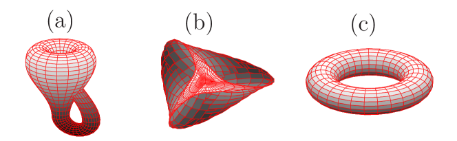
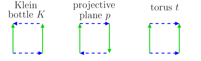
Figure 1: Top row: two-dimensional representations of (a) the Klein bottle $K$; of (b) the real projective plane $p$ (known also as the Roman surface or Steiner surface Steiner ); of (c) the torus $t$, all immersed in the three-dimensional $(x,y,z)$ space (see Fig. 2). The gray-scale code for surface facets denotes the position of the facet in z direction. Red lines denote the positions of the constant parameters for the surface parameterization. In order to produce these surfaces, the corresponding blue and green edges of a square should be “glued” together with the arrows matching (bottom row). Dashed blue lines and solid green lines represent the opposing boundaries.

Our goal is to study the thermodynamic properties of the Ising model on two-dimensional lattices which exhibit distinct topologies. Some of these topologies can be obtained from a square or a (rectangularly) shaped lattice by “glueing” opposite edges such that their orientations are parallel. We plot the Klein bottle, the real projective plane, and the torus in the first row of Figs. 1(a), (b), and (c), respectively. The directions, in which opposite sides of a rectangular lattice should be glued in order to produce such topologies, are presented in the second row of this figure. In turn, the polygon subjected to the glueing (of square or rectangular shape) may have different decorations (i.e., site positions and bond arrangements). In Fig. 2 we plot examples of triangular, square, and hexagonal decorations. We distinguish between the lattice type (triangular, square, hexagonal) and the lattice shape (rectangular or square). On the triangular lattice (tri., $\triangle$) each spin has six bonds, on the square lattice (sq., $\square$) each spin has four bonds, and on the hexagonal lattice (hex., $\hexagon$ ) each spin has three bonds.

As a reference case we consider the Ising model defined on a two-dimensional rectangular lattice of the size $L_{1}\times L_{2}$ with periodic boundary conditions (i.e., a torus) having a certain bond arrangement (triangle, square, and hexagonal) with lattice spacing $a=1$. We measure the size of a lattice in terms of the number $L_{1}$ of spins in a row (horizontal layers) and by the number $L_{2}$ of vertical layers. We note that a square lattice of rectangular shape $L_{1}\times L_{2}$ has the geometrical size $aL_{1}\times aL_{2}$, whereas for a triangular lattice of size $N=L_{1}\times L_{2}$ the geometrical size is $aL_{1}\times\frac{\sqrt{3}}{2}aL_{2}$.

In accordance with finite-size scaling theory Barber ; Privman , for the square lattice with the square shape $L_{1}=L_{2}=L$ and with the total number $N=L^{2}$ of spins, the magnetic susceptibility can be expressed as $\chi(\beta,L)=L^{\gamma/\nu}{\mathcal{X}}(tL^{1/\nu})=N^{\gamma/(2\nu)}{\mathcal{X}}(tN^{1/(2\nu)}).$ $\mathcal{X}$ is the dimensionless magnetic susceptibility scaling function, $t=(T-T_{c})/T_{c}=(\beta_{c}-\beta)/\beta$ is the reduced temperature, and $\nu=1$ and $\gamma=7/4$ are the correlation length and the magnetic susceptibility critical exponents PV , respectively.

For the square lattice of rectangular shape with the aspect ratio $\rho=L_{1}/L_{2}\neq 1$, or with $L_{1}=\rho L_{2}=:\rho L$, the magnetic susceptibility can be expressed as

$$\chi(\beta,\rho L,L)=N^{\gamma/(2\nu)}{\mathcal{X}}(\tau,\rho),$$ (4)

Here, $N=L_{1}L_{2}=\rho L^{2}$ is the total number of spins and $\tau=tN^{1/(2\nu)}$ is the temperature scaling variable.

We shall also consider the regular triangular lattice and the regular hexagonal lattice with the aspect ratio $\rho=L_{1}/L_{2}$ close to the special value $r_{0}$. This value $r_{0}$ is equal to $\sqrt{3}/2$ for the regular triangular lattice and $\sqrt{3}$ for the regular hexagonal lattice. The reason for selecting these values of the aspect ratio is discussed in Appendix A. One finds that lattices with these aspect ratios (in terms of the number of spins) exhibit a square geometrical shape.

We shall use the following values for the critical amplitudes of the bulk correlation length as obtained from the second moment of the two-point correlation function in the region above the critical point: $\xi_{0}^{+}\simeq 0.525315$ for the triangular ($\triangle$) lattice, $\xi_{0}^{+}\simeq 0.56706$ for the square ($\square$) lattice, and $\xi_{0}^{+}\simeq 0.657331$ for the hexagonal ($\hexagon$) lattice BCG .

III Lattices and topologies

Topology of a polyhedra is classified in accordance with its Euler characteristic Flegg

$${\mathcal{K}}=N-E+F,$$ (5)

where $N$ is the number of vertices (spins), $E$ is the number of edges (bonds), and $F$ is the number of facets. Every convex polyhedron can be turned into a connected, simple, planar graph. In turn, each connected planar graph has the same Euler characteristic ${\mathcal{K}}=2$.

For a regular triangular lattice forming a torus (which cannot be turned into a connected planar graph), exactly six edges (bonds, $b=6$) meet at each vertex (here and later on we denote by the letter $b$ the number of bonds (edges). Each edge has two ends so that the total number of edges is $E=3N$. Each triangular facet contains 3 vertices and each vertex participates in 6 facets, so that the total number of facets is $F=6N/3=2N$. Therefore, the Euler characteristic of the torus is ${\mathcal{K}}_{\mathrm{torus}}=0$. We can form the torus by using the triangular decoration (see Fig. 2(a)) and by applying the appropriate boundary conditions from Fig. 1(c). The Klein bottle (with Euler characteristic ${\mathcal{K}}_{\mathrm{Klein}}=\mathcal{K}_{\mathrm{torus}}=0$) is constructed by glueing the edges along the directions shown in Fig. 1(a). The real projective plane (${\mathcal{K}}_{\mathrm{p.\;plane}}=1$) may be produced by glueing edges in opposite directions for both pairs of sides (see Fig. 1(b)). For the Klein bottle and the real projective plane Eq. (5) is not applicable, because these non-orientable surfaces cannot be realized in three-dimensional space without self-intersection.

There is an analogous procedure for the square lattice: we use the square decoration of the lattice (see Fig. 2(b)) and apply the appropriate glueing of opposite sides (see Fig. 1). In the case of the projective plane two pairs of sites in opposite corners form double bonds between them. The same procedure is valid for the hexagonal lattice: one glues opposite sides of the lattice with hexagonal facets (see Fig. 2(c)) in accordance with one of the orientations indicated in Fig. 1.

Now we turn to surfaces with spherical topology corresponding to the Euler characteristic ${\mathcal{K}}_{\mathrm{sphere}}=2$. If we denote $n_{b}$ as the number of vertices which give rise to exactly $b$ edges, one has for the total number of vertices $N=\sum\limits_{b}n_{b}$. Since the total number of edges is $E=\frac{1}{2}\sum\limits_{b}bn_{b}$ and the total number of triangular facets is $F=\frac{1}{3}\sum\limits_{b}bn_{b}$, we can rewrite Eq. (5) as

$${\mathcal{K}}=N-E+F=\sum\limits_{b}(1-b/6)n_{b}.$$ (6)

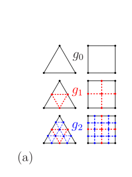
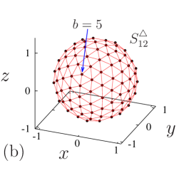
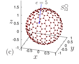
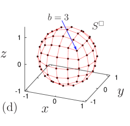
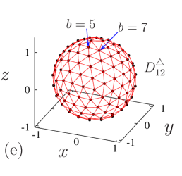
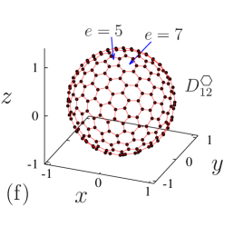
Figure 3: Structure of lattices with spherical geometry ($S$): (a) Recursive triangulation of a single triangular facet: the initial facet for the zeroth generation ($g_{0}$, solid line), the first ($g_{1}$, dashed line), and the second ($g_{2}$, dash-dotted line) generation. (b) Regular triangulation of the sphere ($S^{\triangle}_{12}$) with $n_{5}=12$ defects of type $b=5$ and $N=162$ (one defect $b=5$ is indicated by the blue arrow). (c) Regular decoration of the sphere by hexagons ($S^{\hexagon}_{12}$) with $n_{5}=12$ defects of type $e=5$, where $e$ denotes the number of edges, and $N=320$ (one defect $e=5$ is indicated). (d) Spherical representation of the surface of a cube with a regular square lattice ($S^{\square}$, see Table II) with $n_{3}=8$ defects of type $b=3$ (corners) and $N=98$ (one defect $b=3$ is indicated). (e) Random triangulation of the sphere ($D^{\triangle}_{12}$) with $n_{5}=16$ defects of type $b=5$ and $n_{7}=4$ defects of type $b=7$ and $N=162$ (two defects $b=7$ and $b=5$ are indicated). (f) Random representation of the sphere by hexagons ($D^{\hexagon}_{12}$, dual to $D^{\triangle}_{12}$) with $n_{5}=16$ defects of type $e=5$ and $n_{7}=4$ defects of type $e=7$ and $N=320$. The new bond on the dual lattice is perpendicular to the corresponding bond on the original lattice, i.e., a vertex is transformed into a facet and vice versa. For example, the defect vertex with $b=5$ bonds is transformed into the defect pentagon facet with $e=5$ edges (two defects $e=7$ and $e=5$, which correspond to panel (e), are indicated).

From this expression it follows that for spherical surfaces the regular triangulation, i.e., by a lattice of vertices which participate in six-bonds (i.e., $b=6$) vertices, as used for the surface of a torus, is not possible. For a sphere one needs a fraction of vertices with the associated number of bonds less than $6$, in accordance with Eq. (6) and with $\mathcal{K}=2$: $\sum\limits_{b}(6-b)n_{b}=12$; for example, $n_{5}=12$ vertices with $b=5$ bonds, $n_{4}=6$ vertices with $b=4$ bonds etc. We can construct the regular triangulation of a sphere in the following way. We start with a regular seed polyhedron with triangular facets (tetrahedron, octahedron, or icosahedron) and a circumscribed sphere of unit radius as a zero generation $k=0$ of our triangulation. In the next step, we add new vertices in the middle of each edge and connect these new vertices by new edges in order to create a generation $g_{1}$ (see Fig. 3(a)). The initial facet for the zero generation $g_{0}$ is a triangle. After this starting procedure, each triangle facet is split into four new facets of triangular shape $g_{1}$. Each new vertex is linked to exactly $b=6$ edges. After each iteration step we project the coordinates of the vertices of the next generation onto the surface of a unit sphere. After that we continue with the second iteration $g_{2}$, and so on. The number of vertices $N(k)$ for the $k$-th iteration step depends on the type of the polyhedron. We repeat this procedure until the desired level of triangulation is achieved. Because this recursive procedure generates only vertices with $b=6$, each triangulation inherits the number of defects from the seed polyhedron. The triangulation, which starts from a tetrahedron ( denoted as $S^{\triangle}_{4}$; here and in the following the subscript indicates the number of vertices of the seed polyhedron, and $S$ stands for sphere), has $n_{3}=4$ defects with $b=3$ bonds and has $N_{\mathrm{tet.}}(k)=4+2(4^{k}-1)$ vertices in the $k$-th step of the iteration. The triangulation, which starts from an octahedron ( denoted as $S^{\triangle}_{6}$) has $n_{4}=6$ defects with $b=4$ bonds and has $N_{\mathrm{oct.}}(k)=6+4(4^{k}-1)$ vertices in the $k$-th step of the iteration. Another regular triangulation, which starts from an icosahedron (denoted as $S^{\triangle}_{12}$) has $n_{5}=12$ defects with $b=5$ bonds and has $N_{\mathrm{icos.}}(k)=12+10(4^{k}-1)$ vertices in the $k$-th step. The latter version of triangulation is expected to be more homogeneous due to the small degree $(6-b)$ of defects, which leads to a higher level of symmetry. In Fig. 3(b) we plot the generation $k=2$ of the $S^{\triangle}_{12}$ triangulation, which contains $N=162$ vertices. One of the $b=5$ defects is indicated by an arrow.

Table 1: Structure of regular decorations of a sphere: number of vertices $N(k)$, edges $E(k)$, and facets $F(k)$ for the $k$-th generation of triangulations $\triangle$, which started from a tetrahedron, an octahedron, and an icosahedron. The square decoration $\square$ starts from a cube, and the hexagonal decoration $\hexagon$ is obtained as being dual to the triangular lattice for the icosahedron.

seed polyhedron	facet	gen.	$N(k)$	$E(k)$	$F(k)$
tetrahedron	$\triangle$	k	$4+2(4^{k}-1)$	$6\times 4^{k}$	$4\times 4^{k}$
octahedron	$\triangle$	k	$6+4(4^{k}-1)$	$12\times 4^{k}$	$8\times 4^{k}$
icosahedron	$\triangle$	k	$12+10(4^{k}-1)$	$30\times 4^{k}$	$20\times 4^{k}$
cube	$\square$	k	$2+6\times 4^{k}$	$12\times 4^{k}$	$6\times 4^{k}$
dual to icosahedron	$\hexagon$	k	$20\times 4^{k}$	$30\times 4^{k}$	$12+10(4^{k}-1)$

The regular decoration of a sphere by hexagons $S^{\hexagon}_{12}$ is constructed as a dual lattice for the triangular decoration, i.e., in the dual hexagonal lattice, each vertex corresponds to the triangular facet of the seed lattice and has exactly three edges. Defects of the seed lattice are transformed into facets, which are not hexagons. In Fig. 3(c) we plot the decoration by hexagons which is dual to the triangular decoration shown in Fig. 3(b). The defect with five edges ($b=5$) is transformed into a defect pentagonal facet denoted by $e$ with $e=5$.

For the square lattice we repeat the same procedure, using the cube as a seed polyhedron. In the first step, every square facet $g_{0}$ of a cube is split into four squares $g_{1}$ by adding new vertices and edges (see Fig. 3(a)). In the next step, each of the previously generated $g_{1}$ facets is split into four new facets $g_{2}$ and so on. After each iteration step we project the new vertices onto the unit sphere. This way we obtain a “sphero-cube” $S^{\square}$, i.e., a surface with spherical topology decorated by square facets as done in Ref. HL . This object has $n_{3}=4$ defects with $b=3$ bonds. The number of vertices in the $k$-th step is $N_{\mathrm{cube}}(k)=2+6\times 4^{k}$. In Fig. 3(d) we plot the “sphero-cube” with $N=98$ for the generation $k=2$; one of the $b=3$ defects is indicated by an arrow. The structure of regular decorations of a sphere is summarized in Table 1.

Table 2: List of the studied geometries for triangular (tri., $\triangle$), square (sq., $\square$), and hexagonal (hex., $\hexagon$) decorated lattices. Symbols for the notations, Euler characteristic $\mathcal{K}$, geometries, and brief descriptions (boundary conditions bc; random triangulation of the sphere $D^{\triangle}_{12}$.)

type	sym.	$\mathcal{K}$	geometry	description
tri.	$T^{\triangle}$	0	torus	triangular lattice with toroidal bc
tri.	$T^{\triangle}_{d}$	0	torus	triangular lattice with defects, toroidal bc
tri.	$T^{\triangle}_{r}$	0	torus	triangular lattice with defects, toroidal bc
tri.	$K^{\triangle}$	0	Klein bottle	triangular lattice with Klein bottle bc
tri.	$P^{\triangle}$	1	projective plane	triangular lattice with real projective plane bc
tri.	$S^{\triangle}_{12}$	2	sphere	triangulation of the sphere with $n_{5}=12$ defects
tri.	$S^{\triangle}_{6}$	2	sphere	triangulation of the sphere with $n_{4}=6$ defects
tri.	$S^{\triangle}_{4}$	2	sphere	triangulation of the sphere with $n_{3}=4$ defects
tri.	$D^{\triangle}_{12}$	2	sphere	dynamic triangulation of the sphere
sq.	$T^{\square}$	0	torus	square lattice with toroidal bc
sq.	$K^{\square}$	0	Klein bottle	square lattice with Klein bottle bc
sq.	$P^{\square}$	1	projective plane	square lattice with projective plane bc
sq.	$S^{\square}$	2	sphere	square lattice on the surface of the cube
hex.	$T^{\hexagon}$	0	torus	hexagonal lattice with toroidal bc
hex.	$K^{\hexagon}$	0	Klein bottle	hexagonal lattice with Klein bottle bc
hex.	$P^{\hexagon}$	1	projective plane	hexagonal lattice with real projective plane bc
hex.	$S^{\hexagon}_{12}$	2	sphere	hexagonal decoration of a sphere (dual to $S^{\triangle}_{12}$)
hex.	$D^{\hexagon}_{12}$	2	sphere	hexagonal decoration of a sphere (dual to $D^{\triangle}_{12}$)

From a very simplified point of view the sphere triangulation $S^{\triangle}_{12}$ is the lattice in which 12 vertices have $b=5$ bonds and all remaining vertices have $b=6$ bonds. It is interesting to see whether differences in the results obtained for triangular toroidal lattices (defect-free) and for spherical lattices (with defects) are due to these defects. In order to clarify this point we consider a toroidal triangular lattice with 6 removed bonds (defects). The presence of those defects produces 12 vertices with $b=5$ bonds (like for the sphere triangulation $S^{\triangle}_{12}$). We consider the case, in which these defect bonds are regularly distributed in order to have maximal separation between them (we denote this case as $T^{\triangle}_{d}$) (Fig. 2(d)). The case, in which these defect bonds are randomly distributed over the lattice, is denoted as $T^{\triangle}_{r}$.

We have also studied a random (dynamic) triangulation of the sphere. In order to create a configuration with random positions of the vertices, we implement Langevin dynamics for $N$ particles on a sphere with mutual pairwise repulsion. Having the vertices randomly distributed, we apply Delaunay triangulation Delaunay ; DelProg . (This procedure is described in full details in Ref. VMD ; therefore we refrain to repeat it here.) The number of particles ( i.e., vertices) is chosen as for the regular triangulation $S^{\triangle}_{12}$. Accordingly, we denote the results for this dynamic triangulation as $D^{\triangle}_{12}$. An example of the random triangulation of the sphere with $N=162$ vertices (spins) is shown in Fig. 3(e). This realization encompasses $n_{5}=16$ defects of type $b=5$ and $n_{7}=4$ defects of type $b=7$. Two of these defects ($b=7$ and $b=5$) are indicated in the figure. An example of hexagonal decoration (dual to the lattice in Fig. 3(e)) is provided in Fig. 3(f). Here pentagon $e=5$ and heptagon $e=7$ facets correspond to $b=5$ and $b=7$ defects in Fig. 3(e). Notations and brief descriptions for the considered geometries are collected in Table 2.

IV Simulation results

We use Monte Carlo (MC) simulations LB to compute the specific heat $C$ and the magnetic susceptibility $\chi$ in accordance with Eqs. (2) and (3), respectively, for various lattices with distinct topologies. Our aim is to determine the finite size scaling functions of these quantities near the bulk critical point of the two-dimensional Ising model. The specific heat $C$ and the magnetic susceptibility $\chi$ are second derivatives of the free energy, and at the critical point they diverge as the system size (i.e., the number of spins $N$) tends to infinity $N\to\infty$, i.e., $C\propto\ln(N)$ and $\chi\propto N^{7/8}$. (The critical scaling of the specific heat is discussed in Appendix B). Quantities like the mean magnetization $\left<|M|\right>/N$ and the mean energy $\langle U\rangle/N$ per site, which can be easily inferred from the MC simulations, are not very informative, because they remain finite at the critical point.

Before starting the numerical measurements, we allow the system to thermalize, using $5\times 10^{6}$ (MC) steps. Then we perform the thermal average of the thermodynamic quantities over $10^{7}$ (MC) steps, split into 10 series of $10^{6}$ steps in order to determine the numerical error. Each MC step consists of a cluster update in accordance with the Wolff algorithm Wolff . We mainly focus on the triangular lattice decoration, because triangulation is a common method for the grid representation of surfaces. We use the temperature scaling variable $x=\tau/(\xi_{0}^{+})^{1/\nu}=t(N^{1/2}/\xi_{0}^{+})^{1/\nu}$, where the numerical values of the bulk correlation length amplitudes $\xi_{0}^{+}$ are provided in Sec. II. We note that in the special case of a square decoration of the lattice, which is shaped as a square $N=L\times L$, this scaling variable equals $x=(L/\xi)^{1/\nu}$.

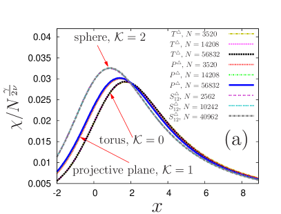
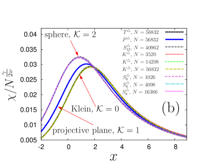
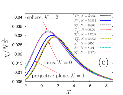
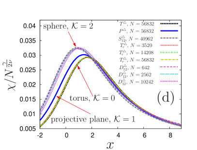
Figure 4: Rescaled magnetic susceptibility $\chi/N^{\gamma/(2\nu)}$ for triangular lattice decorations as a function of the scaling variable $x=t(N^{1/2}/\xi_{0}^{+})^{1/\nu}$ for various topologies (the reference curves are $T^{\triangle}$ and $P^{\triangle}$ for $N=56832$ and $S^{\triangle}_{12}$ for $N=40962$, which are reproduced in all panels): (a) torus ($T^{\triangle}$), real projective plane ($P^{\triangle}$), and regular triangulation of a sphere with $n_{5}=12$ defects ($S^{\triangle}_{12}$); (b) reference curves, curves for the Klein bottle ($K^{\triangle}$), and curves for the regular triangulation of a sphere with $n_{4}=6$ defects ($S^{\triangle}_{6}$); (c) reference curves, curves for the torus with regularly distributed defects denoted by subscript $d$ ($T^{\triangle}_{d}$), and curves for the regular triangulation of a sphere with $n_{3}=4$ defects ($S^{\triangle}_{4}$); (d) reference curves, curves for the torus with randomly distributed defects denoted by subscript $r$ ($T^{\triangle}_{r}$), and curves for the random triangulation of a sphere with the number of particles as for $n_{5}=12$ defects ($D^{\triangle}_{12}$).

In Fig. 4 we plot the rescaled magnetic susceptibility in terms of the magnetic susceptibility scaling function ${\mathcal{X}}=\chi/N^{\gamma/(2\nu)}$ as function of the temperature scaling variable $x$ for the triangular ($\triangle$) lattice, forming surfaces with different topologies and for several numbers of spins $N$. As master curves we select the regular toroidal geometry ($T^{\triangle}$) with $N=56832$ spins (dashed line), the real projective plane geometry ($P^{\triangle}$) with $N=56832$ spins (solid line), and the regular sphere triangulation ($S^{\triangle}_{12}$) with $N=40962$ spins (dash-dotted line). As a reference, these master curves are included in all panels.

For completeness, in Fig. 4(a) we reproduce our results from Ref. VMD , which allows us to compare the regular toroidal geometry ($T^{\triangle}$), the projective plane geometry ($P^{\triangle}$), and the regular triangulation of the sphere with icosahedron symmetry ($S^{\triangle}_{12}$). In Fig. 4(b) we focus on the comparison of the Klein bottle ($K^{\triangle}$) with the regular triangulation of the sphere with octahedron symmetry ($S^{\triangle}_{6}$). In Fig. 4(c), the toroidal geometry with equidistant defects ($T_{d}$) is compared with the regular triangulation of a sphere with tetrahedron symmetry ($S^{\triangle}_{4}$). Finally, in Fig. 4(d) we compare the torus with randomly distributed defects ($T_{r}$) and the sphere ($D^{\triangle}_{12}$) with random triangulation. We find, that the magnetic susceptibility always falls onto master curves defined by the Euler characteristic.

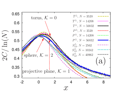
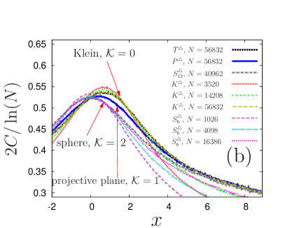
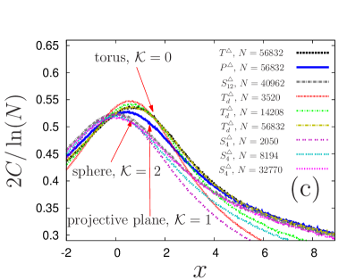
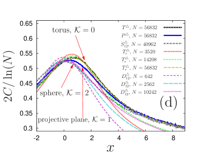
Figure 5: Rescaled specific heat $2C/\ln(N)$ for triangular lattice decorations as function of the scaling variable $x=t(N^{1/2}/\xi_{0}^{+})^{1/\nu}$ for various types of topologies ( the reference curves are $T^{\triangle}$ and $P^{\triangle}$ for $N=56832$ and $S^{\triangle}_{12}$ for $N=40962$): (a) torus ($T^{\triangle}$), real projective plane ($P^{\triangle}$), and regular triangulation of a sphere with $n_{5}=12$ defects ($S^{\triangle}_{12}$); (b) reference curves, Klein bottle ($K^{\triangle}$), and regular triangulation of a sphere with $n_{4}=6$ defects ($S^{\triangle}_{6}$); (c) reference curves, torus with regularly distributed defects ($T^{\triangle}_{d}$), and regular triangulation of a sphere with $n_{3}=4$ defects ($S^{\triangle}_{4}$); (d) reference curves, torus with randomly distributed defects ($T^{\triangle}_{r}$), and random triangulation of a sphere with the number of particles as for $n_{5}=12$ defects ($D^{\triangle}_{12}$).

In Figs. 5(a), (b), (c), and (d) we show the rescaled specific heat $2C/\ln(N)$ as a function of the scaling variable $x$ for a triangular lattice and for the same geometries as in Figs. 4(a), (b), (c), and (d), respectively. We observe that, unlike the magnetic susceptibility, the specific heat does not ideally fall into a set of master curves. This could be due to large finite size corrections to the logarithmic scaling and due to the contribution of the regular part $C(\beta,N)\simeq C_{\mathrm{reg}}+{\mathcal{C}}(x)\ln(N)/2$, which defines the scaling function ${\mathcal{C}}(x)$ (see Appendix B for additional details). Nonetheless one can clearly identify three branches of curves which correspond to systems with different values of the Euler characteristic $\mathcal{K}=0,1,2$. But the order of the curves is opposite to that for the magnetic susceptibility: upon increasing the Euler characteristic the function $2C/\ln(N)$ shifts to lower values and its maximum moves to smaller values of the scaling variable $x$; the curves from top to bottom in Fig. 5 correspond to the torus and the Klein bottle, to the projective plane, and to the sphere. For the curves in Fig. 4 the opposite holds.

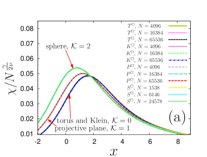
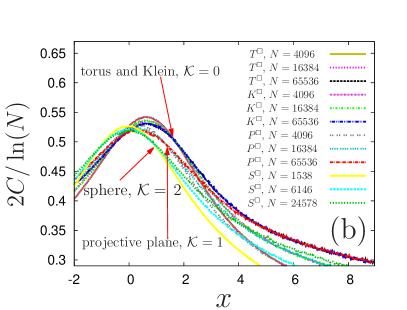
Figure 6: Simulation results for square lattice decorations with various topologies: torus ($T^{\square}$), Klein bottle ($K^{\square}$), real projective plane ($P^{\square}$), and deformed cube surface ($S^{\square}$). (a) Rescaled magnetic susceptibility $\chi/N^{\gamma/(2\nu)}$ and (b) rescaled specific heat $2C/\ln(N)$ as function of the scaling variable $x=t(N^{1/2}/\xi_{0}^{+})^{1/\nu}$.

Again for completeness, in Fig. 6(a) we reproduce results from Ref. VMD for the magnetic susceptibility scaling function for the square lattice decoration with various topologies and system sizes. As for the triangular lattice, we observe a perfect data collapse for the surfaces with the same value of the Euler characteristic $\mathcal{K}$.

The specific heat for the square lattice and for various topologies is shown in Fig. 6(b). It behaves in the same way as the specific heat for the triangular decorations.

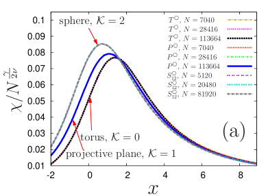
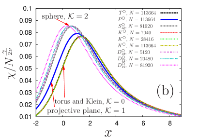
Figure 7: Rescaled magnetic susceptibility $\chi/N^{\gamma/(2\nu)}$ for hexagonal lattice decorations as function of the scaling variable $x=t(N^{1/2}/\xi_{0}^{+})^{1/\nu}$ and for various topologies. The reference curves are $T^{\hexagon}$ and $P^{\hexagon}$ for $N=113664$ and $S^{\hexagon}_{12}$ for $N=81920$. (a) Torus ($T^{\hexagon}$), real projective plane ($P^{\hexagon}$), and sphere ($S^{\hexagon}_{12}$, dual to $S^{\triangle}_{12}$); (b) reference curves, Klein bottle ($K^{\hexagon}$), and random representation of a sphere ($D^{\hexagon}_{12}$ dual to $D^{\triangle}_{12}$).

In Fig. 7 we present simulation results for the magnetic susceptibility in the case of a lattice with hexagonal decoration. The simulation results for the regular torus ($T^{\hexagon})$, the real projective plane ($P^{\hexagon}$), and the sphere $S^{\hexagon}_{12}$ (dual to $S^{\triangle}_{12}$) are presented in Fig. 7(a). Finally, in Fig. 7(b) we compare the master curves from Fig. 7(a) with the results for the Klein bottle $K^{\hexagon}$ and the dynamic configuration $D^{\hexagon}_{12}$ (which is dual to the dynamic triangulations $D^{\triangle}_{12}$).

In sum, we find the same feature as for the other decorations: the curves split into three branches which correspond to three different values of the topological characteristic, i.e., $\mathcal{K}=0,1,2$. The results for the torus and for the Klein bottle belong to the same branch.

V Conclusions

We have numerically investigated the dependence of thermodynamic functions of the two-dimensional Ising model on the topology of its surfaces. We have studied lattices with triangular, square, and hexagonal facets. These lattices have the topology of a torus (Euler characteristic $\mathcal{K}=0$), a Klein bottle ($\mathcal{K}=0$), a real projective plane ($\mathcal{K}=1$), and a sphere ($\mathcal{K}=2$), respectively. We find, that the magnetic susceptibility scaling function splits into distinct branches of curves in accordance with the topology classes of the surfaces. For each type of the lattice tiling and within the same topological class (i.e., the same value of the Euler characteristic $\mathcal{K}$) the curves exhibit excellent data collapse, while for different topological classes the curves differ from each other. There are differences between the shapes of the scaling functions for the same topology but different lattice tiling. Importantly, we have found that also the scaling function of the specific heat depends on the topological class of the surface. Although in this case the data collapse is much worse, we can firmly state that there is a similar splitting into branches associated with the value of $\mathcal{K}$.

A natural but challenging extension of the present research would be off-lattice simulations using, for example, molecular dynamics methods. This would allow one to address the issue of universality for systems confined to surfaces with different topologies. It is unclear to which extent the universal properties of the critical demixing transition of binary liquid mixtures are shared by the two-dimensional Ising model if the surfaces of these systems are nonplanar.

Appendix A Aspect ratio dependence and finite size scaling for the magnetic succeptibility

The general form of the aspect ratio dependence of the percolation function $\pi_{h}(\rho)$ (i.e., the probability to have a percolating cluster in the horizontal direction) has been presented by Langlands et al. LPPS . We note that the percolation temperature of so-called physical clusters in the 2D Ising model with vanishing bulk ordering field coincides with the critical temperature $T_{c}$. Therefore the percolation probability behaves in a way very similar to the spontaneous magnetization CNPR . For each type of the lattice, there exists a special, so-called “reference” value $r_{0}$ of the aspect ratio $\rho=L_{1}/L_{2}$, which captures the geometrical size of the lattice. Leglands showed that if one measures the aspect ratio $\rho$ in units of $r_{0}$, i.e., if one writes $\rho=rr_{0}$ where $r\equiv(L_{1}/L_{2})/r_{0}$, the crossing probability as a function of $\rho$ may be written as

$$\pi_{h}(rr_{0})=\eta_{h}(r)$$ (7)

where $\eta_{h}(r)=\eta_{h}(1/r)$ is a universal function (which is self-dual with respect to its argument $r\to 1/r$). The values of this reference aspect ratio for triangular, square, and hexagonal lattices are $r_{0}=\sqrt{3}/2,1,$ and $\sqrt{3}$, respectively. We recall, that the system sizes $L_{1}$ and $L_{2}$ are measured in numbers of spins in the rows and the columns, respectively. The result in Eq. (7) implies, that for the comparison of the scaling functions for different types of lattices, one should choose $L_{1}$ and $L_{2}$ such that the geometrical sizes of these lattices are equal. In view of Eq. (7) we expect that Eq. (4) may be written for various lattice types as

$$\chi(\beta,rr_{0}L,L)=N^{\frac{\gamma}{2\nu}}{\mathcal{X}}(\tau,r),$$ (8)

where the scaling function ${\mathcal{X}}$ is dual with respect to its second argument: ${\mathcal{X}}(\tau,r)={\mathcal{X}}(\tau,1/r)$.

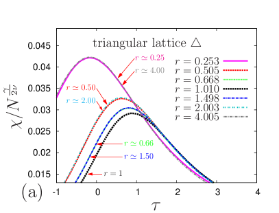
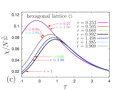
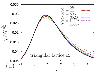
Figure 9: Rescaled magnetic susceptibility $\chi/N^{\gamma/(2\nu)}$ as function of the temperature scaling variable $\tau=tN^{1/(2\nu)}$. (The temperature scaling variable $x$ includes the correlation length amplitude $\xi_{0}^{+}$, the variable $\tau$ does not include it: $x=\tau(\xi_{0}^{+})^{-1/\nu}$.) The data correspond to the toroidal topology with various values of the reduced aspect ratio $r=\rho/r_{0}$: (a) on the triangular lattice; (b) on the square lattice; (c) on the hexagonal lattice. (d) Rescaled magnetic susceptibility $\chi/N^{\gamma/(2\nu)}$ as function of the scaling variable $\tau=tN^{1/(2\nu)}$ on the triangular lattice (i.e., the toroidal topology) for various numbers of spins: $N=56,224,896,3520,14208$, and $56832$; the aspect ratio is $\rho\simeq r_{0}=\frac{\sqrt{3}}{2}$. For further information see the main text in Appendix A.

We have checked Eq. (8) numerically and present the corresponding results in Fig. 9. In this figure we plot the rescaled magnetic susceptibility ${\mathcal{X}}=\chi/N^{\gamma/(2\nu)}$ as function of the temperature scaling variable $\tau=tN^{1/(2\nu)}$ for triangular [Figs. 9(a) and 2(a)], square [Figs. 9(b) and 2(b)], and hexagonal [Figs. 9(c) and 2(c)] lattices. These lattices have a rectangular shape of width $L_{1}=64$ and periodic boundary conditions (i.e., toroidal geometry). The considered values of the reduced aspect ratio $r=\rho/r_{0}$ (i.e., $\rho$ in units of $r_{0}$) are $r=0.25,0.5,0.6\bar{6},1,1.5,2,$ and $4$. The length of the lattice $L_{1}\simeq\rho L_{2}=rr_{0}L_{2}$ is chosen as the integer closest to the number $rr_{0}L_{2}$. In every panel we plot the magnetic susceptibility for the self-dual ratio $r\simeq 1$ and for a set of dual values $r$ and $r^{\prime}\simeq 1/r$. (In the general case it is impossible to realize the equality $r^{\prime}=1/r$ because both $L_{1}$ and $L_{2}$ are integer.) Upon increasing the reduced aspect ratio $r$, the position $\tau_{\mathrm{max}}$ of the maximum of $\chi/N^{\gamma/(2\nu)}$ as a function of $r$ shifts to larger values of $\tau$. This occurs up to the self-dual value $r=1/r=1$. Upon increasing $r$ further, the position of the maximum shifts back to lower values of $\tau$. We observe that the values of $\chi/N^{\gamma/(2\nu)}$ for $r$ and $r^{\prime}\simeq 1/r$ coincide in accordance with our expectation that ${\mathcal{X}}(\tau,r)={\mathcal{X}}(\tau,1/r)$. Thus, for the triangular and the hexagonal lattice we should use the aspect ratio, which is a multiple of the reference value $r_{0}=\sqrt{3}/2\quad\simeq 0.86602$ and $r_{0}=\sqrt{3}\quad\simeq 1.73205$, respectively, and which corresponds to the square geometry on the square lattice.

In Fig. 9(d) we plot the rescaled magnetic susceptibility $\chi/N^{\gamma/2\nu}$ as a function of the scaling variable $\tau=tN^{1/(2\nu)}$ on the triangular lattice with the selected aspect ratio $\rho\simeq r_{0}=\sqrt{3}/2$ for various numbers of spins: $N=56,224,896,3520,14208,\mathrm{and}\quad 56832$. We observe noticeable finite size corrections to scaling for lattices of small sizes ($N<1000$) while for larger system sizes the curves coincide. Therefore it is preferable to use large lattices ($N>1000$) in order to avoid corrections to scaling and to observe good data collapse.

Appendix B Finite size scaling for the specific heat

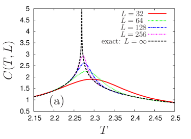
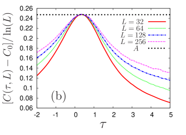
Figure 10: (a) Specific heat $C(T,L)$ as function of the temperature $T$ for four lattice sizes $L=32,64,128,256$ in comparison with the exact result in Eq. (9). (b) Rescaled specific heat $(C-C_{0})/\ln(L)$ as function of $\tau=tL$ compared with the maximum value $A$. For further information see the main text in Appendix B.

The singular part of the specific heat of the Ising model on the two-dimensional lattice exhibits a logarithmic divergence. In Fig. 10(a) we compare numerical results for the specific heat $C$ as function of temperature $T$ (in units of the coupling constant $J$) on square lattices of sizes $L=32,64,128,$ and $256$ for the toroidal geometry with the analytic expression MW

$$C(T\to T_{c})\simeq\frac{8}{\pi T_{c}^{2}}\left[\ln\left|\frac{\sqrt{2}}{\frac{1}{T}-\frac{1}{T_{c}}}\right|-(1+\pi/4)\right]$$ (9)

Concerning the maximum of the specific heat for finite $L$ one has $C_{\mathrm{max}}(L)\simeq A\ln(L)+C_{0}$ where $A=\frac{4}{\pi T_{c}^{2}}$ and $C_{0}\simeq 0.1879\frac{1}{T_{c}^{2}}$. In Fig. 10(b) we plot the rescaled specific heat $[C-C_{0}]/\ln(L)$ as function of the scaling variable $\tau=tL$ in comparison with $A$. We find, that after this rescaling all maxima coincide and correspond to the expected value $A$. However, in Fig. 10(b) the curves differ from each other and it is impossible to bring them on top of each other by rescaling the axis $\tau$. The issue of how to rescale the specific heat with the logarithm $\ln(L)$ of the system size, in order to obtain data collapse, remains open. We have decided to scale our results for the specific heat as $C/\ln(L)=2C/\ln(N)$, where the total number $N$ of spins for the square lattice is $N=L^{2}$. The aspect ratio dependence of the specific heat of the Ising model on the square lattice of rectangular shape has been studied in Ref. FF .

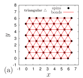
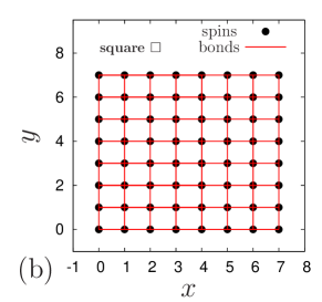
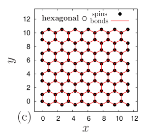
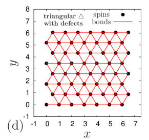
Figure 2: Decorations of lattices: (a) regular triangular lattice ($\triangle$) of size $7\times 8$, i.e., $N=56$; (b) regular square lattice ($\square$) of size $8\times 8$, i.e., $N=64$; (c) regular hexagonal lattice ($\hexagon$) of size $14\times 8$, i.e., $N=112$; (d) triangular lattice ($\triangle$) with 12 defects of type $b=5$ (i.e., 6 missing bonds) of size $7\times 8$, i.e., $N=56$.

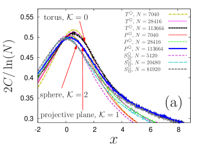
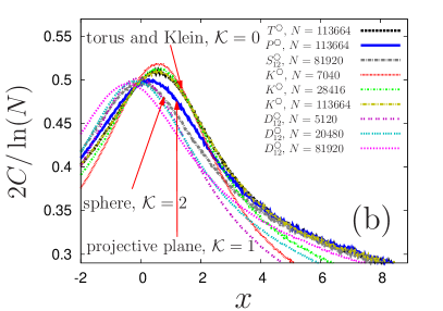
Figure 8: Rescaled specific heat $2C/\ln(N)$ for hexagonal lattice decorations as function of the scaling variable $x=t(N^{1/2}/\xi_{0}^{+})^{1/\nu}$ and for various topologies. The reference curves are $T^{\hexagon}$ and $P^{\hexagon}$ for $N=113664$ and $S^{\hexagon}_{12}$ for $N=81920$. (a) Torus ($T^{\hexagon}$), real projective plane ($P^{\hexagon}$), and sphere ($S^{\hexagon}_{12}$, dual to $S^{\triangle}_{12}$); (b) reference curves, Klein bottle ($K^{\hexagon}$), and random representation of a sphere ($D^{\hexagon}_{12}$ dual to $D^{\triangle}_{12}$).

References

- (1) V. V. Moshchalkov, L. Gielen, C. Strunk, R. Jonckheeret, X. Qiu, C. Van Haesendonck, and Y. Bruynseraede, Effect of sample topology on the critical fields of mesoscopic superconductors, Nat. 373, 319 (1995).
- (2) D. Makarov, O. M. Volkov, A. Kákay, O. V. Pylypovskyi, B. Budinská, and O. V. Dobrovolskiy, New Dimension in Magnetism and Superconductivity: 3D and Curvilinear Nanoarchitectures, Adv. Mater. 34, 2101758 (2020).
- (3) O. V. Dobrovolskiy, O. V. Pylypovskyi, L. Skoric, A. Fernández-Pacheco, A. Van Den Berg, S. Ladak, and M. Huth, Complex-Shaped 3D Nanoarchitectures for Magnetism and Superconductivity in Curvilinear Micromagnetism: From Fundamentals to Applications edited by D. Makarov and D. D. Sheka (Springer International Publishing, Cham, 2022) p. 215–268.
- (4) S. Tanda, T. Tsuneta, Y. Okajima, K. Inagaki, K. Yamaya, and N. Hatakenaka, A Möbius strip of single crystals, Nat. 417, 397 (2002).
- (5) Z. Geng, B. Xiong, K. Wang, M. Ren, L. Zhang, J. Zhu, and Z. Yang, Möbius strips of chiral block copolymers, Nat. Commun. 10, 4090 (2019).
- (6) G. Ouyang, L. Ji, Y. Jiang, F. Würthner, M. Liuet, Self-assembled Möbius strips with controlled helicity, Nat. Commun 11, 5910 (2020).
- (7) S.L. Veatch, P. Cicuta, P. Sengupta, A. Honerkamp-Smith, D. Holowka, and B. Baird, Critical fluctuations in plasma membrane vesicles, ACS Chem. Biol. 3, 287 (2008).
- (8) E. Gray, J. Karslake, B.B. Machta, and S.L. Veatch, Liquid general anesthetics lower critical temperatures in plasma membrane vesicles, Biophys. J. 105, 2751 (2013).
- (9) O.V. Pylypovskyi, V.P. Kravchuk, D.D. Sheka, D. Makarov, O.G. Schmidt, and Y. Gaididei, Coupling of Chiralities in Spin and Physical Spaces: The Möbius Ring as a Case Study , Phys. Rev. Lett. 114, 197204 (2015).
- (10) O.A. Vasilyev, A. Maciolek and S. Dietrich, Criticality senses topology, EPL 128, 20002 (2019).
- (11) K. Kaneda and Y. Okabe, Finite-size scaling for the Ising model on the Möbius strip and the Klein bottle, Phys. Rev. Lett. 86, 2134 (2001).
- (12) W.T. Lu and F.Y. Wu, Ising model on nonorientable surfaces: Exact solution for the Möbius strip and the Klein bottle, Phys. Rev. E 63, 026107 (2001).
- (13) C. Hoelbling and C.B. Lang, Universality of the Ising model on spherelike lattices, Phys. Rev. B 54, 3434 (1996).
- (14) D.P. Landau and K. Binder, A Guide to Monte Carlo Simulations in Statistical Physics (Cambridge University Press, London, 2005).
- (15) M. N. Barber, in Phase Transitions and Critical Phenomena, edited by C. Domb and J. L. Lebowitz (Academic, New York, 1983), Vol. 8, p. 149.
- (16) V. Privman, in Finite Size Scaling and Numerical Simulation of Statistical Systems, edited by V. Privman (World Scientific, Singapore, 1990), p. 1.
- (17) A Pelissetto and E Vicari, Critical phenomena and renormalization-group theory, Phys. Rep. 368, 549 (2002).
- (18) P. Butera, M. Comi, and A.J. Guttmann, Critical parameters and universal amplitude ratios of two-dimensional spin-S Ising models using high- and low-temperature expansions, Phys. Rev. B 67, 054402 (2003).
- (19) G. H. Flegg, From Geometry to Topology, (Dover Books on Mathematics, 2001).
- (20) D. W. Jacobsen, M. Gunzburger, T. Ringler, J. Burkardt, and J. Peterson, Parallel algorithms for planar and spherical Delaunay construction with an application to centroidal Voronoi tessellations, Geosci. Model 6, 1353 (2013).
-
(21)
The FORTRAN code for Delaunay triangulation of a sphere
is available (under GNU LGPL license)
on John Burkardt’s web-page
https://people.sc.fsu.edu/ jburkardt/f_src/
sphere_delaunay/sphere_delaunay.html - (22) U. Wolff, Collective Monte Carlo Updating for Spin Systems, Phys. Rev. Lett. 62, 361 (1989).
- (23) R.P. Langlands, C. Pichet, Ph. Pouliot, and Y. Saint-Aubin, On the universality of crossing probabilities in two-dimensional percolation, J. Stat. Phys. 67, 553 (1992).
- (24) A. Coniglio, C. R. Nappi, F. Peruggi, and L. Russo, Percolation points and critical point in the Ising model, J. Phys. A: Math. Gen. 10, 205 (1977).
- (25) B.M. McCoy and T.T. Wu, The two-dimensional Ising model, (Harvard Univ. Press, Cambridge, MA, 1973).
- (26) E. Ferdinand and M.E. Fisher, Bounded and inhomogeneous Ising models. I. Specific-heat anomaly of a finite lattice, Phys. Rev., 185 (1969) 832.
- (27) A. Coffman, A. Schwartz, and C. Stanton, The Algebra and Geometry of Steiner and Other Quadratically Parametrizable Surfaces, Computer Aided Geometric Design, 13, 257 (1996).