A model-free shrinking-dimer saddle dynamics for finding saddle point and solution landscape

Abstract

We propose a model-free shrinking-dimer saddle dynamics for finding any-index saddle points and constructing the solution landscapes, in which the force in the standard saddle dynamics is replaced by a surrogate model trained by the Gassian process learning. By this means, the exact form of the model is no longer necessary such that the saddle dynamics could be implemented based only on some observations of the force. This data-driven approach not only avoids the modeling procedure that could be difficult or inaccurate, but also significantly reduces the number of queries of the force that may be expensive or time-consuming. We accordingly develop a sequential learning saddle dynamics algorithm to perform a sequence of local saddle dynamics, in which the queries of the training samples and the update or retraining of the surrogate force are performed online and around the latent trajectory in order to improve the accuracy of the surrogate model and the value of each sampling. Numerical experiments are performed to demonstrate the effectiveness and efficiency of the proposed algorithm.

MSC Classification]37M05, 60G15, 65D15, 62L05

1 Introduction

Finding saddle points on complex energy landscapes or dynamical systems provides substantial physical and chemical properties and is thus an important problem in various fields such as nucleation and phase transformations in solid and soft matter ZhangChe ; ZhangCheDu and transition rates in chemical reactions and computational biology Nie2020 ; wang2021modeling ; Yin2020nucleation . The saddle points could be classified by the Morse index characterized by the maximal dimension of a subspace on which the Hessian $H(x)$ is negative definite Milnor . In practice, the index-1 saddle point represents the transition state connecting two local minima according to the transition state theory Mehta ; ZhaRen . The index-2 saddle points are particularly useful for providing trajectory information of chemical reactions in chemical systems Heidrich1986 . The excited states in quantum systems can also be characterized as saddle point configurations foresman1992toward .

There exist several algorithms of finding index-1 saddle points, e.g. EZho ; Gou ; ZhaDu . However, the computation of high-index (index$>1$) saddle point is more difficult as it has multiple unstable eigen-directions and receives less attention, though the number of high-index saddle points are much larger than the number of local minima and index-1 saddle points on the energy landscape Chen2004 ; Li2001 . High-index shrinking-dimer saddle dynamics proposed in YinSISC , which involves the force calculation (i.e. the negative gradient of the energy function), provides an effective means for finding any-index saddle points. This method is then combined with the downward search algorithm YinPRL ; YinSCM to construct the solution landscapes of both energy systems and dynamical (non-gradient) systems HanYin ; han2021a ; Luo2022 ; shi2022 . However, it is possible that the exact form of the force is not given a priori in some cases such that we need to either investigate the modeling of the underlying processes or perform experiments in order to obtain the inquired values of the force in saddle dynamics. In practice, modeling complex problems may be difficult or inaccurate, which often restricts the computation of the saddle points and its applications.

To resolve this issue, we employ a data-driven approach to propose a model-free saddle dynamics, in which the force in the original saddle dynamics is replaced by a surrogate model trained by the Gassian process learning. In the past few decades, the Gaussian process has been widely employed in extensive applications for constructing the surrogate models from the training data RaiPerKar ; RasWil . In particular, there exist some recent works on combining the Gaussian process with searching algorithms of index-1 saddle points Den ; GuWan ; KoiDag . Here we adopt this idea in the computation of high-index saddle points. By this means, the exact form of the model is no longer necessary such that the saddle dynamics could be implemented based only on some observations of the force. Furthermore, the number of the force calculations during training is generally smaller than that in performing the saddle dynamics.

Based on the proposed model-free saddle dynamics and its local nature, we adopt the sequential learning framework Pow to develop a sequential learning saddle dynamics algorithm in which the queries of the training samples and the update or retraining of the surrogate force are performed online and around the latent trajectory. In this way, the accuracy of the surrogate model and the value of each sampling could be improved such that the queries of the force could be further reduced. The proposed method could be further combined with the downward search algorithm for construction of the model-free solution landscape YinPRL ; YinSCM , which provides a pathway map consisting of both saddle points and minima and avoids the sampling on energy landscape of the model system. Numerical experiments are performed to demonstrate the effectiveness and efficiency of the proposed algorithm in comparison with the standard saddle dynamics.

The rest of the paper is organized as follows: In Section 2 we propose a model-free shrinking-dimer saddle dynamics by incorporating the Gaussian process learning with the original saddle dynamics. In Section 3 we present a sequential learning saddle dynamics algorithm to compute high-index saddle points and construct the solution landscapes. Numerical experiments are performed in Section 4 and we draw concluding remarks in the last section.

2 Model-free saddle dynamics

We present a model-free shrinking-dimer saddle dynamics for finding high-index saddle points of complex energy functions or dynamical systems, in which the exact form of the force may not be given a priori and is recovered from its observations at discrete locations. By this means, the saddle dynamics could be implemented based on these observations from, e.g., experiments or simulations, even without knowing the formulations of the energy functions or dynamics. This data-driven approach not only avoids the modeling procedure that could be difficult or inaccurate, but could significantly reduce the number of queries of the true force that may be expensive or time-consuming in practical problems.

2.1 Saddle dynamics and its implementation

We begin by introducing the high-index saddle dynamics proposed in YinSISC to find an index-$k$ ($1\leq k\in\mathbb{N}$) saddle point of an energy function $E(x)$

$$\left\{\begin{array}[]{l}\displaystyle\frac{dx}{dt}=\beta\bigg{(}I-2\sum_{j=1}^{k}v_{j}v_{j}^{\top}\bigg{)}F(x),\\[5.42003pt] \displaystyle\frac{dv_{i}}{dt}=\gamma\bigg{(}I-v_{i}v_{i}^{\top}-2\sum_{j=1}^{i-1}v_{j}v_{j}^{\top}\bigg{)}H(x)v_{i},~{}~{}1\leq i\leq k.\end{array}\right.$$ (1)

Here the force $F:\mathbb{R}^{N}\rightarrow\mathbb{R}^{N}$ is generated from the energy $E(x)$ by $F(x)=-\nabla E(x)$, $H(x):=-\nabla^{2}E(x)$ corresponds to the Hessian of $E(x)$, $\beta$, $\gamma>0$ are relaxation parameters, $x$ represents the state variable and direction variables $\{v_{i}\}_{i=1}^{k}$ form a basis for the unstable subspace of the Hessian at $x$.

More generally, (1) could be applied to find the saddle points of the dynamical systems $\dot{x}=F(x)$ which could be non-gradient, i.e., $F(x)$ is not a negative gradient of some energy function $E(x)$. In this case, the Hessian in (1) should be replaced by the Jacobian of $F(x)$ or its symmetrization YinSCM ; Z3 . Without loss of generality, we focus on the saddle dynamics of gradient systems in this paper.

As it is often expensive to calculate and store the Hessian, the dimer method HenJon ; ZhaDu ; ZhaSISC is applied to approximate the multiplication of the Hessian and the vector $v$ as follows

$$H(x)v\approx\hat{H}(x,v,l):=\frac{F(x+lv)-F(x-lv)}{2l}$$ (2)

where $2l$ refers to the dimer length for some $l>0$. Invoking this dimer approximation in (1) leads to the shrinking-dimer saddle dynamics YinSISC

$$\left\{\begin{array}[]{l}\displaystyle\frac{dx}{dt}=\beta\bigg{(}I-2\sum_{j=1}^{k}v_{j}v_{j}^{\top}\bigg{)}F(x),\\[5.42003pt] \displaystyle\frac{dv_{i}}{dt}=\gamma\bigg{(}I-v_{i}v_{i}^{\top}-2\sum_{j=1}^{i-1}v_{j}v_{j}^{\top}\bigg{)}\hat{H}(x,v_{i},l),~{}~{}1\leq i\leq k,\\ \displaystyle\frac{dl}{dt}=-\frac{dG}{dl}.\end{array}\right.$$ (3)

Here an auxiliary function $G(l)$ defined on $[0,\infty)$ with $l=0$ being its global minimum is introduced to control the dimer length. Following ZhaDu , we take $G(l)=l^{2}/2$ to get an exponential decay of the dimer length, while other choices such as $G(l)=l^{3}$ lead to a more gradual polynomial decay ZhaDuJCP .

It is proved in YinSCM that a linearly stable stationary point $x^{*}$ of the saddle dynamics (3) is an index-$k$ saddle point satisfying $F(x^{*})=0$. For practical implementation, we follow YinSISC ; YinSCM to get the scheme of the numerical solutions $\{x_{n}\}$, $\{v_{i,n}\}_{i=1}^{k}$ and $\{l_{n}\}$ for $n\geq 1$

$$\left\{\begin{array}[]{l}\displaystyle x_{n}=x_{n-1}+\tau\beta\bigg{(}I-2\sum_{j=1}^{k}v_{j,n-1}v_{j,n-1}^{\top}\bigg{)}F(x_{n-1}),\\[7.22743pt] \displaystyle\tilde{v}_{i,n}=v_{i,n-1}+\tau\gamma\hat{H}(x_{n-1},v_{i,n-1},l_{n-1}),~{}~{}1\leq i\leq k,\\[14.45377pt] \displaystyle\{v_{i,n}\}_{i=1}^{k}=\text{GramSchmidt}(\{\tilde{v}_{i,n}\}_{i=1}^{k}),\end{array}\right.$$ (4)

equipped with the prescribed initial values $x_{0}$, $l_{0}$ and (orthonormal) $\{v_{i,0}\}_{i=1}^{k}$. Here $l_{n-1}=l(\tau(n-1))$ for $n\geq 1$ are determined by solving the equation of $l$ in (3) analytically under suitable choice of $G$, and the Gram-Schmidt orthonormalization procedure is applied in the third equation of (4) to ensure the computational accuracy YinSISC . The scheme (4) has been extensively applied to compute the saddle points and to construct the solution landscapes HanYin ; han2021a ; YinPRL . However, implementing this scheme requires the values of $F$ at $x_{n-1}$ and $x_{n-1}\pm lv_{i,n-1}$ for $1\leq i\leq k$ at each time step $t_{n}$, which may be difficult to evaluate if the model (e.g. the form of $F$) is unknown or the query of $F$ is expensive or time-consuming.

2.2 Surrogate force via Gaussian process

To accommodate the concerns mentioned above, we intend to replace the true force $F(x)=[F_{1}(x),\cdots,F_{N}(x)]^{\top}$ in (4) by a surrogate force $\mathcal{F}(x)=[\mathcal{F}_{1}(x),\cdots,\mathcal{F}_{N}(x)]^{\top}$, which is learned from the observations of $F$ at training locations via the multi-output Gaussian process, see e.g. LiuCai . Suppose $\mathcal{F}(x)$ satisfies the following Gaussian process

$$\mathcal{F}(x)\sim\mathcal{GP}(0,\mathcal{K}(x,x^{\prime}))$$ (5)

where the multi-output covariance $\mathcal{K}(x,x^{\prime})\in\mathbb{R}^{N\times N}$ is defined as

$$\mathcal{K}(x,x^{\prime})=\begin{bmatrix}k_{1,1}(x,x^{\prime})&\cdots&k_{1,N}(x,x^{\prime})\\ \vdots&\ddots&\vdots\\ k_{N,1}(x,x^{\prime})&\cdots&k_{N,N}(x,x^{\prime})\end{bmatrix}$$

with the element $k_{p,q}$ ($1\leq p,q\leq N$) corresponding to the covariance between $\mathcal{F}_{p}(x)$ and $\mathcal{F}_{q}(x^{\prime})$. Denote the hyper-parameters in $k_{p,q}$ ($1\leq p,q\leq N$) as $\theta$.

Given the $m$ observations $Y:=\{y^{1},\cdots,y^{m}\}$ of $F$ at the training data set $X:=\{x^{t}_{1},\cdots,x^{t}_{m}\}$ where $y^{j}=[y^{j}_{1},\cdots,y^{j}_{N}]^{\top}$ for $1\leq j\leq m$ and the observation of the $i$th output $y_{i}$ ($1\leq i\leq N$) is assumed to satisfy $y_{i}(x)=\mathcal{F}_{i}(x)+\varepsilon_{i}$ with the independent and identically distributed Gaussian noise $\varepsilon_{i}\sim\mathcal{N}(0,\sigma_{s,i}^{2})$. Then the hyper-parameters $\theta$ and the variances $\{\sigma_{s,i}\}_{i=1}^{N}$ could be inferred by the standard maximum likelihood estimation of maximizing the marginal likelihood $p(Y|X\mathchar 24635\relax\;\theta,\{\sigma_{s,i}\}_{i=1}^{N})$ LiuCai ; LiuZhu ; RasWil .

After inferring these parameters, the posterior distribution of $\mathcal{F}$ at any test point $x_{*}$ could be analytically derived as LiuCai ; RasWil

$$\mathcal{F}(x_{*})|X,Y,x_{*}\sim\mathcal{N}(\mu_{*},\Sigma_{*})$$

where the predicted mean and variance are presented as

$$\mu_{*}=K_{*}^{\top}(K(X,X)+\Sigma)^{-1}\bar{y}$$

and

$$\Sigma(x_{*})=\mathcal{K}(x_{*},x_{*})-K_{*}^{\top}(K(X,X)+\Sigma)^{-1}K_{*}.$$

Here $\bar{y}\in\mathbb{R}^{mN\times 1}$ is a rearrangement of the observations in $Y$ defined by

$$\bar{y}=[y^{1}_{1},\cdots,y^{m}_{1},y^{1}_{2},\cdots,y^{m}_{2},\cdots,y^{1}_{N},\cdots,y^{m}_{N}]^{\top},$$

$K_{*}\in\mathbb{R}^{mN\times N}$ is defined by

$$K_{*}=\begin{bmatrix}K_{1,1}(X,x_{*})&\cdots&K_{1,N}(X,x_{*})\\ \vdots&\ddots&\vdots\\ K_{N,1}(X,x_{*})&\cdots&K_{N,N}(X,x_{*})\end{bmatrix}$$

where

$$K_{p,q}(X,x_{*})=[k_{p,q}(x^{t}_{1},x_{*}),\cdots,k_{p,q}(x^{t}_{m},x_{*})]^{\top}$$

for $1\leq p,q\leq N$, $\Sigma=\Sigma_{s}\bigotimes I_{m}\in\mathbb{R}^{mN\times mN}$ is the noise matrix with

$$\Sigma_{s}=\begin{bmatrix}\sigma_{s,1}^{2}&&\\ &\ddots&\\ &&\sigma_{s,N}^{2}\end{bmatrix},$$

and the symmetric block matrix $K(X,X)\in\mathbb{R}^{mN\times mN}$ is given as

$$K(X,X)=\begin{bmatrix}K_{1,1}(X,X)&\cdots&K_{1,N}(X,X)\\ \vdots&\ddots&\vdots\\ K_{N,1}(X,X)&\cdots&K_{N,N}(X,X)\end{bmatrix}$$

with

$$K_{p,q}(X,X)=\begin{bmatrix}k_{p,q}(x^{t}_{1},x^{t}_{1})&\cdots&k_{p,q}(x^{t}_{1},x^{t}_{m})\\ \vdots&\ddots&\vdots\\ k_{p,q}(x^{t}_{m},x^{t}_{1})&\cdots&k_{p,q}(x^{t}_{m},x^{t}_{m})\end{bmatrix}$$

for $1\leq p,q\leq N$.

In practice, we choose $\mu_{*}$ as the value of $\mathcal{F}(x_{*})$, i.e. we denote $\mathcal{F}(x_{*})=\mu_{*},$ and thus the predicted value of $F(x_{*})$, and the diagonal entries of $\Sigma(x_{*})$ represent its variances. Then we replace the true force $F(x)$ by its surrogate model $\mathcal{F}(x)$ in the saddle dynamics (3) to get the following model-free saddle dynamics

$$\left\{\begin{array}[]{l}\displaystyle\frac{dx}{dt}=\beta\bigg{(}I-2\sum_{j=1}^{k}v_{j}v_{j}^{\top}\bigg{)}\mathcal{F}(x),\\[5.42003pt] \displaystyle\frac{dv_{i}}{dt}=\gamma\bigg{(}I-v_{i}v_{i}^{\top}-2\sum_{j=1}^{i-1}v_{j}v_{j}^{\top}\bigg{)}\mathcal{H}(x,v_{i},l),~{}~{}1\leq i\leq k,\\ \displaystyle\frac{dl}{dt}=-\frac{dG}{dl}\end{array}\right.$$ (6)

with

$$\mathcal{H}(x,v_{i},l):=\frac{\mathcal{F}(x+lv_{i})-\mathcal{F}(x-lv_{i})}{2l}.$$

The corresponding numerical scheme takes an analogous form as (4)

$$\left\{\begin{array}[]{l}\displaystyle x_{n}=x_{n-1}+\tau\beta\bigg{(}I-2\sum_{j=1}^{k}v_{j,n-1}v_{j,n-1}^{\top}\bigg{)}\mathcal{F}(x_{n-1}),\\[7.22743pt] \displaystyle\tilde{v}_{i,n}=v_{i,n-1}+\tau\gamma\mathcal{H}(x_{n-1},v_{i,n-1},l_{n-1}),~{}~{}1\leq i\leq k,\\[14.45377pt] \displaystyle\{v_{i,n}\}_{i=1}^{k}=\text{GramSchmidt}(\{\tilde{v}_{i,n}\}_{i=1}^{k}).\end{array}\right.$$ (7)

3 A sequential learning algorithm

We propose a sequential leaning algorithm involving the model-free saddle dynamics scheme (7) in practical computations of saddle points and solution landscapes. The motivation is that due to the local nature of the saddle dynamics, the training data located far from the dynamical path of saddle dynamics may have less contributions or even introduce errors in predicting the force $F(x)$. Ideally, the training data should be sampled near the dynamical path, which, however, is not known a priori that makes the task of generating the training data for training the surrogate force nontrivial. To accommodate this issue, we adopt the sequential learning technique to perform the model-free saddle dynamics through an active learning framework, where the acquisition of training samples and the validation and update of the surrogate force are performed “online” (during optimization). By this means, we expect to reduce the number of training points while preserving the accuracy of the surrogate model and thus the computed saddle points.

The basic idea of the sequential learning is to divide the learning-based optimization into several trust region optimization subproblems. For the $j$th subproblem, we perform the Gaussian process learning to train the force $F(x)$ in a hypercube trust region

$$Q(x^{j}_{c},\Delta^{j}):=\{x|\|x-x^{j}_{c}\|_{\infty}\leq\Delta^{j}\}$$

for the center $x^{j}_{c}$ and trust region length $\Delta^{j}$ based on a training data set with $N_{sam}$ samples $D:=\{(x^{t}_{1},y_{1}),\cdots,(x^{t}_{N_{sam}},y_{N_{sam}})\}$ and then perform the surrogate-force-based saddle dynamics (7) inside this region for $n=1,2\cdots$ until the $x_{n}$ gets out of this region for some $n=n_{*}$.

Then we check the reliability of $\mathcal{F}$ at $x_{n_{*}}$ in order to determine the center $x^{j+1}_{c}$ and the trust region length $\Delta^{j+1}$ of the $(j+1)$th subproblem. We compute the maximum norm of the diagonal of the covariance matrix $\Sigma(x_{n_{*}})$ of $\mathcal{F}(x_{n_{*}})$, that is,

$$r:=\|\mbox{diag}(\Sigma(x_{n_{*}}))\|_{\infty}.$$ (8)

Given the lower and upper tolerances $0<$tol${}_{l}<$tol_u, we encounter three cases:

• If $r<\mbox{tol}_{l}$, which means that the surrogate model is fairly reliable, we could set $x^{j+1}_{c}$ as $x_{n_{*}}$ and enlarge the trust region length in the $(j+1)$th subproblem.

• For the case $r>\mbox{tol}_{u}$, then the surrogate model may not be reliable such that the $j$th subproblem should be solved again using the retrained surrogate force under the updated training data set with $N_{new}$ newly added samples. In this case, we set $x^{j+1}_{c}$ back to $x^{j}_{c}$ and shrink the trust region length to improve the accuracy.

• For tol${}_{l}\leq r\leq$tol_u, we set $x^{j+1}_{c}$ as $x_{n_{*}}$ and keep the trust region length unchanged to solve the $(j+1)$th subproblem.

In all three cases, the training data obtained before will be inherited if they locate in the updated region, which helps to improve the accuracy of the surrogate model. The algorithm will be terminated if the error of two adjacent numerical solutions of $x$ is smaller than the tolerance tol_x or the total number of steps $N_{t}$ exceeds the prescribed value $N_{m}$. We summarize this algorithm in Algorithm 1, which computes an index-$k$ saddle point and count the total number $N_{f}$ of queries of $F$.

Algorithm 1 Sequential learning algorithm of finding an index-$k$ saddle point

1:Step 1: Initialization

2:Initial data: $x_{0}$, $\{v_{i,0}\}_{i=1}^{k}$, $l_{0}$, $\beta$, $\gamma$, $\tau$, tol_l, tol_u, $N_{m}$, $N_{t}=0$, $N_{f}=0$, tol_x, $N_{sam}$, $N_{new}$, $x_{c}$, $\Delta$.

3:Initial sampling: Sample $N_{sam}$ points $X=\{x^{t}_{1},\cdots,x^{t}_{N_{sam}}\}$ in the trust region $Q(x_{c},\Delta)$ and then evaluate the corresponding values of $F$ as $Y=\{F(x^{t}_{1}),\cdots,F(x^{t}_{N_{sam}}))\}$ to get the training date set $D=\{X,Y\}$.

4:$N_{f}\Leftarrow N_{f}+N_{sam}$.

5:Step 2: Implement model-free saddle dynamics within $Q(x_{c},\Delta)$

6:Infer the hyper-parameters $\theta$ and the variances $\{\sigma_{s,i}\}_{i=1}^{N}$ by maximum likelihood estimation with the training set $D$ to obtain $\mathcal{F}$.

7:Implement saddle dynamics (7) using $\mathcal{F}$ until one of the following cases occurs:

8:(a) $x_{n}\not\in Q(x_{c},\Delta)$ for some $n=n_{*}$; (b) $N_{t}>N_{m}$; (c) $\|x_{n}-x_{n-1}\|_{\infty}\leq$tol_x for some $n$.

9:For the cases (b) and (c), terminate the algorithm and output the latest numerical solution of $x$ and $N_{f}$.

10:Step 3: Update of $x_{c}$, $\Delta$ and $D$

11:Compute $r$ in (8).

12:if $r<$tol_l then $x_{c}\Leftarrow x_{n_{*}}$ and $\Delta\Leftarrow 2\Delta$;

13:else

14:    if $r>$tol_u then $\Delta\Leftarrow\Delta/2$;

15:    else  $x_{c}\Leftarrow x_{n_{*}}$.

16:    end if

17:end if

18:Resample $N_{new}$ training points in $Q(x_{c},\Delta)$ as in Step 1 to get a training data set $D_{new}$.

19:$N_{f}\Leftarrow N_{f}+N_{new}$, $D\Leftarrow D|_{x\in Q(x_{c},\Delta)}\cup D_{new}$ and jump to Step 2.

Based on Algorithm 1, we could apply the downward or upward search algorithms proposed in YinPRL ; YinSCM for construction of solution landscapes. For instance, the downward search algorithm aims to search lower-index saddles and stable states from a high-index saddle point. Given an index-$k$ saddle point and its $k$ unstable directions denoted by $(x^{*},v_{1},\cdots,v_{k})$ as a parent state, we could apply this algorithm to search for an index-$m$ saddle point with $0\leq m<k$. Typically, the initial value is chosen as a perturbation of the parent state $x^{*}$ along the direction $v_{i}$ for some $m<i\leq k$ with the directions $\{v_{j}\}_{j=1}^{m}$ as the initial vectors to start the saddle dynamics. By repeating this procedure on the newly found saddle points, the landscape under the given index-$k$ saddle point could be constructed completely.

4 Numerical experiments

We present numerical examples to substantiate the effectiveness and the computational cost of the sequential-learning Gaussian process saddle dynamics (GPSD) proposed by Algorithm 1 in finding saddle points, in comparison with the standard saddle dynamics (SD). Here the computational cost is characterized by the number $N_{f}$ of the force evaluations in order to demonstrate that the GPSD is more efficient than the SD in practical problems when the query of the force is expensive or time-consuming. In numerical experiments, we follow the conventional treatment to take $k_{p,q}$ for $1\leq p,q\leq N$ as the squared exponential covariance function with the hyper-parameters $\theta:=(\sigma_{f},\sigma_{l})$

$$k(x,x^{\prime}):=\sigma_{f}^{2}\mbox{exp}\Big{(}-\frac{\|x-x^{\prime}\|_{2}^{2}}{2\sigma_{l}^{2}}\Big{)}.$$

4.1 A Rosenbrock type function

We compute the saddle points of the following four-dimensional Rosenbrock type function

$$E(x_{1},x_{2},x_{3},x_{4})$$

$$\quad\quad\quad:=a(x_{4}-x_{3}^{2})^{2}+b(x_{3}-x_{2}^{2})^{2}+c(x_{2}-x_{1}^{2})^{2}+d(1-x_{1})^{2}.$$

We set $\tau=l_{0}=0.01$, tol_l=0.05, tol_u=0.15, $N_{m}=20000$, tol_x=$1\times 10^{-6}$, $N_{sam}=N_{new}=100$, $x_{0}=(0.7,0.8,1.2,0.7)$, $\Delta=0.025$ and the dimer length with polynomial decay

$$l_{n}=\frac{l_{0}}{1+(n\tau)^{2}}.$$

The initial values $\{v_{i,0}\}_{i=1}^{k}$ are chosen as the orthonormal eigenvectors of the Hessian of $E$ at $x_{0}$. The Latin hypercube sampling technique Tan is applied to generate the training data locations. Under different coefficients $a$, $b$, $c$ and $d$, the index of the saddle point $(1,1,1,1)$ of $E$ is different, and we perform both methods for the four cases in Table 1.

Table 1: Index of the saddle point $(1,1,1,1)$ for $E$ under different parameters.

	$a$	$b$	$c$	$d$	Index
(i)	$-0.5$	$0.5$	$0.5$	$2$	1
(ii)	$-0.5$	$0.5$	$-0.5$	$2$	2
(iii)	$-0.5$	$-0.5$	$-0.5$	$2$	3
(iv)	$-0.5$	$-0.5$	$-0.5$	$-2$	4

Numerical results are presented in Tables 2–3, which indicate that both GPSD and SD generate satisfactory approximations for the saddle point $(1,1,1,1)$ with different indexes, while the GPSD requires much less queries of the true force $F$, which demonstrate the potential of the GPSD in practical problems where the acquisition of the force is expensive or time-consuming.

Table 2: Comparison of SD and GPSD for approximating the saddle point $(1,1,1,1)$ of $E$

	SD	GPSD
(i)	(1.000, 0.999, 0.998, 0.995)	$(1.022,1.016,1.018,1.032)$
(ii)	(1.000, 1.0000, 1.000, 1.000)	(1.011, 0.997, 1.004, 1.006)
(iii)	(1.000, 1.000, 1.000, 0.999)	(1.002, 0.991, 1.012, 0.999)
(iv)	(1.000, 0.999, 0.998, 0.995)	(0.990,1.002, 0.993, 0.991)

Table 3: Comparison of the number of force evaluation $N_{f}$ in SD and GPSD for approximating the saddle point of $E$

	$N_{f}$ in SD	$N_{f}$ in GPSD
(i)	$50673$	5200
(ii)	13995	2700
(iii)	23548	3100
(iv)	155502	5200

4.2 A modified codesign problem

We compute the saddle point of the following modification of the codesign problem All ; Des that simultaneously optimizes the plant design variable $a$ and the control design variable $u(t)$ defined on $[0,0.1]$ in the plant design objective $J=J(a,u)$

$$J(a,u):=-\frac{a^{2}}{2}+\frac{1}{2}\int_{0}^{0.1}\xi^{2}(t)u^{2}(t)dt.$$ (9)

Different from the most conventional problems, in which the energy or cost functionals are exactly given in priori, there is an unknown state variable $\xi(t)$ in $J$ that relates to both $a$ and $u(t)$ via the underlying mechanism. In other words, for each query of $J$ or the corresponding negative gradient $F=[a,-\xi(t)^{2}u(t)]^{\top}$ at some $(a,u(t))$ in each iteration of SD, we need to compute $\xi(t)$ by simulating or solving the governing process related to the current $(a,u(t))$, which is in general computationally expensive. Therefore, we expect to apply GPSD, which constructs a surrogate mapping from $(a,u(t))$ to $F$ to partly circumvent queries of $\xi(t)$ in evaluating $F$, to reduce the number of simulating or computing the governing process during the SD iterations.

From $F=[a,-\xi(t)^{2}u(t)]^{\top}$ we find that $x^{*}:=[0,0]^{\top}$ is an index-1 saddle point of $J$ and we will apply both SD and GPSD for its computation. For illustration, we follow (Des, , Example 1) to select the governing process as a system of nonlinear differential equations on $(0,0.1]$

$$\left\{\begin{array}[]{l}\displaystyle\frac{d\eta}{dt}=-a\eta+\xi^{2},\\[7.22743pt] \displaystyle\frac{d\xi}{dt}=\eta-2a^{2}\xi-\eta^{2}+u,\end{array}\right.$$ (10)

equipped with the initial conditions $\eta(0)=\xi(0)=1$. In practice, much more complicated equations or processes than (10) could appear. We set $\tau=l_{0}=0.0025$, tol_l=0.05, tol_u=0.15, $N_{m}=20000$, tol_x=$1\times 10^{-6}$, $N_{sam}=N_{new}=300$, $\Delta=0.1$ and the dimer length with polynomial decay as before. We discretize the domain $[0,0.1]$ of $u$, $\eta$ and $\xi$ by a uniform partition with mesh size $0.01$, and approximate their values on this partition where the explicit difference method is used to solve (10). The initial value $v_{1,0}$ of saddle dynamics is chosen as the normalized vector of $[1,\cdots,1]^{\top}$, and different initial values are applied as follows

$$(\mbox{i})\,x_{0}=[0.2,\cdots,0.2]^{\top}\mathchar 24635\relax\;~{}(\mbox{ii})\,x_{0}=[0.1,\cdots,0.1]^{\top}\mathchar 24635\relax\;~{}(\mbox{iii})\,x_{0}=[0.05,\cdots,0.05]^{\top}.$$

The Latin hypercube sampling technique Tan is applied to generate the training data locations. We measure the number $N_{s}$ of simulating (10) and the errors between $x^{*}$ and its output numerical approximation $x_{F}$ in both methods in Table 4, which indicate that both methods generate satisfactory results while the GPSD performs much less simulations of the underlying process. Furthermore, as the initial value $x_{0}$ approaches $x^{*}$ from (i) to (iii), the $N_{s}$ of GPSD rapidly decreases while the $N_{s}$ of SD does not decrease evidently. All these observations demonstrate the advantages of the proposed GPSD method.

Table 4: Comparison of the number $N_{s}$ of simulating the underlying process (10) and the errors $\|x_{F}-x^{*}\|_{\infty}$ in SD and GPSD for approximating the saddle point $x^{*}$ of $J$

	$N_{s}$ in SD	$\|x_{F}-x^{*}\|_{\infty}$ in SD	$N_{s}$ in GPSD	$\|x_{F}-x^{*}\|_{\infty}$ in GPSD
(i)	10494	3.98$\times 10^{-4}$	4800	8.22$\times 10^{-3}$
(ii)	9618	3.98$\times 10^{-4}$	2700	9.47$\times 10^{-4}$
(iii)	8775	3.99$\times 10^{-4}$	1200	6.84$\times 10^{-3}$

4.3 A nonlocal phase-field model

We employ SD and GPSD to compute saddle points and solution landscapes of the following nonlocal phase-field equation DuoWan ; SonXu ; YuZhe

$$\partial_{t}u=F(u):=-\kappa\Big{(}(-\Delta)^{\alpha/2}u+\frac{1}{\eta^{2}}(u-1)(u-1/2)u\Big{)}$$ (11)

on $x\in(-1,1)$, equipped with the initial and nonlocal boundary conditions

$$u(x,0)=u_{0}(x),~{}~{}x\in(-1,1)\mathchar 24635\relax\;~{}~{}u(x,t)=0,~{}~{}x\in(-\infty,-1]\cup[1,\infty),~{}~{}t\geq 0.$$

Here $\kappa$ represents the “elastic” relaxation time, $\eta$ is the interface parameter and the fractional Laplacian operator is defined as Eli ; Lis ; SheShe

$$(-\Delta)^{\alpha/2}u(x,t):=C_{\alpha}\,\mbox{P.V.}\int_{-\infty}^{\infty}\frac{u(x,t)-u(y,t)}{|x-y|^{1+\alpha}}dy$$

where

$$C_{\alpha}:=\frac{2^{\alpha-1}\alpha\Gamma(\alpha/2+1/2)}{\pi^{1/2}\Gamma(1-\alpha/2)}.$$

To discretize model (11), we adopt the numerical scheme of $(-\Delta)^{\alpha/2}$ in DuoZha with the mesh size $h=2^{-5}$. Furthermore, we set $\alpha=1.5$, tol_l=0.05, tol_u=0.15, $N_{m}=20000$, tol_x=$1\times 10^{-5}$, $N_{sam}=N_{new}=120$, $u_{0}(x)=0.5(1-x^{2})$ as shown in Figure 1(a), $\kappa=0.02$, $\Delta=0.01$ and the shrinking dimer with exponential decay $l_{n}=e^{-n\tau}l_{0}$. The initial values $\{v_{i,0}\}_{i=1}^{k}$ are chosen as the orthonormal eigenvectors of the Jacobian of $F$ at $u_{0}$. Appropriate smooth curves serve as the samples of the training set. We first take $\tau=l_{0}=0.00025$ to compute the saddle points of model (11) under different values of $1/\eta^{2}$ and different indexes as follows

$$(\mbox{i})\,\frac{1}{\eta^{2}}=30,\,\mbox{index}=1\mathchar 24635\relax\;~{}(\mbox{ii})\,\frac{1}{\eta^{2}}=80,\,\mbox{index}=2\mathchar 24635\relax\;~{}(\mbox{iii})\,\frac{1}{\eta^{2}}=120,\,\mbox{index}=3.$$

Numerical results are presented in Figure 1 and Table 5, which lead to the same conclusions as in the first example. The we combine both SD and GPSD under $\tau=l_{0}=0.0005$ with the downward search algorithm proposed in YinPRL ; YinSCM to demonstrate the construction of the solution landscapes. We fix $1/\eta^{2}=120$ and $\kappa=0.02$ and start from an index-3 saddle point to construct the solution landscape of the nonlocal phase-field model (11). Numerical results are presented in Figure 2, which indicate that both methods generate similar solution landscapes, which demonstrates the effectiveness of the GPSD in solution landscape constructions.

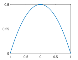
(a) Initial value $u_{0}(x)$

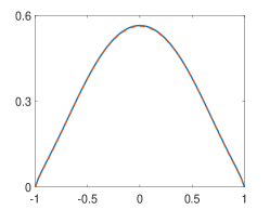
(b) An index-1 saddle point

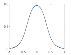
(c) An index-2 saddle point

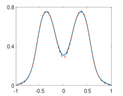
(d) An index-3 saddle point

Figure 1: Plots of $u_{0}(x)$ in (a) and the approximated saddle points by SD (blue solid) and GPSD (red dashed) for the cases (i)–(iii) in (b)–(d), respectively.

Table 5: Comparison of the number of force evaluation $N_{f}$ in SD and GPSD for computing the saddle points of the nonlocal phase field model (11)

	$N_{f}$ in SD	$N_{f}$ in GPSD
(i)	18225	960
(ii)	95125	3480
(iii)	117516	4200

Figure 2: Solution landscape of nonlocal phase-field model (11) constructed by (left) SD and (right) GPSD based downward search algorithm.

5 Concluding remarks

In this work we propose a model-free shrinking-dimer saddle dynamics and a corresponding sequential learning algorithm for finding any-index saddle points of complex models and constructing their solution landscapes. This data-driven approach avoids employing the exact form of the model and could significantly reduce the number of queries of the force that may be expensive or time-consuming, and the active learning mechanism along the latent trajectory increases the value of each sampling. More importantly, with the proposed algorithm, we can efficiently construct the model-free solution landscape, in which only the informative saddle points and minima are computed, so that one can avoid the sampling on the whole energy landscape of complex models.

There are several potential extensions of the current method. For instance, different covariance kernels in the Gaussian process or different learning methods such as the deep learning method could be applied to train the surrogate model. The proposed data-driven method could be further applied for constructing the solution landscapes of more complex problems, and how to utilize the structure of the solution landscape to further reduce the number of queries of the force is an interesting but challenging problem that will be investigated in the near future.

Acknowledgments We greatly appreciate Dr. Siwei Duo for providing the MATLAB code of computing the fractional Laplacian in DuoZha .

Declarations

Funding: This work was partially supported by the National Key R&D Program of China No. 2021YFF1200500 and the National Natural Science Foundation of China No. 12225102, 12050002, 12288101.
Conflict of interest: The authors have no conflict of interest.
Authors’ contributions: Lei Zhang: Conceptualization, Funding acquisition, Methodology, Supervision, Writing – review & editing. Pingwen Zhang: Funding acquisition, Supervision. Xiangcheng Zheng: Formal analysis, Funding acquisition, Investigation, Methodology, Visualization, Writing – original draft.

References

- (1) J. Foresman, M. Head-Gordon, J. Pople, M. Frisch, Toward a systematic molecular orbital theory for excited states. J. Phys. Chem. 96 (1992), 135–149.
- (2) J. Allison, T. Guo, Z. Han, Co-design of an active suspension using simultaneous dynamic optimization. ASME J. Mech. Des. 136 (2014), 081003.
- (3) D. Branduardi, F. Gervasio, M. Parrinello, From a to b in free energy space. J. Chem. Phys. 126 (2007), 054103.
- (4) C. Chen and Z. Xie, Search extension method for multiple solutions of a nonlinear problem. Comput. Math. Appl. 47 (2004), pp. 327–343.
- (5) A. Denzel and J. Kastner, Gaussian process regression for transition state search. J. Chem. Theory Comput. 14 (2018), 5777–5786.
- (6) A. Deshmukh and J. Allison, Design of dynamic systems using surrogate models of derivative functions. ASME. J. Mech. Des. 139 (2017), 101402.
- (7) S. Duo and H. Wang, A fractional phase-field model using an infinitesimal generator of stable Lévy process. J. Comput. Phys. 384 (2019), 253–269.
- (8) S. Duo and Y. Zhang, Computing the ground and first excited states of the fractional schrödinger equation in an infinite potential well. Commun. Comput. Phys. 18 (2015), 321–350.
- (9) W. E and X. Zhou, The gentlest ascent dynamics. Nonlinearity 24 (2011), 1831–1842.
- (10) M. D’Elia, Q. Du, C. Glusa, M. Gunzburger, X. Tian, Z. Zhou, Numerical methods for nonlocal and fractional models. Acta Numerica 29 (2020), 1–124.
- (11) N. Gould, C. Ortner and D. Packwood, A dimer-type saddle search algorithm with preconditioning and linesearch. Math. Comp. 85 (2016), 2939–2966.
- (12) S. Gu, H. Wang, X. Zhou, Active learning for transition state calculation. J. Sci. Comput. 93 (2022), 78.
- (13) Y. Han, J. Yin, P. Zhang, A. Majumdar, L. Zhang, Solution landscape of a reduced Landau–de Gennes model on a hexagon. Nonlinearity 34 (2021), 2048–2069.
- (14) Y. Han, J. Yin, Y. Hu, A. Majumdar, L. Zhang, Solution landscapes of the simplified Ericksen-Leslie model and its comparison with the reduced Landau-de Gennes model. Proc. Roy. Soc. A-Math. Phy., 477 (2021), 20210458.
- (15) D. Heidrich and W. Quapp, Saddle points of index 2 on potential energy surfaces and their role in theoretical reactivity investigations. Theor. Chim. Acta, 70 (1986), 89-98.
- (16) G. Henkelman and H. Jónsson, A dimer method for finding saddle points on high dimensional potential surfaces using only first derivatives. J. Chem. Phys. 111 (1999), 7010–7022.
- (17) O. Koistinen, F. Dagbjartsdóttir, V. Ásgeirsson, A. Vehtari, H. Jónsson, Nudged elastic band calculations accelerated with Gaussian process regression. J. Chem. Phys. 147 (2017), 152720.
- (18) Y. Li and J. Zhou, A minimax method for finding multiple critical points and its applications to semilinear PDEs, SIAM J. Sci. Comput. 23 (2001), 840–865.
- (19) A. Lischke, G. Pang, M. Gulian, F. Song, C. Glusa, X. Zheng, Z. Mao, W. Cai, M. Meerschaert, M. Ainsworth, G. Karniadakis, What is the fractional Laplacian? A comparative review with new results. J. Comput. Phys. 404 (2020), 109009.
- (20) H. Liu, J. Cai, Y. Ong, Remarks on multi-output Gaussian process regression. Knowledge-Based Syst. 144 (2018), 102–121.
- (21) X. Liu, Q. Zhu, H. Lu, Modeling multiresponse surfaces for airfoil design with multiple-output-Gaussian-process regression. J. Aircraft 51 (2014), 740–747.
- (22) Y. Luo, X. Zheng, X. Cheng, L. Zhang, Convergence Analysis of Discrete High-Index Saddle Dynamics. SIAM Journal on Numerical Analysis, 60 (2022), 2731–2750.
- (23) D. Mehta, Finding all the stationary points of a potential-energy landscape via numerical polynomial-homotopy-continuation method, Phys Rev E 84 (2011) 025702.
- (24) J. W. Milnor, Morse Theory, Princeton University Press, 1963.
- (25) Q. Nie, L. Qiao, Y. Qiu, L. Zhang, W. Zhao, Noise control and utility: from regulatory network to spatial patterning. Sci. China Math., 63 (2020), 425–440.
- (26) M. Powel, Algorithms for nonlinear constraints that use Lagrangian function. Math. Programming 14 (1978), 224–248.
- (27) M. Raissi, P. Perdikaris, G. Karniadakis, Machine learning of linear differential equations using Gaussian processes. J. Comput. Phys. 348 (2017), 683–693.
- (28) C. Rasmussen and C. Williams, Gaussian processes for machine learning. MIT Press, 2006.
- (29) C. Sheng, J. Shen, T. Tang, L. Wang, H. Yuan, Fast Fourier-like mapped Chebyshev spectral-Galerkin methods for PDEs with integral fractional Laplacian in unbounded domains. SIAM J. Numer. Anal. 58 (2020), 2435–2464.
- (30) B. Shi, Y. Han, L. Zhang, Nematic Liquid Crystals in a Rectangular Confinement: Solution Landscape, and Bifurcation. SIAM Journal on Applied Mathematics, 82 (2022), 1808–1828.
- (31) F. Song, C. Xu, G. Karniadakis, A fractional phase-field model for two-phase flows with tunable sharpness: algorithms and simulations. Comput. Methods Appl. Mech. Engrg. 305 (2016), 376–404.
- (32) B. Tang, Orthogonal array-based Latin hypercubes. J Amer. Stat. Assoc. 88 (1993), 1392–1397.
- (33) W. Wang, L. Zhang, P. Zhang, Modelling and computation of liquid crystals. Acta Numerica 30 (2021), 765–851.
- (34) J. Yin, K. Jiang, A.-C. Shi, P. Zhang, L. Zhang, Transition pathways connecting crystals and quasicrystals. Proc. Natl. Acad. Sci. U.S.A. 118 (2021), e2106230118.
- (35) J. Yin, Y. Wang, J. Chen, P. Zhang, L. Zhang, Construction of a pathway map on a complicated energy landscape. Phys. Rev. Lett. 124 (2020), 090601.
- (36) J. Yin, L. Zhang, P. Zhang, High-index optimization-based shrinking dimer method for finding high-index saddle points. SIAM J. Sci. Comput. 41 (2019), A3576–A3595.
- (37) J. Yin, B. Yu, L. Zhang, Searching the solution landscape by generalized high-index saddle dynamics. Sci. China Math. 64 (2021), 1801.
- (38) B. Yu, X. Zheng, P. Zhang, L. Zhang, Computing solution landscape of nonlinear space-fractional problems via fast approximation algorithm. J. Comput. Phys. 468 (2022), 111513.
- (39) J. Zhang, Q. Du, Shrinking dimer dynamics and its applications to saddle point search. SIAM J. Numer. Anal. 50 (2012), 1899–1921.
- (40) J. Zhang and Q. Du, Constrained shrinking dimer dynamics for saddle point search with constraints. J. Comput. Phys. 231 (2012), 4745–4758.
- (41) L. Zhang, L. Chen, Q. Du, Morphology of critical nuclei in solid-state phase transformations. Phys. Rev. Lett. 98 (2007), 265703.
- (42) L. Zhang, L. Chen, Q. Du, Simultaneous prediction of morphologies of a critical nucleus and an equilibrium precipitate in solids. Commun. Comput. Phys. 7 (2010), 674–682.
- (43) L. Zhang, Q. Du, Z. Zheng, Optimization-based shrinking dimer method for finding transition states. SIAM J. Sci. Comput. 38 (2016), A528–A544.
- (44) L. Zhang, W. Ren, A. Samanta, and Q. Du, Recent developments in computational modelling of nucleation in phase transformations. NPJ Comput. Materials 2 (2016), 16003.
- (45) L. Zhang, P. Zhang, X. Zheng, Error estimates of Euler discretization to high-index saddle dynamics. SIAM J. Numer. Anal. 60 (2022), 2925–2944.