Universal Method to Estimate Quantum Coherence

Abstract

Coherence is a defining property of quantum theory that accounts for quantum advantage in many quantum information tasks. Although many coherence quantifiers have been introduced in various contexts, the lack of efficient methods to estimate them restricts their applications. In this paper, we tackle this problem by proposing one universal method to provide measurable bounds for most current coherence quantifiers. Our method is motivated by the observation that the distance between the state of interest and its diagonal parts in reference basis, which lies at the heart of the coherence quantifications, can be readily estimated by disturbance effect and uncertainty of the reference measurement. Thus, our method of bounding coherence provides a feasible and broadly applicable avenue for detecting coherence, facilitating its further practical applications.

I I. Introduction

Coherence, captured by the superposition principle, is a defining property of quantum theory. It underscores almost all the quantum features, such as symmetry Marvian and Spekkens (2014), entanglement Streltsov et al. (2015); Chitambar and Hsieh (2016); Zhu et al. (2018), quantum correlation Hu et al. (2018a); Ma et al. (2016). Coherence also accounts for quantum advantages in various quantum information processing tasks, such as quantum metrology Giovannetti et al. (2011); Giorda and Allegra (2017); Kwon et al. (2019) and quantum cryptography Huttner et al. (1995); Ma et al. (2019). Within a strictly mathematical framework of resource theory, the significance of coherence as a resource has been fully appreciated in recent years. Many aspects of it, ranging from characterization Streltsov et al. (2017), distillation, and, catalytic Chitambar and Gour (2016a, b); Chitambar and Gour (2019); Åberg (2014), have been investigated, along with intense analysis of how coherence plays a role in fundamental physics (see  Hu et al. (2018b) for a review).

Quantifying coherence lies in the heart of coherence resource theory Oi and Åberg (2006); Girolami (2014); Streltsov et al. (2017); Winter and Yang (2016); Rastegin (2016); Yu (2017); Liu et al. (2017a). Till now, many methods have been proposed. The most initiative method is based on state distance, for example, quantifying coherence with the minimal distance between the state of interest and the closest coherence free state. The typical examples are the relative entropy of coherence and the $l_{1}-$norm of coherence Winter and Yang (2016). Coherence may also be quantified with the distance between the concerned state and its diagonal parts in the reference basis Liu et al. (2017b). One example is the coherence of trace-norm Cui et al. (2020); Biswas et al. (2017). Another method is via the convex roof measure. That is, provided a quantifier for the pure state, a general mixed state’s quantifier is constructed via a roof construction, which method leads to the formation of coherence Yuan et al. (2015) and infidelity coherence measureLiu et al. (2017a). There are also other quantifiers such as the robustness of coherence Napoli et al. (2016), and the Wigner-Yanase skew information of coherence Yu (2017).

While many theoretical works have been devoted to a systematical research of coherence Baumgratz et al. (2014); Yu et al. (2016); Hu et al. (2018b); Streltsov et al. (2017), it remains a difficult problem to efficiently estimate coherence in experiments, which limits the applications of the quantifications as common tools for quantum information processing. Clearly, one can perform state tomography and then calculates quantifiers with the derived quantum density matrix, or estimate coherence by employing normal witness technique Piani et al. (2016); Wang et al. (2017); Zheng et al. (2018) and with numerical optimizations Zhang et al. (2018). These methods suffer from the complexities of mathematics and experiment setup thus lacking efficiency. Another method is based on spectrum estimation Yu and Gühne (2019), which commonly needs a few test measurements to obtain a non-trivial estimation. These methods, unfortunately, are commonly restricted for estimating the convex roof quantifiers, such as the coherence of formation, convex roof of infidelity, and convex roof of the Wigner-Yanase skew information.

To improve the evaluation of coherence in experiments, we report one simple and feasible detection method, which provides both the upper and the lower bounds in terms of the reference measurement’s uncertainty and disturbance effect, respectively. We find that coherence quantifiers are closely related to the distance between the state of interest and its diagonal parts( written in the reference basis). The distance can be upper-bounded in terms of uncertainty according to recent uncertainty-disturbance relations (UDR) Sun et al. (2022a, b) and lower-bounded according to data processing inequality. These bounds are formulated with statistics from a universal experiment scheme. By the method, almost all the current coherence quantifiers of great interests are immediately bounded as long as one universal experiment setup output statistics. The quantifiers include the relative entropy of coherence measure, the coherence of formation, the $l_{1}-$norm of coherence, the $l_{2}-$ norm of coherence, the trace-norm of coherence, the convex roof of infidelity coherence, the Wigner-Yanase skew information of coherence and the convex roof construction, and the robustness of coherence. Thus the method exhibits merits of simplicity and broad applicability.

The rest of the paper is structured as follows. In section I, we briefly review state-distance based coherence quantifiers, then provide framework for upper-bounding and lower-bounding them. In section II, we provide measurable bounds for most current coherence quantifiers, including the distance-based quantifiers and some other quantifiers of general interests. In section III, we compare our method with the one based on spectrum estimation, showing that our method is experimentally less demanding and more efficient.

II II. The Framework of Detecting Coherence

II.1 A.The distance-based quantifications of coherence

Coherence is a quantity characterized with respect to one prefixed reference basis denoted by $\{|j\rangle\}$ with the revelent measurement being referred to as reference measurement. The free states are the ones of the form $\sigma=\sum_{j}p_{j}|j\rangle\langle j|$. Otherwise, a non-diagonal state contains coherence. Coherence is commonly quantified with state distance, for example, with the minimal distance between the state of interest and the closest incoherent one Chitambar and Gour (2019)

$$\mathcal{C}(\rho):=\min_{\sigma\in\mathcal{I}}\mathcal{D}(\rho,\sigma),$$ (1)

where $\mathcal{I}$ denotes the set of coherence free states, and $\mathcal{D}(\rho,\sigma)$ specifies state distance. Apply Eq.(1) to the state distances of relative entropy, $l_{1}-$norm,the Tsallis relative $\alpha-$ entropies, one can define quantifiers meeting all the criteria of the coherence resource theory Streltsov et al. (2017). They are referred to as coherence measures. If the chosen distance measures are trace-norm and fidelity Shao et al. (2015); Rana et al. (2016), Eq.(1) defines coherence monotones that meet a specific subset of the criteria of the coherence resource theory.

The computability of quantifier $\mathcal{C}(\rho)$ is generally hard except the state distance, for which, $\mathcal{C}(\rho)=\mathcal{D}(\rho,\rho_{d})$, where $\rho_{d}$ specifies the diagonal parts of $\rho$ in the reference basis. One may simply define an easily computable quantifier as the distance between $\rho$ and $\rho_{d}$ Liu et al. (2017b):

$$\tilde{\mathcal{C}}(\rho):=\mathcal{D}(\rho,\rho_{d}),$$ (2)

which can be understood as the disturbance caused by reference measurement in $\rho$ as $\rho_{d}$ is just the post-measurement state. For some distance measures, Eq.(2) defines a better monotone than the one defined by Eq.(1). One example is trace-norm Cui et al. (2020), for which, Eq.(2) defines a quantifier that can satisfy more criteria (than the defined by Eq.(1)) and also allows a physically well-motivated interpretation as the capability to exhibit interference visibility Biswas et al. (2017). $\tilde{\mathcal{C}}(\rho)$ does not involve a minimization process. Therefore,

$$\tilde{\mathcal{C}}(\rho)\geq\mathcal{C}(\rho).$$

One may also define coherence quantifier via a convex roof technique Yuan et al. (2015). That is, provided a quantifier for pure state, one can define a mixed state’s quantifier via a convex roof construction. For example, one may define the pure state coherence via Eq.(1), then the convex roof construction is

$$\mathcal{C}^{\prime}(\rho):=\textstyle\min_{\{f_{i},|\phi_{i}\rangle\}}\sum_{i}f_{i}\cdot\mathcal{C}(\phi_{i}),$$ (3)

where the minimization is taken over all the possible pure state decompositions of $\rho=\sum f_{i}|\phi_{i}\rangle\langle\phi_{i}|$. This definition has its advantage, e.g., when applied to infidelity, Eq.(3) can define a measure Liu et al. (2017a) for coherence while Eq.(1) defines only a monotone.

The above definitions have led to many quantifiers and also induce the bounds for the quantifiers defined in other ways. In the following, we first introduce a framework for bounding them.

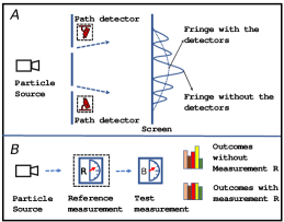
Figure 1: Two-slit experiment and coherence detection protocol. Particles with and without coherence leads to different statistics when subjected to a test measurement.

II.2 B. The framework of detecting coherence

Detecting the nonclassical properties, such as entanglement, coherence, and randomness, is to lower-bound them using the statistics coming from experiments. For coherence, it is instructive to recall its early illustration based on the two-slit experiment which is shown in Fig.1A, where the reference measurement is the path detectors that erases the coherence between paths, and the screen is an incompatible measurement that verifies the coherence in terms of the change of interference fringes due to the destroy of coherence. Here, we would like to exploit how this idea applies to many other coherence quantifiers. We consider a similar measurement setting as shown in Fig1.B. It consists of one reference measurement $\mathcal{R}$ and one following test measurement $\mathcal{B}$. The reference measurement updates an input state $\rho$ into an incoherent state, $i.e.$, its diagonal parts $\rho_{d}$. It then is subject to a following measurement $\mathcal{B}=\{|b_{j}\rangle\langle b_{j}|\}$, giving rise to a distribution $\mathbf{q^{\prime}}=\{q^{\prime}_{j}=\operatorname{tr}(\rho_{d}\cdot|b_{j}\rangle\langle b_{j}|)\}$. This is a typical sequential measurement scheme that can be readily realised with off-the-shelf instruments Pryde et al. (2005); Kaneda et al. (2014); Weston et al. (2013); Marques et al. (2014). If without the measurement $\mathcal{R}$, directly performing $\mathcal{B}$ on $\rho$ yields a distribution $\mathbf{q}=\{q_{j}=\operatorname{tr}(\rho\cdot|b_{j}\rangle\langle b_{j}|)\}$. Distance between $\mathbf{q}$ and $\mathbf{q}^{\prime}$ can be understood as the disturbance introduced by the reference measurement in $\mathcal{B}$. One may choose $\mathcal{B}$ as the one maximally incompatible with the reference measurement, $i.e.$, $\forall i,j$, $|\langle i|b_{j}\rangle|^{2}=\frac{1}{d}$ with $d$ specifying dimension of the revelent Hilbert’s space. This setting commonly can ensure a significant distance between $\mathbf{q}$ and $\mathbf{q}^{\prime}$, which is in favour of coherence estimation. We also note that $\mathbf{q}^{\prime}$ actually does not require performing a real test measurement after the reference measurement. As $\rho_{d}$ is determined by the reference measurement’s distribution as $\rho_{d}=\sum_{i}p_{i}|i\rangle\langle i|$ and $\mathbf{p}=\{p_{i}=\operatorname{tr}(\rho\cdot|i\rangle\langle i|)\}$, one can directly calculate $\mathbf{q}^{\prime}$ via Born’s rule. For example, the probability when $\mathcal{B}:=\{|b_{j}\rangle\langle b_{j}|\}$ is $q^{\prime}_{i}=\operatorname{tr}(\rho_{d}\cdot|b_{i}\rangle\langle b_{j}|)=\sum_{i}c_{ij}p_{i}$ is given by $\mathbf{p}$, where $c_{ij}=|\langle i|b_{j}\rangle|^{2}$. In this way, only two independent measurements, namely, $\mathcal{R}$ and $\mathcal{B}$, are sufficient for giving the statistics $\mathbf{p}$, $\mathbf{q}$, and $\mathbf{q}^{\prime}$. In the following, the estimation of coherence quantifiers only involves these distributions.

Lower-bounding coherence First, the coherence quantifiers of the form Eq.(2) can be estimated according to data processing inequality, which states that distance between states, say $\rho$ and $\rho_{d}$, are no less than the corresponding classical distance between statistics coming from another measurement, say, $\mathcal{B}$, performed on them:

$$\mathcal{D}(\rho,\rho_{d})\geq\operatorname{D}[\mathbf{q},\mathbf{q}^{\prime}].$$

Immediately, we obtain a lower bound for the coherence measure

$$\tilde{\mathcal{C}}(\rho)\geq\operatorname{D}[\mathbf{q},\mathbf{q}^{\prime}].$$ (4)

We highlight a useful property of the classical distance, namely, the convexity of classical distance $\operatorname{D}$,

$$\textstyle\sum_{i}f_{i}\cdot\operatorname{D}[\mathbf{q}_{i},\mathbf{q}^{\prime}_{i}]\geq\operatorname{D}[\sum_{i}f_{i}\cdot\mathbf{q}_{i},\sum_{i}f_{i}\cdot\mathbf{q}_{i}^{\prime}],$$

which will be used for bounding $\mathcal{C}^{\prime}(\rho)$.

Second, we consider the convex roof-based coherence quantifier. We note that for pure state a coherence quantifier $\mathcal{C}^{\prime}(\phi)$ is always a function of distribution $\mathbf{p}_{\phi}$. This is because the diagonal elements of a pure state are sufficient to determine coherence quantifier as they determine a pure state up to some relative phases. These phases are inessential in quantifying coherence as they can be modified freely with reversible incoherent operation of phase shifting. Noting that the maximum coherent state $|\phi\rangle=\frac{1}{d}\sum_{i}|i\rangle$ and the zero-coherence pure state $|i\rangle\langle i|$ exhibit the maximum and the minimal, respectively, uncertainty of reference measurement in the give basis. It is therefore reasonable to assume that the coherence quantifier $\mathcal{C}^{\prime}(\phi)$ for pure state is positively related with uncertainty $\delta_{\mathcal{D}}(\mathbf{p})$ (the subscript means that uncertainty can be related to state distance $\mathcal{D}$) and may be lower-bounded with uncertainty or a function of it (whose definition is left in the next section). We find that, if a pure state coherence $\mathcal{C}^{\prime}(\phi)$ allows a lower bound in terms of a convex and monotonically increasing function of $\delta_{\mathcal{D}}(\mathbf{p}_{\phi})$ specified by $g(\delta_{\mathcal{D}})$, the constructed convex roof-based coherence quantifier $\mathcal{C}^{\prime}(\rho)$ can be lower-bounded as

$$\mathcal{C}^{\prime}(\rho)\geq g(\operatorname{D}(\mathbf{q},\mathbf{q}^{\prime})).$$ (5)

It needs to be stressed that $\mathcal{C}^{\prime}(\rho)\geq g(\delta_{\mathcal{D}}(\mathbf{p}))$ generally does not hold for a mixed state $\rho$ due to the concavity of $\delta_{\mathcal{D}}$, namely, $\mathcal{C}^{\prime}(\rho)\geq\sum_{i}f_{i}\cdot g(\delta_{\mathcal{D}}(\mathbf{p}_{i}))\geq g(\sum_{i}f_{i}\cdot\delta_{\mathcal{D}}(\mathbf{p}_{i}))$ while $g(\sum_{i}f_{i}\cdot\delta_{\mathcal{D}}(\mathbf{p}_{i}))\leq g(\delta_{\mathcal{D}}(\mathbf{p}))$, where $\sum_{i}\mathbf{p}_{i}=\mathbf{p}$ and $\sum_{i}f_{i}\cdot\mathbf{p}_{i}=\mathbf{p}$. The key idea behind Eq.(5) is to relax a concave uncertainty measure $\delta_{\mathcal{D}}$ into a convex disturbance measure $\operatorname{D}(\mathbf{q},\mathbf{q}^{\prime})$ using UDRs Sun et al. (2022b) stating that one measurement’s uncertainty in terms of, say $\delta_{\mathcal{D}}(\mathbf{p})$, is no less than its disturbance effect in the measured state $\rho$ and in the subsequent test measurement $\mathcal{B}$:

$$\delta_{\mathcal{D}}(\mathbf{p})\geq\mathcal{D}(\rho,\rho_{d})\geq\operatorname{D}(\mathbf{q},\mathbf{q}^{\prime}).$$

Then, we have $g(\sum_{i}f_{i}\cdot\operatorname{D}(\mathbf{q}_{i},\mathbf{q}^{\prime}_{i}))\geq g(\operatorname{D}(\mathbf{q},\mathbf{q}^{\prime}))$ with $\sum_{i}f_{i}\cdot\mathbf{q}_{i}=\mathbf{q}$ and $\sum_{i}f_{i}\cdot\mathbf{q}^{\prime}_{i}=\mathbf{q}^{\prime}$, leading to a lower-bound for coherence quantifiers. We left the proof of Eq.(5) in SM. It can be seen that the function of $g(\cdot)$ provides a way of finding the lower-bound of coherence measure in terms of disturbance $\operatorname{D}(\mathbf{q},\mathbf{q}^{\prime})$. In the next section, we shall show that $g(\cdot)$ can always be found for the existing convex roof-based coherence quantifiers.

Estimation of upper-bounds In general, upper bounds for quantum properties are not as useful as the lower bounds since they may be way larger than the actual value and thus are commonly ignored in theory and experiment. Here, we can obtain the estimation of the upper bound with the outcome distribution of the reference measurement for free, i.e., without introducing extra experiment settings, and most importantly the resulting upper bound may assist the estimation of coherence in our framework.

It follows from the UDRs that the upper bounds of the quantifiers of the form Eq.(1) or Eq.(2) are given as

$$\delta(\mathbf{p})\geq\tilde{\mathcal{C}}(\rho)\geq\mathcal{C}(\rho).$$ (6)

The upper bound of $\mathcal{C}^{\prime}(\rho)$ is given as

$$\delta(\mathbf{p})\geq\sum_{i}f_{i}\cdot\delta(\mathbf{p}_{i})\geq\sum_{i}f_{i}\cdot\mathcal{C}(\phi_{i})=\mathcal{C}^{\prime}(\rho),$$ (7)

Thus, one reference measurement is sufficient for upper-bounding the three kinds of coherence quantifiers.

Till now, with the distributions of $\mathbf{p}$, $\mathbf{q}$, and $\mathbf{q}^{\prime}$, both the upper and the lower bounds are obtained. A possible large gap between them roughly indicates that: (i) the state of interest contains little coherence, and (ii) the setting of $\mathcal{B}$ is not well-chosen. Then the lower bound may be optimized by choosing other settings of $\mathcal{B}$ or one may almost confirm that the state of interest contains little coherence. In this way the upper bound assists the estimation of lower bound.

III III. Detecting Coherence in Various contexts

In the following, we use the above framework to estimate coherence quantifiers having general interests.

III.1 A. The relative entropy of coherence measure and the coherence of formation

First, we consider the relative entropy of coherence Baumgratz et al. (2014) and the coherence of formation Åberg (2006); Oi and Åberg (2006); Yuan et al. (2015), which are defined by applying Eq.(1) and Eq.(3) to the relative entropy

$$S(\rho\|\sigma):=\operatorname{Tr}(\rho\log\rho-\rho\log\sigma).$$

Relative entropy of coherence is a legitimate measure. It has operational meaning as asymptotic coherence distillation rate Winter and Yang (2016) and also quantifies the quantum randomness under the quantum adversaries (with independent measurements) Yuan et al. (2015); Liu et al. (2018); Yuan et al. (2019). The quantifier is defined as

$$\mathcal{C}_{re}(\rho):=\min_{\sigma\in\mathcal{I}}S(\rho\|\sigma)=S(\rho\|\rho_{d}).$$

The coherence of formation has an interpretation of the asymptotic coherence dilution rate Winter and Yang (2016). It also quantifies the quantum randomness under the classical adversaries (with independent measurements) Yuan et al. (2015); Liu et al. (2018); Yuan et al. (2019). The quantifier reads

$$\mathcal{C}^{\prime}_{re}(\rho):=\min_{\{f_{i},\phi_{i}\}}\sum_{i}f_{i}\cdot S(\phi_{i}\|\phi_{i,d}).$$

The UDR corresponding to the relative entropy is given as

$$\operatorname{H}(\mathbf{p})\geq S(\rho\|\rho_{d})\geq\operatorname{H}(\mathbf{q}\|\mathbf{q}^{\prime}),$$

where the Shannon entropy $\operatorname{H}(\mathbf{p}):=-\sum_{i}p_{i}\log p_{i}$ defines measurement uncertainty $\delta_{re}(\mathbf{p})$ and the relative entropy $S(\rho\|\rho_{d})$ defines disturbance in quantum state and the classical relative entropy $\operatorname{H}(\mathbf{q}\|\mathbf{q}^{\prime}):=\sum_{i}q_{i}\log q_{i}-\sum_{i}q_{i}\log q^{\prime}_{i}$ defines the disturbance in measurement $\mathcal{B}$ denoted with $\rm D_{re}(\mathbf{q},\mathbf{q}^{\prime})$. Based on the general arguments just provided, we immediately have Sun et al. (2022b)

$$\operatorname{H}(\mathbf{p})\geq\mathcal{C}_{re}(\rho),\quad\mathcal{C}^{\prime}_{re}(\rho)\geq\operatorname{H}(\mathbf{q}\|\mathbf{q}^{\prime}).$$ (8)

For $\mathcal{C}_{re}(\rho)$, the bounds are obvious. For $\mathcal{C}^{\prime}_{re}(\rho)$, we have $\mathcal{C}^{\prime}_{re}(|\phi\rangle)=\operatorname{H}(\mathbf{p}_{\phi})$, which leads to a definition of convex and monotonically increasing $g$ function as $g(x)=x$. Then a lower bound for $\mathcal{C}^{\prime}_{re}(\rho)$, namely, $\operatorname{H}(\mathbf{q}\|\mathbf{q}^{\prime})$, follows from Eq.(5) and uncertainty disturbance relation Sun et al. (2022b).

III.2 B. The $l_{1}-$norm, the $l_{2}-$ norm, and the trace-norm of coherence

The $l_{1}-$norm of coherence. The $l_{1}-$norm of coherence quantifies the maximum entanglement that can be created from coherence under incoherent operations acting on the system and an incoherent ancilla Zhu et al. (2018). It has been used to investigate the speed-up of quantum computation Hillery (2016); Shi et al. (2017), wave-particle duality Hu et al. (2018b); Bera et al. (2015); Cheng and Hall (2015), and uncertainty principle Yuan et al. (2017). The quantifier is defined via Eq.(1) as Baumgratz et al. (2014)

$$\mathcal{C}_{l_{1}}(\rho)=\min_{\sigma\in\mathcal{I}}\mathcal{D}_{l_{1}}(\rho,\sigma)=\mathcal{D}_{l_{1}}(\rho,\rho_{d}).$$

where the $l_{1}-$norm

$$\mathcal{D}_{l_{1}}(\rho,\sigma^{\prime})=\textstyle\sum_{i,j}|\rho_{ij}-\sigma^{\prime}_{ij}|$$

with $\rho_{ij}$ and $\sigma^{\prime}_{ij}$ specifying matrixes’ elements.

The UDR corresponding to the $l_{1}-$norm distance is

$$\|\mathbf{p}\|_{\frac{1}{2}}-1\geq\mathcal{D}_{l_{1}}(\rho,\rho_{d}),$$

where $\|\mathbf{p}\|_{x}=(\sum_{i}p^{x}_{i})^{\frac{1}{x}}$. The inequality is because that $\sum_{i\neq j}|\rho_{ij}|\leq\sum_{i\neq j}\sqrt{p_{i}p_{j}}=\|\mathbf{p}\|_{\frac{1}{2}}-1$. Based on Eq.(6) and the UDR, the $\mathcal{C}_{l_{1}}(\rho)$ is estimated via

$$\|\mathbf{p}\|_{\frac{1}{2}}-1\geq\mathcal{C}_{l_{1}}(\rho)\geq 2|\mathbf{q}-\mathbf{q}^{\prime}|,$$ (9)

where $|\mathbf{q}-\mathbf{q}^{\prime}|:=\frac{1}{2}\sum_{i}|q_{i}-q^{\prime}_{i}|$ is the Kolmogorov distance. The lower bound side is due to $\sum_{i\neq j}|\rho_{ij}|=\sum_{i>j}$$\operatorname{tr}|\varrho_{ij}|\geq\operatorname{tr}|\rho-\rho_{d}|\geq 2|\mathbf{q}-\mathbf{q}^{\prime}|$, where $\operatorname{tr}|A|=\operatorname{tr}\sqrt{AA^{\dagger}}$ and $\varrho_{ij}:=|j\rangle\langle j|\rho|i\rangle\langle i|+|i\rangle\langle i|\rho|j\rangle\langle j|$ and $\sum_{i\neq j}\operatorname{tr}|\varrho_{ij}|\geq\operatorname{tr}|\rho-\rho_{d}|$ is due to the convexity.

The $l_{2}-$norm of coherence. The $l_{2}-$norm of coherence Chitambar and Gour (2016b); Streltsov et al. (2017) has an operational interpretation as state uncertainty Sun and Luo (2021) and is also employed to study non-classical correlations Sun et al. (2017). The quantifier reads

$$\mathcal{C}_{l_{2}}(\rho):=\min_{\sigma\in\mathcal{I}}\mathcal{D}_{l_{2}}(\rho,\sigma)=\mathcal{D}_{l_{2}}(\rho,\rho_{d}),$$

where the $l_{2}-$norm or the (squared) Hilbert-Schmidt distance $\mathcal{D}_{l_{2}}(\rho,\sigma):=\operatorname{tr}(\rho-\sigma)^{2}.$

The UDR corresponding to $l_{2}-$norm is

$$1-\|\mathbf{p}\|^{2}_{2}\geq\mathcal{D}_{l_{2}}(\rho,\rho_{d}),$$

which is due to $\operatorname{tr}(\rho-\rho_{d})^{2}$$=\operatorname{tr}(\rho^{2}-\rho\cdot\rho_{d})\leq 1-\|\mathbf{p}\|^{2}_{2}$. Based on Eq.(6) and Eq.(4), $\mathcal{C}_{l_{2}}(\rho)$ is bounded as

$$1-\|\mathbf{p}\|^{2}_{2}\geq\mathcal{C}_{l_{2}}(\rho)\geq\|\mathbf{q}-\mathbf{q}^{\prime}\|^{2}_{2},$$ (10)

where the lower bound is due to data processing inequality with measurement $\mathcal{B}$ being required to be projective Ozawa (2000).

Trace-norm of coherence. The trace-norm of coherence has an interpretation of interference visibility and reads Cui et al. (2020)

$$\tilde{\mathcal{C}}_{tr}(\rho)=\rm\mathcal{D}_{tr}(\rho,\rho_{d})$$

where the distance of trace-norm $\mathcal{D}_{tr}(\rho,\sigma)=\textstyle\rm\frac{1}{2}tr|\rho-\sigma|.$ According to UDR corresponding to this distance Sun et al. (2022b)

$$\sqrt{1-\|\mathbf{p}\|^{2}_{2}}\geq\rm\mathcal{D}_{tr}(\rho,\rho_{d}),$$

we have

$$\sqrt{1-\|\mathbf{p}\|^{2}_{2}}\geq\tilde{\mathcal{C}}_{tr}(\rho)\geq|\mathbf{q}-\mathbf{q}^{\prime}|.$$ (11)

Again, the lower bound is due to data processing inequality.

III.3 C. Convex roof coherence of infidelity

Now, we consider the convex roof coherence of infidelity Liu et al. (2017a)

$$\mathcal{C}^{\prime}_{if}(\rho):=\textstyle\min_{\{f_{i},|\phi_{i}\rangle\}}\sum_{i}f_{i}\cdot\mathcal{C}_{if}(\phi_{i}),$$

where the pure state coherence is quantified as

$$\mathcal{C}_{if}(\phi)=\min_{\sigma\in\mathcal{I}}\mathcal{D}_{if}(\phi,\sigma)$$

with the infidelity $\mathcal{D}_{if}(\rho,\sigma):=\sqrt{1-\rm F(\rho,\sigma)}$ and $\operatorname{F}(\rho,\sigma)=[\rm Tr(\sqrt{\sqrt{\rho}\sigma\sqrt{\rho}})]^{2}$. The UDR corresponding to infidelity is Sun et al. (2022b).

$$\sqrt{1-\|\mathbf{p}\|_{2}^{2}}\geq\mathcal{D}_{if}(\rho,\rho_{d}).$$

By Eq.(7), the coherence measure acquires an upper bound as $\sqrt{1-\|\mathbf{p}\|_{2}^{2}}$.

To lower-bound the measure using Eq.(5), we note that $\mathcal{C}_{if}(\phi)\geq\frac{\sqrt{2}}{2}\sqrt{1-\|\mathbf{p}\|^{2}_{2}}:=\frac{\sqrt{2}}{2}\delta_{if}(\mathbf{p})$ (See SM), which leads to a definition of $g$ function as $g(x)=\frac{\sqrt{2}}{2}x$. By Eq(5), we have $\textstyle\mathcal{C}^{\prime}_{if}(\rho)\geq\frac{\sqrt{2}}{2}\operatorname{D}_{if}(\mathbf{q},\mathbf{q}^{\prime})$, where $\operatorname{D}_{if}(\mathbf{q},\mathbf{q}^{\prime}):=\textstyle\sqrt{1-(\sum_{i}\sqrt{q_{i}q^{\prime}_{i}})^{2}}.$ Thus, we finally have

$$\sqrt{1-\|\mathbf{p}\|_{2}^{2}}\geq\mathcal{C}^{\prime}_{if}(\rho)\geq\textstyle\frac{\sqrt{2}}{2}\operatorname{D}_{if}(\mathbf{q},\mathbf{q}^{\prime}).$$ (12)

Table 1: Measurable lower bounds for coherence quantifiers.

Quantifier	$\mathcal{C}_{re}$	$\mathcal{C}_{l_{1}}$	$\mathcal{C}_{l_{2}}$	$\tilde{\mathcal{C}}_{tr}$	$\mathcal{C}^{\prime}_{if}$	$C_{s}$	$C^{\prime}_{s}$	$C_{rob}$
Upper Bound	$\operatorname{H}(\mathbf{p})\quad$	$\|\mathbf{p}\|_{\frac{1}{2}}-1\quad$	$1-\|\mathbf{p}\|^{2}_{2}\quad$	$\sqrt{1-\|\mathbf{p}\|^{2}_{2}}\quad$	$\sqrt{1-\|\mathbf{p}\|^{2}_{2}}\quad$	$1-\|\mathbf{p}\|^{2}_{2}\quad$	$1-\|\mathbf{p}\|^{2}_{2}$	$\|\mathbf{p}\|_{\frac{1}{2}}-1$
Lower Bound	$\operatorname{H}(\mathbf{q}\|\mathbf{q}^{\prime})\quad$	$2|\mathbf{q}-\mathbf{q}^{\prime}|\quad$	$\|\mathbf{q}-\mathbf{q}^{\prime}\|^{2}_{2}\quad$	$|\mathbf{q}-\mathbf{q}^{\prime}|\quad$	$\frac{\sqrt{2}}{2}\operatorname{D}_{if}(\mathbf{q},\mathbf{q}^{\prime})\quad$	$\frac{1}{2}\|\mathbf{q}-\mathbf{q}^{\prime}\|^{2}_{2}\quad$	$\operatorname{D}^{2}_{if}(\mathbf{q},\mathbf{q}^{\prime})\quad$	$\frac{\|\mathbf{q}-\mathbf{q}^{\prime}\|^{2}_{2}}{\|\mathbf{p}\|_{\infty}}$

Till now, we have estimated many distance-based coherence quantifiers. In the following, we shall use the method to estimate the quantifiers going beyond the above definitions. The following quantifiers shall be specified by $C$ instead of $\mathcal{C}$ for the sake of specification.

III.4 D. The coherence of Wigner-Yanase skew information and the convex roof construction

Coherence can also be quantified based on quantum Fisher information, which is a basic concept in the field of quantum metrology that places the fundamental limit on the information accessible by performing measurement on quantum state. Two remarkable quantifiers are the Wigner-Yanase skew information of coherence and the convex roof construction based on it.

The Wigner-Yanase skew information of coherence. The Skew information coherence is a legitimate coherence measure and defined as Yu (2017)

$$C_{s}(\rho)=\textstyle\sum^{d}_{1=j}\operatorname{I}(\rho,|j\rangle\langle j|),$$

where $\operatorname{I}(\rho,|j\rangle\langle j|)\equiv-\frac{1}{2}\operatorname{Tr}([\rho,|j\rangle\langle j|])^{2}$ represents the Wigner-Yanase skew information subject to the projector $|j\rangle\langle j|$. This measure has ever been estimated with a spectrum estimation method employing the standard overlap measurement technique Yu (2017), where one needs to perform $2d-2$ measurements to estimate the coherence of a $d-$dimensional system. In the following, our method can reduce the number to three.

First, we can reexpress the measure as $\textstyle C_{s}(\rho)=1-\sum_{j}\langle j|\sqrt{\rho}|j\rangle^{2}$ Yu (2017), then an upper bound readily follows as

$$\textstyle C_{s}(\rho) = 1-\sum_{j}\langle j|\sqrt{\rho}|j\rangle^{2}\leq 1-\textstyle\sum_{j}\langle j|\rho|j\rangle^{2}$$

$$= 1-\|\mathbf{p}\|_{2}^{2}.$$

In order to derive a lower-bound, we use an inequality $C_{s}(\rho)\geq\frac{1}{2}\mathcal{C}_{l_{2}}(\rho)$ Yu (2017) whose bound has already been bounded in Eq.(10). Then, we have

$$1-\|\mathbf{p}\|_{2}^{2}\geq C_{s}(\rho)\geq\frac{1}{2}\|\mathbf{q}-\mathbf{q}^{\prime}\|^{2}_{2}.$$ (13)

The Convex Roof Construction. With $C_{s}(\phi)$ quantifying coherence of a pure state $|\phi\rangle$, the Wigner-Yanase skew information can lead to a convex roof construction of coherence as Li et al. (2021)

$$C^{\prime}_{s}(\rho)=\textstyle\min_{\{f_{i},\phi_{i}\}}\sum_{i}f_{i}\cdot C_{s}(\phi_{i}).$$

This quantifier can be equivalently defined via the quantum Fisher information (up to an inessential factor) with respective to reference measurement Yu (2013); Li et al. (2021):

$$C^{\prime}_{s}(\rho)=\frac{1}{4}\sum_{j}\operatorname{F}(\rho,|j\rangle\langle j|),$$

where $\operatorname{F}(\rho,|j\rangle\langle j|):=\sum_{k,l}2\frac{(\lambda_{k}-\lambda_{l})^{2}}{\lambda_{k}+\lambda_{l}}|c_{kl}|^{2}$ specifies quantum information of $\rho$ subject to the measurement projector $|j\rangle\langle j|$ and $c_{kl}=\langle\phi_{k}|j\rangle\langle j|\phi_{l}\rangle$ with $|\phi_{n}\rangle$ being the $n$th eigenvector of $\rho$ and $\lambda_{n}$ being the weight.

Given that $C_{s}(\phi)=1-\|\mathbf{p}(\phi)\|^{2}_{2}=\delta^{2}_{if}(\mathbf{p})$, we can define $g(\delta_{if})=\delta_{if}^{2}$. By Eq.(5), the lower bound of $C^{\prime}_{s}(\rho)$ follows as

$$C_{s}(\rho)\geq\operatorname{D}^{2}_{if}(\mathbf{q},\mathbf{q^{\prime}}).$$

Due to the convexity of $1-\|\mathbf{a}\|^{2}_{2}$ with respect to distribution $\mathbf{a}$, an upper bound is immediately obtained as

$$1-\|\mathbf{p}\|^{2}_{2}\geq C^{\prime}_{s}(\rho).$$

Thus, the quantifier is bounded as

$$1-\|\mathbf{p}\|^{2}_{2}\geq C^{\prime}_{s}(\rho)\geq\operatorname{D}^{2}_{if}(\mathbf{q},\mathbf{q^{\prime}})$$ (14)

III.5 F. The robustness of coherence

One important coherence monotone is the robustness of coherence Napoli et al. (2016), which quantifies the advantage enabled by a quantum state in a phase discrimination task. For a given state $\rho$, it is defined as the minimal mixing required to make the state incoherent

$$C_{Ro}(\rho)=\min_{\tau}\left\{s\geq 0\bigg{|}\frac{\rho+s\tau}{1+s}:=\sigma\in\mathcal{I}\right\}$$

where $\tau$ is a general quantum state. With the inequality Napoli et al. (2016)

$$C_{Ro}(\rho)\geq\frac{\mathcal{D}_{l_{2}}(\rho,\rho_{d})}{\|\rho_{d}\|_{\infty}}.$$

where note that $\|\rho_{d}\|_{\infty}=\|\mathbf{p}\|_{\infty}$ is just the maximum element in $\mathbf{p}$. It follows Eq.(10) that

$$C_{Ro}(\rho)\geq\frac{\|\mathbf{q}-\mathbf{q}^{\prime}\|^{2}_{2}}{\|\mathbf{p}\|_{\infty}}.$$

With the inequality $C_{Ro}(\rho)\leq\mathcal{C}_{l_{1}}(\rho)$ and Eq.(9), we have

$$\|\mathbf{p}\|_{\frac{1}{2}}-1\geq C_{Ro}(\rho)\geq\frac{\|\mathbf{q}-\mathbf{q}^{\prime}\|^{2}_{2}}{\|\mathbf{p}\|_{\infty}}.$$ (15)

The robustness of coherence has ever been detected based on the witness method Piani et al. (2016); Wang et al. (2017); Zheng et al. (2018), where the mathematics of constructing witness and experiment setup are generally complex.

Finally we summarize the obtained measurable lower bounds in Table.I. These bounds are all formulated in terms of the statistics $\mathbf{p}$, $\mathbf{q}$, and $\mathbf{q}^{\prime}$. As the essential quantity, the disturbance $\operatorname{D}$ can readily be measured by performing a sequential measurements scheme, which has been well-developed in the study of error-disturbance relations Pryde et al. (2005); Kaneda et al. (2014); Weston et al. (2013); Marques et al. (2014). In our approach, as the lower-bounds are smooth functions of experimental statistics, the statistics errors due to imperfection of implementation of measurement or state preparation are one order smaller comparing with the lower-bounds. These aspects make our protocol quite feasible.

It is also of practical interests to consider the tightness of these bounds. We find that the bounds of coherence measures $\mathcal{C}_{l_{2}}$ and $\tilde{\mathcal{C}}_{tr}$ can be saturated for any input state when the test measurement $\mathcal{B}$ is taken as the eigenvectors of $\rho-\rho_{d}$, and the bounds for the convex-roof based measure $C^{\prime}_{s}$ can be saturated if the concerned state is pure, and the bound of $\mathcal{C}_{l_{1}}$ is tight in qubit case (when $\mathcal{B}$ is taken as the eigenvectors of $\rho-\rho_{d}$). The bounds for other quantifiers either cannot not be non-trivially saturated or only be saturated for some specific states.

IV IV. Efficiency Argument

The previous coherence estimation protocols commonly apply to only a few coherence quantifiers. The collective measurement protocol Yuan et al. (2020) applies to the relative entropy of coherence and the $l_{2}-$norm of coherence. The witness method Piani et al. (2016); Wang et al. (2017); Zheng et al. (2018); Ma et al. (2021) applies to the robustness of coherence, the $l_{1}-$norm, and the $l_{2}-$norm of coherence. One quite simple and efficient method is based on spectrum estimation via majorization theory Yu and Gühne (2019), which can be used to estimate the $l_{1}-$norm, $l_{2}-$norm of coherence, the robustness of coherence, and the relative entropy of coherence. This method employs a similar measurement scheme to ours. In the following, we compare our approach with it.

IV.1 A. Comparison with the method based on spectrum estimation

The spectrum estimation method is based on the theory of majorization Yu and Gühne (2019). A probability $\mathbf{a}$ is said to majorize a probability distribution $\mathbf{b}$, specified as $\mathbf{a}\succeq\mathbf{b}$, if their elements satisfy $\sum^{k}_{i=1}a^{\downarrow}_{i}\geq\sum^{k}_{i=1}b^{\downarrow}_{i}$ $\forall k$, where the superscript means that the elements are arranged in a descending ordered, namely, $\mathbf{a}^{\downarrow}=(a^{\downarrow}_{1},a^{\downarrow}_{2},\cdots a^{\downarrow}_{d})$, $\mathbf{b}^{\downarrow}=(b^{\downarrow}_{1},b^{\downarrow}_{2},\cdots b^{\downarrow}_{d})$ with $a_{i}\geq a_{i+1}$ and $b_{i}\geq b_{i+1}$. Clearly, the spectrum of $\rho$, specified as $\boldsymbol{\lambda}=(\lambda_{1},\lambda_{2}\cdots\lambda_{d})$, majorizes distribution from any projection measurement, say $\mathcal{B}$, performed on $\rho$, $i.e.$, $\boldsymbol{\lambda}\succeq\mathbf{q}$. By the Shur convexity theorem, $\operatorname{H}(\mathbf{a})\geq\operatorname{H}(\mathbf{b})$ if $\mathbf{b}\succeq\mathbf{a}$. Thus, $\mathcal{C}_{r}(\rho)=\operatorname{H}(\mathbf{p})-\operatorname{H}(\boldsymbol{\lambda})\geq\operatorname{H}(\mathbf{p})-\operatorname{H}(\mathbf{q})$ with $\mathbf{p}$ and $\mathbf{q}$ being distributions from the reference measurement and $\mathcal{B}$, which provides a nontrivial lower bound if $\mathbf{q}\succ\mathbf{p}$. Generally, as state of interest is unknown one needs to try a few settings of $\mathcal{B}$ to ensure $\mathbf{q}\succ\mathbf{p}$. In this paper, we deal with the disturbance effect, namely, $\operatorname{D}(\mathbf{q},\mathbf{q}^{\prime})$, which is zero iff $\rho-\rho_{d}$ is perpendicular with all the elements of $\mathcal{B}$ simultaneously. The settings resulting in such a failure lie in a space of measure zero. Therefore, our method almost always works even the $\mathcal{B}$ is chosen arbitrarily. As a simple illustration, assume that $\rho$ is given as $|\phi\rangle=\sin\frac{\pi}{8}|0\rangle+\cos\frac{\pi}{8}|1\rangle$ and the reference basis is $\{|0\rangle,|1\rangle\}$, immediately, $\mathbf{p}=\{\sin^{2}\frac{\pi}{8},\cos^{2}\frac{\pi}{8}\}$. By the spectrum estimation method, a nontrivial estimation, namely, $\operatorname{H}(\mathbf{q})-\operatorname{H}(\mathbf{p})>0$ requires that $|\langle\phi|\mathcal{B}|\phi\rangle|>\cos^{2}\frac{\pi}{8}-\sin^{2}\frac{\pi}{8}=\frac{\sqrt{2}}{2}$. With our method, $\operatorname{D}(\mathbf{q},\mathbf{q}^{\prime})\neq 0$ requires that $\mathcal{B}\neq\sigma_{z},\sigma_{y}$, which is much weaker than the above requirement.

IV.2 B Numerical results for the qubit case

The lower bounds provided in Table.I work very well. As the second illustration of efficiency, we consider the qubit case. For the sake of computability, we let $\rho$ be a pure state. How well a quantifier is estimated can be naturally quantified with the ratio of the estimate to the exact value. For each quantifier, we calculate the average of the ratio over the randomly chosen measurement $\mathcal{B}$ and randomly chosen pure state (See SM for details) with two different methods, $i.e.$, our method and the one based on spectrum estimation. The averages are listed in the following table, where the one based on our method is specified by $Q^{C}_{D}$ and by $Q^{C}_{S}$ the other method.

Table 2: Efficiencies in estimating coherence of qubit states.

Measure	$\mathcal{C}_{re}$	$\mathcal{C}_{l_{1}}$	$\mathcal{C}_{l_{2}}$	$\tilde{\mathcal{C}}_{tr}$	$\mathcal{C}^{\prime}_{if}$	$C_{s}$	$C^{\prime}_{s}$	$C_{rob}$
$Q^{C}_{D}$	$0.36$	$\frac{2}{\pi}$	$\frac{1}{2}$	$\frac{2}{\pi}$	$0.22$	$0.25$	$0.31$	$0.28$
$Q^{C}_{S}$	$0.17$	$0.29$	$0.20$	$/$	$/$	$/$	$/$	$0.20$

It can be seen that our method enjoys wider applicability and higher efficiency.

V IV. Conclusion

In conclusion, we have provided a universal and straightforward method to estimate coherence. It enables us to give measurable bounds for many quantifiers of general interest, where all the bounds are expressed as functions of experiment accessible data $\mathbf{p}$, $\mathbf{q}$, and $\mathbf{q}^{\prime}$ without involving cumbersome mathematics. This is advantageous over the previous methods, which only applies to one or a few measures and cannot apply to the quantifiers based on convex roof construction. Our approach exhibits many desired features: experiment friendly, broad applicability, and mathematical simplicity therefore serves as an efficient coherence detecting method.

For the possible further researches in the quantum foundation, we note that disturbance effect is one basic concept in the quantum foundation that closely relates to nonlocality, uncertainty principle, and the security of quantum cryptography. Thus, the framework may inspire novel connection among these concepts, for example, nonlocality and coherence.

Acknowledgement — Supports from Guangdong Provincial Key Laboratory Grant No.2019B121203002 and fundings SIQSE202104 are acknowledged.

Appendix A Supplemental Material.

A.1 A. Proof of Eq.(5)

For any pure state ensemble, for example, the one achieving the minimal of convex roof-based measure, specified by $\rho=\sum_{i}f_{i}\cdot|\phi_{i}\rangle\langle\phi_{i}|$, we have $\sum_{i}f_{i}\cdot\mathbf{q_{i}}=\mathbf{q}$ and $\sum_{i}f_{i}\cdot\mathbf{q_{i}}^{\prime}=\mathbf{q}^{\prime}$. For $\mathcal{C}^{\prime}(\rho)$, we have

$$\mathcal{C}^{\prime}(\rho) = \sum_{i}f_{i}\cdot\mathcal{C}(\phi_{i})\geq\sum_{i}f_{i}\cdot g(\delta_{\mathcal{D}}(\mathbf{p}_{i}))$$ (16)

$$\geq \sum_{i}f_{i}\cdot g(\operatorname{D}(\mathbf{q}_{i},\mathbf{q}^{\prime}_{i}))\geq g(\sum_{i}f_{i}\cdot\operatorname{D}(\mathbf{q}_{i},\mathbf{q}^{\prime}_{i}))$$

$$\geq g(\operatorname{D}(\mathbf{q},\mathbf{q}^{\prime})).$$

The first inequality is due to the definition of $g$ function. The second inequality is due to UDRs, which relax a concave quantity $\delta_{\mathcal{D}}(\mathbf{p})$ into a convex one $\operatorname{D}(\mathbf{q},\mathbf{q}^{\prime})$ . The third is due to the convexity of $g(\cdot)$. The fourth is due to the convexity of the classical distance $\operatorname{D}$ and the monotonicity assumption of $g(\cdot)$.

Appendix B B. Proof of Eq.(12)

To lower-bound the coherence measure, let us first consider a pure state case, for example, $|\phi\rangle=\sum_{i}\sqrt{p_{i}(\phi)}e^{i\psi_{i}}|i\rangle$, we have

$$\mathcal{C}_{if}(\phi)=\min_{\sigma\in\mathcal{I}}\mathcal{D}_{if}(\rho,\sigma)=\sqrt{1-p}$$

where $p=\max_{i}\{|p_{0}(\phi)|,\cdots,|p_{d-1}(\phi)|\}$. Note that,

$$\sqrt{2(1-p)}\geq\textstyle\sqrt{(1+p)(1-p)}\geq\sqrt{1-\|\mathbf{p}(\phi)\|_{2}^{2}}.$$

The UDR corresponding to infidelity is

$$\sqrt{1-\|\mathbf{p}\|_{2}^{2}}\geq\operatorname{D}_{if}(\mathbf{q}(\phi),\mathbf{q}^{\prime}(\phi_{d})).$$

where $\operatorname{D}_{if}(\mathbf{q}(\phi),\mathbf{q}^{\prime}(\phi_{d})):=\sum_{j}\sqrt{q_{j}q^{\prime}_{j}}$ is classical infidelity. Then we have $\mathcal{C}_{if}(\phi)\geq\frac{\sqrt{2}}{2}\sqrt{1-\|\mathbf{p}\|^{2}_{2}}:=\frac{\sqrt{2}}{2}\delta_{if}(\mathbf{p})$, which leads to a definition of $g$ function as $g(x)=\frac{\sqrt{2}}{2}x$. The lower bound of $\mathcal{C}^{\prime}_{if}(\rho)$ follows from Eq(16)

$$\mathcal{C}^{\prime}_{if}(\rho)\geq\textstyle\frac{\sqrt{2}}{2}\rm D_{if}(\mathbf{q},\mathbf{q}^{\prime}).$$

To obtain an upper bound, we use Eq.(7) and the UDR $\rm D_{if}(\rho,\rho_{d})\leq\sqrt{1-\|\mathbf{p}\|_{2}^{2}}$ then have

$$\mathcal{C}^{\prime}_{if}(\rho)\leq\textstyle\sum_{i}f_{i}\cdot\sqrt{1-\|\mathbf{p}_{i}\|^{2}}\leq\sqrt{1-\|\mathbf{p}\|_{2}^{2}}$$

where we have used the concavity of $\sqrt{1-\|\mathbf{p}\|_{2}^{2}}$.

Appendix C C. Tightness argument

Measure	$\mathcal{C}_{re}$	$\mathcal{C}_{l_{1}}$	$\mathcal{C}_{l_{2}}$	$\mathcal{C}^{\prime}_{if}$	$\tilde{\mathcal{C}}_{tr}$	$C^{\prime}_{s}$	$C_{s}$	$C_{rob}$
Exact value $C(\phi)$	$\quad\mathrm{H}(\sin^{2}\frac{\theta}{2})$	$\quad\sin\theta$	$\quad\frac{1}{2}\sin^{2}\theta$	$\quad\min\{\sin\frac{\theta}{2},\cos\frac{\theta}{2}\}$	$\quad\frac{1}{2}\sin^{2}\theta$	$\quad\frac{1}{2}\sin^{2}\theta$	$\quad\textstyle\sin\theta$	$\sin\theta$
$Q^{C}_{D}$	$0.36$	$\frac{2}{\pi}$	$\frac{1}{2}$	$\frac{2}{\pi}$	$0.22$	$0.25$	$0.31$	$0.28$
$Q^{C}_{M}$	$0.17$	$0.29$	$0.20$	$/$	$/$	$/$	$/$	$0.20$
$Q^{{}^{\prime}C}_{M}$	$0.20$	$0.32$	$0.22$	$/$	$/$	$/$	$/$	$0.22$

Table 3: Comparing the efficiencies of our method and the one based on the spectrum estimation.

For the sake of computability, we consider an arbitrary pure state $\rho=|\phi\rangle\langle\phi|$ with $|\phi\rangle=\sin\frac{\theta}{2}|0\rangle+\cos\frac{\theta}{2}e^{i\psi}|1\rangle$ and $0\leq\theta\leq\pi$ and $0\leq\psi\leq 2\pi$. The exact value of the coherence is specified by $C(\phi)$. We choose the test measurement $\mathcal{B}$ as the one maximally incompatible with the reference measurement. Its setting thus is determined up to a relative phase as $\{\frac{1}{\sqrt{2}}|0\rangle+\frac{e^{i\psi^{\prime}}}{\sqrt{2}}|1\rangle;\frac{1}{\sqrt{2}}|0\rangle-\frac{e^{i\psi^{\prime}}}{\sqrt{2}}|1\rangle\}$, and none of them is of priority. We average the ratio $\frac{L^{C}_{D,\mathcal{B}}}{C(\phi)}$ over all the possible $\mathcal{B}$ as

$$\frac{\bar{L}^{C}_{D,\mathcal{B}}}{C(\phi)}:=\frac{1}{2\pi}\int^{2\pi}_{0}\frac{L^{C}_{D,\mathcal{B}}}{C(\phi)}d\psi^{\prime},$$

where one lower bound $L^{C}_{D,\mathcal{B}}$ is given under the choice of $\mathcal{B}$. As state of interest is unknown, we access the average performance of the protocol over all the pure states as $\frac{\bar{L}^{C}_{D,\mathcal{B}}}{C(\phi)}$.

$$Q^{C}_{D}:=\frac{1}{4\pi}\int^{2\pi}_{0}\int^{\pi}_{0}\frac{\bar{L}^{C}_{D,\mathcal{B}}}{C(\phi)}\sin\theta d\theta d\psi.$$

The $Q^{C}_{D}$ for the various quantifiers are calculated and listed in the following table. Using the above maximally incompatible measurement implies a greater disturbance for $\mathcal{C}_{l_{1}}$, $\mathcal{C}_{l_{2}}$, $\tilde{\mathcal{C}}_{tr}$, $C_{s}$, and $C_{rob}$, than using a random choice of the test measurement $\mathcal{B}$ along direction $\vec{B}=\{\sin\alpha\sin\psi^{\prime\prime},\sin\alpha\cos\psi^{\prime\prime},\cos\alpha\}$ with $0\leq\alpha\leq\pi$ and $0\leq\psi^{\prime\prime}\leq 2\pi$. This is because typical quantities such as $|\mathbf{q}-\mathbf{q}^{\prime}|$ or $\|\mathbf{q}-\mathbf{q}^{\prime}\|^{2}_{2}$ involved in lower bounds, which are $|\sin\alpha\sin\theta\cos(\psi^{\prime}-\psi^{\prime\prime})|$ or $\frac{1}{2}|\sin\alpha\sin\theta\cos(\psi^{\prime}-\psi^{\prime\prime})|^{2}$, respectively, attain their maximums at $\alpha=\frac{\pi}{2}$ and $\psi^{\prime}=\psi^{\prime\prime}$. We also calculate $Q^{C}_{D}$ for the other three quantifiers, namely, $C_{re}$, $\mathcal{C}^{\prime}_{if}$, and $C^{\prime}_{s}$ using general choice of $\mathcal{B}$, and obtain the average lower bounds as $0.266$, $0.365$, and $0.234$.

We also calculate the average performance $Q^{C}_{M}$ using the method based on the spectrum estimation. One key difference is that the test measurement $\mathcal{B}$ is not need to be the one maximum incompatible with the reference measurement. This is because in the protocol based on spectrum estimation the closer the setting of $\mathcal{B}$ to the eigenvectors of state of interest, the better the estimate is. However, the state of interest is unknown and so do its eigenvectors. Therefore there is no reasonable to choose the test measurement $\mathcal{B}$ as the one maximum incompatible with the reference measurement. According to this protocol, $\mathcal{B}$ is taken randomly as $\mathcal{B}=\vec{\sigma}\cdot\vec{B}$ and $\vec{B}=\{\sin\alpha\sin\psi^{\prime\prime},\sin\alpha\cos\psi^{\prime\prime},\cos\alpha\}$ with $0\leq\alpha\leq\pi$ and $0\leq\psi^{\prime\prime}\leq 2\pi$ and $\vec{\sigma}$ being the Pauli matrix. The average performance is defined as

$$Q^{C}_{M}:=\frac{1}{4\pi}\int^{2\pi}_{0}\int^{\pi}_{0}\frac{\bar{L}^{C}_{M,\mathcal{B}}}{C(\phi)}\sin\theta d\theta d\psi.$$

with $\frac{\bar{L}^{C}_{M,\mathcal{B}}}{C(\phi)}$ being defined as

$$\frac{\bar{L}^{C}_{M,\mathcal{B}}}{C(\phi)}:=\frac{1}{4\pi}\int^{2\pi}_{0}\int^{\pi}_{0}\frac{L^{C}_{M,\mathcal{B}}}{C(\phi)}\sin\alpha d\alpha d\psi^{\prime\prime}.$$

We have calculated the coherence quantifiers that this method is applicable to. As a comparison, we also calculate the performance when $\mathcal{B}$ taking the measurement maximally incompatible with the reference measurement, which is specified with $Q^{{}^{\prime}C}_{M}$. By the table, it is shown that our method enjoys higher efficiency and wider applicability.

References

- Marvian and Spekkens (2014) I. Marvian and R. W. Spekkens, Nat. Commun. 5 (2014).
- Streltsov et al. (2015) A. Streltsov, U. Singh, H. S. Dhar, M. N. Bera, and G. Adesso, Phys. Rev. Lett. 115, 020403 (2015).
- Chitambar and Hsieh (2016) E. Chitambar and M.-H. Hsieh, Phys. Rev. Lett. 117, 020402 (2016).
- Zhu et al. (2018) H. Zhu, M. Hayashi, and L. Chen, Phys. Rev. A 97, 022342 (2018).
- Hu et al. (2018a) M.-L. Hu, X.-M. Wang, and H. Fan, Phys. Rev. A 98, 032317 (2018a).
- Ma et al. (2016) J. Ma, B. Yadin, D. Girolami, V. Vedral, and M. Gu, Phys. Rev. Lett. 116, 160407 (2016).
- Giovannetti et al. (2011) V. Giovannetti, S. Lloyd, and L. Maccone, Nat. Photonics 96, 222 (2011).
- Giorda and Allegra (2017) P. Giorda and M. Allegra, J. Phys. A Math. Theor. 51, 025302 (2017), URL https://doi.org/10.1088/1751-8121/aa9808.
- Kwon et al. (2019) H. Kwon, K. C. Tan, T. Volkoff, and H. Jeong, Phys. Rev. Lett. 122, 040503 (2019).
- Huttner et al. (1995) B. Huttner, N. Imoto, N. Gisin, and T. Mor, Phys. Rev. A 51, 1863 (1995).
- Ma et al. (2019) J. Ma, Y. Zhou, X. Yuan, and X. Ma, Phys. Rev. A 99, 062325 (2019).
- Streltsov et al. (2017) A. Streltsov, G. Adesso, and M. B. Plenio, Rev. Mod. Phys. 89, 041003 (2017).
- Chitambar and Gour (2016a) E. Chitambar and G. Gour, Phys. Rev. A 94, 052336 (2016a).
- Chitambar and Gour (2016b) E. Chitambar and G. Gour, Phys. Rev. Lett. 117, 030401 (2016b).
- Chitambar and Gour (2019) E. Chitambar and G. Gour, Rev. Mod. Phys. 91, 025001 (2019).
- Åberg (2014) J. Åberg, Phys. Rev. Lett. 113, 150402 (2014).
- Hu et al. (2018b) M.-L. Hu, X. Hu, J. Wang, Y. Peng, Y.-R. Zhang, and H. Fan, Phys. Rep. 762-764, 1 (2018b).
- Oi and Åberg (2006) D. K. L. Oi and J. Åberg, Phys. Rev. Lett. 97, 220404 (2006).
- Girolami (2014) D. Girolami, Phys. Rev. Lett. 113, 170401 (2014).
- Winter and Yang (2016) A. Winter and D. Yang, Phys. Rev. Lett. 116, 120404 (2016).
- Rastegin (2016) A. E. Rastegin, Phys. Rev. A 93, 032136 (2016).
- Yu (2017) C.-s. Yu, Phys. Rev. A 95, 042337 (2017).
- Liu et al. (2017a) C. L. Liu, D.-J. Zhang, X.-D. Yu, Q.-M. Ding, and L. Liu, Quantum Inf. Process. 16, 198 (2017a).
- Liu et al. (2017b) Z.-W. Liu, X. Hu, and S. Lloyd, Phys. Rev. Lett. 118, 060502 (2017b).
- Cui et al. (2020) X.-D. Cui, C. L. Liu, and D. M. Tong, Phys. Rev. A 102, 022420 (2020).
- Biswas et al. (2017) T. Biswas, M. García Díaz, and A. Winter, Proc. R. Soc. London, Ser. A 473, 20170170 (2017).
- Yuan et al. (2015) X. Yuan, H. Zhou, Z. Cao, and X. Ma, Phys. Rev. A 92, 022124 (2015).
- Napoli et al. (2016) C. Napoli, T. R. Bromley, M. Cianciaruso, M. Piani, N. Johnston, and G. Adesso, Phys. Rev. Lett. 116, 150502 (2016).
- Baumgratz et al. (2014) T. Baumgratz, M. Cramer, and M. B. Plenio, Phys. Rev. Lett. 113, 140401 (2014), URL https://link.aps.org/doi/10.1103/PhysRevLett.113.140401.
- Yu et al. (2016) X.-D. Yu, D.-J. Zhang, G. F. Xu, and D. M. Tong, Phys. Rev. A 94, 060302 (2016).
- Piani et al. (2016) M. Piani, M. Cianciaruso, T. R. Bromley, C. Napoli, N. Johnston, and G. Adesso, Phys. Rev. A 93, 042107 (2016).
- Wang et al. (2017) Y.-T. Wang, J.-S. Tang, Z.-Y. Wei, S. Yu, Z.-J. Ke, X.-Y. Xu, C.-F. Li, and G.-C. Guo, Phys. Rev. Lett. 118, 020403 (2017).
- Zheng et al. (2018) W. Zheng, Z. Ma, H. Wang, S.-M. Fei, and X. Peng, Phys. Rev. Lett. 120, 230504 (2018).
- Zhang et al. (2018) D.-J. Zhang, C. L. Liu, X.-D. Yu, and D. M. Tong, Phys. Rev. Lett. 120, 170501 (2018).
- Yu and Gühne (2019) X.-D. Yu and O. Gühne, Phys. Rev. A 99, 062310 (2019).
- Sun et al. (2022a) L.-L. Sun, Y.-S. Song, S. Yu, and Z.-B. Chen, Phys. Rev. A 106, 032213 (2022a).
- Sun et al. (2022b) L.-L. Sun, K. Bharti, Y.-L. Mao, X. Zhou, L.-C. Kwek, J. Fan, and S. Yu, Disturbance enhanced uncertainty relations (2022b), eprint arXiv:quant-ph/2202.07251.
- Shao et al. (2015) L.-H. Shao, Z. Xi, H. Fan, and Y. Li, Phys. Rev. A 91, 042120 (2015).
- Rana et al. (2016) S. Rana, P. Parashar, and M. Lewenstein, Phys. Rev. A 93, 012110 (2016).
- Pryde et al. (2005) G. J. Pryde, J. L. O’Brien, A. G. White, T. C. Ralph, and H. M. Wiseman, Phys. Rev. Lett. 94, 220405 (2005).
- Kaneda et al. (2014) F. Kaneda, S.-Y. Baek, M. Ozawa, and K. Edamatsu, Phys. Rev. Lett. 112, 020402 (2014).
- Weston et al. (2013) M. M. Weston, M. J. W. Hall, M. S. Palsson, H. M. Wiseman, and G. J. Pryde, Phys. Rev. Lett. 110, 220402 (2013).
- Marques et al. (2014) B. Marques, J. Ahrens, M. Nawareg, A. Cabello, and M. Bourennane, Phys. Rev. Lett. 113, 250403 (2014).
- Åberg (2006) J. Åberg, Quantifying superposition (2006), eprint arXiv:quant-ph/0612146.
- Liu et al. (2018) Y. Liu, Q. Zhao, and X. Yuan, J. Phys. A: Math. Theor. 51, 414018 (2018).
- Yuan et al. (2019) X. Yuan, Q. Zhao, D. Girolami, and X. Ma, Adv. Quantum Technol. 2, 1900053 (2019).
- Hillery (2016) M. Hillery, Phys. Rev. A 93, 012111 (2016).
- Shi et al. (2017) H.-L. Shi, S.-Y. Liu, X.-H. Wang, W.-L. Yang, Z.-Y. Yang, and H. Fan, Phys. Rev. A 95, 032307 (2017).
- Bera et al. (2015) M. N. Bera, T. Qureshi, M. A. Siddiqui, and A. K. Pati, Phys. Rev. A 92, 012118 (2015).
- Cheng and Hall (2015) S. Cheng and M. J. W. Hall, Phys. Rev. A 92, 042101 (2015).
- Yuan et al. (2017) X. Yuan, G. Bai, T. Peng, and X. Ma, Phys. Rev. A 96, 032313 (2017).
- Sun and Luo (2021) Y. Sun and S. Luo, Phys. Rev. A 103, 042423 (2021).
- Sun et al. (2017) Y. Sun, Y. Mao, and S. Luo, EPL 118, 60007 (2017).
- Ozawa (2000) M. Ozawa, Phys. Lett. A 268, 158 (2000).
- Li et al. (2021) L. Li, Q.-W. Wang, S.-Q. Shen, and M. Li, Phys. Rev. A 103, 012401 (2021).
- Yu (2013) S. Yu, Quantum fisher information as the convex roof of variance (2013), eprint arXiv:quant-ph/1302.5311.
- Yuan et al. (2020) Y. Yuan, Z. Hou, J.-F. Tang, A. Streltsov, G.-Y. Xiang, C.-F. Li, and G.-C. Guo, npj Quantum Information 6, 46 (2020).
- Ma et al. (2021) Z. Ma, Z. Zhang, Y. Dai, Y. Dong, and C. Zhang, Phys. Rev. A 103, 012409 (2021).