Resolving Task Confusion in Dynamic Expansion Architectures for
Class Incremental Learning

Abstract

The dynamic expansion architecture is becoming popular in class incremental learning, mainly due to its advantages in alleviating catastrophic forgetting. However, task confusion is not well assessed within this framework, e.g., the discrepancy between classes of different tasks is not well learned (i.e., inter-task confusion, ITC), and certain priority is still given to the latest class batch (i.e., old-new confusion, ONC). We empirically validate the side effects of the two types of confusion. Meanwhile, a novel solution called Task Correlated Incremental Learning (TCIL) is proposed to encourage discriminative and fair feature utilization across tasks. TCIL performs a multi-level knowledge distillation to propagate knowledge learned from old tasks to the new one. It establishes information flow paths at both feature and logit levels, enabling the learning to be aware of old classes. Besides, attention mechanism and classifier re-scoring are applied to generate more fair classification scores. We conduct extensive experiments on CIFAR100 and ImageNet100 datasets. The results demonstrate that TCIL consistently achieves state-of-the-art accuracy. It mitigates both ITC and ONC, while showing advantages in battle with catastrophic forgetting even no rehearsal memory is reserved.

Introduction

Class incremental learning aims to develop machine learning algorithms that are capable of continuously learning new classes, while retaining the knowledge learned from old classes (Thrun 1995; Rebuffi et al. 2017). It receives increasing attention as the learning is in line with the underlying assumption in many real-world applications, e.g., the classes to be processed dynamically evolve through time (Pierre 2018), previous data are unavailable for privacy-preserving reasons (Li et al. 2017; Lange et al. 2020). Recently, deep neural networks have been applied to this field and have achieved impressive performance. However, these studies commonly suffer from the problem of catastrophic forgetting, i.e., the optimization of model parameters caused by new task learning, meanwhile, often leads to decreased performance on previously learned old classes (Goodfellow et al. 2013; Kirkpatrick et al. 2017; Lu et al. 2022).

Many studies are proposed to fight with catastrophic forgetting. They include: constraining weight changes (Kirkpatrick et al. 2017; Zenke, Poole, and Ganguli 2017; Dhar et al. 2019; Aljundi et al. 2018; Li and Hoiem 2017), retaining an extra memory that stores a certain amount of previous data (Parisi et al. 2019; De Lange et al. 2019; Castro et al. 2018; Shin et al. 2017; Aljundi et al. 2018), synthesizing training data (Yu et al. 2020; Xiang et al. 2019; Zhu et al. 2021, 2022), etc. Recently, the dynamic expansion architecture (DEA) is emerging as a promising paradigm (Fernando et al. 2017; Golkar, Kagan, and Cho 2019; Hung et al. 2019; Yan, Xie, and He 2021; Li et al. 2021; Douillard et al. 2022). It dynamically expands the network as the number of tasks increases, where each task is associated with a dedicated sub-network and its weights are frozen when learning a new task. It has the advantage of keeping the knowledge of old tasks well. Currently, leaderboards of public benchmarks are dominated by DEA-based models.

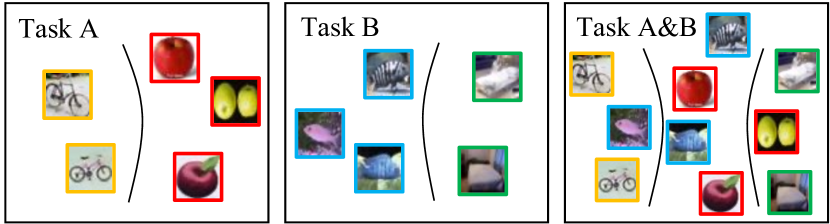
(a) inter-task confusion (ITC)

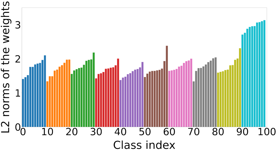
(b) old-new confusion (ONC)

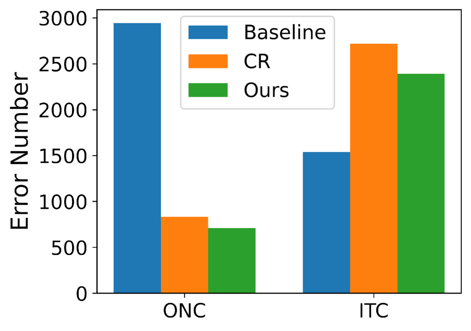
(c) error statistics

Figure 1: Task confusion illustration. (a) ITC: class discrepancy within every task is well learned, but it is not taught to distinguish classes from different tasks. (b) ONC: old classes have similar weight distribution while larger weights are given to new classes. (c) TCIL significantly reduces ONC errors on CIFAR100. It also suppresses the cases that ONC transforming to ITC to some extent (CR V.S. Ours), leading to remarkable overall confusion reduction.

However, DEAs are unable to process two kinds of confusion effectively due to their dynamically expandable nature. The first is inter-task confusion (ITC). An illustrative example is shown in Fig.1(a). Both tasks A and B are trained to distinguish their own classes. However, the discrepancy between classes from different tasks is not taught when the two tasks are combined, thus causing confusion. The second is old-new confusion (ONC). It is explained as the classifier would give priority to new classes rather than old classes. Since tasks share the same classification layer whose weights are lastly optimized by new classes, the weights are oftentimes dominated by new classes, as shown in Fig.1(b). We argue that both ITC and ONC caused by the correlation between tasks are barely investigated in DEAs.

Note that the correlation between tasks in class incremental learning has been explored in the literature (Masana et al. 2020; Wu et al. 2019; Hou et al. 2019), for example, in the form of knowledge distillation (Li and Hoiem 2017; Rebuffi et al. 2017; Douillard et al. 2020; Min et al. 2020). However, knowledge distillation does not always lead to improvements (Masana et al. 2020; Belouadah and Popescu 2019), and it is not trivial to establish due to the characteristic of DEA, which makes the correlation between tasks in DEAs less explored. Moreover, while ONC has been widely recognized as the task-tendency bias (Belouadah and Popescu 2019; Wu et al. 2019; Zhao et al. 2020), existing DEAs address it mainly by finetuning the classifier on a balanced training subset, which brings additional training burden and is highly dependent on the memory budget. Simple but effective solutions such as weight aligning (Zhao et al. 2020) have not yet been carefully investigated in DEAs. Besides, a majority of existing dynamic expansion methods are with certain prerequisites, e.g., requiring a task identifier at testing (Fernando et al. 2017; Hung et al. 2019; Wen, Tran, and Ba 2020), sensitive to rehearsal memory (Yan, Xie, and He 2021), or needing complex hyperparameter tuning (Yan, Xie, and He 2021).

Motivated by the aforementioned issues, we propose a novel framework termed as Task Correlated Incremental Learning (TCIL) that aims to mitigate catastrophic forgetting from the angle of resolving task confusion in the DEA framework. As shown in Fig.1(c), ONC is still the major error type in CIFAR100. To this end, a classifier re-scoring (CR) strategy is applied to rectify the heavily biased classification layer. Similar to (Zhao et al. 2020), it calculates the weight magnitude statistics according to old and new classes. Moreover, in contrast to previous DEAs that directly concatenate old and new features together, we design a feature fusion module to attend to the most relevant features by using the attention mechanism. With these modifications, ONC errors are largely reduced but it also causes an increase in ITC errors. Therefore, a novel multi-level knowledge distillation is developed to further deal with ITC, where knowledge propagation mechanisms are established at both feature and logit levels. Specifically, it builds information propagation paths from every old feature extractor to the new extractor, generating distillations from previous classifiers to the current classifier. It forms a complete supervision from old knowledge to the new classifier. As seen in Fig.1(c), it reduces the errors in both ITC and ONC (CR V.S. Ours). By combining all the upgrades, TCIL is capable of better handling task confusion and thus catastrophic forgetting, producing a more discriminative and fair classification. To validate the effectiveness of TCIL, we conduct extensive experiments on CIFAR100 and ImageNet100 datasets with variants such as different task splits, with or without rehearsal memory, etc. The results demonstrate that TCIL consistently achieves state-of-the-art accuracy. While TCIL-Lite, the lite version TCIL, is smaller but still effective. Moreover, compared with existing methods, TCIL is more robust as the increase of incremental steps and is less sensitive to the availability of rehearsal memory, e.g., showing greater accuracy gaps in case no rehearsal memory is kept.

Contributions of this paper can be summarized as follows. We analyze the classification error and task confusion within the DEA framework. It mainly consists of ITC and ONC. To this end, we propose TCIL, a novel scheme to promote a discriminative and fair feature utilization across tasks in class incremental Learning. Specifically, we integrate a classifier re-scoring strategy along with a feature fusion module to alleviate ONC. Meanwhile, a multi-level knowledge distillation is developed to further suppress ITC. As a result, TCIL greatly mitigates the two types of task confusion, it consistently performs top-tier and shows advantages in solving catastrophic forgetting even in non-rehearsal setting.

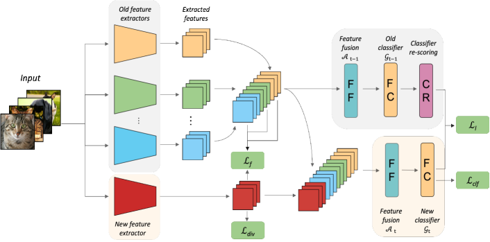
Figure 2: An illustrative framework of the proposed TCIL. It uses a dedicated feature extraction sub-network for each specific task. $\mathcal{L}_{\mathrm{f}}$ and $\mathcal{L}_{\mathrm{l}}$ are knowledge distillation loss at feature and logit levels, respectively. $\mathcal{L}_{\mathrm{clf}}$ is the classification loss, and $\mathcal{L}_{\mathrm{div}}$ is the divergence loss for guiding the training of the feature extractors.

Related Work

Catastrophic Forgetting. Many researches have been carried out to overcome catastrophic forgetting. We can broadly classify them into three categories: regularization-based (Kirkpatrick et al. 2017; Zenke, Poole, and Ganguli 2017; Dhar et al. 2019; Li and Hoiem 2017), rehearsal-based (Parisi et al. 2019; De Lange et al. 2019; Castro et al. 2018; Shin et al. 2017; Aljundi et al. 2018) and DEA-based (Fernando et al. 2017; Golkar, Kagan, and Cho 2019; Hung et al. 2019; Yan, Xie, and He 2021; Li et al. 2021; Douillard et al. 2022). Regularization-based methods emphasize on constraining the weight changes. For example, allowing only small magnitude changes on previous weights. It suffers from the problem that the changes cannot sufficiently describe the complex pattern shift caused by new task learning. Rehearsal-based methods reserve a small amount of old data when training a new task. By doing so, it retains certain previous knowledge. Studies in this category mainly focus on the selection of old data and the way to use it. For example, iCaRL was developed to learn an exemplar-based data representation (Rebuffi et al. 2017). However, rehearsal methods are difficult to scale up to a large number of classes because of the memory constraint, e.g., only a limited number of training samples could be reserved in total. Nevertheless, strategies such as generating synthetic data (Wu et al. 2018; Xiang et al. 2019) or features (Yu et al. 2020) also alleviated this dilemma.

Alternatively, DEAs choose a different way that dynamically creates feature extraction sub-networks each associated with one specific task (Fernando et al. 2017; Golkar, Kagan, and Cho 2019; Hung et al. 2019; Rusu et al. 2016; Collier et al. 2020; Wen, Tran, and Ba 2020). Early methods required a task identifier to select the right subset of parameters at test-time. Unfortunately, the assumption is unrealistic as new samples would not come with their task identifiers. Recently, DER (Yan, Xie, and He 2021) proposed a dynamically expandable representation by discarding the task identifier, where the classifier was finetuned on a balanced exemplar subset to mitigate the task-tendency bias. Li (Li et al. 2021) also proposed a multi-extractor based learning framework, where knowledge distillation and network pruning were leveraged. However, the distillation was applied to nearby tasks only. DyTox (Douillard et al. 2022) shared encoder and decoder among tasks while differentiating tasks only by special tokens. It largely reduced the network size and attained impressive results.

Knowledge Distillation. It aims to utilize a large teacher model to guide the training of a small student model (Hinton, Vinyals, and Dean 2015; Yang et al. 2022b, a). Performing the learning at logit-level is an effective and direct way of knowledge distillation (Chen et al. 2021). It is expected to distillate previous learned old knowledge to new task model in class incremental learning. LwF (Li and Hoiem 2017) first applied it to this scenario, where a modified cross-entropy loss was used to preserve the capabilities of old model. It was extended to multi-class classification scenarios later (Rebuffi et al. 2017). M2KD (Zhou et al. 2019) introduced a multi-level knowledge distillation strategy. It utilized all previous model snapshots instead of distilling knowledge only from the last model. However, it is investigated under fixed network structure. Recently, the distillation was considered from intermediate layers rather than the outputted logit, by keeping either feature map activation (Dhar et al. 2019), the spatial pooling (Douillard et al. 2020), or the normalized global pooling (Hou et al. 2019) as similar as possible. However, these methods were not well combined with the solution for task-tendency bias yet, thus restricting the classification accuracy to some extent.

Note that DEAs are different from previous incremental learning paradigms. Both the task correlation and task-tendency bias are not well investigated in the DEA framework. We formulate the issues as ITC and ONC and propose to use multi-level knowledge distillation and classifier re-scoring to address them.

Method

Problem Formulation and Method Overview

We first describe the problem investigated in the context of image classification. Assume there are $T$ batches of data $\left\{\mathcal{D}_{1},\cdots,\mathcal{D}_{T}\right\}$, with $\mathcal{D}_{t}=\left\{\left(\mathbf{x}_{1}^{t},y_{1}^{t}\right),\cdots,\left(\mathbf{x}_{n_{t}}^{t},y_{n_{t}}^{t}\right)\right\}$ as the training data at step $t$ (i.e., task $t$), where ${x}_{i}^{t}$ is the $i$-th input image and $y_{i}^{t}\in\mathcal{C}_{t}$ is the label within the label set $\mathcal{C}_{t}$, $n_{t}$ is the number of samples in set $\mathcal{D}_{t}$. At the $t$-th incremental step, training batches $t$ will be added to the training set. Therefore, the goal can be formulated as to learn knowledge from new data $\mathcal{D}_{t}$, while retain the previous knowledge learned from old data $\left\{\mathcal{D}_{1},\cdots,\mathcal{D}_{t-1}\right\}$. The label space of the model is all seen categories $\tilde{\mathcal{C}}_{t}=\cup_{i=1}^{t}\mathcal{C}_{i}$ and the model is expected to predict well on all classes in $\tilde{\mathcal{C}}_{t}$. All label sets are exclusive, i.e., $\mathcal{C}_{i}\cap\mathcal{C}_{j}=\emptyset$ for arbitrarily given $i$ and $j$. In rehearsal setting, an exemplar subset of the previous data under fixed memory budget is accessible for every incremental steps. While access to previous data is forbidden in non-rehearsal setting.

To mitigate catastrophic forgetting, we propose TCIL based on the DEA framework. Its overview is illustrated in Fig.2. As seen, a multi-level knowledge distillation is established at both feature and logit levels, i.e., $\mathcal{L}_{\mathrm{f}}$ and $\mathcal{L}_{\mathrm{l}}$. It encourages information propagation from every old task to the new task, thus alleviating ITC and ONC. Meanwhile, feature extracted from different tasks are appropriately fused to highlight these important ones. While weights of the outputted layer are adjusted to derive a more fair classification, thus mitigating ONC. The pipeline is elaborated as follows.

TCIL Architecture and Details

TCIL Pipeline. In DEAs, the feature extractor $\mathcal{F}_{1}$ and classifier $\mathcal{G}_{1}$ at the first step is trained the same as previous methods (Dhar et al. 2019; Aljundi et al. 2018; Li and Hoiem 2017; Rebuffi et al. 2017). Then at each step $t\in\left\{2,\cdots,T\right\}$, we add a new feature extractor $\mathcal{F}_{t}$ while keeping the parameters of previous extractors $\left\{\mathcal{F}_{1},\cdots,\mathcal{F}_{t-1}\right\}$ and previous classifier $\mathcal{G}_{t-1}$ frozen. Meanwhile, we initialize the parameters of $\mathcal{G}_{t}$ with $\mathcal{G}_{t-1}$. Given an image $x$ from the seen batches $\left\{1,\cdots,t\right\}$, we concatenate all extracted features $\boldsymbol{u}_{t}$ as follows:

$$\boldsymbol{u}_{t}=\left[\mathcal{F}_{1}(\boldsymbol{x}),\cdots,\mathcal{F}_{t}(\boldsymbol{x})\right]$$ (1)

The new feature extractor $\mathcal{F}_{t}$ learns from both ${D}_{t}$, the $t$-th data batch and $\boldsymbol{u}_{t-1}$, the feature representation at step $t-1$, by using the proposed feature-level knowledge distillation elaborated later. Then we get the refined features $\boldsymbol{f}_{t}$ by an attention-based feature fusion module $\mathcal{A}_{t}$ (also elaborated later) as follows:

$$\boldsymbol{f}_{t}=\mathcal{A}_{t}(\boldsymbol{u}_{t})$$ (2)

Then we feed the refined features $\boldsymbol{f}_{t}$ into the new classifier $\mathcal{G}_{t}$, and get the output logits $\boldsymbol{o}_{t}(x)$. During model training, a logit-level knowledge distillation is also applied to guide $\mathcal{G}_{t}$ preserving old knowledge.

$$\boldsymbol{o}_{t}(\boldsymbol{x})=\mathcal{G}_{t}(\boldsymbol{f}_{t})$$ (3)

While at inference, a classifier re-scoring module in the form of $\mathcal{W}_{t}$ for the new task is figured out at the end of each training step, namely:

$$\boldsymbol{o}_{t}(\boldsymbol{x})=\mathcal{W}_{t}\left(\mathcal{G}_{t}(\boldsymbol{f}_{t})\right)$$ (4)

The new model learns probability distribution from the previous step, and we can get the the prediction $\hat{y}$ for image $x$ to calculate the cross-entropy loss:

$$p_{\mathcal{G}_{t}}(\boldsymbol{y}\mid\boldsymbol{x}) =\operatorname{Softmax}\left(\boldsymbol{o}_{t}(\boldsymbol{x})\right)$$ (5)

$$\hat{y} =\arg\max p_{\mathcal{G}_{t}}(\boldsymbol{y}\mid\boldsymbol{x})$$

Multi-level Knowledge Distillation (MLKD). In rehearsal setting, let $\mathcal{R}$ be the set of reserved samples. We apply the feature-level knowledge distillation to assist the learn of $\mathcal{F}_{t}$, the new feature extractor. Specifically, given a reserved image $\boldsymbol{x}\in\mathcal{D}_{i}$, we use the $i$-th feature extractor $\mathcal{F}_{i}$ as the teacher to guide the training, the feature-level knowledge distillation loss can be represented as:

$$\mathcal{L}_{f}(\boldsymbol{x})=||\boldsymbol{F}_{t}(\boldsymbol{x})-\boldsymbol{F}_{i}(\boldsymbol{x})||_{2},$$ (6)

Then we explain how the logit-level knowledge distillation is formulated. For each training image $\boldsymbol{x}$ we can get $\boldsymbol{o}_{t}(\boldsymbol{x})$ and $\boldsymbol{o}_{t-1}(\boldsymbol{x})$, the outputs of classifiers $\mathcal{G}_{t}$ and $\mathcal{G}_{t-1}$, respectively. Then, we use KL divergence (Passalis, Tzelepi, and Tefas 2020) to calculate the distance between them:

$$\mathcal{L}_{l}(\boldsymbol{x})=\sum_{c=1}^{\tilde{\mathcal{C}}_{t-1}}{q}_{c}(\boldsymbol{x})\log\left(\frac{{q}_{c}(\boldsymbol{x})}{\hat{q}_{c}(\boldsymbol{x})}\right),$$ (7)

where $\hat{q}_{c}(\boldsymbol{x})=\frac{e^{\hat{o}_{c}(x)/T}}{\sum_{j=1}^{\tilde{\mathcal{C}}_{t-1}}e^{\hat{o}_{j}(x)/T}}$, $q_{c}(\boldsymbol{x})=\frac{e^{o_{c}(x)/T}}{\sum_{j=1}^{\tilde{\mathcal{C}}_{t-1}}e^{o_{j}(x)/T}}$, $T$ is the temperature scalar. $\hat{o}_{c}(x)$ is an element of $\boldsymbol{o}_{t-1}(\boldsymbol{x})$, $\boldsymbol{o}_{t-1}(\boldsymbol{x})=(\hat{o}_{1}(\boldsymbol{x}),\cdots,\hat{o}_{\tilde{\mathcal{C}}_{t-1}}(\boldsymbol{x}))^{T}$ represents the logits of $\mathcal{G}_{t-1}$. $o_{c}(x)$ is an element of $\boldsymbol{o}_{t}(\boldsymbol{x})$, $\boldsymbol{o}_{t}(\boldsymbol{x})=(o_{1}(\boldsymbol{x}),\cdots,o_{\tilde{\mathcal{C}}_{t-1}}(\boldsymbol{x}),o_{\tilde{\mathcal{C}}_{t-1}+1}(\boldsymbol{x}),\cdots,o_{\tilde{\mathcal{C}}_{t}}(\boldsymbol{x}))^{T}$ stands for the logits of $\mathcal{G}_{t}$. Then, parameters of both feature extractor $\mathcal{F}_{t}$ and classifier $\mathcal{G}_{t}$ are updated with the combined loss during training. The total loss can be written as:

$$\mathcal{L}_{\mathrm{kd}}=\lambda\sum_{\boldsymbol{x}\in\mathcal{R}}\mathcal{L}_{f}(\boldsymbol{x})+\mu\sum_{\boldsymbol{x}\in\mathcal{R}\cup\mathcal{D}_{t}}\mathcal{L}_{l}(\boldsymbol{x}),$$ (8)

where $\lambda$ and $\mu$ are hyperparameters both empirically set to 0.5. $\lambda=0$ means the non-rehearsal setting, i.e., all loss is from $\mathcal{L}_{l}$.

Methods	CIFAR100-B0									CIFAR100-B50
	5 steps			10 steps			20 steps			2 steps			5 steps			10 steps
	#Paras	Avg	Last	#Paras	Avg	Last	#Paras	Avg	Last	#Paras	Avg	Last	#Paras	Avg	Last	#Paras	Avg	Last
Bound	11.2	80.40	-	11.2	80.41	-	11.2	81.49	-	11.2	77.20	-	11.2	79.89	-	11.2	79.91	-
iCaRL (2017)	11.2	71.14	59.71	11.2	65.27	50.74	11.2	61.20	43.75	11.2	77.20	-	11.2	79.89	-	11.2	79.91	-
UCIR (2019)	11.2	62.77	47.31	11.2	58.66	43.39	11.2	58.17	40.63	11.2	67.21	56.82	11.2	64.28	52.02	11.2	59.92	48.02
BiC (2019)	11.2	73.10	62.1	11.2	68.80	53.54	11.2	66.48	47.02	11.2	72.47	64.22	11.2	66.62	55.01	11.2	60.25	48.04
RPSNet (2019)	60.6	70.50	60.56	56.5	68.60	57.05	-	-	-	-	-	-	-	-	-	-	-	-
WA (2020)	11.2	72.81	60.84	11.2	69.46	53.78	11.2	67.33	47.31	11.2	71.43	62.37	11.2	64.01	52.87	11.2	57.86	47.90
PODNet (2020)	11.2	66.70	51.71	11.2	58.03	41.05	11.2	53.97	35.02	11.2	71.30	62.11	11.2	67.25	55.94	11.2	64.04	52.13
DER (2021)	33.6	76.80	68.32	61.6	75.36	65.22	117.6	74.09	62.48	22.4	74.61	68.84	39.2	73.21	65.77	67.2	72.81	65.45
DyTox (2022)	-	-	-	10.7	73.66	60.67	10.7	72.27	56.32	-	-	-	-	-	-	-	-	-
TCIL	34.3	77.72	69.58	64.1	77.30	66.41	127.1	75.11	63.54	22.7	76.42	71.91	40.2	74.88	68.58	70.3	73.72	66.36
TCIL-Lite	8.3	76.96	69.44	14.5	76.74	66.66	28.1	75.47	64.08	5.4	74.95	70.72	8.3	74.30	68.89	14.5	73.50	67.26

Table 1: Top-1 accuracy comparison on CIFAR100 in rehearsal setting. Dytox (Douillard et al. 2022) and RPSNet (Rajasegaran et al. 2019) results come from their respective papers, and other results come from  (Yan, Xie, and He 2021).

Classifier Re-scoring (CR). When the step $t>1$, ONC appears as $\mathcal{G}_{t}$ is biased to new classes. Similar to (Zhao et al. 2020), we propose to re-score the old and new classes based on their weight norms. To be specific, at the end of each training step, we calculate the weight norms of old classes and new classes in the last fully connected layer as follows:

$$\boldsymbol{n}_{old} =\left(\left\|\mathbf{w}_{1}\right\|,\cdots,\left\|\mathbf{w}_{\tilde{\mathcal{C}}_{t-1}}\right\|\right),$$ (9)

$$\boldsymbol{n}_{new} =\left(\left\|\mathbf{w}_{\tilde{\mathcal{C}}_{t-1}+1}\right\|,\cdots,\left\|\mathbf{w}_{\tilde{\mathcal{C}}_{t}}\right\|\right)$$

Based on the above norms, we calculate the coefficient $\gamma$ for classifier re-scoring:

$$\gamma={\operatorname{Mean}\left(\boldsymbol{n}_{{old}}\right)}/{\operatorname{Mean}\left(\boldsymbol{n}_{{new}}\right)}$$ (10)

where $\operatorname{Mean(\cdot)}$ returns the mean value of elements in the vector. We rewrite the output logits $\boldsymbol{o}_{rt}(\boldsymbol{x})$ in the following form: $\boldsymbol{o}(\boldsymbol{x})=(\boldsymbol{o}_{t-1}(\boldsymbol{x}),\boldsymbol{o}_{t}(\boldsymbol{x})[\tilde{\mathcal{C}}_{t-1}+1,\dots,\tilde{\mathcal{C}}_{t}])$, where $\boldsymbol{o}_{t}(\boldsymbol{x})$ indicates the logits of $\mathcal{G}_{t}$. Then the rectified logits $\boldsymbol{o}(\boldsymbol{x})$ is given by:

$$\boldsymbol{o}_{rt}(\boldsymbol{x})=\mathcal{W}_{t}(\boldsymbol{o}(\boldsymbol{x}))=\left(\mathbf{o}_{old}(\boldsymbol{x}),\gamma\cdot\boldsymbol{o}_{new}(\boldsymbol{x})\right)$$ (11)

By doing this, the average norm of outputted logits for new classes becomes the same as those of the old classes, thus well mitigating ONC. Note that within new classes (or old classes), the relative magnitude of logits does not change.

Feature Fusion Module (FFM). Considering that feature extractors $\left\{\mathcal{F}_{1},\cdots,\mathcal{F}_{t-1}\right\}$ are trained at different steps and they could not extract features of images from new steps $\left\{t,\cdots,\mathcal{T}\right\}$ well, which affects the quality of features, we apply FFM to refine the features and combine the transformed features for classification. Given an intermediate feature map $\boldsymbol{u}_{t}\in\mathbb{R}^{C\times H\times W}$ as input, similar to  (Woo et al. 2018), FFM sequentially infers a 1D attention map $\mathbf{A}_{\mathbf{c}}\in\mathbb{R}^{C\times 1\times 1}$ and a 2D attention map $\mathbf{A}_{\mathbf{s}}\in\mathbb{R}^{1\times H\times W}$. The whole feature fusion process can be summarized as:

$$\boldsymbol{f}_{t}=\mathcal{A}_{t}(\boldsymbol{u}_{t}) =\mathbf{A}_{\mathbf{s}}\left(\mathbf{A}_{\mathbf{c}}(\boldsymbol{u}_{t})\otimes\boldsymbol{u}_{t}\right)\otimes\left(\mathbf{A}_{\mathbf{c}}(\boldsymbol{u}_{t})\otimes\boldsymbol{u}_{t}\right)$$ (12)

where $\otimes$ denotes element-wise multiplication. Therefore, $\mathbf{A}_{\mathbf{c}}$ and $\mathbf{A}_{\mathbf{s}}$ are the channel attention (Hu, Shen, and Sun 2018; Woo et al. 2018; Li et al. 2019) and spatial attention (Woo et al. 2018; Wang et al. 2018) defined as follows.

$$\mathbf{A}_{\mathbf{c}}(\boldsymbol{u}_{t}) =\sigma(MLP(\operatorname{Avg}\operatorname{Pool}(\boldsymbol{u}_{t}))+MLP(\operatorname{Max}\operatorname{Pool}(\boldsymbol{u}_{t})))$$ (13)

$$\mathbf{A}_{\mathbf{s}}(\boldsymbol{u}_{t}) =\sigma\left(f^{7\times 7}([\operatorname{Avg}\operatorname{Pool}(\boldsymbol{u}_{t});\operatorname{Max}\operatorname{Pool}(\boldsymbol{u}_{t})])\right)$$ (14)

where $\sigma$ denotes the sigmoid function and $f^{7\times 7}$ represents a convolution with kernel size of $7\times 7$. During multiplication, the attention values are broadcasted accordingly.

Training Loss. TCIL is trained with three losses, i.e., the classification loss $\mathcal{L}_{clf}$ calculated by cross-entropy, the multi-level knowledge distillation loss given by Eq.8, and a divergence loss $\mathcal{L}_{\mathrm{div}}$ to maximum the discrepancy between old-new classes as in (Yan, Xie, and He 2021). Formally, the total loss is:

$$\mathcal{L}=\mathcal{L}_{\mathrm{clf}}+\alpha\mathcal{L}_{\mathrm{kd}}+\beta\mathcal{L}_{\mathrm{div}},$$ (15)

where $\alpha$ and $\beta$ are hyperparameters both empirically set to 1.0 for all experiments.

Note that the proposed multi-level knowledge distillation significantly enriches the use of previous old knowledge. It not only establishes information propagation paths from every old feature extractor to the new extractor at the feature level, but also enables the information sharing from the old classifier to the new one at the logit level, thus forming a multi-grained distillation that has not been proposed before. In addition, the re-scoring strategy is also applied for the first time to the DEA framework.

Network Pruning

Since feature extraction sub-networks are sequentially added with new tasks, TCIL parameters grow with the incremental steps, which is undesired in real-world applications. As a solution, we devise TCIL-Lite, the lite version TCIL, by applying parameter pruning techniques described in (He et al. 2019). Instead of pruning small convolution kernels, it calculates the geometric median (Fletcher, Venkatasubramanian, and Joshi 2008) between the kernels. Then kernel pairs whose similarity above a threshold are treated as redundant and one of them is pruned. With this strategy, the model size could be largely reduced while not affecting the accuracy too much. Since pruning is not the emphasis of this paper, we empirically set TCIL-Lite nearly four times smaller than TCIL. We will demonstrate the effectiveness of TCIL-Lite in the experiments.

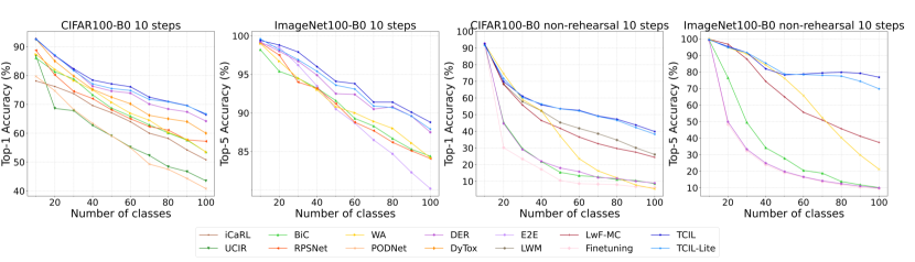
Figure 3: Accuracy evolution on benchmarks. The left are evaluated on CIFAR100-B0 and ImageNet100-B0 with 10 steps in rehearsal setting. The right are evaluated on CIFAR100-B0 and ImageNet100-B0 with 10 steps in non-rehearsal setting.

Experiments

Implementation

To evaluate TCIL, we conduct extensive experiments on CIFAR100 (Krizhevsky 2009) and ImageNet100 (Russakovsky et al. 2015) under two memory settings: fixed exemplar memory (rehearsal) and none exemplar memory (non-rehearsal). In rehearsal setting, following (Douillard et al. 2022; Yan, Xie, and He 2021; Rebuffi et al. 2017; Douillard et al. 2020), we set the memory size to 2000 images. For CIFAR100, two protocols are considered. The first is CIFAR100-B0: training all 100 classes from scratch with different task splits, i.e., 5, 10 and 20 incremental steps. The second is CIFAR100-B50: starting from a model trained on 50 classes, and the remaining 50 classes are divided into splits of 2, 5 and 10 steps. We report the top-1 accuracy both averaged over the incremental steps (Avg) and after the last step (Last). For ImageNet100, we assess our methods on the ImageNet100-B0 protocol: the model is trained in batches of 10 classes from scratch and uses the same ImageNet subset and class order following (Douillard et al. 2020; Hou et al. 2019; Rebuffi et al. 2017; Yan, Xie, and He 2021). Both top-1 and top-5 accuracy is reported. While in non-rehearsal setting, we evaluate TCIL on both CIFAR100-B0 and ImageNet100-B0 protocols.

Following (Li et al. 2021; Yan, Xie, and He 2021), we adopt ResNet-18 as the basic network for feature extraction. For CIFAR100, we employ random crop and horizontal flip as the data augmentation. While for ImageNet100, we employ the data augmentation in (Mittal, Galesso, and Brox 2021). Data augmentation like rotation, brightness variation and cutout, are randomly performed during the training. We adopt SGD optimizer with weight decay 0.0005 and batch size 128 for all experiments. We use the warmup strategy with the ending learning rate 0.1 for 10 epochs in CIFAR100 and 20 epochs in ImageNet100, respectively. After the warmup, for CIFAR100 the learning rate is 0.1 and decays to 0.01 and 0.001 at 100 and 120 epochs. For ImageNet100 the learning rate decays to 0.01, 0.001 and 0.0001 at 60, 120 and 180 epochs. In rehearsal setting, we use the same exemplar selection strategy as (Rebuffi et al. 2017; Hou et al. 2019). All models are trained by using a workstation with 1 Nvidia 3090 GPU on Pytorch.

	ImageNet100-B0
	top-1			top-5
Methods	#Paras	Avg	Last	Avg	Last
Bound	11.2	-	-	95.10	-
iCaRL (2017)	11.2	-	-	83.60	63.80
E2E (2018)	11.2	-	-	89.92	80.29
BiC (2019)	11.2	-	-	90.60	84.40
RPSNet (2019)	-	-	-	87.90	74.00
WA (2020)	11.2	-	-	91.00	84.10
DER (2021)	61.6	77.18	66.70	93.23	87.52
DyTox (2022)	11.0	77.15	69.10	92.04	87.98
TCIL	64.1	77.66	67.34	94.17	88.84
TCIL-Lite	14.5	77.50	67.30	93.60	87.94

Table 2: Top-1 and top-5 accuracy comparison on ImageNet100-B0 in rehearsal setting.

Results and Discussion

Rehearsal Setting. The results on CIFAR100 and ImageNet100 with different protocols are given in Tab.1 and Tab.2, respectively. In both CIFAR100-B0 and CIFAR100-B50, DEA-based models (e.g., DER, DyTox and TCIL) outperform non-DEA-based models by large margins at all task splits. They also exhibit smaller accuracy decline with the accumulation of incremental steps, showing the effectiveness of DEA-based methods in reducing the forgetting of old knowledge. When looking into DEA-based models, TCIL gains certain accuracy improvements but with increased model size, especially compared with DyTox. However, TCIL-Lite largely alleviates this dilemma. Although slightly inferior to TCIL at small steps (i.e., 2 or 5 steps), TCIL-Lite gradually approaches and even outperforms TCIL with the increase of incremental steps, indicating that the pruning almost does not affect the network capability in rehearsal setting. Moreover, when compared with DER, the previous leading method in the DEA family, TCIL-Lite consistently has better accuracy and fewer parameters. Note that similar comparison results are also observed in ImageNet100-B0, TCIL and TCIL-Lite suppress existing models in most cases. In Fig.3, four line charts with different configurations are depicted to show the detailed accuracy evolution with the incremental steps (More line charts are given in the supplement). TCIL and TCIL-Lite are always with the slowest forgetting rate and ranking top-tier. The results clearly demonstrate the superiority of TCIL in rehearsal setting.

Methods	CIFAR100 B0						ImageNet100-B0
	5 steps			10 steps			10 steps
	#Paras	Avg	Last	#Paras	Avg	Last	#Paras	Avg	Last
Finetuning	11.2	32.89	11.42	11.2	20.71	6.36	11.2	28.48	9.48
LwF-MC (2017)	-	54.74	35.42	-	45.08	24.42	-	65.45	37.42
BiC (2019)	11.2	39.31	16.70	11.2	25.47	8.57	11.2	36.24	10.02
LwM (2019)	-	63.67	49.36	-	45.68	26.14	-	-	-
WA (2020)	11.2	59.14	30.61	11.2	37.58	5.53	11.2	65.52	21.18
DER (2021)	33.6	39.93	17.31	61.6	26.53	8.88	61.6	29.15	9.96
TCIL	34.3	63.92	53.08	64.1	56.57	39.91	64.1	84.05	76.82
TCIL-Lite	8.3	63.72	51.82	14.5	56.18	38.34	14.5	82.81	69.80

Table 3: Accuracy comparison on CIFAR100 and ImageNet100 in non-rehearsal setting. LwM and LwF-MC results come from (Dhar et al. 2019). Other results are reported based on open source codes or our implementation.

		CIFAR100-B0									CIFAR100-B50									ImageNet100-B0
		5 steps			10 steps			20 steps			2 steps			5 steps			10 steps			10 steps
Methods		2000	1000	0	2000	1000	0	2000	1000	0	2000	1000	0	2000	1000	0	2000	1000	0	2000	1000	0
	Avg	76.80	73.67	39.93	75.36	71.10	26.53	74.09	70.34	16.96	74.61	72.50	43.89	73.21	70.17	23.31	72.81	69.67	13.11	93.23	78.06	29.15
DER (2021)	Last	68.32	62.22	17.31	65.22	56.77	8.88	62.48	53.32	4.80	68.84	64.70	21.45	73.21	59.99	8.85	65.45	56.98	4.80	87.52	53.96	9.96
	Avg	77.72	75.64	63.92	77.30	74.13	56.57	75.11	71.85	46.74	76.42	75.17	65.78	74.88	74.34	63.18	73.72	71.91	47.52	94.17	93.66	84.05
TCIL	Last	69.58	67.00	53.08	66.41	62.87	39.91	63.54	59.07	27.11	71.91	70.38	54.85	74.88	67.90	45.39	66.36	64.79	255.4	88.84	86.04	76.82

Table 4: Accuracy comparison with different memory budget (number of exemplars). We report the top-1 accuracy on CIFAR100 and the top-5 accuracy on ImageNet100.

Non-Rehearsal Setting. Table 3 shows the results on CIFAR100-B0 and ImageNet100-B0 with different incremental steps. The results are generally worse than those with the rehearsal memory and experience even sharp decreases as the increase of incremental steps, showing the positive effect of reserving certain old data. When comparing existing models, TCIL surpasses LwM, the previous state of the art, by 3.72% and 13.7% at ”Last” on CIFAR100-B0 with 5 and 10 steps, respectively. Moreover, TCIL outperforms DER by significant larger margins compared to the rehearsal case. It implies that TCIL is less sensitive to the availability of rehearsal memory, which is an advantage in many applications. Compared TCIL with TCIL-Lite, TCIL is more robust as the step accumulated. It can be explained as the generalization ability of TCIL-Lite is worse in challenging cases due to the limited network capacity. In non-rehearsal scenario, TCIL only distills from the outputted logits, where much less knowledge could be dug. Nevertheless, TCIL-Lite still performs significantly better than DER in all the listed protocols while with few parameters. The observations reveal advantages of the TCIL family from another angle and again demonstrate their effectiveness.

DEA	Div Loss	CR	MLKD	FFM	Avg
					61.84
✓					69.45
✓	✓				70.59
✓	✓	✓			73.43
✓	✓	✓	✓		75.80
✓	✓	✓	✓	✓	77.30

Table 5: Ablations on the components of TCIL

Ablation Study and Error Analysis

We ablate the components in TCIL to validate their utilities and Tab. 5 give the result, where ResNet-18 with 10 incremental steps and the rehearsal strategy is taken as the baseline. First, equipping the DEA generates 7.61% accuracy gains. Then, applying the divergence loss to encourage feature extractors to better distinguish between old-new classes gives marginal improvements. In the following, applying CR and MLKD further gives 2.84% and 2.37% accuracy improvements, indicating that the two upgrades are good at suppressing task confusion in the DEA framework. Finally, FFM also reports an improvement of 1.5% by injecting the combined attention mechanism. The ablation basically verifies the effectiveness of the employed components.

To analyze the task confusion within DEAs, we perform experiments on CIFAR100-B0 with 10 incremental steps and group the errors into three types, i.e., ITC, ONC and within-task confusion (WTC). ResNet-18 with DEA and rehearsal strategy are employed as the baseline, i.e., the second line in Tab. 5. While CR and TCIL are compared, which correspond to the fourth and sixth lines in Tab. 5, respectively. Task confusion in the form of error statistics are summarized in Tab. 6. As can be seen, the three methods gradually exhibit differences with the increase of steps. ONC errors have been reduced significantly by applying CR. However, it also leads to an increase of ITC errors. We argue that these newly added ITC errors are samples that are prone to ONC, and were previously classified as ONC errors due to severe task-tendency bias in the baseline. Nevertheless, compared to CR, TCIL further reduces all three kinds of errors. These results intuitively show that TCIL can effectively reduce task confusion by mitigating ONC and ITC in a targeted manner. On the other hand, WTC errors account for a small proportion of the total number of errors, less than 10% at the last step. This result indicates that ITC and ONC are the main cause of catastrophic forgetting, which is different from the case of fixed network structure that often suffers from weight drift (Aljundi et al. 2018; Kirkpatrick et al. 2017). Our exploration basically verifies that to address the catastrophic forgetting in DEAs, more attention needs to be paid to the task confusion, especially ITC and ONC.

Methods	Error	Incremental tasks
		1	2	3	4	5	6	7	8	9	10
baseline	WTC	75	133	169	164	191	169	226	182	207	254
	ONC	0	162	450	750	856	1034	1597	1834	2053	2943
	ITC	0	0	67	237	524	794	824	1200	1481	1538
CR	WTC	75	132	173	169	199	194	232	228	248	271
	ONC	0	170	390	583	541	515	739	743	647	832
	ITC	0	0	75	291	670	1023	1249	1733	2254	2718
TCIL	WTC	75	120	157	177	212	211	223	221	238	248
	ONC	0	141	284	382	309	345	538	476	453	709
	ITC	0	0	92	309	630	879	1156	1619	2046	2391

Table 6: Error statistics on CIFAR100-B0. ITC, ONC, WTC denote inter-task confusion, old-new confusion, within-task confusion, respectively.

,

We set up a controlled trial with DER to illustrate TCIL is much less dependent on rehearsal. It is clearly shown in Tab. 4 that as the memory size decreases, the gap between TCIL and DER in accuracy becomes larger no matter the dataset, evaluation protocols and task splits. The result strongly demonstrates that TCIL proposed in this paper can alleviate the problem that DER relies much on the rehearsal mechanism under the structure of dynamic extension.

Conclusion

We have inspected class incremental learning from the task confusion angle, where ITC and ONC have been pointed out as two major causes of catastrophic forgetting in DEAs. As a consequence, TCIL is presented. It develops a multi-level knowledge distillation to promote knowledge propagation and utilization, while attention mechanism and classifier re-scoring strategy are also taken into account. The experiments conducted on CIFAR100 and ImageNet100 basically verify our proposal. TCIL and TCIL-lite consistently report state-of-the-art accuracy. They are also more robust with the accumulation of incremental steps and less sensitive to the availability of rehearsal memory. The error statistics imply that task confusion is largely reduced by TCIL especially ONC errors. The strength of error reduction, though, is still limited by the fact that the knowledge in different sub-networks is still not being enough shared and fused. Thus, future work includes the exploration of more effective knowledge sharing and utilization protocols. Meanwhile, we are also interested in extending TCIL to other research scenarios, e.g., the label sets are not exclusive.

References

- Aljundi et al. (2018) Aljundi, R.; Babiloni, F.; Elhoseiny, M.; Rohrbach, M.; and Tuytelaars, T. 2018. Memory aware synapses: Learning what (not) to forget. In Proceedings of the European Conference on Computer Vision, 139–154.
- Belouadah and Popescu (2019) Belouadah, E.; and Popescu, A. 2019. Il2m: Class incremental learning with dual memory. In Proceedings of the IEEE/CVF International Conference on Computer Vision, 583–592.
- Castro et al. (2018) Castro, F. M.; Marín-Jiménez, M. J.; Guil, N.; Schmid, C.; and Alahari, K. 2018. End-to-end incremental learning. In Proceedings of the European conference on computer vision, 233–248.
- Chen et al. (2021) Chen, P.; Liu, S.; Zhao, H.; and Jia, J. 2021. Distilling knowledge via knowledge review. In Proceedings of the IEEE/CVF Conference on Computer Vision and Pattern Recognition, 5008–5017.
- Collier et al. (2020) Collier, M.; Kokiopoulou, E.; Gesmundo, A.; and Berent, J. 2020. Routing networks with co-training for continual learning. arXiv preprint arXiv:2009.04381.
- De Lange et al. (2019) De Lange, M.; Aljundi, R.; Masana, M.; Parisot, S.; Jia, X.; Leonardis, A.; Slabaugh, G.; and Tuytelaars, T. 2019. Continual learning: A comparative study on how to defy forgetting in classification tasks. arXiv preprint arXiv:1909.08383, 2(6).
- Dhar et al. (2019) Dhar, P.; Singh, R. V.; Peng, K.-C.; Wu, Z.; and Chellappa, R. 2019. Learning without memorizing. In Proceedings of the IEEE/CVF Conference on Computer Vision and Pattern Recognition, 5138–5146.
- Douillard et al. (2020) Douillard, A.; Cord, M.; Ollion, C.; Robert, T.; and Valle, E. 2020. Podnet: Pooled outputs distillation for small-tasks incremental learning. In European Conference on Computer Vision, 86–102. Springer.
- Douillard et al. (2022) Douillard, A.; Ramé, A.; Couairon, G.; and Cord, M. 2022. Dytox: Transformers for continual learning with dynamic token expansion. In Proceedings of the IEEE/CVF Conference on Computer Vision and Pattern Recognition, 9285–9295.
- Fernando et al. (2017) Fernando, C.; Banarse, D.; Blundell, C.; Zwols, Y.; Ha, D.; Rusu, A. A.; Pritzel, A.; and Wierstra, D. 2017. Pathnet: Evolution channels gradient descent in super neural networks. arXiv preprint arXiv:1701.08734.
- Fletcher, Venkatasubramanian, and Joshi (2008) Fletcher, P. T.; Venkatasubramanian, S.; and Joshi, S. 2008. Robust statistics on Riemannian manifolds via the geometric median. In IEEE Conference on Computer Vision and Pattern Recognition, 1–8. IEEE.
- Golkar, Kagan, and Cho (2019) Golkar, S.; Kagan, M.; and Cho, K. 2019. Continual learning via neural pruning. arXiv preprint arXiv:1903.04476.
- Goodfellow et al. (2013) Goodfellow, I. J.; Mirza, M.; Xiao, D.; Courville, A.; and Bengio, Y. 2013. An Empirical Investigation of Catastrophic Forgetting in Gradient-Based Neural Networks. Computer Science, 84(12): 1387–91.
- He et al. (2019) He, Y.; Liu, P.; Wang, Z.; Hu, Z.; and Yang, Y. 2019. Filter pruning via geometric median for deep convolutional neural networks acceleration. In Proceedings of the IEEE/CVF Conference on Computer Vision and Pattern Recognition, 4340–4349.
- Hinton, Vinyals, and Dean (2015) Hinton, G.; Vinyals, O.; and Dean, J. 2015. Distilling the Knowledge in a Neural Network. Computer Science, 14(7): 38–39.
- Hou et al. (2019) Hou, S.; Pan, X.; Loy, C. C.; Wang, Z.; and Lin, D. 2019. Learning a unified classifier incrementally via rebalancing. In Proceedings of the IEEE/CVF Conference on Computer Vision and Pattern Recognition, 831–839.
- Hu, Shen, and Sun (2018) Hu, J.; Shen, L.; and Sun, G. 2018. Squeeze-and-excitation networks. In Proceedings of the IEEE conference on computer vision and pattern recognition, 7132–7141.
- Hung et al. (2019) Hung, C.-Y.; Tu, C.-H.; Wu, C.-E.; Chen, C.-H.; Chan, Y.-M.; and Chen, C.-S. 2019. Compacting, picking and growing for unforgetting continual learning. Advances in Neural Information Processing Systems, 32.
- Kirkpatrick et al. (2017) Kirkpatrick, J.; Pascanu, R.; Rabinowitz, N.; Veness, J.; Desjardins, G.; Rusu, A. A.; Milan, K.; Quan, J.; Ramalho, T.; Grabska-Barwinska, A.; et al. 2017. Overcoming catastrophic forgetting in neural networks. Proceedings of the national academy of sciences, 114(13): 3521–3526.
- Krizhevsky (2009) Krizhevsky, A. 2009. Learning Multiple Layers of Features from Tiny Images. Master’s thesis, University of Tront.
- Lange et al. (2020) Lange, M. D.; Jia, X.; Parisot, S.; Leonardis, A.; Slabaugh, G.; and Tuytelaars, T. 2020. Unsupervised model personalization while preserving privacy and scalability: An open problem. In Proceedings of the IEEE/CVF Conference on Computer Vision and Pattern Recognition, 14463–14472.
- Li et al. (2017) Li, L.; Jun, Z.; Fei, J.; and Li, S. 2017. An incremental face recognition system based on deep learning. In 2017 Fifteenth IAPR International Conference on Machine Vision Applications (MVA), 238–241.
- Li et al. (2019) Li, X.; Wang, W.; Hu, X.; and Yang, J. 2019. Selective kernel networks. In Proceedings of the IEEE/CVF Conference on Computer Vision and Pattern Recognition, 510–519.
- Li and Hoiem (2017) Li, Z.; and Hoiem, D. 2017. Learning without forgetting. IEEE transactions on pattern analysis and machine intelligence, 40(12): 2935–2947.
- Li et al. (2021) Li, Z.; Zhong, C.; Liu, S.; Wang, R.; and Zheng, W.-S. 2021. Preserving earlier knowledge in continual learning with the help of all previous feature extractors. arXiv preprint arXiv:2104.13614.
- Lu et al. (2022) Lu, Z.; Xie, H.; Liu, C.; and Zhang, Y. 2022. Bridging the Gap Between Vision Transformers and Convolutional Neural Networks on Small Datasets. In Advances in Neural Information Processing Systems.
- Masana et al. (2020) Masana, M.; Liu, X.; Twardowski, B.; Menta, M.; Bagdanov, A. D.; and van de Weijer, J. 2020. Class-incremental learning: survey and performance evaluation on image classification. arXiv preprint arXiv:2010.15277.
- Min et al. (2020) Min, S.; Yao, H.; Xie, H.; Zha, Z.-J.; and Zhang, Y. 2020. Multi-objective matrix normalization for fine-grained visual recognition. IEEE Transactions on Image Processing, 29: 4996–5009.
- Mittal, Galesso, and Brox (2021) Mittal, S.; Galesso, S.; and Brox, T. 2021. Essentials for class incremental learning. In Proceedings of the IEEE/CVF Conference on Computer Vision and Pattern Recognition, 3513–3522.
- Parisi et al. (2019) Parisi, G. I.; Kemker, R.; Part, J. L.; Kanan, C.; and Wermter, S. 2019. Continual lifelong learning with neural networks: A review. Neural Networks, 113: 54–71.
- Passalis, Tzelepi, and Tefas (2020) Passalis, N.; Tzelepi, M.; and Tefas, A. 2020. Probabilistic knowledge transfer for lightweight deep representation learning. IEEE Transactions on Neural Networks and Learning Systems, 32(5): 2030–2039.
- Pierre (2018) Pierre, J. M. 2018. Incremental lifelong deep learning for autonomous vehicles. In 2018 21st international conference on intelligent transportation systems, 3949–3954. IEEE.
- Rajasegaran et al. (2019) Rajasegaran, J.; Hayat, M.; Khan, S.; Khan, F. S.; Shao, L.; and Yang, M.-H. 2019. An adaptive random path selection approach for incremental learning. arXiv preprint arXiv:1906.01120.
- Rebuffi et al. (2017) Rebuffi, S.-A.; Kolesnikov, A.; Sperl, G.; and Lampert, C. H. 2017. icarl: Incremental classifier and representation learning. In Proceedings of the IEEE conference on Computer Vision and Pattern Recognition, 2001–2010.
- Russakovsky et al. (2015) Russakovsky, O.; Deng, J.; Su, H.; Krause, J.; Satheesh, S.; Ma, S.; Huang, Z.; Karpathy, A.; Khosla, A.; Bernstein, M.; et al. 2015. Imagenet large scale visual recognition challenge. International journal of computer vision, 115(3): 211–252.
- Rusu et al. (2016) Rusu, A. A.; Rabinowitz, N. C.; Desjardins, G.; Soyer, H.; Kirkpatrick, J.; Kavukcuoglu, K.; Pascanu, R.; and Hadsell, R. 2016. Progressive neural networks. arXiv preprint arXiv:1606.04671.
- Shin et al. (2017) Shin, H.; Lee, J. K.; Kim, J.; and Kim, J. 2017. Continual learning with deep generative replay. In Advances in neural information processing systems, 2994–3003.
- Thrun (1995) Thrun, S. 1995. Is learning the n-th thing any easier than learning the first? Advances in neural information processing systems, 8.
- Wang et al. (2018) Wang, H.; Fan, Y.; Wang, Z.; Jiao, L.; and Schiele, B. 2018. Parameter-free spatial attention network for person re-identification. arXiv preprint arXiv:1811.12150.
- Wen, Tran, and Ba (2020) Wen, Y.; Tran, D.; and Ba, J. 2020. Batchensemble: an alternative approach to efficient ensemble and lifelong learning. arXiv preprint arXiv:2002.06715.
- Woo et al. (2018) Woo, S.; Park, J.; Lee, J.-Y.; and Kweon, I. S. 2018. Cbam: Convolutional block attention module. In Proceedings of the European conference on computer vision, 3–19.
- Wu et al. (2018) Wu, C.; Herranz, L.; Liu, X.; van de Weijer, J.; Raducanu, B.; et al. 2018. Memory replay gans: Learning to generate new categories without forgetting. Advances in Neural Information Processing Systems, 31.
- Wu et al. (2019) Wu, Y.; Chen, Y.; Wang, L.; Ye, Y.; Liu, Z.; Guo, Y.; and Fu, Y. 2019. Large scale incremental learning. In Proceedings of the IEEE/CVF Conference on Computer Vision and Pattern Recognition, 374–382.
- Xiang et al. (2019) Xiang, Y.; Fu, Y.; Ji, P.; and Huang, H. 2019. Incremental learning using conditional adversarial networks. In Proceedings of the IEEE/CVF International Conference on Computer Vision, 6619–6628.
- Yan, Xie, and He (2021) Yan, S.; Xie, J.; and He, X. 2021. Der: Dynamically expandable representation for class incremental learning. In Proceedings of the IEEE/CVF Conference on Computer Vision and Pattern Recognition, 3014–3023.
- Yang et al. (2022a) Yang, D.; Zhou, Y.; Shi, W.; Wu, D.; and Wang, W. 2022a. RD-IOD: Two-Level Residual-Distillation-Based Triple-Network for Incremental Object Detection. ACM Transactions on Multimedia Computing, Communications, and Applications (TOMM), 18(1): 1–23.
- Yang et al. (2022b) Yang, D.; Zhou, Y.; Zhang, A.; Sun, X.; Wu, D.; Wang, W.; and Ye, Q. 2022b. Multi-view correlation distillation for incremental object detection. Pattern Recognition, 131: 108863.
- Yu et al. (2020) Yu, L.; Twardowski, B.; Liu, X.; Herranz, L.; Wang, K.; Cheng, Y.; Jui, S.; and Weijer, J. v. d. 2020. Semantic drift compensation for class-incremental learning. In Proceedings of the IEEE/CVF Conference on Computer Vision and Pattern Recognition, 6982–6991.
- Zenke, Poole, and Ganguli (2017) Zenke, F.; Poole, B.; and Ganguli, S. 2017. Continual learning through synaptic intelligence. In International Conference on Machine Learning, 3987–3995. PMLR.
- Zhao et al. (2020) Zhao, B.; Xiao, X.; Gan, G.; Zhang, B.; and Xia, S.-T. 2020. Maintaining discrimination and fairness in class incremental learning. In Proceedings of the IEEE/CVF Conference on Computer Vision and Pattern Recognition, 13208–13217.
- Zhou et al. (2019) Zhou, P.; Mai, L.; Zhang, J.; Xu, N.; Wu, Z.; and Davis, L. S. 2019. M2kd: Multi-model and multi-level knowledge distillation for incremental learning. arXiv preprint arXiv:1904.01769.
- Zhu et al. (2021) Zhu, F.; Zhang, X.-Y.; Wang, C.; Yin, F.; and Liu, C.-L. 2021. Prototype augmentation and self-supervision for incremental learning. In Proceedings of the IEEE/CVF Conference on Computer Vision and Pattern Recognition, 5871–5880.
- Zhu et al. (2022) Zhu, K.; Zhai, W.; Cao, Y.; Luo, J.; and Zha, Z.-J. 2022. Self-Sustaining Representation Expansion for Non-Exemplar Class-Incremental Learning. In Proceedings of the IEEE/CVF Conference on Computer Vision and Pattern Recognition, 9296–9305.