Reviewing Labels: Label Graph Network with Top-k Prediction Set
for Relation Extraction

Abstract

The typical way for relation extraction is fine-tuning large pre-trained language models on task-specific datasets, then selecting the label with the highest probability of the output distribution as the final prediction. However, the usage of the Top-k prediction set for a given sample is commonly overlooked. In this paper, we first reveal that the Top-k prediction set of a given sample contains useful information for predicting the correct label. To effectively utilizes the Top-k prediction set, we propose Label Graph Network with Top-k Prediction Set, termed as KLG. Specifically, for a given sample, we build a label graph to review candidate labels in the Top-k prediction set and learn the connections between them. We also design a dynamic $k$-selection mechanism to learn more powerful and discriminative relation representation. Our experiments show that KLG achieves the best performances on three relation extraction datasets. Moreover, we observe that KLG is more effective in dealing with long-tailed classes.

1 Introduction

Relation extraction (RE) is a fundamental natural language processing task with various downstream applications. RE aims to classify the relation between two target entities under a given input. By incorporating powerful pre-trained language models (PLMs) (Devlin et al. 2019; Liu et al. 2019), researchers achieve impressive performances on most of relation extraction datasets (Soares et al. 2019; Ye et al. 2019; Yamada et al. 2020; Zhou and Chen 2021; Lyu and Chen 2021; Roy and Pan 2021).

Generally, these approaches first fine-tune a PLM on downstream datasets, then get the prediction based on the output probability distribution of the classification layer. Selecting the label with the highest probability as the final prediction is a default solution, however, the Top-k prediction set—Top-k predictions with the highest probability—is largely overlooked. We argue that the Top-k prediction set contains some information that may be useful for the prediction. Specifically, given a well-trained PLM and a sample, if the prediction is wrong, the Top-k prediction set may contain the ground truth label. We can review labels in it and correct the prediction. Even if the prediction is correct, we can still establish the label connections between the ground truth and the other labels in the Top-k prediction set, and further refine the relation representation.

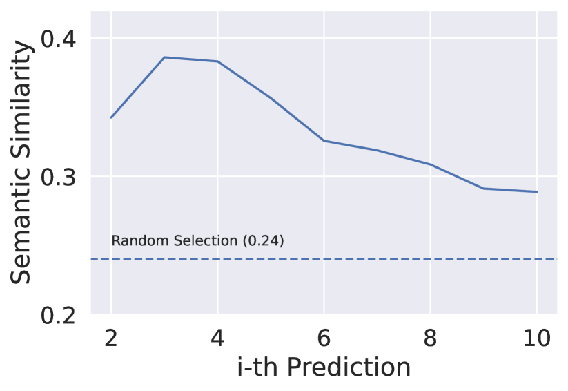
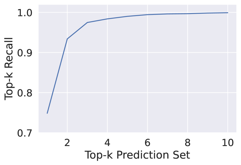
Figure 1: The statistical information of the Top-k prediction sets from a well-trained relation extraction model. (a) shows the average semantic similarity between the ground truth label and its $i$-th prediction. (b) shows the recall of different Top-k prediction set. We can observe that labels existing in the Top-k prediction set has strong connections with the corresponding ground truth label. Besides, the Top-6 prediction set achieves a recall score of more than 0.99, meaning that most ground truth labels exist in Top-6 prediction sets.

We first conduct a pilot experiment to explore whether Top-k prediction sets contain meaningful information. We first train a relation extraction model using RoBERTa-large (Liu et al. 2019) on the TACRED (Zhang et al. 2017) dataset, and then use this well-trained model to obtain the Top-k prediction set of each test sample. The statistical information is visualized in Figure 1. We report the average semantic similarity between the ground truth label and the $i$-th label in the corresponding Top-k prediction set. For each example, we also compute the semantic similarity between its ground truth and a randomly selected relation as the lower bound, denoted as random selection. We find that labels in the Top-k prediction set have strong connections with its ground truth label, while random selection shows much lower similarity. In Figure 1 (b), we show the recall of the Top-k prediction set with different $k$. We can easily observe that the recall grows fast as the $k$ increases, e.g., Top-1 recall is only around 0.75, and Top-6 recall is already larger than 0.99. The above results verify our assumption that the Top-k prediction set contains available information, and we may benefit relation extraction if it can be used properly.

Based on the above observations, we propose Label Graph Network with Top-K Prediction Set (KLG), which could utilize the Top-k prediction set to improve the performance on relation extraction task. We first fine-tune a PLM on downstream datasets with a standard supervised learning paradigm. This PLM then automatically generates the Top-k prediction set for each sample. These Top-k prediction sets will be treated as supplementary information to train KLG. Specifically, KLG first builds a label graph, which sets all pre-defined labels as nodes, and extracts the adjacent information from the Top-k prediction set. In this way, our model could review candidate labels existing in the Top-k prediction set and learn the connections between them.

However, the performance maybe sensitive to a fixed $k$. Performing a grid search is time-expensive and hinders model generalization. Therefore, we considered bypassing the determination of $k$ and letting the model learn by itself from multiple possible Top-k prediction sets (or multiple label graphs). To make the model more robust and learn diverse information from the Top-k prediction set, we design a dynamic $k$-selection mechanism. For a given sample and its Top-k prediction set, we randomly select different Top-$\hat{k}$ predictions to form various label graphs. Then a graph contrastive learning loss is used to guide the representations of the same sample from different graphs to be close (positive examples), while the representations of different samples to be apart from each other (negative examples). Our dynamic $k$-selection mechanism makes KLG more robust and further achieves better performances.

To verify the effectiveness of KLG, we conduct extensive experiments on three different relation extraction datasets. We find that KLG brings significant improvements over strong baseline models and achieves better results than previous state-of-the-art methods (§3.3). Besides, we also explore why does KLG work, and the experiments show that KLG has a strong ability to improve the performance on long-tailed classes (§4.1).

To sum up, our contributions are as follows:

1. We show that labels existing in the Top-k prediction set has strong connections with the corresponding ground truth label, which is largely ignored by previous works.

2. We propose Label Graph Network with Top-K Prediction Set (KLG), which contains a label graph and the dynamic $k$-selection mechanism. KLG could effectively leverage useful information in the Top-k prediction set. We conduct extensive experiments and achieve new state-of-the-art performances on three relation extraction datasets.

3. We also explore why does KLG work and we find that KLG is particularly good at handling long-tailed classes.

2 Our Approach

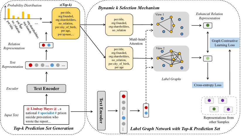
Figure 2: Illustration of our proposed method KLG, the example is taken from TACRED training set. Left: the procedure of Top-k prediction set generation. This is a classical supervised learning paradigm. For each sample, instead of only outputting the label with the highest probability, we extract the Top-k prediction set depending on the probability distribution. Right: the overall architecture of KLG. We first use pre-defined labels and s(Top-k) to build a label graph. Then for each sample, we design a dynamic $k$-selection mechanism to create diverse Top-k prediction sets and label graphs, together with graph contrastive learning. KLG could achieve more powerful relation representations. Better viewed in color.

2.1 Top-k Prediction Set Generation

In the first step, we need to generate the Top-k prediction set for each sample. In this research, we use a pre-trained PLM to train a baseline model $M$ and obtain the Top-k prediction sets. Specifically, for a given input sentence $s$ and two target entities $e_{1}$ and $e_{2}$, we first use an entity marker to inclose the entities, and add the entity type information before each target entity. The above two markers highlight the entities and are demonstrated as crucial for relation extraction. Then we use the max-pooling of the entity spans as the entity representations $\textbf{e}_{1}$ and $\textbf{e}_{2}$, where $\textbf{e}_{1},\textbf{e}_{2}\in\mathbb{R}^{d}$. $d$ is the hidden size of the PLM’s output, e.g., 1024 for the RoBERTa-large model. After concatenating the representations of the head entity and the tail entity, we use a single layer to obtain the relation representation $\textbf{r}\in\mathbb{R}^{d}$.

$$\textbf{r}=MLP([\textbf{e}_{1}||\textbf{e}_{2}]),$$ (1)

where $||$ denotes vector concatenation. Finally, a classification layer with a softmax activation function is used to output the probability distribution of all pre-defined labels.

After we finish the training of baseline model $M$, we use $M$ to predict all samples in the training, dev, and test sets. For each sample, we generate its Top-k prediction set depending on the probability distribution of the classification layer’s output, denoted as s(Top-k).

2.2 Label Graph Fusion

In this subsection, we will fine-tune a new PLM by introducing a label graph to leverage the s(Top-k) effectively. Typically, a graph $\mathcal{G}$ should have a node set $\mathcal{V}$ and an edge set $\mathcal{E}$, denoted as $\mathcal{G(V,E)}$. The edge links a pair of nodes, denoted as the $(u,v)\in\mathcal{E}$, where $u\in\mathcal{V}$ and $v\in\mathcal{V}$, and all the graphs are undirected, i.e., $(u,v)\in\mathcal{E}\leftrightarrow(v,u)\in\mathcal{E}$. The number of nodes is $N=|V|$. For the node representation, we have a feature matrix $\textbf{X}\in\mathbb{R}^{N*d}$, where $d$ is the feature dimension. For convenience, we set this dimension the same as the hidden size of the PLM’s output in §2.1. To represent the edge set $\mathcal{E}$, researchers usually introduce an adjacency matrix $A\in\mathbb{R}^{N*N}$, where $A_{i,j}=1$ if $(u,v)\in\mathcal{E}$ and $A_{i,j}=0$ otherwise.

Suppose the current downstream task has $N$ pre-defined labels, denoted as $c_{1},c_{2},...,c_{N}$. We first initialize the label graph with a feature matrix $\textbf{X}\in\mathbb{R}^{N*d}$, and each node representation $\textbf{h}_{i}$ corresponds to a pre-defined label $c_{i}$. Where X is random initialized and will be optimized during training. Then for each sample, we construct the edge set $\mathcal{E}$ based on its s(Top-k). We set labels in the s(Top-k) are connected, including the self-loop. Specifically, for the node $u$ and node $v$, the edge $(u,v)$ is computed as follows:

$$(u,v)=\begin{cases}1,c_{u},c_{v}\in\textit{s(Top-k)}\\ 0,otherwise,\\ \end{cases}$$ (2)

For a given s(Top-k), the label graph has $\frac{k(k+1)}{2}$ edges. It is worth noticing that if the ground truth label is not in the s(Top-k), then these edges will not link with the ground truth label in the graph. As we can see in Figure 1, there are still very few samples that are not recalled under s(Top-10).

Then we use graph attention network (GAT) (Velickovic et al. 2018) to process the label graph $\mathcal{G}$. A scoring function $e:\mathbb{R}^{d}*\mathbb{R}^{d}\Rightarrow\mathbb{R}$ computes a score for every edge $(u,v)$, where $A_{i,j}=1$. $e(\textbf{h}_{u},\textbf{h}_{v})$ indicates the importance of the features of the neighbor $v$ to the node $u$:

$$e(\textbf{h}_{u},\textbf{h}_{v})=LeakyReLU(a^{T}\cdot[\textit{{W}}\textbf{h}_{u}||\textit{{W}}\textbf{h}_{v}]),$$ (3)

where $a\in\mathbb{R}^{2d{{}^{\prime}}}$m $\textit{{W}}\in\mathbb{R}^{d\times d{{}^{\prime}}}$ are learned parameters, we set $d^{{}^{\prime}}=d$ in this research. After we obtain attention scores across all neighbors of node $u$, a softmax function is used to normalize these scores:

$$\alpha(u,v)=\frac{exp(e(\textbf{h}_{u},\textbf{h}_{v}))}{\sum_{c_{v^{{}^{\prime}}}\in\textit{s(Top-k)}}exp(e(\textbf{h}_{u},\textbf{h}_{v^{{}^{\prime}}}))}$$ (4)

Then we compute a weighted average of transformed features of the neighbor node using the normalized attention coefficient as the new node representation:

$$\textbf{h}^{{}^{\prime}}_{u}=\sigma(\sum_{c_{v}\in\textit{s(Top-k)}}\alpha(u,v)\cdot\textit{{W}}\textbf{h}_{v})$$ (5)

Then we use a mutil-head attention layer (Vaswani et al. 2017) to aggregate the relation representation r and those $k$ node representations $\textbf{X}_{k}$, and r is the query vector:

$$\hat{\textbf{r}}=MultiHeadAtt(\textbf{r},\textbf{X}_{k},\textbf{X}_{k}).$$ (6)

Where $\textbf{X}_{k}$ contains $k$ node representations corresponding to labels in s(Top-k). $\hat{\textbf{r}}$ is the enhanced relation representation that learns label connections from the label graph. Finally, we concatenate the two relation representations and use an MLP layer with a softmax activation function to obtain the final prediction:

$$p=MLP([\textbf{r}||\hat{\textbf{r}}])$$ (7)

We use a standard cross-entropy loss to optimize our model, and the loss is denoted as $\mathcal{L}^{CE}$.

2.3 Dynamic $k$-Selection Mechanism

While leveraging the label graph could achieve consistent improvements, one crucial problem is determining a proper $k$ in s(Top-k). In §2.2, we select the $k$ where the Top-k recall achieves 0.99 on the dev set. However, the performance may sensitive to a fixed $k$ and result in an unstable output. In this subsection, we propose a Dynamic $k$ Selection Mechanism (DS), which could create diverse Top-k prediction sets for each sample, and further leverages graph contrastive learning for better relation representations. To be specific, we first choose the value of $k$ that the Top-$k$ recall achieves 0.99 on the dev set. Then we randomly choose another $k^{{}^{\prime}}$ from the following uniform distribution:

$$k^{{}^{\prime}}\in[\lceil\frac{1}{2}k\rceil,\lceil\frac{3}{2}k\rceil].$$ (8)

Where $\lceil*\rceil$ means round up, and equation 8 ensures that we could select diverse $k$ at each training step.

After applying the dynamic $k$-selection mechanism, we can build multiple label graphs using different Top-k prediction sets. In our research, we use s(Top-k) and s(Top-$k^{{}^{\prime}}$) to construct two different label graphs for a given sample, denoted as $\mathcal{G}$ and $\mathcal{G}^{{}^{\prime}}$. To fully use these label graphs and achieve more powerful relation representations, we design a graph contrastive learning loss. Specifically, for a given sample $x_{i}$, we first compute two relation representations $\hat{\textbf{r}_{i}}$ and $\hat{\textbf{r}_{i}}^{{}^{\prime}}$ through Equation 6. These two relation representations are generated from the specific sample $x_{i}$, thus $\hat{\textbf{r}_{i}}^{{}^{\prime}}$ can be seen as the augmentation version of $\hat{\textbf{r}_{i}}$. We treat $\hat{\textbf{r}_{i}}$ and $\hat{\textbf{r}_{i}}^{{}^{\prime}}$ as a positive pair. Additionally, in a mini-batch, samples that hold the same label with $x_{i}$ also can be seen as positives for $\hat{\textbf{r}_{i}}$, and samples that hold different labels are treated as negative samples. Then for a mini-batch with $N$ training examples, denoted as ${(x_{i},y_{i})}_{i=1}^{N}$, we have $2N$ relation representations, where the last half examples of the batch are the augmented views of the first half, and they share the same labels. And $i\in I=[2N]$ is the index of an arbitrary relation representations. Our graph contrastive learning loss is defined as follows:

$$\mathcal{L}^{GCL}=\sum\limits_{i\in I}\frac{-1}{P(i)}\sum\limits_{j\in P(i)}\mathcal{L}_{i,j}^{GCL}$$ (9)

$$\mathcal{L}_{i,j}^{GCL}=log\frac{exp(\hat{\textbf{r}_{i}}^{T}\cdot\hat{\textbf{r}_{j}}/\tau)}{exp(\hat{\textbf{r}_{i}}^{T}\cdot\hat{\textbf{r}_{j}}/\tau)+\sum\limits_{q\in N(i)}exp(\hat{\textbf{r}_{i}}^{T}\cdot\hat{\textbf{r}_{q}}/\tau)}$$ (10)

Here $P(i)$ is the positive example set for $\hat{\textbf{r}_{i}}$, and $N(i)$ is the negative example set for $\hat{\textbf{r}_{i}}$. $\tau$ is a scalar temperature parameter. Through graph contrastive learning, KLG could effectively utilize diverse label graphs and learn more powerful relation representations.

Finally, the overall training loss for KLG is shown as follows:

$$\mathcal{L}=\alpha\mathcal{L}^{CE}+(1-\alpha)\mathcal{L}^{GCL},$$ (11)

where $\alpha$ is a loss weighting factor.

3 Experiments

3.1 Setting

Dataset and Metrics. We evaluate KLG on TACRED (Zhang et al. 2017), TACRED-Revisit (Alt, Gabryszak, and Hennig 2020), and SemEval2010 (Hendrickx et al. 2010), three commonly used relation extraction datasets. Due to the space limitation, we present detailed information about these datasets in the Appendix LABEL:dataset. Following previous work, we use the Micro-F1 score excluding ’No Relation’ as the metric. Besides, we also report the precision, recall, and Macro-F1 score in our detailed analysis.

Model Details. We use Pytorch (Paszke et al. 2019) and RoBERTa-large as the text encoder for both parts of KLG. The checkpoint can be downloaded here. The batch size is 16, and the optimizer is AdamW (Loshchilov and Hutter 2019) with a 1e-5 learning rate and a warm-up strategy. The maximum training epoch is 10, and the maximum input length is 256. The scalar temperature parameter $\tau$ is 0.05, and the loss weighting factor $\alpha$ is 0.9. We set $k$ as the Top-$k$ recall achieves 0.99 on the dev set. The checkpoint that achieves the best result on the dev set is used for testing. We conduct each experiment three times and report the average result to reduce the randomness. Besides, we also report the performances using different backbone networks. Please refer Appendix LABEL:othermodel for more details.

3.2 Comparison Methods

We compare KLG with state-of-the-art RE systems that represent a diverse array of approaches.

Classification-based Methods. These methods fine-tune PLMs on RE datasets with a standard classification loss. LUKE (Yamada et al. 2020) is a popular model for various information extraction tasks, it is pre-trained with large number of external weakly supervised data. IRE (Zhou and Chen 2021) is a strong model which uses entity type marker and achieves impressive performances. RECENT-SpanBERT (Lyu and Chen 2021) designs multi-task learning for better usage of entity type information.

Sequence-to-sequence Methods. These methods use text generation models such as BART (Lewis et al. 2020) and T5 (Raffel et al. 2020) for RE. REBEL (Cabot and Navigli 2021) leverages a BART-large model and is pre-trained on a huge external corpus for RE. TANL(Paolini et al. 2021) reformulates RE as a translation task by utilizing the powerful T5 model. Since the above two methods do not leverage entity type information in their original settings. To have a fair comparison, we re-implement these methods with official code and add the entity type information. We also directly treat relation names as generation objectives and fine-tune a BART model on RE datasets.

Prompt-based Methods. This line of research uses prompt and treats RE as a cloze-style task. PTR (Han et al. 2021) and KnowPrompt (Chen et al. 2022) use different prompt and answer word engineering for RE. While NLI-DeBERTa (Sainz et al. 2021) reformulates relation extraction as an entailment task.

Besides, we also design several other models for comparison. Base Model is the basic network that used for generating the Top-k prediction set in §2.1. Based on the Base Model, we design two improved methods that utilize the Top-k prediction set in different ways. Base Model(P) adds a Prompt $P$ after the input text, where $P$ is: Choose a relation from s(Top-k) for $e_{1}$ and $e_{2}$. Base Model(LS) uses Label Smoothing (Ioffe and Szegedy 2015) and modifies the one-hot label as the soft label.

3.3 Main Results

Table 1 shows the performances on three RE datasets, and we can have the following observations.

KLG outperforms all previous state-of-the-art methods on three RE datasets, including pushing the TACRED F1-score to 75.6%, TACRED-Revisit F1-score to 84.1%, and SemEval2010 F1-score to 90.5%. Compared with the most popular classification-based methods, KLG shows favorable results without any external dataset usage or additional pre-training stages. Although the newly emerging methods offer desirable performances with larger PLMs, such as T5 and DeBERTa, KLG still suppresses them by a large margin. The above results verify the effectiveness of KLG. By utilizing s(Top-k) via a label graph and the dynamic $k$-selection mechanism, KLG could fully use the available information existing in the Top-k prediction set and achieve better performance.

Although we apply different technologies to utilize the Top-k prediction set, the performances of Base Model(P) and Base Model(LS) are undesirable. Base Model(P) shows that directly injecting the Top-k prediction set into the input text can not achieve better performance as we expected, even with the help of a prompt. We think there are two possible reasons for the above phenomenon: 1) the backbone network can not understand the semantic meaning of relation names, and appending the Top-k prediction set after the input text may confuse the model’s encoder, making the model pays less attention to the original input text. 2) With sufficient training samples, models may learn to select a relation name from the Top-k prediction set directly without considering the original input text. As for Base Model(LS), it obtains slight improvements compared with its corresponding baseline model. Meanwhile, KLG achieves much better performances than the above methods.

We also report the ablation study on two crucial components of KLG: 1) the usage of label graph with Top-k prediction set, and 2) the dynamic $k$-selection mechanism. The results show that both parts bring notable improvements over the Base Model. With the help of the label graph, our model could review candidate labels existing in the top-k prediction set and learn useful information from them. In addition, after being equipped with the dynamic $k$-selection mechanism, KLG learns more powerful relation representations and further improves its performance.

	TACRED	TACRED-Rev	SemEval
Classification-based Methods
LUKE	72.7	80.8	90.1
IRE	74.6	83.2	89.8
RECENT	75.2	83.4	-
Sequence-to-Sequence Methods
BART	72.7	81.5	89.5
REBEL	73.7	-	-
TANL	74.8	-	-
Prompt-based Methods
PTR	72.4	81.4	89.9
KnowPrompt	72.4	82.4	90.2
NLI-DeBERTa	73.9	-	-
Ours
Base Model	74.3	83.1	89.6
Base Model(P)	74.1	82.7	89.1
Base Model(LS)	74.6	83.5	89.9
KLG	75.6(+0.4)	84.1(+0.7)	90.5(+0.3)
KLG w/o DS	75.0	83.6	90.1

Table 1: Micro-F1 score of test sets on three relation extraction datasets. Results are all cited from published papers or re-implemented using official code. For each dataset, underlined indicates previous state-of-the-art, bold indicates the best model performance. Results of our methods are averaged over three random seeds, and the results are statistically significant with $p<0.05$.

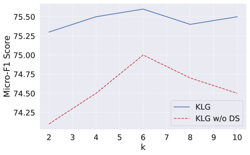
Figure 3: The effectiveness of $k$. We find that the fixed $k$ results in unstable performances. With the help of the dynamic $k$-selection mechanism, KLG could achieve desirable results across a wide range of $k$.

3.4 The Sensitivity of $k$

In this section, we explore the sensitivity of $k$. These results also verify the robustness of our dynamic $k$-selection mechanism (DS). We present the performance on TACRED test set with DS and without DS in Figure 3. We find that without DS, the performances are very sensitive to the $k$-selection, especially when $k$ is too small or too large. With the help of DS, KLG could achieve more stable and much better performances across a wide range of $k$.

4 Analysis

Input Sentence	Ground Truth	Base Model	Top-6 Prediction Set	KLG
PDA’s advisory board includes seven members of congress and …, Thom Hartmann rev. lennox yearwood ….	org:top_members/ employees	org:shareholders	org:shareholders, no_relation, org:top_members/employees, org:founded_by, org:parents, org:subsidiaries	org:top_members/ employees
She testified that she had been forced to sign …, FBI price and wood, under threats of …	per:employee_of	no_relation	no_relation, per:employee_of, per:schools_attended, per:cities_of_residence, per:other_family, per:countries_of_residence	per:employee_of
He was later flown back to Manila, where he reunited with family and friends .	per:cities_of_ residence	per:city_of_birth	per:city_of_birth, no_relation, per:countries_of_residence, per:cities_of_residence, per:city_of_death, per:religion	per:cities_of_ residence

Table 2: Case Study. All examples are extracted from the test set of TACRED. Blue denotes the target entity, and Red denotes the ground truth label existing in the Top-6 prediction set.

4.1 Why Does KLG Work?

		Base Model	KLG
Head Classes (69.6%)	Precision	76.0	78.8(+2.8)
	Recall	79.7	77.3(-2.4)
	Micro-F1	77.8	78.1(+0.3)
Tail Classes (3.6%)	Precision	74.4	75.3(+0.9)
	Recall	69.6	74.7(+5.1)
	Micro-F1	71.9	75.0(+3.1)
All Classes	Micro-F1	74.3	75.6(+1.3)
	Macro-F1	61.2	65.2(+4.0)

Table 3: Performances of TACRED test set on head classes, tail classes, and all classes. To have a clear picture, we report the precision, recall, Micro-F1 score, and Macro-F1 score. After filtering out the ’No Relation’ class, we choose 10 classes with the highest frequency as head classes, and 10 other classes with the lowest frequency are long-tailed classes.

As KLG could learn label connections from the Top-k prediction set and reconsider these labels, which may particularly benefit long-tailed classes. We want to explore why does KLG work from the perspective of long-tailed classes. We report fine-grained experimental results on the test set of TACRED. After filtering out the ’No Relation’ class, we choose 10 classes with the highest frequency as head classes, and 10 other classes with the lowest frequency are long-tailed classes. The proportion of head classes samples is 69.6%, and only 3.6% for long-tailed classes. We report the precision, recall, and Micro-F1 score on both head and long-tailed classes. As the Macro-F1 score is more suitable for the imbalanced scenario, we also report the Macro-F1 score on the whole dataset. We can draw following conclusions from Table 3.

Both models have undesirable performances on the long-tailed classes than on the head classes. This indicates that dealing with long-tailed classes is more challenging. As for the performance gap between these two types of classes, KLG is much smaller than Base Model, i.e., -3.1% v.s. -5.9%. Compared with the Base Model, KLG achieves a remarkable improvement in terms of Macro-F1 score, i.e., 4.0 point absolute improvement. The above results show that KLG is particularly good at handling imbalanced scenario.

Considering the performances of long-tailed classes, the improvement of KLG over the Base Model is more higher on long-tailed classes than on head classes (+3.1% v.s. +0.3%). Furthermore, KLG dramatically improves the recall from 69.6% to 74.7%, with around 5.1 points absolute improvement. We attribute this to the usage of the Top-k prediction set and the dynamic $k$-selection mechanism. As the Top-k prediction set may contain candidate long-tailed classes which are ignored by previous methods, KLG could review these labels and finally benefit the performance of long-tailed classes. These results show that the performance improvements are mainly from the long-tailed classes.

As for the head classes, although the Micro-F1 score has slight improvement, we find that the precision improves over 2.8%, since KLG mitigates the trend of false positive on the head classes by paying more attention to the long-tailed classes. Besides, we also observe the recall of head classes has a significant degradation. One possible reason is that KLG tends to classify head classes as long-tailed classes, resulting in a relatively low recall of head classes.

Figure 4: The norm of the classifier weight vector for each class. The class indexes are sorted by the number of samples (head to tail). We exclude the ’No Relation’ to better view the trend. We can observe that KLG has similar vector norms across all classes.

We also conduct visualization to verify the above conclusion intuitively. Previous works (Kang et al. 2020; Tiong et al. 2021; Peng et al. 2021) show that the $l2$ norm of the classifier weight vector is positively correlated with the number of training samples of the corresponding label. Having a high weight norm for a class means that the classifier tends to output a high logit score for this class, so a good classifier should have essentially the same vector weights. Figure 4 shows the weight norm of the Base Model and KLG. The number of samples is reduced from the left (head classes) to the right (long-tailed classes). We can observe that the weight norms of the Base Model are significantly different for different classes. On the other hand, KLG has a more balanced weight norm compared with the Base Model, thus is more friendly for long-tailed classes and finally achieves remarkable improvements.

4.2 Case Study

To have a clear picture of the effectiveness of KLG, we present several cases in Table 2. From the first and third cases, we can see that although the Base Model outputs the wrong prediction, the prediction is related to the ground truth label. For example, in the first case, the ground truth is org:top_membersemployees, while the label with the highest probability is org:shareholders, which has a similar semantic meaning with org:top_membersemployees. We find the Top-6 prediction set contains the ground truth label, but this information was ignored by previous works. As for the second case, although Base Model gives per:employee_of a high probability, it finally outputs ’no_relation’ as the final prediction. Since the majority of examples in the training set are labeled as ’no_relation’, Base Model tends to output a high logit score for ’no_relation’ class. KLG successfully outputs correct predictions in all examples by reviewing candidate labels and learning useful information from the Top-k prediction set.

5 Related Work

Relation extraction is a well-studied and popular task in natural language processing. Early works leveraged machine learning to tackle relation extraction, and these methods can be divided into two categories: feature-based methods (Kambhatla 2004; Boschee, Weischedel, and Zamanian 2005; Chan and Roth 2010; Sun, Grishman, and Sekine 2011; Nguyen and Grishman 2014) and kernel-based methods (Culotta and Sorensen 2004; Zhou et al. 2007; Giuliano et al. 2007; Qian et al. 2008; Nguyen, Moschitti, and Riccardi 2009; Sun and Han 2014). Feature-based methods heavily rely on handcraft features. These features are domain-specific and data-specific. Kernel-based methods need existing NLP tools to transform an input sentence into a parse tree. However, the NLP tools may make mistakes during processing, which may negatively affect the model’s performance.

Then deep learning methods have been the mainstream solutions for RE. Liu et al. (2013) first adopt deep learning for RE via convolutional neural network. Zeng et al. (2015) proposed a model named Piecewise Convolutional Neural Networks(PCNN). Also, there are lots of works modified convolutional neural network and recurrent neural network for RE (Santos, Xiang, and Zhou 2015; Miwa and Bansal 2016; Zhou et al. 2016; She et al. 2018; He et al. 2018; Su et al. 2017).

Recently, transformer-based methods which leverage PLMs have shown impressive performances on RE (Yamada et al. 2020; Xue et al. 2021; Li et al. 2020, 2021; Roy and Pan 2021; Zhou and Chen 2021; Lyu and Chen 2021). These methods used the PLMs such as BERT and Roberta as backbone network, and designed novel components or multi-task learning framework for better performance.

Prompt-based methods (Radford et al. 2019) were drawn some attention in recent research as well. PTR (Han et al. 2021) and KnowPrompt (Chen et al. 2022) used a human-designed prompt with different label verbalizers for each relation. While NLI-DeBERTa (Sainz et al. 2021) reformulated relation extraction as an entailment task with relation descriptions. Sequence-to-sequence methods are another interesting research direction for RE. REBEL (Cabot and Navigli 2021) focused on joint entity and relation extraction and pre-trained a BART-large model with external datasets. TANL (Paolini et al. 2021) used T5 and backbone network and achieved impressive performance on various information extraction tasks.

In this research, we focus on leveraging the top-k prediction set for RE, which is not explored in past work.

6 Conclusion

In this paper, we first reveal that the Top-k prediction set of a given sample contains helpful information when dealing with relation extraction. Then we propose Label Graph Network with Top-k Prediction Set (KLG), a new model that fully utilizes the Top-k prediction set by building a label graph neural network with the dynamic $k$-selection mechanism. By digging the potentially useful information from the Top-k prediction set and reviewing these labels, KLG achieves new state-of-the-art results on three relation extraction datasets. Besides, KLG is particularly good at handling long-tailed classes. We hope this research could inspire researchers to further effectively explore the usage of the Top-k prediction set.

%nobibliographyaaai23

References

- Alt, Gabryszak, and Hennig (2020) Alt, C.; Gabryszak, A.; and Hennig, L. 2020. TACRED Revisited: A Thorough Evaluation of the TACRED Relation Extraction Task. In Jurafsky, D.; Chai, J.; Schluter, N.; and Tetreault, J. R., eds., ACL 2020, 1558–1569. Association for Computational Linguistics.
- Boschee, Weischedel, and Zamanian (2005) Boschee, E.; Weischedel, R.; and Zamanian, A. 2005. Automatic information extraction. In Proceedings of the International Conference on Intelligence Analysis, volume 71. Citeseer.
- Cabot and Navigli (2021) Cabot, P. H.; and Navigli, R. 2021. REBEL: Relation Extraction By End-to-end Language generation. In Moens, M.; Huang, X.; Specia, L.; and Yih, S. W., eds., Findings of EMNLP 2021, 2370–2381. Association for Computational Linguistics.
- Chan and Roth (2010) Chan, Y. S.; and Roth, D. 2010. Exploiting Background Knowledge for Relation Extraction. In COLING 2010, 152–160.
- Chen et al. (2022) Chen, X.; Zhang, N.; Xie, X.; Deng, S.; Yao, Y.; Tan, C.; Huang, F.; Si, L.; and Chen, H. 2022. KnowPrompt: Knowledge-aware Prompt-tuning with Synergistic Optimization for Relation Extraction. In Laforest, F.; Troncy, R.; Simperl, E.; Agarwal, D.; Gionis, A.; Herman, I.; and Médini, L., eds., WWW 2022, 2778–2788. ACM.
- Culotta and Sorensen (2004) Culotta, A.; and Sorensen, J. S. 2004. Dependency Tree Kernels for Relation Extraction. In Proceedings of the 42nd Annual Meeting of the Association for Computational Linguistics, 21-26 July, 2004, Barcelona, Spain., 423–429.
- Devlin et al. (2019) Devlin, J.; Chang, M.; Lee, K.; and Toutanova, K. 2019. BERT: Pre-training of Deep Bidirectional Transformers for Language Understanding. In Burstein, J.; Doran, C.; and Solorio, T., eds., NAACL-HLT 2019, 4171–4186. Association for Computational Linguistics.
- Giuliano et al. (2007) Giuliano, C.; Lavelli, A.; Pighin, D.; and Romano, L. 2007. FBK-IRST: Kernel methods for semantic relation extraction. In Proceedings of the 4th International Workshop on Semantic Evaluations, 141–144. Association for Computational Linguistics.
- Han et al. (2021) Han, X.; Zhao, W.; Ding, N.; Liu, Z.; and Sun, M. 2021. PTR: Prompt Tuning with Rules for Text Classification. CoRR, abs/2105.11259.
- He et al. (2018) He, Z.; Chen, W.; Li, Z.; Zhang, M.; Zhang, W.; and Zhang, M. 2018. SEE: Syntax-aware entity embedding for neural relation extraction. In Thirty-Second AAAI Conference on Artificial Intelligence.
- Hendrickx et al. (2010) Hendrickx, I.; Kim, S. N.; Kozareva, Z.; Nakov, P.; Séaghdha, D. Ó.; Padó, S.; Pennacchiotti, M.; Romano, L.; and Szpakowicz, S. 2010. SemEval-2010 Task 8: Multi-Way Classification of Semantic Relations between Pairs of Nominals. In SemEval@ACL 2010.
- Ioffe and Szegedy (2015) Ioffe, S.; and Szegedy, C. 2015. Batch Normalization: Accelerating Deep Network Training by Reducing Internal Covariate Shift. In Bach, F. R.; and Blei, D. M., eds., Proceedings of the 32nd International Conference on Machine Learning, ICML 2015, Lille, France, 6-11 July 2015, volume 37 of JMLR Workshop and Conference Proceedings, 448–456. JMLR.org.
- Kambhatla (2004) Kambhatla, N. 2004. Combining lexical, syntactic, and semantic features with maximum entropy models for extracting relations. In Proceedings of the ACL 2004 on Interactive poster and demonstration sessions, 22. Association for Computational Linguistics.
- Kang et al. (2020) Kang, B.; Xie, S.; Rohrbach, M.; Yan, Z.; Gordo, A.; Feng, J.; and Kalantidis, Y. 2020. Decoupling Representation and Classifier for Long-Tailed Recognition. In 8th International Conference on Learning Representations, ICLR 2020, Addis Ababa, Ethiopia, April 26-30, 2020. OpenReview.net.
- Lewis et al. (2020) Lewis, M.; Liu, Y.; Goyal, N.; Ghazvininejad, M.; Mohamed, A.; Levy, O.; Stoyanov, V.; and Zettlemoyer, L. 2020. BART: Denoising Sequence-to-Sequence Pre-training for Natural Language Generation, Translation, and Comprehension. In Proceedings of the 58th Annual Meeting of the Association for Computational Linguistics, 7871–7880. Online: Association for Computational Linguistics.
- Li et al. (2021) Li, B.; Ye, W.; Huang, C.; and Zhang, S. 2021. Multi-view Inference for Relation Extraction with Uncertain Knowledge. In AAAI 2021. AAAI Press.
- Li et al. (2020) Li, B.; Ye, W.; Sheng, Z.; Xie, R.; Xi, X.; and Zhang, S. 2020. Graph Enhanced Dual Attention Network for Document-Level Relation Extraction. In COLING 2020, 1551–1560. International Committee on Computational Linguistics.
- Liu et al. (2013) Liu, C.; Sun, W.; Chao, W.; and Che, W. 2013. Convolution neural network for relation extraction. In International Conference on Advanced Data Mining and Applications, 231–242. Springer.
- Liu et al. (2019) Liu, Y.; Ott, M.; Goyal, N.; Du, J.; Joshi, M.; Chen, D.; Levy, O.; Lewis, M.; Zettlemoyer, L.; and Stoyanov, V. 2019. RoBERTa: A Robustly Optimized BERT Pretraining Approach. CoRR, abs/1907.11692.
- Loshchilov and Hutter (2019) Loshchilov, I.; and Hutter, F. 2019. Decoupled Weight Decay Regularization. In ICLR 2019. OpenReview.net.
- Lyu and Chen (2021) Lyu, S.; and Chen, H. 2021. Relation Classification with Entity Type Restriction. In Zong, C.; Xia, F.; Li, W.; and Navigli, R., eds., Findings of ACL/IJCNLP 2021, volume ACL/IJCNLP 2021 of Findings of ACL, 390–395. Association for Computational Linguistics.
- Miwa and Bansal (2016) Miwa, M.; and Bansal, M. 2016. End-to-end relation extraction using lstms on sequences and tree structures. arXiv preprint arXiv:1601.00770.
- Nguyen and Grishman (2014) Nguyen, T. H.; and Grishman, R. 2014. Employing Word Representations and Regularization for Domain Adaptation of Relation Extraction. In ACL 2014, 68–74.
- Nguyen, Moschitti, and Riccardi (2009) Nguyen, T. T.; Moschitti, A.; and Riccardi, G. 2009. Convolution Kernels on Constituent, Dependency and Sequential Structures for Relation Extraction. In EMNLP 2009, 1378–1387.
- Paolini et al. (2021) Paolini, G.; Athiwaratkun, B.; Krone, J.; Ma, J.; Achille, A.; Anubhai, R.; dos Santos, C. N.; Xiang, B.; and Soatto, S. 2021. Structured Prediction as Translation between Augmented Natural Languages. In ICLR 2021. OpenReview.net.
- Paszke et al. (2019) Paszke, A.; Gross, S.; Massa, F.; Lerer, A.; Bradbury, J.; Chanan, G.; Killeen, T.; Lin, Z.; Gimelshein, N.; Antiga, L.; Desmaison, A.; Köpf, A.; Yang, E. Z.; DeVito, Z.; Raison, M.; Tejani, A.; Chilamkurthy, S.; Steiner, B.; Fang, L.; Bai, J.; and Chintala, S. 2019. PyTorch: An Imperative Style, High-Performance Deep Learning Library. In NeurIPS 2019, 8024–8035.
- Peng et al. (2021) Peng, Z.; Huang, W.; Guo, Z.; Zhang, X.; Jiao, J.; and Ye, Q. 2021. Long-tailed Distribution Adaptation. In Shen, H. T.; Zhuang, Y.; Smith, J. R.; Yang, Y.; Cesar, P.; Metze, F.; and Prabhakaran, B., eds., MM ’21: ACM Multimedia Conference, Virtual Event, China, October 20 - 24, 2021, 3275–3282. ACM.
- Qian et al. (2008) Qian, L.; Zhou, G.; Kong, F.; Zhu, Q.; and Qian, P. 2008. Exploiting constituent dependencies for tree kernel-based semantic relation extraction. In Proceedings of the 22nd International Conference on Computational Linguistics-Volume 1, 697–704. Association for Computational Linguistics.
- Radford et al. (2019) Radford, A.; Wu, J.; Child, R.; Luan, D.; Amodei, D.; Sutskever, I.; et al. 2019. Language models are unsupervised multitask learners. OpenAI blog, 1(8): 9.
- Raffel et al. (2020) Raffel, C.; Shazeer, N.; Roberts, A.; Lee, K.; Narang, S.; Matena, M.; Zhou, Y.; Li, W.; and Liu, P. J. 2020. Exploring the Limits of Transfer Learning with a Unified Text-to-Text Transformer. J. Mach. Learn. Res., 21: 140:1–140:67.
- Reimers and Gurevych (2019) Reimers, N.; and Gurevych, I. 2019. Sentence-BERT: Sentence Embeddings using Siamese BERT-Networks. In Inui, K.; Jiang, J.; Ng, V.; and Wan, X., eds., EMNLP-IJCNLP 2019, 3980–3990. Association for Computational Linguistics.
- Roy and Pan (2021) Roy, A.; and Pan, S. 2021. Incorporating medical knowledge in BERT for clinical relation extraction. In Moens, M.; Huang, X.; Specia, L.; and Yih, S. W., eds., EMNLP 2021, 5357–5366. Association for Computational Linguistics.
- Sainz et al. (2021) Sainz, O.; de Lacalle, O. L.; Labaka, G.; Barrena, A.; and Agirre, E. 2021. Label Verbalization and Entailment for Effective Zero and Few-Shot Relation Extraction. In Moens, M.; Huang, X.; Specia, L.; and Yih, S. W., eds., EMNLP 2021, 1199–1212. Association for Computational Linguistics.
- Santos, Xiang, and Zhou (2015) Santos, C. N. d.; Xiang, B.; and Zhou, B. 2015. Classifying relations by ranking with convolutional neural networks. arXiv preprint arXiv:1504.06580.
- She et al. (2018) She, H.; Wu, B.; Wang, B.; and Chi, R. 2018. Distant Supervision for Relation Extraction with Hierarchical Attention and Entity Descriptions. In IJCNN 2018, 1–8. IEEE.
- Soares et al. (2019) Soares, L. B.; FitzGerald, N.; Ling, J.; and Kwiatkowski, T. 2019. Matching the Blanks: Distributional Similarity for Relation Learning. In ACL 2019.
- Su et al. (2017) Su, Y.; Liu, H.; Yavuz, S.; Gur, I.; Sun, H.; and Yan, X. 2017. Global relation embedding for relation extraction. arXiv preprint arXiv:1704.05958.
- Sun, Grishman, and Sekine (2011) Sun, A.; Grishman, R.; and Sekine, S. 2011. Semi-supervised Relation Extraction with Large-scale Word Clustering. In The 49th Annual Meeting of the Association for Computational Linguistics: Human Language Technologies, Proceedings of the Conference, 19-24 June, 2011, Portland, Oregon, USA, 521–529.
- Sun and Han (2014) Sun, L.; and Han, X. 2014. A Feature-Enriched Tree Kernel for Relation Extraction. In ACL 2014, 61–67.
- Tiong et al. (2021) Tiong, A. M. H.; Li, J.; Lin, G.; Li, B.; Xiong, C.; and Hoi, S. C. H. 2021. Improving Tail-Class Representation with Centroid Contrastive Learning. CoRR, abs/2110.10048.
- Vaswani et al. (2017) Vaswani, A.; Shazeer, N.; Parmar, N.; Uszkoreit, J.; Jones, L.; Gomez, A. N.; Kaiser, L.; and Polosukhin, I. 2017. Attention is All you Need. In Guyon, I.; von Luxburg, U.; Bengio, S.; Wallach, H. M.; Fergus, R.; Vishwanathan, S. V. N.; and Garnett, R., eds., Advances in Neural Information Processing Systems 30: Annual Conference on Neural Information Processing Systems 2017, December 4-9, 2017, Long Beach, CA, USA, 5998–6008.
- Velickovic et al. (2018) Velickovic, P.; Cucurull, G.; Casanova, A.; Romero, A.; Liò, P.; and Bengio, Y. 2018. Graph Attention Networks. In ICLR 2018. OpenReview.net.
- Xue et al. (2021) Xue, F.; Sun, A.; Zhang, H.; and Chng, E. S. 2021. GDPNet: Refining Latent Multi-View Graph for Relation Extraction. In AAAI 2021, 14194–14202. AAAI Press.
- Yamada et al. (2020) Yamada, I.; Asai, A.; Shindo, H.; Takeda, H.; and Matsumoto, Y. 2020. LUKE: Deep Contextualized Entity Representations with Entity-aware Self-attention. In EMNLP 2020.
- Ye et al. (2019) Ye, W.; Li, B.; Xie, R.; Sheng, Z.; Chen, L.; and Zhang, S. 2019. Exploiting Entity BIO Tag Embeddings and Multi-task Learning for Relation Extraction with Imbalanced Data. In Korhonen, A.; Traum, D. R.; and Màrquez, L., eds., ACL 2019. Association for Computational Linguistics.
- Zeng et al. (2015) Zeng, D.; Liu, K.; Chen, Y.; and Zhao, J. 2015. Distant supervision for relation extraction via piecewise convolutional neural networks. In Proceedings of the 2015 Conference on Empirical Methods in Natural Language Processing, 1753–1762.
- Zhang et al. (2017) Zhang, Y.; Zhong, V.; Chen, D.; Angeli, G.; and Manning, C. D. 2017. Position-aware Attention and Supervised Data Improve Slot Filling. In EMNLP 2017.
- Zhou et al. (2007) Zhou, G.; Zhang, M.; Ji, D.; and Zhu, Q. 2007. Tree kernel-based relation extraction with context-sensitive structured parse tree information. In Proceedings of the 2007 Joint Conference on Empirical Methods in Natural Language Processing and Computational Natural Language Learning (EMNLP-CoNLL).
- Zhou et al. (2016) Zhou, P.; Shi, W.; Tian, J.; Qi, Z.; Li, B.; Hao, H.; and Xu, B. 2016. Attention-based bidirectional long short-term memory networks for relation classification. In Proceedings of the 54th Annual Meeting of the Association for Computational Linguistics (Volume 2: Short Papers), volume 2, 207–212.
- Zhou and Chen (2021) Zhou, W.; and Chen, M. 2021. An Improved Baseline for Sentence-level Relation Extraction. CoRR, abs/2102.01373.