Practical Exposure Correction: Great Truths Are Always Simple

Abstract

Improving the visual quality of the given degraded observation by correcting exposure level is a fundamental task in the computer vision community. Existing works commonly lack adaptability towards unknown scenes because of the data-driven patterns (deep networks) and limited regularization (traditional optimization), and they usually need time-consuming inference. These two points heavily limit their practicability. In this paper, we establish a Practical Exposure Corrector (PEC) that assembles the characteristics of efficiency and performance. To be concrete, we rethink the exposure correction to provide a linear solution with exposure-sensitive compensation. Around generating the compensation, we introduce an exposure adversarial function as the key engine to fully extract valuable information from the observation. By applying the defined function, we construct a segmented shrinkage iterative scheme to generate the desired compensation. Its shrinkage nature supplies powerful support for algorithmic stability and robustness. Extensive experimental evaluations fully reveal the superiority of our proposed PEC. The code is available at https://rsliu.tech/PEC.

(a) Comparing running time	(b) Visual comparisons with deep networks	(c) Visual comparisons with traditional methods

Figure 1: Practicability evaluation. In (a), we compare nine advanced deep networks and nine traditional methods (please refer to the experimental part for detailed sources) by using different computational resources. In (b), we demonstrate a group of visual comparisons among two deep networks and PEC on the same scene [3] but with different exposure conditions (the left top and right bottom are overexposure and underexposure, respectively). In (c), we show visual comparisons among two traditional methods and PEC on different scenes [9, 24] with different degrees of underexposure. Obviously, our PEC realizes the best visual effects and spends least running time simultaneously, which fully indicates the practicability of PEC.

1 Introduction

With the demand for high-quality image resources with correct exposure in various areas, the imaging capability (e.g., photosensitivity, aperture size) of terminal devices has become increasingly important. However, only focusing on improving the device level will still be difficult to overcome imaging challenges in severe scenarios, e.g., back-light, non-uniform illumination, etc. The exposure correction techniques [7, 22, 1, 11, 13] emerges as the times require. There have designed copious advanced approaches to handle this task in the past few decades, they will be introduced in the upcoming subsection. Moreover, we describe our contributions at the end of this section.

1.1 Related Work

Generally, exposure correction contains two typical scenes, i.e., under and overexposure. The former has attracted more attention than the latter from interests, so the former developed faster. Recently, a few works proposed a unified model to handle these two cases simultaneously.

The mainstream solutions of underexposure correction contain traditional optimization and data-driven learning. Traditional optimization [6, 2, 8, 17, 10] focuses on designing regularization to constrain the desired objectives, which are derived from the Retinex theory [14]. LIME [8] was a well-known work, and utilized the form presented in RTV [34] to estimate the illumination. As mentioned in this work, existing schemes were mostly hard to provide appropriate exposure in challenging scenes. Learning a deep model is the current mainstream manner for correcting underexposure images. Specifically, most of them [37, 38, 31] lay emphasis on devising the network architecture to provide an effective mapping toward reference goals. Considering the limitation on learning specific distributions, more and more works [7, 19, 22] constructed unsupervised learning strategies to satisfy the requirements in various scenarios. Unfortunately, there are still limitations in these works. Such as, the difficulty in designing the effective training losses.

Very recently, researchers has began to design deep architectures [1, 11] for addressing underexposure and overexposure correction at the same time. The work in [1] defined a multi-scale coarse-to-fine processing pipeline and constructed a new dataset with a broad range of exposure levels. Huang et al., designed a series of exposure correction deep networks from different perspectives [11, 12, 13], e.g., spatial-frequency interaction. However, these existing works for general exposure correction commonly adopted the supervised methods which made them excessively dependent on training data, leading to poor generalization.

1.2 Our Contributions

To overcome the above issues, we create a new algorithm to perform exposure correction effectively and efficiently in diversified adverse imaging conditions as far as possible. As shown in Fig. Practical Exposure Correction: Great Truths Are Always Simple, we can observe the practicability of PEC, i.e., realizing the best visual effects on different challenging scenes with the fastest inference speed. Our main contributions can be concluded as

• By rethinking the task goal of exposure correction, we establish a practical and general exposure correction solution with exposure-sensitive compensation. It adopts a simple linear operator according to different cases, i.e., applying addition in underexposure and performing subtraction for overexposure.

• An exposure adversarial function is developed to fully exploit latent structural information from the observation itself for capturing the compensation. It not only conquers the poor generalization from the data-driven learning paradigm but also avoids the complex inference from traditional optimization.

• Through applying the exposure adversarial function, we build the segmented shrinkage iterative scheme to generate the compensation that is desired in our established general algorithm. This approach only requires few manually-adjusted parameters, and its shrinkage property ensures the stability of PEC.

• The evaluations on multiple challenging datasets fully verify the superiority of our PEC. A prominent point is that the inference speed of PEC on different platforms is significantly faster than other methods. For example, it just costs 0.0009s to process a 2K image on the device with GeForce RTX 2080Ti GPU.

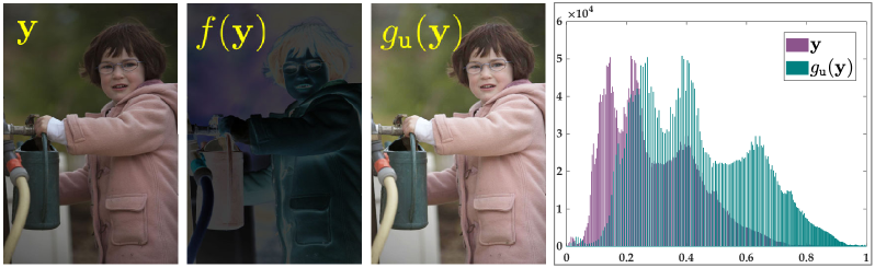
(a) Underexposure image correction ($c=1$)

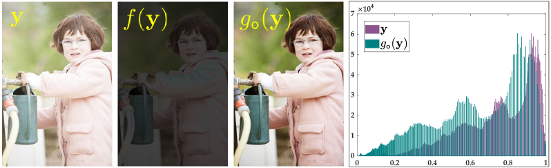
(b) Overexposure image correction ($c=-1$)

Figure 2: Effects of the warm start. The left three columns demonstrate the visual results of each component in the warm start, and the last column plots the histogram comparisons among results before and after correction. It can be observed that the corrected outputs almost keep the same distribution in trend as the inputs.

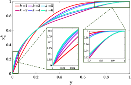
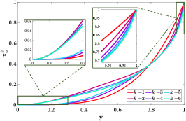
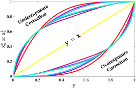
Figure 3: The iterative processes of $h_{\mathtt{u}}^{k}(\mathbf{y})$ and $h_{\mathtt{o}}^{k}(\mathbf{y})$ in the first built-in block, where $\mathbf{y}\in[0,1]^{1\times M}$ is a vector, and the total iterative numbers $K=6$.

2 Rethinking Exposure Correction

Generally, underexposure image correction aims at enlarging small pixel values in some underexposed areas make them visible, while overexposure image correction focuses on narrowing the large pixel values to make them appear. From this plain opinion, a straightforward direction is to add a map into the underexposure observation to achieve the effect of magnification. Similarly, we can delete a map from the overexposure observation to acquire the shrinking normal image.

Based on the above finding, we define the following formula to clearly describe exposure correction.

$$\left\{\begin{aligned} &\mathbf{x}_{\mathtt{u}}=\mathbf{y}+\bm{\epsilon}(\mathbf{y}),\mathrm{if}\;\mathbf{y}\in\mathbb{U},\\ &\mathbf{x}_{\mathtt{o}}=\mathbf{y}-\bm{\epsilon}(\mathbf{y}),\mathrm{if}\;\mathbf{y}\in\mathbb{O},\\ \end{aligned}\right.$$ (1)

where $\mathbf{y}$, $\mathbf{x}_{\mathtt{u}}$ and $\mathbf{x}_{\mathtt{o}}$ denote the observation with incorrect exposure, the underexposure corrected output and the overexposure corrected output, respectively. The sets $\mathbb{U}$ and $\mathbb{O}$ represent the underexposure image domain and overexposure image domain, respectively. The function $\bm{\epsilon}(\mathbf{y})$ is our defined exposure-sensitive compensation which is closely related to the given observation.

In this way, we clearly point out the critical component of the exposure correction task, then focus on estimating the exposure-sensitive compensation while correcting exposure. Next, we will introduce how to design an effective algorithm for acquiring it.

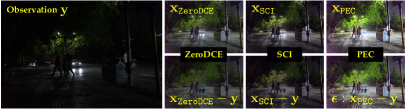
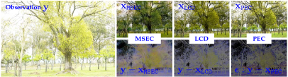
Figure 4: Comparing the derived compensations among different methods in underexposure (left) and overexposure (right) cases. Here we compare two representative underexposure correction methods, i.e., ZeroDCE [7] and SCI [22], and two recent overexposure correction methods, i.e., MSEC [1] and LCD [28].

3 Methodology

In this section, we will introduce exposure adversarial function, warm start with compensation, and segmented shrinkage iterative scheme.

3.1 Exposure Adversarial Function

Existing works [1, 11] have proved that applying massive data to the meticulously-designed network is indeed an effective way to learn the mapping $\bm{\epsilon}$. However, a common symptom for learning-based works is inevitable, i.e., unstable outcomes toward unseen scenarios. In other words, this scheme just fits specific distribution but ignores task modeling for exposure correction in essence. To provide a general computational mode, as for the given variable $\mathbf{z}\in[0,1]^{m\times n}$ (either underexposed or overexposed), we define the exposure adversarial function as

$$f(\mathbf{z})=c\mathbf{z}\otimes(\mathbf{1}-\mathbf{z}),\\$$ (2)

where $\otimes$ represents the element-wise multiplication, $0\leq c\leq 1$ is a coefficient for controlling exposure level.

Lemma 3.1.

The exposure adversarial function as presented in Eq. (2), it satisfies the axisymmetric property on x-axis, i.e., $f(\mathbf{1-z})=f(\mathbf{z})$.

The above-built function combines the input ($\mathbf{z}$) and reversed input ($\mathbf{1-z}$) to generate the result with a closed-form range, i.e., $f(\mathbf{z})\in[0,c]^{m\times n}$. Actually, $\mathbf{z}$ and $\mathbf{1-z}$ keep a relationship of checks and balances, and this is why we call “adversarial”. More importantly, when facing different observations with exposure levels, this function can consistently output a stable solution in view of the axisymmetric property presented in Lemma 3.1.

We would like to explain that this exposure adversarial function is a core support for constructing the exposure-sensitive compensation $\bm{\epsilon}$ presented in Eq. (1). More detail will be introduced in the following.

3.2 Warm Start with Compensation

We first construct a warm start with compensation to provide an effective initialization, which can be formulated as

$$\left\{\begin{aligned} &g_{\mathtt{u}}(\mathbf{y})=\mathbf{y}+f(\mathbf{y}),\;\;\mathrm{if}\,\mathtt{UC},\\ &g_{\mathtt{o}}(\mathbf{y})=\mathbf{y}-f(\mathbf{y}),\;\;\mathrm{if}\,\mathtt{OC},\\ \end{aligned}\right.$$ (3)

where $g_{\mathtt{u}}$ and $g_{\mathtt{o}}$ are the corrected outputs for underexposure and overexposure cases, respectively.

Algorithm 1 Practical Underexposure Correction

0:  The underexposure observation $\mathbf{y}$, the iteration numbers $T$ and $K^{1},...,K^{T}$, the coefficient $c$.

1:  $g_{\mathtt{u}}(\mathbf{y})=\mathbf{y}+f(\mathbf{y})$,

2:  for $t\leq T$ do

3:     for $k\leq K^{t}$ do

4:        $\mathbf{x}_{\mathtt{u}}^{k}=g_{\mathtt{u}}(\mathbf{y})+f(\mathbf{x}_{\mathtt{u}}^{k-1})$,

5:     end for

6:     $g_{\mathtt{u}}(\mathbf{y})=\mathbf{x}_{\mathtt{u}}^{K^{t}}$.

7:  end for

8:  return  The corrected output $\mathbf{x}_{\mathtt{u}}^{K^{T}}$.

Fig. 2 explores the effects of our warm start operation. We can easily observe that the warm start ameliorates the exposure of the input correctly. From the histogram distribution, it is worth noting that the corrected outputs do not destroy the intrinsic distribution of the observation, i.e., the original pixel-level correspondences in the observation are still reserved. In addition, this experiment also manifests that we can only use the warm start to correct exposure in some simple cases.

Lemma 3.2.

If the exposure level is consistent, i.e., $c$ is identical on different exposure scenes, the warm start processes between different exposure cases satisfy the symmetric property, that is $g_{\mathtt{u}}(\mathbf{1-y})=1-g_{\mathtt{o}}(\mathbf{y})$.

We know that underexposure images generally contain lots of pixels with small values which are even close to zero. Similarly, overexposure images always have lots of pixels with significant values which are nearly equal to one. From this appearance, there possibly exists a mutual connection of forward and reverse between underexposure and overexposure correction. As presented in Lemma 3.2, our warm start built above satisfies the symmetric property among different exposure cases, which also indicates the rationally of our constructing process.

Compared to the task modeling in Eq. (1), in the warm start process, the desired exposure-sensitive compensation $\bm{\epsilon}$ is exactly equal to $f$, i.e., $\bm{\epsilon}(\mathbf{y})=f(\mathbf{y})$.

Metrics		KinD (IJCV ’21)	ZeroDCE (CVPR ’20)	MSEC (CVPR ’21)	RUAS (CVPR ’21)	UTVNet (ICCV ’21)	LCD (ECCV ’22)	FEC (ECCV ’22)	URetinex (CVPR ’22)	SCI (CVPR ’22)	PEC
Underexposure	PSNR$\uparrow$	15.6897	14.8025	20.7083	13.8939	18.5640	22.6598	22.9983	13.4200	20.5109	18.4411
	SSIM$\uparrow$	0.6845	0.6047	0.7758	0.1943	0.5893	0.8113	0.8203	0.6378	0.7129	0.7382
	LPIPS$\downarrow$	0.2478	0.2668	0.1808	0.2745	0.2533	0.1471	0.1782	0.2537	0.1843	0.1841
	DE$\uparrow$	7.0382	6.7807	7.4151	6.7804	7.1458	7.4114	7.3600	6.9806	7.3594	7.4450
	LOE$\downarrow$	377.69	350.96	260.45	496.93	227.48	120.03	147.49	417.99	95.65	22.29
	NIQE$\downarrow$	2.8416	3.3212	2.9387	3.1368	4.2256	2.9458	3.0721	2.7346	2.6997	2.6843
Overexposure	PSNR$\uparrow$	9.7730	8.5916	19.3523	4.8380	13.5211	22.2832	22.8995	8.5030	6.9746	19.1298
	SSIM$\uparrow$	0.5856	0.4764	0.7674	0.1943	0.2907	0.8235	0.8253	0.5106	0.3612	0.7803
	LPIPS$\downarrow$	0.2945	0.3405	0.1834	0.7410	0.4923	0.1341	0.1609	0.3611	0.5055	0.1677
	DE$\uparrow$	6.9735	6.7789	7.5965	2.1515	6.6062	7.4810	7.4671	6.8123	6.1999	7.6040
	LOE$\downarrow$	102.57	338.90	354.95	1663.92	762.05	195.01	257.92	389.22	231.17	9.10
	NIQE$\downarrow$	2.6464	2.7607	2.6890	6.5999	5.0407	2.6631	2.9606	2.6201	2.6709	2.5588

Table 1: Quantitative comparisons on the Exposure-Errors dataset [1]. Three full-reference metrics (i.e., PSNR, SSIM and LPIPS), and three no-reference metrics (DE, LOE, and NIQE) are reported.

3.3 Segmented Shrinkage Iterative Scheme

We have achieved an acceptable corrected quality shown in Fig. 2, more common and challenging scenes need to be researched still. By combining the exposure adversarial function and the solution presented in Eq. (1), we define a segmented shrinkage iterative scheme that is composed of the shrinkage built-in block. And each built-in block belongs to an iterative process, whose basic iterative step is

$$\left\{\begin{aligned} &h_{\mathtt{u}}^{k}(\mathbf{y}):\mathbf{x}_{\mathtt{u}}^{k}=g_{\mathtt{u}}(\mathbf{y})+f(\mathbf{x}_{\mathtt{u}}^{k-1}),\\ &h_{\mathtt{o}}^{k}(\mathbf{y}):\mathbf{x}_{\mathtt{o}}^{k}=g_{\mathtt{o}}(\mathbf{y})-f(\mathbf{x}_{\mathtt{o}}^{k-1}),\\ \end{aligned}\right.$$ (4)

where $1\leq k\leq K^{t}$ represents the iterative number in $t$-th ($1\leq t\leq T$, $1\leq T\leq 3$) shrinkage built-in block. When $k=1$, we define $\mathbf{x}_{\mathtt{u}}^{0}=\mathbf{x}_{\mathtt{u}}^{{K}^{t}},\mathbf{x}_{\mathtt{o}}^{0}=\mathbf{x}_{\mathtt{o}}^{{K}^{t}}$. As for the first block (i.e., $t=1$), we set $\mathbf{x}_{\mathtt{u}}^{0}=g_{\mathtt{u}}(\mathbf{y}),\mathbf{x}_{\mathtt{o}}^{0}=g_{\mathtt{o}}(\mathbf{y})$.

Theorem 3.1.

With the Lemma 3.1 and Lemma 3.2, there exists the symmetric property between underexposure and overexposure cases in each iterative step upon given built-in block, i.e., $h_{\mathtt{u}}^{k}(\mathbf{1-y})=\mathbf{1}-h_{\mathtt{o}}^{k}(\mathbf{y})$.

Input (Full Size)	KinD	ZeroDCE	MSEC	RUAS	UTVNet
LCD	FEC	URetinex	SCI	PEC	PEC (Full Size)

Figure 5: Visual comparisons on the Exposure-Errors dataset [1].

[b] Resolution & Platform KinD ZeroDCE MSEC^$\dagger$ RUAS UTVNet^$\ddagger$ LCD FEC URetinex SCI PEC 1280$\times$720 CPU 2.3844 17.7944 0.3007 2.8807 8.6610 4.1292 4.8920 8.9093 0.0823 0.0269 GPU 2.1340 0.0013 0.2349 0.0309 0.3837 1.6064 0.0132 0.2348 0.0007 0.0003 1920$\times$1080 CPU 5.1322 40.4684 0.4899 4.8915 13.4690 8.2461 12.1834 23.3995 0.1550 0.0515 GPU 4.6483 0.0014 0.4730 0.0463 - 2.8085 0.0143 0.4876 0.0009 0.0006 2560$\times$1440 CPU 8.0632 69.7165 0.9081 5.6561 22.5862 14.7200 23.0975 33.4536 0.2702 0.0927 GPU 7.9920 0.0016 0.8838 0.0821 - 4.7721 0.0164 0.8318 0.0020 0.0009

• The running platform of this work is different from other methods, we evaluated it on a PC with a NIVIDIA TITAN Xp GPU.

• This work requires too much video memory on the high-resolution images, leading to a failure in producing results.

Table 2: Comparing running time (second) on the samples with different resolutions from the Exposure-Errors dataset. The running time is computed on a PC with Geforce RTX 2080Ti GPU and Intel Xeon W-2135 Processor.

Datasets	Metrics	SRIE	NPEA	WVM	JIEP	LIME	RRM	LR3M	STAR	SDD	PEC
MEF	DE$\uparrow$	6.9282	7.0714	6.9436	7.0119	7.3263	7.0530	6.9869	6.9377	7.0835	7.0390
	LOE$\downarrow$	261.70	422.32	210.26	469.86	802.33	311.39	359.26	59.33	436.54	30.76
	NIQE$\downarrow$	4.6592	3.5469	3.4742	3.4314	3.7662	3.9385	4.4172	3.5251	4.3136	3.0053
	TIME (S)$\downarrow$	0.4301	5.4156	0.2310	1.7648	0.1899	11.5471	169.4971	0.5434	3.3234	0.0080
LIME	DE$\uparrow$	6.8967	6.8963	6.8516	6.8924	7.5492	6.9878	6.8873	6.7729	7.0355	7.0752
	LOE$\downarrow$	212.61	436.45	140.12	226.84	621.42	283.46	297.97	51.39	309.93	76.63
	NIQE$\downarrow$	4.9814	5.2273	4.0273	3.9927	4.1357	4.2415	4.4396	4.4369	4.5146	3.8963
	TIME (S)$\downarrow$	1.0270	15.9399	0.8995	5.2193	0.2915	28.3221	76.7941	0.9033	6.9280	0.0247

Table 3: Numerical scores among different methods on the MEF and LIME datasets. We evaluated the CPU running time on a PC with an Intel Core i7-8700K Processor.

Input	SRIE	NPEA	WVM	JIEP	LIME	STAR	SDD	PEC

Figure 6: Visual comparisons on the LIME dataset. From the second to last column, we plot the zoomed-in regions and the corresponding difference map with the original input in the gray-scale space. The HSV colormap is applied to highlight.

Furthermore, we can conclude Theorem 3.1 from the properties (see Lemma 3.1 and Lemma 3.2) presented in above two subsections. It builds an explicit connection between underexposure and overexposure correction for each basic iterative step. As shown in Fig. 3, we also plot the corrected process over the given vector $\mathbf{y}$ which belongs to $[0,1]$. A distinct appearance is that the curve presents a shrinkage status along with the iteration increase. Besides, we can see that Theorem 3.1 can be easily proved from a geometry view. We can make a conclusion that, our constructed segmented shrinkage iterative scheme still keeps the inherent relationship among different tasks of exposure correction. It actually provides an implicit constraint to narrow down the solution space for ensuring stability.

Finally, as for each iterative step in the underexposure case, we have $\bm{\epsilon}(\mathbf{y})=f(\mathbf{y})+f(\mathbf{x}_{\mathtt{u}}^{k-1})$, where $\mathbf{x}_{\mathtt{u}}^{k-1}$ is related to $\mathbf{y}$. Because of the nested iteration, here we do not provide a general final form for the compensation. Alg. 1 presents our computational flow for underexposure case, the overexposure case just need change the symbol “$+$” to “$-$”.

3.4 Discussion

As presented above, the exposure-sensitive compensation is the essential component that appeared in each part of the algorithmic main body. Here we investigate its effects from the visualization. As shown in Fig. 4, we can easily see that for the underexposure case, our PEC can automatically recognize the overexposure regions to avoid further strengthening (e.g., the car light). As for the overexposure case, the overall structure and details of our generated compensation are closer to the original observation.

By performing the same derived process of compensation, the compensations of other compared methods can be acquired. These constructed compensations actually produce similar content to ours. But as shown in the right subfigure, limited to the data-specific learning pattern, the undesired artifacts are introduced in the MSEC to blur the structural information (see the bottom row for MSEC). In a word, this experiment fully proves that our solution for exposure correction is traceable and effective enough.

Input	LIME	SDD	ZeroDCE	MSEC	RUAS	LCD	FEC	SCI	PEC

Figure 7: Visual comparisons on different challenging scenes. From the first to last row, the observations are respectively sampled from UFDD [24], ExDARK [20], LSRW [9], and DARKFACE [35] datasets. More results can be found in the Supplemental Materials.

4 Experimental Results

4.1 Comparisons with Advanced Networks

There were nine advanced deep networks being compared, including six underexposure correction methods (i.e., KinD [37], ZeroDCE [7], RUAS [19], UTVNet [38], URetinex [31], and SCI [22]), and three exposure correction approaches (i.e., MSEC [1], LCD [28], FEC [12]). We randomly sampled 500 images from the Exposure-Errors testing dataset [1] with the settings of relative EVs -1.5 and +1.5 to evaluated the performance of underexposure and overexposure, respectively. As for evaluated metrics, we adopted three full-reference metrics (i.e., PSNR, SSIM, and LPIPS [36]), and three no-reference metrics (i.e., DE [27], LOE [29], NIQE [23]).

	Dark Face Detector			Enhancer + Detector (Finetune)
Method	HLA	REG	MAET	LIME	ZeroDCE	MSEC	RUAS	LCD	FEC	SCI	PEC
mAP	0.607	0.514	0.526	0.644	0.665	0.659	0.642	0.654	0.603	0.663	0.677
	Nighttime Semantic Segmentator			Enhancer + Segmentator (Finetune)
Method	DANNet	CIC	GPS-GLASS	LIME	ZeroDCE	MSEC	RUAS	LCD	FEC	SCI	PEC
mIoU	0.398	0.264	0.380	0.397	0.399	0.377	0.363	0.381	0.375	0.393	0.416

Table 4: Performance comparisons on other vision tasks. We retrain the detector/segmentator in all cases containing the enhancer.

Quantitative Evaluation. Table 1 reported quantitative results among different methods on the Exposure-Errors dataset. It should be noticed that the top 3 methods on full-reference metrics (i.e., MSEC, LCD, FEC) all adopted the Exposure-Errors training dataset to acquire their models on all exposure cases so their full-reference scores were significant. It can be easily observed that our PEC performs best on the no-reference metrics and gets competitive scores on full-reference metrics for both underexposure and overexposure datasets. In a word, our results are more close to natural image distribution from the statistical perspective.

Qualitative Evaluation. Fig. 5 demonstrated visual comparisons. PEC provides prominent visual effects for both two cases, especially in structural depict and exposure control. It’s worth emphasizing that the results of methods trained with Exposure-Errors datasets (e.g. MSEC, LCD and FEC) are unstable, especially appearing in unexpected artifacts and color distortion.

Comparing Running Time. As shown in Table 2, we take three cases with different resolutions into account, including 1280$\times$720, 1920$\times$1080, and 2560$\times$1440. To provide a comprehensive evaluation, we reported running times on the CPU and GPU for different cases, respectively. Obviously, our method was faster enough than all the advanced networks. As for the resolution of the 2560$\times$1440, our method just needs 0.0009s, which was equal to 1111 FPS for a video with 2K resolution, and it surpassed far away the frame rate in the human eyes.

4.2 Comparisons with Traditional Schemes

Because our proposed PEC belongs to a non-learning paradigm, it is essential to evaluate its performance by comparing it with traditional schemes. The compared methods including NPEA [29], SRIE [5], WVM [6], JIEP [2], LIME [8], RRM [17], LR3M [25], STAR [33], SDD [10]. We tested the performance on two small-scale no-reference datasets LIME [8] (10 images) and MEF [21] (17 images). Three no-reference metrics that appeared in the previous subsection were utilized to evaluate the quantitative scores.

As reported in Table 3, our PEC performed competitive results. It is worth noting that PEC spends the least running time, which are 100 times faster than the second method LIME (a representative work). Fig. 6 demonstrates visual comparisons. We also plotted the difference with original input. In contrast, PEC avoids introducing some unknown artifacts in the sky, but enhances the foreground effectively.

4.3 Exploring Scene Adaptability

To fully evaluate the scene adaptability, we consider challenging examples from different real-world datasets. Here we compare two representative traditional schemes (i.e., LIME and SDD), three unsupervised networks (i.e., ZeroDCE, RUAS, and SCI), and three supervised networks (i.e., MSEC, LCD, and FEC) whose models can address both underexposure and overexposure correction.

As for underexposure correction, we demonstrate visual comparisons of different challenging scenes in Fig. 7. It can be obviously seen that our proposed PEC perform significantly for all scenes. It is because our method does not need any pre-training process, which ensured a general adaptation. Additionally, PEC fully exploited the observation inherent information to realize correction, without introducing any additionally formulated priors to satisfy the specific scene assumptions. Further, Fig. 8 evaluate the results of overexposure case. Since most of methods above are designed for underexposure cases, here we just compared PEC with MSEC, LCD, and FEC. Obviously, all compared methods appeared unknown artifacts and color distortion with different levels. While our PEC wins the best performer, especially in the case of appropriate correction for some possible originally overexposed regions.

Input	MSEC	LCD	FEC	PEC

Figure 8: More visual comparisons of overexposure correction. As for the top two rows, the observations are acquired from SICE [3] and UFDD [24], respectively. The observations in bottom two rows come from the free stock photo website Pexel. More results can be found in the Supplemental Materials.

Input	SCI	MSEC	PEC	Label	Input	ZeroDCE	DANNet	PEC	Label
(a) Dark Face Detection					(b) Nighttime Semantic Segmentation

Figure 9: Visual comparisons on other vision tasks.

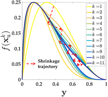
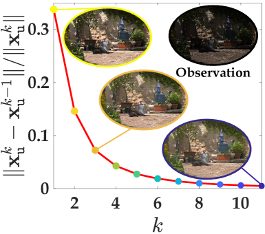
(a) Toy: $f(\mathbf{x}_{\mathtt{u}}^{k})$ v.s. $\mathbf{y}$	(b) Practical: $\frac{\|\mathbf{x}_{\mathtt{u}}^{k}-\mathbf{x}_{\mathtt{u}}^{k-1}\|}{\|\mathbf{x}_{\mathtt{u}}^{k}\|}$ v.s. $k$

Figure 10: The convergence behaviors of PEC. The left plotted the convergence behavior in a toy example (where the observation $\mathbf{y}\in[0,1]^{1\times M}$). The right plotted curve of relative errors and intermediate results, where the underexposed observation $\mathbf{y}\in\mathbb{U}$ is showed in the right top corner of (b).

4.4 Other Vision Applications

Here we adopted the DARKFACE [35] and ACDC [26] datasets for evaluating detection and segmentation respectively, and we followed the data partition as presented in [22]. To ensure a better adaptation, we finetuned all the vision models on the corrected outputs. The number of epochs for detection and segmentation was set to 10 and 30, respectively. We adopted SGD optimizer for these two tasks, the momentum, weight decay, and learning rate were set as {0.9, 3$\times 10^{-4}$, 5$\times 10^{-4}$} and {0.9, 5$\times 10^{-4}$, 2.5$\times 10^{-4}$} for detection and segmentation, respectively.

To fully evaluate the performance, we not only compared a part of the correction methods, but also considered specific methods for detection (including HLA [30], REG [18], and MAET [4]) and segmentation (including DANNet [32], CIC [16], GPS-GLASS [15]). As demonstrated in Table 4 and Fig. 9, our method realizes the best performance quantitatively and qualitatively. This experiment verifies our practicability for downstream vision tasks.

5 Algorithmic Analyses

In this section, we investiged the convergence behavior and parameter analyses of PEC.

5.1 Convergence Behavior Analysis

Here we further explored the convergence behaviors from the toy and practical examples. As shown in Fig. 10, the phenomenon of presenting shrinkage trajectory in the toy examples reflected the convergent nature of PEC. Moreover, from relative error curve and intermediate results as shown in subfifigure (b), it’s apparent that the corrected results keep the stable exposure consistently and the local textures as well ass details are progressively highlighted with the iteration increasing. In a word, we can argue that our PEC indeed possesses the excellent convergence property. In addition, we found that the corrected result in the 3-rd iteration was almost satisfying. So we empirically define the $1\leq K\leq 3$ in our all experiments.

5.2 Parameters Analysis

In our designed algorithm (see Alg. 1), there exist three groups of parameters that need to be manually defined, i.e., the iteration numbers $T,K$, and the exposure control coefficient $c$. The previous subsection has proved that the structural information is progressively compensated along with the iteration $k$ increase.. As shown in Fig. 11, we explored the effects of $T$ and $c$ for corrected output. Subfigure (a) demonstrates the mapping in the range of a given underexposed observation. Subfigure (b) showed the corrected results among cases of cases appearing in (a). It can be easily observed that $T$ and $c$ all decided on the exposure level, and the $T$ had more sensible brightening effects than the coefficient $c$. Moreover, we set $c=1$ for most underexposed scenes, but as for the overexposed cases, we set $c<1$ because of the overexposed levels are not extreme enough.

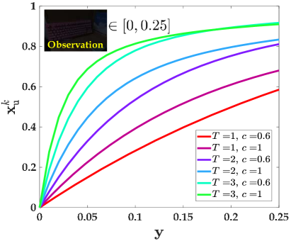
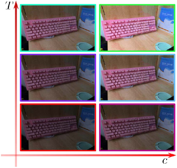
(a) Curves of different settings	(b) Outputs for cases in (a)

Figure 11: Parameters analysis of iteration $T$ and coefficient $c$.

6 Concluding Remarks

This work developed a novel, practical, and general exposure correction algorithm which successfully aggregates the advantages of significant computational efficiency and visual-friendly image quality. PEC also possesses excellent algorithmic properties in stability and convergence. Abundant evaluations were performed to show our superiority.

Broader Impacts. PEC actually provides a new perspective for addressing the task of exposure correction. Benefiting from the representation of the task’s intrinsic demand and beneficial information extracted from observation, it only requires some simple linear operators (addition/subtraction and multiplication) to generate the desired corrected outputs. With the advantages of real-time processing and no introduction of any non-linear operations, PEC can be easily embedded into hardware chips (e.g., FPGA) to service the actual demand. Besides, compared with existing methods, much fewer parameters need to be manually adjusted. In fact, these parameters can be acquired by a learning manner to endow more powerful capability of PEC for catering to different task goals (e.g., tracking).

References

- [1] Mahmoud Afifi, Konstantinos G Derpanis, Bjorn Ommer, and Michael S Brown. Learning multi-scale photo exposure correction. In Proceedings of the IEEE/CVF Conference on Computer Vision and Pattern Recognition, pages 9157–9167, 2021.
- [2] Bolun Cai, Xianming Xu, Kailing Guo, Kui Jia, Bin Hu, and Dacheng Tao. A joint intrinsic-extrinsic prior model for retinex. In Proceedings of the IEEE/CVF International Conference on Computer Vision, 2017.
- [3] Jianrui Cai, Shuhang Gu, and Lei Zhang. Learning a deep single image contrast enhancer from multi-exposure images. IEEE Transactions on Image Processing, PP(99):1–1, 2018.
- [4] Ziteng Cui, Guo-Jun Qi, Lin Gu, Shaodi You, Zenghui Zhang, and Tatsuya Harada. Multitask aet with orthogonal tangent regularity for dark object detection. In Proceedings of the IEEE/CVF International Conference on Computer Vision, pages 2553–2562, 2021.
- [5] Xueyang Fu, Yinghao Liao, Delu Zeng, Yue Huang, Xiao-Ping Zhang, and Xinghao Ding. A probabilistic method for image enhancement with simultaneous illumination and reflectance estimation. IEEE Transactions on Image Processing, 24(12):4965–4977, 2015.
- [6] Xueyang Fu, Delu Zeng, Yue Huang, Xiao-Ping Zhang, and Xinghao Ding. A weighted variational model for simultaneous reflectance and illumination estimation. In Proceedings of the IEEE/CVF Conference on Computer Vision and Pattern Recognition, 2016.
- [7] Chunle Guo, Chongyi Li, Jichang Guo, Chen Change Loy, Junhui Hou, Sam Kwong, and Runmin Cong. Zero-reference deep curve estimation for low-light image enhancement. In Proceedings of the IEEE/CVF Conference on Computer Vision and Pattern Recognition, pages 1780–1789, 2020.
- [8] Xiaojie Guo, Yu Li, and Haibin Ling. Lime: Low-light image enhancement via illumination map estimation. IEEE Transactions on Image Processing, 26(2):982–993, 2017.
- [9] Jiang Hai, Zhu Xuan, Ren Yang, Yutong Hao, Fengzhu Zou, Fang Lin, and Songchen Han. R2rnet: Low-light image enhancement via real-low to real-normal network. arXiv preprint arXiv:2106.14501, 2021.
- [10] Shijie Hao, Xu Han, Yanrong Guo, Xin Xu, and Meng Wang. Low-light image enhancement with semi-decoupled decomposition. IEEE transactions on multimedia, 22(12):3025–3038, 2020.
- [11] Jie Huang, Yajing Liu, Xueyang Fu, Man Zhou, Yang Wang, Feng Zhao, and Zhiwei Xiong. Exposure normalization and compensation for multiple-exposure correction. In Proceedings of the IEEE/CVF Conference on Computer Vision and Pattern Recognition, pages 6043–6052, 2022.
- [12] Jie Huang, Yajing Liu, Feng Zhao, Keyu Yan, Jinghao Zhang, Yukun Huang, Man Zhou, and Zhiwei Xiong. Deep fourier-based exposure correction network with spatial-frequency interaction. In European Conference on Computer Vision, 2022.
- [13] Jie Huang, Man Zhou, Yajing Liu, Mingde Yao, Feng Zhao, and Zhiwei Xiong. Exposure-consistency representation learning for exposure correction. In Proceedings of the 30th ACM International Conference on Multimedia, pages 6309–6317, 2022.
- [14] Edwin H Land and John J McCann. Lightness and retinex theory. Journal of the Optical Society of America, 1971.
- [15] Hongjae Lee, Changwoo Han, and Seung-Won Jung. Gps-glass: Learning nighttime semantic segmentation using daytime video and gps data. arXiv preprint arXiv:2207.13297, 2022.
- [16] Attila Lengyel, Sourav Garg, Michael Milford, and Jan C van Gemert. Zero-shot day-night domain adaptation with a physics prior. In Proceedings of the IEEE/CVF International Conference on Computer Vision, pages 4399–4409, 2021.
- [17] Mading Li, Jiaying Liu, Wenhan Yang, Xiaoyan Sun, and Zongming Guo. Structure-revealing low-light image enhancement via robust retinex model. IEEE Transactions on Image Processing, 27(6):2828–2841, 2018.
- [18] Jinxiu Liang, Jingwen Wang, Yuhui Quan, Tianyi Chen, Jiaying Liu, Haibin Ling, and Yong Xu. Recurrent exposure generation for low-light face detection. IEEE Transactions on Multimedia, 24:1609–1621, 2021.
- [19] Risheng Liu, Long Ma, Jiaao Zhang, Xin Fan, and Zhongxuan Luo. Retinex-inspired unrolling with cooperative prior architecture search for low-light image enhancement. In Proceedings of the IEEE/CVF Conference on Computer Vision and Pattern Recognition, pages 10561–10570, 2021.
- [20] Yuen Peng Loh and Chee Seng Chan. Getting to know low-light images with the exclusively dark dataset. Computer Vision and Image Understanding, 178:30–42, 2019.
- [21] Kede Ma, Kai Zeng, and Zhou Wang. Perceptual quality assessment for multi-exposure image fusion. IEEE Transactions on Image Processing, 24(11):3345–3356, 2015.
- [22] Long Ma, Tengyu Ma, Risheng Liu, Xin Fan, and Zhongxuan Luo. Toward fast, flexible, and robust low-light image enhancement. In Proceedings of the IEEE/CVF Conference on Computer Vision and Pattern Recognition, pages 5637–5646, 2022.
- [23] Anish Mittal, Rajiv Soundararajan, and Alan C Bovik. Making a ”completely blind” image quality analyzer. IEEE Signal Processing Letters, 20(3):209–212, 2012.
- [24] Hajime Nada, Vishwanath A Sindagi, He Zhang, and Vishal M Patel. Pushing the limits of unconstrained face detection: a challenge dataset and baseline results. In IEEE International Conference on Biometrics Theory, Applications and Systems. IEEE, 2018.
- [25] Xutong Ren, Wenhan Yang, Wen-Huang Cheng, and Jiaying Liu. Lr3m: Robust low-light enhancement via low-rank regularized retinex model. IEEE Transactions on Image Processing, 29:5862–5876, 2020.
- [26] Christos Sakaridis, Dengxin Dai, and Luc Van Gool. Acdc: The adverse conditions dataset with correspondences for semantic driving scene understanding. In Proceedings of the IEEE/CVF International Conference on Computer Vision, pages 10765–10775, 2021.
- [27] Claude E Shannon. A mathematical theory of communication. The Bell system technical journal, 27(3):379–423, 1948.
- [28] Haoyuan Wang, Ke Xu, and Rynson WH Lau. Local color distributions prior for image enhancement. In European Conference on Computer Vision, pages 343–359, 2022.
- [29] Shuhang Wang, Jin Zheng, Hai-Miao Hu, and Bo Li. Naturalness preserved enhancement algorithm for non-uniform illumination images. IEEE Transactions on Image Processing, 22(9):3538–3548, 2013.
- [30] Wenjing Wang, Xinhao Wang, Wenhan Yang, and Jiaying Liu. Unsupervised face detection in the dark. IEEE Transactions on Pattern Analysis and Machine Intelligence, 2022.
- [31] Wenhui Wu, Jian Weng, Pingping Zhang, Xu Wang, Wenhan Yang, and Jianmin Jiang. Uretinex-net: Retinex-based deep unfolding network for low-light image enhancement. In Proceedings of the IEEE/CVF Conference on Computer Vision and Pattern Recognition, pages 5901–5910, 2022.
- [32] Xinyi Wu, Zhenyao Wu, Lili Ju, and Song Wang. A one-stage domain adaptation network with image alignment for unsupervised nighttime semantic segmentation. IEEE Transactions on Pattern Analysis and Machine Intelligence, 2021.
- [33] Jun Xu, Yingkun Hou, Dongwei Ren, Li Liu, Fan Zhu, Mengyang Yu, Haoqian Wang, and Ling Shao. Star: A structure and texture aware retinex model. IEEE Transactions on Image Processing, 29:5022–5037, 2020.
- [34] Li Xu, Qiong Yan, Yang Xia, and Jiaya Jia. Structure extraction from texture via relative total variation. ACM Transactions on Graphics, 2012.
- [35] Wenhan Yang, Ye Yuan, Wenqi Ren, Jiaying Liu, Walter J Scheirer, Zhangyang Wang, Taiheng Zhang, Qiaoyong Zhong, Di Xie, Shiliang Pu, et al. Advancing image understanding in poor visibility environments: A collective benchmark study. IEEE Transactions on Image Processing, 29:5737–5752, 2020.
- [36] Richard Zhang, Phillip Isola, Alexei A Efros, Eli Shechtman, and Oliver Wang. The unreasonable effectiveness of deep features as a perceptual metric. In Proceedings of the IEEE Conference on Computer Vision and Pattern Recognition, pages 586–595, 2018.
- [37] Yonghua Zhang, Jiawan Zhang, and Xiaojie Guo. Kindling the darkness: A practical low-light image enhancer. In ACM Multimedia, 2019.
- [38] Chuanjun Zheng, Daming Shi, and Wentian Shi. Adaptive unfolding total variation network for low-light image enhancement. In Proceedings of the IEEE/CVF International Conference on Computer Vision, pages 4439–4448, 2021.