Absolute frequency measurement of a Yb optical clock at the limit of the Cs fountain

Abstract

We present the new absolute frequency measurement of ytterbium (¹⁷¹Yb) obtained at INRiM with the optical lattice clock IT-Yb1 against the cryogenic caesium (¹³³Cs) fountain IT-CsF2, evaluated through a measurement campaign lasted 14 months. Measurements are performed by either using a hydrogen maser as a transfer oscillator or by synthesizing a low-noise microwave for Cs interrogation using an optical frequency comb. The frequency of the ¹⁷¹Yb unperturbed clock transition ¹S${}_{0}\rightarrow{{}^{3}}$P₀ results to be $518\,295\,836\,590\,863.44(14)\text{\,}\mathrm{H}\mathrm{z}$, with a total fractional uncertainty of $2.7\text{\times}{10}^{-16}$ that is limited by the uncertainty of IT-CsF2. Our measurement is in agreement with the Yb frequency recommended by the Consultative Committee for Time and Frequency (CCTF). This result confirms the reliability of Yb as a secondary representation of the second and is relevant to the process of redefining the second in the International System of Units (SI) on an optical transition.

Keywords : frequency metrology, optical lattice clock, Cs fountain, SI second

1 Introduction

The definition of the SI second is currently realized through a Cs frequency transition in the microwave regime [1, 4, 5, 6, 7, 8, 9, 10, 11, 2, 3]. Nevertheless, in recent years it has been widely demonstrated that optical clocks represent a better frequency standard [12, 13, 14, 15], both in terms of fractional frequency instability and estimated systematic uncertainty. Specific optical transitions are currently indicated by the Consultative Committee for Time and Frequency (CCTF) as secondary representations of the SI second, and recent progress in the field of optical clocks paves the way to a redefinition of the SI second [16, 17, 18]. In 2022, the CCTF published a roadmap stating relevant milestones to be achieved to proceed to a redefinition of the SI second, among which emerge multiple and independent measurements of optical clocks relative to independent Cs primary clocks. One of the secondary representations of the second recommended by the CCTF is the transition ¹S${}_{0}\rightarrow^{3}$P₀ of ¹⁷¹Yb. Absolute frequency measurements of this clock transition have been realized by several metrological institutes worldwide [14, 20, 21, 22, 23, 24, 25, 26, 27, 19]. At INRiM we measured the absolute frequency of the ¹⁷¹Yb clock (IT-Yb1) relative to our local cryogenic Cs fountain (IT-CsF2) [28] and via International Atomic Time (TAI) [29]. Moreover, we measured the frequency ratio between ¹⁷¹Yb and ⁸⁷Sr clock with a transportable optical Sr clock developed at PTB [30], and via VLBI (Very Long Baseline Interferometry) in collaboration with NICT INAF and BIPM [31]. Recently we used the new fiber link between INRiM and SYRTE to measure the Yb clock frequency against the french Cs-Rb fountain [19]

In this article, we report the improvements of our optical lattice clock IT-Yb1 and the results obtained from a new measurement of the Yb absolute frequency against IT-CsF2 over a period of 14 months. The frequency measurement is performed with two different techniques: with the first method, the hydrogen maser is used as a transfer oscillator between the optical clock and the fountain, while with the second method the microwave interrogating the fountain is directly obtained by photonic synthesis on a frequency comb, using the Yb clock laser as a local oscillator.

This paper is organized as follows: in section 2 we describe the main components of our experimental setup, i.e. the Yb clock, the Cs fountain and the two measurement techniques. In section 3 we report the results obtained in terms of Yb absolute frequency. Finally, section 4 presents the conclusions of our work.

2 Experimental setup

2.1 IT-Yb1 and IT-CsF2

IT-Yb1 is the optical lattice clock based on ¹⁷¹Yb atoms developed at INRiM. The uncertainty budget of IT-Yb1 during this measurement campaign is reported in Table 1 and the total relative uncertainty is $1.9\text{\times}{10}^{-17}$. The typical instability of IT-Yb1 is $$2\text{\times}{10}^{-15}$/\sqrt{\tau/$\mathrm{s}$}$. IT-Yb1 is among the optical clocks that regularly submit data to the International Bureau of Weights and Measures (BIPM) for the calibration of the International Atomic Time (TAI) [29, 27, 32, 25, 33].

Table 1: Uncertainty budget Yb optical lattice clock at INRiM. Other shifts are AOM switching, fibre links, and line pulling.

Effect	Rel. Shift/${10}^{-17}$	Rel. Unc./${10}^{-17}$
Density shift	-0.5	0.2
Lattice shift	0.8	1.2
Zeeman shift	-3.12	0.02
Blackbody radiation shift (room)	-234.9	1.2
Blackbody radiation shift (oven)	-1.3	0.6
Static Stark shift	-1.7	0.2
Probe light shift	0.04	0.03
Background gas shift	-0.5	0.2
Servo error	0.0	0.3
Other shifts	0.0	0.1
Grav. redshift	2599.5	0.3
Total	2358.3	1.9

IT-Yb1 and its details have been described in previous work [28, 29]. An ultrastable laser at $1156\text{\,}\mathrm{n}\mathrm{m}$ is frequency duplicated to generate the $578\text{\,}\mathrm{n}\mathrm{m}$ light that is kept resonant with the ¹⁷¹Yb clock transition ¹S${}_{0}\rightarrow^{3}$P₀. A new ultrastable cavity directly stabilizes the $1156\text{\,}\mathrm{n}\mathrm{m}$ radiation instead of its second harmonic at $578\text{\,}\mathrm{n}\mathrm{m}$. It is a horizontal 10-cm-long cavity, made in ultra-low-expansion glass and fused silica mirror, characterized by a flicker floor of $\sim$ $1\text{\times}{10}^{-15}$. Compared to previous publications we improved the evaluation of the lattice shift and the static stark shift. In particular, we changed the optical setup from a horizontal to a vertical optical lattice with the advantage of having the strong axis of the trap contrasting the gravity. In this way, we managed to reduce the minimum trapping depth to 75 $E_{\text{r}}$, where $E_{\text{r}}\simeq h\times 2$ kHz is the recoil energy for Yb and $h$ is the Plank constant. We also decreased the depth of our working point from 200 $E_{\text{r}}$ [28] to 100 $E_{\text{r}}$, with consequent advantages in terms of uncertainty budget. The working point of the lattice frequency is chosen at $\nu_{lattice}=$394\,798\,267\text{\,}\mathrm{M}\mathrm{H}\mathrm{z}$$, and it is continuously measured by an optical comb. Moreover, atoms are loaded into the lattice directly at the working depth $U$, making the atomic temperature of the trapped atoms linear as a function of the lattice depth. It is then possible to apply the approach described in [34, 35] and calculate the relative lattice shift by following the model: $\frac{\delta\nu}{\nu}=-\alpha U-\beta U^{2}$, where $\alpha$ and $\beta$ are two parameters that have to be measured in the specific experimental conditions. We estimate a model uncertainty of $1\text{\times}{10}^{-17}$ [34] resulting from deviation from linearity between the atomic temperature and the lattice depth.

We note that, since the density shift is smaller for lower lattice depth [36], at the new working point of 100 $E_{\text{r}}$ the density shift is reduced by a factor of 10 if compared to previous work [29]. Furthermore, the atomic tunnelling between adjacent lattice sites is suppressed in a vertical lattice [37, 14], making this source of uncertainty negligible.

Eight electrodes are placed on the vertical windows, four on the top window and four on the bottom, to evaluate the static stark shift. By applying voltages of up to $\pm$$150\text{\,}\mathrm{V}$ independently to each electrode, it is possible to measure its contribution along the three spatial directions [38, 39]. With this new setup, we detect a stray electric field of about 1-2 V/cm on the horizontal plane, which is found to change slightly from day to day. The direction of the field suggests that the oven used to generate the Yb atomic beam emits some ionized particles that accumulate on the windows. We manage to compensate for the stray electric field by using the same electrodes. The electric field in the 3 directions is measured typically 3 times per week. As each measurement is independent, we allow the resulting shift to be averaged over the campaign. The resulting shift for the period considered in this work is reported in Table 1.

IT-CsF2 is a cryogenic Cs fountain [10] and since 2013 it operates as a primary frequency standard contributing to the realization of UTC(IT) and TAI, with over 50 TAI calibration campaigns performed and published on the BIPM circular T. The uncertainty budget of IT-CsF2 is reported in Table 2 and the total relative uncertainty is $2.3\text{\times}{10}^{-16}$.

The density shift is evaluated by alternating clock measurements with 2 different atom numbers and extrapolating to zero-density. Indeed, the knowledge of the collisional-shift parameter for performing the extrapolation progressively improves with time, as its computation takes advantage of using historical and newly accumulated data, until some parameter characterizing the shift does change, requiring a new measurement run to re-calibrate the density-shift extrapolation.

In its usual configuration, the local oscillator for this clock is a BVA quartz phase-locked to an H-maser and upconverted to $9.2\text{\,}\mathrm{G}\mathrm{H}\mathrm{z}$ using cascaded multiplication stages and a Dielectric Resonator Oscillator (DRO) [10]. This signal is tuned to the atomic resonance using a Direct Digital Synthesizer (DDS) at about $7.4\text{\,}\mathrm{M}\mathrm{H}\mathrm{z}$, adjusted at each interrogation cycle. The typical short-term stability of IT-CsF2 results from a combination of the Dick effect due to the BVA quartz noise and the atomic background noise due to hot Cs atoms. It ranges between $$2.4\text{\times}{10}^{-13}$/\sqrt{\tau/$\mathrm{s}$}$ in high density regime and $$2.8\text{\times}{10}^{-13}$/\sqrt{\tau/$\mathrm{s}$}$ at low density.

Table 2: Uncertainty budget of IT-CsF2.

Effect	Rel. Shift/${10}^{-16}$	Rel. Unc./${10}^{-16}$
Zeeman shift	1080.3	0.8
Blackbody radiation	-1.45	0.12
Gravitational redshift	260.4	0.1
Microwave leakage	-1.2	1.4
DCP (Distributed Cavity Phase)	-	0.2
Second order cavity pulling	-	0.3
Background gas	-	0.5
Density shift	-19.8	1.6
Total	1318.2	2.3

2.2 The measurement chain

Figure 1 shows the block diagram of the two measurement chains used to compare IT-Yb1 and IT-CsF2.

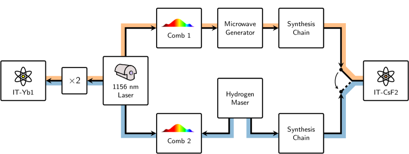
Figure 1: Experimental setup scheme of IT-Yb1 absolute frequency measurement against a IT-CsF2 clock. In blue is represented the path of the H-maser chain, which is our usual measurement chain. In orange instead is shown the microwave-to-optical chain: a new measurement technique we tested in this campaign.

The usual measurement scheme is represented in the lower branch (blue path, hereafter referenced to as "H-maser chain"). Radiation at $1156\text{\,}\mathrm{n}\mathrm{m}$, frequency-stabilised to the ultrastable cavity, is doubled to $578\text{\,}\mathrm{n}\mathrm{m}$ for interrogating the ¹⁷¹Yb clock transition. Part of it is also beaten to a fibre frequency comb stabilised to the same BVA quartz/H-maser system that serves as a local oscillator for IT-CsF2. The IT-Yb1/IT-CsF2 ratio can thus be computed using the comb and H-maser as transfer oscillators. Some of the measurements are instead collected using the measurement chain shown in Fig. 1 with the orange path (hereafter referred to as "Optical Microwave chain"). In this configuration, the frequency comb is referenced to the ultrastable $1156\text{\,}\mathrm{n}\mathrm{m}$ radiation and operates as a low-noise microwave generator to synthesize a signal resonant with the Cs clock transition. The coherent spectral transfer between optical and microwave frequencies is obtained by tightly phase-locking the comb to the optical reference (bandwidth $\approx$ $300\text{\,}\mathrm{k}\mathrm{H}\mathrm{z}$), following a scheme similar to the one described in [40]. The comb pulse train is collected by a fast photodiode, where the 40th harmonic of the repetition rate at $10\text{\,}\mathrm{G}\mathrm{H}\mathrm{z}$ is selected and amplified. We note that coherent transfer of spectral properties of an optical oscillator to a microwave could alternatively be designed for optimized robustness, without recurring to a fast optical comb lock [41] as we did. The noise of the generated microwave is dominated by a flicker phase process at the level of $-105\text{\,}\mathrm{d}\mathrm{B}\mathrm{c}\mathrm{/}\mathrm{H}\mathrm{z}$ at $1\text{\,}\mathrm{H}\mathrm{z}$, limited by detection and signal conditioning stages. The Cs interrogation signal is synthesized from the $10\text{\,}\mathrm{G}\mathrm{H}\mathrm{z}$ input by a two-stage down-conversion. In the first stage, we produce a $9.2\text{\,}\mathrm{G}\mathrm{H}\mathrm{z}$ microwave by mixing to a $800\text{\,}\mathrm{M}\mathrm{H}\mathrm{z}$ radio-frequency obtained by downscaling the input $10\text{\,}\mathrm{G}\mathrm{H}\mathrm{z}$ signal. This is then brought to resonance with the Cs transition by mixing to a DDS at about $7.4\text{\,}\mathrm{M}\mathrm{H}\mathrm{z}$, adjusted at each clock cycle. The flicker phase noise contributed by this chain is $-106\text{\,}\mathrm{d}\mathrm{B}\mathrm{c}\mathrm{/}\mathrm{H}\mathrm{z}$ at $1\text{\,}\mathrm{H}\mathrm{z}$ Fourier frequency, corresponding to an instability of $4\text{\times}{10}^{-16}\text{\,}$ at $1\text{\,}\mathrm{s}$, with a temperature sensitivity of $0.07\text{\,}\mathrm{p}\mathrm{s}\mathrm{/}\mathrm{K}$. The ultrastable $1156\text{\,}\mathrm{n}\mathrm{m}$ laser that is used as a seed for the microwave synthesis is also calibrated by IT-Yb1 during the clock operation.

3 Results

3.1 Absolute frequency measurement of Yb

As usual with atomic clocks, data is processed and reported as fractional frequencies $y=r/r_{0}-1$, where $r$ is the frequency measurement and $r_{0}$ is an arbitrary reference frequency. For this analysis, the reference is chosen consistent with the recommended value of the secondary representation of the second for the Yb transition, i.e. $518\,295\,836\,590\,863.63\text{\,}\mathrm{H}\mathrm{z}$, which has an uncertainty of $1.9\text{\times}{10}^{-16}$ as established by CCTF in 2021 [42]. The use of fractional frequency linearizes equations and is convenient for computations with numbers with many digits [43, 44, 16].

(

a)

(

Figure 2: a) Fractional frequency ratio of IT-Yb1 and IT-CsF2 reported as $y$ (see main text). Data were collected from June 2021 to September 2022 using the H-maser chain (blue dots) and the Optical Microwave chain (orange dots). b) Same data averaged monthly. The grey line represents the average fractional frequency ratio and the shaded area its uncertainty.

b)

We collected data from June 2021 to September 2022. Within this period, we have collected a total of 32 days of data with common uptime between IT-Yb1 and IT-CsF2 using the H-maser chain and a total of 6.9 days of data using the Optical Microwave chain. Data from the combs and IT-Yb1 are collected with a sampling time of $1\text{\,}\mathrm{s}$. Data from IT-CsF2, either the frequency measurement relative to the maser or the optically generated microwave, are recorded with a sampling time of $864\text{\,}\mathrm{s}$. Data from the optical clock and optical combs are averaged in bins with a duration of $864\text{\,}\mathrm{s}$ and combined with the Cs fountain data. The recorded data collected in these $864\text{\,}\mathrm{s}$ bins is shown in Fig. 2a, while Fig. 2b shows the same data averaged monthly. The shaded area represents the average fractional frequency ratios over the entire campaign and its uncertainty. All uncertainties include the systematic uncertainties of the clocks.

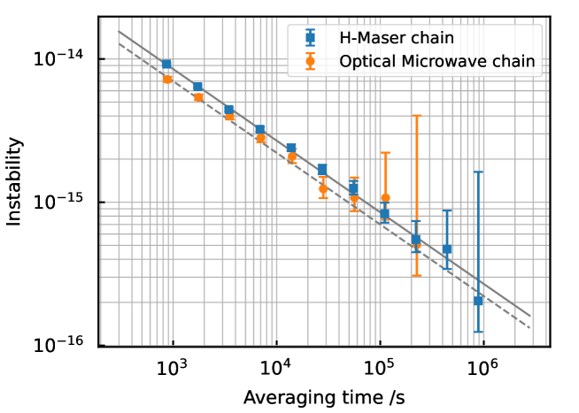
Figure 3: Overlapping Allan deviation of the comparisons over the entire campaign. Orange(blue) dots show data of a measurement carried out using Optical Microwave(H-maser) chain and the dashed(solid) line represents its instability at $$2.1\text{\times}{10}^{-13}$/\sqrt{\tau/$\mathrm{s}$}$ ($$2.7\text{\times}{10}^{-13}$/\sqrt{\tau/$\mathrm{s}$}$).

The instabilities of the comparisons for the entire campaign are shown in Fig. 3 as overlapping Allan deviations. The comparison through the H-maser chain has an instability at $$2.7\text{\times}{10}^{-13}$/\sqrt{\tau/$\mathrm{s}$}$ over the full campaign. The comparison through the Optical Microwave chain has slightly lower instability at $$2.1\text{\times}{10}^{-13}$/\sqrt{\tau/$\mathrm{s}$}$. The improvement is obtained thanks to the lower phase noise of the optically-generated microwave compared to that introduced by the BVA quartz/H-maser system. We have estimated that the contribution of the Dick effect is reduced from $1.6\text{\times}{10}^{-13}\text{\,}$$/\sqrt{\tau/s}$ to a value lower than $3\text{\times}{10}^{-15}\text{\,}$$/\sqrt{\tau/s}$. The best instability observed over a short period of time (less than 1 day) is reduced from $2.1\text{\times}{10}^{-13}\text{\,}$$/\sqrt{\tau/s}$ to $1.3\text{\times}{10}^{-13}\text{\,}$$/\sqrt{\tau/s}$ in high density regime. The residual instability is dominated by the atomic background noise. The average fractional frequency difference between IT-Yb1 and IT-CsF2 is $y(\text{IT-Yb1/IT-CsF2, Optical Microwave chain})=-3.2(3.7)\times 10^{-16}$ as measured with Optical Microwave chain and $y(\text{IT-Yb1/IT-CsF2, H-maser chain})=-3.8(2.9)\times 10^{-16}$ measured with H-maser chain. The statistical uncertainties are respectively $2.8\text{\times}{10}^{-16}$ and $1.6\text{\times}{10}^{-16}$, derived from the instabilities shown in Fig. 3. The weighted average of the two measurements is $y(\text{IT-Yb1/IT-CsF2})=-3.6(2.7)\times 10^{-16}$, that corresponds to an absolute frequency measurement of $f(\text{IT-Yb1})=$518\,295\,836\,590\,863.44(14)\text{\,}\mathrm{H}\mathrm{z}$$.

The measurement is limited by the systematic uncertainty of IT-CsF2, including the density shift calculations, that is $2.3\text{\times}{10}^{-16}$ (Table 2). The uncertainties of IT-Yb1 ($1.9\text{\times}{10}^{-17}$) and the microwave-to-optical conversion at the combs are negligible. With more than one year of data, the statistical uncertainty limited by the fountain instability is reduced below the systematic contribution. In this way, we avoided the need to increase the fountain measurement time by using the H-maser as flywheel [45, 32, 29], and measurements using the H-maser chain and the Optical Microwave chain are handled in the same way.

3.2 Gravitational coupling of fundamental constants

Clock comparisons have been used to constrain the variations of fundamental constants [46, 47]. For example, violations of the Einstein equivalence principle would result in changes in the frequency ratios of atomic clocks. As a possible application, we investigate the coupling of our frequency measurement to the gravitational potential of the sun [2, 48, 49, 50, 45]. We fit the data in Fig. 2a to $y=y_{0}+A\cos\left(2\pi(t-t_{0})/T_{0}\right)$, where $t$ is the date of measurement, $t_{0}$ is the date of the 2022 perihelion, and $T_{0}=$365.26\text{\,}\mathrm{d}$$ is the duration of the anomalistic year. We find $A=-0.0(2.0)\times 10^{-16}$. The amplitude of the annual variation of the gravitational potential is $\Delta\Phi=$1.65\text{\times}{10}^{-10}$c^{2}$, where $c$ is the speed of light. The coupling coefficient of the Yb/Cs ratio to the gravitational potential is then found to be $\beta_{\text{Yb,Cs}}=Ac^{2}/\Delta\Phi=-0.0(1.2)\times 10^{-6}$. This result shows no violation of the Einstein equivalence principle and has a similar uncertainty while being largely independent to the result in Ref. [50]. Following the same approach of Refs. [50, 45] it results in a constrain to the gravitational coupling of the electron-to-proton mass ratio of $k_{\mu}=-0.1(1.2)\times 10^{-6}$. This result can be improved by the continuous long-term operation of frequency standards [47, 2].

4 Conclusions

In this paper, we report the measurement of the clock transition of IT-Yb1 against the primary Cs fountain clock IT-CsF2. The measurement result is $f(\text{IT-Yb1})=$518\,295\,836\,590\,863.44(14)\text{\,}\mathrm{H}\mathrm{z}$$ and the total fractional uncertainty, limited by the systematic uncertainty of IT-CsF2, is $2.7\text{\times}{10}^{-16}$. This is the absolute frequency measurement of Yb against a Cs fountain with the lowest fractional uncertainty. We also show the updated uncertainty budget of IT-Yb1 that has a relative uncertainty of $1.9\text{\times}{10}^{-17}$. In Fig. 4 our measurement reported as a red square is compared to the recommended secondary representations of the second and previous absolute frequency measurements [20, 21, 22, 23, 28, 24, 14, 29, 25, 26, 27, 19, 51], showing a good agreement. Moreover, we note that this measurement supersedes the local frequency measurement we reported in [19], as it extends the analysed data period.

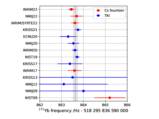
Figure 4: Absolute frequency of Yb performed in several metrological institutes worldwide from 2009 up to now. In red the measurements of Yb against a Cs fountain are shown, while in blue are reported the results of Yb frequency measurements obtained with a link to TAI. The result of the measurement described in this paper is shown as a red square. The grey solid line and shaded area are respectively the recommended secondary representation of the second and its uncertainty, given by CCTF.

These results are a strong demonstration of the improvements achieved in the field of optical clocks and the consequent possibility of introducing a new definition of the second.

References

- [1] Akifumi Takamizawa, Shinya Yanagimachi and Ken Hagimoto “First uncertainty evaluation of the cesium fountain primary frequency standard NMIJ-F2” In Metrologia 59.3 IOP Publishing, 2022, pp. 035004 URL: http://dx.doi.org/10.1088/1681-7575/ac5e7b
- [2] J. Guena et al. “Progress in atomic fountains at LNE-SYRTE” In IEEE Transactions on Ultrasonics, Ferroelectrics, and Frequency Control 59.3, 2012, pp. 391–409 DOI: 10.1109/TUFFC.2012.2208
- [3] Ruoxin Li, Kurt Gibble and Krzysztof Szymaniec “Improved accuracy of the NPL-CsF2 primary frequency standard: evaluation of distributed cavity phase and microwave lensing frequency shifts” In Metrologia 48.5, 2011, pp. 283 DOI: 10.1088/0026-1394/48/5/007
- [4] Scott Beattie et al. “First accuracy evaluation of the NRC-FCs2 primary frequency standard” In Metrologia 57.3 IOP Publishing, 2020, pp. 035010 URL: http://dx.doi.org/10.1088/1681-7575/ab7c54
- [5] S Weyers et al. “Advances in the accuracy, stability, and reliability of the PTB primary fountain clocks” In Metrologia 55.6 IOP Publishing, 2018, pp. 789–805 DOI: 10.1088/1681-7575/aae008
- [6] A Jallageas et al. “First uncertainty evaluation of the FoCS-2 primary frequency standard” In Metrologia 55.3 IOP Publishing, 2018, pp. 366 DOI: 10.1088/1681-7575/aab3fa
- [7] J Guéna et al. “First international comparison of fountain primary frequency standards via a long distance optical fiber link” In Metrologia 54.3 IOP Publishing, 2017, pp. 348–354 DOI: 10.1088/1681-7575/aa65fe
- [8] I.. Blinov et al. “Budget of Uncertainties in the Cesium Frequency Frame of Fountain Type” In Measurement Techniques 60.1, 2017, pp. 30–36 DOI: 10.1007/s11018-017-1145-z
- [9] Fang Fang et al. “NIM5 Cs fountain clock and its evaluation” In Metrologia 52.4 IOP Publishing, 2015, pp. 454–468 DOI: 10.1088/0026-1394/52/4/454
- [10] Filippo Levi et al. “Accuracy evaluation of ITCsF2: a nitrogen cooled caesium fountain” In Metrologia 51.3, 2014, pp. 270 URL: http://stacks.iop.org/0026-1394/51/i=3/a=270
- [11] J Guéna, M Abgrall, A Clairon and S Bize “Contributing to TAI with a secondary representation of the SI second” In Metrologia 51.1, 2014, pp. 108 URL: http://stacks.iop.org/0026-1394/51/i=1/a=108
- [12] Kyle Beloy et al. “Frequency ratio measurements at 18-digit accuracy using an optical clock network” In Nature 591.7851, 2021, pp. 564–569 URL: https://doi.org/10.1038/s41586-021-03253-4
- [13] S.. Brewer et al. “ Quantum-Logic Clock with a Systematic Uncertainty below ” In Physical Review Letters 123 American Physical Society, 2019, pp. 033201 DOI: 10.1103/PhysRevLett.123.033201
- [14] W.. McGrew et al. “Atomic clock performance enabling geodesy below the centimetre level” In Nature 564.7734, 2018, pp. 87–90 URL: https://doi.org/10.1038/s41586-018-0738-2
- [15] Ichiro Ushijima et al. “Cryogenic optical lattice clocks” In Nature Photonics 9.3 Nature Publishing Group, 2015, pp. 185–189 URL: http://dx.doi.org/10.1038/nphoton.2015.5
- [16] Patrick Gill “Is the time right for a redefinition of the second by optical atomic clocks?” In Journal of Physics: Conference Series 723.1, 2016, pp. 012053 URL: http://stacks.iop.org/1742-6596/723/i=1/a=012053
- [17] Jérôme Lodewyck “On a definition of the SI second with a set of optical clock transitions” In Metrologia 56.5 IOP Publishing, 2019, pp. 055009 DOI: 10.1088/1681-7575/ab3a82
- [18] Fritz Riehle, Patrick Gill, Felicitas Arias and Lennart Robertsson “The CIPM list of recommended frequency standard values: guidelines and procedures” In Metrologia 55.2, 2018, pp. 188–200 URL: http://stacks.iop.org/0026-1394/55/i=2/a=188
- [19] C. Clivati et al. “Coherent Optical-Fiber Link Across Italy and France” In Phys. Rev. Applied 18.5 American Physical Society, 2022, pp. 054009 URL: https://link.aps.org/doi/10.1103/PhysRevApplied.18.054009
- [20] N.. Lemke et al. “Spin- Optical Lattice Clock” In Physical Review Letters 103.6 American Physical Society, 2009, pp. 063001 DOI: 10.1103/PhysRevLett.103.063001
- [21] Takuya Kohno et al. “One-Dimensional Optical Lattice Clock with a Fermionic 171Yb Isotope” In Applied Physics Express 2.7 The Japan Society of Applied Physics, 2009, pp. 072501 DOI: 10.1143/APEX.2.072501
- [22] Masami Yasuda et al. “Improved Absolute Frequency Measurement of the 171Yb Optical Lattice Clock towards a Candidate for the Redefinition of the Second” In Applied Physics Express 5.10 The Japan Society of Applied Physics, 2012, pp. 102401 DOI: 10.1143/APEX.5.102401
- [23] Chang Yong Park et al. “Absolute frequency measurement of 1S0()-3P0() transition of 171Yb atoms in a one-dimensional optical lattice at KRISS” In Metrologia 50.2, 2013, pp. 119 URL: http://stacks.iop.org/0026-1394/50/i=2/a=119
- [24] Huidong Kim et al. “Improved absolute frequency measurement of the 171 Yb optical lattice clock at KRISS relative to the SI second” In Japanese Journal of Applied Physics 56.5, 2017, pp. 050302 URL: http://stacks.iop.org/1347-4065/56/i=5/a=050302
- [25] Takumi Kobayashi et al. “Demonstration of the nearly continuous operation of an 171Yb optical lattice clock for half a year” In Metrologia 57.6 IOP Publishing, 2020, pp. 065021 DOI: 10.1088/1681-7575/ab9f1f
- [26] Limeng Luo et al. “Absolute frequency measurement of an Yb optical clock at the 10-16 level using international atomic time” In Metrologia, 2020 URL: http://iopscience.iop.org/10.1088/1681-7575/abb879
- [27] Huidong Kim et al. “Absolute frequency measurement of the 171Yb optical lattice clock at KRISS using TAI for over a year” In Metrologia 58.5 IOP Publishing, 2021, pp. 055007 URL: http://dx.doi.org/10.1088/1681-7575/ac1950
- [28] Marco Pizzocaro et al. “Absolute frequency measurement of the 1S0 3P0 transition of 171Yb” In Metrologia 54.1 IOP Publishing, 2017, pp. 102 DOI: 10.1088/1681-7575/aa4e62
- [29] Marco Pizzocaro et al. “Absolute frequency measurement of the 1S0 3P0 transition of 171Yb with a link to international atomic time” In Metrologia 57.3 IOP Publishing, 2020, pp. 035007 DOI: 10.1088/1681-7575/ab50e8
- [30] Jacopo Grotti et al. “Geodesy and metrology with a transportable optical clock” In Nature Physics 14.5, 2018, pp. 437–441 URL: https://doi.org/10.1038/s41567-017-0042-3
- [31] Marco Pizzocaro et al. “Intercontinental comparison of optical atomic clocks through very long baseline interferometry” In Nature Physics 17.2, 2021, pp. 223–227 URL: https://doi.org/10.1038/s41567-020-01038-6
- [32] Nils Nemitz et al. “Absolute frequency of 87Sr at uncertainty by reference to remote primary frequency standards” In Metrologia 58.2 IOP Publishing, 2021, pp. 025006 URL: http://dx.doi.org/10.1088/1681-7575/abc232
- [33] Gregoire Vallet, Slawomir Bilicki, Rodolphe Le Targat and Jerome Lodewyck “Study of Accuracy and Stability of Sr Lattice Clocks at LNE-SYRTE” In 2018 Conference on Precision Electromagnetic Measurements (CPEM 2018) IEEE, 2018 DOI: 10.1109/cpem.2018.8500833
- [34] R.. Brown et al. “Hyperpolarizability and Operational Magic Wavelength in an Optical Lattice Clock” In Physical Review Letters 119 American Physical Society, 2017, pp. 253001 DOI: 10.1103/PhysRevLett.119.253001
- [35] K. Beloy et al. “Modeling motional energy spectra and lattice light shifts in optical lattice clocks” In Phys. Rev. A 101 American Physical Society, 2020, pp. 053416 DOI: 10.1103/PhysRevA.101.053416
- [36] Nils Nemitz et al. “Modeling light shifts in optical lattice clocks” In Phys. Rev. A 99 American Physical Society, 2019, pp. 033424 DOI: 10.1103/PhysRevA.99.033424
- [37] Pierre Lemonde and Peter Wolf “Optical lattice clock with atoms confined in a shallow trap” In Phys. Rev. A 72 American Physical Society, 2005, pp. 033409 DOI: 10.1103/PhysRevA.72.033409
- [38] J.. Sherman et al. “High-Accuracy Measurement of Atomic Polarizability in an Optical Lattice Clock” In Physical Review Letters 108 American Physical Society, 2012, pp. 153002 DOI: 10.1103/PhysRevLett.108.153002
- [39] J. Lodewyck et al. “Observation and cancellation of a perturbing dc stark shift in strontium optical lattice clocks” In IEEE Trans. Ultrason., Ferroelect., Freq. Cont. 59.3, 2012, pp. 411–415 DOI: 10.1109/tuffc.2012.2209
- [40] Jacques Millo et al. “Ultralow noise microwave generation with fiber-based optical frequency comb and application to atomic fountain clock” In Appl. Phys. Lett. 94, 2009, pp. 141105 DOI: 10.1063/1.3112574
- [41] Burghard Lipphardt, Vladislav Gerginov and Stefan Weyers “Optical Stabilization of a Microwave Oscillator for Fountain Clock Interrogation” In IEEE Transactions on Ultrasonics, Ferroelectrics, and Frequency Control 64.4, 2017, pp. 761–766 DOI: 10.1109/TUFFC.2017.2649044
- [42] Consultative Committee for Time and Frequency (CCTF) “Recommendation CCTF PSFS 2: Updates to the CIPM list of standard frequencies”, 2021 URL: https://www.bipm.org/en/committees/cc/cctf/22-_2-2021
- [43] Jérôme Lodewyck et al. “Universal formalism for data sharing and processing in clock comparison networks” In Phys. Rev. Research 2.4 American Physical Society, 2020, pp. 043269 URL: https://link.aps.org/doi/10.1103/PhysRevResearch.2.043269
- [44] H S Margolis and P Gill “Least-squares analysis of clock frequency comparison data to deduce optimized frequency and frequency ratio values” In Metrologia 52.5, 2015, pp. 628–634 URL: http://stacks.iop.org/0026-1394/52/i=5/a=628
- [45] R. Schwarz et al. “Long term measurement of the clock frequency at the limit of primary Cs clocks” In Phys. Rev. Research 2 American Physical Society, 2020, pp. 033242 DOI: 10.1103/PhysRevResearch.2.033242
- [46] Christian Sanner et al. “Optical clock comparison for Lorentz symmetry testing” In Nature 567.7747, 2019, pp. 204–208 URL: https://doi.org/10.1038/s41586-019-0972-2
- [47] R. Lange et al. “Improved Limits for Violations of Local Position Invariance from Atomic Clock Comparisons” In Phys. Rev. Lett. 126.1 American Physical Society, 2021, pp. 011102 URL: https://link.aps.org/doi/10.1103/PhysRevLett.126.011102
- [48] V.. Dzuba and V.. Flambaum “Limits on gravitational Einstein equivalence principle violation from monitoring atomic clock frequencies during a year” In Phys. Rev. D 95.1 American Physical Society, 2017, pp. 015019 URL: https://link.aps.org/doi/10.1103/PhysRevD.95.015019
- [49] Neil Ashby, Thomas E. Parker and Bijunath R. Patla “A null test of general relativity based on a long-term comparison of atomic transition frequencies” In Nature Physics 14.8, 2018, pp. 822–826 URL: https://doi.org/10.1038/s41567-018-0156-2
- [50] W.. McGrew et al. “Towards the optical second: verifying optical clocks at the SI limit” In Optica 6.4 OSA, 2019, pp. 448–454 DOI: 10.1364/OPTICA.6.000448
- [51] Takumi Kobayashi et al. “Search for Ultralight Dark Matter from Long-Term Frequency Comparisons of Optical and Microwave Atomic Clocks” In Phys. Rev. Lett. 129 American Physical Society, 2022, pp. 241301 DOI: 10.1103/PhysRevLett.129.241301