Dissipation-based WENO stabilization of high-order finite element methods for scalar conservation laws

Abstract

We present a new perspective on the use of weighted essentially nonoscillatory (WENO) reconstructions in high-order methods for scalar hyperbolic conservation laws. The main focus of this work is on nonlinear stabilization of continuous Galerkin (CG) approximations. The proposed methodology also provides an interesting alternative to WENO-based limiters for discontinuous Galerkin (DG) methods. Unlike Runge–Kutta DG schemes that overwrite finite element solutions with WENO reconstructions, our approach uses a reconstruction-based smoothness sensor to blend the numerical viscosity operators of high- and low-order stabilization terms. The so-defined WENO approximation introduces low-order nonlinear diffusion in the vicinity of shocks, while preserving the high-order accuracy of a linearly stable baseline discretization in regions where the exact solution is sufficiently smooth. The underlying reconstruction procedure performs Hermite interpolation on stencils consisting of a mesh cell and its neighbors. The amount of numerical dissipation depends on the relative differences between partial derivatives of reconstructed candidate polynomials and those of the underlying finite element approximation. All derivatives are taken into account by the employed smoothness sensor. To assess the accuracy of our CG-WENO scheme, we derive error estimates and perform numerical experiments. In particular, we prove that the consistency error of the nonlinear stabilization is of the order $p+1/2$, where $p$ is the polynomial degree. This estimate is optimal for general meshes. For uniform meshes and smooth exact solutions, the experimentally observed rate of convergence is as high as $p+1$.

1 Introduction

Many reconstruction-based finite volume and discontinuous Galerkin (DG) methods for hyperbolic problems are designed to adaptively select or blend polynomial approximations corresponding to alternative stencils. Classical representatives of such approaches, such as the essentially nonoscillatory (ENO) schemes developed by Harten et al. [19], use the resulting reconstructions to calculate the Riemann data for high-order extensions of Godunov’s method. Typical requirements for the adaptive selection of stencils/weights include crisp resolution of discontinuities, lack of spurious ripples, and uniformly high accuracy for reconstructions of smooth functions. In weighted ENO (WENO) schemes, convex combinations of candidate polynomials are constructed using normalized smoothness indicators as nonlinear weights [44, 45]. The WENO methodology was introduced by Liu et al. [33] in the context of one-dimensional finite volume approximations. The highly cited paper by Jiang and Shu [23] addressed the aspects of efficient implementation on structured grids in 1D and 2D. The fifth-order WENO scheme proposed in [23] and the underlying smoothness indicator have greatly influenced further research efforts in the field. In contrast to ENO algorithms that use binary weights (0 or 1), the WENO approach produces numerical fluxes that depend continuously on the data.

The development of modern ENO/WENO reconstruction tools for unstructured grids was initiated by Abgrall [1] and Friedrich [15]. Qiu and Shu [41] found that local postprocessing based on WENO reconstructions is an excellent alternative to traditional slope limiting in Runge–Kutta discontinuous Galerkin (DG) methods. Tailor-made algorithms for Hermite WENO (HWENO) limiting in the DG setting were proposed in [36, 38, 52, 53, 54]. Zhang and Shu [47, 48, 49, 50] constrained their WENO reconstructions using a simple scaling limiter that enforces appropriate maximum principles at Legendre Gauss–Lobatto quadrature points and ensures positivity preservation for the evolved cell averages. Detailed reviews of the literature on WENO-DG schemes can be found in [49, 46].

Finite element methods based on high-order continuous Galerkin (CG) approximations do not support the possibility of directly adjusting the gradients of the approximate solution in troubled cells. However, spurious oscillations and violations of discrete maximum principles (DMPs) can be avoided by adding stabilization terms to the baseline discretization. The framework of algebraic flux correction (AFC) makes it possible to guarantee preservation of global and/or local bounds for scalar quantities of interest. The AFC schemes reviewed in [27, 28] use artificial diffusion operators and flux limiting techniques for this purpose. A potential disadvantage compared to WENO-DG approaches lies in the fact that local DMPs impose a second-order accuracy barrier [49], while limiters based on global DMP constraints may fail to prevent nonphysical solution behavior. A possible remedy is the use of smoothness indicators to blend local and global bounds (as proposed, e.g., in [18]).

In this paper, we use HWENO reconstructions to design smoothness sensors for algebraic stabilization of high-order CG schemes. The proposed method introduces high-order dissipation in smooth regions and low-order dissipation in the neighborhood of discontinuities. This design philosophy traces its origins to the classical Jameson–Schmidt–Turkel (JST) scheme [21, 22]. The JST smoothness indicator for 1D schemes is defined using finite difference approximations to the second and first derivatives. Extensions to CG-$\mathbb{P}_{1}$ approximations on unstructured meshes can be found, e.g., in [4, 6, 43]. Barrenechea et al. [5] perform in-depth theoretical investigations of a first-order artificial diffusion method combined with a second-order local projection stabilization (LPS) scheme.

The construction of JST-type stabilization terms for CG and DG methods using polynomials of degree $p>1$ is a more delicate issue. In general, it is essential to ensure that

• high-order (HO) stabilization does not degrade the rates of convergence to smooth solutions and vanishes in the neighborhood of discontinuities;

• low-order (LO) dissipation is strong enough to suppress spurious oscillations but vanishes if the exact solution is a polynomial of degree $p$.

Upper bounds for the viscosity parameters of HO and LO stabilization operators can be obtained by estimating the maximum wave speed as in [2, 31, 35]. Multiplication of the two components by nonnegative weights that add up to one makes it possible to select any convex combination of HO and LO terms. In our method, the HO weight $\gamma_{e}\in[0,1]$ of cell $e$ depends on the difference between (the derivatives of) the evolved finite element solution and a WENO reconstruction. The LO weight is given by $1-\gamma_{e}$. The requirements (i) and (ii) imply that we should use $\gamma_{e}=0$ around shocks and $\gamma_{e}=1$ in cells belonging to smooth regions. Adopting these general design principles, we construct and analyze a nonlinear blend of HO and LO stabilization terms. The results of numerical experiments for standard 1D and 2D test problems illustrate the excellent shock-capturing capabilities of our dissipation-based CG-WENO scheme. Optimal convergence rates are attained for smooth data.

In the next section, we present the generic form of a stabilized CG method for a scalar conservation law. Section 3 introduces a nonlinear blend of HO and LO stabilization terms. In Section 4, we define a WENO-based smoothness indicator. Some details of the employed reconstruction procedures are given in Section 5. The analysis presented in Section 6 yields an optimal $\mathcal{O}(h^{p+1/2})$ estimate of the consistency error. In the last two sections, we show numerical examples and draw conclusions.

2 Stabilized Galerkin discretizations

Let $u(\mathbf{x},t)$ be a scalar conserved quantity depending on the space location $\mathbf{x}\in\bar{\Omega}$ and time instant $t\geq 0$. The Lipschitz boundary of the spatial domain $\Omega\subset\mathbb{R}^{d},\ d\in\{1,2,3\}$ is denoted by $\Gamma=\partial\Omega$. Imposing periodic boundary conditions on $\Gamma$, we consider the initial value problem

$$\frac{\partial u}{\partial t}+\nabla\cdot\mathbf{f}(\mathbf{x},u) =0 \quad\mbox{in}\ \Omega\times(0,T),$$ (1a)

$$u(\cdot,0) =u_{0} \quad\mbox{in}\ \Omega,$$ (1b)

where $u_{0}$ is the initial data and $\mathbf{f}(\mathbf{x},u)$ is the flux function of the conservation law. For example, if $u$ is advected by a given velocity field $\mathbf{v}=\mathbf{v}(\mathbf{x})$, then $\mathbf{f}(\mathbf{x},u)=\mathbf{v}(\mathbf{x})u$. In other hyperbolic problems of the form (1), the flux vector $\mathbf{f}$ may be independent of $\mathbf{x}$ but depend nonlinearly on $u$.

We discretize (1) in space using the continuous Galerkin method on a conforming affine mesh $\mathcal{T}_{h}=\{K_{1},\ldots,K_{E_{h}}\}$. For simplicity, we assume that $\bigcup_{K\in\mathcal{T}_{h}}=\bar{\Omega}$. The mesh size corresponding to $\mathcal{T}_{h}$ is defined by $h=\max_{K\in\mathcal{T}_{h}}h_{K}$, where $h_{K}=\mathrm{diam}(K)$. We seek an approximate solution

$$u_{h}=\sum_{j=1}^{N_{h}}u_{j}\varphi_{j}$$

in a finite element space $V_{h}$ spanned by Lagrange, Bernstein, or Legendre Gauss-Lobatto (LGL) basis functions $\varphi_{1},\ldots,\varphi_{N_{h}}$. The methodology to be presented below is independent of the basis. The polynomial degree of the local finite element approximation $u_{h}^{e}=u_{h}|_{K_{e}}$ is denoted by $p$.

The standard Galerkin discretization of (1) leads to the semi-discrete problem

$$\sum_{e=1}^{E_{h}}\int_{K_{e}}w_{h}\left(\frac{\partial u_{h}}{\partial t}+\nabla\cdot\mathbf{f}(\mathbf{x},u_{h})\right)\mathrm{d}\mathbf{x}=0\qquad\forall w_{h}\in V_{h}.$$ (2)

It is well known that this spatial semi-discretization may not exhibit optimal convergence behavior even if the exact solution $u$ is smooth. Quarteroni and Valli [42, 14.3.1] prove that $\|u-u_{h}\|_{L^{2}(\Omega)}=\mathcal{O}(h^{p})$ for linear advection problems and general meshes. For a properly stabilized CG method, the $L^{2}$ error is $\mathcal{O}(h^{p+1/2})$; see, e.g., [11, 20]. All schemes that we consider below can be written as

$$\sum_{e=1}^{E_{h}}\int_{K_{e}}w_{h}\left(\frac{\partial u_{h}}{\partial t}+\nabla\cdot\mathbf{f}(\mathbf{x},u_{h})\right)\mathrm{d}\mathbf{x}+\sum_{e=1}^{E_{h}}s_{h}^{e}(u_{h},w_{h})=0\qquad\forall w_{h}\in V_{h}.$$ (3)

We discuss some old and new definitions of the local stabilization operator $s_{h}^{e}(\cdot,\cdot)$ in the next section.

Discretization in time can be performed, e.g., using a strong stability preserving (SSP) Runge–Kutta method [16]. The $L^{2}$ error analysis for fully discrete problems confirms the need for adding stabilization terms or using dissipative time stepping (as in Taylor–Galerkin methods [14]).

3 Dissipation-based stabilization

The simplest way to stabilize a scheme that produces spurious oscillations is to add large amounts of isotropic artificial diffusion. We define the corresponding low-order stabilization operator

$$s_{h}^{e,L}(u_{h},w_{h})=\nu_{e}\int_{K_{e}}\nabla w_{h}\cdot\nabla u_{h}\mathrm{d}\mathbf{x}$$ (4)

using the viscosity parameter

$$\nu_{e}=\frac{\lambda_{e}h_{e}}{2p},$$

where $h_{e}$ is the local mesh size and $\lambda_{e}=\|\mathbf{f}^{\prime}(u_{h})\|_{L^{\infty}(K_{e})}$ is an upper bound for the local wave speed.

The use of (4) may be appropriate for cells located in steep front regions. However, stabilization of this kind introduces an $\mathcal{O}(h^{1/2})$ consistency error (see Section 6). A modified version [31, 35] of the two-level variational multiscale (VMS) method proposed by John et al. [24] replaces (4) with

$$s_{h}^{e,H}(u_{h},w_{h})=\nu_{e}\int_{K_{e}}\nabla w_{h}\cdot(\nabla u_{h}-\mathbf{g}_{h})\mathrm{d}\mathbf{x},$$ (5)

where $\mathbf{g}_{h}$ is a continuous approximation to $\nabla u_{h}$. In essence, this stabilization technique adds a linear antidiffusive correction to (4). If $\|\mathbf{g}_{h}-\nabla u_{h}\|_{L^{2}(\Omega)}=\mathcal{O}(h^{p})$, then the consistency error is $\mathcal{O}(h^{p+1/2})$, as we show in Section 6 for a symmetric counterpart of this stabilization operator.

Lohmann et al. [35] discovered an interesting relationship of (5) to a consistent streamline upwind Petrov–Galerkin (SUPG) method [10, 11]. It turned out that the two approaches are equivalent in 1D if $\mathbf{g}_{h}\in(V_{h})^{d}$ is defined as the consistent-mass $L^{2}$ projection of $\nabla u_{h}$, i.e., if

$$\sum_{e=1}^{E_{h}}\int_{K_{e}}w_{h}(\mathbf{g}_{h}-\nabla u_{h})\mathrm{d}\mathbf{x}=0\qquad\forall w_{h}\in V_{h}.$$ (6)

Substituting $w_{h}\in\{\varphi_{1},\ldots,\varphi_{N_{h}}\}$, we find that the nodal values of $\mathbf{g}_{h}=\sum_{j=1}^{N_{h}}\mathbf{g}_{j}\varphi_{j}$ satisfy

$$\sum_{j=1}^{N_{h}}m_{ij}\mathbf{g}_{j}=\sum_{j=1}^{N_{h}}\mathbf{c}_{ij}u_{j},\qquad i=1,\ldots,N_{h},$$

where

$$m_{ij}=\sum_{e=1}^{E_{h}}\int_{K_{e}}\varphi_{i}\varphi_{j}\mathrm{d}\mathbf{x},\qquad\mathbf{c}_{ij}=\sum_{e=1}^{E_{h}}\int_{K_{e}}\varphi_{i}\nabla\varphi_{j}\mathrm{d}\mathbf{x}.$$

To avoid solving linear systems, the coefficients $\mathbf{g}_{i}$ can be redefined as convex combinations

$$\mathbf{g}_{i}=\frac{1}{m_{i}}\sum_{e\in\mathcal{E}_{i}}m_{i}^{e}\nabla u_{h}|_{K_{e}}(\mathbf{x}_{i})$$

of the one-sided limits $\nabla u_{h}|_{K_{e}}(\mathbf{x}_{i})$ in mesh cells $K_{e}$ containing the point $\mathbf{x}_{i}$. The indices of these cells are stored in the set $\mathcal{E}_{i}$. The weights $m_{i}^{e}\geq 0$ must add up to $m_{i}>0$. For example, the positive diagonal entries $m_{i}^{e}=\int_{K_{e}}\varphi_{i}\mathrm{d}\mathbf{x}$ of the lumped element mass matrix can be used in the context of Bernstein finite element approximations. This definition was adopted in [31], and the corresponding operator $s_{h}^{e,H}(\cdot,\cdot)$ was found to be well suited for linear stabilization purposes.

The bilinear form of the VMS stabilization term (5) is nonsymmetric. As a consequence, its contribution to (3) may produce entropy [31]. The symmetric version

$$s_{h}^{e,H}(u_{h},w_{h})=\nu_{e}\int_{K_{e}}(\nabla w_{h}-\mathbf{g}_{h}(w_{h}))\cdot(\nabla u_{h}-\mathbf{g}_{h}(u_{h}))\mathrm{d}\mathbf{x}$$ (7)

is truly dissipative because it is coercive in the sense that $s_{h}^{e,H}(v_{h},v_{h})\geq 0\ \forall v_{h}\in V_{h}$. Projection-based stabilization operators of this type were proposed, for instance, in [9, 12]. In the numerical experiments of Section 7, we use formula (7) with $\mathbf{g}_{h}$ defined by (6).

As announced in the introduction, our objective is to combine a low-order stabilization operator and a high-order one in order to construct a multidimensional high-order CG-WENO version of the JST scheme [22]. Introducing a blending factor $\gamma_{e}\in[0,1]$, we define (cf. [5])

$$s_{h}^{e}(u_{h},w_{h}) =\omega\gamma_{e}\nu_{e}\int_{K_{e}}(\nabla w_{h}-\pi_{h}\nabla w_{h})\cdot(\nabla u_{h}-\pi_{h}\nabla u_{h})\mathrm{d}\mathbf{x},$$

$$+(1-\gamma_{e})\nu_{e}\int_{K_{e}}\nabla w_{h}\cdot\nabla u_{h}\mathrm{d}\mathbf{x}.$$ (8)

The additional parameter $\omega\in[0,1]$ can be used to adjust the levels of high-order dissipation as in [31, 35]. Note that $s_{h}^{e}(u_{h},w_{h})$ defined by (8) reduces to (4) for $\gamma_{e}=0$ and to (7) for $\gamma_{e}=1=\omega$.

According to the JST design philosophy, $\gamma_{e}$ should approach 0 in troubled cells and 1 in smooth ones. The same blending strategy can be applied to other pairs of stabilization operators $s_{h}^{e,L}$ and $s_{h}^{e,H}$ as long as the latter is accuracy preserving and the former is sufficiently dissipative. In the case $p=1$, the theoretical framework developed by Barrenechea et al. [5, 6, 8] can be used to prove the validity of a discrete maximum principle for specific choices of $\gamma_{e}$ and $s_{h}^{e,L}$. Numerical schemes of order $q>2$ cannot be locally bound preserving in general [49]. However, preservation of global bounds does not impose an order barrier. Zhang and Shu [47, 48, 49, 50] introduced a simple scaling limiter that makes a high-order DG-WENO scheme positivity preserving. In the CG setting, the element-based limiters developed in [13, 30, 28, 35] can be used to enforce positivity preservation in a similar way.

4 Smoothness sensor

Many shock-capturing methods and selective limiting techniques for finite element schemes are equipped with smoothness indicators for detection of troubled cells (see, e.g., [18, 25, 35, 40]). In principle, any of these shock detectors can be used to define $\gamma_{e}$ for (8). However, not all of the resulting hybrid schemes will meet the conflicting demands for high-order accuracy and strong stability. Motivated by the tremendous success of WENO schemes in the context of finite volume and DG methods, we define our dissipation-based stabilization term (8) using the smoothness sensor

$$\gamma_{e}=1-\min\bigg{(}1,\frac{\|u_{h}^{e}-u_{h}^{e,*}\|_{e}}{\|u_{h}^{e}\|_{e}}\bigg{)}^{q},$$ (9)

where $u_{h}^{e}=u_{h}|_{K_{e}}$ and $u_{h}^{e,*}$ is a WENO reconstruction. The choice of $q\geq 1$ determines how sensitive $\gamma_{e}$ is to the relative difference between $u_{h}^{e}$ and $u_{h}^{e,*}$. The norm $\|\cdot\|_{e}$ is defined similarly to smoothness indicators for WENO schemes. In this work, we use the scaled Sobolev semi-norm (cf. [15, 23])

$$\|v\|_{e}=\left(\sum_{1\leq|\mathbf{k}|\leq p}h_{e}^{2|\mathbf{k}|-d}\int_{K_{e}}|D^{\mathbf{k}}v|^{2}\mathrm{d}\mathbf{x}\right)^{1/2}\qquad\forall v\in H^{p}(K_{e}).$$ (10)

In this formula, $\mathbf{k}=(k_{1},\ldots,k_{d})$ is the multiindex of the partial derivative

$$D^{\mathbf{k}}v=\frac{\partial^{|\mathbf{k}|}v}{\partial x_{1}^{k_{1}}\cdots\partial x_{d}^{k_{d}}},\qquad|\mathbf{k}|=k_{1}+\ldots+k_{d}.$$

Remark 1.

Derivative-based metrics of the form $\|\cdot\|_{e}^{q},\ q\in\{1,2\}$ were used to measure the smoothness of candidate polynomials by Jiang and Shu [23] and Friedrich [15]. Our definition of the blending parameter $\gamma_{e}\in[0,1]$ supports the possibility of raising $\|\cdot\|_{e}$ to a user-defined power $q\geq 1$.

Remark 2.

In contrast to WENO-based slope limiting approaches, we do not overwrite $u_{h}^{e}$ by $u_{h}^{e,*}$ in troubled cells. The reconstruction is used only to calculate $\gamma_{e}$ for the dissipative stabilization term (8). The evolution of $u_{h}$ is governed by (3). Thus the semi-discrete problem has the structure of a GG method, while overwriting DG approaches have more in common with finite volume methods.

5 WENO reconstruction

The computation of $u_{h}^{e,*}$ is based on the same methodology as WENO averaging of candidate polynomials in finite volume [15, 23] and Runge–Kutta discontinuous Galerkin [36, 51, 52, 54] methods. The main idea is to blend several approximations using a smoothness sensor to assign larger weights to less oscillatory polynomials. In the finite element context, convex combinations of Lagrange and/or Hermite polynomials corresponding to different stencils can be constructed in this way.

To facilitate the reproducibility of the numerical results to be presented in Section 7, we outline the employed reconstruction procedure without claiming originality or superiority to existing alternatives. The main added value of our work is not the way to calculate the WENO polynomials $u_{h}^{e,*}$ but the manner in which we use them to stabilize the underlying CG scheme (see above).

Let $K_{e}\in\mathcal{T}_{h}$ be a generic mesh cell and $u_{h}$ a finite element approximation from the previous iteration, (pseudo-)time step, or Runge–Kutta stage. To measure the smoothness of $u_{h}^{e}$ on $K_{e}$, we need to construct a polynomial $u_{h}^{e,*}$ that has the same degree $p\geq 1$ and is free of spurious oscillations. We denote by $\mathcal{S}^{e}$ the integer set containing the indices $e^{\prime}$ of all neighbor cells $K_{e^{\prime}}\in\mathcal{T}_{h}$ that provide data for the computation of $u_{h}^{e,*}$. Note that $e\in\mathcal{S}^{e}$ by definition. For $l=1,\ldots,m_{e}$, we define a stencil $\mathcal{S}^{e}_{l}$ as a subset of $\mathcal{S}^{e}$ and reconstruct a candidate polynomial $u_{h,l}^{e}$ from the restriction of $u_{h}$ to the patch $\bar{\Omega}_{l}^{e}=\bigcup_{e^{\prime}\in\mathcal{S}_{l}^{e}}K_{e^{\prime}}$. The identity mapping $u_{h,0}^{e}=u_{h}^{e}$ corresponds to the stencil $\mathcal{S}_{0}^{e}=\{e\}$.

The properties of a reconstructed polynomial $u_{h,l}^{e}$ depend on the choice of the stencil. To achieve high-order accuracy and stability in regions where the solution is sufficiently smooth, stencils that are centered w.r.t. $K_{e}$ should be included. On the other hand, one-sided stencils are needed to avoid strong oscillations around discontinuities. The number of stencils should be as small as possible to minimize the computational cost. However, it must be sufficiently large to ensure the existence of nonoscillatory candidate polynomials. An important advantage of high-order finite element methods (compared to Godunov-type finite volume schemes) is that not only cell averages but also partial derivatives of degree up to $p$ are available. Hence, direct neighbors of $K_{e}$ typically provide enough data.

When it comes to the construction of candidate polynomials $u_{h,l}^{e}$, we have a choice between least-squares fitting and interpolation. The latter approach is more common in the finite element setting. The cell averages / pointwise values of Lagrange interpolation polynomials and (some) partial derivatives of Hermite interpolation polynomials match those of $u_{h}$ in cells belonging to reconstruction stencils. The HWENO limiter developed by Luo et al. [36] for DG-$\mathbb{P}_{1}$ approximations on simplex meshes combines $d+1$ linear Lagrange polynomials and $d+2$ linear Hermite polynomials. The reconstruction procedure is simple and efficient, especially if the Taylor basis [37] is used to represent $u_{h}$. The approach proposed by Zhong and Shu [51] extends the DG polynomials $u_{h}^{e^{\prime}}$ of neighbor cells $e^{\prime}\in\mathcal{S}^{e}_{l}$ into $K_{e}$ and corrects the average. We use this kind of Hermite interpolation and give some details below.

The vertex neighborhood of $K_{e}$ is the set of all cells that have a common vertex with $K_{e}$. In our implementation, we use only cells belonging to the von Neumann neighborhood. That is, an index $e^{\prime}$ belongs to $\mathcal{S}^{e}$ if $K_{e}$ and $K_{e^{\prime}}$ have a common boundary (a point in 1D, an edge in 2D, a face in 3D). Since $e\in\mathcal{S}^{e}$, we can use $\mathcal{S}_{0}^{e}=\{e\}$ and $m_{e}\geq d+1$ reconstruction stencils $S_{l}^{e}=\{e,e^{\prime}\}$, where $e^{\prime}\in\mathcal{S}^{e}\backslash\{e\}$. Using the local basis functions of element $e^{\prime}$ and the corresponding degrees of freedom, we define a polynomial $u_{h}^{e^{\prime}}$, which can be evaluated at $\mathbf{x}\in K_{e}$ to construct (cf. [51])

$$u_{h,l}^{e}(\mathbf{x})=u_{h}^{e^{\prime}}(\mathbf{x})+\pi_{e}(u_{h}^{e}-u_{h}^{e^{\prime}}),\qquad\mathbf{x}\in K_{e},$$ (11)

where $\pi_{e}v=\frac{1}{|K_{e}|}\int_{K_{e}}v\mathrm{d}\mathbf{x}$ denotes the average value of $v\in\{u_{h}^{e},u_{h}^{e^{\prime}}\}$ in $K_{e}$. The so-defined candidate polynomials $u_{h,l}^{e}$ correspond to a Hermite WENO reconstruction such that

$$\pi_{e}u_{h,l}^{e}=\pi_{e}u_{h}^{e},\qquad D^{\mathbf{k}}u_{h,l}^{e}=D^{\mathbf{k}}u_{h}^{e^{\prime}},\qquad 1\leq|\mathbf{k}|\leq p.$$

If the approximation $u_{h}$ varies smoothly on all cells with indices in $\mathcal{S}^{e}$, then a convex combination

$$\tilde{u}_{h}^{e}=\sum_{l=0}^{m_{e}}\tilde{\omega}_{l}^{e}u_{h,l}^{e}\in\mathbb{P}_{p}(K_{e})$$

of candidate polynomials can be defined using linear weights $\tilde{\omega}_{l}^{e}\in[0,1]$. In finite volume methods, the choice of $\tilde{\omega}_{l}^{e}$ is optimal if it maximizes the accuracy of reconstructed interface values at flux evaluation points. For example, the linear component of the WENO scheme proposed by Jiang and Shu [23] yields a fifth-order approximation that represents a convex average of three third-order approximations. In the finite element context, small positive weights $\tilde{\omega}_{l}^{e}$ may be assigned to $u_{h,l}^{e},\ l=1,\ldots,m_{e}$ and a large weight $\tilde{\omega}_{0}^{e}=1-\sum_{l=1}^{m_{e}}\tilde{\omega}_{l}^{e}$ to $u_{h,0}^{e}=u_{h}^{e}$. Such definitions can be found, e.g., in [51, 54]. Since our smoothness indicator measures deviations from the WENO reconstruction, assigning a smaller linear weight to $u_{h,0}^{e}$ results in more reliable shock detection and stronger nonlinear stabilization.

Since $\tilde{u}_{h}^{e}$ may be oscillatory, the nonlinear weights ${\omega}_{l}^{e}\in[0,1]$ of an adaptive WENO reconstruction

$$\tilde{u}_{h}^{e,*}=\sum_{l=0}^{m_{e}}{\omega}_{l}^{e}u_{h,l}^{e}\in\mathbb{P}_{p}(K_{e})$$

are commonly defined using linear weights $\tilde{\omega}_{l}^{e}$ and smoothness sensors $\beta_{l}^{e}$ such as

$$\beta_{l}^{e}=\|u_{h,l}^{e}\|_{e}^{q},\qquad q\geq 1,$$

where $\|\cdot\|_{e}$ is the semi-norm defined by (10). The classical smoothness indicators proposed by Jiang and Shu [23] and Friedrich [15] use $q=2$ in 1D and $q=1$ in 2D, respectively.

A popular definition of the nonlinear weights $\omega_{l}^{e}$ for a WENO scheme is given by [23, 52, 54]

$$\omega_{l}^{e}=\frac{\tilde{w}_{l}^{e}}{\sum_{k=0}^{m_{e}}\tilde{w}_{k}^{e}},\qquad\tilde{w}_{l}^{e}=\frac{\tilde{\omega}_{l}^{e}}{(\epsilon+\beta_{l}^{e})^{r}}.$$

Here $r$ is a positive integer and $\epsilon$ is a small positive real number, which is added to avoid division by zero. In our implementation, we use the parameter settings $r=2$ and $\epsilon=10^{-6}$.

Remark 3.

By definition (10) of the semi-norm $\|\cdot\|_{e}$, our WENO-based smoothness indicator (9) depends only on the derivatives of candidate polynomials. The correction of cell averages by adding $\pi_{e}(u_{h}^{e}-u_{h}^{e^{\prime}})$ to $u_{h}^{e^{\prime}}(\mathbf{x})$ in (11) has no influence on the value of $\gamma_{e}$ and is, therefore, unnecessary in practice (in contrast to DG-WENO schemes that overwrite $u_{h}^{e}$ by $u_{h}^{e,*}$).

Remark 4.

Additional Hermite polynomials can be generated by including further stencils of the form $\{l,m\}$ such that $K_{l}$ and $K_{m}$ share a vertex with $K_{e}$. Moreover, Lagrange interpolation polynomials may be constructed. In the context of HWENO slope limiting for piecewise-linear DG approximations, Luo et al. [36] interpolate the values of $u_{h}$ at the barycenters of $d+1$ cells belonging to the reconstruction stencil $S_{l}^{e}$. In general, each mesh element has $N_{K}$ vertices. Let $S_{l}^{e}$ contain the indices of $N_{K}$ cells that surround a vertex of $K_{e}$. Define $K_{e,l}$ as the convex hull of the barycenters of these cells. Then a candidate polynomial of degree $p\geq 1$ can be constructed by interpolating the values of $u_{h}$ at the nodal points of a $p$th degree Lagrange finite element approximation on $K_{e,l}$. This reconstruction strategy generalizes the methodology proposed in [36] to arbitrary-order finite elements.

In DG schemes equipped with Hermite WENO limiters, troubled cell indicators are commonly employed to minimize the cost incurred by polynomial reconstructions (see, e.g., [51, 53]). Clearly, we also have the option of skipping the calculation of $u_{h}^{e,*}$ and setting $\gamma_{e}\equiv 1$ in cells identified as smooth by an inexpensive (but safe) shock detector. To better understand the behavior of dissipation-based WENO stabilization, we do not attempt to localize it in this way in the present paper.

6 Error estimates

Following the theoretical investigations of algebraic flux correction schemes in [7, 8] and [34, Chap. 4], we perform preliminary error analysis of nonlinear dissipation-based WENO stabilization for the continuous Galerkin discretization of the linear Dirichlet boundary-value problem

$$\mathbf{v}\cdot\nabla u+cu =f \quad\mbox{in}\ \Omega,$$ (12a)

$$u =0 \quad\mbox{on}\ \Gamma_{-},$$ (12b)

where $\Gamma_{-}$ is the inflow boundary of $\Omega\subset\mathbb{R}^{d}$ and $\mathbf{v}\in[\mathrm{Lip}(\Omega)]^{d}$ is a Lipschitz-continuous velocity field. The given functions $c\in L^{\infty}(\Omega)$ and $f\in L^{2}(\Omega)$ determine the intensity of reactive terms. To ensure the well-posedness of continuous and discrete problems, we make the usual assumption that

$$\exists c_{0}>0:\quad c-\frac{1}{2}\nabla\cdot\mathbf{v}\geq c_{0}\qquad\mbox{a.e. in}\ \Omega.$$ (13)

A stabilized Galerkin discretization of (12) is given by

$$a(u_{h},w_{h})+s_{h}(u_{h};u_{h},w_{h})=b(w_{h})\qquad\forall w_{h}\in V_{h},$$ (14)

where [34, Chap. 2]

$$a(u,w):=\int_{\Omega}(w\mathbf{v}\cdot\nabla u+cwu)\mathrm{d}\mathbf{x}-\int_{\Gamma}wu\min(0,\mathbf{v}\cdot\mathbf{n})\mathrm{d}\mathbf{s},$$

$$b(w):=\int_{\Omega}wf\mathrm{d}\mathbf{x}.$$

In the integral over $\Gamma$, we denote by $\mathbf{n}$ the unit outward normal. Using $\eqref{stab:WENO}$ with $\omega=1$, we define

$$s_{h}(u_{h};v_{h},w_{h}) =\sum_{e=1}^{E_{h}}\gamma_{e}(u_{h})\nu_{e}\int_{K_{e}}(\nabla w_{h}-\pi_{h}\nabla w_{h})\cdot(\nabla v_{h}-\pi_{h}\nabla v_{h})\mathrm{d}\mathbf{x}$$

$$+\sum_{e=1}^{E_{h}}(1-\gamma_{e}(u_{h}))\nu_{e}\int_{K_{e}}\nabla w_{h}\cdot\nabla u_{h}\mathrm{d}\mathbf{x}.$$

For any fixed $u_{h}\in V_{h}$, the mapping $s_{h}(u_{h};\cdot,\cdot)$ is a symmetric bilinear form which is positive semi–definite and, therefore, satisfies the Cauchy–Schwarz inequality (cf. [7, eq. (41)])

$$s_{h}(u_{h};v_{h},w_{h})\leq\sqrt{s_{h}(u_{h};v_{h},v_{h})}\sqrt{s_{h}(u_{h};w_{h},w_{h})}\qquad\forall v_{h},w_{h}\in V_{h}.$$ (15)

To measure the difference $e=u-u_{h}$ between a solution $u_{h}\in V_{h}$ of the discrete problem (14) and an exact weak solution $u\in H^{p+1}(\Omega)$ of the continuous problem (12), we will use the norms

$$\|e\|_{a}^{2}=c_{0}\|e\|_{L^{2}(\Omega)}^{2}+\tfrac{1}{2}\int_{\Gamma}e^{2}|\mathbf{v}\cdot\mathbf{n}|\mathrm{d}\mathbf{s},\qquad\|e\|_{h}^{2}=\|e\|_{a}^{2}+s_{h}(u_{h};I_{h}e,I_{h}e),$$

where $I_{h}:C(\bar{\Omega})\to V_{h}$ is the interpolation operator. Since $s_{h}(u_{h};\cdot,\cdot)$ has the same properties as the AFC stabilization operator $d_{h}(u_{h};\cdot,\cdot)$ considered in [7, 8, 34], we have

$$\|u-u_{h}\|_{h}\leq\inf_{v\in V_{h}}\Big{(}\|u-v_{h}\|_{h}+\sup_{w_{h}\in V_{h}}\frac{a(u-v_{h},w_{h})}{\|w_{h}\|_{h}}+\sqrt{s_{h}(u_{h};v_{h},v_{h})}\Big{)}.$$

In essence, this result is an adaptation of Strang’s first lemma to stabilized Galerkin schemes. Choosing $v_{h}=I_{h}u$ and following Lohmann [34, Lemma 4.71], we deduce that

$$\|u-u_{h}\|_{h}\leq\|u-I_{h}u\|_{a}+\sup_{w_{h}\in V_{h}}\frac{a(u-I_{h}u,w_{h})}{\|w_{h}\|_{h}}+\sqrt{s_{h}(u_{h};I_{h}u,I_{h}u)}.$$ (16)

An $\mathcal{O}(h^{p})$ bound for the sum of the first two terms on the right-hand of this inequality can be derived as in [20, 34]. The last term measures the consistency error due to nonlinear stabilization.

Recall that $\nu_{e}=\mathcal{O}(h)$ and $\gamma_{e}\in[0,1]$. If the exact weak solution $u$ is sufficiently smooth, then

$$\sum_{e=1}^{E_{h}}\gamma_{e}(u_{h})\nu_{e}\int_{K_{e}}|\nabla I_{h}u-\pi_{h}\nabla I_{h}u|^{2}\mathrm{d}\mathbf{x}\leq Ch\sum_{e=1}^{E_{h}}\int_{K_{e}}|\nabla I_{h}u|^{2}\mathrm{d}\mathbf{x}=Ch\|\nabla I_{h}u\|_{L^{2}(\Omega)}^{2}.$$

The low-order component is bounded similarly. Hence, $\sqrt{s_{h}(u_{h};I_{h}u,I_{h}u)}=\mathcal{O}(h^{1/2})$ in the worst case.

On the other hand, suppose that the high-order component dominates and the estimate

$$\sum_{e=1}^{E_{h}}(1-\gamma_{e}(u_{h}))\nu_{e}\int_{K_{e}}|\nabla I_{h}u|^{2}\mathrm{d}\mathbf{x} \leq Ch\sum_{e=1}^{E_{h}}\int_{K_{e}}|\nabla I_{h}u-\pi_{h}\nabla I_{h}u|^{2}\mathrm{d}\mathbf{x}$$

$$=Ch\|\nabla I_{h}u-\pi_{h}\nabla I_{h}u\|_{L^{2}(\Omega)}^{2}$$

holds a posteriori for a specific choice of $\gamma_{e}$. Using the triangle inequality, we find that

$$\|\nabla I_{h}u-\pi_{h}\nabla I_{h}u\|_{L^{2}(\Omega)}\leq\|\nabla I_{h}u-\nabla u\|_{L^{2}(\Omega)}+\|\nabla u-\pi_{h}\nabla u\|_{L^{2}(\Omega)}+\|\pi_{h}(\nabla u-I_{h}\nabla u)\|_{L^{2}(\Omega)},\quad$$

where

$$\|\nabla I_{h}u-\nabla u\|_{L^{2}(\Omega)}=|I_{h}u-u|_{H^{1}(\Omega)}\leq Ch^{p}|u|_{H^{p+1}(\Omega)}.$$

If $\pi_{h}$ is the $L^{2}$ projection operator, then its best approximation property implies that

$$\|\pi_{h}\nabla u-\nabla u\|_{L^{2}(\Omega)}\leq\|I_{h}\nabla u-\nabla u\|_{L^{2}(\Omega)}\leq Ch^{p}|\nabla u|_{H^{p}(\Omega)}.$$

Since $\|\pi_{h}v\|_{L^{2}(\Omega)}^{2}=(v,\pi_{h}v)_{L^{2}(\Omega)}$ for $v\in L^{2}(\Omega)$, we can use the Cauchy–Schwarz inequality and Young’s inequality to show that $\|\pi_{h}v\|_{L^{2}(\Omega)}\leq\|v\|_{L^{2}(\Omega)}$ for any $v\in L^{2}(\Omega)$. Combining the above auxiliary results, we conclude that $\sqrt{s_{h}(u_{h};I_{h}u,I_{h}u)}=\mathcal{O}(h^{p+1/2})$ under our assumption that the high-order stabilization is dominant for the particular choice of $\gamma_{e}(u_{h})$.

Remark 5.

An optimal $\mathcal{O}(h^{p+1/2})$ a priori error estimate for the linear high-order scheme can be obtained following the analysis of the SUPG method in [20, 28]. Instead of $\tau h\|\mathbf{v}\cdot\nabla\rho\|_{L^{2}(\Omega)}$, where $\rho=u-I_{h}u$ is the interpolation error and $\tau$ is the SUPG stabilization parameter, the estimate will contain $\sqrt{s_{h}(u_{h};I_{h}u,I_{h}u)}$ with $\gamma_{e}\equiv 1$. This term is $\mathcal{O}(h^{p+1/2})$, as shown above.

Remark 6.

If the restriction of $u_{h}$ to the union of mesh cells with indices in $\mathcal{S}^{e}$ is a polynomial of degree up to $p$, then $\|u_{h}^{e}-u_{h}^{e,*}\|_{e}=0$ and $\gamma_{e}(u_{h})=1$ for any choice of the nonlinear weights. Therefore, polynomial exact solutions can be reproduced exactly by our method.

For a general smooth function $u\in C^{p+1}(\bar{\Omega})$, we claim that the WENO consistency error satisfies

$$\sqrt{s_{h}(I_{h}u;I_{h}u,I_{h}u)}=\mathcal{O}(h^{p+1/2}).$$ (17)

To prove the validity of this claim, we need to estimate $\|v_{h}^{e}-v_{h}^{e,*}\|_{e}$ for $v_{h}=I_{h}u$. The multivariate Taylor expansions of the Hermite candidate polynomials $v^{e}_{h,l}$ are given by

$$v^{e}_{h,l}(\mathbf{x})=v^{e}_{l}+\sum_{1\leq|\mathbf{m}|\leq p}D^{\mathbf{m}}u(\mathbf{x}^{e}_{l})\frac{(\mathbf{x}-\mathbf{x}^{e}_{l})^{\mathbf{m}}}{\mathbf{m}!},$$

where we use the multiindex notation. For $e^{\prime}\in\mathcal{S}_{l}^{e}$, we denote by $\mathbf{x}^{e}_{l}$ the centroid $\pi_{e^{\prime}}\mathbf{x}$ of $K_{e^{\prime}}$. The value of the constant $v^{e}_{l}=v^{e}_{h,l}(\mathbf{x}^{e}_{l})$ is uniquely determined by the requirement that $v^{e}_{h,l}$ have the cell average $\pi_{e}v^{e}_{h,l}=\pi_{e}v^{e}_{h}=\pi_{e}I_{h}u$. By definition of $\|\cdot\|_{e}$ and $v_{h}^{e,*}$, we have

$$\|v_{h}^{e}-v_{h}^{e,*}\|_{e}^{2}=\sum_{1\leq|\mathbf{k}|\leq p}h_{e}^{2|\mathbf{k}|-d}\int_{K_{e}}\left|\sum_{l=1}^{m_{e}}\omega_{l}^{e}D^{\mathbf{k}}(v^{e}_{h,l}-v^{e}_{h,0})\right|^{2}\mathrm{d}\mathbf{x}.$$ (18)

Introducing the Taylor basis functions [37]

$$\psi^{e}_{\mathbf{m}}(\mathbf{x})=\frac{1}{\mathbf{m}!}\left[(\mathbf{x}-\mathbf{x}^{e}_{0})^{\mathbf{m}}-\frac{1}{|K_{e}|}\int_{K_{e}}(\mathbf{x}-\mathbf{x}^{e}_{0})^{\mathbf{m}}\mathrm{d}\mathbf{x}\right]$$

such that

$$v^{e}_{h,l}(\mathbf{x})=\pi_{e}v^{e}_{h,l}+\sum_{1\leq|\mathbf{m}|\leq p}D^{\mathbf{m}}v^{e}_{h,l}(\mathbf{x}^{e}_{0})\psi^{e}_{\mathbf{m}}(\mathbf{x}),$$

we proceed to estimate

$$D^{\mathbf{k}}v^{e}_{h,l}(\mathbf{x})-D^{\mathbf{k}}v^{e}_{h,0}(\mathbf{x})=\left(\sum_{l=1}^{m_{e}}\omega_{l}^{e}\sum_{1\leq|\mathbf{m}|\leq p}[D^{\mathbf{m}}v^{e}_{h,l}(\mathbf{x}^{e}_{0})-D^{\mathbf{m}}u(\mathbf{x}^{e}_{0})]\right)D^{\mathbf{k}}\psi^{e}_{\mathbf{m}}(\mathbf{x}).$$

By definition of the candidate polynomials $v^{e}_{h,l},\ l\in\{1,\ldots,m_{e}\}$, the difference

$$R^{e}_{\mathbf{m},l}(\mathbf{x})=D^{\mathbf{m}}v^{e}_{h,l}(\mathbf{x})-D^{\mathbf{m}}u(\mathbf{x})$$

is the remainder of a truncated Taylor expansion of $D^{\mathbf{m}}u(\mathbf{x})$ about the centroid $\mathbf{x}^{e}_{l}$. The degree of the Taylor polynomial $D^{\mathbf{m}}v^{e}_{h,l}(\mathbf{x}^{e}_{0})$ is $p-|\mathbf{m}|\geq 0$. It follows that

$$|R^{e}_{\mathbf{m},l}(\mathbf{x}^{e}_{0})|=\mathcal{O}(h^{p-|\mathbf{m}|+1}).$$

Invoking the definition of $\psi^{e}_{\mathbf{m}}$, we deduce that $|D^{\mathbf{k}}\psi^{e}_{\mathbf{m}}(\mathbf{x})|=\mathcal{O}(h^{|\mathbf{m}|-|\mathbf{k}|})$ for $|\mathbf{x}-\mathbf{x}^{e}_{0}|\leq Ch$. Thus

$$|D^{\mathbf{k}}v^{e}_{h,l}(\mathbf{x})-D^{\mathbf{k}}v^{e}_{h,0}(\mathbf{x})|=\mathcal{O}(h^{p-|\mathbf{k}|+1}).$$

Using this result and the fact that $|K_{e}|=\mathcal{O}(h^{d})$ to estimate the right-hand side of (18), we arrive at

$$\|v_{h}^{e}-v_{h}^{e,*}\|_{e}^{2}=\mathcal{O}(h^{2p+2}).$$

Let the smoothness indicator $\gamma_{e}(v_{h})$ be defined by formula (9) with $q=2$. Then

$$(1-\gamma_{e}(v_{h}))\nu_{e}\int_{K_{e}}|v_{h}|^{2}\mathrm{d}\mathbf{x} =\nu_{e}\min\left(1,\frac{\|v_{h}^{e}-v_{h}^{e,*}\|_{e}^{2}}{\|v_{h}^{e}\|_{e}^{2}}\right)\|v_{h}^{e}\|_{L^{2}(\Omega)}^{2}$$

$$\leq C\nu_{e}h^{d-2}\min\left(\|v_{h}^{e}-v_{h}^{e,*}\|_{e}^{2},\|v_{h}^{e}\|_{e}^{2}\right),$$

where $\nu_{e}=\mathcal{O}(h)$ and $\|v_{h}^{e}\|_{e}=\mathcal{O}(1)$. Hence, the low-order component of $s_{h}(I_{h}u;I_{h}u,I_{h}u)$ is $\mathcal{O}(h^{2p+1})$. The corresponding estimate for the high-order component was obtained above. This proves the validity of our claim that the consistency error of the WENO stabilization satisfies (17).

The nonlinear term that appears in (16) is not $s_{h}(I_{h}u;I_{h}u,I_{h}u)$ but $s_{h}(u_{h};I_{h}u,I_{h}u)$. To obtain a final a priori error estimate, let us assume that the Lipschitz continuity condition

$$|s_{h}(u_{h};v_{h},v_{h})-s_{h}(v_{h};v_{h},v_{h})|\leq s_{h}(u_{h};v_{h}-u_{h},v_{h}-u_{h})\qquad\forall u_{h}\in V_{h}$$

holds for the interpolant $v_{h}=I_{h}u$ of $u\in C^{p+1}(\bar{\Omega})$. Then (16) implies

$$\|u-u_{h}\|_{a} =\|u-u_{h}\|_{h}-\sqrt{s_{h}(u_{h};I_{h}u-u_{h},I_{h}u-u_{h})}$$

$$\leq\|u-I_{h}u\|_{a}+\sup_{w_{h}\in V_{h}}\frac{a(u-I_{h}u,w_{h})}{\|w_{h}\|_{h}}-\sqrt{s_{h}(u_{h};I_{h}u-u_{h},I_{h}u-u_{h})}$$

$$+\sqrt{s_{h}(u_{h};I_{h}u-u_{h},I_{h}u-u_{h})+s_{h}(I_{h}u;I_{h}u,I_{h}u)}$$

$$\leq\|u-I_{h}u\|_{a}+\sup_{w_{h}\in V_{h}}\frac{a(u-I_{h}u,w_{h})}{\|w_{h}\|_{h}}+\sqrt{s_{h}(I_{h}u;I_{h}u,I_{h}u)}.$$

The last term on the right-hand side of this inequality can be now be estimated using (17). As already mentioned, an $\mathcal{O}(h^{p})$ estimate is available for the sum of the first two terms.

Remark 7.

Barrenechea et al. [8] use similar arguments to derive an improved a priori error estimate for algebraic flux correction schemes equipped with linearity-preserving limiters.

7 Numerical examples

In this section, we present the results of some numerical experiments for linear and nonlinear scalar problems. The objective of our study is to show that the CG-WENO scheme

• exhibits optimal convergence behavior for problems with smooth solutions;

• introduces sufficient numerical dissipation in the neighborhood of shocks;

• is unlikely to produce entropy-violating solutions in the nonlinear case.

In our description of the numerical results, we label the methods under investigation as follows:

CG	continuous Galerkin method without any stabilization;
VMS	CG + two-level variational multiscale stabilization (5);
HO	CG + linear high-order stabilization, i.e., (8) using $\gamma_{e}\equiv 1$;
LO	CG + linear low-order stabilization, i.e., (8) using $\gamma_{e}\equiv 0$;
WENO	CG + nonlinear stabilization (8) using $\gamma_{e}$ defined by (9).

The consistent-mass $L^{2}$ projection operator $\pi_{e}$ is used to calculate $\mathbf{g}_{h}=\pi_{e}\nabla u_{h}$ in (5) and the projected gradients in (8). We set $\omega=1.0$ in (8) and $q=1$ in (9) unless mentioned otherwise. The default setting for the linear weights of the Hermite WENO reconstruction is (cf. [54])

$$\tilde{\omega}_{0}^{e}=1-m_{e}\cdot 10^{-3},\qquad\tilde{\omega}_{l}^{e}=10^{-3},\quad l=1,\ldots,m_{e}.$$

Computations are performed using $\mathbb{Q}_{p}$ Lagrange finite elements of degree $p=\{1,2,3,4\}$ and explicit Runge–Kutta methods of order $p+1$. For comparison purposes, we present numerical solutions corresponding to different values of $p$ for a fixed total number of degrees of freedom (DoFs), which we denote by $N_{h}$. That is, we coarsen the mesh if we increase the polynomial degree. The time step $\Delta t$ is chosen to be proportional to the mesh size $h$ and small enough for the temporal error to be negligible. Spatial discretization errors are measured using the $L^{1}$ norm. The experimental order of convergence (EOC) is determined as in [32, 35]. In captions of some figures we use the shorthand notation $E_{1}$ for $\|u_{h}-u_{\text{exact}}\|_{L^{1}(\Omega)}$, where $u_{\text{exact}}$ is the exact solution. The implementation of all schemes is based on the open-source C++ finite element library MFEM [3, 39].

7.1 One-dimensional linear advection with constant velocity in 1D

The first problem we consider is the one-dimensional linear advection equation

$$\frac{\partial u}{\partial t}+v\frac{\partial u}{\partial x}=0\quad\mbox{in}\ \Omega=(0,1)$$ (19)

with constant velocity $v=1$. To begin, we advect the smooth initial condition

$$u_{0}(x)=\cos(2\pi(x-0.5))$$ (20)

up to the final time $t=1.0$ using $q=3$ in the formula for $\gamma_{e}$. The results of a grid convergence study on uniform meshes are shown in Table 1. All methods deliver the optimal $L^{1}$ convergence rates (EOC$\,\approx p+1$) for Lagrange finite elements of degree $p\in\{1,2,3,4\}$.

	CG		VMS		WENO
$N_{h}$	$\|u_{h}-u_{\text{exact}}\|_{L^{1}}$	EOC	$\|u_{h}-u_{\text{exact}}\|_{L^{1}}$	EOC	$\|u_{h}-u_{\text{exact}}\|_{L^{1}}$	EOC
16	8.20e-3	2.04	9.22e-3	2.19	9.26e-2	1.98
32	2.05e-3	2.00	2.17e-3	2.09	2.68e-2	1.79
64	5.11e-4	2.00	5.27e-4	2.04	3.24e-3	3.05
128	1.28e-4	2.00	1.30e-4	2.02	2.38e-4	3.77
256	3.20e-5	2.00	3.22e-5	2.01	3.51e-5	2.76
512	7.99e-6	2.00	8.03e-6	2.00	8.31e-6	2.08
1024	2.02e-6	1.99	2.02e-6	1.99	2.06e-6	2.01

(a) $p=1$

	CG		VMS		WENO
$N_{h}$	$\|u_{h}-u_{\text{exact}}\|_{L^{1}}$	EOC	$\|u_{h}-u_{\text{exact}}\|_{L^{1}}$	EOC	$\|u_{h}-u_{\text{exact}}\|_{L^{1}}$	EOC
32	8.17e-4	1.45	5.17e-4	2.30	2.72e-4	3.09
64	5.80e-5	3.82	9.14e-5	2.50	3.26e-5	3.06
128	4.25e-6	3.77	1.34e-5	2.78	4.06e-6	3.01
256	4.29e-7	3.31	1.75e-6	2.93	5.06e-7	3.00
512	5.36e-8	3.00	2.22e-7	2.98	6.31e-8	3.00
1024	6.70e-9	3.00	2.78e-8	3.00	7.90e-9	3.00

(b) $p=2$

	CG		VMS		WENO
$N_{h}$	$\|u_{h}-u_{\text{exact}}\|_{L^{1}}$	EOC	$\|u_{h}-u_{\text{exact}}\|_{L^{1}}$	EOC	$\|u_{h}-u_{\text{exact}}\|_{L^{1}}$	EOC
48	4.15e-6	4.10	3.10e-6	4.13	2.59e-5	3.40
96	2.79e-7	3.89	1.86e-7	4.05	2.26e-6	3.52
192	1.75e-8	3.99	1.16e-8	4.00	1.54e-7	3.88
384	1.09e-9	4.01	7.26e-10	4.00	9.97e-9	3.95
768	6.69e-11	4.03	4.54e-11	4.00	6.36e-10	3.97
1536	3.93e-12	4.09	2.84e-12	4.00	4.05e-11	3.97

(c) $p=3$

	CG		VMS		WENO
$N_{h}$	$\|u_{h}-u_{\text{exact}}\|_{L^{1}}$	EOC	$\|u_{h}-u_{\text{exact}}\|_{L^{1}}$	EOC	$\|u_{h}-u_{\text{exact}}\|_{L^{1}}$	EOC
64	4.95e-7	3.93	1.92e-7	4.52	6.03e-6	5.46
128	9.06e-9	5.77	7.07e-9	4.76	9.35e-8	6.01
256	1.63e-10	5.80	2.33e-10	4.92	1.46e-9	6.00
512	3.47e-12	5.55	7.39e-12	4.98	4.30e-11	5.08

(d) $p=4$

Table 1: 1D linear advection, grid convergence history for finite elements of degree $p\in\{1,2,3,4\}$.

To study the stability properties of our schemes, we replace the above initial condition with [17]

$$u_{0}(x)=\begin{cases}1&\mbox{if}\ 0.2\leq x\leq 0.4,\\ \exp(10)\exp(\frac{1}{0.5-x})\exp(\frac{1}{x-0.9})&\mbox{if}\ 0.5<x<0.9,\\ 0&\mbox{otherwise}\end{cases}$$ (21)

and choose the mesh size $h$ corresponding to $N_{h}=200$ DoFs for a given polynomial degree $p$. The results for $p\in\{1,2,4\}$ are shown in Figs 1(a)-1(d). Additionally, we list the global maxima and minima of numerical solutions $u_{h}$ in Table 2. As expected, the standard CG approximation oscillates heavily. The activation of linear HO stabilization localizes spurious oscillations to a small neighborhood of discontinuities and reduces the magnitude of undershoots/overshoots. The numerical solutions produced by the linear LO scheme are completely free of oscillations. However, they are strongly dissipative because first-order artificial diffusion is added everywhere. The result shown in Fig. 1(d) demonstrates the superb shock-capturing capabilities of our CG-WENO scheme. Both smooth and discontinuous portions of the advected initial profile are preserved very well compared to other methods. Stronger smearing of discontinuities for larger values of $p$ is due to the fact that we keep $N_{h}$ fixed.

	CG		HO		LO		WENO
	$u_{h}^{\min}$	$u_{h}^{\max}$	$u_{h}^{\min}$	$u_{h}^{\max}$	$u_{h}^{\min}$	$u_{h}^{\max}$	$u_{h}^{\min}$	$u_{h}^{\max}$
$p=1$	-0.2210	1.1725	-0.0564	1.0564	0.0026	0.8424	-0.0066	1.0066
$p=2$	-0.2704	1.3186	-0.0821	1.0821	0.0022	0.8428	-0.0013	1.0013
$p=4$	-0.3303	1.2257	-0.1557	1.1560	0.0000	0.8427	-0.0000	0.9999

Table 2: 1D linear advection, global maximum $u_{h}^{\max}$ and minimum $u_{h}^{\min}$ of $u_{h}$ for $p\in\{1,2,3,4\}$.

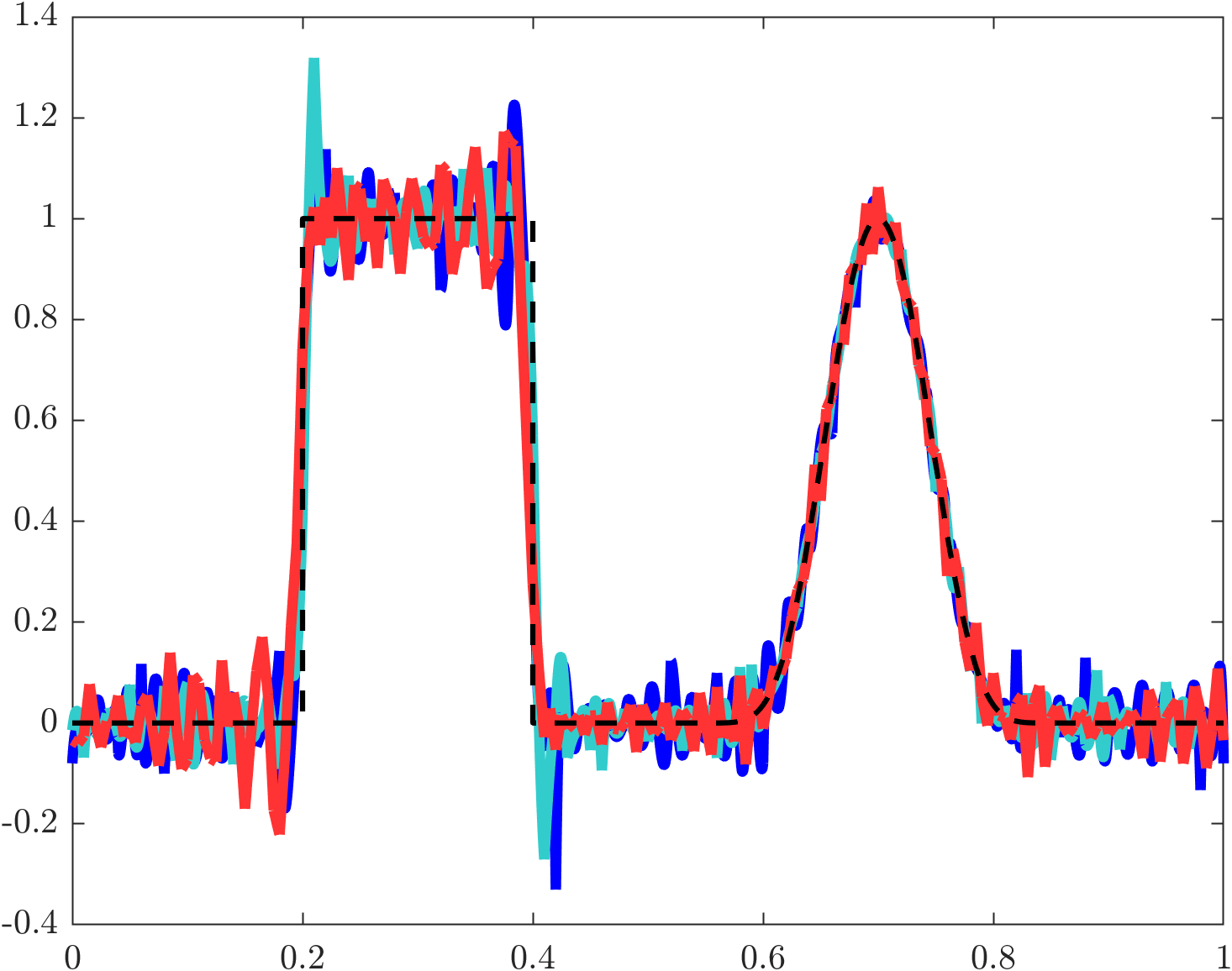
(a) CG

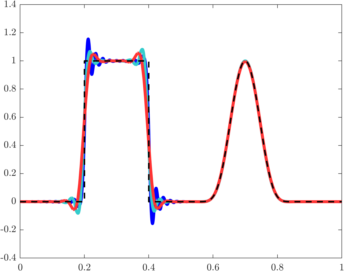
(b) HO

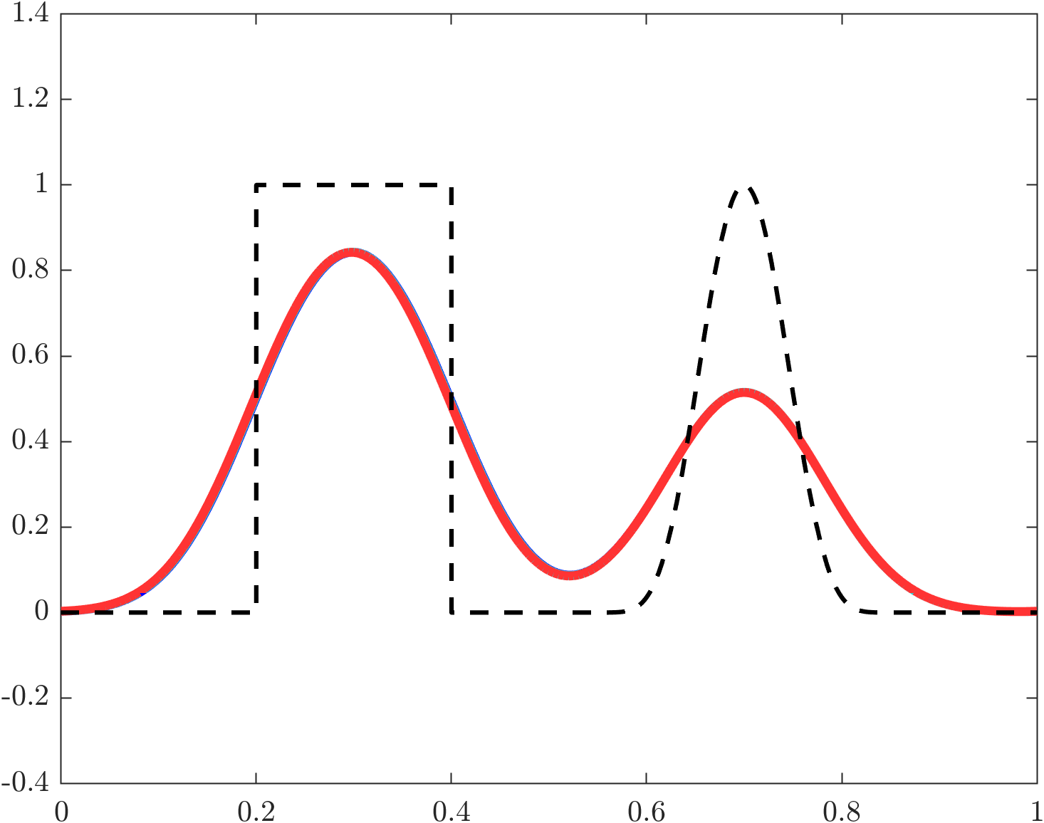
(c) LO

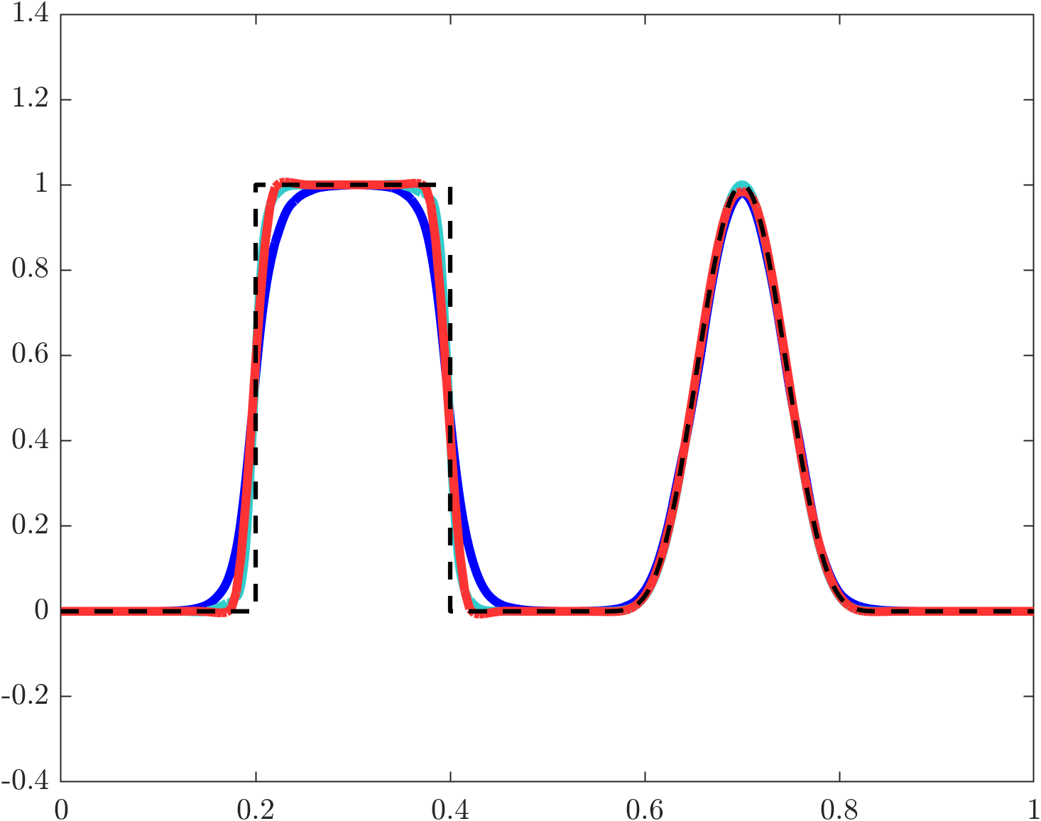
(d) WENO

Figure 1: 1D linear advection, numerical solutions at $t=1$ obtained using $N_{h}=200$ and $p=\{1,2,4\}$.

7.2 One-dimensional inviscid Burgers equation

In the next experiment, we solve the one-dimensional inviscid Burgers equation

$$\frac{\partial u}{\partial t}+\frac{\partial(u^{2}/2)}{\partial x}=0\quad\mbox{in}\ \Omega=(0,1).$$ (22)

The initial condition for this nonlinear test problem is given by

$$u_{0}(x)=\sin(2\pi x).$$ (23)

It can be shown that the unique entropy solution develops a shock at the critical time $t_{c}=\frac{1}{2\pi}$. In our grid convergence studies, we stop computations at $t=0.1<t_{c}$, because this final time is small enough for the exact solution to remain sufficiently smooth. Table 3 shows that optimal EOCs can again be achieved using HO and WENO stabilization. The $L^{1}$ convergence rate of the standard CG method is also as high as $p+1$ for odd polynomial degrees but drops down to $p$ for even ones.

	CG		VMS		WENO
$N_{h}$	$\|u_{h}-u_{\text{exact}}\|_{L^{1}}$	EOC	$\|u_{h}-u_{\text{exact}}\|_{L^{1}}$	EOC	$\|u_{h}-u_{\text{exact}}\|_{L^{1}}$	EOC
16	1.22e-2	2.13	1.19e-2	2.13	2.16e-2	2.24
32	2.56e-3	2.25	2.55e-3	2.22	5.81e-3	1.90
64	6.05e-4	2.08	6.04e-4	2.08	1.10e-3	2.40
128	1.49e-4	2.02	1.49e-4	2.02	1.56e-4	2.82
256	3.72e-5	2.00	3.72e-5	2.00	3.71e-5	2.07
512	9.29e-6	2.00	9.29e-6	2.00	9.28e-6	2.00
1024	2.33e-6	2.00	2.33e-6	2.00	2.32e-6	2.00

(a) $p=1$

	CG		VMS		WENO
$N_{h}$	$\|u_{h}-u_{\text{exact}}\|_{L^{1}}$	EOC	$\|u_{h}-u_{\text{exact}}\|_{L^{1}}$	EOC	$\|u_{h}-u_{\text{exact}}\|_{L^{1}}$	EOC
32	8.51e-4	2.99	8.07e-4	3.03	5.70e-4	3.27
64	2.73e-4	1.64	2.11e-4	1.94	1.47e-4	1.95
128	6.34e-5	2.11	3.44e-5	2.62	1.91e-5	2.94
256	1.52e-5	2.06	5.21e-6	2.72	2.33e-6	3.04
512	3.73e-6	2.02	7.68e-7	2.76	2.87e-7	3.02
1024	9.27e-7	2.01	1.10e-7	2.80	3.58e-8	3.00

(b) $p=2$

	CG		VMS		WENO
$N_{h}$	$\|u_{h}-u_{\text{exact}}\|_{L^{1}}$	EOC	$\|u_{h}-u_{\text{exact}}\|_{L^{1}}$	EOC	$\|u_{h}-u_{\text{exact}}\|_{L^{1}}$	EOC
48	3.46e-4	2.25	2.53e-4	2.17	2.29e-4	1.91
96	1.42e-5	4.60	1.15e-5	4.46	1.67e-5	3.78
192	5.35e-7	4.73	4.92e-7	4.55	1.00e-6	4.06
384	2.77e-8	4.27	2.76e-8	4.16	5.79e-8	4.11
768	1.68e-9	4.04	1.67e-9	4.04	3.49e-9	4.05
1536	1.05e-10	4.01	1.04e-10	4.01	2.15e-10	4.02

(c) $p=3$

	CG		VMS		WENO
$N_{h}$	$\|u_{h}-u_{\text{exact}}\|_{L^{1}}$	EOC	$\|u_{h}-u_{\text{exact}}\|_{L^{1}}$	EOC	$\|u_{h}-u_{\text{exact}}\|_{L^{1}}$	EOC
64	5.07e-5	3.98	3.69e-5	4.03	1.15e-4	3.78
128	9.87e-7	5.68	4.83e-7	6.26	1.55e-6	6.21
256	9.11e-8	3.44	4.25e-8	3.51	6.19e-8	4.65
512	5.47e-9	4.06	1.59e-9	4.74	1.27e-9	5.60
1024	3.32e-10	4.04	5.89e-11	4.76	3.70e-11	5.10

(d) $p=4$

Table 3: 1D Burgers equation, grid convergence history for finite elements of degree $p\in\{1,2,3,4\}$.

Extending the final time to $t=1.0>t_{c}$, we study the shock-capturing properties of the WENO scheme and its linear ingredients. Simulations are run using $p\in\{1,2,4\}$ on meshes corresponding to $N_{h}=200$ DoFs. The HO results shown in Fig. 2(a) indicate that high-order dissipation is not suited for shock capturing. The LO solutions presented in Fig. 2(b) are nonoscillatory and not as diffusive as in the case of linear advection, because shock fronts are self-steepening. Even higher resolution can be achieved using the WENO scheme, which produces the result shown in Fig. 2(c). Remarkably, the LO and WENO approximations remain virtually unchanged as we vary $p$ while keeping $N_{h}$ fixed. The differences between the oscillatory HO results for different polynomial degrees are clearly visible.

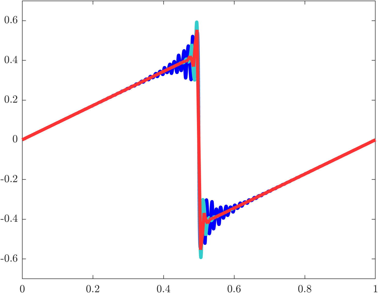
(a) HO

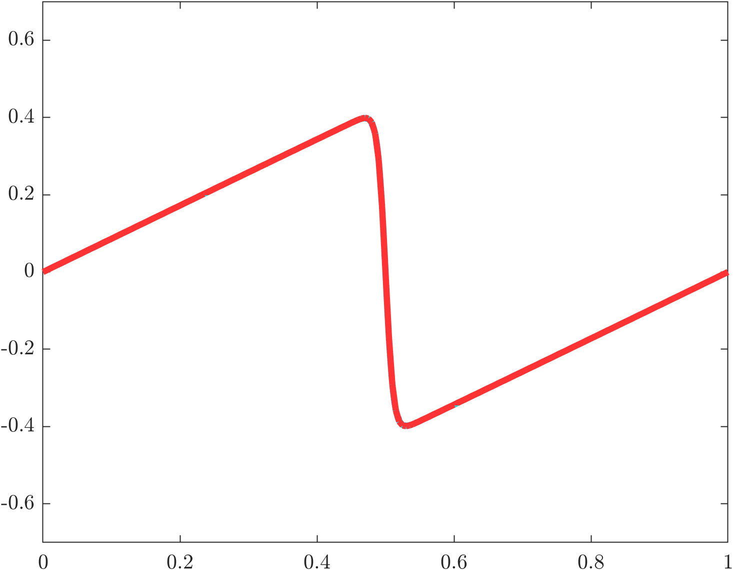
(b) LO

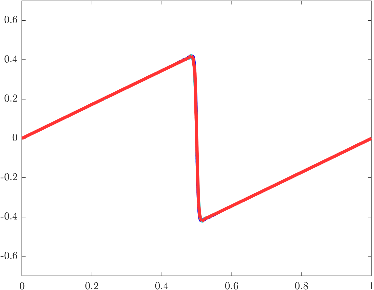
(c) WENO

Figure 2: 1D Burgers equation, numerical solutions at $t=1.0$ obtained using $N_{h}=200$ and $p=\{1,2,4\}$.

7.3 Two-dimensional solid body rotation

LeVeque’s [32] solid body rotation problem is a popular stability test for discretizations of

$$\frac{\partial u}{\partial t}+\nabla\cdot(\mathbf{v}u)=0\quad\mbox{in}\ \Omega=(0,1)^{2}.$$ (24)

The velocity field ${\bf v}(x,y)=2\pi(0.5-y,x-0.5)$ is divergence-free. The initial condition is given by

$$u_{0}(x,y)=\begin{cases}u_{0}^{\text{hump}}(x,y)&\mbox{if}\ \sqrt{(x-0.25)^{2}+(y-0.5)^{2}}\leq 0.15,\\ u_{0}^{\text{cone}}(x,y)&\mbox{if}\ \sqrt{(x-0.5)^{2}+(y-0.25)^{2}}\leq 0.15,\\ 1&\mbox{if}\;\begin{cases}\sqrt{(x-0.5)^{2}+(y-0.75)^{2}}\leq 0.15,\\ |x-0.5|\geq 0.025,y\geq 0.85,\end{cases}\\ 0&\mbox{otherwise},\end{cases}$$ (25)

where

$$u_{0}^{\text{hump}}(x,y) =\frac{1}{4}+\frac{1}{4}\cos\bigg{(}\frac{\pi\sqrt{(x-0.25)^{2}+(y-0.5)^{2}}}{0.15}\bigg{)},$$

$$u_{0}^{\text{cone}}(x,y) =1-\frac{\sqrt{(x-0.5)^{2}+(y-0.25)^{2}}}{0.15}.$$

The initial configuration rotates around the center $(0.5,0.5)$ of $\Omega$. After each complete revolution (i.e., for $t\in\mathbb{N}$), the exact solution of the linear advection equation (22) coincides with $u_{0}$.

We evolve numerical solutions up to the finite time $t=1.0$ on uniform Cartesian meshes corresponding to $N_{h}=129^{2}$ DoFs. The results for Lagrange finite elements of degree $p=\{1,2,4\}$ are presented in Figs 3–5. All CG approximations are corrupted by global spurious oscillations. The HO stabilization is sufficient in smooth regions but large undershoots and overshoots are observed in the vicinity of the slotted cylinder. The LO solution is nonoscillatory but very diffusive. Using the smoothness indicator $\gamma_{e}$ to adaptively blend HO and LO dissipation, the nonlinear WENO scheme exploits the complementary advantages of the two linear methods and yields superior results for all combinations of the mesh size $h$ and polynomial degree $p$. To show that $h$ is coarsened as $p$ is refined to keep $N_{h}$ fixed, we plot the edges of the meshes on which the computations were performed.

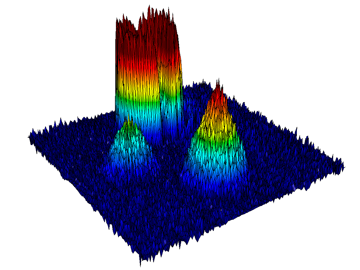
(a) CG, $E_{1}$=3.70e-02, $u_{h}\in[-0.399,1.367]$

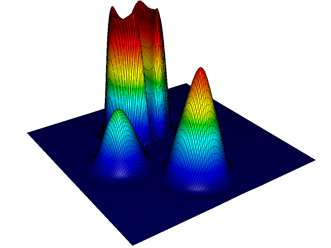
(b) HO, $E_{1}$=1.47e-02, $u_{h}\in[-0.055,1.122]$

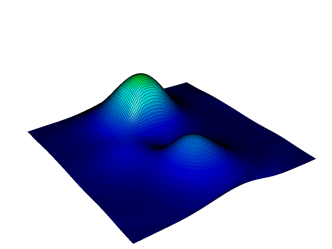
(c) LO, $E_{1}$=1.10e-01, $u_{h}\in[0.003,0.478]$

(d) WENO, $E_{1}$=2.68e-02, $u_{h}\in[-0.001,0.993]$

Figure 3: Solid body rotation, numerical solutions at $t=1$ obtained using $N_{h}=129^{2}$ and $p=1$.

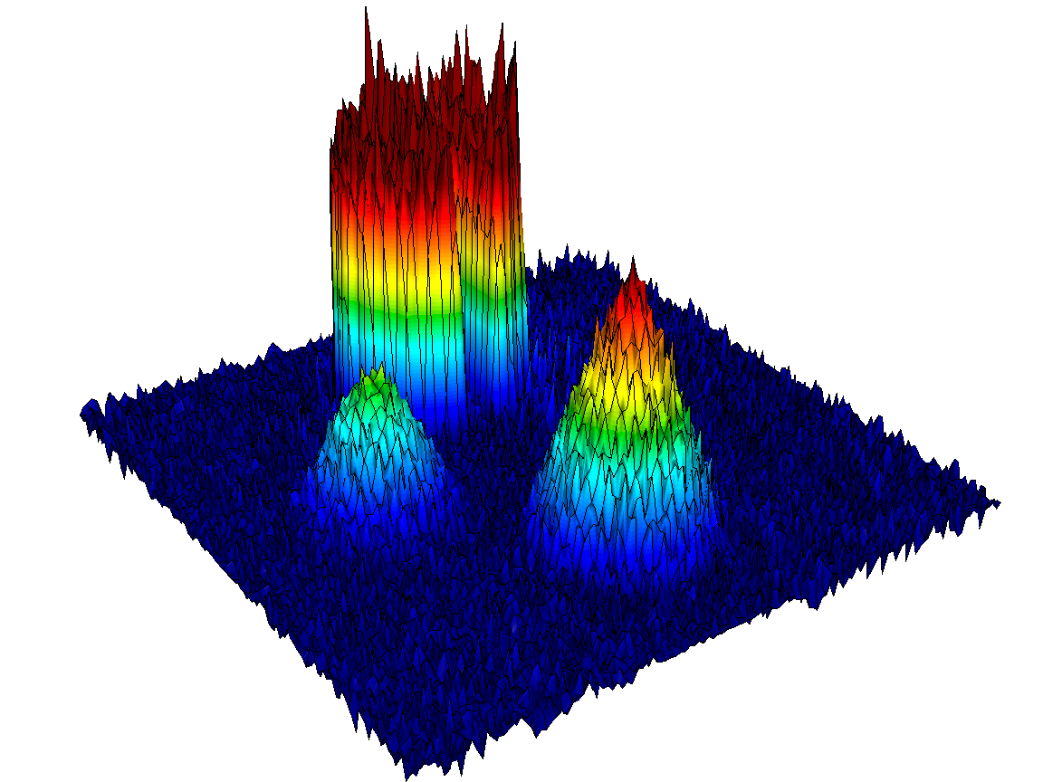
(a) CG, $E_{1}$=3.17e-02, $u_{h}\in[-0.377,1.476]$

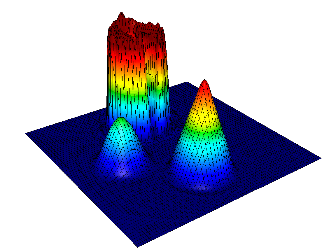
(b) HO, $E_{1}$=1.23e-02, $u_{h}\in[-0.213,1.183]$

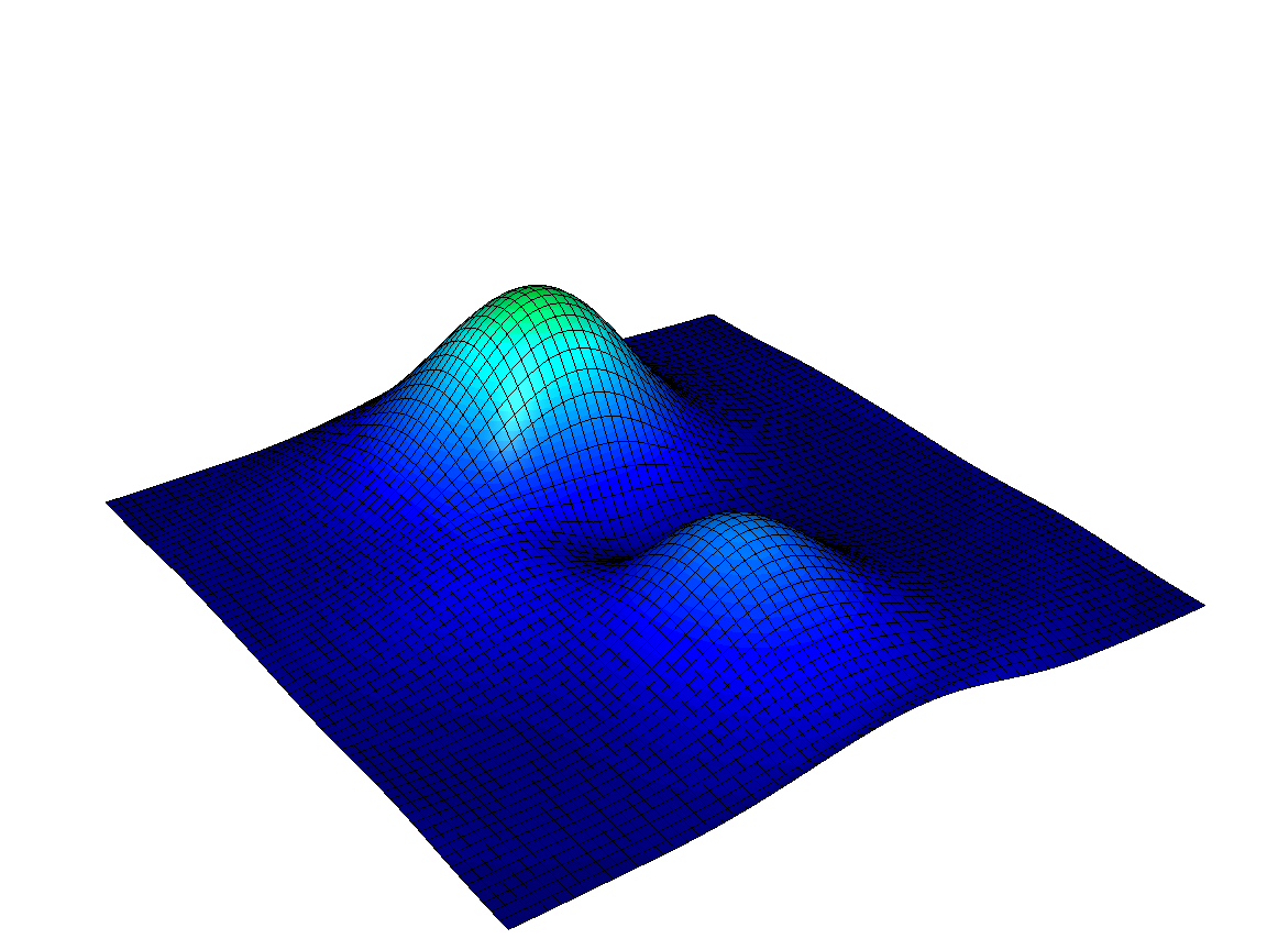
(c) LO, $E_{1}$=1.10e-01, $u_{h}\in[0.004,0.465]$

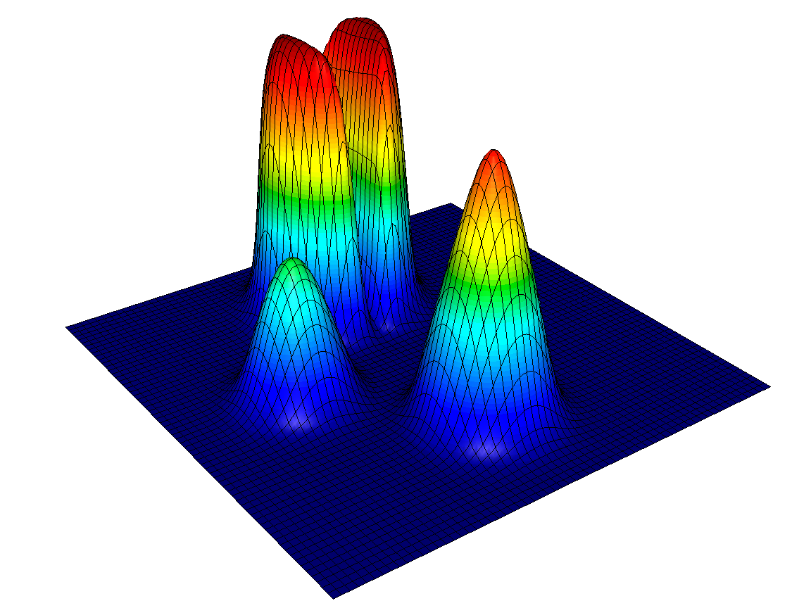
(d) WENO, $E_{1}$=2.67e-01, $u_{h}\in[0.000,0.981]$

Figure 4: Solid body rotation, numerical solutions at $t=1$ obtained using $N_{h}=129^{2}$ and $p=2$.

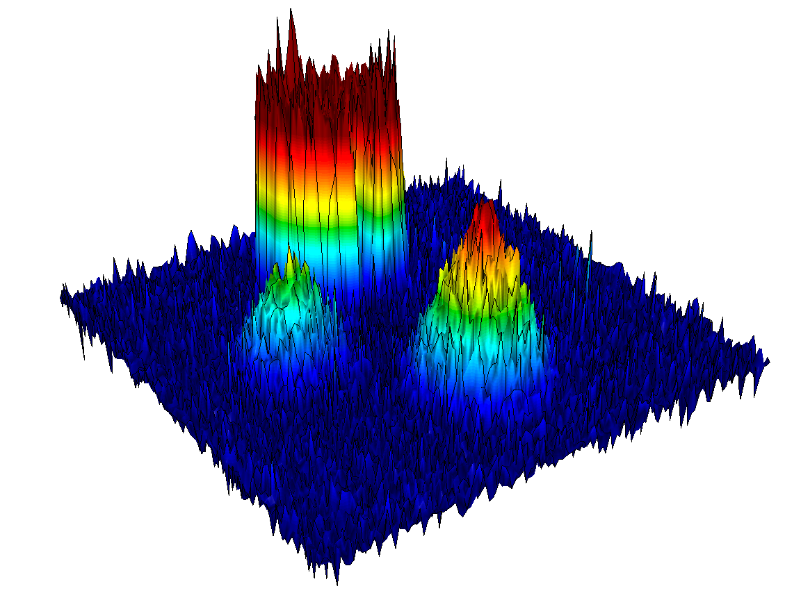
(a) CG, $E_{1}$=4.19e-02, $u_{h}\in[-0.480,1.429]$

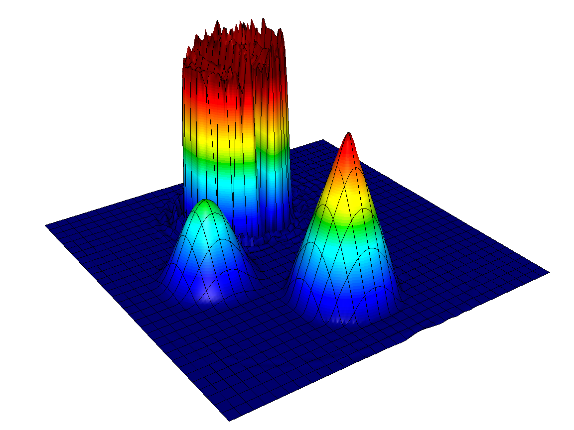
(b) HO, $E_{1}$=1.25e-02, $u_{h}\in[-0.265,1.266]$

(c) LO, $E_{1}$=1.11e-01, $u_{h}\in[0.004,0.501]$

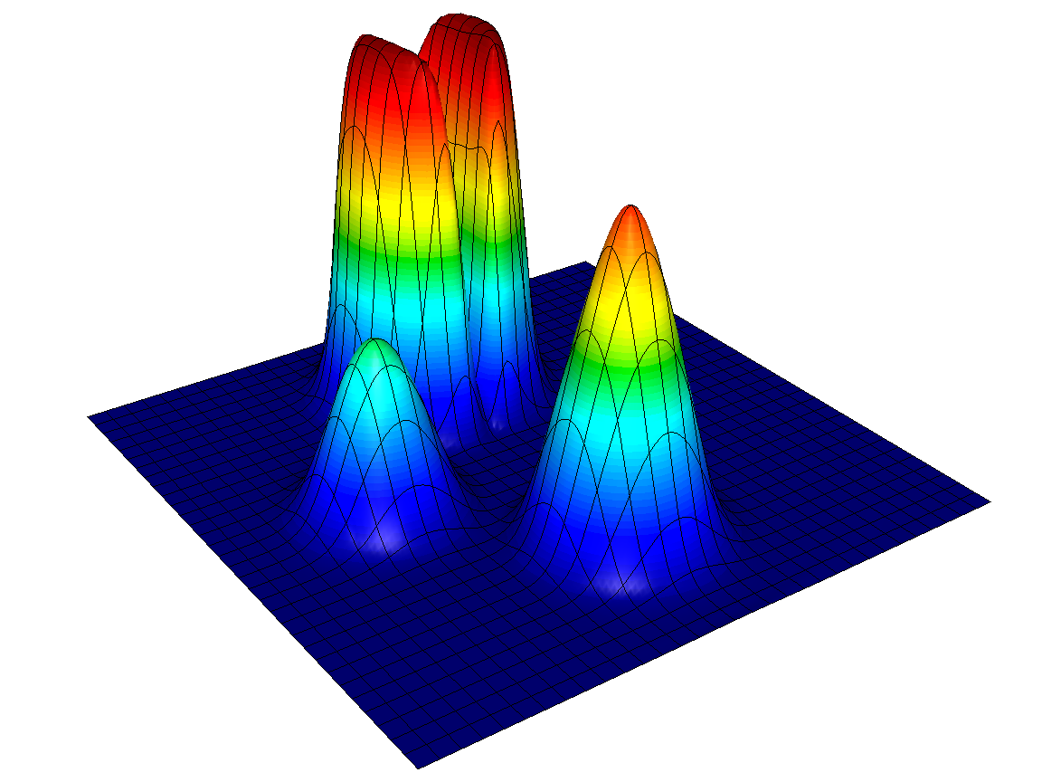
(d) WENO, $E_{1}$=2.76e-02, $u_{h}\in[0.000,0.998]$

Figure 5: Solid body rotation, numerical solutions at $t=1$ obtained using $N_{h}=129^{2}$ and $p=4$.

7.4 KPP problem

Finally, we consider the KPP problem [26, 31], a challenging nonlinear test for assessment of entropy stability properties. The conservation law (1a) with the nonconvex flux function

$$\mathbf{f}(u)=(\sin(u),\cos(u))$$ (26)

is solved in the computational domain $\Omega_{h}=(-2,2)\times(-2.5,1.5)$ using the initial condition

$$u_{0}(x,y)=\begin{cases}\frac{7\pi}{2}&\mbox{if}\quad\sqrt{x^{2}+y^{2}}\leq 1,\\ \frac{\pi}{4}&\mbox{otherwise}.\end{cases}$$ (27)

A global upper bound for the maximum speed that we need to calculate the viscosity parameter $\nu_{e}$ is given by $\lambda_{e}=1$. To make the LO component of the WENO scheme as dissipative as necessary to safely suppress undershoots/overshoots even on coarsest meshes, we define it using $\lambda_{e}=2$. Deviating from the default settings, we choose the linear weights $\tilde{\omega}_{l}^{e}=0.2,\ l=0,\ldots,4$. As mentioned above, smaller values of $\tilde{\omega}_{0}^{e}$ make the smoothness indicator $\gamma_{e}$ more sensitive to spurious oscillations. Finally, we lump the mass matrix in the CG version without any stabilization ($\nu_{e}=0$) because the consistent-mass CG approximation was found to produce extremely oscillatory results in this test.

As in the previous example, we run simulations on uniform meshes of square cells corresponding to $N_{h}=129^{2}$ DoFs. The numerical results for $p=\{1,2,4\}$ are displayed in Figs 6–8. The lumped-mass CG method produces strong oscillations and an entropy-violating shock. The HO stabilization alleviates the former problem (to some extent) but not the lack of entropy stability. The LO results and the less diffusive WENO solutions are nonoscillatory. Moreover, they reproduce the spiral wave structure of the entropy solution to the two-dimensional Riemann problem. The small undershoot in the WENO result for $p=4$ is due to the use of a cell-based smoothness indicator on a coarse mesh. Such undershoots/overshoots disappear as the mesh is refined. If necessary, preservation of global bounds and validity of entropy inequalities can be strictly enforced using the algebraic flux correction tools presented in [29, 31]. In fact, the development of our WENO scheme was largely motivated by the possibility of using it as a baseline discretization for flux limiting approaches that perform accuracy-preserving local fixes to enforce physical admissibility conditions (cf. [28, 47, 49]).

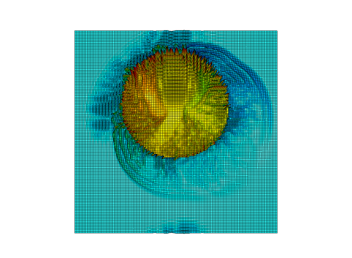
(a) CG, $u_{h}\in[-11.752,24.446]$

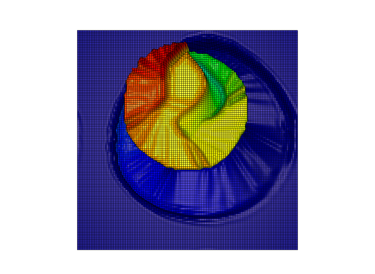
(b) HO, $u_{h}\in[-2.986,15.271]$

(c) LO, $u_{h}\in[0.785,10.893]$

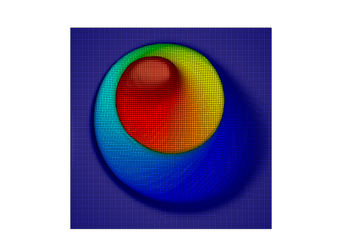
(d) WENO, $u_{h}\in[0.785,10.990]$

Figure 6: KPP problem, numerical solutions at $t=1$ obtained using $N_{h}=129^{2}$ and $p=1$.

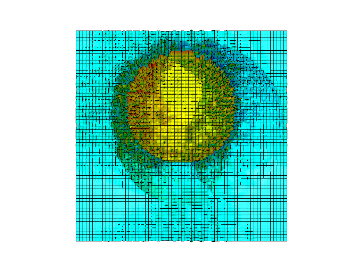
(a) CG, $u_{h}\in[-16.934,29.237]$

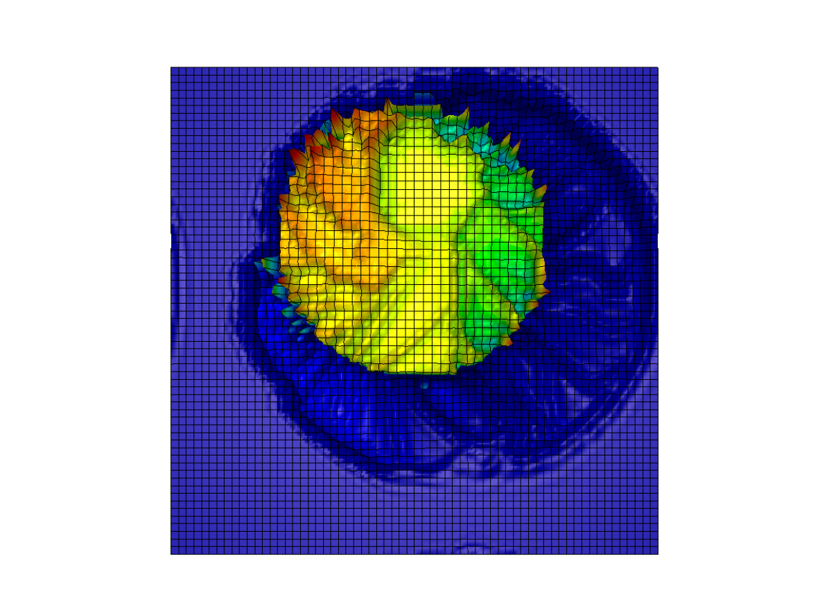
(b) HO, $u_{h}\in[-8.503,19.027]$

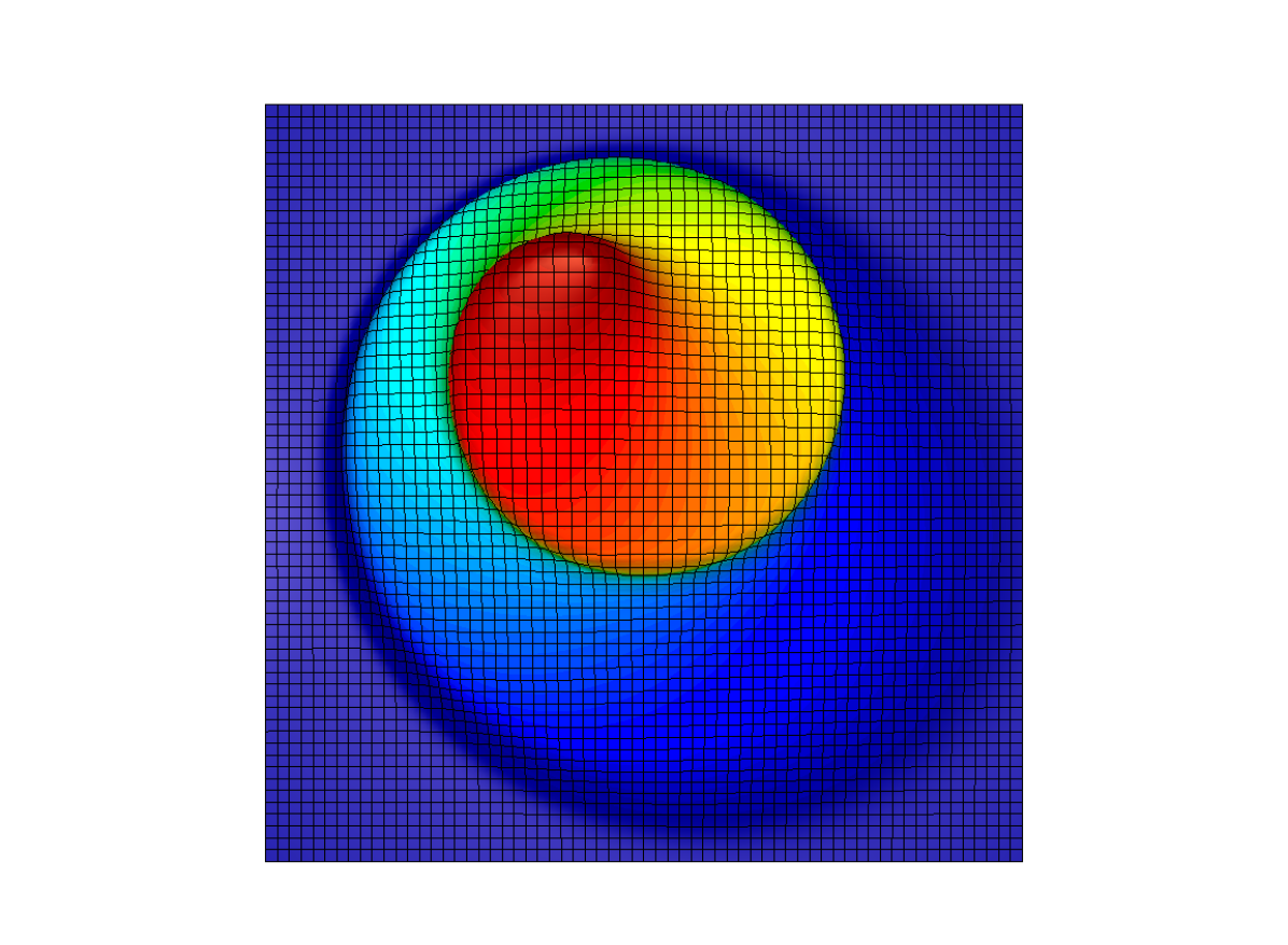
(c) LO, $u_{h}\in[0.785,10.885]$

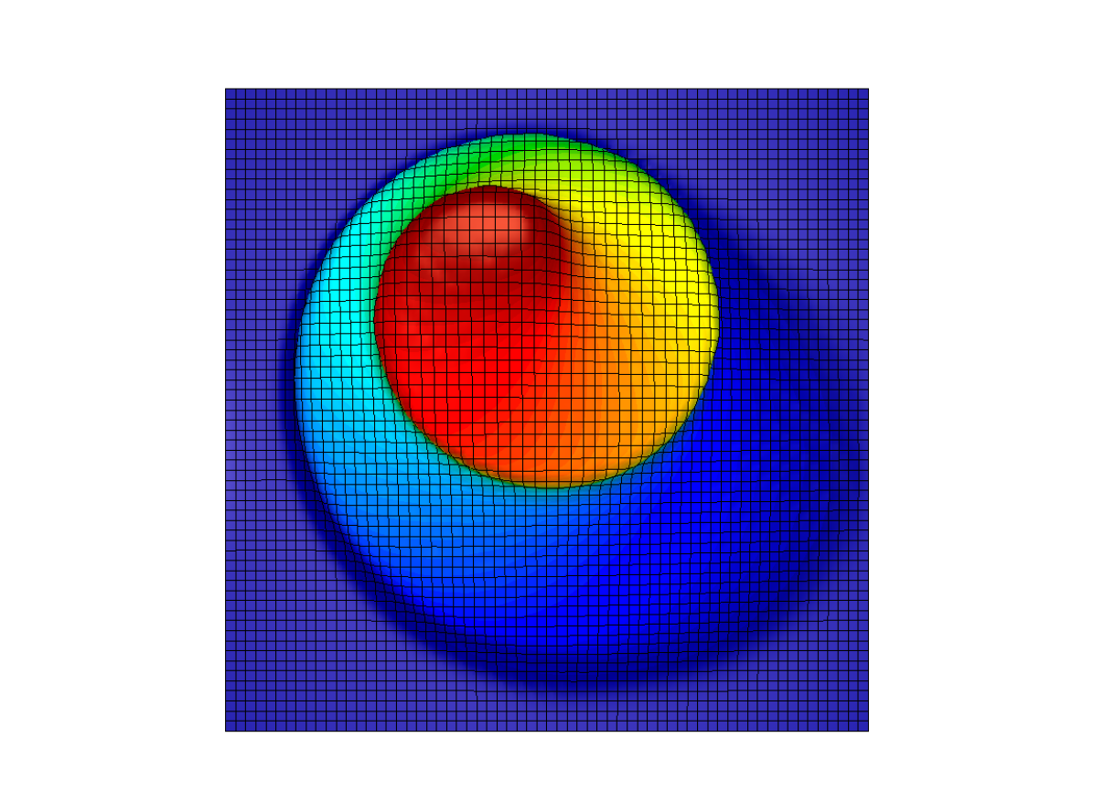
(d) WENO, $u_{h}\in[0.785,10.983]$

Figure 7: KPP problem, numerical solutions at $t=1$ obtained using $N_{h}=129^{2}$ and $p=2$.

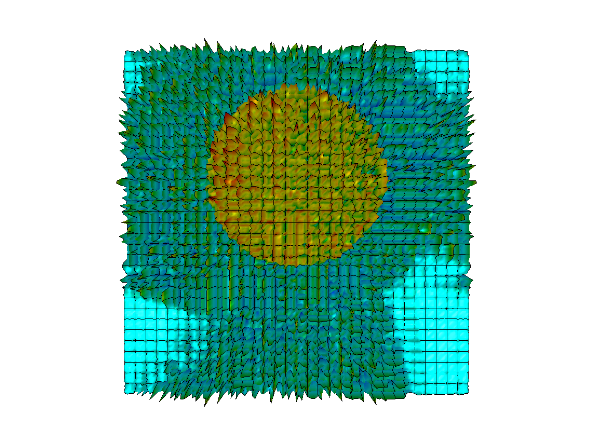
(a) CG, $u_{h}\in[-16.260,28.369]$

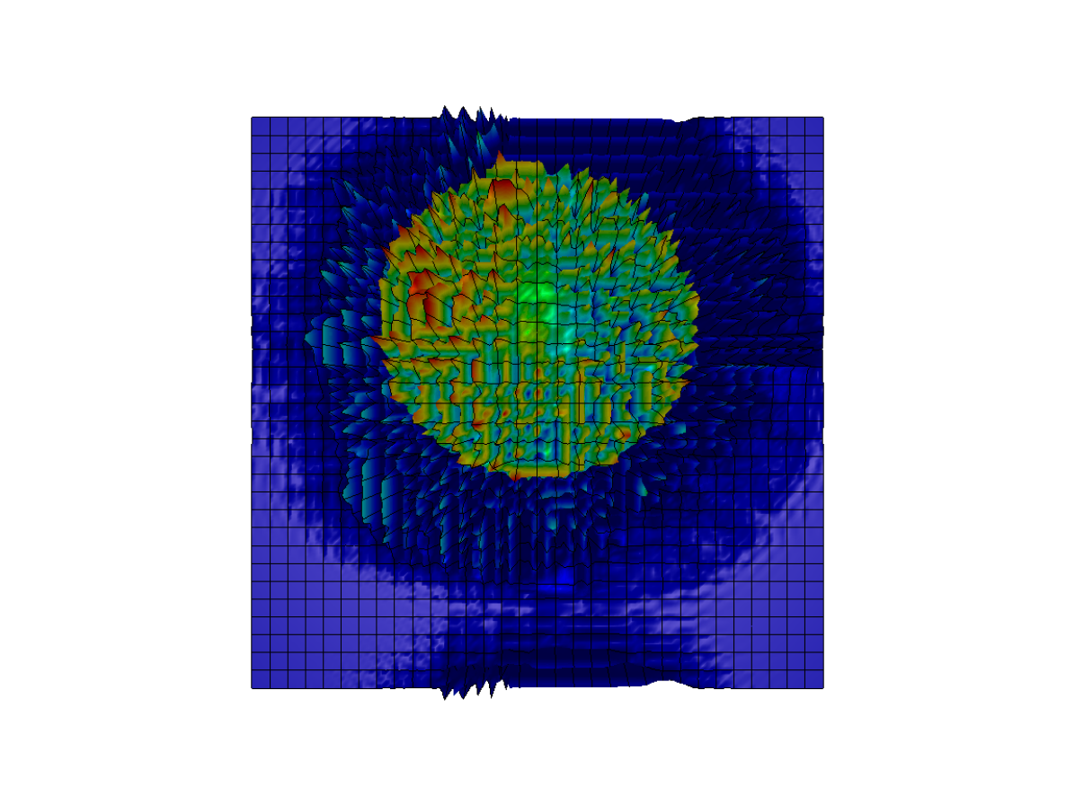
(b) HO, $u_{h}\in[-10.828,22.094]$

(c) LO, $u_{h}\in[0.785,10.882]$

(d) WENO, $u_{h}\in[0.778,10.980]$

Figure 8: KPP problem, numerical solutions at $t=1$ obtained using $N_{h}=129^{2}$ and $p=4$.

8 Conclusions

We discussed a new way to combine high- and low-order components of dissipation-based stabilization operators for CG discretizations of hyperbolic conservation laws. Using piecewise-constant blending functions that measure deviations from a WENO reconstruction, we managed to achieve optimal convergence rates while avoiding spurious oscillations both globally and locally. The resulting hybrid scheme has the structure of a nonlinear artificial diffusion method. Therefore, it is easier to analyze than DG-WENO schemes in which partial derivatives of approximate solutions are manipulated directly. Our theoretical investigations provide an optimal estimate for the consistency error of the nonlinear stabilization and worst-case a priori error estimates for steady advection-reaction equations. The modular design makes it easy to upgrade individual building blocks (stabilization operators, smoothness indicators, reconstruction procedures) of the presented algorithm step-by-step. In particular, it is worthwhile to investigate if the accuracy of CG-WENO schemes can be improved by using Lagrange interpolation polynomials (as in [36]), additional stencils for Hermite interpolation, and/or alternative definitions of the linear weights. Another promising avenue for further research is the use of dissipation-based WENO stabilization in the DG context. Last but not least, the cost of calculating smoothness indicators needs to be reduced, e.g., by using troubled cell detectors as in [51, 53].

Acknowledgments

This article is dedicated to the memory of Prof. Roland Glowinski, a great mathematician who provided guidance and support to the first author many times over a span of two decades. Roland’s wisdom and kindness will always be remembered.

The development of the proposed methodology was sponsored by the German Research Association (Deutsche Forschungsgemeinschaft, DFG) under grant KU 1530/23-3.

References

- [1] Rémi Abgrall. On essentially non-oscillatory schemes on unstructured meshes: Analysis and implementation. J. Comput. Phys., 114(1):45–58, 1994.
- [2] Rémi Abgrall. Essentially non-oscillatory residual distribution schemes for hyperbolic problems. J. Comput. Phys., 214(2):773–808, 2006.
- [3] Robert Anderson, Julian Andrej, Andrew Barker, Jamie Bramwell, Jean-Sylvain Camier, Jakub Cerveny, Veselin Dobrev, Yohann Dudouit, Aaron Fisher, Tzanio Kolev, Will Pazner, Mark Stowell, Vladimir Tomov, Ido Akkerman, Johann Dahm, David Medina, and Stefano Zampini. MFEM: a Modular Finite Element Methods Library. Comput. Math. Appl., 81:42–74, 2021.
- [4] Santiago Badia and Alba Hierro. On monotonicity-preserving stabilized finite element approximations of transport problems. SIAM J. Sci. Comput., 36(6):A2673–A2697, 2014.
- [5] Gabriel R. Barrenechea, Erik Burman, and Fotini Karakatsani. Blending low-order stabilised finite element methods: A positivity-preserving local projection method for the convection–diffusion equation. Computer Methods Appl. Meth. Engrg., 317:1169–1193, 2017.
- [6] Gabriel R. Barrenechea, Erik Burman, and Fotini Karakatsani. Edge-based nonlinear diffusion for finite element approximations of convection–diffusion equations and its relation to algebraic flux-correction schemes. Numer. Math., 135(2):521–545, 2017.
- [7] Gabriel R. Barrenechea, Volker John, and Petr Knobloch. Analysis of algebraic flux correction schemes. SIAM J. Numer. Anal., 54(4):2427–2451, 2016.
- [8] Gabriel R. Barrenechea, Volker John, Petr Knobloch, and Richard Rankin. A unified analysis of algebraic flux correction schemes for convection-diffusion equations. SeMA J., 75(4):655–685, 2018.
- [9] Malte Braack and Erik Burman. Local projection stabilization for the Oseen problem and its interpretation as a variational multiscale method. SIAM J. Numer. Anal., 43(6):2544–2566, 2006.
- [10] Alexander N. Brooks and Thomas J. R. Hughes. Streamline upwind/Petrov–Galerkin formulations for convection dominated flows with particular emphasis on the incompressible Navier–Stokes equations. Computer Methods Appl. Meth. Engrg., 32(1-3):199–259, 1982.
- [11] Erik Burman. Consistent SUPG-method for transient transport problems: Stability and convergence. Computer Methods Appl. Meth. Engrg., 199(17):1114–1123, 2010.
- [12] Erik Burman and Alexandre Ern. Implicit-explicit Runge–Kutta schemes and finite elements with symmetric stabilization for advection-diffusion equations. ESAIM:M2AN, 46(4):681–707, 2012.
- [13] Veselin Dobrev, Tzanio Kolev, Dmitri Kuzmin, Robert Rieben, and Vladimir Tomov. Sequential limiting in continuous and discontinuous Galerkin methods for the Euler equations. J. Comput. Phys., 356:372–390, 2018.
- [14] Jean Donea and Antonio Huerta. Finite Element Methods for Flow Problems. John Wiley & Sons, Chichester, 2003.
- [15] Oliver Friedrich. Weighted essentially non-oscillatory schemes for the interpolation of mean values on unstructured grids. J. Comput. Phys., 144(1):194–212, 1998.
- [16] Sigal Gottlieb, Chi-Wang Shu, and Eitan Tadmor. Strong stability-preserving high-order time discretization methods. SIAM Rev., 43(1):89–112, 2001.
- [17] Hennes Hajduk. Monolithic convex limiting in discontinuous Galerkin discretizations of hyperbolic conservation laws. Comput. Math. Appl., 87:120–138, 2021.
- [18] Hennes Hajduk, Dmitri Kuzmin, Tzanio Kolev, Vladimir Tomov, Ignacio Tomas, and John N Shadid. Matrix-free subcell residual distribution for Bernstein finite elements: Monolithic limiting. Comput. Fluids, 200:104451, 2020.
- [19] Ami Harten, Bjorn Engquist, Stanley Osher, and Sukumar R Chakravarthy. Uniformly high order accurate essentially non-oscillatory schemes, III. J. Comput. Phys., 71(2):231–303, 1987.
- [20] Ralf Hartmann. Numerical analysis of higher order discontinuous Galerkin finite element methods, 2008. Lecture notes, DLR (German Aerospace Center).
- [21] Antony Jameson. Origins and further development of the Jameson–Schmidt–Turkel scheme. AIAAJournal, 55(5):1487–1510, 2017.
- [22] Antony Jameson, Wolfgang Schmidt, and Eli Turkel. Numerical solution of the Euler equations by finite volume methods using Runge–Kutta time stepping schemes. AIAA Paper 81-1259, 1981.
- [23] Guang Shan Jiang and Chi-Wang Shu. Efficient implementation of Weighted ENO schemes. J. Comput. Phys., 126(1):202–228, 1996.
- [24] Volker John, Songul Kaya, and William Layton. A two-level variational multiscale method for convection-dominated convection-diffusion equations. Computer Methods Appl. Meth. Engrg., 195(33):4594–4603, 2006.
- [25] Lilia Krivodonova, Jianguo Xin, Jean-François Remacle, Nicolas Chevaugeon, and Joseph E. Flaherty. Shock detection and limiting with discontinuous Galerkin methods for hyperbolic conservation laws. Appl. Numer. Math., 48(3–4):323–338, 2004.
- [26] Alexander Kurganov, Guergana Petrova, and Bojan Popov. Adaptive semidiscrete central-upwind schemes for nonconvex hyperbolic conservation laws. SIAM J. Sci. Comput., 29(6):2381–2401, 2007.
- [27] Dmitri Kuzmin. Algebraic flux correction I. Scalar conservation laws. In Dmitri Kuzmin, Rainald Löhner, and Stefan Turek, editors, Flux-Corrected Transport: Principles, Algorithms, and Applications, pages 145–192. Springer, 2 edition, 2012.
- [28] Dmitri Kuzmin and Hennes Hajduk. Property-Preserving Numerical Schemes for Conservation Laws. World Scientific, 2023, to appear.
- [29] Dmitri Kuzmin, Hennes Hajduk, and Andreas Rupp. Limiter-based entropy stabilization of semi-discrete and fully discrete schemes for nonlinear hyperbolic problems. Computer Methods Appl. Meth. Engrg., 389:114428, 2022.
- [30] Dmitri Kuzmin and Nikita Klyushnev. Limiting and divergence cleaning for continuous finite element discretizations of the MHD equations. J. Comput. Phys., 407:109230, 2020.
- [31] Dmitri Kuzmin and Manuel Quezada de Luna. Entropy conservation property and entropy stabilization of high-order continuous Galerkin approximations to scalar conservation laws. Comput. Fluids, 213:104742, 2020.
- [32] Randall J LeVeque. High-resolution conservative algorithms for advection in incompressible flow. SIAM J. Numer. Anal., 33(2):627–665, 1996.
- [33] Xu-Dong Liu, Stanley Osher, and Tony Chan. Weighted essentially non-oscillatory schemes. J. Comput. Phys., 115(1):200–212, 1994.
- [34] Christoph Lohmann. Physics-Compatible Finite Element Methods for Scalar and Tensorial Advection Problems. Springer Spektrum, 2019.
- [35] Christoph Lohmann, Dmitri Kuzmin, John N. Shadid, and Sibusiso Mabuza. Flux-corrected transport algorithms for continuous Galerkin methods based on high order Bernstein finite elements. J. Comput. Phys., 344:151–186, 2017.
- [36] Hong Luo, Joseph D. Baum, and Rainald Löhner. A Hermite WENO-based limiter for discontinuous Galerkin method on unstructured grids. J. Comput. Phys., 225(1):686–713, 2007.
- [37] Hong Luo, Joseph D. Baum, and Rainald Löhner. A discontinuous Galerkin method based on a Taylor basis for the compressible flows on arbitrary grids. J. Comput. Phys., 227(20):8875–8893, 2008.
- [38] Hong Luo, Yidong Xia, Shujie Li, Robert Nourgaliev, and Chunpei Cai. A Hermite WENO reconstruction-based discontinuous Galerkin method for the Euler equations on tetrahedral grids. J. Comput. Phys., 231(16):5489–5503, 2012.
- [39] MFEM: a Modular Finite Element Methods library [web site]. https://mfem.org.
- [40] Per-Olof Persson and Jaime Peraire. Sub-cell shock capturing for discontinuous Galerkin methods. In 44th AIAA Aerospace Sciences Meeting and Exhibit, page 112, 2006.
- [41] Jianxian Qiu and Chi-Wang Shu. Runge–Kutta discontinuous Galerkin method using weno limiters. SIAM J. Sci. Comput., 26(3):907–929, 2005.
- [42] Alfio Quarteroni and Alberto Valli. Numerical Approximation of Partial Differential Equations. Springer, 1994.
- [43] Vittorio Selmin. The node-centred finite volume approach: Bridge between finite differences and finite elements. Comput. Methods Appl. Mech. Engrg., 102(1):107–138, 1993.
- [44] Chi-Wang Shu. Essentially non-oscillatory and weighted essentially non-oscillatory schemes for hyperbolic conservation laws. In Advanced Numerical Approximation of Nonlinear Hyperbolic Equations, Lecture Notes in Mathematics, pages 325–432. Springer, 1998.
- [45] Chi-Wang Shu. High order weighted essentially nonoscillatory schemes for convection dominated problems. SIAM Rev., 51(1):82–126, 2009.
- [46] Chi-Wang Shu. High order WENO and DG methods for time-dependent convection-dominated PDEs: A brief survey of several recent developments. J. Comput. Phys., 316:598–613, 2016.
- [47] Xiangxiong Zhang and Chi-Wang Shu. On maximum-principle-satisfying high order schemes for scalar conservation laws. J. Comput. Phys., 229(9):3091–3120, 2010.
- [48] Xiangxiong Zhang and Chi-Wang Shu. On positivity-preserving high order discontinuous Galerkin schemes for compressible Euler equations on rectangular meshes. J. Comput. Phys., 229(23):8918–8934, 2010.
- [49] Xiangxiong Zhang and Chi-Wang Shu. Maximum-principle-satisfying and positivity-preserving high-order schemes for conservation laws: Survey and new developments. Proc. R. Soc. A, 467(2134):2752–2776, 2011.
- [50] Xiangxiong Zhang, Yinhua Xia, and Chi-Wang Shu. Maximum-principle-satisfying and positivity-preserving high order discontinuous Galerkin schemes for conservation laws on triangular meshes. J. Sci. Comput., 50(1):29–62, 2012.
- [51] Xinghui Zhong and Chi-Wang Shu. A simple weighted essentially nonoscillatory limiter for Runge–Kutta discontinuous Galerkin methods. J. Comput. Phys., 232(1):397–415, 2013.
- [52] Jun Zhu and Jianxian Qiu. Hermite WENO schemes and their application as limiters for Runge–Kutta discontinuous Galerkin method, III: Unstructured meshes. J. Sci. Comput., 39(2):293–321, 2009.
- [53] Jun Zhu, Xinghui Zhong, Chi-Wang Shu, and Jianxian Qiu. Runge–Kutta discontinuous Galerkin method with a simple and compact Hermite WENO limiter. Commun. Comput. Phys., 19(4):944–969, 2016.
- [54] Jun Zhu, Xinghui Zhong, Chi-Wang Shu, and Jianxian Qiu. Runge–Kutta discontinuous Galerkin method with a simple and compact Hermite WENO limiter on unstructured meshes. Commun. Comput. Phys., 21(3):623–649, 2017.