The flavor transition process $b\rightarrow s\gamma$ in the $U(1)_{X}$SSM with the mass insertion approximation

Abstract

People extend the MSSM with the local gauge group $U(1)_{X}$ to obtain the $U(1)_{X}$SSM. In the framework of the $U(1)_{X}$SSM, we study the flavor transition process $b\rightarrow{s\gamma}$ with the mass insertion approximation (MIA). By the MIA method and some reasonable parameter assumptions, we can intuitively find the parameters that have obvious effect on the analytic results of the flavor transition process $b\rightarrow{s\gamma}$. By means of the influences of different sensitive parameters, we can obtain reasonable results to better fit the experimental data.

I Introduction

The rare decay $\bar{B}\to X_{s}\gamma$ is the Flavor Changing Neutral Current (FCNC) process with great research value, whose CP averaged branching ratio is used to constrain many models of new physics. People have conducted multi-angle research on the process. The authors of Refs. bsy1 ; bsy2 ; bsy3 present the calculation of the rate of the inclusive decay $\bar{B}\to X_{s}\gamma$ in the two-Higgs doublet model (THDM). The supersymmetric effect on $\bar{B}\to X_{s}\gamma$ is discussed in Refs. bsy4 ; bsy5 ; bsy6 ; bsy7 ; bsy8 ; bsy9 .

Since the influence of new physics on FCNC process is mainly derived from the loop diagrams process, the decay process $b\to s\gamma$ is very sensitive to new physics beyond the Standard Model (SM). The average experimental data on the branching ratio of the inclusive $\bar{B}\rightarrow X_{s}\gamma$ is Average

$$BR(\bar{B}\rightarrow X_{s}\gamma)_{exp}=(3.40\pm 0.21)\times 10^{-4},$$ (1)

and the prediction of SM at next-next-to-leading order (NNLO) is SM1 ; SM2 ; SM3 ; SM4 ; SM5 ; SM6 ; SM7 ; SM8

$$BR(\bar{B}\rightarrow X_{s}\gamma)_{SM}=(3.36\pm 0.23)\times 10^{-4}.$$ (2)

A famous extension of the SM is the minimal supersymmetric extension of the standard model (MSSM) MSSM . As a popular extension, the MSSM solves many problems. However, the explanation of neutrino oscillation requires tiny neutrino mass, which can not be naturally generated by the MSSM. So people extend the MSSM into multiple models, among which, the $U(1)_{X}$ extension of the MSSM is called as the $U(1)_{X}$SSM UX2 ; UX3 with the local gauge group $SU(3)_{C}\otimes SU(2)_{L}\otimes U(1)_{Y}\otimes U(1)_{X}$. Compared to the MSSM, the $U(1)_{X}$SSM has more superfields such as right-handed neutrinos. The right-handed neutrinos and the added Higgs singlets can explain the tiny mass of neutrino. It can alleviate the $\mu$ problem of the MSSM, because $\mu\hat{H}_{u}\hat{H}_{d}$ and $\lambda_{H}\hat{S}\hat{H}_{u}\hat{H}_{d}$ in the $U(1)_{X}$SSM produce the effective $\mu_{H}^{\prime}=\mu+\lambda_{H}v_{S}/\sqrt{2}$. Mixing the CP-even parts of $H_{d},~{}H_{u},~{}\eta,~{}\bar{\eta},~{}S$ can improve the masses of the tree-level lightest and sub-lightest CP-even Higgs particles.

The mass eigenstate basis is the most commonly used method in FCNC research. However, the mass eigenstate method depends on the mass eigenvalues of particles and rotation matrices, which makes it difficult to find the sensitive parameters clearly and intuitively. To solve this problem, we use another method - Mass Insertion Approximation (MIA) UX3 ; MIA4 ; MIA1 ; MIA2 ; MIA3 . The MIA results can be alternatively obtained from expanding properly the expressions in the mass eigensate basis MEN . At the analytical level, it avoids tedious calculations and reduces the chances of errors. In addition, its relatively concise and clear analytical results are helpful for the analysis of sensitive parameters.

To sum up, we investigate the FCNC process $b\rightarrow s\gamma$ under the $U(1)_{X}$SSM by MIA. Our paper is organized as follows. In Sec.II, we mainly introduce the $U(1)_{X}$SSM including its superpotential and the general soft breaking terms. The analytic expressions for $b\rightarrow s\gamma$ decay in the $U(1)_{X}$SSM are given in Sec.III. In Sec.IV, we give the numerical analysis. And our conclusions are summarized in Sec.V.

II The $U(1)_{X}$SSM

We extend the MSSM with the local gauge group $U(1)_{X}$ to obtain the $U(1)_{X}$SSM, whose local gauge group is $SU(3)_{C}\otimes SU(2)_{L}\otimes U(1)_{Y}\otimes U(1)_{X}$. There are new superfields in it compared to the MSSM, including three Higgs singlets $\hat{\eta},~{}\hat{\bar{\eta}},~{}\hat{S}$ and right-handed neutrinos $\hat{\nu}_{i}$. The $U(1)_{X}$SSM has several advantages than the MSSM. For example, through the seesaw mechanism, light neutrinos obtain tiny masses at the tree level. The superpotential of this model is:

$$W=l_{W}\hat{S}+\mu\hat{H}_{u}\hat{H}_{d}+M_{S}\hat{S}\hat{S}-Y_{d}\hat{d}\hat{q}\hat{H}_{d}-Y_{e}\hat{e}\hat{l}\hat{H}_{d}+\lambda_{H}\hat{S}\hat{H}_{u}\hat{H}_{d}$$

$$~{}~{}~{}~{}~{}~{}+\lambda_{C}\hat{S}\hat{\eta}\hat{\bar{\eta}}+\frac{\kappa}{3}\hat{S}\hat{S}\hat{S}+Y_{u}\hat{u}\hat{q}\hat{H}_{u}+Y_{X}\hat{\nu}\hat{\bar{\eta}}\hat{\nu}+Y_{\nu}\hat{\nu}\hat{l}\hat{H}_{u}.$$ (3)

We show the explicit forms of two Higgs doublets and three Higgs singlets here

$$H_{u}=\left(\begin{array}[]{c}H_{u}^{+}\\ {1\over\sqrt{2}}\Big{(}v_{u}+H_{u}^{0}+iP_{u}^{0}\Big{)}\end{array}\right),~{}~{}~{}~{}~{}~{}H_{d}=\left(\begin{array}[]{c}{1\over\sqrt{2}}\Big{(}v_{d}+H_{d}^{0}+iP_{d}^{0}\Big{)}\\ H_{d}^{-}\end{array}\right),$$ (8)

$$\eta={1\over\sqrt{2}}\Big{(}v_{\eta}+\phi_{\eta}^{0}+iP_{\eta}^{0}\Big{)},~{}~{}~{}~{}~{}~{}~{}~{}~{}~{}~{}~{}~{}~{}~{}\bar{\eta}={1\over\sqrt{2}}\Big{(}v_{\bar{\eta}}+\phi_{\bar{\eta}}^{0}+iP_{\bar{\eta}}^{0}\Big{)},$$

$$\hskip 113.81102ptS={1\over\sqrt{2}}\Big{(}v_{S}+\phi_{S}^{0}+iP_{S}^{0}\Big{)}.$$ (9)

In Eq.(9), $v_{u},~{}v_{d},~{}v_{\eta}$,  $v_{\bar{\eta}}$ and $v_{S}$ respectively represent the vacuum expectation values(VEVs) of the Higgs superfields $H_{u}$, $H_{d}$, $\eta$, $\bar{\eta}$ and $S$. And two angles are defined as $\tan\beta=v_{u}/v_{d}$ and $\tan\beta_{\eta}=v_{\bar{\eta}}/v_{\eta}$.

The soft SUSY breaking terms of this model are shown as

$$\mathcal{L}_{soft}=\mathcal{L}_{soft}^{MSSM}-B_{S}S^{2}-L_{S}S-\frac{T_{\kappa}}{3}S^{3}-T_{\lambda_{C}}S\eta\bar{\eta}+\epsilon_{ij}T_{\lambda_{H}}SH_{d}^{i}H_{u}^{j}$$

$$\hskip 42.67912pt-T_{X}^{IJ}\bar{\eta}\tilde{\nu}_{R}^{*I}\tilde{\nu}_{R}^{*J}+\epsilon_{ij}T^{IJ}_{\nu}H_{u}^{i}\tilde{\nu}_{R}^{I*}\tilde{l}_{j}^{J}-m_{\eta}^{2}|\eta|^{2}-m_{\bar{\eta}}^{2}|\bar{\eta}|^{2}-m_{S}^{2}S^{2}$$

$$\hskip 42.67912pt-(m_{\tilde{\nu}_{R}}^{2})^{IJ}\tilde{\nu}_{R}^{I*}\tilde{\nu}_{R}^{J}-\frac{1}{2}\Big{(}M_{X}\lambda^{2}_{\tilde{X}}+2M_{BB^{\prime}}\lambda_{\tilde{B}}\lambda_{\tilde{X}}\Big{)}+h.c~{}~{}.$$ (10)

$\mathcal{L}_{soft}^{MSSM}$ represent the soft breaking terms of MSSM. In the $U(1)_{X}$SSM, a new effect never seen in the MSSM occurs: the gauge kinetic mixing produced by the two Abelian groups $U(1)_{Y}$ and $U(1)_{X}$. In general, the covariant derivatives of $U(1)_{X}$SSM can be written as UX4 ; BL1 ; BL2 ; Gmass

$$D_{\mu}=\partial_{\mu}-i\left(\begin{array}[]{cc}Y,&X\end{array}\right)\left(\begin{array}[]{cc}g_{Y},&g{{}^{\prime}}_{{YX}}\\ g{{}^{\prime}}_{{XY}},&g{{}^{\prime}}_{{X}}\end{array}\right)\left(\begin{array}[]{c}A_{\mu}^{\prime Y}\\ A_{\mu}^{\prime X}\end{array}\right)\;.$$ (16)

Under the condition that the two Abelian gauge groups are not broken, we can change the basis of the above equation by rotation matrix $R$, with $A_{\mu}^{\prime Y}$ and $A^{\prime X}_{\mu}$ representing the gauge fields of $U(1)_{Y}$ and $U(1)_{X}$ respectively,

$$D_{\mu}=\partial_{\mu}-i\left(\begin{array}[]{cc}Y^{Y},&Y^{X}\end{array}\right)\left(\begin{array}[]{cc}g_{Y},&g{{}^{\prime}}_{{YX}}\\ g{{}^{\prime}}_{{XY}},&g{{}^{\prime}}_{{X}}\end{array}\right)R^{T}R\left(\begin{array}[]{c}A_{\mu}^{\prime Y}\\ A_{\mu}^{\prime X}\end{array}\right)\;.$$ (22)

Then combined with our redefined

$$\left(\begin{array}[]{cc}g_{Y},&g{{}^{\prime}}_{{YX}}\\ g{{}^{\prime}}_{{XY}},&g{{}^{\prime}}_{{X}}\end{array}\right)R^{T}=\left(\begin{array}[]{cc}g_{1},&g_{{YX}}\\ 0,&g_{{X}}\end{array}\right)~{}\text{and}~{}~{}R\left(\begin{array}[]{c}A_{\mu}^{\prime Y}\\ A_{\mu}^{\prime X}\end{array}\right)=\left(\begin{array}[]{c}A_{\mu}^{Y}\\ A_{\mu}^{X}\end{array}\right)\;,$$ (31)

we get the covariant derivatives of the $U(1)_{X}$SSM that changes the base:

$$D_{\mu}=\partial_{\mu}-i\left(\begin{array}[]{cc}Y^{Y},&Y^{X}\end{array}\right)\left(\begin{array}[]{cc}g_{1},&g_{{YX}}\\ 0,&g_{{X}}\end{array}\right)\left(\begin{array}[]{c}A_{\mu}^{Y}\\ A_{\mu}^{X}\end{array}\right)\;.$$ (37)

Three neutral gauge bosons $A^{X}_{\mu},~{}A^{Y}_{\mu}$ and $V^{3}_{\mu}$ mix together at the tree level, whose mass matrix is shown in the basis $(A^{Y}_{\mu},V^{3}_{\mu},A^{X}_{\mu})$

$$\left(\begin{array}[]{*{20}{c}}\frac{1}{8}g_{1}^{2}v^{2}&~{}~{}~{}-\frac{1}{8}g_{1}g_{2}v^{2}&~{}~{}~{}\frac{1}{8}g_{1}(g_{{YX}}+g_{X})v^{2}\\ -\frac{1}{8}g_{1}g_{2}v^{2}&~{}~{}~{}\frac{1}{8}g_{2}^{2}v^{2}&~{}~{}~{}~{}-\frac{1}{8}g_{2}g_{{YX}}v^{2}\\ \frac{1}{8}g_{1}(g_{{YX}}+g_{X})v^{2}&~{}~{}~{}-\frac{1}{8}g_{2}(g_{{YX}}+g_{X})v^{2}&~{}~{}~{}~{}\frac{1}{8}(g_{{YX}}+g_{X})^{2}v^{2}+\frac{1}{8}g_{{X}}^{2}\xi^{2}\end{array}\right),$$ (41)

with $v^{2}=v_{u}^{2}+v_{d}^{2}$ and $\xi^{2}=v_{\eta}^{2}+v_{\bar{\eta}}^{2}$.

To get mass eigenvalues of the matrix in Eq.(41), we use two mixing angles $\theta_{W}$ and $\theta_{W}^{\prime}$. $\theta_{W}$ is the Weinberg angle and the new mixing angle $\theta_{W}^{\prime}$ is defined by the following formula

$$\sin^{2}\theta_{W}^{\prime}\!=\!\frac{1}{2}\!-\!\frac{[(g_{{YX}}+g_{X})^{2}-g_{1}^{2}-g_{2}^{2}]v^{2}+4g_{X}^{2}\xi^{2}}{2\sqrt{[(g_{{YX}}+g_{X})^{2}+g_{1}^{2}+g_{2}^{2}]^{2}v^{4}\!+\!8g_{X}^{2}[(g_{{YX}}+g_{X})^{2}\!-\!g_{1}^{2}\!-\!g_{2}^{2}]v^{2}\xi^{2}\!+\!16g_{X}^{4}\xi^{4}}}.$$ (42)

$\theta_{W}^{\prime}$ appears in the couplings involving $Z$ and $Z^{\prime}$. The exact eigenvalues of Eq.(41) are deduced

$$m_{\gamma}^{2}=0,$$

$$m_{Z,{Z^{{}^{\prime}}}}^{2}=\frac{1}{8}\Big{(}[g_{1}^{2}+g_{2}^{2}+(g_{{YX}}+g_{X})^{2}]v^{2}+4g_{X}^{2}\xi^{2}$$

$$\hskip 31.2982pt\mp\sqrt{[g_{1}^{2}+g_{2}^{2}+(g_{{YX}}+g_{X})^{2}]^{2}v^{4}\!+\!8[(g_{{YX}}+g_{X})^{2}\!-\!g_{1}^{2}\!-\!g_{2}^{2}]g_{X}^{2}v^{2}\xi^{2}\!+\!16g_{X}^{4}\xi^{4}}\Big{)}.$$ (43)

The other used mass matrices can be found in the works UU1 ; 20 .

In addition, there are some couplings that need to be used later:

$$\mathcal{L}_{\bar{d}g\tilde{d}}=\bar{d_{i}}\sqrt{2}g_{3}\Big{(}\tilde{D}_{i}^{R}P_{L}-\tilde{D}_{i}^{L}P_{R}\Big{)}\Lambda_{G},$$ (44)

$$\mathcal{L}_{\bar{u}dH}=\bar{u}_{i}\Big{(}Y_{u,i}H^{+}_{u}P_{L}+Y_{d,j}H^{+}_{d}P_{R}\Big{)}V_{ij}d_{j},$$ (45)

$$\mathcal{L}_{\bar{\chi}^{-}d\tilde{u}}=\Big{[}(\tilde{H}_{u}^{+}Y_{u,i}\tilde{U}_{i}^{R*}-g_{2}\tilde{W}^{+}\tilde{U}_{i}^{L*})P_{L}+Y_{d,j}\tilde{U}_{i}^{L*}\tilde{H}_{d}^{+}P_{R}\Big{]}V_{ij}d_{j},$$ (46)

$$\mathcal{L}_{\bar{d}\chi^{0}\tilde{D}}=\bar{d}_{i}\Big{\{}-\frac{1}{6}[2\sqrt{2}g_{1}\tilde{B}\tilde{D}_{i}^{R}+\sqrt{2}(2g_{YX}+3g_{X})\lambda_{\tilde{X}}\tilde{D}_{i}^{R}+6Y_{d,i}\tilde{H}_{d}^{0}\tilde{D}_{i}^{L}]P_{L}$$

$$\hskip 42.67912pt-\frac{1}{6}[6Y_{d,i}\tilde{D}_{i}^{R}\tilde{H}_{d}^{0}+\sqrt{2}\tilde{D}_{i}^{L}(g_{1}\tilde{B}+g_{YX}\lambda_{\tilde{X}}-3g_{2}\tilde{W}^{0})]P_{R}\Big{\}}.$$ (47)

III Formulation

At scale $\mu=O(m_{b})$, the effective Hamiltonian of the flavor transition process $b\rightarrow s\gamma$ has the following form ham :

$$\mathcal{H}_{eff}(b\to s\gamma)=-\frac{4G_{F}}{\sqrt{2}}V_{32}^{*}V_{33}\Big{[}C_{1}Q_{1}^{c}+C_{2}Q_{2}^{c}+\sum_{i=3}^{6}C_{i}Q_{i}+\sum_{i=7}^{8}(C_{i}Q_{i}+\tilde{C}_{i}\tilde{Q}_{i})\Big{]},$$ (48)

and the operators are given by Refs. oper1 ; oper2 ; oper3 :

$$\mathcal{O}_{1}^{c} = (\bar{s}_{L}\gamma_{\mu}T^{a}b_{L})(\bar{c}_{L}\gamma^{\mu}T^{a}b_{L}),~{}~{}~{}~{}~{}\mathcal{O}_{2}^{c}=(\bar{s}_{L}\gamma_{\mu}b_{L})(\bar{c}_{L}\gamma^{\mu}b_{L}),$$

$$\mathcal{O}_{3} = (\bar{s}_{L}\gamma_{\mu}b_{L})\sum_{q}(\bar{q}\gamma^{\mu}q),~{}~{}~{}~{}~{}~{}~{}~{}~{}~{}\mathcal{O}_{4}=(\bar{s}_{L}\gamma_{\mu}T^{a}b_{L})\sum_{q}(\bar{q}\gamma^{\mu}T^{a}q),$$

$$\mathcal{O}_{5} = (\bar{s}_{L}\gamma_{\mu}\gamma_{\nu}\gamma_{\rho}b_{L})\sum_{q}(\bar{q}\gamma^{\mu}\gamma^{\nu}\gamma^{\rho}q),$$

$$\mathcal{O}_{6} = (\bar{s}_{L}\gamma_{\mu}\gamma_{\nu}\gamma_{\rho}T^{a}b_{L})\sum_{q}(\bar{q}\gamma^{\mu}\gamma^{\nu}\gamma^{\rho}T^{a}q),$$

$$\mathcal{O}_{7} = e/g_{3}^{2}m_{b}(\bar{s}_{L}\sigma_{\mu\nu}b_{R})F^{\mu\nu},~{}~{}~{}~{}~{}~{}~{}\mathcal{O}_{8}=1/g_{3}^{2}m_{b}(\bar{s}_{L}\sigma_{\mu\nu}T^{a}b_{R})G^{a,\mu\nu},$$

$$\tilde{\mathcal{O}}_{7} = e/g_{3}^{2}m_{b}(\bar{s}_{R}\sigma_{\mu\nu}b_{L})F^{\mu\nu},~{}~{}~{}~{}~{}~{}~{}\tilde{\mathcal{O}}_{8}=1/g_{3}^{2}m_{b}(\bar{s}_{R}\sigma_{\mu\nu}T^{a}b_{L})G^{a,\mu\nu}.$$ (49)

Through the amplitudes of the Feynman diagrams involved in the process $b\rightarrow s\gamma$, we can extract the coefficients of these operators. Actually, when we calculate the branching ratio with formula presented in Ref. ham :

$$BR(\bar{B}\rightarrow X_{s}\gamma)_{NP}$$

$$=10^{-4}\times\left\{(3.36\pm 0.23)+\frac{16\pi^{2}a_{77}}{\alpha_{s}^{2}(\mu_{b})}\big{[}|C_{7,NP}(\mu_{EW})|^{2}+|\tilde{C}_{7,NP}(\mu_{EW})|^{2}\big{]}\right.$$

$$+\frac{16\pi^{2}a_{88}}{\alpha_{s}^{2}(\mu_{b})}\big{[}|C_{8,NP}(\mu_{EW})|^{2}+|\tilde{C}_{8,NP}(\mu_{EW})|^{2}\big{]}$$

$$+\frac{4\pi}{\alpha_{s}(\mu_{b})}\mbox{Re}\big{[}a_{7}C_{7,NP}(\mu_{EW})+a_{8}C_{8,NP}(\mu_{EW})\big{.}$$

$$+\left.\big{.}\frac{4\pi a_{78}}{\alpha_{s}(\mu_{b})}\big{(}C_{7,NP}(\mu_{EW})C_{8,NP}(\mu_{EW})+\tilde{C}_{7,NP}(\mu_{EW})\tilde{C}_{8,NP}(\mu_{EW})\big{)}\big{]}\right\},$$ (50)

only the coefficients of $\mathcal{O}_{7,8}$ and $\tilde{\mathcal{O}}_{7,8}$ are needed. In Eq.(50), the first term is the SM prediction, and $C_{7,NP}(\mu_{EW})$, $C_{8,NP}(\mu_{EW})$, $\tilde{C}_{7,NP}(\mu_{EW})$ and $\tilde{C}_{8,NP}(\mu_{EW})$ indicate Wilson coefficients at electroweak scale. In this representation, the effect evolved to the hadron scale $\mu\sim m_{b}$ has been included in the coefficients $a_{7,8,77,88,78}$. The numerical values of these coefficients are shown in Table 1.

Table 1: Numerical values for the coefficients $a_{7,8,77,88,78}$ at electroweak scale.

$a_{7}$	$a_{8}$	$a_{77}$	$a_{88}$	$a_{78}$
$-7.184+0.612i$	$-2.225-0.557i$	$4.743$	$0.789$	$2.454-0.884i$

III.1 Using MIA to calculate $b\rightarrow s\gamma$ in $U(1)_{X}$SSM

The self-energy Feynman diagrams under the $U(1)_{X}$SSM are obtained by MIA in Fig. 1.

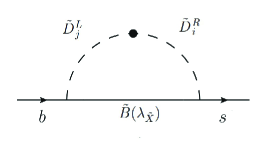
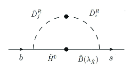
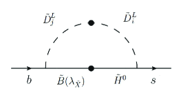
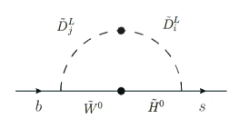
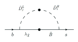
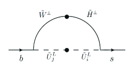
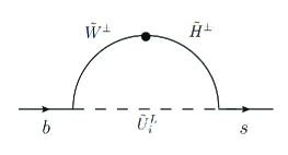
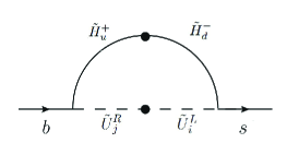
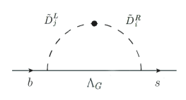
Figure 1: Self-energy Feynman diagrams for $b\rightarrow s\gamma$ in the MIA.

To obtain the branching ratio, we research one-loop diagrams in Fig. 1. To obtain triangle diagrams, the photon should be attached to all inner lines with electric charge. In this case, the coefficients of $\mathcal{O}_{7}$ and $\tilde{\mathcal{O}}_{7}$ can be extracted from the amplitudes of these diagrams of $b\to s\gamma$. Similarly, the coefficients of $\mathcal{O}_{8}$ and $\tilde{\mathcal{O}}_{8}$ can be obtained from the diagrams of $b\rightarrow sg$ with gluons attached to all the inner lines with color charge. We give the following two basic functions:

$$f(x,y,z)=-\frac{\rm i}{16\pi^{2}}\big{[}\frac{x\log x}{(x-y)(x-z)}-\frac{y\log y}{(y-x)(y-z)}-\frac{z\log z}{(z-x)(z-y)}\big{]},$$ (51)

$$g(x,y,z,t)=\frac{1}{z-t}\Big{(}f(x,y,z)-f(x,y,t)\Big{)}.$$ (52)

1. The one-loop contributions from $\tilde{B}(\lambda_{\tilde{X}})$-$\tilde{D}^{L}_{j}$-$\tilde{D}^{R}_{i}$ $(i=2,~{}j=3)$.

$$C_{7}^{1}(\tilde{D}^{L}_{j},\tilde{D}^{R}_{i},\tilde{B})=\frac{1}{216}\frac{{T_{d}}^{ij}v\cos{\beta}}{\mathcal{A}m_{b}\Lambda^{3}}g_{3}^{2}g_{1}^{2}\sqrt{x_{1}}I_{1}(x_{1},x_{\tilde{D}^{L}_{j}},x_{\tilde{D}^{R}_{i}}),$$ (53)

$$C_{7}^{2}(\tilde{D}^{L}_{j},\tilde{D}^{R}_{i},\lambda_{\tilde{X}})=\frac{1}{432}\frac{{T_{d}}^{ij}v\cos{\beta}}{\mathcal{A}m_{b}\Lambda^{3}}g_{3}^{2}(2g_{YX}^{2}+3g_{YX}g_{X})\sqrt{x_{\lambda_{\tilde{X}}}}I_{1}(x_{\lambda_{\tilde{X}}},x_{\tilde{D}^{L}_{j}},x_{\tilde{D}^{R}_{i}}),$$ (54)

$$C_{8}^{1}(\tilde{D}^{L}_{j},\tilde{D}^{R}_{i},\tilde{B})=\frac{1}{216}\frac{{T_{d}}^{ij}v\cos{\beta}}{\mathcal{A}m_{b}\Lambda^{3}}g_{3}^{3}g_{1}^{2}\sqrt{x_{1}}I_{1}(x_{1},x_{\tilde{D}^{L}_{j}},x_{\tilde{D}^{R}_{i}}),$$ (55)

$$C_{8}^{2}(\tilde{D}^{L}_{j},\tilde{D}^{R}_{i},\lambda_{\tilde{X}})=\frac{1}{432}\frac{{T_{d}}^{ij}v\cos{\beta}}{\mathcal{A}m_{b}\Lambda^{3}}g_{3}^{3}(2g_{YX}^{2}+3g_{YX}g_{X})\sqrt{x_{\lambda_{\tilde{X}}}}I_{1}(x_{\lambda_{\tilde{X}}},x_{\tilde{D}^{L}_{j}},x_{\tilde{D}^{R}_{i}}),$$ (56)

in which, $m$ stands for the particle mass, with $x=\frac{m^{2}}{\Lambda^{2}}$. The coefficient $\mathcal{A}$ is equal to $\frac{1}{G_{F}V_{32}^{*}V_{33}}$ and $\Lambda$ represents the energy scale. The function $I_{1}(x,y,z)$ is

$$I_{1}(x,y,z)=-\Big{(}\frac{z}{2}\frac{\partial^{2}}{\partial z^{2}}+\frac{y}{2}\frac{\partial^{2}}{\partial y^{2}}+\frac{\partial}{\partial z}+y\frac{\partial^{2}}{\partial y\partial z}\Big{)}f(x,y,z).$$ (57)

2. The one-loop contributions from $\tilde{B}(\lambda_{\tilde{X}})$-$\tilde{H}^{0}$-$\tilde{D}^{R}_{j}$-$\tilde{D}^{R}_{i}$ $(i=2,~{}j=3)$.

Fig.s 1-1 are all computed with the same method of coefficients and the functions required in the process, so here we take Fig. 1 as an example.

$$C_{7}^{3}(\tilde{D}^{R}_{j},\tilde{D}^{R}_{i},\tilde{B},\tilde{H}^{0})=\frac{\sqrt{2}}{72}\frac{m_{s}\Delta^{RR}_{ij}(\tilde{D})}{\mathcal{A}m_{b}\Lambda^{4}}g_{3}^{2}g_{1}^{2}\tan{\beta}\sqrt{x_{1}x_{\mu^{\prime}_{H}}}I_{2}(x_{1},x_{\tilde{D}^{R}_{j}},x_{\tilde{D}^{R}_{i}},x_{\mu^{\prime}_{H}}),$$ (58)

$$C_{7}^{4}(\tilde{D}^{R}_{j},\tilde{D}^{R}_{i},\lambda_{\tilde{X}},\tilde{H}^{0})=\frac{\sqrt{2}}{288}\frac{m_{s}\Delta^{RR}_{ij}(\tilde{D})}{\mathcal{A}m_{b}\Lambda^{4}}g_{3}^{2}(2g_{YX}+3g_{X})(g_{YX}+g_{X})$$

$$\hskip 122.34692pt\times\tan{\beta}\sqrt{2x_{\lambda_{\tilde{X}}}x_{\mu^{\prime}_{H}}}I_{2}(x_{\lambda_{\tilde{X}}},x_{\tilde{D}^{R}_{j}},x_{\tilde{D}^{R}_{i}},x_{\mu^{\prime}_{H}}),$$ (59)

$$C_{8}^{3}(\tilde{D}^{R}_{j},\tilde{D}^{R}_{i},\tilde{B},\tilde{H}^{0})=\frac{\sqrt{2}}{72}\frac{m_{s}\Delta^{RR}_{ij}(\tilde{D})}{\mathcal{A}m_{b}\Lambda^{4}}g_{3}^{3}g_{1}^{2}\tan{\beta}\sqrt{x_{1}x_{\mu^{\prime}_{H}}}I_{2}(x_{1},x_{\tilde{D}^{R}_{j}},x_{\tilde{D}^{R}_{i}},x_{\mu^{\prime}_{H}}),$$ (60)

$$C_{8}^{4}(\tilde{D}^{R}_{j},\tilde{D}^{R}_{i},\lambda_{\tilde{X}},\tilde{H}^{0})=\frac{\sqrt{2}}{288}\frac{m_{s}\Delta^{RR}_{ij}(\tilde{D})}{\mathcal{A}m_{b}\Lambda^{4}}g_{3}^{3}(2g_{YX}+3g_{X})(g_{YX}+g_{X})$$

$$\hskip 122.34692pt\times\tan{\beta}\sqrt{2x_{\lambda_{\tilde{X}}}x_{\mu^{\prime}_{H}}}I_{2}(x_{\lambda_{\tilde{X}}},x_{\tilde{D}^{R}_{j}},x_{\tilde{D}^{R}_{i}},x_{\mu^{\prime}_{H}}),$$ (61)

in which, $\mu_{H}^{\prime}=\frac{\lambda_{H}v_{S}}{\sqrt{2}}+\mu$ and $x_{\mu^{\prime}_{H}}=\frac{\mu_{H}^{\prime 2}}{\Lambda^{2}}$. The function $I_{2}(x,y,z,t)$ is

$$I_{2}(x,y,z,t)=-\big{[}\frac{z}{2}\frac{\partial^{2}}{\partial z^{2}}+\frac{y}{2}\frac{\partial^{2}}{\partial y^{2}}+\frac{\partial}{\partial z}+y\frac{\partial^{2}}{\partial y\partial z}\big{]}g(x,y,z,t).$$ (62)

3. The one-loop contributions from $\tilde{H}^{\pm}$-$\tilde{W}^{\pm}$-$\tilde{U}^{L}_{j}$-$\tilde{U}^{L}_{i}$.

$$C_{7}^{5}(\tilde{U}^{L}_{j},\tilde{U}^{L}_{i},\tilde{H}^{\pm},\tilde{W}^{\pm})=\frac{\sqrt{2}}{4}\sum_{i,j=1}^{3}\frac{m_{s}\Delta^{LL}_{ij}(\tilde{U})}{\mathcal{A}vm_{b}\Lambda^{3}}V^{*}_{2j}V_{3i}g_{3}^{2}g_{2}\Big{\{}\sqrt{x_{2}}I_{3}(x_{\mu^{\prime}_{H}},x_{\tilde{U}^{L}_{j}},x_{\tilde{U}^{L}_{i}},x_{2})$$

$$\hskip 122.34692pt+x_{2}\sqrt{x_{\mu^{\prime}_{H}}}\tan{\beta}I_{4}(x_{\mu^{\prime}_{H}},x_{\tilde{U}^{R}_{j}},x_{\tilde{U}^{R}_{i}},x_{2})\Big{\}},$$ (63)

$$C_{7}^{6}(\tilde{U}^{L}_{j},\tilde{U}^{L}_{i},\tilde{H}^{\pm},\tilde{W}^{\pm})=\frac{\sqrt{2}}{6}\sum_{i,j=1}^{3}\frac{m_{s}\Delta^{LL}_{ij}(\tilde{U})}{\mathcal{A}vm_{b}\Lambda^{3}}V^{*}_{2j}V_{3i}g_{3}^{2}g_{2}\Big{\{}\sqrt{x_{2}}I_{3}(x_{\mu^{\prime}_{H}},x_{\tilde{U}^{L}_{j}},x_{\tilde{U}^{L}_{i}},x_{2})$$

$$\hskip 122.34692pt+x_{2}\sqrt{x_{\mu^{\prime}_{H}}}\tan{\beta}I_{2}(x_{\mu^{\prime}_{H}},x_{\tilde{U}^{L}_{j}},x_{\tilde{U}^{L}_{i}},x_{2})\Big{\}},$$ (64)

$$C_{8}^{5}(\tilde{U}^{L}_{j},\tilde{U}^{L}_{i},\tilde{H}^{\pm},\tilde{W}^{\pm})=\frac{\sqrt{2}}{6}\sum_{i,j=1}^{3}\frac{m_{s}\Delta^{LL}_{ij}(\tilde{U})}{\mathcal{A}vm_{b}\Lambda^{3}}V^{*}_{2j}V_{3i}g_{3}^{3}g_{2}\Big{\{}\sqrt{x_{2}}I_{3}(x_{\mu^{\prime}_{H}},x_{\tilde{U}^{L}_{j}},x_{\tilde{U}^{L}_{i}},x_{2})$$

$$\hskip 122.34692pt+x_{2}\sqrt{x_{\mu^{\prime}_{H}}}\tan{\beta}I_{2}(x_{\mu^{\prime}_{H}},x_{\tilde{U}^{L}_{j}},x_{\tilde{U}^{L}_{i}},x_{2})\Big{\}}.$$ (65)

The functions $I_{3}(x,y,z,t)$ and $I_{4}(x,y,z,t)$ are

$$I_{3}(x,y,z,t)=-\big{[}1+2y\frac{\partial}{\partial y}+2z\frac{\partial}{\partial z}+\frac{y^{2}}{2}\frac{\partial^{2}}{\partial y^{2}}+\frac{z^{2}}{2}\frac{\partial^{2}}{\partial z^{2}}+yz\frac{\partial z^{2}}{\partial y\partial z}\big{]}g(x,y,z,t),$$ (66)

$$I_{4}(x,y,z,t)=\big{[}\frac{\partial}{\partial y}+2\frac{\partial}{\partial z}+\frac{y}{2}\frac{\partial^{2}}{\partial y^{2}}+\frac{z}{2}\frac{\partial^{2}}{\partial z^{2}}+y\frac{\partial^{2}}{\partial y\partial z}\big{]}g(x,y,z,t).$$ (67)

Similar to the third case, $C_{7}^{7}$, $C_{7}^{8}$, $C_{8}^{6}$ can be extracted from Fig. 1, and calculation process and form are the same as those of $C_{7}^{5}$, $C_{7}^{6}$, $C_{8}^{5}$. We don’t repeat them here.

4. The one-loop contributions from $\tilde{H}^{\pm}$-$\tilde{W}^{\pm}$-$\tilde{U}^{L}_{i}$.

$$C_{7}^{7}(\tilde{U}^{L}_{i},\tilde{H}^{\pm},\tilde{W}^{\pm})=\frac{\sqrt{2}}{4}\sum_{i=1}^{3}\frac{m_{s}}{\mathcal{A}vm_{b}\Lambda}V^{*}_{2i}V_{3i}g_{3}^{2}g_{2}\Big{\{}x_{2}\sqrt{x_{\mu^{\prime}_{H}}}\tan{\beta}I_{5}(x_{\tilde{U}^{L}_{i}},x_{2},x_{\mu^{\prime}_{H}})$$

$$\hskip 102.43008pt+\sqrt{x_{2}}I_{6}(x_{\tilde{U}^{L}_{i}},x_{2},x_{\mu^{\prime}_{H}})\Big{\}},$$ (68)

$$C_{7}^{8}(\tilde{U}^{L}_{i},\tilde{H}^{\pm},\tilde{W}^{\pm})=\frac{\sqrt{2}}{6}\sum_{i=1}^{3}\frac{m_{s}}{\mathcal{A}vm_{b}\Lambda}V^{*}_{2i}V_{3i}g_{3}^{2}g_{2}\Big{\{}x_{2}\sqrt{x_{\mu^{\prime}_{H}}}\tan{\beta}I_{7}(x_{\mu^{\prime}_{H}},x_{2},x_{\tilde{U}^{L}_{i}})$$

$$\hskip 102.43008pt-\sqrt{x_{2}}I_{8}(x_{\mu^{\prime}_{H}},x_{2},x_{\tilde{U}^{L}_{i}})\Big{\}},$$ (69)

$$C_{8}^{6}(\tilde{U}^{L}_{i},\tilde{H}^{\pm},\tilde{W}^{\pm})=\frac{\sqrt{2}}{6}\sum_{i=1}^{3}\frac{m_{s}}{\mathcal{A}vm_{b}\Lambda}V^{*}_{2i}V_{3i}g_{3}^{3}g_{2}\Big{\{}x_{2}\sqrt{x_{\mu^{\prime}_{H}}}\tan{\beta}I_{7}(x_{\mu^{\prime}_{H}},x_{2},x_{\tilde{U}^{L}_{i}})$$

$$\hskip 102.43008pt-\sqrt{x_{2}}I_{8}(x_{\mu^{\prime}_{H}},x_{2},x_{\tilde{U}^{L}_{i}})\Big{\}}.$$ (70)

The functions $I_{5}(x,y,z)$, $I_{6}(x,y,z)$, $I_{7}(x,y,z)$ and $I_{8}(x,y,z)$ are

$$I_{5}(x,y,z)=\big{[}\frac{\partial}{\partial y}+2\frac{\partial}{\partial z}+\frac{y}{2}\frac{\partial^{2}}{\partial y^{2}}+\frac{z}{2}\frac{\partial^{2}}{\partial z^{2}}+y\frac{\partial^{2}}{\partial y\partial z}\big{]}f(x,y,z),$$ (71)

$$I_{6}(x,y,z)=\big{[}1+2y\frac{\partial}{\partial y}+2z\frac{\partial}{\partial z}+\frac{y^{2}}{2}\frac{\partial^{2}}{\partial y^{2}}+\frac{z^{2}}{2}\frac{\partial^{2}}{\partial z^{2}}+yz\frac{\partial z^{2}}{\partial y\partial z}\big{]}f(x,y,z),$$ (72)

$$I_{7}(x,y,z)=\big{[}\frac{\partial}{\partial z}+\frac{z}{2}\frac{\partial^{2}}{\partial z^{2}}\big{]}f(x,y,z),~{}~{}~{}~{}I_{8}(x,y,z)=\big{[}1+z\frac{\partial}{\partial z}\big{]}f(x,y,z).$$ (73)

5. The one-loop contributions from $~{}\Lambda_{G}$-$\tilde{D}^{L}_{j}$-$\tilde{D}^{R}_{i}$ $(i=2,~{}j=3)$.

$$C_{7}^{9}(\tilde{D}^{L}_{j},\tilde{D}^{R}_{i},\Lambda_{G})=-\frac{1}{48}\frac{{T_{d}}^{ij}v\cos{\beta}}{\mathcal{A}m_{b}\Lambda^{3}}g_{3}^{4}\sqrt{x_{\Lambda_{G}}}I_{1}(x_{\Lambda_{G}},x_{\tilde{D}^{L}_{j}},x_{\tilde{D}^{R}_{i}}),$$ (74)

$$C_{8}^{7}(\tilde{D}^{L}_{j},\tilde{D}^{R}_{i},\Lambda_{G})=-\frac{1}{16}\frac{{T_{d}}^{ij}v\cos{\beta}}{\mathcal{A}m_{b}\Lambda^{3}}g_{3}^{5}\sqrt{x_{\Lambda_{G}}}I_{7}(x_{\tilde{D}^{L}_{j}},x_{\tilde{D}^{R}_{i}},x_{\Lambda_{G}}),$$ (75)

$$C_{8}^{8}(\tilde{D}^{L}_{j},\tilde{D}^{R}_{i},\Lambda_{G})=-\frac{1}{48}\frac{{T_{d}}^{ij}v\cos{\beta}}{\mathcal{A}m_{b}\Lambda^{3}}g_{3}^{5}\sqrt{x_{\Lambda_{G}}}I_{1}(x_{\Lambda_{G}},x_{\tilde{D}^{L}_{j}},x_{\tilde{D}^{R}_{i}}).$$ (76)

According to the above procedure, we can get the coefficients of all the diagrams in Fig. 1. We add the coefficients of each diagram separately to obtain the Wilson coefficients, and import them into Eq.(50) to obtain the branching ratio.

III.2 Degenerate Result

Assuming that the masses of all the superparticles are almost degenerate, we are able to more intuitively analyze the factors affecting the flavor transition process $b\rightarrow s\gamma$. In other words, we give the one-loop results in the extreme case, where the masses for superparticles ( $M_{1},~{}M_{2},~{}\mu_{H}^{\prime},~{}M_{\Lambda_{G}},~{}M_{\lambda_{\tilde{X}}},~{}M_{\tilde{D}_{L}},~{}M_{\tilde{D}_{R}},~{}M_{\tilde{U}_{L}},~{}M_{\tilde{U}_{R}},~{}M_{BB^{\prime}}$ ) are equal to $M_{SUSY}$:

$$|M_{1}|=|M_{2}|=|\mu_{H}^{\prime}|=|M_{\Lambda_{G}}|=|M_{\lambda_{\tilde{X}}}|=|M_{BB^{\prime}}|$$

$$=M_{\tilde{D}_{L}}=M_{\tilde{D}_{R}}=M_{\tilde{U}_{L}}=M_{\tilde{U}_{R}}=M_{SUSY}.$$ (77)

The functions $I_{i}(i=1\cdots 11)$, $\Delta^{AB}_{ij}(\tilde{Q})(A,B=R,L)$, ${T_{d}}^{ij}$ and ${T_{u}}^{ij}$ are much simplified as

$$I_{1}(1,1,1)=\frac{{\rm i}}{192\pi^{2}},\hskip 42.67912ptI_{2}(1,1,1)=\frac{{\rm i}}{192\pi^{2}},\hskip 39.83368ptI_{3}(1,1,1,1)=-\frac{{\rm i}}{320\pi^{2}},$$

$$I_{4}(1,1,1,1)=-\frac{{\rm i}}{480\pi^{2}},\hskip 22.76228ptI_{5}(1,1,1,1)=\frac{{\rm i}}{480\pi^{2}},\hskip 28.45274ptI_{6}(1,1,1,1)=\frac{{\rm i}}{320\pi^{2}},$$

$$I_{7}(1,1,1,1)=-\frac{{\rm i}}{480\pi^{2}},\hskip 22.76228ptI_{8}(1,1,1)=-\frac{{\rm i}}{192\pi^{2}},\hskip 31.2982ptI_{9}(1,1,1)=-\frac{{\rm i}}{64\pi^{2}},$$

$$I_{10}(1,1,1)=\frac{{\rm i}}{192\pi^{2}},\hskip 39.83368ptI_{11}(1,1,1)=-\frac{{\rm i}}{48\pi^{2}},$$ (78)

$$\hskip 0.28436pt\Delta^{LL}_{ij}(\tilde{D})=M^{2}_{SUSY}\delta^{LL}_{ij}(\tilde{D}),\hskip 5.69046pt\Delta^{RR}_{ij}(\tilde{D})=M^{2}_{SUSY}\delta^{RR}_{ij}(\tilde{D}),\hskip 5.69046pt\Delta^{LL}_{ij}(\tilde{U})=M^{2}_{SUSY}\delta^{LL}_{ij}(\tilde{U}),$$

$${T_{d}}^{ij}=M_{SUSY}\delta^{ij}_{T_{d}},\hskip 51.21504pt{T_{u}}^{ij}=M_{SUSY}\delta^{ij}_{T_{u}}.$$ (79)

To simplify the study, we suppose that the used matrices are symmetric, for example ${T_{d}}^{ij}={T_{d}}^{ji}$.

Then, we obtain the much simplified one-loop results of $C_{7}$ and $C_{8}$

$$C_{7}=\frac{{\rm i}\mathcal{A}g_{3}^{2}}{2304\pi^{2}M_{SUSY}^{2}}\Big{\{}\frac{\tan{\beta}}{15}\delta^{RR}_{23}(\tilde{D})\Big{(}(3g_{X}^{2}+g_{X}g_{YX}-2g_{YX}^{2})\texttt{sign}[M_{\lambda_{\tilde{X}}}\mu_{H}^{\prime}]-2g_{1}^{2}\texttt{sign}[M_{1}\mu_{H}^{\prime}]\Big{)}$$

$$+\frac{\tan{\beta}}{15}\frac{m_{s}}{m_{b}}\delta^{LL}_{23}(\tilde{D})\Big{(}3g_{2}^{2}\texttt{sign}[M_{2}\mu_{H}^{\prime}]-(g_{X}g_{YX}+g_{YX}^{2})\texttt{sign}[M_{\lambda_{\tilde{X}}}\mu_{H}^{\prime}]-g_{1}^{2}\texttt{sign}[M_{1}\mu_{H}^{\prime}]\Big{)}$$

$$+\frac{v\cos{\beta}\delta^{23}_{T_{d}}}{180m_{b}}\Big{(}10g_{1}^{2}\texttt{sign}[M_{1}]+(15g_{X}g_{YX}+10g_{YX}^{2})\texttt{sign}[M_{\lambda_{\tilde{X}}}]-8g_{1}g_{YX}\texttt{sign}[M_{\lambda_{\tilde{X}}}M_{1}M_{BB^{\prime}}]$$

$$-45g_{3}^{2}\texttt{sign}[M_{\Lambda_{G}}]\Big{)}+\frac{\sqrt{2}M_{SUSY}}{v}\frac{m_{s}}{m_{b}}g_{2}\Big{(}2\tan{\beta}\texttt{sign}[\mu_{H}^{\prime}]-\texttt{sign}[M_{2}]\Big{)}\sum_{l,n=1}^{3}V_{2n}^{*}V_{3l}\delta^{LL}_{ln}(\tilde{U})$$

$$-\frac{22m_{s}\texttt{sign}[\mu_{H}^{\prime}]}{5m_{b}v\cos{\beta}}\sum_{i,j=1}^{3}V^{*}_{2i}V_{3j}m_{u_{j}}\delta^{ji}_{T_{u}}\Big{\}},$$ (80)

$$C_{8}=\frac{{\rm i}\mathcal{A}g_{3}^{3}}{240\pi^{2}M_{SUSY}^{2}}\Big{\{}\frac{\tan{\beta}}{12}\delta^{RR}_{23}(\tilde{D})\Big{(}(3g_{X}^{2}+g_{X}g_{YX}-2g_{YX}^{2})\texttt{sign}[M_{\lambda_{\tilde{X}}}\mu_{H}^{\prime}]-2g_{1}^{2}\texttt{sign}[M_{1}\mu_{H}^{\prime}]\Big{)}$$

$$+\frac{\tan{\beta}}{12}\frac{m_{s}}{m_{b}}\delta^{LL}_{23}(\tilde{D})\Big{(}3g_{2}^{2}\texttt{sign}[M_{2}\mu_{H}^{\prime}]-(g_{X}g_{YX}+g_{YX}^{2})\texttt{sign}[M_{\lambda_{\tilde{X}}}\mu_{H}^{\prime}]-g_{1}^{2}\texttt{sign}[M_{1}\mu_{H}^{\prime}]\Big{)}$$

$$+\frac{v\cos{\beta}\delta^{23}_{T_{d}}}{144m_{b}}\Big{(}10g_{1}^{2}\texttt{sign}[M_{1}]+(15g_{X}g_{YX}+10g_{YX}^{2})\texttt{sign}[M_{\lambda_{\tilde{X}}}]-8g_{1}g_{YX}\texttt{sign}[M_{\lambda_{\tilde{X}}}M_{1}M_{BB^{\prime}}]$$

$$-60g_{3}^{2}\texttt{sign}[M_{\Lambda_{G}}]\Big{)}+\frac{\sqrt{2}M_{SUSY}}{4v}\frac{m_{s}}{m_{b}}g_{2}\Big{(}\texttt{sign}[M_{2}]-4\tan{\beta}\texttt{sign}[\mu_{H}^{\prime}]\Big{)}\sum_{l,n=1}^{3}V^{*}_{2n}V_{3l}\delta^{LL}_{ln}(\tilde{U})$$

$$-\frac{2m_{s}\texttt{sign}[\mu_{H}^{\prime}]}{m_{b}v\cos{\beta}}\sum_{i,j=1}^{3}V^{*}_{2i}V_{3j}m_{u_{j}}\delta^{ji}_{T_{u}}\Big{\}}.$$ (81)

It can be found that $\texttt{sign}[M_{1}],~{}\texttt{sign}[M_{2}],~{}\texttt{sign}[M_{\lambda_{\tilde{X}}}],~{}\texttt{sign}[\mu_{H}^{\prime}],~{}\texttt{sign}[M_{G}]$ and $\texttt{sign}[M_{BB^{\prime}}]$ have a certain impact on the corrections of $C_{7}$ and $C_{8}$. According to $1>g_{X}>g_{YX}>0$, we assume $\texttt{sign}[M_{1}]=\texttt{sign}[M_{\lambda_{\tilde{X}}}]=\texttt{sign}[\mu_{H}^{\prime}]=\texttt{sign}[M_{2}]=\texttt{sign}[M_{G}]=\texttt{sign}[M_{BB^{\prime}}]=1$, and get the larger values of $C_{7}$ and $C_{8}$

$$C_{7}=\frac{{\rm i}\mathcal{A}g_{3}^{2}}{2304\pi^{2}M_{SUSY}^{2}}\Big{\{}\frac{\tan{\beta}}{15}\delta^{RR}_{23}(\tilde{D})(3g_{X}^{2}+g_{X}g_{YX}-2g_{YX}^{2}-2g_{1}^{2})+\frac{\tan{\beta}}{15}\frac{m_{s}}{m_{b}}\delta^{LL}_{23}(\tilde{D})$$

$$\times(3g_{2}^{2}-g_{X}g_{YX}-g_{YX}^{2}-g_{1}^{2})+\frac{v\cos{\beta}\delta^{23}_{T_{d}}}{180m_{b}}\big{(}10g_{1}^{2}+15g_{X}g_{YX}+10g_{YX}^{2}-8g_{1}g_{YX}-45g_{3}^{2}\big{)}$$

$$+\frac{\sqrt{2}m_{s}M_{SUSY}}{m_{b}v}g_{2}(2\tan{\beta}-1)\sum_{l,n=1}^{3}V_{2n}^{*}V_{3l}\delta^{LL}_{ln}(\tilde{U})-\frac{22m_{s}}{5m_{b}v\cos{\beta}}\sum_{i,j=1}^{3}V_{2i}^{*}V_{3j}m_{u_{j}}\delta^{ji}_{T_{u}}\Big{\}},$$ (82)

$$C_{8}=\frac{{\rm i}\mathcal{A}g_{3}^{3}}{240\pi^{2}M_{SUSY}^{2}}\Big{\{}\frac{\tan{\beta}}{12}\delta^{RR}_{23}(\tilde{D})(3g_{X}^{2}+g_{X}g_{YX}-2g_{YX}^{2}-2g_{1}^{2})+\frac{\tan{\beta}}{12}\frac{m_{s}}{m_{b}}\delta^{LL}_{23}(\tilde{D})$$

$$\times(3g_{2}^{2}-g_{X}g_{YX}-g_{YX}^{2}-g_{1}^{2})+\frac{v\cos{\beta}\delta^{23}_{T_{d}}}{144m_{b}}(10g_{1}^{2}+15g_{X}g_{YX}+10g_{YX}^{2}-8g_{1}g_{YX}-60g_{3}^{2})$$

$$+\frac{\sqrt{2}m_{s}M_{SUSY}}{4m_{b}v}g_{2}(1-4\tan{\beta})\sum_{l,n=1}^{3}V_{2n}^{*}V_{3l}\delta^{LL}_{ln}(\tilde{U})-\frac{2m_{s}}{m_{b}v\cos{\beta}}\sum_{i,j=1}^{3}V_{2i}^{*}V_{3j}m_{u_{j}}\delta^{ji}_{T_{u}}\Big{\}}.$$ (83)

To determine the sensitive parameters affecting the branching ratio more clearly and intuitively, similar method is used to derive $\tilde{C}_{7}$ and $\tilde{C}_{8}$ in Eq.(50). Then in combination with the degenerate results in Eq.(82), Eq.(83) and Eq.(79), we set $M_{SUSY}=\mu_{H}^{\prime},~{}g_{YX}=0.1,~{}g_{X}=0.5,~{}\Delta^{RR}_{23}(\tilde{D})=\Delta^{LL}_{23}(\tilde{D})=1\times 10^{4}~{}{\rm{GeV}^{2}},~{}\Delta^{LL}_{ij}(\tilde{U})=4.2\times 10^{4}~{}{\rm{GeV}^{2}}(i\neq j~{}{\rm and}~{}i,j=1,2,3)$ and $\Delta^{LL}_{ii}(\tilde{U})=5\times 10^{6}~{}{\rm GeV^{2}}~{}(i=1,2,3)$ to obtain the following figures:

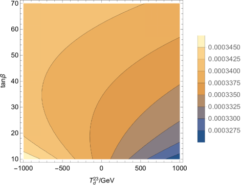
Figure 2: With ${T_{u}}^{23}=-650~{}{\rm GeV}$ and $\mu=1000~{}{\rm GeV}$, the effects of $\tan{\beta}$ and ${T_{d}}^{23}$ on $Br(\bar{B}\rightarrow X_{s}\gamma)$. The x-axis denotes the range of ${T_{d}}^{23}$ is from $-1000~{}{\rm GeV}$ to $1000~{}{\rm GeV}$, and the y-axis represents $10<\tan\beta<70$. The different colors of the rightmost icon correspond to the values of $Br(\bar{B}\rightarrow X_{s}\gamma)$.

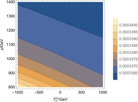
Figure 3: With ${T_{d}}^{23}=600~{}{\rm GeV}$ and $\tan\beta=50$, the effects of $\mu$ and ${T_{u}}^{23}$ on $Br(\bar{B}\rightarrow X_{s}\gamma)$. The x-axis denotes the range of ${T_{u}}^{23}$ is from $-1000~{}{\rm GeV}$ to $1000~{}{\rm GeV}$, and the y-axis represents $800~{}{\rm GeV}<\mu<1400~{}{\rm GeV}$. The different colors of the rightmost icon correspond to the values of $Br(\bar{B}\rightarrow X_{s}\gamma)$.

Combined with Fig. 2 and Fig. 3, it can be seen that $\tan{\beta}$, $\mu$, ${T_{d}}^{23}$ and ${T_{u}}^{23}$ have a significant impact on the results. In Fig. 2, we can see that $Br(\bar{B}\rightarrow X_{s}\gamma)$ increases as the $\tan{\beta}$ increases. The reason can be found in Eq.(82) and Eq.(83). $\tan{\beta}$ is almost always in the numerator, so it is proportional to the result. When $\tan\beta=40$ and ${T_{d}}^{23}=-600~{}{\rm GeV}$, $Br(\bar{B}\rightarrow X_{s}\gamma)$ reaches $3.4\times 10^{-4}$. Compared to the influence of ${T_{d}}^{23}$, $\tan\beta$ obviously has stronger influence. In our hypothesis, $M_{SUSY}$ is equal to $\mu_{H}^{\prime}$, and $\mu$ is proportional to $\mu_{H}^{\prime}$. In Eq.(82) and Eq.(83), $M_{SUSY}$ is inversely proportional to the result. Thus, $\mu$ should be inversely proportional to the result, which can be demonstrated in Fig. 3. When $\mu=800~{}{\rm GeV}$ and ${T_{u}}^{23}=-730~{}{\rm GeV}$, the branching ratio reaches $3.4\times 10^{-4}$. And the influence of $\mu$ is greater than that of ${T_{u}}^{23}$. At the same time, as the values of FCNC sources $\Delta^{LL}_{ij}(\tilde{D}),~{}\Delta^{RR}_{ij}(\tilde{D})$ and $\Delta^{LL}_{ij}(\tilde{U})$ go up, the result also grows. But they have gentle influence on the result, which is not shown here. In summary, we can get the sensitive parameters including $\tan{\beta}$, $\mu$, ${T_{d}}^{23}$ and ${T_{u}}^{23}$.

IV numerical results

To study $Br(\bar{B}\rightarrow X_{s}\gamma)$, we consider the mass constraint for the $Z^{\prime}$ boson ($M_{Z^{\prime}}>5.1$ TeV) Zp5d1 from the latest Large Hadron Collider (LHC) data LHC1 ; LHC2 ; LHC3 ; LHC4 ; LHC5 ; LHC6 ; LHC7 . The constraints $M_{Z^{\prime}}/g_{X}\geq 6~{}{\rm TeV}$ and $\tan\beta_{\eta}<1.5$ are also taken into account. According to the research in Ref. gluino , we take the mass of gluino more than 2 TeV. The parameters are used to make the scalar lepton masses larger than 700 GeV, and chargino masses larger than 1100 GeV, and the scalar quark masses greater than 2000 GeV. Ref. tan1 and Ref. tan2 discuss parameter space for $b\to s\gamma$ under various models, and in their data analysis the value of $\tan\beta$ is relatively high. Considering that $U(1)_{X}$SSM has more parameters and larger adjustment space of parameters, we tend to choose a large value of $\tan\beta$.

In this section, we discuss the numerical results of branching ratio with some assumptions. Other free parameters introduced in the $U(1)_{X}$SSM are set to

$$g_{X}=0.4,~{}g_{YX}=0.1,~{}\lambda_{H}=0.1,~{}v_{S}=3.5~{}{\rm TeV},~{}T_{u11}=T_{u22}=T_{u33}=3~{}{\rm TeV},$$

$$M_{1}=1~{}{\rm TeV},~{}M_{2}=1.1~{}{\rm TeV},~{}M_{\lambda_{\tilde{X}}}=1.4~{}{\rm TeV},~{}M_{G}=2.1~{}{\rm TeV},~{}M_{BB^{\prime}}=0.8~{}{\rm TeV}.$$ (84)

After roughly determining the sensitive parameters, in order to study the influence of parameters on $Br(\bar{B}\rightarrow X_{s}\gamma)$ better, we also need to study before degenerate. To show the numerical results clearly, we draw the relation diagrams and scatter diagrams of $Br(\bar{B}\rightarrow X_{s}\gamma)$ with the parameters of the $U(1)_{X}$SSM.

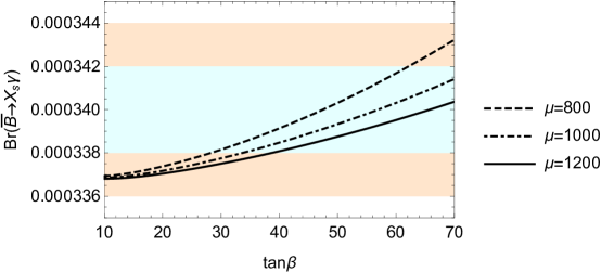
Figure 4: $Br(\bar{B}\rightarrow X_{s}\gamma)$ versus $\tan{\beta}$ with $\Delta^{ij}=3\times 10^{5}~{}{\rm GeV^{2}}$.

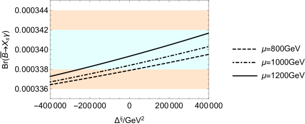
Figure 5: $Br(\bar{B}\rightarrow X_{s}\gamma)$ versus $\Delta^{ij}$ with $\tan\beta=60$.

Fig. 4 shows the relationship between $\tan{\beta}$ and $Br(\bar{B}\rightarrow X_{s}\gamma)$, where $Br(\bar{B}\rightarrow X_{s}\gamma)$ increases with the enlarging $\tan{\beta}$. As the lines in the figure go from bottom to top, the value of $\mu$ decreases gradually. Meanwhile, under the same $\tan{\beta}$, the smaller the $\mu$ is, the larger the value of $Br(\bar{B}\rightarrow X_{s}\gamma)$ is. This is the same as the conclusion of degenerate results. When the value of $\mu$ decreases, the influence of $\tan{\beta}$ gradually becomes more significant. Since the influences of some FCNC sources are small, we set $\Delta^{LL}_{ij}(\tilde{D}),~{}\Delta^{RR}_{ij}(\tilde{D})$ and $\Delta^{LL}_{ij}(\tilde{U})$ to be equal in the drawing of the diagram, and their values are represented by $\Delta^{ij}(i\neq j)$, so as to get Fig. 5. The result is proportional to $\Delta^{ij}$. When $\Delta^{ij}=1.3\times 10^{5}~{}{\rm GeV}^{2}$ and $\mu=800~{}{\rm GeV}$, $Br(\bar{B}\rightarrow X_{s}\gamma)$ reaches $3.4\times 10^{-4}$. Compared with the degenerate result, the influence degree of some parameters on the result has changed. For example, the effects of ${T_{d}}^{23}$ and ${T_{u}}^{23}$ are reduced in precise results. But $\Delta^{ij}$, which have less effect on the degenerate result, have more effect here.

For more multidimensional analysis of sensitive parameters, we draw the scatter points in Figs. 6 - 8. Under the premise of current limit on flavor transition process $b\rightarrow s\gamma$, we select the parameter ranges as follows:

$$\tan{\beta}=10\sim 70,\hskip 68.28644pt{T_{d}}^{23}=-1000\sim 1000~{}{\rm GeV},$$

$$\mu=800\sim 1300~{}{\rm GeV},\hskip 39.83368pt\Delta^{ij}=(-4.0\sim 4.0)\times 10^{5}~{}{\rm{GeV}^{2}}.$$ (85)

In Figs. 6 - 8, $\blacklozenge$ mean the value of $Br(\bar{B}\rightarrow X_{s}\gamma)$ less than $3.37\times 10^{-4}$, $\blacktriangle$ mean $Br(\bar{B}\rightarrow X_{s}\gamma)$ in the range of $3.37\times 10^{-4}$ to $3.39\times 10^{-4}$, $\blacksquare$ show $3.39\times 10^{-4}$ $\leq Br(\bar{B}\rightarrow X_{s}\gamma)$.

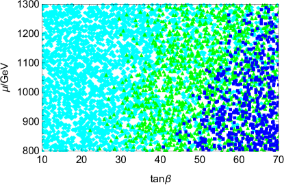
Figure 6: The effects of $\tan\beta$ and $\mu$ on $Br(\bar{B}\rightarrow X_{s}\gamma)$.

Fig. 6 shows the relationship between $\tan\beta$ and $\mu$, and it can be seen that the largest area is occupied by $\blacklozenge$. $\blacksquare$ are mainly concentrated on the right side of the image and decrease with the increase of $\mu$ or the decrease of $\tan\beta$. When $\tan\beta$ is greater than 45, the result is easier to get to $3.40\times 10^{-4}$. Moreover, the three markers $\blacklozenge$, $\blacktriangle$ and $\blacksquare$ have clear distribution boundaries, and $\tan\beta$ has a greater impact on the results.

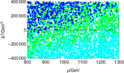
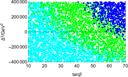
Figure 7: The effects of $\mu$ and $\Delta^{ij}$ on $Br(\bar{B}\rightarrow X_{s}\gamma)$(a); the effects of $\tan\beta$ and $\Delta^{ij}$ on $Br(\bar{B}\rightarrow X_{s}\gamma)(b).$

Fig. 7 shows the relationship between $\mu$ and $\Delta^{ij}$, and Fig. 7 is the relationship between $\tan\beta$ and $\Delta^{ij}$. It can be further seen from the figure that $\tan\beta$ has more obvious influence than $\mu$, because the distribution of midpoints in Fig. 7 is not as clear as that in Fig. 7. For example marker $\blacklozenge$, in Fig. 7, marker $\blacklozenge$ are widely distributed. In contrast, the markers in Fig. 7 are mainly concentrated in the lower left part, and there is no marker $\blacklozenge$ in the upper right part. Combining the two graphs, $\Delta^{ij}$ increase and so does the branching ratio. And when $\Delta^{ij}$ are greater than $-1\times 10^{-5}~{}{\rm GeV^{2}}$, it is easier to reach $3.40\times 10^{-4}$.

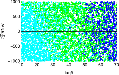
Figure 8: The effect of $\tan\beta$ and $T_{d}^{23}$ on $Br(\bar{B}\rightarrow X_{s}\gamma)$.

The relationship between ${T_{d}}^{23}$ and $\tan\beta$ is shown in Fig. 8. It can be seen that the results increase with the enlarging ${T_{d}}^{23}$. However, when $\tan\beta$ increases to a certain extent, the influence of ${T_{d}}^{23}$ turns weak gradually.

V discussion and conclusion

The $U(1)_{X}$SSM has new superfields including right-handed neutrinos $\hat{\nu}_{i}$ and three Higgs superfields $\hat{\eta},~{}\hat{\bar{\eta}},~{}\hat{S}$, and its local gauge group is $SU(3)_{C}\otimes SU(2)_{L}\otimes U(1)_{Y}\otimes U(1)_{X}$. As an interesting process of FCNC, the flavor transition process $b\rightarrow s\gamma$ is investigated by the MIA within the framework of the $U(1)_{X}$SSM. With effective Hamiltonian method, we present the Wilson coefficients extracted from amplitudes corresponding to the concerned one-loop diagrams. Based on the analytical results, constraints on the parameters are given with the experimental data of $Br(\bar{B}\rightarrow X_{s}\gamma)$. From the data analysis, the flavor transition process $b\rightarrow s\gamma$ has relatively stricter restrictions on the quark flavor violation sources than most other parameters.

We take into account the constraint from the branching ratio. By MIA, we obtain simpler degenerate results. These results contribute to us to more intuitively determine sensitive parameters. It is convenient for subsequent numerical analysis. Through the multi-angle analysis of the values, it is found that the branching ratio is more dependent on the variables $\tan{\beta}$ and $\mu$ in the $U(1)_{X}$SSM. $\Delta^{ij}$ are composed of quark flavor violation sources $\Delta^{LL}_{ij}(\tilde{D}),~{}\Delta^{RR}_{ij}(\tilde{D})$ and $\Delta^{LL}_{ij}(\tilde{U})$, and the influence is also obvious. The effects of ${T_{d}}^{23}$ and ${T_{u}}^{23}$ are relatively insignificant. Parameters that are not graphed, such as $g_{X}$ and $g_{YX}$, have gentle effects on the results. $g_{X},~{}g_{YX},~{}g_{1},~{}g_{2},$ and $g_{3}$ are the coupling constants. $g_{X}$ and $g_{YX}$ only appear in some part of analytical result. So the impact of $g_{X}$ and $g_{YX}$ is relatively small. Therefore, we can get the main sensitive parameters that are $\tan\beta$, $\mu$ and the FCNC sources $\Delta^{ij}$. This work is conductive to further research on the $U(1)_{X}$SSM and FCNC.

Acknowledgments

This work is supported by National Natural Science Foundation of China (NNSFC) (No. 12075074), Natural Science Foundation of Hebei Province (A2020201002, A202201022, A2022201017), Natural Science Foundation of Hebei Education Department (QN2022173), Post-graduate’s Innovation Fund Project of Hebei University (HBU2023SS043), the youth top-notch talent support program of the Hebei Province.

Data Availability Statement: The data are available from the corresponding author on reasonable request.

References

(1)
M. Ciuchini, G. Degrassi, P. Gambino and G. F. Giudice, Nucl. Phys. B 527 (1998) 21.
(2)
P. Ciafaloni, A. Romanino and A. Strumia, Nucl. Phys. B 524 (1998) 361.
(3)
F. Borzumati and C. Greub, Phys. Rev. D 58 (1998) 074004.
(4)
S. Bertolini, F. Borzumati, A. Masiero and G. Ridolfi, Nucl. Phys. B 353 (1991) 591.
(5)
R. Barbieri and G.F. Giudice, Phys. Lett. B 309 (1993) 86.
(6)
F. Borzumati, C. Greub, T. Hurth and D. Wyler, Phys. Rev. D 62 (2000) 075005.
(7)
S. Prelovsek and D. Wyler, Phys. Lett. B 500 (2001) 304.
(8)
M. Causse and J. Orloff, Eur. Phys. J. C 23 (2002) 749.
(9)
H.B. Zhang, G.H. Luo, T.F. Feng, S.M. Zhao, T.J. Gao and K.S. Sun, Mod. Phys. Lett.
A 29 (2014) 1450196 [arXiv:1409.6837].
(10)
M. Tanabashi, et al. (Particle Data Group),
Phys. Rev. D 98 (2018) 030001.
(11)
M. Misiak, et al.,
Phys. Rev. Lett. 114 (2015) 221801.
(12)
M. Czakon, P. Fiedler, et al.,
JHEP 168 (2015) [arXiv:1503.01791].
(13)
M. Misiak, et al.,
Phys. Rev. Lett. 98 (2007) 022002.
(14)
M. Misiak and M. Steinhauser,
Nucl. Phys. B 62 (2007) 764.
(15)
K. Chetyrkin, M. Misiak and M. Munz,
Phys. Lett. B 400 (1997) 206-219.
(16)
C. Greub, T. Hurth and D. Wyler,
Phys. Rev. D 54 (1996) 3350-3364.
(17)
K. Adel and Y.P. Yao,
Phys. Rev. D 49 (1994) 4945-4948.
(18)
A. Ali and C. Greub,
Phys. Lett. B 361 (1995) 146-154.
(19)
J. Rosiek,
Phys. Rev. D 41 (1990) 3464 [arXiv:hep-ph/9511250].