Efficient Image Super-Resolution with Feature Interaction Weighted Hybrid Network

Abstract

Recently, great progress has been made in single-image super-resolution (SISR) based on deep learning technology. However, the existing methods usually require a large computational cost. Meanwhile, the activation function will cause some features of the intermediate layer to be lost. Therefore, it is a challenge to make the model lightweight while reducing the impact of intermediate feature loss on the reconstruction quality. In this paper, we propose a Feature Interaction Weighted Hybrid Network (FIWHN) to alleviate the above problem. Specifically, FIWHN consists of a series of novel Wide-residual Distillation Interaction Blocks (WDIB) as the backbone, where every third WDIBs form a Feature shuffle Weighted Group (FSWG) by mutual information mixing and fusion. In addition, to mitigate the adverse effects of intermediate feature loss on the reconstruction results, we introduced a well-designed Wide Convolutional Residual Weighting (WCRW) and Wide Identical Residual Weighting (WIRW) units in WDIB, and effectively cross-fused features of different finenesses through a Wide-residual Distillation Connection (WRDC) framework and a Self-Calibrating Fusion (SCF) unit. Finally, to complement the global features lacking in the CNN model, we introduced the Transformer into our model and explored a new way of combining the CNN and Transformer. Extensive quantitative and qualitative experiments on low-level and high-level tasks show that our proposed FIWHN can achieve a good balance between performance and efficiency, and is more conducive to downstream tasks to solve problems in low-pixel scenarios.

1 Introduction

Single-image super-resolution (SISR) aims to reconstruct a high-resolution (HR) image from the degraded low-resolution (LR) image. In recent years, SISR is receiving increasing attention as high-resolution images are required for various computer vision tasks, such as medical image analysis, security surveillance, and autonomous driving [1, 2]. However, it is still a challenging task since it is an inverse problem. Recently, the appealing rise of deep neural networks has further advanced the development of SISR. For example, SRCNN [3] was pioneering work that first used neural networks for image super-resolution, using only a three-layer convolutional network but outperforming other sparse representation-based methods by a large margin. VDSR [4] increased the model depth to 20 layers and achieved better performance. Subsequently, a range of approaches [5, 6] relying on stacking network depth to achieve better performance was proposed. However, the computational overhead of these methods is so large that they cannot be applied to realistic scenarios. For example, the EDSR [5] has more than 40M parameters, which results in slow inference speed and difficult deployment. Therefore, lightweight models are urgently needed.

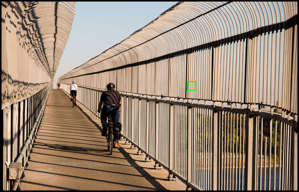
Urban100 ($\times 4$): img024 HR Bicubic Fig. 6 (a) PSNR/SSIM 18.27/0.4629 20.13/0.6647 Fig. 6 (b) Fig. 6 (c) Fig. 6 (d) (Ours) 21.02/0.7024 20.29/0.6628 21.27/0.7134

Figure 1: Visual comparison of different interaction schemes between CNN and Transformer. Existing methods suffer from ambiguous artifacts.

To shrink the model size, most existing approaches focus attention on the design of a rational model structure, including weight sharing [7], multi-scale structures [8, 9], strategies for neural structure search [10], grouped convolution [11, 12]. However, MobileNetV2 [13] has verified that activation functions such as Relu will cause the loss of intermediate information, which is ignored by the existing SISR approaches. Due to the loss of information caused by the activation function, input features will be partially lost during transmission as the depth of the network increases, thus affecting the image reconstruction quality. The motivation to mitigate the loss of information in the middle of the model while lightweight motivates us to propose the Feature Interaction Weighted Hybrid Network (FIWHN). Specifically, we designed wide-residual attention-weighted units, including Wide Identical Residual Weight (WIRW) and Wide Convolutional Residual Weighting (WCRW) as the basic units of our CNN part. It mitigates the impact of feature loss on image reconstruction by obtaining a broader map of features before the activation function to compensate for lost intermediate features. And according to the Nyquist-Shannon sampling theorem, the down-sampling process of LR generation from HR will cause aliasing effects in the frequency domain, which which results in phase distortion. The linear phase property of the lattice structure [14] can eliminate phase distortion and improve the visual effect of the reconstruction [15]. So we chose the Wide-residual Distillation Interaction Blocks (WDIB) with the lattice structure as the block for combining wide-residual attention weighted units. The WDIB has a paired butterfly structure and adaptive combination of wide residual blocks through attention-based connection weights, resulting in a compact network with strong expressive power. Meanwhile, the split-feature distillation plus jump connections brought about by the Wide-residual Distillation Connection (WRDC) framework and the fusion of different classes of features by Self-Calibrating Fusion (SCF) give WDIB better generalisation. Then, Several WDIBs then form a a Feature shuffle Weighted Group (FSWG), which achieves full use of the middle layer information at group level by blending and fusing the features output from each WDIB with each other and then weighting them. It is worth noting that we have introduced a parameter sharing mechanism between every two WDIBs to achieve computational savings.

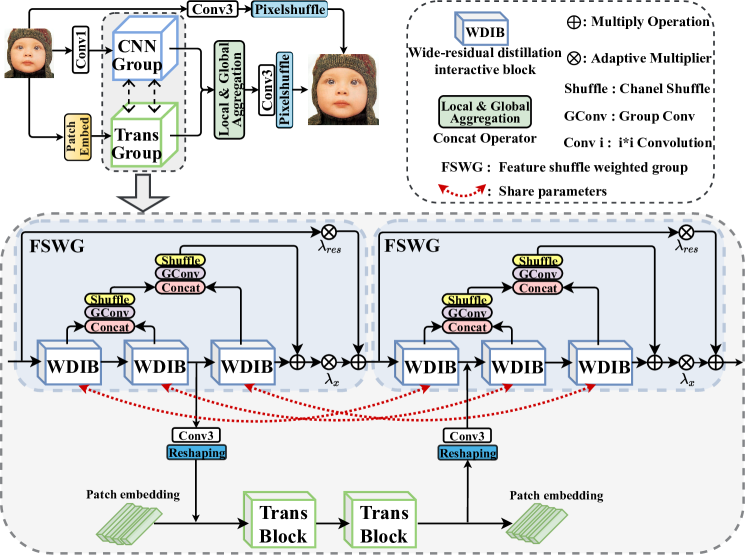
Figure 2: The architecture of the proposed Feature Interaction Weighted Hybrid Network (FIWHN). The ”Trans” in the diagram is short for ”Transformer”.

Recently, we note that Transformer has revealed remarkable performance in many visual tasks [16, 17], and some Transformer-based methods have also shown their great potential for SISR. For instance, SwinIR [18] makes better use of the Transformer’s long-range modeling to accomplish SISR by using a sliding window mechanism to solve the problem of uncorrelated edges between different patches. By using a hybrid network of CNN and Transformer,  [19, 20, 21, 22] show advantages that pure CNN or pure Transformer does not have. Therefore, our method also introduces Transformer to help long-range modeling. It is beneficial for CNN and Transformer to adjust their respective weights by combining the information extracted from each other during the training process, such as  [23]. However, due to the weak ability of existing SISR methods to interact the flow of local information with global information, as shown in Fig. 1, it is easy to generate ambiguous artifacts. Therefore we also explore a better scheme of combining CNN and Transformer, which can further facilitate the interaction between the features extracted by both.

In summary, the main contributions are listed as follows:

• Wide-residual attention weighting units for SISR, including Wide Identical Residual Weighting (WIRW) units and Wide Convolutional Residual Weighting (WCRW) units, are proposed that can mitigate the negative impact of intermediate feature loss through the mechanism of wide residuals.

• In WDIB, we have designed a Wide-residual Distillation Connection (WRDC) framework to enhance information flow by leapfrogging features with different degrees of distillation within the module. Meanwhile, we propose a self-calibrating fusion (SCF) unit to replace the traditional concat operation by an effective feature-weighted interactive fusion.

• An elaborate feature shuffle weighted group (FSWG) is used for pairwise feature shuffle fusion, which consists of a series of interacting WDIBs, and it is also the main fundamental component that forms the CNN part of our model.

• We introduce the Transformer in our proposed approach to facilitate the exchange of global and local middle layer information through a novel interaction framework, and extensive experiments show that our approach can achieve a better balance between efficiency and performance.

In this work, we mainly expand the following contents compared with the conference version [24]:

• To speed up the inference of the model, we increase the dimensionality of the channels, reduce the number of FSWGs modules, and further compress the size of the CNN part by a parameter sharing strategy. Experiments show that such a strategy can exponentially accelerate the inference speed.

• After compressing the volume of the CNN part, we supplement the missing global information of the model with an effective Transformer part. Based on current common combinatorial frameworks, we design a framework that is more conducive to information flow, and extensive experiments show that our proposed combined CNN and Transformer model outperforms existing state-of-the-art methods.

• We have added more detailed experiments and analysis, such as quantitative inference times and more detailed feature visualizations. In addition, the effectiveness of our proposed method is also validated on wider range of super-resolution tasks and downstream tasks. The experiments show that our method is a competitive approach in super-resolution tasks.

2 RELATED WORK

Deep learning methods have made great progress in the task of image super-resolution, and here we focus on the related lightweight SISR model, wide-Residual attention weighting learning, and Transformer-based SISR model.

2.1 Lightweight SISR Model

For SISR to successfully apply to mobile devices, comprehensive concerns have been paid to lightweight models of SISR in research [25, 26, 27, 28]. In summary, the existing methods can be roughly grouped into the following categories: efficient model structure design-based methods [29, 30, 24], pruning or quantification techniques based methods [31], and knowledge distillation based methods [32]. Weight sharing and channel grouping are the methods used to reduce the model size for most of the models related to structural design.  [33, 11] learns the representation of features in different layers by recursive cascading, and then  [34] reuses the features in the intermediate layers by recursive learning. IDN [35] and IMDN [29] use a strategy of channel splitting followed by hierarchical distillation to extract more features at different levels. And FALSR [10] applies neural architecture search (NAS) to the SISR task to get a compact network and achieve good performance by the search strategy, which also provides a new paradigm for us in the structure design-based methods. In addition, model compression methods based on knowledge transfer [32] are gradually being explored in the direction of SISR to improve student model performance by distillation of small student models with pre-trained large teacher models. Finally, for the pruning-based approach,  [36] prunes the secondary model weights to achieve a smaller loss of accuracy while reducing the model size. Our proposed FIWHN belongs to the first class of structural design-based approaches. By discussing the inter-block deployment design relationships between modules, we aim to explore how to combine existing basic units, such as convolutional layers and transformers, to efficiently make the model lightweight. Although work on lightweighting such as this has been extensively explored, there are still many unanswered topical questions that require further research.

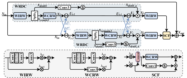
Figure 3: The structure of the proposed Wide-residual Distillation Interaction Block (WDIB). The $M_{i}$ and $M_{i-1}$ in the diagram represent the combination coefficient learning, which can be understood in detail in Fig. 4. And $\odot$ represents the operation of multiplication, ⓢ represents the sigmoid function, $\Theta({x_{i}},{y_{i}})={x_{i}}+{y_{i}}{M_{i}}({y_{i}})$.

2.2 Wide-Residual Weighting Learning

Studies [4, 37] have argued that deeper networks have the potential to be more expressive and to obtain better performance. For example, VDSR [4] uses a 20-layer network, EDSR [5] uses a 65-layer network, and RCAN [37] has a network depth of even more than 800 layers. However, it was then found that the performance of the model does not necessarily get better with the depth of the network but may decrease instead. Studies such as MobileNetV2 [13] point out that the activation functions we use extensively in our models may be responsible for the formation of this feature degradation situation. It points out that the Relu function causes the death of some neurons while increasing the nonlinearity, resulting in the loss of intermediate features, and the model degradation will be more severe as the number of network layers increases. The residual structure represented by ResNet [38] can largely alleviate this feature degradation problem, and this mechanism is also widely used on the task of SISR, but it is still not enough. Since MobileNetV2 [13] also points out that the ReLU activation function causes a large loss of low-dimensional feature information, but less and less information is lost as the dimensionality increases. Meanwhile, WDSR [39] also found that models with wider features before the Relu activation layer can achieve better performance. Motivated by these works, we combine the wide residual mechanism with the attention mechanism, and together with the use of adaptive multipliers that can change the network weights adaptively with training, so our proposed residual block can achieve efficient feature extraction while keeping it lightweight.

2.3 Transformer-based SISR Model

Transformer first appeared in natural language processing(NLP) and has recently demonstrated its powerful capabilities in many tasks [40, 23] in computer vision. The Transformer-based approach for SISR has also been widely studied recently. SwinIR [18] achieved state-of-the-art performance when it first introduced Transformer-based strategies to the SISR task. ESRT [19] and LBNet [20] then combined the lightweight CNN with the lightweight Transformer in the SISR task to achieve a good balance in many metrics. Next, ELAN [21] further improves performance and accelerates the model by grouping multi-scale self-attentive schemes and attention-sharing mechanisms. With the advantage of long-range modeling, Transformer is able to capture global texture features that are difficult to obtain by CNN but beneficial for image recovery. Given Transformer’s impressive performance in SISR tasks and its unique feature extraction capabilities, we introduced it into our approach to complement global features and leverage its efficient feature extraction capabilities to facilitate our model to further recover sharper and more accurate textures.

3 PROPOSED METHOD

In this section, we first give the general structure of the model, including the backbone FSWG of the CNN part and the backbone of the Transformer. And then give our proposed WDIB, which consists of three parts: the wide residual attention weighting unit as the basic unit, the lattice block structure for combining the wide residual attention units, and the WRDC framework and SCF unit. Finally, the combined model of CNN and Transformer and the supervision function for model training are given.

3.1 Feature Interaction Weighting Hybrid Network

FIWHN for SISR. As presented in Fig. 2, it is mainly composed of three parts, shallow feature extraction part, deep feature extraction part, and upsampling part, where the deep feature extraction part is composed of CNN together with the cooperation of Transformer. We use ${I_{LR}}$ and ${I_{SR}}$ to represent the input low-resolution image and super-resolution image, respectively.

Firstly, the shallow feature extraction module consists of a convolutional layer with a boosted convolutional kernel size of 1. The shallow features ${F_{S}}$ can be expressed as:

$${F_{S}}={G_{S}}(X),$$ (1)

where ${G_{S}}(.)$ denotes the shallow feature extraction function. Then, ${F_{S}}$ is sent to the deep feature extraction stage for feature mapping:

$${F_{D}}={G_{Concat}}(C({F_{S}})\leftrightarrow T({F_{S}})),$$ (2)

where $C(.)$ denotes the CNN group, $T(.)$ denotes the Transformer group, $\leftrightarrow$ denotes the information exchange process between CNN and Transformer, and ${G_{Concat}}$ represents the feature fusion process. After extracting and then fusing the local features and global features respectively, we obtain the depth feature ${F_{D}}$.

Feature Shuffe Weighted Group (FSWG). Most of the existing methods connect only the residuals between blocks, and the hierarchy of feature interaction between blocks is often ignored. Therefore, we introduce a feature shuffling and fusion mechanism in FSWG to fuse, group, and shuffle the features of different receiver domains successively. As shown in Fig. 2, the FSWG, as the backbone component of the CNN part, consists of 3 interacting WDIBs. Specifically, we blend and shuffle the adjacent WDIB output features forward progressively. The cascade operation ${G_{CGS}}$ can be represented as:

$${G_{CGS}}={G_{Shuffle}}({G_{GConv}}({G_{Concat}}[{x_{i}},{x_{i+1}}])),$$ (3)

where ${G_{GConv}}$ represents the operation of group convolution, ${G_{Shuffle}}$ represents the operation of channel shuffling, ${x_{i}}$ and ${x_{i+1}}$ represent the output features of the two blocks to be fused respectively. Next, we set up a reasonable group to control the optimal number of graded shuffle fusions. Finally, adaptive multipliers are applied to the fused features between blocks as well as to the original features of the input, respectively, allowing the network to better adjust the weights with training. Defining the input as ${W_{in}}$ and the output as ${W_{out}}$, the process can be represented as:

$${W_{CGS}}={F^{2}}_{CGS}({F^{1}}_{CGS}({W_{1}},{W_{2}}),{W_{3}}),$$ (4)

$${W_{out}}={\lambda_{x}}({W_{CGS}}+{W_{3}})+{\lambda_{res}}{W_{i}n},$$ (5)

where ${W_{i}}$ represents the output of the i-th WDIBs, FCGS represents the function of the i-th ${F^{i}}_{CGS}$, and ${W_{CGS}}$ represents the output features obtained from different blocks after a series of fusion grouping and shuffling.

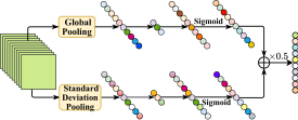
Figure 4: The detail of the combination coefficient learning.

Efficient Transformer (ET). Due to the limited network depth of lightweight models and the fact that convolutional neural networks (CNN) follow a local feature extraction pattern. Under these conditions, the lightweight pure CNN network is far from adequate for reconstructing high-quality images. To improve this problem, we compressed the size of the CNN and introduced an efficient Transformer to learn the long-distance dependence of the images. In terms of details, as show in Fig. 5, we follow ESRT’s [19] design philosophy in terms of multi-headed attention (MHA) so that it takes up less GPU training memory. By splitting the token of Q, K, V ($Q,K,V)\in(B,heads,H*W,C/heads)$ generated by the linear layer along the dimensions of width and height, it can be formulated as the following:

$$\begin{array}[]{l}({Q_{1}}...{Q_{n}}),{\rm{}}({K_{1}}...{K_{n}}),{\rm{}}({V_{1}}...{V_{n}}){\rm{}}={\rm{}}Split(Q,{\rm{}}K,{\rm{}}V).\end{array}$$ (6)

Then, the sub-token obtained after subsequent splitting is matrix multiplied on a field of only $\frac{1}{n}$ (n represents the number of feature splits, and we chose four splits.) of the original perception, effectively reducing the memory consumption. Finally, the sub-attention obtained from the matrix dot product is merged to obtain the final self-attention, and the process can be described as follows:

$$\begin{array}[]{l}{O_{i}}=Attentio{n_{i}}({Q_{i}},{K_{i}},{V_{i}})={\rm{softmax}}(\frac{{{Q_{i}}K_{i}^{T}}}{{\sqrt{{d_{k}}}}}){{\rm{V}}_{i}},\\ \end{array}$$ (7)

$$\begin{array}[]{l}Attention(Q,K,V){\rm{}}={\rm{}}Concat({O_{1}},...,{O_{n}}).\\ \end{array}$$ (8)

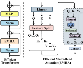
Figure 5: The architecture of the Efficient Transformer (ET).

3.2 Wide-Residual Distillation Interaction Block

Lattice structure. Inspired by the advantages of lattice blocks [30], as shown in Fig. 3, we use this structure to combine wide-residual weighted blocks, which consist of paired butterfly structures that are designed to connect upper and lower features by combining learning coefficients. And each butterfly structure can bring a different combination pattern for the residual units. And we perform jump feature splitting and information refinement while combining residual blocks, and use the idea of information distillation [35, 29] to efficiently perform feature selection and fusion. Specifically, For the input feature ${X_{in}}$, which is fed into the upper and lower branches, we define ${F_{ir}}$ as the WIRW unit and ${F_{cr}}$ as the WCRW unit, and the operation of the upper branch can be described as:

$$\begin{array}[]{l}{X_{remain1}},{X_{distill1}}=Split({F_{ir}}({X_{in}})),\\ \end{array}$$ (9)

$$\begin{array}[]{l}{X_{1}}={F_{cr}}({X_{remain1}}).\\ \end{array}$$ (10)

The upper and lower branches are then connected via the first butterfly mechanism, and the process can be formulated as:

$$\begin{array}[]{l}{V_{i-1}}=\Theta({X_{in}},{X_{1}})={X_{in}}+{X_{1}}M_{{}_{i-1}}^{u}({X_{1}}),\\ \end{array}$$ (11)

$$\begin{array}[]{l}{U_{i-1}}=\Theta({X_{1}},{X_{in}})={X_{1}}+{X_{in}}M_{{}_{i-1}}^{d}({X_{in}}),\\ \end{array}$$ (12)

where $M_{{}_{i-1}}^{u}$ and $M_{{}_{i-1}}^{d}$ represent the two combined coefficient learning mechanisms connecting the upper and lower branches in the first butterfly structure, respectively, and their details can be found in Fig. 4. Compared to the average pooling used in traditional channel attention, the standard difference pooling branch is added here to obtain better visualization, as has been verified in  [29]. Where ${U_{i-1}}$ and ${V_{i-1}}$ represent the output features of the upper and lower branches after passing through the first butterfly structure, respectively. Subsequently, ${U_{i}}$ and ${V_{i}}$ are fed into the second butterfly structure, which proceeds similarly to the first butterfly structure and the process can be expressed as:

$$\begin{array}[]{l}{X_{remain2}},{X_{distill2}}=Split({F_{ir}}({V_{i-1}})),\\ \end{array}$$ (13)

$$\begin{array}[]{l}{X_{2}}={F_{cr}}({X_{remain2}}),\\ \end{array}$$ (14)

$$\begin{array}[]{l}{V_{i}}=\Theta({X_{2}},{U_{i-1}})={X_{2}}+{U_{i-1}}M_{i}^{u}({U_{i-1}}),\\ \end{array}$$ (15)

$$\begin{array}[]{l}{U_{i}}=\Theta({U_{i-1}},{X_{2}})={U_{i-1}}+{X_{2}}M_{{}_{i}}^{d}({X_{2}}).\\ \end{array}$$ (16)

Similar to the previous, ${U_{i}}$ and ${V_{i}}$ represent the output features of the upper and lower branches after the second butterfly structure, respectively, and $M_{i}^{u}$ and $M_{i}^{u}$ represent the combined coefficient learning mechanism above and below the connection of the second butterfly structure. At the same time, the features split out of the upper and lower branches also complete the non-linearization of the coarse features by the operation of convolution plus sigmoid, and the coarse features ${X_{distill\_u}}$ of the upper branch and the coarse features ${X_{distill\_d}}$ of the lower branch are obtained, respectively, and the process can be expressed as:

$$\begin{array}[]{l}{X_{distill\_u}}={F_{sigmoid}}({F_{conv3}}({X_{distill1}})),\\ \end{array}$$ (17)

$$\begin{array}[]{l}{X_{distill\_d}}={F_{sigmoid}}({F_{conv3}}({X_{distill2}})).\\ \end{array}$$ (18)

Next, the obtained coarse features ${X_{distill\_u}}$ and ${X_{distill\_d}}$ interact with the fine features ${U_{i}}$ and ${V_{i}}$ modulated by the attention-based combined coefficient learning mechanism to achieve feature blending with different degrees of refinement. Finally, the blended features ${X_{i}}$ and ${X_{j}}$ are fused using our well-designed Self-Calibration Fusion (SCF) module to jump-start the adaptive fusion of the blended features obtained from the two branches. And the original input features are retained using residual concatenation. It can be formulated as:

$$\begin{array}[]{l}{X_{out}}={F_{SCF}}({F_{ir}}({X_{i}}),{F_{ir}}({X_{j}}))+{X_{in}},\\ \end{array}$$ (19)

where ${F_{SCF}}$ represents the SCF module. As for the fusion method within SCF, the output of the upper and lower branches is first multiplied by the adaptive weights, and then a concat operation is executed. Subsequently, different degrees of refinement is implemented on the fused features, and the various types of information finally obtained make up the reference fused features. Due to the adaptive multipliers in the module that continuously adjust and calibrate the output network weights during training, a better performance than the traditional fusion operation can be achieved.

Wide-Residual Distillation Connection (WRDC). As shown in Fig. 3, the Wide Residual Distillation Connection (WRDC) is the main component of the model, which includes Wide Convolutional Residual Weighting (WCRW), Wide Identical Residual Weighting (WIRW) units, and jump connections for feature refinement. Both WIRW and WCRW introduce a wide range of activation mechanisms to reduce the loss of intermediate layer features and extract richer features with less computation by the idea of wide residuals. For WIRW, specifically, the wide residual mechanism splits the first $3\times 3$ convolution in the original residual into two $1\times 1$ convolutions, and the channel dimension is increased significantly on the first $1\times 1$ convolution to cope with the subsequent activation function and reduce the feature loss. The second $1\times 1$ convolution is then used for channel dimensionality reduction to avoid the huge number of parameters from the $3\times 3$ convolutional layers used to extract features. For the input feature x, the broad features obtained by this process can be expressed as:

$$\begin{array}[]{l}{x_{wide}}={F_{conv3}}({F_{conv1\downarrow}}({F_{relu}}({F_{conv1\uparrow}}(x)))),\\ \end{array}$$ (20)

where ${F_{conv1\uparrow}}$ represents the channel up-dimensioning operation of the first $1\times 1$ convolution, ${F_{conv1\downarrow}}$ represents the channel down-dimensioning operation of the second $1\times 1$ convolution, ${F_{relu}}$ represents the Relu activation function used for nonlinearization, and ${F_{conv3}}$ represents the $3\times 3$ convolution used for feature extraction. Since all the high-dimensional channel operations are performed on the $1\times 1$ convolution, such operations do not cause a large computational load. Subsequently, adaptive multipliers are added to the main branch and the residual branch of the residual block to achieve autonomous adjustment of the weights of the residual block during training. It is worth noting that WCRW has $3\times 3$ convolution layers added to its shortcut path compared to WIRW, allowing it to match the original input channel size after channel splitting. Thus the outputs ${y_{wirw}}$ and ${y_{wcrw}}$ of WIRW and WCRW can be expressed respectively as:

$$\begin{array}[]{l}{y_{wirw}}={\lambda_{x1}}{x_{wide}}+{\lambda_{res1}}x,\\ \end{array}$$ (21)

$$\begin{array}[]{l}{y_{wcrw}}={\lambda_{x2}}{x_{wide}}+{\lambda_{res2}}{F_{conv3}}(x),\\ \end{array}$$ (22)

where ${\lambda_{xk}}$ and ${\lambda_{res2}}$ ($k$=1,2) denote the adaptive weighted multipliers of the k-th wide residual weighted unit. In addition, a convolutional layer is introduced in the distillation connection part to extend the dimensionality of the split channels, and the Sigmoid function nonlinearities of the obtained coarse features to obtain the low-frequency feature maps. Finally, these features are multiplied with the high-frequency feature maps obtained by the dual action of wide residual units plus combined coefficient learning to achieve the interaction of various types of pattern features.

3.3 The Interaction of CNN and Transformer

In SISR tasks, methods based on the interaction of CNN and Transformer have been widely applied recently, and the architecture they are integrated can be roughly divided into the three categories (a), (b), (c) in Fig. 6. Some methods use the structure of (a) and (b) in Fig. 6 by concatenating CNN and Transformer to focus on local and global features in batches, such as ESRT [19], LBNet [20], and CFIN [22], etc. Another class of methods, such as TANet [41], uses the structure of (c) in Fig. 6 to accomplish the feature extraction task in image reconstruction by connecting the CNN and Transformer in parallel and then fusing the extracted local features with the global features. However, most of these methods ignore the issue that the local features extracted from the middle layer of the model are more beneficial to image reconstruction after interacting with the global features. Our proposed interaction approach allows local and global patterns to flow freely in the network, making the two patterns guide each other. Thanks to this interacted approach, our model has the potential for multiple interaction between local and global features, as shown in Fig 6. Compared with the single combined mode of previous methods, our interaction approach is more conducive to improve the generalization of the model and enhance the image reconstruction quality.

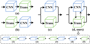
Figure 6: Exploring how to combine CNN and Transformer efficiently and the potential of our method for multiple combinations of both.

3.4 Loss Function

For the pairs $\left\{{I_{LR}^{i},I_{HR}^{i}}\right\}_{i=1}^{N}$ in the training set, the reconstruction loss of our method FIWHN during training can be expressed as:

$$Loss(\theta)=\mathop{{\rm{argmin}}}\limits_{\theta}\frac{1}{N}\sum\limits_{i=1}^{N}{{{\left\|{FIWHN(I_{LR}^{i})-I_{HR}^{i}}\right\|}_{1}}},$$ (23)

where $N$ represents the number of LR-HR pairs in the training set, and $\theta$ represents the parameters size of FIWHN.

4 EXPERIMENTS

In this section, we describe in detail the ablation experiments for each module and the performance of our method for various types of super-resolution tasks.

4.1 Datasets

We use DIV2K [42] as the training set in this experiment, which is a high-definition dataset including images of various natural scenes. It includes 900 high-resolution images, of which the first 800 are used for training and the last 100 for validation. And the LR samples are generated using a double triple downsampling method as used in articles such as  [37]. In addition, we test our method on commonly used benchmark datasets including Set5 [43], Set14 [44], BSDS100 [45], Urban100 [46], and Manga109 [47].

4.2 Implementation Details

For training, we set the initial learning rate to 5e-4 and use the cosine annealing strategy to finally decay to 6.25e-6 at 1000 epochs. The optimizer is the Adam optimizer, where the ${\beta_{1}}$ parameter is set to 0.9 and the ${\beta_{2}}$ parameter is set to 0.999. We randomly crop patches of size 48$\times$48 from the training set as the input for training, while performing data enhancement strategies such as random rotation and random flipping on them. All our training is done using the Pytorch framework on an NVIDIA RTX 2080Ti. In the final model, we set the initial channel to 32 for the CNN part and 144 for the Transformer part, and we use weight normalization [48] after the convolutional layers in the wide residual block to speed up the convergence of the training. It takes about one to two days to train our full model.

For evaluations, we mainly use the commonly used evaluation metrics, including peak signal-to-noise ratio (PSNR) and structural similarity (SSIM). It is worth noting that both metrics are measured on the Y channel on YCbCr space [37]. In addition, for the task of face super-resolution, we introduce two extra key metrics, Learned Perceptual Image Patch Similarity (LPIPS) and Visual Information Fidelity (VIF), to measure the perceptual quality of the face images.

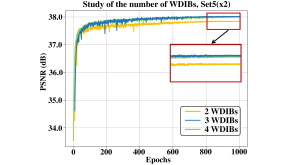
Figure 7: Study of different numbers of WDIBs.

4.3 Ablation Study

The effectiveness of WIRW and WCRW. To compare the superiority of the residual blocks under the broad activation mechanism over the normal residual blocks, we use the basic residual blocks instead of WIRW and WCRW and repositioned them in WDIB, and treat them as the baseline model. The baseline residual block includes two 3$\times$3 convolutions and one relu activation function. To explore the effect of the number of channels before the activation function on the quantitative performance of SR, we set the number of channels before the activation function to 64 and 120, respectively. We can see from TABLE I that: i) FIWHN can achieve better performance and faster inference speed with less number of parameters and Multi-adds compared to the baseline model; ii) by increasing the number of channels before the activation function (case2 and case3), the performance of the model can be further improved with a little additional computational load.

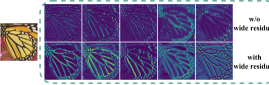
Figure 8: Visualization on the effect of wide residual mechanism on extracted features.

In addition, we also provide visual results to observe the beneficial effects of the wide residual mechanism on feature extraction. As shown in Fig. 8, we depict the feature maps for the normal residual block and our wide residual block, respectively. It can be seen that the features extracted by the normal residual block lost many details in contour texture regions, which are crucial for faithful image recovery. On the contrary, our wide residual mechanism can significantly alleviate the loss of these intermediate useful features mentioned above. This further validates that our proposed WIRW and WCRW can help to recover higher-quality images with more realistic details.

TABLE I: Analysis of the effect of the wide residual mechanism on WIRW and WCRW.

Methods	Channels	Params	Multi-adds	Set5($\times 4$)
				PSNR / Time
Baseline	32	223K	12.69G	31.75 / 7.22ms
FIWHN	64	147K	4.46G	31.76 / 5.72ms
FIWHN	120	175K	9.89G	31.83 / 6.49ms

TABLE II: Impact analysis of different module combinations in the WDIB framework.

Methods	WRDC	SCF	BI	$\otimes$	Params	Multi-adds	Set5($\times 4$)
							PSNR / SSIM
Baseline	✕	✕	✕	✕	59.3K	3.36G	31.17 / 0.8791
Case 1	✓				49.2K	2.11G	31.17 / 0.8799
Case 2		✓			69.5K	3.62G	31.35 / 0.8824
Case 3			✓		59.3K	3.36G	31.22 / 0.8791
Case 4				✓	59.3K	3.36G	31.21 / 0.8794
FIWHN	✓	✓	✓	✓	69.9K	2.57G	31.42 / 0.8835

The effectiveness of WDIB. First, we analyze the internal composition of WDIB in TABLE II, including our proposed modules WRDC (Case 1), SCF (Case 2) and $\otimes$ (adaptive multiplier, Case 4), demonstrating their indispensability in the model composition. From the comparison of case 1, case 2 and baseline, We can see that our proposed WRDC module is able to save about 13$\%$ of the number of parameters and 37$\%$ of the Multi-adds due to the wide residual mechanism, while performing slightly better performance than that of baseline. The SCF module even improves the PSNR value by 0.18 dB with less than 10K parametric gain. Although the adaptive multiplier only improves the PSNR by 0.04 dB compared to baseline, it is worth noting that its usage does not impose any additional computational load and does not slow down the inference process. Ultimately our model improves the performance substantially after aggregating these submodules.

Next, we present in TABLE III a cross-sectional comparison of our proposed WDIB with the sub-block of some methods in terms of PSNR values, model complexity, and inference speed. These methods include state-of-the-art models such as RCAN [37], IMDN [29], RFDN [49], LatticeNet [30], ESRT [19], and LBNet [20]. Since the number of parameters of individual blocks in different methods varies greatly, to make a fair comparison, we stack these blocks to a similar number of parameters and then compare them in all aspects. As can be seen from the table, our proposed WDIB achieves the best performance with less computation. Moreover, due to the parallel structure adopted in the module, our model depth is shallower and the inference speed is the second fastest among these methods. After weighing the model capacity, inference speed, and reconstruction accuracy, WDIB is a better choice to cope with efficient image reconstruction.

The combination structure of FIWHN. The combination structure of our proposed model consists of two main parts. The first is the feature grouping shuffle fusion part of the combined WDIB, which is mainly designed to alleviate the problem that the output are not well communicated between blocks. In TABLE II, we compare the performance of the model with and without Block Interaction (BI) between blocks. Case 3 has only one more BI part compared to the baseline and with almost no increase in computational load. The PSNR value of the small model increases by 0.05 dB. This also illustrates that the communication between blocks benefits image reconstruction. In addition, since the outputs between blocks may suffer from information loss during information transfer, we also explore the optimal number of inter-block feature mixing and fusion. As can be seen from Fig. 7, the performance of the model reaches its best when the number of WDIBs composing FSWG is 3. Therefore, we use three WDIBs to form the FSWG in this work.

TABLE III: Evaluate the effectiveness of our WDIB.

Methods	Depth	Params	Multi-adds	Set5($\times 4$)
				PSNR / Time
RCAB [37]	35	66.8K	3.78G	31.27 / 2.43ms
IMDB [29]	32	60.0K	3.42G	31.40 / 4.37ms
RFDB [49]	24	63.2K	3.51G	31.36 / 3.51ms
LB [30]	39	65.2K	3.66G	31.34 / 4.41ms
HPB [19]	48	64.5K	3.78G	31.36 / 6.81ms
LFFM [20]	25	61.2K	3.47G	31.37 / 3.05ms
WDIB	26	61.0K	2.49G	31.44 / 3.02ms

TABLE IV: Experiments about the performance of various combined CNN and Transformer architectures setting.

Scale	Architecture	Set14	B100	Urban100	Manga109
$\times 4$	Fig. 6 (a)	28.72	27.63	26.40	30.89
	Fig. 6 (b)	28.71	27.64	26.33	30.75
	Fig. 6 (c)	28.61	27.58	26.18	30.56
	ours: (d)	28.76	27.68	26.57	30.93

The second part of the combined structure is combining the CNN with the Transformer. In TABLE IV, we evaluate several combinations as shown in Fig. 6. Compared with simple CNN followed by Transformer or simple Transformer followed by CNN, or simple parallel CNN with Transformer, our scheme achieves better performance. It is worth noting that the combination approach does not affect the overall computational load, and the parallel structure will have a lower model depth and faster inference speed compared to the serial one. These experiments on combination architectures all show that a good combination architecture can significantly enhance model representation ability while imposing little computational load. And also demonstrates that the features in the middle layer, both local-based and global-based, need to be well connected and combined to maximize the model generalization ability. To visualize the effects of CNN and Transformer on the attention area, we provide the feature heat maps at the branch of the model with different structures. As shown in Fig. 9, when the model contains only the CNN part, the attention to the image can only focus on the local area. When the model contains only the Transformer part, it can effectively focus on the global image information but may ignore some local detail information. After integrating CNN and Transformer, it can take into account the local and global areas simultaneously and more details are activated.

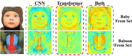
Figure 9: Heat maps about the internal composition of FIWHN.

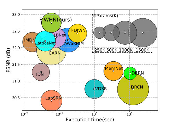
Figure 10: Model inference time studies on Urban100 ($\times 2$).

Model complexity analysis. As shown in Fig. 10, we have made comprehensive comparisons with some state-of-the-art methods in terms of inference time, PSNR performance, and the number of parameters. It can be seen that our method achieves the best performance with a smaller number of parameters. Moreover, it is worth mentioning that our method is one of only halves of the methods that have an average single-image inference speed of fewer than 0.1 seconds. Therefore, we can conclude that our approach achieves a better balance between model complexity, performance, and inference speed compared to other methods.

TABLE V: Analyze the accuracy of face detection and recognition on the CelebA and Helen datasets.

Methods	$CelebA$		$Helen$
	Detection Accuracy${\uparrow}$	Recognition Accuracy${\uparrow}$	Detection Accuracy${\uparrow}$	Recognition Accuracy${\uparrow}$
HR	100$\%$	99.8$\%$	100$\%$	100$\%$
Bicubic	96.5$\%$	19.8$\%$	94.0$\%$	76.0$\%$
SAN [50]	99.7$\%$	95.7$\%$	100$\%$	88.0$\%$
RCAN [37]	99.6$\%$	96.9$\%$	100$\%$	84.0$\%$
HAN [51]	99.7$\%$	96.8$\%$	98.0$\%$	66.0$\%$
SPARNet [52]	99.6$\%$	97.3$\%$	100$\%$	94.0$\%$
IMDN [29]	99.7$\%$	97.5$\%$	96.0$\%$	94.0$\%$
FDIWN [24]	99.7$\%$	97.8$\%$	100$\%$	96.0$\%$
[3pt/3pt] FIWHN(ours)	99.8$\%$	98.6$\%$	100$\%$	98.0$\%$

TABLE VI: Comparison with some Transformer-base methods for $\times 4$ SR. * means this model is pre-trained based on the $\times 2$ setup and the training patch size is set to 64 $\times$ 64 (ours is 48 $\times$ 48 and without pre-training).

Methods	Params	Multi-adds	GPU	Time	Set14	BSD100	Urban100	Manga109	Average
					PSNR / SSIM	PSNR / SSIM	PSNR / SSIM	PSNR / SSIM	PSNR / SSIM
SwinIR* [18]	897K	49.6G	10500M	55ms	28.77 / 0.7858	27.69 / 0.7406	26.47 / 0.7980	30.92 / 0.9151	28.46 / 0.8192
ESRT [19]	751K	67.7G	4191M	34ms	28.69 / 0.7833	27.69 / 0.7379	26.39 / 0.7962	30.75 / 0.9100	28.38 / 0.8160
LBNet [20]	742K	38.9G	6417M	49ms	28.68 / 0.7832	27.62 / 0.7382	26.27 / 0.7906	30.76 / 0.9111	28.30 / 0.8147
CFIN [22]	699K	31.2G	11419M	45ms	28.74 / 0.7849	27.68 / 0.7396	26.39 / 0.7946	30.73 / 0.9124	28.35 / 0.8169
[3pt/3pt] FIWHN(ours)	725K	35.6G	7579M	38ms	28.76 / 0.7849	27.68 / 0.7400	26.57 / 0.7989	30.93 / 0.9131	28.49 / 0.8186

TABLE VII: Average PSNR/SSIM comparison with other advance CNN-based SISR models. The best and the second best results are highlighted and underlined, respectively. ’+’ indicates that the model uses a self-ensemble strategy.

Methods Scale Params Multi-adds Set5 Set14 BSDS100 Urban100 Manga109 PSNR/SSIM PSNR/SSIM PSNR/SSIM PSNR/SSIM PSNR/SSIM IDN [35] $\times 2$ 553K 124.6G 37.83/0.9600 33.30/0.9148 32.08/0.8985 31.27/0.9196 38.01/0.9749 CARN [11] 1592K 222.8G 37.76/0.9590 33.52/0.9166 32.09/0.8978 31.92/0.9256 38.36/0.9765 IMDN [29] 694K 158.8G 38.00/0.9605 33.63/0.9177 32.19/0.8996 32.17/0.9283 38.88/0.9774 AWSRN-M [53] 1063K 244.1G 38.04/0.9605 33.66/0.9181 32.21/ 0.9000 32.23/0.9294 38.66/0.9772 MADNet [54] 878K 187.1G 37.85/0.9600 33.38/0.9161 32.04/0.8979 31.62/0.9233 - MAFFSRN-L [55] 790K 154.4G 38.07/0.9607 33.59/0.9177 32.23/0.9005 32.38/0.9308 - LAPAR-A [56] 548K 171.0G 38.01/0.9605 33.62/0.9183 32.19/0.8999 32.10/0.9283 38.67/0.9772 RFDN [49] 534K 123.0G 38.05/0.9606 33.68/0.9184 32.16/0.8994 32.12/0.9278 38.88/0.9773 GLADSR [57] 812K 187.2G 37.99/0.9608 33.63/0.9179 32.16/0.8996 32.16/0.9283 - LatticeNet+ [30] 756K 165.5G 38.15/0.9610 33.78/0.9193 32.25/0.9004 32.29/0.9291 - SMSR [58] 985K 351.5G 38.00/0.9601 33.64/0.9179 32.17/0.8990 32.19/0.9284 38.76/0.9771 DRSAN [59] 690K 159.3G 38.11/0.9609 33.64/0.9185 32.21/0.9005 32.35/0.9304 - FDIWN [24] 629K 112.0G 38.07/0.9608 33.75/0.9201 32.23/0.9003 32.40/0.9305 38.85/0.9774 LatticeNet-CL [15] 756K 169.5G 38.09/0.9608 33.70/0.9188 32.21/0.9000 32.29/0.9291 - FMEN [60] 748K 172.0G 38.10/0.9609 33.75/0.9192 32.26/0.9003 32.41/0.9311 38.95/0.9778 [3pt/3pt] FIWHN (Ours) 705K 137.7G 38.16/ 0.9613 33.73/0.9194 32.27/ 0.9007 32.75/ 0.9337 39.07/0.9782 FIWHN+ (Ours) 705K 137.7G 38.23/ 0.9615 33.86/ 0.9201 32.33/ 0.9016 32.89/ 0.9350 39.23/ 0.9785 IDN [35] $\times 3$ 553K 56.3G 34.11/0.9253 29.99/0.8354 28.95/0.8013 27.42/0.8359 32.71/0.9381 CARN [11] 1592K 118.8G 34.29/0.9255 30.29/0.8407 29.06/0.8034 28.06/0.8493 33.43/0.9427 IMDN [29] 703K 71.5G 34.36/0.9270 30.32/0.8417 29.09/0.8046 28.17/0.8519 33.61/0.9445 AWSRN-M [53] 1143K 116.6G 34.42/0.9275 30.32/0.8419 29.13/0.8059 28.26/0.8545 33.64/0.9450 MADNet [54] 930K 88.4G 34.16/0.9253 30.21/0.8398 28.98/0.8023 27.77/0.8439 - MAFFSRN-L [55] 807K 68.5G 34.45/0.9277 30.40/0.8432 29.13/0.8061 28.26/0.8552 - LAPAR-A [56] 594K 114.0G 34.36/0.9267 30.34/0.8421 29.11/0.8054 28.15/0.8523 33.51/0.9441 RFDN [49] 541K 55.4G 34.41/0.9273 30.34/0.8420 29.09/0.8050 28.21/0.8525 33.67/0.9449 GLADSR [57] 821K 88.2G 34.41/0.9272 30.37/0.8418 29.08/0.8050 28.24/0.8537 - LatticeNet+ [30] 765K 76.3G 34.53/0.9281 30.39/0.8424 29.15/0.8059 28.33/0.8538 - SMSR [58] 993K 156.8G 34.40/0.9270 30.33/0.8412 29.10/0.8050 28.25/0.8536 33.68/0.9445 DRSAN [59] 740K 76.0G 34.50/0.9278 30.39/0.8437 29.13/0.8065 28.35/0.8566 - FDIWN [24] 645K 51.5G 34.52/0.9281 30.42/0.8438 29.14/0.8065 28.36/0.8567 33.77/0.9456 LatticeNet-CL [15] 765K 76.3G 34.46/0.9275 30.37/0.8422 29.12/0.8054 28.23/0.8525 - FMEN [60] 757K 77.2G 34.45/0.9275 30.40/0.8435 29.17/0.8063 28.33/0.8562 33.86/0.9462 [3pt/3pt] FIWHN (Ours) 713K 62.0G 34.50/ 0.9283 30.50/ 0.8451 29.24/ 0.8091 28.62/ 0.8607 33.97/ 0.9472 FIWHN+ (Ours) 713K 62.0G 34.64/0.9292 30.58/0.8465 29.27/0.8091 28.80/0.8638 34.25/0.9487 IDN [35] $\times 4$ 553K 32.3G 31.82/0.8903 28.25/0.7730 27.41/0.7297 25.41/0.7632 29.41/0.8942 CARN [11] 1592K 90.9G 32.13/0.8937 28.60/0.7806 27.58/0.7349 26.07/0.7837 30.42/0.9070 IMDN [29] 715K 40.9G 32.21/0.8948 28.58/0.7811 27.56/0.7353 26.04/0.7838 30.45/0.9075 AWSRN-M [53] 1254K 72.0G 32.21/0.8954 28.65/0.7832 27.60/0.7368 26.15/0.7884 30.56/0.9093 MADNet [54] 1002K 54.1G 31.95/0.8917 28.44/0.7780 27.47/0.7327 25.76/0.7746 - MAFFSRN-L [55] 830K 38.6G 32.20/0.8953 28.62/0.7822 27.59/0.7370 26.16/0.7887 - LAPAR-A [56] 659K 94.0G 32.15/0.8944 28.61/0.7818 27.61/0.7366 26.14/0.7871 30.42/0.9074 RFDN [49] 550K 31.6G 32.24/0.8952 28.61/0.7819 27.57/0.7360 26.11/0.7858 30.58/0.9089 GLADSR [57] 826K 52.6G 32.14/0.8940 28.62/0.7813 27.59/0.7361 26.12/0.7851 - LatticeNet+ [30] 777K 43.6G 32.30/0.8962 28.68/0.7830 27.62/0.7367 26.25/0.7873 - SMSR [58] 1006K 89.1G 32.12/0.8932 28.55/0.7808 27.55/0.7351 26.11/0.7868 30.54/0.9085 DRSAN [59] 730K 49.0G 32.30/0.8954 28.66/0.7838 27.61/0.7381 26.26/0.7920 - FDIWN [24] 664K 28.4G 32.23/0.8955 28.66/0.7829 27.62/0.7380 26.28/0.7919 30.63/0.9098 LatticeNet-CL [15] 777K 43.6G 32.30/0.8958 28.65/0.7822 27.59/0.7365 26.19/0.7855 - FMEN [60] 769K 44.2G 32.24/0.8955 28.70/0.7839 27.63/0.7379 26.28/0.7908 30.70/0.9107 [3pt/3pt] FIWHN (Ours) 725K 35.6G 32.30/0.8967 28.76/0.7849 27.68/0.7400 26.57/0.7989 30.93/0.9131 FIWHN+ (Ours) 725K 35.6G 32.45/0.8983 28.84/0.7869 27.73/0.7416 26.72/0.8028 31.18/0.9157

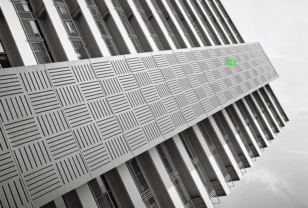
Urban100 ($\times 2$): img092 HR Bicubic VDSR [4] CARN-M [11] CARN [11] IMDN [29] PSNR/SSIM 19.15/0.6690 22.37/0.8185 22.54/0.8261 23.21/0.8410 23.72/0.8511 MADNet [54] AWSRN-M [53] LBNet [20] BSRN [61] FDIWN [24] Ours 22.89/0.8337 23.70/0.8510 24.05/0.8552 23.53/0.8498 23.84/0.8532 24.40/0.8625

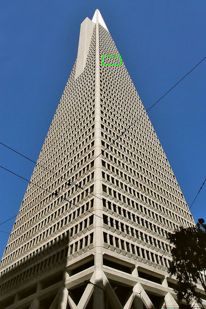
Urban100 ($\times 3$): img048 HR Bicubic VDSR [4] CARN-M [11] CARN [11] IMDN [29] PSNR/SSIM 19.59/0.7581 21.31/0.8550 21.97/0.8757 22.32/0.8842 22.36/0.8872 MADNet [54] AWSRN-M [53] LBNet [20] BSRN [61] FDIWN [24] Ours 22.15/0.8784 22.26/0.8860 22.84/0.8955 22.41/0.8871 22.48/0.8892 23.49/0.9100

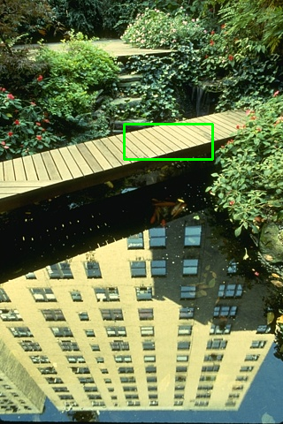
BSDS100 ($\times 4$): 148026 HR Bicubic VDSR [4] CARN-M [11] CARN [11] IMDN [29] PSNR/SSIM 20.75/0.5573 21.71/0.6578 21.94/0.6760 22.10/0.6883 22.13/0.6889 MADNet [54] AWSRN-M [53] LBNet [20] BSRN [61] FDIWN [24] Ours 22.04/0.6823 22.08/0.6880 22.24/0.6983 22.17/0.6930 22.14/0.6940 22.33/0.7055

Manga109 ($\times 3$): MomoyamaHaikagura HR Bicubic BSRN [61] IMDN [29] PSNR/SSIM 23.74/0.7034 25.92/0.8550 25.90/0.8534 AWSRN-M [53] LBNet [24] FDIWN [20] Ours 25.90/0.8534 25.66/0.8435 25.98/0.8557 26.16/0.8605 Manga109 ($\times 4$): TaiyouNiSmash HR Bicubic BSRN [61] IMDN [29] PSNR/SSIM 29.49/0.8712 35.90/0.9536 35.41/0.9499 AWSRN-M [53] LBNet [24] FDIWN [20] Ours 35.68/0.9513 36.08/0.9522 35.65/0.9508 36.50/0.9550

Figure 11: Visual comparison of FIWHN with other advanced SISR methods.

4.4 Comparisons with State-of-the-Art Methods

In this section, we perform an extensive comparison with state-of-the-art methods on the mainstream SR benchmark datasets. The quantitative comparison results for $\times 2$, $\times 3$, and $\times 4$ image SR are given in TABLE VII, where ”+” is the result of using self-ensemble. It can be clearly seen that our proposed FIWHN and FIWHN+ achieve the best and the second-best performance on almost all datasets. Moreover, by stacking limited computational resources, the number of parameters and the Multi-adds of our method is much lower than most of the methods. Meanwhile, compared to our conference version FDIWN [24], we have further improved the performance with only a small increase in computational cost. In particular, on Urban100 and Manga109 test sets, the performance gain is more than 0.3 dB on average for all three scale factors. These improvements demonstrate the effectiveness of our enhanced utilization of intermediate layer features through a wide residual mechanism and the necessity of using the Transformer to complement the global features of the CNN model.

In addition, we also compare our method with some advanced Transformer-based methods in TABLE VI. It can be clearly seen that the average performance of our method on several datasets is much better than those of ESRT [19], LBNet [20], CFIN [22], and roughly comparable to SwinIR [18]. However, it is worth noting that SwinIR additionally uses a pre-training strategy to enhance the model performance and uses a larger patch size for training, which is known to imply potentially better performance. And it has a substantially higher number of parameters and computations than our method. In terms of the difficulty of model promotion and deployment, our model has no major disadvantage in terms of training memory and inference time. The training of our model can be done on an NVIDIA RTX 2080Ti, and the inference speed is the second fastest among these methods. The smaller computation size is also an advantage of our FIWHN in deployment. All these experiments illustrate that our proposed FIWHN is a very competitive approach.

A qualitative comparison of our method with other methods is shown in Fig. 11. To make the comparisons more convincing, these comparison methods include the latest CNN-based methods and Transformer-based methods. And we not only give the visual comparison, but also the corresponding PSNR/SSIM values for each image. As can be seen in the figure, our method not only has higher PSNR values, but also outperforms other methods in terms of the visual quality of details on multiple validation sets, and can recover diverse texture details more accurately at all scales.

5 EFFECTIVENESS ON OTHER SISR TASKS

In this section, we describe the performance of FIWHN on face super-resolution and real-world image super-resolution. To further illustrate the effectiveness of our method, we also verify the beneficial effects of low-quality images after super-resolution on some downstream high-level tasks.

5.1 Face Image Super-Resolution

Dataset and implement details. We use CelebA [62] to train and Helen [63] to evaluate. We crop face images with 128$\times$128 pixels from the CelebA set to use as HR and then obtain LR images of the desired size by several downsampling. Face super-resolution methods such as Sparnet [52] are used for face reconstruction by encoding, feature extraction and decoding. The encoding and decoding processes are almost same for most methods, so we replace the feature extraction process within Sparnet’s framework with the model we need to perform comparisons.

TABLE VIII: Quantitative comparisons for SR on the CelebA and Helen test sets.

Methods	Scale	Params	$CelebA$				$Helen$
			PSRN${\uparrow}$	SSIM${\uparrow}$	VIF${\uparrow}$	LPIPS${\downarrow}$	PSNR${\uparrow}$	SSIM${\uparrow}$	VIF${\uparrow}$	LPIPS${\downarrow}$
Bicubic	$\times 8$	-	23.61	0.6779	0.1821	0.4899	22.95	0.6762	0.1745	0.4912
SAN [50]		16.00M	27.43	0.7826	0.4553	0.2080	25.46	0.7360	0.4029	0.3260
RCAN [37]		15.70M	27.45	0.7824	0.4618	0.2205	25.50	0.7383	0.4049	0.3437
HAN [51]		16.20M	27.47	0.7838	0.4673	0.2087	25.40	0.7347	0.4074	0.3274
FSRNet [64]		27.50M	27.05	0.7714	0.3852	0.2127	25.45	0.7364	0.3482	0.3090
SPARNet [52]		16.59M	27.73	0.7949	0.4505	0.1995	26.43	0.7839	0.4262	0.2674
IMDN [29]		12.70M	27.97	0.7998	0.4669	0.1928	26.66	0.7911	0.4363	0.2497
FDIWN [24]		11.10M	27.98	0.8002	0.4639	0.1893	26.73	0.7932	0.4451	0.2413
[3pt/3pt] FIWHN (ours)		10.50M	28.10	0.8056	0.4720	0.1804	26.84	0.8004	0.4514	0.2297

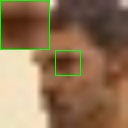
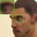
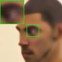
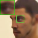
PSNR/SSIM	26.47/0.7758	30.39/0.8275	30.40/0.8275	30.44/0.8290	31.10/0.8410	31.41/0.8472	31.35/0.8496	31.48/0.8561
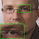
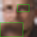
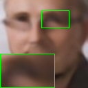
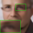
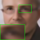
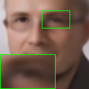
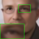
PSNR/SSIM	25.15/0.7009	26.31/0.7359	26.17/0.7403	26.21/0.7394	27.65/0.8015	27.77/0.8053	27.89/0.8030	28.23/0.81774
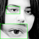
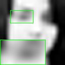
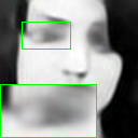
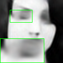
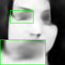
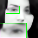
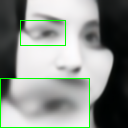
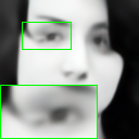
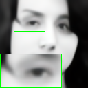
PSNR/SSIM	21.44/0.6419	23.38/0.7392	23.15/0.7313	23.60/0.7481	23.29/0.7331	24.28/0.7847	24.68/0.7857	25.03/0.7974
HR	Bicubic	SAN [50]	RCAN [37]	HAN [51]	SPARNet [52]	IMDN [29]	FDIWN [24]	Ours

Figure 12: Visual comparisons for $\times 8$ SR on the CelebA test set and Helen test set.

Comparison results. For fair comparisons, we also list some general image super-resolution approaches. TABLE VIII shows the obtained quantitative comparison results in terms of PSNR, SSIM, LPIPS, and VIF. From the table, we can see that our approach effectively improves the performance while significantly reducing the computational cost compared to the face super-resolution approaches [64, 52]. The qualitative visual results of $\times 8$ SR on face test set images are illustrated in Fig. 12. Since the pupil of the human eye is crucial to the face recognition task, we deliberately selected features around the eye region of the face for comparison. As can be seen from the figure, some methods cannot even recover the contour of the human eye. Although others can recover the orbital contour, their reconstruction details are still inaccurate compared to HR. Compared to these methods, our method tends to recover more accurate human eye contours and pupil positions. This further demonstrates the effectiveness of our FIWHN.

As downstream tasks after face super-resolution, face detection and face recognition tasks play an important role in security surveillance and other fields. We use YuNet [65] as a face detection model and SFace [66] as a face recognition model, where SFace is working on face recognition based on the bounding box of the face detected by YuNet on super-resolved faces. We still use CelebA and Helen as the validation sets for face detection and recognition. As can be seen in TABLE V, the low-quality Bicubic is detrimental to face recognition work, with only 19.8$\%$ recognition rate on the CelebA dataset. The super-resolution reconstruction methods can significantly improve face recognition rates. And among all of the compared advanced super-resolution methods, our method achieves the best results in face recognition and detection tasks, infinitely close to the results achieved by HR faces. Compared to the conference version, our method can improve the recognition rate on each of the two datasets with a smaller number of parameters.

5.2 Real-World Image Super-Resolution

Dataset and implement details. We use RealSR [67] as our training and testing sets, where HR and LR are obtained by acquiring data in the same scene, using the same camera with different focal lengths. Compared with the DIV2K dataset, its degradation model is more complex, and the degradation kernel is spatially variable. It is worth noting that the dimensions of LR and HR in this dataset are already aligned, so all methods remove the upsampling operation at the back end of the model when performing super-resolution. Therefore, the number of parameters and the calculations amount for all methods are basically the same as in TABLE VII. However, the requirement for the model to align pixels during image recovery is increased due to the pixel drift, scale factor changes, and other issues brought about by adjusting the focal length. To alleviate the extra difficulty caused by pixel alignment, most methods adopt the strategy of cutting image patches into large patches when cutting them to feed into the network for training. Such an operation can alleviate the difficulty caused by the edge information between too many patches not communicating with each other for aligning pixels. These methods set the image patch to 128$\times$128 during training, while we can only set the patch of FDIWN and FIWHN to 64$\times$64 during training due to the higher training memory associated with a larger patch size. Therefore, our FIWHN can be trained on one NVIDIA RTX 2080Ti GPU, while other methods cannot be trained even on two NVIDIA RTX 2080Ti GPUs.

TABLE IX: Comparison with other advance SISR model on RealSR dataset [67].

Scale	Bicubic	SRCNN [3]	VDSR [3]	SRResNet [68]	IMDN [29]	ESRT [19]	FDIWN [24]	FIWHN(ours)
	PSNR / SSIM	PSNR / SSIM	PSNR / SSIM	PSNR / SSIM	PSNR / SSIM	PSNR / SSIM	PSNR / SSIM	PSNR / SSIM
$\times 2$	32.61 / 0.907	33.40 / 0.916	33.64 / 0.917	33.69 / 0.919	33.85 / 0.923	33.92 / 0.924	33.68/0.9242	33.96 / 0.927
$\times 3$	29.34 / 0.841	29.96 / 0.845	30.14 / 0.856	30.18 / 0.859	30.29 / 0.857	30.38 / 0.857	30.38 / 0.857	30.57 / 0.862
$\times 4$	27.99 / 0.806	28.44 / 0.801	28.63 / 0.821	28.67 / 0.824	28.68 / 0.815	28.78 / 0.815	28.70 / 0.815	28.82 / 0.828

RealSR ($\times 2$): Canon010 HR LR PSNR/SSIM 29.23/0.9102 FDIWN [24] Ours 32.24/0.9505 32.50/0.9517 RealSR ($\times 3$): Nikon009 HR LR PSNR/SSIM 29.33/0.8155 FDIWN [24] Ours 31.05/0.8740 31.45/0.8802 RealSR ($\times 4$): Nikon006 HR LR PSNR/SSIM 24.03/0.7896 FDIWN [24] Ours 24.77/0.8264 24.86/0.8327

Figure 13: Visual comparison on RealSR dataset (Including Nikon and Canon).

Comparison results. In a training situation where our method is at a disadvantage, the final quantitative comparison results are given in TABLE IX. Our method still achieves the best results at all scales, especially at the scale factor of $\times 3$, where our method outperforms the second-best ESRT method with a PSNR value of 0.19 dB. Next, we give visual comparisons. The detailed comparisons in Fig. 13 show that our FIWHN can recover more textural details than that of the conference version FDIWN, and the recovery results are closer to the HR image. To further validate the effectiveness of FIWHN, we evaluate the benefits of our approach for street image semantic segmentation tasks. To this end, we first downsample the images from commonly used validation set of CamVid [69] dataset and then use the SR methods to recover the high-quality images. Finally, segmenting them with recently published real-time segmentation method FBSNet [70]. As can be seen in Fig. 14, the segmentation results of the recovered images by our method is closer to the ground truth. Specifically, for the segmented details, such as the utility poles, our FIWHN clearly outperforms simple Bicubic and our conference version FDIWN.

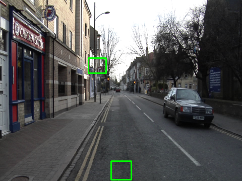
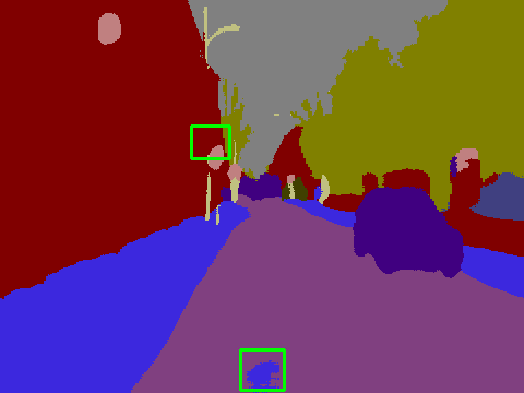
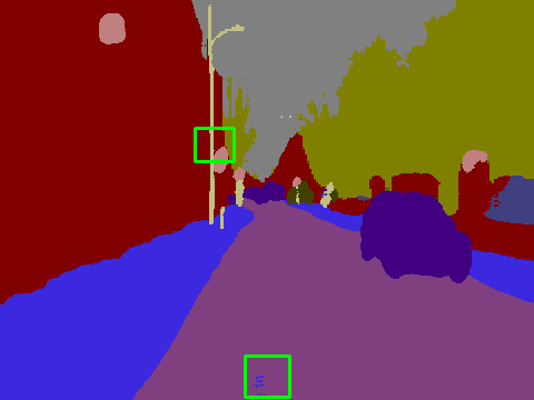
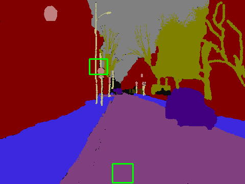
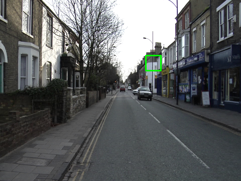
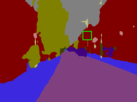
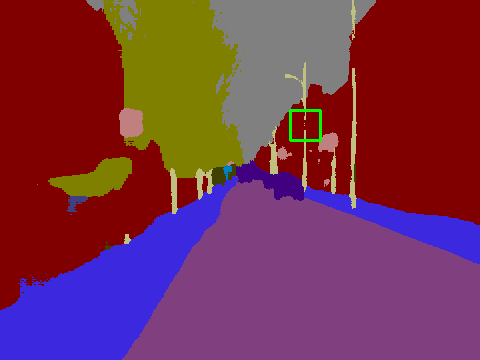
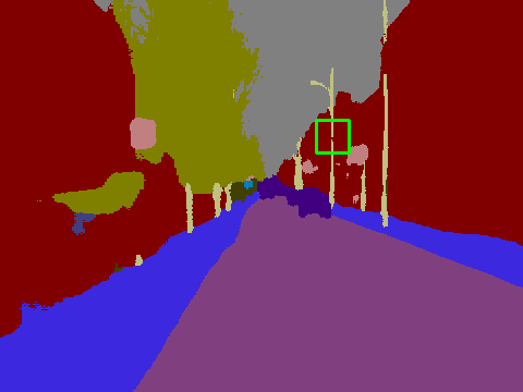
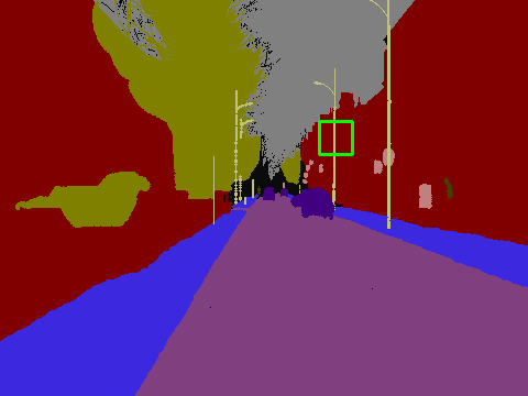
Street View	Bicubic	FDIWN [24]	Ours	Ground Truth

Figure 14: Comparison of image segmentation results ($\times 2$ SR).

6 CONCLUSIONS

In this work, we have carefully designed a Feature Interaction Weighted Hybrid Network (FIWHN) to support efficient super-resolution tasks. FIWHN is composed of groups of WDIBs that are blended, fused， and weighted. WDIBs use combinatorial coefficient learning to connect wide residual weighted units that can mitigate the loss of intermediate layers to induce different combinatorial structures. And it allows features with different refinement levels to exploit different levels of information by jump joining and fusion. Subsequently, a more enhanced model generalization architecture is designed by introducing Transformer to prompt the model to capture global features. Subsequently, we extend FIWHN to other SR tasks, including face SR and real-world SR. Meanwhile, the effectiveness of our method is verified on many downstream tasks, including face detection, face recognition, and semantic segmentation. All of these experiments have demonstrated that our proposed method can perform super-resolution tasks more efficiently.

References

- [1] G. Gao, Y. Yu, H. Lu, J. Yang, and D. Yue, “Context-patch representation learning with adaptive neighbor embedding for robust face image super-resolution,” IEEE Transactions on Multimedia, 2022.
- [2] K. C. Chan, X. Xu, X. Wang, J. Gu, and C. C. Loy, “Glean: Generative latent bank for image super-resolution and beyond,” IEEE Transactions on Pattern Analysis and Machine Intelligence, 2022.
- [3] C. Dong, C. C. Loy, K. He, and X. Tang, “Image super-resolution using deep convolutional networks,” IEEE Transactions on Pattern Analysis and Machine Intelligence, vol. 38, no. 2, pp. 295–307, 2015.
- [4] J. Kim, J. K. Lee, and K. M. Lee, “Accurate image super-resolution using very deep convolutional networks,” in Proceedings of the IEEE Conference on Computer Vision and Pattern Recognition, 2016, pp. 1646–1654.
- [5] B. Lim, S. Son, H. Kim, S. Nah, and K. Mu Lee, “Enhanced deep residual networks for single image super-resolution,” in Proceedings of the IEEE Conference on Computer Vision and Pattern Recognition Workshops, 2017, pp. 136–144.
- [6] Y. Zhang, Y. Tian, Y. Kong, B. Zhong, and Y. Fu, “Residual dense network for image super-resolution,” in Proceedings of the IEEE Conference on Computer Vision and Pattern Recognition, 2018, pp. 2472–2481.
- [7] W.-S. Lai, J.-B. Huang, N. Ahuja, and M.-H. Yang, “Fast and accurate image super-resolution with deep laplacian pyramid networks,” IEEE Transactions on Pattern Analysis and Machine Intelligence, vol. 41, no. 11, pp. 2599–2613, 2018.
- [8] J. Li, F. Fang, K. Mei, and G. Zhang, “Multi-scale residual network for image super-resolution,” in Proceedings of the European conference on computer vision (ECCV), 2018, pp. 517–532.
- [9] J. Li, F. Fang, J. Li, K. Mei, and G. Zhang, “Mdcn: Multi-scale dense cross network for image super-resolution,” IEEE Transactions on Circuits and Systems for Video Technology, vol. 31, no. 7, pp. 2547–2561, 2020.
- [10] X. Chu, B. Zhang, H. Ma, R. Xu, and Q. Li, “Fast, accurate and lightweight super-resolution with neural architecture search,” in Proceedings of the International Conference on Pattern Recognition (ICPR). IEEE, 2021, pp. 59–64.
- [11] N. Ahn, B. Kang, and K.-A. Sohn, “Fast, accurate, and lightweight super-resolution with cascading residual network,” in Proceedings of the European Conference on Computer Vision (ECCV), 2018, pp. 252–268.
- [12] Z. Wang, G. Gao, J. Li, Y. Yu, and H. Lu, “Lightweight image super-resolution with multi-scale feature interaction network,” in Proceedings of the International Conference on Multimedia and Expo (ICME), 2021, pp. 1–6.
- [13] M. Sandler, A. Howard, M. Zhu, A. Zhmoginov, and L.-C. Chen, “Mobilenetv2: Inverted residuals and linear bottlenecks,” in Proceedings of the IEEE Conference on Computer Vision and Pattern Recognition, 2018, pp. 4510–4520.
- [14] B. Li and X. Gao, “Lattice structure for regular linear phase paraunitary filter bank with odd decimation factor,” IEEE Signal Processing Letters, vol. 21, no. 1, pp. 14–17, 2013.
- [15] X. Luo, Y. Qu, Y. Xie, Y. Zhang, C. Li, and Y. Fu, “Lattice network for lightweight image restoration,” IEEE Transactions on Pattern Analysis and Machine Intelligence, 2022.
- [16] S. W. Zamir, A. Arora, S. Khan, M. Hayat, F. S. Khan, and M.-H. Yang, “Restormer: Efficient transformer for high-resolution image restoration,” in Proceedings of the IEEE Conference on Computer Vision and Pattern Recognition, 2022, pp. 5728–5739.
- [17] R. Yu, D. Du, R. LaLonde, D. Davila, C. Funk, A. Hoogs, and B. Clipp, “Cascade transformers for end-to-end person search,” in Proceedings of the IEEE Conference on Computer Vision and Pattern Recognition, June 2022, pp. 7267–7276.
- [18] J. Liang, J. Cao, G. Sun, K. Zhang, L. Van Gool, and R. Timofte, “Swinir: Image restoration using swin transformer,” in Proceedings of the IEEE/CVF International Conference on Computer Vision (ICCV) Workshops, 2021, pp. 1833–1844.
- [19] Z. Lu, J. Li, H. Liu, C. Huang, L. Zhang, and T. Zeng, “Transformer for single image super-resolution,” in Proceedings of the IEEE/CVF Conference on Computer Vision and Pattern Recognition (CVPR) Workshops, 2022, pp. 457–466.
- [20] G. Gao, Z. Wang, J. Li, W. Li, Y. Yu, and T. Zeng, “Lightweight bimodal network for single-image super-resolution via symmetric cnn and recursive transformer,” in Proceedings of the International Joint Conference on Artificial Intelligence, 2022, pp. 661–669.
- [21] X. Zhang, H. Zeng, S. Guo, and L. Zhang, “Efficient long-range attention network for image super-resolution,” arXiv preprint arXiv:2203.06697, 2022.
- [22] W. Li, J. Li, G. Gao, J. Zhou, J. Yang, and G.-J. Qi, “Cross-receptive focused inference network for lightweight image super-resolution,” arXiv preprint arXiv:2207.02796, 2022.
- [23] Y. Chen, X. Dai, D. Chen, M. Liu, X. Dong, L. Yuan, and Z. Liu, “Mobile-former: Bridging mobilenet and transformer,” in Proceedings of the IEEE/CVF Conference on Computer Vision and Pattern Recognition, 2022, pp. 5270–5279.
- [24] G. Gao, W. Li, J. Li, F. Wu, H. Lu, and Y. Yu, “Feature distillation interaction weighting network for lightweight image super-resolution,” in Proceedings of the AAAI Conference on Artificial Intelligence, vol. 36, no. 1, 2022, pp. 661–669.
- [25] Y. Li, J. Cao, Z. Li, S. Oh, and N. Komuro, “Lightweight single image super-resolution with dense connection distillation network,” ACM Transactions on Multimedia Computing, Communications, and Applications (TOMM), vol. 17, no. 1s, pp. 1–17, 2021.
- [26] X. Zhang, H. Zeng, and L. Zhang, “Edge-oriented convolution block for real-time super resolution on mobile devices,” in Proceedings of the ACM International Conference on Multimedia, 2021, pp. 4034–4043.
- [27] D. Zhang, C. Li, N. Xie, G. Wang, and J. Shao, “Pffn: Progressive feature fusion network for lightweight image super-resolution,” in Proceedings of the ACM International Conference on Multimedia, 2021, pp. 3682–3690.
- [28] X. Zhu, K. Guo, S. Ren, B. Hu, M. Hu, and H. Fang, “Lightweight image super-resolution with expectation-maximization attention mechanism,” IEEE Transactions on Circuits and Systems for Video Technology, vol. 32, no. 3, pp. 1273–1284, 2022.
- [29] Z. Hui, X. Gao, Y. Yang, and X. Wang, “Lightweight image super-resolution with information multi-distillation network,” in Proceedings of the ACM International Conference on Multimedia, 2019, pp. 2024–2032.
- [30] X. Luo, Y. Xie, Y. Zhang, Y. Qu, C. Li, and Y. Fu, “Latticenet: Towards lightweight image super-resolution with lattice block,” in Proceedings of the European Conference on Computer Vision (ECCV), 2020, pp. 272–289.
- [31] H. Li, C. Yan, S. Lin, X. Zheng, B. Zhang, F. Yang, and R. Ji, “Pams: Quantized super-resolution via parameterized max scale,” in Proceedings of the European Conference on Computer Vision. Springer, 2020, pp. 564–580.
- [32] W. Lee, J. Lee, D. Kim, and B. Ham, “Learning with privileged information for efficient image super-resolution,” in Proceedings of the European Conference on Computer Vision. Springer, 2020, pp. 465–482.
- [33] Y. Tai, J. Yang, and X. Liu, “Image super-resolution via deep recursive residual network,” in Proceedings of the IEEE Conference on Computer Vision and Pattern Recognition, 2017, pp. 3147–3155.
- [34] J.-H. Choi, J.-H. Kim, M. Cheon, and J.-S. Lee, “Lightweight and efficient image super-resolution with block state-based recursive network,” arXiv preprint arXiv:1811.12546, 2018.
- [35] Z. Hui, X. Wang, and X. Gao, “Fast and accurate single image super-resolution via information distillation network,” in Proceedings of the IEEE/CVF Conference on Computer Vision and Pattern Recognition (CVPR), 2018, pp. 723–731.
- [36] X. Jiang, N. Wang, J. Xin, X. Xia, X. Yang, and X. Gao, “Learning lightweight super-resolution networks with weight pruning,” Neural Networks, vol. 144, pp. 21–32, 2021.
- [37] Y. Zhang, K. Li, K. Li, L. Wang, B. Zhong, and Y. Fu, “Image super-resolution using very deep residual channel attention networks,” in Proceedings of the European conference on computer vision (ECCV), 2018, pp. 286–301.
- [38] K. He, X. Zhang, S. Ren, and J. Sun, “Deep residual learning for image recognition,” in Proceedings of the IEEE Conference on Computer Vision and Pattern Recognition, 2016, pp. 770–778.
- [39] J. Yu, Y. Fan, J. Yang, N. Xu, Z. Wang, X. Wang, and T. Huang, “Wide activation for efficient and accurate image super-resolution,” arXiv preprint arXiv:1808.08718, 2018.
- [40] Z. Liu, Y. Lin, Y. Cao, H. Hu, Y. Wei, Z. Zhang, S. Lin, and B. Guo, “Swin transformer: Hierarchical vision transformer using shifted windows,” in Proceedings of the IEEE/CVF International Conference on Computer Vision, 2021, pp. 10 012–10 022.
- [41] Y. Wang, T. Lu, Y. Zhang, J. Jiang, J. Wang, Z. Wang, and J. Ma, “Tanet: A new paradigm for global face super-resolution via transformer-cnn aggregation network,” arXiv preprint arXiv:2109.08174, 2021.
- [42] R. Timofte, E. Agustsson, L. Van Gool, M.-H. Yang, and L. Zhang, “Ntire 2017 challenge on single image super-resolution: Methods and results,” in Proceedings of the IEEE/CVF Conference on Computer Vision and Pattern Recognition Workshops, 2017, pp. 114–125.
- [43] M. Bevilacqua, A. Roumy, C. Guillemot, and M. L. Alberi-Morel, “Low-complexity single-image super-resolution based on nonnegative neighbor embedding,” in Proceedings of the British Machine Vision Conference (BMVC), 2012, pp. 135.1–135.10.
- [44] R. Zeyde, M. Elad, and M. Protter, “On single image scale-up using sparse-representations,” in Proceedings of the International Conference on Curves and Surfaces (ICCS), 2010, pp. 711–730.
- [45] D. Martin, C. Fowlkes, D. Tal, and J. Malik, “A database of human segmented natural images and its application to evaluating segmentation algorithms and measuring ecological statistics,” in Proceedings of the IEEE International Conference on Computer Vision, 2001, pp. 416–423.
- [46] J.-B. Huang, A. Singh, and N. Ahuja, “Single image super-resolution from transformed self-exemplars,” in Proceedings of the IEEE/CVF Conference on Computer Vision and Pattern Recognition, 2015, pp. 5197–5206.
- [47] Y. Matsui, K. Ito, Y. Aramaki, A. Fujimoto, T. Ogawa, T. Yamasaki, and K. Aizawa, “Sketch-based manga retrieval using manga109 dataset,” Multimedia Tools and Applications, vol. 76, no. 20, pp. 21 811–21 838, 2017.
- [48] T. Salimans and D. P. Kingma, “Weight normalization: A simple reparameterization to accelerate training of deep neural networks,” Advances in neural information processing systems, vol. 29, 2016.
- [49] J. Liu, J. Tang, and G. Wu, “Residual feature distillation network for lightweight image super-resolution,” in Proceedings of the European Conference on Computer Vision (ECCV), 2020, pp. 41–55.
- [50] T. Dai, J. Cai, Y. Zhang, S.-T. Xia, and L. Zhang, “Second-order attention network for single image super-resolution,” in Proceedings of the IEEE/CVF Conference on Computer Vision and Pattern Recognition, 2019, pp. 11 065–11 074.
- [51] B. Niu, W. Wen, W. Ren, X. Zhang, L. Yang, S. Wang, K. Zhang, X. Cao, and H. Shen, “Single image super-resolution via a holistic attention network,” in Proceedings of the European Conference on Computer Vision, 2020, pp. 191–207.
- [52] C. Chen, D. Gong, H. Wang, Z. Li, and K.-Y. K. Wong, “Learning spatial attention for face super-resolution,” IEEE Transactions on Image Processing, vol. 30, pp. 1219–1231, 2021.
- [53] C. Wang, Z. Li, and J. Shi, “Lightweight image super-resolution with adaptive weighted learning network,” arXiv preprint arXiv:1904.02358, 2019.
- [54] R. Lan, L. Sun, Z. Liu, H. Lu, C. Pang, and X. Luo, “Madnet: a fast and lightweight network for single-image super resolution,” IEEE Transactions on Cybernetics, vol. 51, no. 3, pp. 1443–1453, 2020.
- [55] A. Muqeet, J. Hwang, S. Yang, J. Kang, Y. Kim, and S.-H. Bae, “Multi-attention based ultra lightweight image super-resolution,” in Proceedings of the European Conference on Computer Vision (ECCV), 2020, pp. 103–118.
- [56] W. Li, K. Zhou, L. Qi, N. Jiang, J. Lu, and J. Jia, “Lapar: Linearly-assembled pixel-adaptive regression network for single image super-resolution and beyond,” Advances in Neural Information Processing Systems, vol. 33, pp. 20 343–20 355, 2020.
- [57] X. Zhang, P. Gao, S. Liu, K. Zhao, G. Li, L. Yin, and C. W. Chen, “Accurate and efficient image super-resolution via global-local adjusting dense network,” IEEE Transactions on Multimedia, vol. 23, pp. 1924–1937, 2021.
- [58] L. Wang, X. Dong, Y. Wang, X. Ying, Z. Lin, W. An, and Y. Guo, “Exploring sparsity in image super-resolution for efficient inference,” in Proceedings of the IEEE/CVF Conference on Computer Vision and Pattern Recognition (CVPR), 2021, pp. 4917–4926.
- [59] K. Park, J. W. Soh, and N. I. Cho, “Dynamic residual self-attention network for lightweight single image super-resolution,” IEEE Transactions on Multimedia, 2021.
- [60] Z. Du, D. Liu, J. Liu, J. Tang, G. Wu, and L. Fu, “Fast and memory-efficient network towards efficient image super-resolution,” in Proceedings of the IEEE Conference on Computer Vision and Pattern Recognition, 2022, pp. 853–862.
- [61] Z. Li, Y. Liu, X. Chen, H. Cai, J. Gu, Y. Qiao, and C. Dong, “Blueprint separable residual network for efficient image super-resolution,” in Proceedings of the IEEE/CVF Conference on Computer Vision and Pattern Recognition, 2022, pp. 833–843.
- [62] Z. Liu, P. Luo, X. Wang, and X. Tang, “Deep learning face attributes in the wild,” in Proceedings of the IEEE International Conference on Computer Vision, 2015, pp. 3730–3738.
- [63] V. Le, J. Brandt, Z. Lin, L. Bourdev, and T. S. Huang, “Interactive facial feature localization,” in Proceedings of the European Conference on Computer Vision. Springer, 2012, pp. 679–692.
- [64] Y. Chen, Y. Tai, X. Liu, C. Shen, and J. Yang, “Fsrnet: End-to-end learning face super-resolution with facial priors,” in Proceedings of the IEEE Conference on Computer Vision and Pattern Recognition, 2018, pp. 2492–2501.
- [65] Y. Feng, S. Yu, H. Peng, Y. ran Li, and J. Zhang, “Detect faces efficiently: A survey and evaluations,” IEEE Transactions on Biometrics, Behavior, and Identity Science, 2021.
- [66] Y. Zhong, W. Deng, J. Hu, D. Zhao, X. Li, and D. Wen, “Sface: Sigmoid-constrained hypersphere loss for robust face recognition,” IEEE Transactions on Image Processing, vol. 30, pp. 2587–2598, 2021.
- [67] J. Cai, H. Zeng, H. Yong, Z. Cao, and L. Zhang, “Toward real-world single image super-resolution: A new benchmark and a new model,” in Proceedings of the IEEE International Conference on Computer Vision, 2019, pp. 3086–3095.
- [68] C. Ledig, L. Theis, F. Huszár, J. Caballero, A. Cunningham, A. Acosta, A. Aitken, A. Tejani, J. Totz, Z. Wang et al., “Photo-realistic single image super-resolution using a generative adversarial network,” in Proceedings of the IEEE Conference on Computer Vision and Pattern Recognition, 2017, pp. 4681–4690.
- [69] G. J. Brostow, J. Shotton, J. Fauqueur, and R. Cipolla, “Segmentation and recognition using structure from motion point clouds,” in Proceedings of the European Conference on Computer Vision. Springer, 2008, pp. 44–57.
- [70] G. Gao, G. Xu, J. Li, Y. Yu, H. Lu, and J. Yang, “Fbsnet: A fast bilateral symmetrical network for real-time semantic segmentation,” IEEE Transactions on Multimedia, 2022.