A Data-Adaptive Prior for Bayesian Learning
of Kernels in Operators

Abstract

Kernels are efficient in representing nonlocal dependence and they are widely used to design operators between function spaces. Thus, learning kernels in operators from data is an inverse problem of general interest. Due to the nonlocal dependence, the inverse problem can be severely ill-posed with a data-dependent singular inversion operator. The Bayesian approach overcomes the ill-posedness through a non-degenerate prior. However, a fixed non-degenerate prior leads to a divergent posterior mean when the observation noise becomes small, if the data induces a perturbation in the eigenspace of zero eigenvalues of the inversion operator. We introduce a data-adaptive prior to achieve a stable posterior whose mean always has a small noise limit. The data-adaptive prior’s covariance is the inversion operator with a hyper-parameter selected adaptive to data by the L-curve method. Furthermore, we provide a detailed analysis on the computational practice of the data-adaptive prior, and demonstrate it on Toeplitz matrices and integral operators. Numerical tests show that a fixed prior can lead to a divergent posterior mean in the presence of any of the four types of errors: discretization error, model error, partial observation and wrong noise assumption. In contrast, the data-adaptive prior always attains posterior means with small noise limits.

Keywords: Data-adaptive prior, kernels in operators, linear Bayesian inverse problem,
RKHS, Tikhonov regularization

2020 Mathematics Subject Classification: 62F15, 47A52, 47B32

1 Introduction

Kernels are efficient in representing nonlocal or long-range dependence and interaction between high- or infinite-dimensional variables. They are widely used to design operators between function spaces, with numerous applications in machine learning such as kernel methods (e.g., [5, 9, 13, 26, 50, 45]) and operator learning (e.g., [28, 41]), in partial differential equations (PDEs) and stochastic processes such as nonlocal and fractional diffusions (e.g., [6, 17, 19, 55, 56]), and in multi-agent systems (e.g., [7, 37, 39, 44]).

The inverse problem of learning kernels in operators from data is an integral part of these applications. Most of the kernels are user-specified with a few hyper-parameters tuned to fit data. But the increasing complexity of kernels in applications, particularly those in PDEs and multi-agent systems, calls for general kernels to be learned from data.

A starting point is to learn the kernel via regression when the operator depends linearly on the kernel. However, due to the nonlocal dependence, the inverse problem is often severely ill-posed with an inversion operator that is singular (or low-rank) and data-dependent ([29, 35]). This inversion operator is the covariance matrix of the likelihood distribution when the kernel is finite-dimensional, and it is the second order derivative of the loss functional in a variational approach.

The Bayesian approach overcomes the ill-posedness by introducing a prior, so that the posterior is stable under perturbations in the observation noise (e.g., [14, 27, 51]). Since little prior information is available about the kernel, it is common to use a non-degenerate prior to ensure the well-posedness of the posterior.

However, we show that a fixed non-degenerate prior has the risk of a catastrophic error: it leads to a divergent posterior mean as the observation noise decreases to zero, if the data induces a perturbation in the eigenspace of zero eigenvalues of the inversion operator (see Theorem 3.2). Such a perturbation can be caused by any of the four types of errors in data or computation: (i) discretization error, (ii) model error, (iii) partial observations, and (iv) wrong noise assumption. In particular, both the inversion operator and the perturbation are data-dependent.

We solve the issue by a data-adaptive prior. The data-adaptive prior’s covariance is the inversion operator with a hyper-parameter selected adaptive to data. We prove that it leads to a stable posterior whose mean always has a small noise limit, and the small noise limit converges to the identifiable parts of the true kernel (in Theorem 4.2). Additionally, the data-adaptive prior can improve the quality of the posterior in two aspects: (i) reducing the expected mean square error of the MAP estimator; and (ii) reducing the uncertainty in the posterior in terms of the trace of the posterior covariance (see Section 4.2).

Furthermore, we provide a detailed analysis on the computational practice of the data-adaptive prior. We select the hyper-parameter by the widely-used L-curve method by [24]. Numerical tests on the Toeplitz matrices and integral operators show that while a fixed non-degenerate prior leads to divergent posterior means, the data-adaptive prior always attains posterior means with small noise limits (see Section 5).

The outline of this study is as follows. We review related work in Section 1.1. Section 2 introduces the inverse problem of learning kernels in operators, and it reviews the variational approach and a closely related regularization method. In particular, it presents the mathematical setup of this study, and shows the ill-posedness of the inverse problem. The ill-posedness leads onto Section 3 where we introduce the Bayesian approach and show the issue of a fixed non-degenerate prior. To solve the issue, we introduce a data-adaptive prior in Section 4, and analyze its advantage. Section 5 discusses the data-adaptive prior in computational practice and demonstrates the advantage of the data-adaptive prior in numerical tests on Toeplitz matrices and integral operators. Finally, in Section 6 we conclude our findings and provide some future research directions related to this work. The Appendix includes the proofs and some computational details.

1.1 Related work

Bayesian inverse problems.

We study the selection of a prior for Bayesian linear inverse problems when the likelihood has a deficient ranked covariance matrix. Thus, the focus is different from the studies of Bayesian inverse problems that focus on efficient sampling of the posterior [14, 27, 49, 51] when the prior is pre-specified, even though the low-rank property has been utilized for fast approximation of the posterior mean in [10, 49]. Importantly, we re-discover the well-known Zellner’s g-prior [1, 4, 58] when the kernel is finite-dimensional and the basis functions are orthonormal in the function space of learning.

Variational approach and regularization.

The Bayesian approach is closely related to the variational approach and Tikhonov/ridge regularization methods. The likelihood function provides a loss function in a variational approach, and the prior often provides a regularization norm (also called a penalty term). Various regularization terms have been studied, including the widely-used Euclidean norm in the classical Tikhonov regularization (see e.g., [21, 23, 24, 53]), the RKHS norm with an ad hoc reproducing kernel (see e.g., [9, 3]), the total variation norm in the Rudin-Osher-Fatemi method in [47], the $L^{1}$ norm in LASSO (see e.g., [52]), and the data-adaptive RKHS norm in [35, 36]. In comparison, relatively few priors are studied in the Bayesian approach. The prior is often assumed to be known, or assumed to be a non-degenerate measure when there is little prior information. This study shows the advantage of a data-adaptive prior coming from the regularization with the data-adaptive RKHS norm.

Kernel methods and operator learning.

This study focuses on learning the kernels, not the operators. Thus, our focus differs from the focus of the widely-used kernel methods (see e.g.,[5, 9, 13, 26, 45, 50, 57]) and the operator learning (see e.g., [15, 16, 28, 34, 40, 41]). These methods aim to approximate the operator matching the input and output, not to identify the kernel in the operator.

Learning interacting kernels and nonlocal kernels.

The learning of kernels in operators has been studied in the context of identifying the interaction kernels in interacting particle systems (e.g., [20, 25, 18, 30, 33, 37, 39, 38, 42, 43, 54]) and the nonlocal kernels in homogenization of PDEs (e.g., [35, 55, 56]). This study is the first to analyze the selection of a prior in a Bayesian approach.

2 The learning of kernels in operators

This section introduces the inverse problem of learning kernels in operators. It presents the mathematical setup of this study: the function space of learning, the inversion operator, and the function space of identifiability.

2.1 Learning kernels in operators

We consider the inverse problem of identifying kernels in operators from data. That is, given data

$$\mathcal{D}=\{(u^{k},f^{k})\}_{k=1}^{N},\quad(u^{k},f^{k})\in\mathbb{X}\times\mathbb{Y},$$ (2.1)

where $\mathbb{X}$ is a Banach space and $\mathbb{Y}$ is a Hilbert space, our goal is to find a kernel function $\phi$ in an operator $R_{\phi}:\mathbb{X}\to\mathbb{Y}$ so that $R_{\phi}$ best fits the data pairs $\{(u^{k},f^{k})\}_{k=1}^{N}$ in the form

$$R_{\phi}[u]+\eta+\xi=f,$$ (2.2)

where the measurement noise $\eta$ is a $\mathbb{Y}$-valued white noise in the sense that $\mathbb{E}[\langle{\eta,f}\rangle_{\mathbb{Y}}^{2}]=\sigma_{\eta}^{2}\langle{f,f}\rangle_{\mathbb{Y}}$ for any $f\in\mathbb{Y}$. Here $\xi$, which we call model error, represents the unknown errors such as model error or computational error due to incomplete data, and it may depend on the input data $u$.

The operator $R_{\phi}$ can be either linear or nonlinear in $u$, but it depends linearly on $\phi$:

$$R_{c_{1}\phi_{1}+c_{2}\phi_{2}}=c_{1}R_{\phi_{1}}+c_{2}R_{\phi_{2}},$$ (2.3)

for any $c_{1},c_{2}\in\mathbb{R}$ and for $\phi_{1},\phi_{2}$ such that the operators $R_{\phi_{1}}$ and $R_{\phi_{2}}$ are well-defined. We focus on operators that depend non-locally on their kernels in the form

$$R_{\phi}[u](y)=\int_{\Omega}\phi(y-x)g[u](x,y)\mu(dx),\quad\forall y\in\Omega,$$ (2.4)

where $(\Omega,\mu)$ is a measure space that can be either a domain in the Euclidean space with the Lebesgue measure or a discrete set with a counting measure. A generalization to bivariate kernels $\phi(x,y):\Omega_{x}\times\Omega_{y}\to\mathbb{R}$ will be studied in a future work.

Such operators are widely seen in PDEs, matrix operators, and image processing. Examples include the Toeplitz matrix, the integral operators, and nonlocal operators. In these examples, the model error can come from homogenization or approximation of the integrals in the operators.

Example 2.1 (Kernels in Toeplitz matrices).

Consider the estimation of the kernel $\phi$ in the Toeplitz matrix $R_{\phi}\in\mathbb{R}^{n\times n}$, i.e., $R_{\phi}(i,j)=\phi(i-j)$ for all $1\leq i,j\leq n$, from measurement data $\{(u^{k},f^{k})\in\mathbb{R}^{n}\times\mathbb{R}^{n}\}_{k=1}^{N}$ by fitting the data to the model

$$R_{\phi}u+\eta+\xi(u)=f,\quad\eta\sim\mathcal{N}(0,\sigma_{\eta}^{2}I_{n}),\quad\mathbb{X}=\mathbb{Y}=\mathbb{R}^{n},$$ (2.5)

where $\xi(u)$ represents unknown model error. We can write the Toeplitz matrix as an integral operator in the form of (2.4) with $\Omega=\{1,2,\ldots,n\}$, $g[u](x,y)=u(y)$, and $\mu$ being a uniform discrete measure on $\Omega$. The kernel is a vector $\phi:\mathcal{S}\to\mathbb{R}^{2n-1}$ with $\mathcal{S}=\{r_{l}\}_{l=1}^{2n-1}$ with $r_{l}=l-n$.

Example 2.2 (Integral operator).

Let $\mathbb{X}=\mathbb{Y}=L^{2}([0,1])$. We aim to find a function $\phi:[-1,1]\to\mathbb{R}$ fitting the dataset in (2.1) to the model (2.2) with an integral operator

$$R_{\phi}[u](y)=\int_{0}^{1}\phi(y-x)u(x)dx,\quad\forall y\in[0,1].$$ (2.6)

We assume that $\eta$ is a white noise, that is, $\mathbb{E}[\eta(y)\eta(y^{\prime})]=\delta(y^{\prime}-y)$ for any $y,y^{\prime}\in[0,1]$. In the form of the operator in (2.4), we have $\Omega=[0,1]$, $g[u](x,y)=u(x)$, and $\mu$ being the Lebesgue measure. This operator is an infinite-dimensional version of the Toeplitz matrix.

Example 2.3 (Nonlocal operator).

Suppose that we want to estimate a kernel $\phi:\mathbb{R}^{d}\to\mathbb{R}$ in a model (2.2) with a nonlocal operator

$$R_{\phi}[u](y)=\int_{\Omega}\phi(y-x)[u(y)-u(x)]dx,\quad\forall y\in\mathbb{R}^{d},$$

from a given data set as in (2.1) with $\mathbb{X}=L^{2}(\mathbb{R}^{d})$ and $\mathbb{Y}=L^{2}(\mathbb{R}^{d})$. Such nonlocal operators arise in [19, 56, 35]. Here $\eta$ is a white noise that is, $\mathbb{E}[\eta(y)\eta(y^{\prime})]=\delta(y-y^{\prime})$ for any $y,y^{\prime}\in\mathbb{R}^{d}$. This example corresponds to (2.4) with $g[u](x,y)=u(y)-u(x)$. Note that even the support of the kernel $\phi$ is unknown.

Example 2.4 (Interaction operator).

Let $\mathbb{X}=C^{1}_{0}(\mathbb{R})$ and $\mathbb{Y}=L^{2}(\mathbb{R})$ and consider the problem of estimating the interaction kernel $\phi:\mathbb{R}\to\mathbb{R}$ in the nonlinear operator

$$R_{\phi}[u](y)=\int_{\mathbb{R}}\phi(y-x)[u^{\prime}(y)u(x)+u^{\prime}(x)u(y)]dx,\,\quad\forall y\in\mathbb{R},$$

by fitting the dataset in (2.1) to the model (2.2). This nonlinear operator corresponds to (2.4) with $g[u](x,y)=u^{\prime}(y)u(x)+u^{\prime}(x)u(y)$. It comes from the aggression operator $R_{\phi}[u]=\nabla\cdot[u\nabla(\Phi*u)]$ in the mean-field equation of interaction particles (see e.g., [7, 30]).

To identify the kernel, the variational approach finds a minimizer of the loss functional over a hypothesis space $\mathcal{H}$:

$$\widehat{\phi}=\operatorname*{arg\,min}_{\phi\in\mathcal{H}}\mathcal{E}(\phi),\quad\text{ where }\mathcal{E}(\phi)=\frac{1}{N\sigma_{\eta}^{2}}\sum_{1\leq k\leq N}\|R_{\phi}[u^{k}]-f^{k}\|_{\mathbb{Y}}^{2}.$$ (2.7)

Here the loss functional is the empirical mean square error under the assumption that the noise $\eta$ is white. Note that the loss functional is quadratic in $\phi$ since the operator $R_{\phi}$ depends linearly on $\phi$. Thus, we can find its minimizer via least squares regression when the hypothesis space is a finite-dimensional linear space.

However, the loss functional often possesses multiple minima that are sensitive to data, i.e., this inverse problem is ill-posded. As we will show in the next section, such an ill-posedness is due to that the derivative of the loss functional leads to an ill-conditioned or singular regression matrix.

Regularization and Bayesian inversion are used to ameliorate the ill-posedness. We review here regularization methods, and investigate the Bayesian approach in Section 3.

Regularization methods aim to alleviate the ill-posedness by either constraining the hypothesis space $\mathcal{H}$ or by adding a penalty term to the loss functional

$$\mathcal{E}_{\lambda}(\phi)=\mathcal{E}(\phi)+\lambda\mathcal{R}(\phi),$$ (2.8)

where $\mathcal{R}(\phi)$ is a penalty term and $\lambda$ is a hyper-parameter which controls the strength of regularization. Given the importance of such inverse problem, it is no surprise that there are tremendous amount of efforts addressing the ill-posedness (see the references in Section 1.1). Among these methods, the Tikhonov regularization methods [53] are closely related to the Bayesian inversion. It sets a penalty term to be an inner product norm and select an optimal hyper-parameter, for example, by the L-curve method [24]. Clearly, the penalty term is crucial for the success of regularization, because it defines the function space of search for a solution. This function space, and hence the penalty term, is pre-specified in classical inverse problems, such as solving the first-kind Fredholm integral equation or regression.

However, such a function space is yet to be defined for the learning of kernels in operators. In fact, the function space in which we can identify the kernel is data-dependent ([35, 36]). Importantly, the penalty term must be chosen properly so that the search takes place inside this function space. DARTR, a data-adaptive RKHS Tikhonov regularization method in [35, 36], tackles this issue, and we review it in the next sections.

2.2 Function space of identifiability

Data-dependent function space of identifiability is a unique feature of learning kernels in operators. Clearly, given a set of data, we can only hope to identify the kernel where the data provides information. Thus, we must first specify this space in a data-dependent fashion, then develop a regularization strategy.

We start from specifying a function space of learning. Examples 2.1– 2.4 show that the support of the kernel $\phi$ is yet to be extracted from data. Thus, we introduce an empirical probability measure quantifying the exploration of data to the kernel:

$$\rho(dr)=\frac{1}{ZN}\sum_{1\leq k\leq N}\int_{\Omega}\int_{\Omega}\delta(y-x-r)\left|g[u^{k}](x,y)\right|\mu(dx)\mu(dy),\quad r\in\mathcal{S},$$ (2.9)

where $\delta$ is the Kronecker delta function, $\mathcal{S}=\{x-y:x,y\in\Omega\}$, and $Z$ is the normalizing constant. We call $\rho$ an exploration measure. It plays an important role in the learning of the function $\phi$. Its support is the region inside of which the learning process ought to work and outside of which we have limited information from the data to learn the function $\phi$. Thus, it defines an ambient function space of learning: $L^{2}(\mathcal{S},\rho)$.

With the ambient function space, we define next the function space of identifiability (FSOI) by the loss functional.

Definition 2.5.

The function space of identifiability (FSOI) by the loss functional $\mathcal{E}$ in (2.7) is the largest linear subspace of $L^{2}(\mathcal{S},\rho)$ in whic h $\mathcal{E}$ has a unique minimizer.

Since the loss functional is quadratic, the FSOI is the space in which its Fréchet derivative has a unique zero. To compute its Fréchet derivative, we first introduce a bilinear form $\langle\langle{\cdot,\cdot}\rangle\rangle$: $\forall\phi,\psi\in L^{2}(\mathcal{S},\rho)$,

$$\langle\langle{\phi,\psi}\rangle\rangle= \frac{1}{N}\sum_{1\leq k\leq N}\langle{R_{\phi}[u^{k}],R_{\psi}[u^{k}]}\rangle_{\mathbb{Y}},$$ (2.10)

$$= \frac{1}{N}\sum_{1\leq k\leq N}\int\left[\int\int\phi(y-x)\psi(y-z)g[u^{k}](x,y)g[u^{k}](z,y)\mu(dx)\mu(dz)\right]\mu(dy)$$

$$= \int_{\mathcal{S}}\int_{\mathcal{S}}\phi(r)\psi(s){\overline{G}}(r,s)\rho(dr)\rho(ds),$$

where the integral kernel ${\overline{G}}$ given by, for $r,s\in\mathrm{supp}(\rho)$,

$${\overline{G}}(r,s)=\frac{G(r,s)}{\rho(r)\rho(s)}\quad\text{ with }G(r,s)=\frac{1}{N}\sum_{1\leq k\leq N}\int g[u^{k}](x,r+x)g[u^{k}](x,s+x)\mu(dx),$$ (2.11)

in which by an abuse of notation, we also use $\rho(r)$ to denote either the probability of $r$ when $\rho$ defined in (2.9) is discrete or the probability density of $\rho$ when the density exists.

By definition, the bivariate function ${\overline{G}}$ is symmetric and positive semi-definite in the sense that $\sum_{i,j=1}^{n}c_{i}c_{j}G(r_{i},r_{j})\geq 0$ for any $\{c_{i}\}_{i=1}^{n}\subset\mathbb{R}$ and $\{r_{i}\}_{i=1}^{n}\subset\mathcal{S}$. In the following, we assume that the data is continuous and bounded so that ${\overline{G}}$ defines a self-adjoint compact operator which is fundamental for the study of identifiability. This assumption holds true under mild regularity conditions on the data $\{u^{k}\}$ and the operator $R_{\phi}$.

Assumption 2.6 (Integrability of ${\overline{G}}$).

Assume that $\Omega$ is bounded and $\{g[u^{k}](x,y)\}$ are continuous satisfying $\max_{1\leq k\leq N}\sup_{x,y\in\Omega}|g[u^{k}](x,y)|<\infty$.

Under Assumption 2.6, the integral operator ${\mathcal{L}_{\overline{G}}}:L^{2}(\rho)\to L^{2}(\rho)$

$${\mathcal{L}_{\overline{G}}}\phi(r)=\int_{\mathcal{S}}\phi(s)\overline{G}(r,s)\rho(s)ds,$$ (2.12)

is a positive semi-definite trace-class operator (see Lemma A.1). Hereafter we denote $\{\lambda_{i},\psi_{i}\}$ the eigen-pairs of ${\mathcal{L}_{\overline{G}}}$ with the eigenvalues in descending order, and assume that the eigenfunctions are orthonormal, hence they provide an orthonormal basis of $L^{2}(\rho)$. Further more, for any $\phi,\psi\in L^{2}(\rho)$, the bilinear form in (2.10) can be written as

$$\langle\langle{\phi,\psi}\rangle\rangle=\langle{{\mathcal{L}_{\overline{G}}}\phi,\psi}\rangle_{L^{2}(\rho)},$$ (2.13)

and we can write the loss functional in (2.7) as

$$\mathcal{E}(\phi) =\langle\langle{\phi,\phi}\rangle\rangle-2\frac{1}{N}\sum_{1\leq k\leq N}\langle{R_{\phi}[u^{k}],f^{k}}\rangle_{\mathbb{Y}}+\frac{1}{N}\sum_{1\leq k\leq N}\|f^{k}\|_{\mathbb{Y}}^{2}$$ (2.14)

$$=\langle{{\mathcal{L}_{\overline{G}}}\phi,\phi}\rangle_{L^{2}(\rho)}-2\langle{\phi^{\scriptscriptstyle\mathcal{D}},\phi}\rangle_{L^{2}(\rho)}+C_{N}^{f},$$

where $\phi^{\scriptscriptstyle\mathcal{D}}\in L^{2}(\rho)$ is the Riesz representation of the bounded linear functional:

$$\langle{\phi^{\scriptscriptstyle\mathcal{D}},\psi}\rangle_{L^{2}(\rho)}=\frac{1}{N}\sum_{1\leq k\leq N}\langle{R_{\psi}[u^{k}],f^{k}}\rangle_{\mathbb{Y}},\,\forall\psi\in L^{2}(\rho).$$ (2.15)

The next theorem characterizes the FSOI. Its proof is deferred to Appendix A.1.

Theorem 2.7 (Function space of identifiability).

Suppose the data in (2.1) is generated from the system (2.2) with a true kernel $\phi_{true}$, with $\eta$ being a $\mathbb{Y}$-valued white noise, and with $\xi$ being a model error. Suppose that Assumption 2.6 holds so that ${\mathcal{L}_{\overline{G}}}$ is defined in (2.12) is compact and $\phi^{\scriptscriptstyle\mathcal{D}}\in L^{2}(\rho)$ be the Riesz representation in (2.15). Then, the following statements hold.

• The data-dependent function $\phi^{\scriptscriptstyle\mathcal{D}}\in L^{2}(\rho)$ has the following decomposition:

  $$\phi^{\scriptscriptstyle\mathcal{D}}={\mathcal{L}_{\overline{G}}}\phi_{true}+\epsilon^{\xi}+\epsilon^{\eta},$$ (2.16)

  where $\epsilon^{\xi}$ comes from the model error, the random $\epsilon^{\eta}$ comes from the observation noise and it has a Gaussian distribution $\mathcal{N}(0,\sigma_{\eta}^{2}{\mathcal{L}_{\overline{G}}})$, and they satisfy

  $$\langle{\epsilon^{\xi},\psi}\rangle_{L^{2}(\rho)}=\frac{1}{N}\sum_{1\leq k\leq N}\langle{R_{\psi}[u^{k}],\xi^{k}}\rangle_{\mathbb{Y}},\quad\langle{\epsilon^{\eta},\psi}\rangle_{L^{2}(\rho)}=\frac{1}{N}\sum_{1\leq k\leq N}\langle{R_{\psi}[u^{k}],\eta_{k}]}\rangle_{\mathbb{Y}},\quad\forall\psi\in L^{2}(\rho).$$

• The Fréchet derivative of $\mathcal{E}(\phi)$ in $L^{2}(\rho)$ is $\nabla\mathcal{E}(\phi)=2({\mathcal{L}_{\overline{G}}}\phi-\phi^{\scriptscriptstyle\mathcal{D}})$.

• The function space of identifiability (FSOI) of $\mathcal{E}$ is $H=\overline{\mathrm{span}\{\psi_{i}\}}_{i:\lambda_{i}>0}$ with closure in $L^{2}(\rho)$. In particular, if $\phi^{\scriptscriptstyle\mathcal{D}}\in{\mathcal{L}_{\overline{G}}}(L^{2}(\rho))$, the unique minimizer of $\mathcal{E}(\phi)$ in the FSOI is $\widehat{\phi}={\mathcal{L}_{\overline{G}}}^{-1}\phi^{\scriptscriptstyle\mathcal{D}}$. Furthermore, if $\phi_{true}\in H$ and there is no observation noise and no model error, we have $\widehat{\phi}={\mathcal{L}_{\overline{G}}}^{-1}\phi^{\scriptscriptstyle\mathcal{D}}=\phi_{true}$.

Theorem 2.7 enables us to analyze the ill-posedness of the inverse problems through the operator ${\mathcal{L}_{\overline{G}}}$ and $\phi^{\scriptscriptstyle\mathcal{D}}$. When $\phi^{\scriptscriptstyle\mathcal{D}}\in{\mathcal{L}_{\overline{G}}}(L^{2}(\rho))$, the inverse problem has a unique solution in the FSOI $H$, even when it is underdetermined in $L^{2}(\rho)$ due to $H$ being a proper subspace, which happens when the compact operator ${\mathcal{L}_{\overline{G}}}$ has a zero eigenvalue. However, when $\phi^{\scriptscriptstyle\mathcal{D}}\notin{\mathcal{L}_{\overline{G}}}(L^{2}(\rho))$, the inverse problem $\nabla\mathcal{E}=0$ has no solution in $L^{2}(\rho)$ because ${\mathcal{L}_{\overline{G}}}^{-1}\phi^{\scriptscriptstyle\mathcal{D}}$ is undefined. According to (2.16), this happens in one or more of the following scenarios:

• when the model error leads to $\epsilon^{\xi}\notin{\mathcal{L}_{\overline{G}}}(L^{2}(\rho))$.

• when the observation noise leads to $\epsilon^{\eta}\notin{\mathcal{L}_{\overline{G}}}(L^{2}(\rho))$. In particular, since $\epsilon^{\eta}$ is Gaussian $\mathcal{N}(0,{\mathcal{L}_{\overline{G}}})$, it has the Karhunen–Loève expansion $\epsilon^{\eta}=\sum_{i}\lambda_{i}^{1/2}\epsilon^{\eta}_{i}\psi_{i}$ with $\epsilon^{\eta}_{i}$ being i.i.d. $\mathcal{N}(0,1)$. Thus, we have (almost surely) $\epsilon^{\eta}\in{\mathcal{L}_{\overline{G}}}(L^{2}(\rho))$ when $\sum_{i}\lambda_{i}<\infty$.

Additionally, $\phi^{\scriptscriptstyle\mathcal{D}}$ only encodes information of $\phi_{true}^{H}$, and it provides no information about $\phi_{true}^{\perp}$, where $\phi_{true}^{H}$ and $\phi_{true}^{\perp}$ form an orthogonal decomposition $\phi_{true}=\phi_{true}^{H}+\phi_{true}^{\perp}\in H\oplus H^{\perp}$. In other words, the data provides no information to recover $\phi_{true}^{\perp}$.

As a result, it is important to avoid absorbing the errors outside of the FSOI when using a regularization method or a Bayesian approach to mitigate the ill-posedness.

2.3 DARTR: data-adaptive RKHS Tikhonov regularization

The DARTR [35, 36] is a regularization method that filters out the error outside of the FSOI in Theorem 2.7. It ensures that the learning takes place inside the FSOI, only in which the inverse problem is well-defined, by using the norm of a data-adaptive RKHS.

The next lemma is a standard operator characterization of this RKHS (see e.g., [9, Section 4.4]). Its proof can be found in [36, Theorem 3.3].

Lemma 2.8 (The data-adaptive RKHS).

Suppose that Assumption 2.6 holds so that ${\mathcal{L}_{\overline{G}}}$ in (2.12) is compact and positive definite. Then, the following statements hold.

• The RKHS $H_{G}$ with ${\overline{G}}$ in (2.11) as the reproducing kernel satisfies $H_{G}={\mathcal{L}_{\overline{G}}}^{1/2}(L^{2}(\rho))$ and its inner product satisfies

  $$\langle{\phi,\psi}\rangle_{H_{G}}=\langle{{\mathcal{L}_{\overline{G}}}^{-1/2}\phi,{\mathcal{L}_{\overline{G}}}^{-1/2}\psi}\rangle_{L^{2}(\rho)},\quad\forall\phi,\psi\in H_{G}.$$ (2.17)

• Denote the eigen-pairs of ${\mathcal{L}_{\overline{G}}}$ by $\{\lambda_{i},\psi_{i}\}_{i}$ with $\{\psi_{i}\}$ being orthonormal. Then, for any $\phi=\sum_{i}c_{i}\psi_{i}\in L^{2}(\rho)$, we have

  $$\langle\langle{\phi,\phi}\rangle\rangle=\sum_{i}\lambda_{i}c_{i}^{2},\quad\|\phi\|^{2}_{L^{2}(\rho)}=\sum_{i}c_{i}^{2},\quad\|\phi\|^{2}_{H_{G}}=\sum_{i:\lambda_{i}>0}\lambda_{i}^{-1}c_{i}^{2},$$ (2.18)

  where the last equation is restricted to $\phi\in H_{G}$.

The DARTR regularizes the loss by the norm of this RKHS,

$$\mathcal{E}_{\lambda}(\phi)=\mathcal{E}(\phi)+\lambda\|\phi\|_{H_{G}}^{2}=\langle{({\mathcal{L}_{\overline{G}}}+\lambda{\mathcal{L}_{\overline{G}}}^{-1})\phi,\phi}\rangle_{L^{2}(\rho)}-2\langle{\phi^{\scriptscriptstyle\mathcal{D}},\phi}\rangle_{L^{2}(\rho)}+C_{N}^{f}.$$ (2.19)

With the optimal hyper-parameter selected by the L-curve method, it leads to the estimator

$$\widehat{\phi}_{H_{G}}=({\mathcal{L}_{\overline{G}}}^{2}+\lambda_{*}I_{H})^{-1}{\mathcal{L}_{\overline{G}}}\phi^{\scriptscriptstyle\mathcal{D}},$$ (2.20)

where $I_{H}$ is the identity operator on $H$. Note that this RKHS is dense in the FSOI, and its elements are more regular than those in the FSOI. Thus, by using the norm of this RKHS, DARTR ensures that the estimator is in the FSOI and is regularized.

In computational practice, we estimate the coefficients $c$ of $\phi=\sum_{i=1}^{l}c_{i}\phi_{i}$ in a pre-scribed hypothesis space $\mathcal{H}=\mathrm{span}\{\phi_{i}\}_{i=1}^{l}$. The inverse problem becomes a regression problem of solving $c$ in ${\overline{A}}c={\overline{b}}$, where the regression matrix ${\overline{A}}$ and vector ${\overline{b}}$ are defined in (5.3). DARTR uses the norm of the RKHS, $\|\phi\|_{H_{G}}^{2}=c^{\top}B_{rkhs}c$, where the RKHS-basis matrix $B_{rkhs}=\langle{\phi_{i},\phi_{j}}\rangle_{H_{G}}=B{\overline{A}}^{-1}B$ is computed in Proposition 5.6. The above loss function with RKHS regularization becomes

$$\mathcal{E}_{\lambda}(c)=\mathcal{E}(c)+\lambda\|c\|_{H_{G}}^{2}=c^{\top}{\overline{A}}c-2c^{\top}{\overline{b}}+C_{N}^{f}+\lambda c^{\top}B{\overline{A}}^{-1}Bc,$$

and the DARTR estimator is

$$\widehat{\phi}=\sum_{1\leq i\leq l}\widehat{c}_{i}\phi_{i},\quad\text{with }\widehat{c}=({\overline{A}}+\lambda B{\overline{A}}^{-1}B)^{-1}{\overline{b}}.$$

3 Bayesian inversion and the risk in a non-degenerate prior

The Bayesian approach overcomes the ill-posedness by introducing a prior, so that the posterior is stable under perturbations in the observation noise. Since little prior information is available about the kernel, it is common to use a non-degenerate prior to ensure the well-posedness of the posterior. However, we will show that the commonly used non-degenerate prior can have a catastrophic error in the sense that it may lead to a posterior with a divergent mean in the small noise limit. These discussions promote the data-adaptive prior in the next section.

3.1 The Bayesian approach

In this study, we focus on Gaussian prior, so that in combination of a Gaussian likelihood, the posterior is also a Gaussian measure. Also, with a shift by the mean, we can assume that the prior is centered. Recall that the function space of learning is $L^{2}(\mathcal{S},\rho)$ defined in (2.9). For the purpose of illustration, we first specify the prior and posterior when the space $L^{2}(\mathcal{S},\rho)$ is finite-dimensional, then discuss them in the infinite-dimensional case.

Finite-dimensional case.

Consider first that the space $L^{2}(\mathcal{S},\rho)$ is finite-dimensional, i.e., $\mathcal{S}=\{r_{1},\ldots,r_{d}\}$, as in Example 2.1. Then, the space $L^{2}(\rho)$ is equivalent to $\mathbb{R}^{d}$ with norm satisfying $\|\phi\|^{2}=\sum_{i=1}^{d}\phi(r_{i})^{2}\rho(r_{i})$. Also, assume that space $\mathbb{Y}$ is finite-dimensional, and the measurement noise in (2.1) is Gaussian $\mathcal{N}(0,\sigma_{\eta}^{2}I)$. Since $\phi$ is finite-dimensional, we write the prior, the likelihood and the posterior in terms of their probability densities with respect to the Lebesgue measure.

• Prior distribution, denoted by $\mathcal{N}(0,\mathcal{Q}_{0})$, with density

  $$\frac{d\pi_{0}(\phi)}{d\phi}\propto e^{-\frac{1}{2}\langle{\phi,\mathcal{Q}_{0}^{-1}\phi}\rangle_{L^{2}(\rho)}},$$

  where $\mathcal{Q}_{0}$ is a strictly positive matrix, so that the prior is a non-degenerate measure.

• Likelihood distribution of the data with density

  $$\frac{d\pi_{L}(\phi)}{d\phi}\propto\exp(-\frac{1}{2\sigma_{\eta}^{2}}\mathcal{E}(\phi))=\exp\big{(}-\frac{1}{2\sigma_{\eta}^{2}}[\langle{{\mathcal{L}_{\overline{G}}}\phi,\phi}\rangle_{L^{2}(\rho)}-2\langle{\phi^{\scriptscriptstyle\mathcal{D}},\phi}\rangle_{L^{2}(\rho)}+C_{N}^{f}]\big{)},$$ (3.1)

  where $\mathcal{E}(\phi)$ is the loss function defined in (2.7) and the equality follows from (2.14). Note that this distribution is a non-degenerate Gaussian $\mathcal{N}({\mathcal{L}_{\overline{G}}}^{-1}\phi^{\scriptscriptstyle\mathcal{D}},\sigma_{\eta}^{2}{\mathcal{L}_{\overline{G}}}^{-1})$ when ${\mathcal{L}_{\overline{G}}}^{-1}$ exists, and it can be ill-defined when ${\mathcal{L}_{\overline{G}}}$ has a zero eigenvalue.

• Posterior distribution with density combining the prior and the likelihood,

  $$\frac{d\pi_{1}(\phi)}{d\phi}\propto\exp\left(-\frac{1}{2}[\sigma_{\eta}^{-2}\mathcal{E}(\phi)+\langle{\phi,\mathcal{Q}_{0}^{-1}\phi}\rangle_{L^{2}(\rho)}]\right).$$ (3.2)

  It is a Gaussian measure $\mathcal{N}(\mu_{1},\mathcal{Q}_{1})$ with

  $$\mu_{1}=({\mathcal{L}_{\overline{G}}}+\sigma_{\eta}^{2}\mathcal{Q}_{0}^{-1})^{-1}\phi^{\scriptscriptstyle\mathcal{D}},\,\text{and }\mathcal{Q}_{1}=\sigma_{\eta}^{2}({\mathcal{L}_{\overline{G}}}+\sigma_{\eta}^{2}\mathcal{Q}_{0}^{-1})^{-1}.$$ (3.3)

The Bayesian approach is closely related to the Tikhonov regularization approach [32]. Note that a Gaussian prior corresponds to a regularization term $\mathcal{R}(\phi)=\langle{\phi,\mathcal{Q}_{0}^{-1}\phi}\rangle_{L^{2}(\rho)}$, the negative log likelihood is the loss function, and the posterior corresponds to the penalized loss:

$$-2\sigma_{\eta}^{2}\log\pi_{1}(\phi)=\mathcal{E}(\phi)+\lambda\langle{\phi,\mathcal{Q}_{0}^{-1}\phi}\rangle_{L^{2}(\rho)}\,\text{ with }\lambda=\sigma_{\eta}^{2}.$$

In particular, the maximal a posteriori, MAP in short, which agrees with the posterior mean $\mu_{1}$ in (3.3), is the minimizer of the penalized loss, i.e., the estimator in the regularization approach using a fixed penalty term $\sigma_{\eta}^{2}\langle{\phi,\mathcal{Q}_{0}^{-1}\phi}\rangle_{L^{2}(\rho)}$. The difference is that a regularization approach selects the hyper-parameter according to data.

Infinite-dimensional case.

When space $L^{2}(\mathcal{S},\rho)$ is infinite-dimensional, i.e., the set $\mathcal{S}$ has infinite elements, we use the generic notion of Gaussian measures on Hilbert spaces, see Appendix A.2 for a brief review. Since there is no longer a Lebesgue measure on the infinite-dimensional space, the prior and the posterior are characterized by their means and covariance operators. We write the prior and the posterior as follows:

• Prior $\mathcal{N}(0,\mathcal{Q}_{0})$, where $\mathcal{Q}_{0}$ is a strictly positive trace-class operator on $L^{2}(\mathcal{S},\rho)$;

• Posterior $\mathcal{N}(\mu_{1},\mathcal{Q}_{1})$, whose Radon–Nikodym derivative with respect to the prior is

  $$\frac{d\pi_{1}}{d\pi_{0}}\propto\exp(-\frac{1}{2}\sigma_{\eta}^{-2}\mathcal{E}(\phi))=\exp\left(-\frac{1}{2}\sigma_{\eta}^{-2}[\langle{{\mathcal{L}_{\overline{G}}}\phi,\phi}\rangle_{L^{2}(\rho)}-2\langle{\phi^{\scriptscriptstyle\mathcal{D}},\phi}\rangle_{L^{2}(\rho)}+C_{N}^{f}]\right),$$ (3.4)

  which is the same as the likelihood in (3.1). Its mean and covariance are given as in (3.3).

Note that unlike the finite-dimensional case, it is problematic to write the likelihood distribution as $\mathcal{N}({\mathcal{L}_{\overline{G}}}^{-1}\phi^{\scriptscriptstyle\mathcal{D}},\sigma_{\eta}^{-2}{\mathcal{L}_{\overline{G}}}^{-1})$, because the operator ${\mathcal{L}_{\overline{G}}}^{-1}$ is unbounded and ${\mathcal{L}_{\overline{G}}}^{-1}\phi^{\scriptscriptstyle\mathcal{D}}$ may be ill-defined.

3.2 The risk in a non-degenerate prior

The prior distribution plays a crucial role in Bayesian inverse problems. To make the ill-posed inverse problem well-defined, it is often a non-degenerate measure (i.e., its covariance operator $\mathcal{Q}_{0}$ has no zero eigenvalue). It is fixed and not adaptive to data. Such a non-degenerate prior works well for an inverse problem whose function space of identifiability does not change with data. However, in the learning of kernels in operators, a non-degenerate prior has a risk of leading to a catastrophic error: the posterior may have a mean that diverges in the small observation noise limit, as we show in the next theorem.

Assumption 3.1.

Assume that the operator ${\mathcal{L}_{\overline{G}}}$ is finite rank and commutes with the prior covariance and assume the existence of error outside of the FSOI as follows.

• The operator ${\mathcal{L}_{\overline{G}}}$ in (2.12) has zero eigenvalues. Let $\lambda_{K+1}=0$ be the first zero eigenvalue, where $K$ is less than the dimension of $L^{2}(\rho)$. As a result, the FSOI is $H=\mathrm{span}\{\psi_{i}\}_{i=1}^{K}$.

• The covariance of the prior $\mathcal{N}(0,\mathcal{Q}_{0})$ satisfies $\mathcal{Q}_{0}\psi_{i}=r_{i}\psi_{i}$ with $r_{i}>0$ for all $i$, where $\{\psi_{i}\}_{i}$ are orthonormal eigenfunctions of ${\mathcal{L}_{\overline{G}}}$.

• The term $\epsilon^{\xi}$ in (2.16), which represents the model error, is outside of the FSOI, i.e., $\epsilon^{\xi}=\sum_{i}\epsilon^{\xi}_{i}\psi_{i}$ has a component $\epsilon^{\xi}_{i_{0}}\neq 0$ for some $i_{0}>K$.

Theorem 3.2 (Risk in a non-degenerate prior).

A non-degenerate prior has the risk of leading to a divergent posterior mean in the small noise limit. Specifically, under Assumption 3.1, the posterior mean $\mu_{1}$ in (3.3) diverges as $\sigma_{\eta}\to 0$.

Proof of Theorem 3.2..

Recall that conditional on the data, the observation noise-induced term $\epsilon^{\eta}$ in (2.16) has a distribution $\mathcal{N}(0,\sigma^{2}_{\eta}{\mathcal{L}_{\overline{G}}})$. Thus, in the orthonormal basis $\{\psi_{i}\}$, we can write $\epsilon^{\eta}=\sigma_{\eta}\sum_{i:\lambda_{i}>0}\lambda_{i}^{1/2}\epsilon^{\eta}_{i}\psi_{i}$, where $\{\epsilon^{\eta}_{i}\}$ are i.i.d. $\mathcal{N}(0,1)$ random variables. Additionally, write the true kernel as $\phi_{true}=\sum_{i}\phi_{true,i}\psi_{i}$, where $\phi_{true,i}=\langle{\phi_{true},\psi_{i}}\rangle_{L^{2}(\rho)}$ for all $i$. Note that $\phi_{true}$ does not have to be in the FSOI. Combining these facts, we have

$$\phi^{\scriptscriptstyle\mathcal{D}}=\sum_{i}\phi^{\scriptscriptstyle\mathcal{D}}_{i}\psi_{i},\,\text{ with }\phi^{\scriptscriptstyle\mathcal{D}}_{i}=\lambda_{i}\phi_{true,i}+\sigma_{\eta}\lambda_{i}^{1/2}\epsilon^{\eta}_{i}+\epsilon^{\xi}_{i}.$$ (3.5)

There, the posterior mean $\mu_{1}=({\mathcal{L}_{\overline{G}}}+\sigma_{\eta}^{2}\mathcal{Q}_{0}^{-1})^{-1}\phi^{\scriptscriptstyle\mathcal{D}}$ in (3.3) becomes

$$\mu_{1} =\sum_{i}\left(\lambda_{i}+\sigma_{\eta}^{2}r_{i}^{-1}\right)^{-1}\phi^{\scriptscriptstyle\mathcal{D}}_{i}\psi_{i}=\sum_{i=1}^{K}\left(\lambda_{i}+\sigma_{\eta}^{2}r_{i}^{-1}\right)^{-1}\phi^{\scriptscriptstyle\mathcal{D}}_{i}\psi_{i}+\sum_{i>K}\sigma_{\eta}^{-2}r_{i}\epsilon^{\xi}_{i}\psi_{i}.$$ (3.6)

Thus, the model error outside of the FSOI, i.e., the part with components $\epsilon^{\xi}_{i}$ with $i>K$, contaminates the posterior mean. When $\sigma_{\eta}\to 0$, it leads to a divergent $\mu_{1}$, because

$$\lim_{\sigma_{\eta}\to 0}\left(\mu_{1}-\sum_{i>K}\sigma_{\eta}^{-2}r_{i}\epsilon^{\xi}_{i}\psi_{i}\right)=\sum_{1\leq i\leq K}\left(\phi_{true,i}+\lambda_{i}^{-1}\epsilon^{\xi}_{i}\right)\psi_{i},$$

and $\sum_{i>K}\sigma_{\eta}^{-2}r_{i}\epsilon^{\xi}_{i}\psi_{i}$ diverges. ∎

We remark that Assumptions (A1-A2) in Theorem 3.2 hold often in practice. Assumption (A1) holds because the operator ${\mathcal{L}_{\overline{G}}}$ is finite rank when the data is discrete, and it is not full rank for under-dertermined problems. It is natural to assume the prior has a full rank covariance $\mathcal{Q}_{0}$ as in (A2). We assume that $\mathcal{Q}_{0}$ commutes with ${\mathcal{L}_{\overline{G}}}$ for the sake of simplicity and one can extend it to the general case as in the proof of [12, Theorem 2.5]. The assumption (A3), which requires $\phi^{\scriptscriptstyle\mathcal{D}}$ to be outside the range of ${\mathcal{L}_{\overline{G}}}$, holds when the regression vector ${\overline{b}}$ is outside the range of the regression matrix ${\overline{A}}$ in (5.3), see Section 5.2–5.3 for more discussions.

Theorem 3.2 highlights that the risk of a non-degenerate prior comes from the error outside of the data-adaptive FSOI. Thus, it is important to design a data-adaptive prior according to the FSOI.

4 Data-adaptive prior

We propose a data-adaptive prior to filter out the error outside of the FSOI, so that its posterior mean always has a small noise limit. In particular, the small noise limit converges to the identifiable part of the true kernel when the model error vanishes. Additionally, we show that this prior, even with a sub-optimal $\lambda_{*}$, outperforms a large class of fixed non-degenerate priors in the quality of the posterior.

4.1 Data-adaptive prior and its posterior

We first introduce the data-adaptive prior and specify its posterior. This prior is a Gaussian measure with a covariance from the likelihood. It is the counterpart of the DARTR in Section 2.3.

Following the notations in Section 2.1, the operator ${\mathcal{L}_{\overline{G}}}$ is a data-dependent positive definite trace-class operator on $L^{2}(\rho)$, and we denote its eigen-pairs by $\{\lambda_{i},\psi_{i}\}_{i\geq 1}$ with the eigenfunction forming an orthonormal basis of $L^{2}(\rho)$. Then, as characterized in Theorem 2.7 and Lemma 2.8, the data-dependent FSOI and RKHS are

$$H=\overline{\mathrm{span}\{\psi_{i}\}_{\lambda_{i}>0}}^{L^{2}(\rho)},\quad H_{G}=\overline{\mathrm{span}\{\psi_{i}\}_{\lambda_{i}>0}},$$ (4.1)

where the closure of $H_{G}$ is with respect to the norm $\|\phi\|_{H_{G}}^{2}=\sum_{i:\lambda_{i}>0}\lambda_{i}^{-1}\langle{\phi,\psi_{i}}\rangle_{L^{2}(\rho)}^{2}$. Note that $H_{G}$ is the Cameron-Martin space of the operator ${\mathcal{L}_{\overline{G}}}$ (see e.g., [11, Section 1.7] and a brief review of the Gaussian measures in Section A.2). Also, note that those two spaces are the same vector space but with different norms. They are a proper subspace of $L^{2}(\rho)$ when the operator ${\mathcal{L}_{\overline{G}}}$ has a zero eigenvalue.

Recall from Section 3.1 that the prior $\mathcal{N}(0,\mathcal{Q}_{0})$ has $\mathcal{Q}_{0}$ being strictly positive definite, and the posterior $\mathcal{N}(\mu_{1},\mathcal{Q}_{1})$ has its mean and covariance defined in (3.3). To remove the risk in this prior (see Theorem 3.2), we introduce the following data-adaptive prior.

Definition 4.1 (Data-adaptive prior).

Let ${\mathcal{L}_{\overline{G}}}$ be the operator defined in (2.12). The data-adaptive prior is a Gaussian measure on $L^{2}(\rho)$ with mean and covariance defined by

$$\pi_{0}^{\scriptscriptstyle\mathcal{D}}=\mathcal{N}(\mu_{0}^{\scriptscriptstyle\mathcal{D}},\mathcal{Q}_{0}^{\scriptscriptstyle\mathcal{D}}):\quad\mu_{0}^{\scriptscriptstyle\mathcal{D}}=0;\,\,\mathcal{Q}_{0}^{\scriptscriptstyle\mathcal{D}}=\lambda_{*}^{-1}{\mathcal{L}_{\overline{G}}},$$ (4.2)

where the hyper-parameter $\lambda_{*}\geq 0$ is determined adaptive to data.

In practice, we select the hyper-parameter $\lambda_{*}\geq 0$ adaptive to data by the L-curve method in [24], which is effective in reaching an optimal trade-off between the likelihood and the prior (see Section 5.1 for more details).

This data-adaptive prior is a Gaussian distribution with support in the FSOI $H$ in (4.1). When $H$ is finite-dimensional, its probability density in $H$ is

$$\frac{d\pi_{0}^{\scriptscriptstyle\mathcal{D}}(\phi)}{d\phi}\propto e^{-\frac{1}{2}\langle{\phi,\lambda_{*}{\mathcal{L}_{\overline{G}}}^{-1}\phi}\rangle_{L^{2}(\rho)}},\quad\forall\phi\in H.$$

Combining with the likelihood (3.1), the posterior becomes

$$\mu_{1}^{\scriptscriptstyle\mathcal{D}}=({\mathcal{L}_{\overline{G}}}+\sigma_{\eta}^{2}\lambda_{*}{\mathcal{L}_{\overline{G}}}^{-1})^{-1}\phi^{\scriptscriptstyle\mathcal{D}},\quad\mathcal{Q}_{1}^{\scriptscriptstyle\mathcal{D}}=\sigma_{\eta}^{2}({\mathcal{L}_{\overline{G}}}+\sigma_{\eta}^{2}\lambda_{*}{\mathcal{L}_{\overline{G}}}^{-1})^{-1}.$$ (4.3)

When $L^{2}(\rho)$ is infinite-dimensional, the above mean and covariance remain valid, following similar arguments based on the likelihood ratio in (3.4). In either case, the posterior is a Gaussian distribution whose support is $H$, and it is degenerate in $L^{2}(\rho)$ if $H$ is a proper subspace of $L^{2}(\rho)$. In other words, the data-adaptive prior is a Gaussian distribution on the FSOI with a hyper-parameter adaptive to data. The resulting posterior is a Gaussian distribution with a support being the FSOI. Both of them are degenerate when the FSOI is a proper subspace of $L^{2}(\rho)$.

We compare the priors and posteriors side by side-by-side in Table 1.

Table 1: Priors and posteriors on $L^{2}(\rho)$.

Gaussian measure	Mean	Covariance
$\pi_{0}=\mathcal{N}(\mu_{0},\mathcal{Q}_{0})$,	$\mu_{0}=0$	$\mathcal{Q}_{0}$
$\pi_{1}=\mathcal{N}(\mu_{1},\mathcal{Q}_{1})$	$\mu_{1}=\sigma_{\eta}^{-2}\mathcal{Q}_{1}\phi^{\scriptscriptstyle\mathcal{D}}$	$\mathcal{Q}_{1}=\sigma_{\eta}^{2}({\mathcal{L}_{\overline{G}}}+\sigma_{\eta}^{2}\mathcal{Q}_{0}^{-1})^{-1}$
$\pi_{0}^{\scriptscriptstyle\mathcal{D}}=\mathcal{N}(\mu_{0}^{\scriptscriptstyle\mathcal{D}},\mathcal{Q}_{0}^{\scriptscriptstyle\mathcal{D}})$,	$\mu_{0}^{\scriptscriptstyle\mathcal{D}}=0$	$\mathcal{Q}_{0}^{\scriptscriptstyle\mathcal{D}}=\lambda_{*}^{-1}{\mathcal{L}_{\overline{G}}}$
$\pi_{1}^{\scriptscriptstyle\mathcal{D}}=\mathcal{N}(\mu_{1}^{\scriptscriptstyle\mathcal{D}},\mathcal{Q}_{1}^{\scriptscriptstyle\mathcal{D}})$	$\mu_{1}^{\scriptscriptstyle\mathcal{D}}=\sigma_{\eta}^{-2}\mathcal{Q}_{1}^{\scriptscriptstyle\mathcal{D}}\phi^{\scriptscriptstyle\mathcal{D}}$	$\mathcal{Q}_{1}^{\scriptscriptstyle\mathcal{D}}=\sigma_{\eta}^{2}({\mathcal{L}_{\overline{G}}}+\sigma_{\eta}^{2}\lambda_{*}{\mathcal{L}_{\overline{G}}}^{-1})^{-1}$

4.2 Quality of the posterior and its MAP estimator

The data-adaptive prior aims to improve the quality of the posterior. Comparing with a fixed non-degenerate prior, we show that the data-adaptive prior improves the quality of the posterior in three aspects: (1) it leads to an MAP estimator that always has a small-noise limit, thus improving the stability of the MAP estimator; (2) it improves the accuracy of the MAP estimator by reducing the expected mean square error; and (3) it reduces the uncertainty in the posterior in terms of the trace of the posterior covariance.

We show first that the posterior mean has always a small noise limit, and the limit converges to the projection of the true function in the FSOI when the model error vanishes.

Theorem 4.2 (Small noise limit of the MAP estimator).

Suppose that Assumption 3.1 (A1-A2) holds. Then, the posterior mean in (4.3) with the data-adaptive prior (4.2) always has a small noise limit. In particular, its small noise limit converges to the projection of true kernel in the FSOI $H$ in (4.1) when the model error in (2.16) vanishes.

Proof.

The claims follow directly from the definition of the new posterior mean in (4.3) and the decomposition in Eq. (3.5), which says that $\phi^{\scriptscriptstyle\mathcal{D}}=\sum_{i}\phi^{\scriptscriptstyle\mathcal{D}}_{i}\psi_{i}$ with $\phi^{\scriptscriptstyle\mathcal{D}}_{i}=\lambda_{i}\phi_{true,i}+\sigma_{\eta}\lambda_{i}^{1/2}\epsilon^{\eta}_{i}+\epsilon^{\xi}_{i}$. Namely, we can write $\mu_{1}^{\scriptscriptstyle\mathcal{D}}=({\mathcal{L}_{\overline{G}}}^{2}+\sigma_{\eta}^{2}\lambda_{*}{\mathcal{L}_{\overline{G}}}^{-1})^{-1}\phi^{\scriptscriptstyle\mathcal{D}}$ as

$$\mu_{1}^{\scriptscriptstyle\mathcal{D}}=\sum_{1\leq i\leq K}\left(\lambda_{i}+\sigma_{\eta}^{2}\lambda_{*}\lambda_{i}^{-1}\right)^{-1}\phi^{\scriptscriptstyle\mathcal{D}}_{i}\psi_{i}.$$ (4.4)

Thus, the small noise limit is $\lim_{\sigma_{\eta}^{2}\to 0}\mu_{1}^{\scriptscriptstyle\mathcal{D}}=\sum_{i=1}^{K}\left(\phi_{true,i}+\lambda_{i}^{-1}\epsilon^{\xi}_{i}\right)\psi_{i}$. Furthermore, as the model error $\|\epsilon^{\xi}_{i}\|_{L^{2}(\rho)}\to 0$, this small noise limit converges to $\sum_{i=1}^{K}\phi_{true,i}\psi_{i}$, the projection of $\phi_{true}$ in the FSOI. ∎

We show next that the data-adaptive prior leads to a more accurate MAP estimator than the non-degenerate prior’s.

Theorem 4.3 (Expected MSE of the MAP estimator).

Suppose that Assumption 3.1 (A1-A2) holds. Assume in addition that $\max_{i\leq K}\{\lambda_{i}r_{i}^{-1}\}\leq\lambda_{*}\leq 1$. Then, the expected mean square error of the MAP estimator of the data-adaptive prior is smaller than the non-degenerate prior’s, i.e.,

$$\mathbb{E}_{\pi_{0}^{\scriptscriptstyle\mathcal{D}}}\mathbb{E}_{\eta}\Big{[}\|\mu_{1}^{\scriptscriptstyle\mathcal{D}}-\phi_{true}\|_{L^{2}(\rho)}^{2}\Big{]}\leq\mathbb{E}_{\pi_{0}}\mathbb{E}_{\eta}\Big{[}\|\mu_{1}-\phi_{true}\|_{L^{2}(\rho)}^{2}\Big{]},$$ (4.5)

where the equality holds only when the two priors are the same.

Proof.

Note that from (3.6) and (4.4), we have

$$\mu_{1}^{\scriptscriptstyle\mathcal{D}}-\phi_{true} =\sum_{1\leq i\leq K}\psi_{i}\left(\lambda_{i}+\sigma_{\eta}^{2}\lambda_{*}\lambda_{i}^{-1}\right)^{-1}[\sigma_{\eta}\lambda_{i}^{1/2}\epsilon^{\eta}_{i}-(\sigma_{\eta}^{2}\lambda_{*}\lambda_{i}^{-1})\phi_{true,i}+\epsilon^{\xi}_{i}]+\sum_{i>K}\phi_{true,i},$$

$$\mu_{1}-\phi_{true} =\sum_{i\geq 1}\psi_{i}\left(\lambda_{i}+\sigma_{\eta}^{2}r_{i}^{-1}\right)^{-1}[\sigma_{\eta}\lambda_{i}^{1/2}\epsilon^{\eta}_{i}-(\sigma_{\eta}^{2}r_{i}^{-1})\phi_{true,i}+\epsilon^{\xi}_{i}].$$

Recall that $\{\epsilon^{\eta}_{i}\}$ and $\{\phi_{true,i}\}$ are independent centered Gaussian with $\epsilon^{\eta}_{i}\sim\mathcal{N}(0,1)$, $\phi_{true,i}\sim\mathcal{N}(0,\lambda_{i})$ when $\phi_{true}\sim\pi_{0}^{\scriptscriptstyle\mathcal{D}}$, and $\phi_{true,i}\sim\mathcal{N}(0,r_{i})$ when $\phi_{true}\sim\pi_{0}$. Then, the expectations of the MSEs $\mathbb{E}_{\eta}\Big{[}\|\mu_{1}^{\scriptscriptstyle\mathcal{D}}-\phi_{true}\|_{L^{2}(\rho)}^{2}\Big{]}$ and $\mathbb{E}_{\eta}\Big{[}\|\mu_{1}-\phi_{true}\|_{L^{2}(\rho)}^{2}\Big{]}$ are

$$\mathbb{E}_{\pi_{0}^{\scriptscriptstyle\mathcal{D}}}\mathbb{E}_{\eta}[\|\mu_{1}^{\scriptscriptstyle\mathcal{D}}-\phi_{true}\|_{L^{2}(\rho)}^{2}] =\sum_{1\leq i\leq K}\left(\lambda_{i}+\sigma_{\eta}^{2}\lambda_{*}\lambda_{i}^{-1}\right)^{-2}[\sigma_{\eta}^{2}\lambda_{i}+\sigma_{\eta}^{4}\lambda_{*}^{2}\lambda_{i}^{-1}+|\epsilon^{\xi}_{i}|^{2}]+\sum_{i>K}r_{i},$$ (4.6)

$$\mathbb{E}_{\pi_{0}}\mathbb{E}_{\eta}[\|\mu_{1}-\phi_{true}\|_{L^{2}(\rho)}^{2}] =\sum_{1\leq i\leq K}\left(\lambda_{i}+\sigma_{\eta}^{2}r_{i}^{-1}\right)^{-2}[\sigma_{\eta}^{2}\lambda_{i}+\sigma_{\eta}^{4}r_{i}^{-1}+|\epsilon^{\xi}_{i}|^{2}]$$

$$\quad+\sum_{i>K}[r_{i}+\sigma_{\eta}^{-4}r_{i}^{2}|\epsilon^{\xi}_{i}|^{2}]\,.$$

Clearly, when $r_{i}=0$ for all $i>K$ and $\lambda_{i}=r_{i}$ for all $i\leq K$, i.e., when the two priors are the same, the two expectations are equal.

To prove (4.5), note that

$$\lambda_{*}\leq 1 \implies\lambda_{i}+\sigma_{\eta}^{2}\lambda_{*}^{2}\lambda_{i}^{-1}\leq\lambda_{i}+\sigma_{\eta}^{2}\lambda_{*}\lambda_{i}^{-1},$$

$$\max_{i\leq K}\{\lambda_{i}r_{i}^{-1}\}\leq\lambda_{*} \implies\lambda_{i}+\sigma_{\eta}^{2}\lambda_{*}\lambda_{i}^{-1}\geq\lambda_{i}+\sigma_{\eta}^{2}r_{i}^{-1}.$$

Then,

$$\mathbb{E}_{\pi_{0}^{\scriptscriptstyle\mathcal{D}}}\mathbb{E}_{\eta}[\|\mu_{1}^{\scriptscriptstyle\mathcal{D}}-\phi_{true}\|_{L^{2}(\rho)}^{2}] \leq\sum_{1\leq i\leq K}\left(\lambda_{i}+\sigma_{\eta}^{2}\lambda_{*}\lambda_{i}^{-1}\right)^{-1}\sigma_{\eta}^{2}+\left(\lambda_{i}+\sigma_{\eta}^{2}\lambda_{*}\lambda_{i}^{-1}\right)^{-2}|\epsilon^{\xi}_{i}|^{2}]$$

$$\leq\sum_{1\leq i\leq K}\left(\lambda_{i}+\sigma_{\eta}^{2}r_{i}^{-1}\right)^{-2}[\sigma_{\eta}^{2}\lambda_{i}+\sigma_{\eta}^{4}r_{i}^{-1}+|\epsilon^{\xi}_{i}|^{2}]$$

$$\leq\mathbb{E}_{\pi_{0}}\mathbb{E}_{\eta}[\|\mu_{1}-\phi_{true}\|_{L^{2}(\rho)}^{2}].$$

In particular, the first inequality is strict if $\lambda_{*}<1$, the second inequality is strict if $\lambda_{i}<r_{i}$ for some $1\leq i\leq K$, and the third inequality is strict if $r_{i}>0$ for some $i>K$. Thus, the inequality in (4.5) is strict if the two priors are different. ∎

Additionally, the next theorem shows that under the condition $\lambda_{*}>\max_{i\leq K}\{\lambda_{i}r_{i}^{-1}\}$, the data-adaptive prior outperforms the non-degenerate prior in producing a posterior with a smaller trace of covariance. We note that this condition is sufficient but not necessary, since the proof is based on component-wise comparison and does not take into account the part $\sum_{i>K}r_{i}$ (see Remark 4.7 for more discussions).

Theorem 4.4 (Trace of the posterior covariance).

Suppose that Assumption 3.1 (A1-A2) holds. Recall that $\mathcal{Q}_{1}^{\scriptscriptstyle\mathcal{D}}$ and $\mathcal{Q}_{1}$ are the posterior covariance operators of the data-adaptive prior and the non-degenerate prior in (4.3) and (3.3), respectively. Then, $Tr(\mathcal{Q}_{1}^{\scriptscriptstyle\mathcal{D}})<Tr(\mathcal{Q}_{1})$ if $\lambda_{*}>\max_{i\leq K}\{\lambda_{i}r_{i}^{-1}\}$. Additionally, when $r_{i}=0$ for all $i>K$, we have $Tr(\mathcal{Q}_{1}^{\scriptscriptstyle\mathcal{D}})>Tr(\mathcal{Q}_{1})$ if $\lambda_{*}<\min_{i\leq K}\{\lambda_{i}r_{i}^{-1}\}$.

Proof.

By definition, the trace of the two operators are

$$Tr(\mathcal{Q}_{1}^{\scriptscriptstyle\mathcal{D}}) =\sum_{1\leq i\leq K}\sigma_{\eta}^{2}(\lambda_{i}+\sigma_{\eta}^{2}\lambda_{*}\lambda_{i}^{-1})^{-1},$$ (4.7)

$$Tr(\mathcal{Q}_{1}) =\sum_{1\leq i\leq K}\sigma_{\eta}^{2}(\lambda_{i}+\sigma_{\eta}^{2}r_{i}^{-1})^{-1}+\sum_{i>K}r_{i}.$$

Thus, when $\lambda_{*}>\max_{i}\{\lambda_{i}r_{i}^{-1}\}$, we have $(\lambda_{i}+\sigma_{\eta}^{2}\lambda_{*}\lambda_{i}^{-1})^{-1}<(\lambda_{i}+\sigma_{\eta}^{2}r_{i}^{-1})^{-1}$ for each $i\geq K$, and hence $Tr(\mathcal{Q}_{1}^{\scriptscriptstyle\mathcal{D}})<Tr(\mathcal{Q}_{1})$. The last claim follows similarly. ∎

Remark 4.5 (Expected MSE of the MAP and the trace of the posterior covariance).

When there is no model error, we have $\mathbb{E}_{\pi_{0}}\mathbb{E}_{\eta}\Big{[}\|\mu_{1}-\phi_{true}\|_{L^{2}(\rho)}^{2}\Big{]}=Tr(\mathcal{Q}_{1})$ in (4.7). That is, for the prior $\pi_{0}$, the expected MSE of the MAP estimator is the trace of the posterior covariance [2, Theorem 2]. However, for the data-adaptive prior $\pi_{0}^{\scriptscriptstyle\mathcal{D}}$, we have $\mathbb{E}_{\pi_{0}^{\scriptscriptstyle\mathcal{D}}}\mathbb{E}_{\eta}\Big{[}\|\mu_{1}^{\scriptscriptstyle\mathcal{D}}-\phi_{true}\|_{L^{2}(\rho)}^{2}\Big{]}=Tr(\mathcal{Q}_{1}^{\scriptscriptstyle\mathcal{D}})$ if and only if $\lambda_{*}=1$, which follows from (4.6) and (4.7). Thus, if $\max_{i\leq K}\{\lambda_{i}r_{i}^{-1}\}\leq 1$, a smaller expected MSE of the MAP estimator in Theorem 4.3 implies a smaller trace of the posterior covariance in Theorem 4.4.

Remark 4.6 (A-optimality).

Theorem 4.4 shows that the data-adaptive prior achieves A-optimality among all priors with $\{r_{i}\}$ satisfying $\lambda_{*}>\max_{i\leq K}\{\lambda_{i}r_{i}^{-1}\}$. Here an A-optimal design is defined to be the one that minimizes the trace of the posterior covariance operator in a certain class ([2] and [8]). It is equivalent to minimizing the expected MSE of the MAP estimator (which is equal to $Tr(\mathcal{Q}_{1})$) through an optimal choice of the $\pi_{0}$. Thus, in our context, the A-optimal design seeks a prior with $\{r_{i}\}_{i\geq 1}$ in a certain class such that $g(r_{1},\ldots,r_{K}):=Tr(\mathcal{Q}_{1})=\sum_{i\leq K}(\lambda_{i}+r_{i}^{-1})$ is minimized, and the data-adaptive prior achieves A-optimality in the above class of priors.

Remark 4.7 (Conditions on the spectra).

The condition $\max_{i\leq K}\{\lambda_{i}r_{i}^{-1}\}\leq\lambda_{*}$ in Theorems 4.3–4.4 is far from necessary, since their proofs are based on an component-wise comparison in the sum and its does not take into account the part $\sum_{i>K}r_{i}$. The optimal $\lambda_{*}$ in practice is often much smaller than the maximal ratio $\max_{i\leq K}\{\lambda_{i}r_{i}^{-1}\}$ and it depends on the dataset, in particular, it depends nonlinearly on all the elements involved (see Figures 7–8 in Appendix A.3). Thus, a full analysis with an optimal $\lambda_{*}$ is beyond the scope of this study and we leave it in future research.

5 Computational practice

We have followed the wisdom of [51] on “avoid discretization until the last possible moment” so that we have presented the analysis of the distributions on $L^{2}(\rho)$ using operators. In the same spirit, we avoid the selection of a basis for the function space until the lass possible moment. The moment arrives now. Based on the abstract theory in the previous sections, we present the implementation of the data-adaptive prior in computational practice. We demonstrate it on Toeplitz matrices and integral operators, which represent finite-dimensional and infinite-dimensional function spaces of learning.

In practice, our goal is to estimate the coefficient $c$ of $\phi=\sum_{i=1}^{l}c_{i}\phi_{i}$ in a prescribed hypothesis space $\mathcal{H}=\mathrm{span}\{\phi_{i}\}_{i=1}^{l}\subset L^{2}(\rho)$ with $l\leq\infty$, where the basis function $\{\phi_{i}\}$ can be the B-splines, polynomials, or wavelets. Then, the prior and posterior are represented by distributions of the coefficient $c\in\mathbb{R}^{l}$. Note that the pre-specified basis $\{\phi_{i}\}$ is often not orthonormal in $L^{2}(\rho)$, because $\rho$ is data-adaptive but the basis is not. Hence we only require that the basis matrix

$$B=(\langle{\phi_{i},\phi_{j}}\rangle_{L^{2}(\rho)})_{1\leq i,j\leq l},$$ (5.1)

is nonsingular, i.e., the basis functions are linearly independent in $L^{2}(\rho)$. This simple requirement reduces redundancy in basis functions.

In terms of $c$, the negative log-likelihood in (2.14) reads

$$\mathcal{E}(c)=c^{\top}{\overline{A}}c-2c^{\top}{\overline{b}}+C_{N}^{f},$$ (5.2)

where the regression matrix ${\overline{A}}$ and vector ${\overline{b}}$ are given by

$${\overline{A}}(i,j) =\frac{1}{N}\sum_{1\leq k\leq N}\langle{R_{\phi_{i}}[u^{k}],R_{\phi_{j}}[u^{k}]}\rangle_{\mathbb{Y}}=\langle{{\mathcal{L}_{\overline{G}}}\phi_{i},\phi_{j}}\rangle_{L^{2}(\rho)},$$ (5.3)

$${\overline{b}}(i) =\frac{1}{N}\sum_{1\leq k\leq N}\langle{R_{\phi_{i}}[u^{k}],f^{k}}\rangle_{\mathbb{Y}}=\langle{\phi_{i},\phi^{\scriptscriptstyle\mathcal{D}}}\rangle_{L^{2}(\rho)}.$$

The least squares estimator $\widehat{c}={\overline{A}}^{-1}{\overline{b}}$ is the default choice of solution when ${\overline{b}}$ is in the range of ${\overline{A}}$. However, the LSE is ill-defined when ${\overline{b}}$ is not in the range of ${\overline{A}}$, which may happen when there is model error or computational error due to incomplete data, as we have discussed after Theorem 2.7, and a Bayesian approach makes the inverse problem well-posed by introducing a prior.

We will compare our data-adaptive prior with the widely-used Gaussian prior on the coefficient, that is, $c\sim\pi_{0}=\mathcal{N}(0,Q_{0})$ with $Q_{0}=I_{l}$. This prior leads to a posterior $\pi_{1}=\mathcal{N}(m_{1},Q_{1})$ with

$$m_{1}=({\overline{A}}+\sigma^{2}_{\eta}I)^{-1}{\overline{b}},\quad Q_{1}=({\overline{A}}+\sigma^{2}_{\eta}I)^{-1}.$$ (5.4)

5.1 Data-adaptive prior in computation

In terms of $c$, we compute the data-adaptive prior (4.2) and posterior (4.3) as follows.

Proposition 5.1.

Let the hypothesis space be $\mathcal{H}=\mathrm{span}\{\phi_{i}\}_{i=1}^{l}\subset L^{2}(\rho)$ with $l\leq\infty$ and let ${\mathcal{L}_{\overline{G}}}:L^{2}(\rho)\to L^{2}(\rho)$ be the integral operator in (2.12). Let ${\overline{A}}$ and ${\overline{b}}$ be defined in (5.3). Then, the data-adaptive prior and its posterior in (4.2)–(4.3) in terms of the coefficient $c$ in $\phi=\sum_{i=1}^{l}c_{i}\phi_{i}$ are $\mathcal{N}(0,Q_{0}^{\scriptscriptstyle\mathcal{D}})$ and $\mathcal{N}(m_{1}^{\scriptscriptstyle\mathcal{D}},Q_{1}^{\scriptscriptstyle\mathcal{D}})$ with

$$Q_{0}^{\scriptscriptstyle\mathcal{D}} =\lambda_{*}B^{-1}{\overline{A}}B^{-1},\quad Q_{1}^{\scriptscriptstyle\mathcal{D}}=\sigma_{\eta}^{2}({\overline{A}}+\sigma_{\eta}^{2}\lambda_{*}B{\overline{A}}^{-1}B)^{-1},\quad m_{1}^{\scriptscriptstyle\mathcal{D}}=\sigma_{\eta}^{-2}Q_{1}^{\scriptscriptstyle\mathcal{D}}{\overline{b}},$$ (5.5)

where $B$ is the basis matrix in (5.1).

Proof.

The prior covariance $Q_{0}^{\scriptscriptstyle\mathcal{D}}=\lambda_{*}B^{-1}{\overline{A}}B^{-1}$ follows directly from the definition of the data-adaptive prior in (4.2) and Lemma A.2. The posterior follows from this prior $\mathcal{N}(0,Q_{0}^{\scriptscriptstyle\mathcal{D}})$ and the likelihood in (5.2): $\frac{d\pi_{1}^{\scriptscriptstyle\mathcal{D}}(c)}{dc}\propto\exp\left(-\frac{1}{2}\big{[}\sigma_{\eta}^{-2}(c^{\top}{\overline{A}}c-2c^{\top}{\overline{b}}+C_{N}^{f})+c^{\top}(Q_{0}^{{\scriptscriptstyle\mathcal{D}}})^{-1}c\big{]}\right).$ Thus, completing the squares in the exponent, we obtain (5.5). ∎

We select the hyper-parameter $\lambda_{*}$ by the L-curve method in [24]. The L-curve is a log-log plot of the curve $l(\lambda)=(y(\lambda),x(\lambda))$ with $y(\lambda)^{2}=c_{\lambda}^{\top}B{\overline{A}}^{-1}Bc_{\lambda}$ and $x(\lambda)^{2}=\mathcal{E}(c_{\lambda})$, where $c_{\lambda}=({\overline{A}}+\lambda B{\overline{A}}^{-1}B)^{-1}{\overline{b}}$. The L-curve method maximize the curvature of the L-curve to reach a balance between the minimization of the likelihood and the control of the regularization:

$$\lambda_{*}=\rm{argmax}_{\lambda_{\text{min}}\leq\lambda\leq\lambda_{\text{max}}}\kappa(l(\lambda)),\quad\kappa(l(\lambda))=\frac{x^{\prime}y^{\prime\prime}-x^{\prime}y^{\prime\prime}}{(x^{\prime}\,{}^{2}+y^{\prime}\,{}^{2})^{3/2}},$$

where $\lambda_{min}$ and $\lambda_{max}$ are the smallest and the largest generalized eigenvalues of $({\overline{A}},B)$.

Remark 5.2 (Avoiding pseudo-inverse of singular matrix).

The inverse of matrix in $Q_{1}^{\scriptscriptstyle\mathcal{D}}$ in (5.5) can cause large numerical error when ${\overline{A}}$ is singular or severely ill-conditioned. We increase the numerical stability by avoiding ${\overline{A}}^{-1}$: let $D=B^{-1}{\overline{A}}^{1/2}$ and write $Q_{1}^{\scriptscriptstyle\mathcal{D}}$ as

$$Q_{1}^{\scriptscriptstyle\mathcal{D}}=\sigma_{\eta}^{2}({\overline{A}}+\sigma_{\eta}^{2}\lambda_{*}B{\overline{A}}^{-1}B)^{-1}=\sigma_{\eta}^{2}D(D^{\top}{\overline{A}}D+\lambda I)^{-1}D^{\top}.$$ (5.6)

Remark 5.3 (Relation to Zellner’s g-prior).

When the basis of the hypothesis space are orthonormal in $L^{2}(\rho)$ (that is, the basis matrix $B=(\langle{\phi_{i},\phi_{j}}\rangle_{L^{2}(\rho)})_{1\leq i,j\leq l}=I$), we have $Q_{0}^{{\scriptscriptstyle\mathcal{D}}}={\overline{A}}$. Thus, we re-discover the well-known Zellner’s g-prior [1, 4, 58].

Remark 5.4 (Relation to the basis matrix of the RKHS).

The matrix $B^{-1}{\overline{A}}B^{-1}$ in the covariance $Q_{0}^{\scriptscriptstyle\mathcal{D}}$ in (5.5) is the pseudo-inverse of the basis matrix of $\{\phi_{i}\}$ in the RKHS $H_{G}$ defined in Lemma 2.8, that is, $B_{rkhs}(i,j)=\langle{\phi_{i},{\mathcal{L}_{\overline{G}}}^{-1}\phi_{j}}\rangle_{L^{2}(\rho)}=\langle{\phi_{i},\phi_{j}}\rangle_{H_{G}}$, assuming that the basis functions $\{\phi_{i}\}$ are in the RKHS. A computation of the matrix $B_{rkhs}$ involves a general eigenvalue problem to solve the eigen-values of ${\mathcal{L}_{\overline{G}}}$ (see Proposition 5.6).

Remark 5.5 (Relation between distributions of the coefficient and the function).

We emphasize that the prior and posterior distributions of the coefficient $c$ depend on the basis $\{\phi_{i}\}_{i=1}^{l}$, and they are not the prior and posterior distributions of the function $\phi=\sum_{i=1}^{l}c_{i}\phi_{i}$, which are independent of the basis. The relation between the distributions of the coefficient and the function are characterized by Lemma A.2 -A.3. That is, if $c\sim\mathcal{N}(0,Q)$ and $\phi=\sum_{i=1}^{l}c_{i}\phi_{i}$ has a Gaussian measure $\mathcal{N}(0,\mathcal{Q})$ on $\mathcal{H}=\mathrm{span}\{\phi_{i}\}_{i=1}^{l}$, then, we have $A:=(\langle{\phi_{i},\mathcal{Q}\phi_{j}}\rangle)=BQB$ provided that $B$ in (5.1) is strictly positive definite. Additionally, when computing the trace of the operator $\mathcal{Q}$, we solve a generalized eigenvalue problem $Av=\lambda Bv$, which follows from the proof of Proposition 5.6.

The next proposition shows that the eigenvalues of ${\mathcal{L}_{\overline{G}}}$ are solved by a generalized eigenvalue problem. Its proof is deferred to Appendix A.1.

Proposition 5.6.

Assume that the hypothesis space satisfies $\mathcal{H}=\mathrm{span}\{\phi_{i}\}_{i=1}^{l}\supseteq{\mathcal{L}_{\overline{G}}}(L^{2}(\rho))$ with $l\leq\infty$, where ${\mathcal{L}_{\overline{G}}}:L^{2}(\rho)\to L^{2}(\rho)$ be the integral operator in (2.12). Let ${\overline{A}}$ and ${\overline{b}}$ be defined in (5.3). Then, the operator ${\mathcal{L}_{\overline{G}}}$ has eigenvalues $(\lambda_{1},\ldots,\lambda_{l})$ solved by the generalize eigenvalue problem with $B$ in (5.1):

$${\overline{A}}V=BV\Lambda,\quad s.t.,V^{\top}BV=I,\quad\Lambda=\mathrm{Diag}(\lambda_{1},\ldots,\lambda_{l}).$$ (5.7)

and the corresponding eigenfunctions of ${\mathcal{L}_{\overline{G}}}$ are $\{\psi_{k}=\sum_{j=1}^{l}V_{jk}\phi_{j}\}$. Additionally, for any $\phi=\sum_{i}^{l}c_{i}\phi_{i}$ in ${\mathcal{L}_{\overline{G}}}^{1/2}(L^{2}(\rho))$, we have $\langle{\phi,{\mathcal{L}_{\overline{G}}}^{-1}\phi}\rangle_{L^{2}(\rho)}=c^{\top}B_{rkhs}c$ with

$$B_{rkhs}=(V\Lambda V^{\top})^{-1}=B{\overline{A}}^{-1}B.$$

We summarize the priors and posteriors in computation in Table 2.

Table 2: Priors and posteriors of the coefficients $c$ of $\phi=\sum_{i=1}^{l}c_{i}\phi_{i}\in\mathcal{H}\subset L^{2}(\rho)$.

Gaussian measure	Mean	Covariance
$\pi_{0}=\mathcal{N}(m_{0},Q_{0})$	$m_{0}=0$	$Q_{0}=I$
$\pi_{1}=\mathcal{N}(m_{1},Q_{1})$	$m_{1}=({\overline{A}}+\sigma_{\eta}^{2}I)^{-1}{\overline{b}}$	$Q_{1}=\sigma_{\eta}^{2}({\overline{A}}+\sigma_{\eta}^{2}I)^{-1}$
$\pi_{0}^{\scriptscriptstyle\mathcal{D}}=\mathcal{N}(m_{0}^{\scriptscriptstyle\mathcal{D}},Q_{0}^{\scriptscriptstyle\mathcal{D}})$	$m_{0}^{\scriptscriptstyle\mathcal{D}}=0$	$Q_{0}^{\scriptscriptstyle\mathcal{D}}=\lambda_{*}^{-1}B^{-1}{\overline{A}}B^{-1}$
$\pi_{1}^{\scriptscriptstyle\mathcal{D}}=\mathcal{N}(m_{1}^{\scriptscriptstyle\mathcal{D}},Q_{1}^{\scriptscriptstyle\mathcal{D}})$	$m_{1}^{\scriptscriptstyle\mathcal{D}}=\sigma_{\eta}^{-2}Q_{1}^{\scriptscriptstyle\mathcal{D}}{\overline{b}}$	$Q_{1}^{\scriptscriptstyle\mathcal{D}}=\sigma_{\eta}^{2}({\overline{A}}+\sigma_{\eta}^{2}\lambda_{*}B{\overline{A}}^{-1}B)^{-1}$

5.2 Discrete kernels in Toeplitz matrices

The Toeplitz matrix in Example 2.1 has a vector kernel, which lies in a finite-dimensional function space of learning $L^{2}(\mathcal{S},\rho)$. It provides a typical example of discrete kernels. We use the simplest case of a $2\times 2$ Toeplitz matrix to demonstrate the data-adaptive function space of identifiability, and the advantage of a data-adaptive prior.

Recall that we aim to recover the kernel $\phi\in\mathbb{R}^{2n-1}$ in the $\mathbb{R}^{n\times n}$ Toeplitz matrix from measurement data $\{(u^{k},f^{k})\in\mathbb{R}^{n}\times\mathbb{R}^{n}\}_{k=1}^{N}$ by fitting the data to the model (2.5). The kernel is a vector $\phi:\mathcal{S}\to\mathbb{R}^{2n-1}$ with $\mathcal{S}=\{r_{l}\}_{l=1}^{2n-1}$ with $r_{l}=l-n$. Since $R_{\phi}[u]$ is linear in $\phi$ for each $u$, there is a matrix $L_{u}\in\mathbb{R}^{n\times(2n-1)}$ such that $R_{\phi}[u]=L_{u}\phi$. Note that $L_{u}$ is linear in $u$ since $R_{\phi}[u]$ is, hence only linearly independent data $\{u^{k}\}_{k+1}^{N}$ brings new information for the recovery of $\phi$.

A least squares estimator (LSE) of $\phi\in\mathbb{R}^{2n-1}$ is $\widehat{\phi}={\overline{A}}^{-1}{\overline{b}}$ with ${\overline{A}}=\frac{1}{N}\sum_{1\leq k\leq N}L_{u^{k}}^{\top}L_{u^{k}}$ and ${\overline{b}}=\frac{1}{N}\sum_{1\leq k\leq N}L_{u^{k}}^{\top}f^{k}$. Here the ${\overline{A}}^{-1}$ is a pseudo-inverse when ${\overline{A}}$ is singular. However, pseudo-inverse is unstable to perturbations, and the inverse problem is ill-posed.

We only need to identify the basis matrix $B$ in (5.1) to get the data-adaptive prior and its posterior in Table 2. The basis matrix requires two elements: the exploration measure and the basis functions. Here the exploration measure $\rho$ in (2.9) is $\rho(r_{l})=Z^{-1}\sum_{1\leq k\leq N}\sum_{0\leq i,j\leq n}\delta(i-j-r_{l})|u_{j}^{k}|$ with $r_{l}\in\mathcal{S}$, where $Z=n\sum_{k=1}^{N}\sum_{i=1}^{n-1}|u_{i}^{k}|$ is the normalizing constant. Meanwhile, the unspoken hypothesis space for the above vector $\phi=\sum_{i=1}^{2n-1}c_{i}\phi_{i}$ with $c_{i}=\phi(r_{i})$ is $\mathcal{H}=\mathrm{span}\{\phi_{i}\}_{i=1}^{2n-1}=\mathbb{R}^{2n-1}$ with basis $\phi_{i}(r)=\delta(r_{i}-r)\in L^{2}(\mathcal{S},\mathbb{R})$, where $\delta$ is the Kronecker delta function. Then, the basis matrix of $\{\phi_{i}(r)=\delta(r_{i}-r)\}$ in $L^{2}(\mathcal{S},\rho)$, as defined in (5.1), is $B=\mathrm{Diag}(\rho)$. Thus, if $\rho$ is not strictly positive, this basis matrix is singular and these basis functions are linearly dependent (hence redundant) in $L^{2}(\mathcal{S},\rho)$. In such a case, we select a linearly independent basis for $L^{2}(\mathcal{S},\rho)$, which is a proper subspace of $\mathbb{R}^{2n-1}$, and we use pseudo-inverse of ${\overline{A}}$ and $B$ to remove the redundant rows. Additionally, since vector $\phi$ is the same as its coefficient $c$, the priors and posteriors in Table 1 and Table 2 are the same.

Toeplitz matrix with $n=2$.

Table 3 shows three representative datasets for the inverse problem: (1) the dataset $\{u^{1}=(1,0)\}$ leads to a well-posed inverse problem in $L^{2}(\rho)$ though it appears ill-posed in $\mathbb{R}^{3}$, (2) the dataset $\{u^{1},u^{2}=(0,1)\}$ leads to a well-posed inverse problem, and (3) the dataset $\{u^{3}=(1,1)\}$ leads to an ill-posed inverse problem and our data-adaptive prior significantly improves the accuracy of the posterior, see Table 4. Computational details are in Appendix A.3.

Table 3: The exploration measure, the FSOI and the eigenvalues of ${\mathcal{L}_{\overline{G}}}$ for learning the kernel in a $2\times 2$ Toeplitz matrix from 3 typical datasets.

Data $\{u^{k}\}$	$\rho$ on $\{-1,0,1\}$	FOSI	Eigenvalues of ${\mathcal{L}_{\overline{G}}}$
$\{u^{1}=(1,0)^{\top}\}$	$(0,\frac{1}{2},\frac{1}{2})$	$\mathrm{span}\{\phi_{2},\phi_{3}\}=L^{2}(\rho)$	$\{1,1\}$
$\{u^{1},u^{2}=(0,1)\}$	$(\frac{1}{4},\frac{1}{2},\frac{1}{4})$	$\mathrm{span}\{\phi_{1},\phi_{2},\phi_{3}\}=L^{2}(\rho)$	$\{2,2,2\}$
$\{u^{3}=(1,1)^{\top}\}$	$(\frac{1}{4},\frac{1}{2},\frac{1}{4})$	$\mathrm{span}\{\psi_{1},\psi_{2}\}\subsetneq L^{2}(\rho)$	$\{8,4,0\}$

^∗The basis $\{\phi_{i}\}$ are defined as $(\phi_{1},\phi_{2},\phi_{3})=I_{3}$. For the dataset $\{u^{3}\}$, the eigenvectors of ${\mathcal{L}_{\overline{G}}}$ in $L^{2}(\rho)$ are $\psi_{1}=(1,1,1)^{\top}$, $\psi_{2}=(-\sqrt{2},0,\sqrt{2})^{\top},$ and $\psi_{3}=(1,-1,1)^{\top}$, see the text for more details.

Table 4: Performance of the posteriors in learning the kernel of Teoplitz matrix.^∗

$\phi_{true}$	Bias of $m_{1}$	Bias of $m_{1}^{\scriptscriptstyle\mathcal{D}}$	$Tr(\mathcal{Q}_{1})$	$Tr(\mathcal{Q}_{1}^{\scriptscriptstyle\mathcal{D}})$
$(1,1,1)^{\top}\in$ FSOI	$0.34\pm 0.01$	$\bm{0.10\pm 0.11}$	$0.34\pm 0.00$	$\bm{0.0037\pm 0.00}$
$(1,0,1)^{\top}\notin$ FSOI	$0.94\pm 0.01$	$\bm{0.66\pm 0.09}$	$0.34\pm 0.00$	$\bm{0.0037\pm 0.00}$

* We compute the means and standard deviations of the relative errors of the posterior means (“bias of $m_{1}$” and “bias of $m_{1}^{\scriptscriptstyle\mathcal{D}}$”) and the traces of the covariance of posteriors. They are computed in 100 independent datasets with $f^{3}$ observed with random noises, which are sampled from $\mathcal{N}(0,\sigma_{\eta}^{2})$ with $\sigma_{\eta}=0.1$. and the $u$ data is $\{u^{3}=(1,1)\}$. The relative bias of each estimator $m$ is computed by $\|m-\phi_{true}\|_{L^{2}(\rho)}/\|\phi_{true}\|_{L^{2}(\rho)}$. The standard deviations of the traces are less than $10^{-5}$.

Table 4 demonstrates the significant advantage of the data-adaptive prior over the non-degenerate prior in the case of the third dataset. We examine the performance of the posterior in two aspects: the trace of its covariance operator, and the bias in the posterior mean. Following Remark 5.5, we compute the trace of the covariance operator of the posterior by solving a generalized eigenvalue problem. Table 4 presents the means and standard deviations of the traces and the relative errors of the posterior mean. It consider two cases: $\phi_{true}=\psi_{1}$ in the FSOI and $\phi_{true}=(1,0,1)^{\top}=0.5\psi_{1}+0.5\psi_{3}$ outside of the FSOI (see Table 3). We highlight two observations.

• The data-adaptive prior leads to a posterior mean $m_{1}^{\scriptscriptstyle\mathcal{D}}$ much more accurate than the original prior’s posterior mean $m_{1}$. When $\phi_{true}$ is in the FSOI, $m_{1}^{\scriptscriptstyle\mathcal{D}}$ is relatively accurate. When the true kernel is outside of the FSOI, the major bias comes from the part of $\phi_{true}$ outside of the FSOI, because the part $0.5\psi_{3}$ leads to a relative error $0.71$.

• The trace of the data-adaptive prior’s posterior covariance $\mathcal{Q}_{1}^{\scriptscriptstyle\mathcal{D}}$ is significantly smaller than the original prior’s $\mathcal{Q}_{1}$. Because $\mathcal{Q}_{1}^{\scriptscriptstyle\mathcal{D}}$ has a zero eigenvalue in the direction outside of the FSOI, while $\mathcal{Q}_{1}$ is a full rank operator.

Numerical tests also show that an error outside of the range of the regression operator (Assumption 3.1 (A3)) does not occur, and the small noise limit of $m_{1}$ exists regardless of the model error (e.g., $\xi(u)=0.01u|u|^{2}$) or computational error due to missing data. This is because ${\overline{b}}$ is always in the range of the operator ${\overline{A}}$ (or equivalently, $\phi^{\scriptscriptstyle\mathcal{D}}$ is in the range of ${\mathcal{L}_{\overline{G}}}$) for this discrete problem. More generally, the next proposition shows that Assumption 3.1 (A3) does not hold for the discrete inverse problem of solving $\phi\in\mathbb{R}^{m}$ in $L_{k}\phi=f_{k}$ for $1\leq k\leq N$, regardless of the presence of model error or missing data in $f_{k}$. However, for continuous inverse problems (of estimating a continuous function $\phi$), Assumption 3.1 (A3) holds when ${\overline{b}}$ is computed using different regression arrays from those in ${\overline{A}}$ due to discretization or missing data (see Section 5.3) or avoiding derivatives through integration by parts [30].

Proposition 5.7.

Let ${\overline{A}}=\sum_{1\leq k\leq N}L_{k}^{\top}L_{k}$ and ${\overline{b}}=\sum_{1\leq k\leq N}L_{k}^{\top}f_{k}$, where $L_{k}\in\mathbb{R}^{n\times m}$ and $f_{k}\in\mathbb{R}^{n\times 1}$ for each $1\leq k\leq N$, and $m,n,N$ are integers. Then, ${\overline{b}}\in\text{Range}({\overline{A}})$.

Proof.

First, we show that it suffices to consider $L_{k}$’s being rank-1 arrays. The SVD (singular value decomposition) of each $L_{k}$ gives $L_{k}=\sum_{1\leq i\leq n_{k}}\sigma_{k,i}w_{k,i}v_{k,i}^{\top}$, where $\{\sigma_{k,i},w_{k,i},v_{k,i}\}$ are the singular values, left and right singular vectors that are orthonormal, i.e., $w_{k,i}^{\top}w_{k,j}=\delta_{i,j}$ and $v_{k,i}^{\top}v_{k,j}=\delta_{i,j}$. Denote $L_{k,i}=\sigma_{k,i}w_{k,i}v_{k,i}^{\top}$, which is rank-1. Note that $L_{k}^{\top}L_{k}=\sum_{1\leq i,j\leq n_{k}}\sigma_{k,i}^{2}v_{k,i}w_{k,i}^{\top}w_{k,j}v_{k,j}^{\top}=\sum_{1\leq i\leq n_{k}}\sigma_{k,i}^{2}v_{k,i}v_{k,i}^{\top}=\sum_{1\leq i\leq n_{k}}L_{k,i}^{\top}L_{k,i}$. Thus, we can write ${\overline{A}}=\sum_{1\leq k\leq N}\sum_{1\leq i\leq n_{k}}L_{k,i}^{\top}L_{k,i}$ and ${\overline{b}}=\sum_{1\leq k\leq N}\sum_{1\leq i\leq n_{k}}L_{k,i}^{\top}f_{k}$ in terms of rank-1 arrays.

Next, for each $k$, write the rank-1 array as $L_{k}=\sigma_{k}w_{k}v_{k}^{\top}$ with $w_{k}\in\mathbb{R}^{m\times 1}$ and $v_{k}\in\mathbb{R}^{n\times 1}$ both being unitary vectors. Then, ${\overline{A}}=\sum_{1\leq k\leq N}\sigma_{k}^{2}v_{k}w_{k}^{\top}w_{k}v_{k}^{\top}=\sum_{1\leq k\leq N}\sigma_{k}^{2}v_{k}v_{k}^{\top}$, and $\text{Range}({\overline{A}})=\mathrm{span}\{v_{k}\}_{k=1}^{N}$ (where the $v_{k}$’s can be linearly dependent). Therefore, ${\overline{b}}=\sum_{1\leq k\leq N}\sigma_{k}v_{k}v_{k}^{\top}f_{k}$ is in the range of ${\overline{A}}$ because $v_{k}^{\top}f_{k}$ is a scalar. ∎

5.3 Continuous kernels in integral operators

For the continuous kernels of the integral operators in Examples 2.2-2.4, their function space of learning $L^{2}(\rho)$ is infinite-dimensional. Their Bayesian inversion are similar, so we demonstrate the computation using the convolution operator in Example 2.2. In particular, we compare our data-adaptive prior with a fixed non-degenerate prior in the presence of four types of errors: (i) discretization error, (ii) model error, (ii) partial observation (or missing data), and (iv) wrong noise assumption.

Recall that with $\mathbb{X}=\mathbb{Y}=L^{2}([0,1])$, we aim to recover the kernel $\phi$ in the operator in (2.6), $R_{\phi}[u](y)=\int_{0}^{1}\phi(y-x)u(x)dx$, by fitting the model (2.2) to an input-output dataset $\left\{u^{k},f^{k}\right\}_{k=1}^{3}$. We set $\{u^{k}\}_{k=1}^{3}$ to be the probability densities of normal distributions $\mathcal{N}(-1.6+0.6k,1/15)$ for $k=1,2,3$ and we compute $R_{\psi}[u^{k}]=\int_{0}^{1}\psi(y-x)u^{k}(x)dx$ by the global adaptive quadrature method [48]. The data are $\left\{u^{k}(x_{j}),f^{k}(y_{l})\right\}_{k=1}^{3}$ on uniform meshes $\{x_{j}\}_{j=1}^{J}$ and $\{y_{l}\}_{l=1}^{L}$ of $[0,1]$ with $J=100$ and $L=50$. Here $f^{k}(y_{l})$ is generated by

$$f^{k}(y_{l})=R_{\phi}[u^{k}](y_{l})+\eta_{l}^{k}+\xi^{k}(y_{l}),$$ (5.8)

where $\eta_{l}^{k}$ are i.i.d. $\mathcal{N}(0,\sigma_{\eta}^{2})$ random variables (unless the wrong noise assumption case to be specified later) with variance $\frac{\sigma_{\eta}^{2}}{\triangle y}$ and $\xi^{k}(y)=\sigma_{\xi}u(y)\left|u(y)\right|$ are artificial model errors with $\sigma_{\xi}=0$ (no model error) or $\sigma_{\xi}=0.01$ (a small model error).

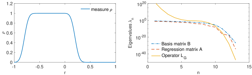
Figure 1: The exploration measure and the eigenvalues of the basis matrix $B$, regression matrix $A_{D}$ and operator ${\mathcal{L}_{\overline{G}}}$ (computed via the generalized eigenvalue problem of $(A_{D},B)$).

The exploration measure (defined in (2.9)) of this dataset has a density

$$\rho(r)=\frac{1}{ZN}\sum_{k=1}^{N}\int_{[0,1]\cap[r,r+1]}\left|u^{k}(y)\right|dy,\quad r\in[-1,1],$$

with $Z$ being the normalizing constant. We set the $\mathcal{H}=\mathrm{span}\{\phi_{i}\}_{i=1}^{l}$, where $\{\phi_{i}\}_{i=1}^{l}$ are B-spline basis functions (i.e., piecewise polynomials) with degree 3 and with knots from a uniform partition of $[-1,1]$. We approximate ${\overline{A}}$ and ${\overline{b}}$ using the Riemann sum integration,

$${\overline{A}}_{D}(i,i^{\prime}) =\frac{1}{N}\sum_{k=1}^{N}\sum_{j=1}^{J}\widehat{R}_{\phi_{i}}[u^{k}](y_{j})\widehat{R}_{\phi_{i^{\prime}}}[u^{k}](y_{j})\triangle y,$$

$${\overline{b}}(i) =\frac{1}{N}\sum_{1\leq k\leq N}\sum_{l=1}^{L}\widehat{R}_{\phi_{i}}[u^{k}](x_{l})f^{k}(y_{l})\triangle y,$$

where we approximate $R_{\psi}[u^{k}]$ via Riemann integration $\widehat{R}_{\psi}[u^{k}](y)=\sum_{j=1}^{J}\psi(y-x_{j})u^{k}(x_{j})\triangle x$. Additionally, to illustrate the effects of discretization error, we also compute ${\overline{A}}$ in (5.3) using the continuous $u^{k}$’s and quadrature integrations, and denote the matrix by ${\overline{A}}_{C}$.

Figure 1 shows the exploration measure and the eigenvalues of the basis matrix $B$, $A_{D}$ and ${\mathcal{L}_{\overline{G}}}$ (which are the generalized eigenvalues of $(A_{D},B)$). Note that the support $\mathcal{S}$ is a proper subset of $[-1,1]$, leading to a near singular $B$. In particular, the inverse problem is severely ill-posed in $L^{2}(\rho)$ since ${\mathcal{L}_{\overline{G}}}$ has multiple almost-zero eigenvalues.

We consider four types of errors (in addition to the observation noise) in ${\overline{b}}$ that often happen in practice.

1. Discretization Error. We assume that $f^{k}$ in (5.8) has no model error.

2. Partial Observation. We assume that $f^{k}$ misses data in the first quarter of the interval, i.e. $f^{k}_{l}=0$ for $l=0,\dots,L/4$. Also, assume that there is no model error.

3. Model Error. Assume there are model error.

4. Wrong Noise Assumption. Assume that $\eta_{l}^{k}$ is actually uniformly distributed on the interval $[-\frac{\sqrt{3}\sigma_{\eta}}{\sqrt{\triangle y}},\frac{\sqrt{3}\sigma_{\eta}}{\sqrt{\triangle y}}]$ to introduce an error caused by a wrong noise assumption. Notice that we add a $\sqrt{3}$ to keep the variance at the same level as the Gaussian prior.

For each of the four cases, we compute the posterior means in Table 2 with the optimal hyper-parameter $\lambda_{*}$ selected by the L-curve method, and report the $L^{2}(\rho)$ error of the function estimators. Additionally, for each of them, we consider different levels of observation noise $\sigma_{\eta}$ in $10^{-1}\sim 10^{-5}$, so as to demonstrate the small noise limit of the posterior mean.

We access the performance of the fixed prior and the data-adaptive prior in Table 2 through the accuracy of their posterior means. We report the interquartile range (IQR, the $75^{th}$, $50^{th}$ and $25^{th}$ percentiles) of the $L^{2}(\rho)$ errors of their posterior means in $200$ independent simulations in which $\phi_{true}$ are randomly sampled.

Two scenarios are considered: $\phi_{true}$ is either inside or outside of the FSOI. To draw samples of $\phi_{true}$ outside of the FSOI, we sample the coefficient $c^{*}$ of $\phi_{true}=\sum_{j=1}^{l}c_{j}^{*}\phi_{j}$ from the fixed prior $\mathcal{N}(0,I_{l})$. Thus, the fixed prior is the true prior. To draw samples of $\phi_{true}$ inside the FSOI, we sample $\phi_{true}=\sum_{j=0}^{l}c_{j}^{*}\psi_{j}$ with $c_{*}$ from $\mathcal{N}(0,I_{3})$, where $\{\psi_{j}=\sum_{i=1}^{l}v_{i,j}\phi_{j}\}$ with $v_{\cdot,j}$ being the $j$-th eigenvector of ${\overline{A}}_{D}$. That is, $\phi_{true}$ is sampled in the low-frequency eigenspace of ${\overline{A}}_{D}$.

Note that the exploration measure, the matrices ${\overline{A}}_{D}$, ${\overline{A}}_{C}$ and $B$ are the same in all these simulations, because they are determined by the data $\{u^{k}\}$ and the basis functions. Thus, we only need to compute ${\overline{b}}$ for each simulation.

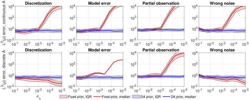
Figure 2: Interquartile range (IQR, the $75^{th}$, $50^{th}$ and $25^{th}$ percentiles) of the $L^{2}(\rho)$ errors of the posterior means. They are computed in $200$ independent simulations with $\phi_{true}$ sampled from the fixed prior (hence outside of the FSOI), in the presence of four types of errors: discretization, model error, partial observation, and wrong noise assumption. Top row: the regression matrix ${\overline{A}}$ is computed from continuous $\{u^{k}\}$; Bottom row: ${\overline{A}}$ is computed from discrete data. The fixed prior leads to diverging posterior means in 6 out of the 8 cases, while the data-adaptive (DA) prior leads to stable posterior means, as the observation noise’s standard deviation $\sigma_{\eta}$ decreases.

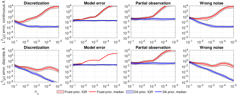
Figure 3: IQR of the $L^{2}(\rho)$ errors of the posterior means in $200$ independent simulations with $\phi_{true}$ sampled inside of the FSOI.

Figure 2 shows the IQR of these simulations in the scenario that the true kernels are outside of the FSOI. The fixed prior leads to diverging posterior means in 6 out of the 8 cases, while the DA-prior has stable posterior means in all cases. The fixed prior has diverging posterior mean when using the continuously integrated regression matrix ${\overline{A}}_{C}$, because the discrepancy between ${\overline{b}}$ and ${\overline{A}}_{C}$ leads to a perturbation outside the FSOI, satisfying Assumption 3.1 (A3). Similarly, either the model error or partial observation error in ${\overline{b}}$ causes a perturbation outside the FSOI of ${\overline{A}}_{D}$, making the fixed prior’s posterior mean diverge. On the other hand, the discretely computed ${\overline{A}}_{D}$ matches ${\overline{b}}$ in the sense that ${\overline{b}}\in{\rm Range}({\overline{A}}_{D})$ as proved in Proposition 5.7, so the fixed prior has a stable posterior mean in cases of discretization and wrong noise assumption. In all these cases, the error of the posterior mean of the DA-prior does not decay as $\sigma_{\eta}\to 0$, because the error is dominated by the part outside of the FSOI that cannot be recovered from data.

Figure 3 shows the IQR of these simulations with the true kernels sampled inside of the FSOI. The DA prior leads to posterior means that are not only stable but also converge to small noise limits, whereas the fixed prior leads to diverging posterior means as in Figure 2. The convergence of the posterior means of the DA prior can be clearly seen in the cases of “Discretization” and “Wrong noise” with both continuously and discretely computed regression matrix. Meanwhile, the flat lines of the DA prior in the cases of “Model error” or “Partial observations” are due to the error inside the FSOI caused by either the model error or partial observation error in ${\overline{b}}$, as shown in the proof of Theorem 4.2.

Additionally, we show in Figure 4 and Figure 5 the estimated posterior (in terms of its mean, the $75^{th}$ and $25^{th}$ percentiles) in a typical simulation, when $\phi_{true}$ is outside and inside the FSOI, respectively. Here the percentiles are computed by drawing samples from the posterior. A more accurate posterior would have a more accurate mean and a narrower shaded region between the percentiles so as to have a smaller uncertainty. In all cases, the DA prior leads to more accurate posterior mean (MAP) than the fixed prior. When the observation noise has $\sigma_{\eta}=0.1$, the DA prior leads to a posterior with a larger shaded region between the percentiles than the fixed prior, but when $\sigma_{\eta}=0.001$, the DA prior’s shaded region is much smaller than those of the fixed prior.

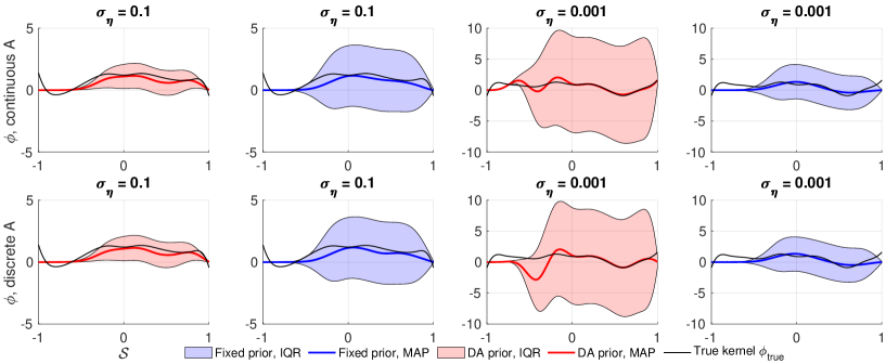
Figure 4: The posterior (its mean, the $75^{th}$ and $25^{th}$ percentiles) when $\phi_{true}\notin$ FSOI.

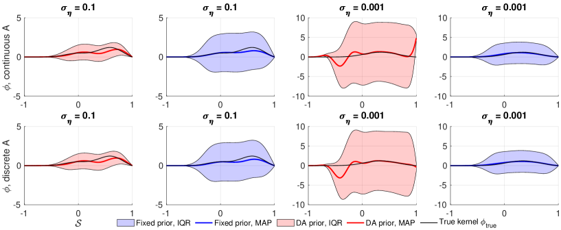
Figure 5: The posterior (its mean, the $75^{th}$ and $25^{th}$ percentiles) when $\phi_{true}\in$ FSOI.

In summary, these numerical results confirm that the data-adaptive prior removes the risk in a fixed non-degenerate prior, leading to a robust posterior with a small noise limit.

5.4 Limitations of the data-adaptive prior

As stated in [24]: “every practical method has its advantages and disadvantages”. The major advantage of the data-adaptive prior is to avoid the posterior being contaminated by the errors outside of the data-dependent function space of identifiability (FSOI), which is the eigenspace with positive eigenvalues of the operator ${\mathcal{L}_{\overline{G}}}$ in the inverse problem. The data-adaptive prior overcomes the ill-posedness caused by a singular operator ${\mathcal{L}_{\overline{G}}}$. Its advantage vanishes when the operator ${\mathcal{L}_{\overline{G}}}$ is well-conditioned, i.e., the inverse problem is well-posed in $L^{2}(\rho)$.

The data-adaptive prior has two disadvantages. First, it relies on the selection of the hyper-parameter $\lambda_{*}$. The L-curve method is the state-of-the-art method and works well in our numerical tests, yet it has limitations in dealing with smoothness and asymptotic consistency [24]. An improper hyper-parameter can lead to a posterior with an inaccurate mean and unreliable covariance. Second, the premise of the data-adaptive prior is that the identifiable part of the true kernel is in the data-adaptive RKHS. But the data-adaptive RKHS can be restrictive when the data is smooth, leading to an overly-smoothed estimator if the true kernel is non-smooth. It remains open to select the covariance operator of the prior in the form of ${\mathcal{L}_{\overline{G}}}^{s}$ with $s\geq 0$ to detect the smoothness of the true kernel. We leave this as potential future work.

6 Conclusion

The inverse problem of learning kernels in operators can be severely ill-posed with a singular inversion operator. The Bayesian approach overcomes the ill-posedness by a non-degenerate prior. However, we show that such a fixed non-degenerate prior leads to a divergent posterior mean when the observation noise becomes small, if the data induces a perturbation in the eigenspace of zero eigenvalues of the inversion operator.

We solve the issue by a data-adaptive prior. It leads to a stable posterior whose mean always has a small noise limit, and the small noise limit converges to the identifiable part of the true kernel when the perturbation vanishes. The data-adaptive prior’s covariance is the inversion operator with a hyper-parameter selected adaptive to data by the L-curve method. Also, the data-adaptive prior improves the quality of the posterior over the fixed prior in two aspects: a smaller expected mean square error of the posterior mean, and a smaller trace of the covariance operator (thus reducing the uncertainty). Furthermore, we provide a detailed analysis on the data-adaptive prior in computational practice. We demonstrate the advantage of the data-adaptive prior on Toeplitz matrices and integral operators in the presence of four types of errors. Numerical tests show that while a fixed non-degenerate prior leads to divergent posterior mean in these cases, the data-adaptive prior always attains posterior means with small noise limits.

We have also discussed the limitations of the data-adaptive prior, such as its dependence on the selection of the hyper-parameter and its tendency of over-smoothing. It is of interest to overcome these limitations in future research by adaptively selecting the regularity of the prior covariance through a fractional operator. Among various other directions to be further explored, we mention one that is particularly relevant in the era of big data: to investigate the inverse problem when the data $\{u^{k}\}$ are randomly sampled in the setting of infinite-dimensional statistical models (e.g., [22]). When the operator $R_{\phi}[u]$ is linear in $u$, the examples of Toeplitz matrices and integral operators show that the inverse problem will become less ill-posed when the number of linearly independent data $\{u^{k}\}$ increases. When $R_{\phi}$ is nonlinear in $u$, it remains open to understand how the ill-posedness depends on the data. Another direction would be to consider sampling the posterior exploiting MCMC or sequential Monte Carlo methodologies (e.g.,[46]).

Appendix A Appendix

A.1 Identifiability theory

The main theme in the identifiability theory is to find the function space in which the quadratic loss functional has a unique minimizer.

The next lemma shows that the inversion operator ${\mathcal{L}_{\overline{G}}}$ defined in (2.12) is a trace-class operator. Recall that an operator $\mathcal{Q}$ on a Hilbert space if it satisfies $\sum_{k}\langle{\mathcal{Q}e_{k},e_{k}}\rangle<\infty$ for any complete orthonormal basis $\{e_{k}\}_{k=1}^{\infty}$.

Lemma A.1.

Under Assumption 2.6, the operator ${\mathcal{L}_{\overline{G}}}:L^{2}(\rho)\to L^{2}(\rho)$ defined in (2.12) is a trace-class operator with $Tr({\mathcal{L}_{\overline{G}}})=\int_{\mathcal{S}}{\overline{G}}(r,r)\rho(r)dr$.

Proof.

We have $\rho(r)=\frac{1}{ZN}\sum_{1\leq k\leq N}\int_{\Omega}\left|g[u^{k}](x,r+x)\right|\mu(dx)$ by (2.9). Then,

$$G(r,s)=\frac{1}{N}\sum_{1\leq k\leq N}\int g[u^{k}](x,r+x)g[u^{k}](x,s+x)\mu(dx)\leq C\rho(r)\wedge\rho(s)$$

for and $r,s\in\mathcal{S}$, where $C=Z\max_{1\leq k\leq K}\sup_{x,y\in\Omega}|g[u^{k}](x,y)|$. Thus,

$${\overline{G}}(r,s)=\frac{G(r,s)}{\rho(r)\rho(s)}\leq C\rho(r)^{-1}\wedge\rho(s)^{-1},$$

for each $r,s\in\mathcal{S}$. Meanwhile, since $\Omega$ is bonded, we have $|\mathcal{S}|<\infty$. Hence $\int_{\mathcal{S}}{\overline{G}}(r,r)\rho(r)dr\leq C|\mathcal{S}|<\infty$. Also, note that ${\overline{G}}$ is continuous since $g[u^{k}]$ is continuous. Then, by [31, Theorem 12, p344], the operator ${\mathcal{L}_{\overline{G}}}$ with integral kernel ${\overline{G}}$ has a finite trace $Tr({\mathcal{L}_{\overline{G}}})=\int_{\mathcal{S}}{\overline{G}}(r,r)\rho(r)dr<\infty$. ∎

Theorem 2.7 characterizes the FSOI through the inversion operator ${\mathcal{L}_{\overline{G}}}$.

Proof of Theorem 2.7.

Part $(a)$ follows from the definition of $\phi^{\scriptscriptstyle\mathcal{D}}$ in (2.15). In fact, plugging in $f^{k}=R_{\phi_{true}}[u^{k}]+\xi_{k}+\eta_{k}$ into the right hand side of (2.15), we have, $\forall\psi\in L^{2}(\rho)$,

$$\langle{\phi^{\scriptscriptstyle\mathcal{D}},\psi}\rangle_{L^{2}(\rho)} =\frac{1}{N}\sum_{1\leq k\leq N}\langle{R_{\psi}[u^{k}],R_{\phi_{true}}[u^{k}]}\rangle_{\mathbb{Y}}+\langle{R_{\psi}[u^{k}],\xi_{k}]}\rangle_{\mathbb{Y}}+\langle{R_{\psi}[u^{k}],\eta_{k}]}\rangle_{\mathbb{Y}}$$

$$=\langle{\psi,{\mathcal{L}_{\overline{G}}}\phi_{true}}\rangle_{L^{2}(\rho)}+\langle{\psi,\epsilon^{\xi}}\rangle_{L^{2}(\rho)}+\langle{\psi,\epsilon^{\eta}}\rangle_{L^{2}(\rho)},$$

where the first term in the last equation comes from the definitions of the operator ${\mathcal{L}_{\overline{G}}}$ in (2.12), the second and the third term comes from the Riesz representation. Since each $\eta_{k}$ is a $\mathbb{Y}$-valued white noise, the random variable $\langle{\psi,\epsilon^{\eta}}\rangle_{L^{2}(\rho)}=\frac{1}{N}\sum_{1\leq k\leq N}\langle{R_{\psi}[u^{k}],\eta_{k}]}\rangle_{\mathbb{Y}}$ is Gaussian with mean zero and variance $\sigma_{\eta}^{2}\langle{\psi,{\mathcal{L}_{\overline{G}}}\psi}\rangle_{L^{2}(\rho)}$ for each $\psi\in L^{2}(\rho)$. Thus, $\epsilon^{\eta}$ has a Gaussian distribution $\mathcal{N}(0,\sigma_{\eta}^{2}{\mathcal{L}_{\overline{G}}})$.

Part $(b)$ follows directly from loss functional in (2.14).

For Part $(c)$, first, note that the quadratic loss functional has a unique minimizer in $H$. Meanwhile, note that $H$ is the orthogonal complement of the null space of ${\mathcal{L}_{\overline{G}}}$, and $\mathcal{E}(\phi_{true}+\phi^{0})=\mathcal{E}(\phi_{true})$ for any $\phi^{0}$ such that ${\mathcal{L}_{\overline{G}}}\phi^{0}=0$. Thus, $H$ is the largest such function space, and we conclude that $H$ is the FSOI.

Next, for any $\phi^{\scriptscriptstyle\mathcal{D}}\in{\mathcal{L}_{\overline{G}}}(L^{2}(\rho))$, the estimator $\widehat{\phi}={\mathcal{L}_{\overline{G}}}^{-1}\phi^{\scriptscriptstyle\mathcal{D}}$ is well-defined. By Part $(b)$, this estimator is the unique zero of the loss functional’s Fréchet derivative in $H$. Hence it is the unique minimizer of $\mathcal{E}(\phi)$ in $H$. In particular, when the data is noiseless and with no model error, and it is generated from $\phi_{true}$, i.e. $R_{\phi_{true}}[u^{k}]=f^{k}$, we have $\phi^{\scriptscriptstyle\mathcal{D}}={\mathcal{L}_{\overline{G}}}\phi_{true}$ from Part $(a)$. Hence $\widehat{\phi}={\mathcal{L}_{\overline{G}}}^{-1}\phi^{\scriptscriptstyle\mathcal{D}}=\phi_{true}$. That is, $\phi_{true}\in H$ is the unique minimizer of the loss functional $\mathcal{E}$. ∎

The proof of Proposition 5.6 is an extension of Theorem 4.1 of [36].

Proof of Proposition 5.6.

Let $\psi_{k}=\sum_{j=1}^{l}V_{jk}\phi_{j}$ with $V^{\top}BV=I$. Then, $\psi_{k}$ is an eigenfunction of ${\mathcal{L}_{\overline{G}}}$ with eigenvalue $\lambda_{k}$ if and only if for each $i$,

$$\langle{\phi_{i},\lambda_{k}\psi_{k}}\rangle_{L^{2}(\rho)}=\langle{\phi_{i},{\mathcal{L}_{\overline{G}}}\psi_{k}}\rangle_{L^{2}(\rho)}=\sum_{1\leq j\leq l}\langle{\phi_{i},{\mathcal{L}_{\overline{G}}}\phi_{j}}\rangle_{L^{2}(\rho)}V_{jk}=\sum_{1\leq j\leq l}{\overline{A}}(i,j)V_{jk},\vspace{-2mm}$$

where the last equality follows from the definition of ${\overline{A}}$. Meanwhile, by the definition of $B$ we have $\langle{\phi_{i},\lambda_{k}\psi_{k}}\rangle_{L^{2}(\rho)}=\sum_{j=1}^{l}B(i,j)V_{jk}\lambda_{k}$ for each $i$. Then, Equation (5.7) follows.

Next, to compute $\langle{\phi,{\mathcal{L}_{\overline{G}}}^{-1}\phi}\rangle_{L^{2}(\rho)}$, we denote $\Psi=(\psi_{1},\ldots,\psi_{l})^{\top}$ and $\Phi=(\phi_{1},\ldots,\phi_{l})^{\top}$. Then, we can write

$$\Psi=V^{\top}\Phi\qquad\phi=\sum_{1\leq i\leq l}c_{i}\phi_{i}=c^{\top}\Phi=c^{\top}V^{-\top}\Psi.$$

Hence, we can obtain $B_{rkhs}=(V\Lambda V^{\top})^{-1}$ in $\langle{\phi,{\mathcal{L}_{\overline{G}}}^{-1}\phi}\rangle_{L^{2}(\rho)}=c^{\top}B_{rkhs}c$ via:

$$\langle{\phi,{\mathcal{L}_{\overline{G}}}^{-1}\phi}\rangle_{L^{2}(\rho)} =\langle{c^{\top}\Phi,{\mathcal{L}_{\overline{G}}}^{-1}c^{\top}\Phi}\rangle_{L^{2}(\rho)}$$

$$=\langle{c^{\top}V^{-\top}\Psi,{\mathcal{L}_{\overline{G}}}^{-1}c^{\top}V^{-\top}\Psi}\rangle_{L^{2}(\rho)}$$

$$=c^{\top}V^{-\top}\langle{\Psi,{\mathcal{L}_{\overline{G}}}^{-1}\Psi}\rangle_{L^{2}(\rho)}V^{-1}c$$ (A.1)

$$=c^{\top}V^{-\top}\Lambda^{-1}V^{-1}c,$$

where the last equality follows from $\langle{\Psi,{\mathcal{L}_{\overline{G}}}^{-1}\Psi}\rangle_{L^{2}(\rho)}=\Lambda^{-1}$.

Additionally, to prove $B_{rkhs}=B{\overline{A}}^{-1}B$, we use the generalized eigenvalue problem. Since $V^{\top}BV=I$, we have $V^{-1}=V^{\top}B$. Meanwhile, ${\overline{A}}V=BV\Lambda$ implied that $B^{-1}{\overline{A}}=V\Lambda V^{-1}$. Thus, $B^{-1}{\overline{A}}B^{-1}=V\Lambda V^{-1}=V\Lambda V^{\top}$, which is $B_{rkhs}^{-1}$. ∎

A.2 Gaussian measures on a Hilbert space

A Gaussian measure on a Hilbert space is defined by its mean and covariance operator (see [11, Chapter 1-2] and [12]). Let $H$ be a Hilbert space with inner product $\langle{\cdot,\cdot}\rangle$, and let $\mathcal{B}(H)$ denote its Borel algebra. Let $\mathcal{Q}$ be a symmetric nonnegative trace class operator on $H$, that is $\langle{\mathcal{Q}x,y}\rangle=\langle{x,\mathcal{Q}y}\rangle$ and $\langle{\mathcal{Q}x,x}\rangle\geq 0$ for any $x,y\in H$, and $\sum_{k}\langle{\mathcal{Q}e_{k},e_{k}}\rangle<\infty$ for any complete orthonormal basis $\{e_{k}\}_{k=1}^{\infty}$. Additionally, denote $\{\lambda_{k},e_{k}\}_{k=1}^{\infty}$ the eigenvalues (in descending order) and eigenfucntions of $\mathcal{Q}$.

A measure on $H$ with mean $a$ and covariance operator $\mathcal{Q}$ is a Gaussian measure $\pi=\mathcal{N}(a,\mathcal{Q})$ iff its Fourier transform $\widehat{\pi}(h)=\int_{H}e^{i\langle{x,h}\rangle}\pi(dx)$ is $e^{i\langle{a,h}\rangle-\frac{1}{2}\langle{\mathcal{Q}h,h}\rangle}$ for any $h\in H$. The measure is non-degenerate if $\mathrm{Ker}\mathcal{Q}=\{0\}$, i.e., $\lambda_{k}>0$ for all $k$. It is a product measure $\pi=\prod_{k=1}^{\infty}\mathcal{N}(a_{k},\lambda_{k})$, where $a_{k}=\langle{a,e_{k}}\rangle\in\mathbb{R}$ for each $k$.

The next lemma specifies the covariance of the coefficient of a Hilbert space valued Gaussian random variable. The coefficient can be on either the full or partial basis.

Lemma A.2 (Operator to coefficients).

Let $\mathcal{N}(0,\mathcal{Q})$ be a Gaussian measure on $H$ and let the hypothesis space $\mathcal{H}=\mathrm{span}\{\phi_{i}\}_{i=1}^{l}\subset H$ with $l\leq\infty$ have basis such that the matrix $B=\langle{\phi_{i},\phi_{j}}\rangle_{1\leq i,j\leq l}$ is strictly positive definite. Then, the coefficient $c\in\mathbb{R}^{l}$ of $\phi=\sum_{i=1}^{l}c_{i}\phi_{i}$ has a Gaussian measure $\mathcal{N}(0,B^{-1}AB^{-1})$, where the matrix $A(i,j)=\langle{\phi_{i},\mathcal{Q}\phi_{j}}\rangle$.

Proof.

By definition, for any $h\in\mathcal{H}$, the random variable $\langle{\phi,h}\rangle$ has distribution $\mathcal{N}(0,\langle{h,\mathcal{Q}h}\rangle)$. Thus, we have $\langle{\phi,\phi_{k}}\rangle\sim\mathcal{N}(0,\langle{\phi_{k},\mathcal{Q}\phi_{k}}\rangle)$ for each $k$. Similarly, we have that
$\mathbb{E}[\langle{\phi,\phi_{k}+\phi_{l}}\rangle^{2}]=\langle{\phi_{k}+\phi_{l},\mathcal{Q}(\phi_{k}+\phi_{l})}\rangle$. Then, we have

$$\mathbb{E}[\langle{\phi,\phi_{k}}\rangle\langle{\phi,\phi_{l}}\rangle]=\frac{1}{2}\left(\mathbb{E}[\langle{\phi,\phi_{k}+\phi_{l}}\rangle^{2}]-\mathbb{E}[\langle{\phi,\phi_{k}}\rangle^{2}]-\mathbb{E}[\langle{\phi,\phi_{k}}\rangle^{2}]\right)=\langle{\phi_{k},\mathcal{Q}\phi_{l}}\rangle.$$

Hence, the random vector $X=(\langle{\phi,\phi_{1}}\rangle,\ldots,\langle{\phi,\phi_{l}}\rangle)^{\top}$ is Gaussian $\mathcal{N}(0,A)$. Now, noticing that $X=Bc$ and $B=B^{\top}$, we obtain that the distribution of $c=B^{-1}X$ is $\mathcal{N}(0,B^{-1}AB^{-1})$, where the covariance follows from $\mathbb{E}[cc^{\top}]=\mathbb{E}[B^{-1}XX^{\top}B^{-1}]=B^{-1}AB^{-1}$. ∎

On the other hand, the distribution of the coefficient only determines a Gaussian measure on the linear space its basis spans.

Lemma A.3 (Coefficients to operator).

Let $\mathcal{H}=\mathrm{span}\{\phi_{i}\}_{i=1}^{l}$ with $l\leq\infty$ be a Hilbert space with basis such that the matrix $B=\langle{\phi_{i},\phi_{j}}\rangle_{1\leq i,j\leq l}$ is strictly positive definite. Let the coefficient $c\in\mathbb{R}^{l}$ of $\phi=\sum_{i=1}^{l}c_{i}\phi_{i}$ have a Gaussian measure $\mathcal{N}(0,Q)$. Then, the $\mathcal{H}$-valued random variable $\phi$ has a Gaussian distribution $\mathcal{N}(0,\mathcal{Q})$, where the operator $\mathcal{Q}$ is defined by $\langle{\phi_{i},\mathcal{Q}\phi_{j}}\rangle=(BQB)_{i,j}$.

Proof.

Since $\{\phi_{i}\}$ is a complete basis, we only need to determine the distribution of the random vector $X=(\langle{\phi,\phi_{1}}\rangle,\ldots,\langle{\phi,\phi_{l}}\rangle)^{\top}\in\mathbb{R}^{l}$. Note that it satisfies $X=Bc$. Thus, its distribution is Gaussian $\mathcal{N}(0,BQB)$. ∎

Note that $\pi(\mathcal{Q}^{1/2}H)=0$ if $H$ is infinite-dimensional, that is, the Cameron-Martin space $\mathcal{Q}^{1/2}H$ has measure zero.

A.3 Details of numerical examples

Computation for Toeplitz matrix.

Each dataset $\{u^{k}=(u_{0}^{k},u_{1}^{k})\}_{k}$ leads to an exploration measure on $\mathcal{S}=\{-1,0,1\}$:

$$\rho(-1)=\frac{\sum_{k}|u_{1}^{k}|}{2\sum_{k}(|u_{1}^{k}|+|u_{0}^{k}|)},\quad\rho(0)=\frac{1}{2},\quad\rho(1)=\frac{\sum_{k}|u_{0}^{k}|}{2\sum_{k}(|u_{1}^{k}|+|u_{0}^{k}|)}.$$

Since each $u=(u_{0},u_{1})$ leads to a rank-2 regression matrix

$$L_{u}=\begin{bmatrix}u_{1}&u_{0}&0\\ 0&u_{1}&u_{0}\end{bmatrix},\quad L_{u}^{\top}L_{u}=\begin{bmatrix}u_{1}^{2}&u_{1}u_{0}&0\\ u_{1}u_{0}&u_{1}^{2}+u_{0}^{2}&u_{1}u_{0}\\ 0&u_{1}u_{0}&u_{0}^{2}\end{bmatrix},$$

the regression matrices ${\overline{A}}=\sum_{k}L_{u^{k}}^{\top}L_{u^{k}}$ of the three datasets are

$${\overline{A}}_{(1)}=\begin{bmatrix}0&0&0\\ 0&1&0\\ 0&0&1\end{bmatrix},\quad{\overline{A}}_{(2)}=\frac{1}{2}\sum_{k=1}^{2}L_{u^{k}}^{\top}L_{u^{k}}=\frac{1}{2}\begin{bmatrix}1&0&0\\ 0&2&0\\ 0&0&1\end{bmatrix},\quad{\overline{A}}_{(3)}=\begin{bmatrix}1&1&0\\ 1&2&1\\ 0&1&1\end{bmatrix}.$$ (A.2)

Additionally, with $B=\mathrm{Diag}(\rho)$, the prior covariances $\lambda_{*}Q_{0}^{\scriptscriptstyle\mathcal{D}}=B^{-1}{\overline{A}}B^{-1}$ are

$$Q^{\scriptscriptstyle\mathcal{D}}_{0,(1)}=\begin{bmatrix}0&0&0\\ 0&4&0\\ 0&0&4\end{bmatrix},\quad Q^{\scriptscriptstyle\mathcal{D}}_{0,(2)}=\begin{bmatrix}8&0&0\\ 0&4&0\\ 0&0&8\end{bmatrix},\quad Q^{\scriptscriptstyle\mathcal{D}}_{0,(3)}=\begin{bmatrix}16&8&0\\ 8&8&8\\ 0&8&16\end{bmatrix}.$$ (A.3)

We analyze the well-posedness of the inverse problem in terms of the operator ${\mathcal{L}_{\overline{G}}}$, whose eigenvalues are solved via the generalized eigenvalue problem (see Proposition 5.6). For the data set $\{u^{1}\}$, the exploration measure $\rho$ is degenerate with $\rho(-1)=0$, thus, we have no information from data to identify $\phi(-1)$. As a result, $L^{2}(\rho)=\mathrm{span}\{\phi_{2},\phi_{3}\}$ is a proper subspace of $\mathbb{R}^{3}$. The regression matrix ${\overline{A}}_{(1)}$ and the covariance matrix $Q^{\scriptscriptstyle\mathcal{D}}_{0,(1)}$ are effectively the identity matrix $I_{2}$ and $4I_{2}$. The operator ${\mathcal{L}_{\overline{G}}}$ has eigenvalues $\{1,1\}$, and the FSOI is $L^{2}(\rho)$. Thus, the inverse problem is well-posed in $L^{2}(\rho)$. For the dataset $\{u^{1},u^{2}\}$, the inverse problem is also well-posed in $L^{2}(\rho)$ because the operator ${\mathcal{L}_{\overline{G}}}$ has eigenvalues $\{2,2,2\}$, and the FSOI is $L^{2}(\rho)$. Note that the data-adaptive prior $Q^{\scriptscriptstyle\mathcal{D}}_{0,(2)}$ assigns weights to the entries of the coefficient according to the exploration measure. For the data set $\{u^{3}\}$, the inverse problem is ill-defined in $L^{2}(\rho)$, but it is well-posed in the FSOI, which is a proper subset of $L^{2}(\rho)$. Here the FSOI is the linear span of $\{\psi_{1},\psi_{2}\}$, which are the eigenvectors of ${\mathcal{L}_{\overline{G}}}$ with positive eigenvalues. Following (5.7), these eigenvectors $\{\psi_{i}\}$ are solved from the generalized eigenvalue problem ${\overline{A}}_{(3)}\psi=\lambda\mathrm{Diag}(\rho)\psi$ and they are orthonormal in $L^{2}(\rho)$. The eigenvalues are $\{8,4,0\}$ and the corresponding eigenvectors are $\psi_{1}=(1,1,1)^{\top}$, $\psi_{2}=(-\sqrt{2},0,\sqrt{2})^{\top},$ and $\psi_{3}=(1,-1,1)^{\top}$.

The hyper-parameter selected by the L-curve method.

We select the hyper-parameter $\lambda_{*}$ in the data-adaptive prior by the L-curve method. Figure 6 shows a typical L-curve, where $\mathcal{R}(\lambda)=\left\|\phi_{\lambda}\right\|_{H_{G}}$ and $\mathcal{E}$ represents the square root of the loss $\mathcal{E}(\phi_{\lambda})$. The L-curve method selects the parameter that attains the maximal curvature at the corner of the $L$ shaped curve.

Figures 7–8 present the $\lambda_{*}$ in the simulations in Figures 2– 3, respectively. Those hyper-parameters are mostly similar, and the majority of them are at the scale of $10^{-4}$. They show that the optimal hyper-parameter depends on the spectrum of ${\mathcal{L}_{\overline{G}}}$, the four types of the errors in ${\overline{b}}$, the strength of the noise, and the smoothness of the true kernel. In general, a large variation of $\lambda_{*}$ suggests a difficulty in selecting an optimal hyper-parameter by the method. Additionally, the error in the numerical computation of matrix inversion or the solution of the linear systems can affect the result when $\lambda_{*}$ is small. Thus, it is complicated to analyze the optimal hyper-parameter.

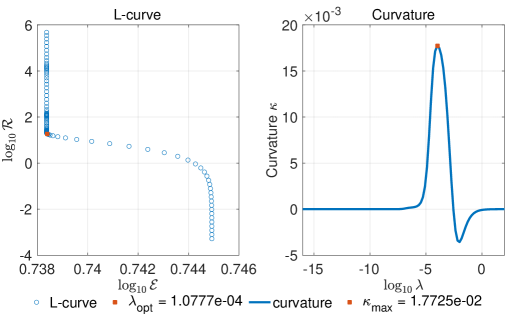
Figure 6: The L-curve for the selection of the hyper-parameter $\lambda_{*}$.

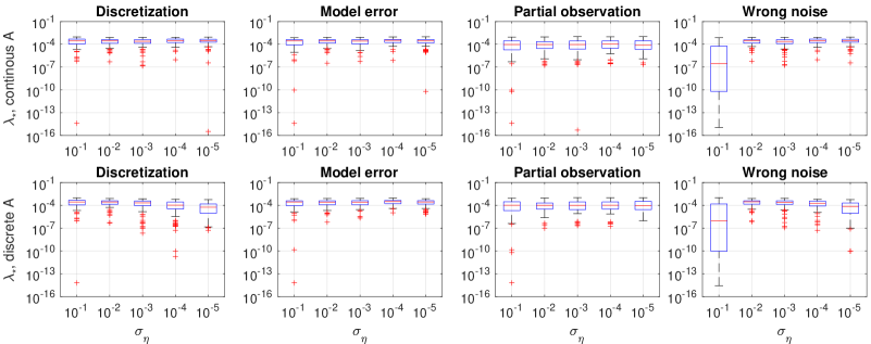
Figure 7: The hyper-parameter $\lambda_{*}$ in the 200 simulations in Figure 2.

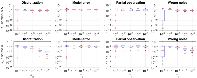
Figure 8: The hyper-parameter $\lambda_{*}$ in the 200 simulations in Figure 3.

References

- [1] A. Agliari and C. C. Parisetti. A-g reference informative prior: A note on zellner’s prior. Journal of the Royal Statistical Society. Series D (The Statistician), 37(3):271–275, 1988.
- [2] A. Alexanderian, P. J. Gloor, and O. Ghattas. On bayesian a-and d-optimal experimental designs in infinite dimensions. Bayesian Analysis, 11(3):671–695, 2016.
- [3] F. Bauer, S. Pereverzev, and L. Rosasco. On regularization algorithms in learning theory. Journal of complexity, 23(1):52–72, 2007.
- [4] M. J. Bayarri, J. O. Berger, A. Forte, and G. García-Donato. Criteria for bayesian model choice with application to variable selection. The Annals of Statistics, 40(3), Jun 2012.
- [5] M. Belkin, S. Ma, and S. Mandal. To understand deep learning we need to understand kernel learning. In International Conference on Machine Learning, pages 541–549. PMLR, 2018.
- [6] C. Bucur and E. Valdinoci. Nonlocal Diffusion and Applications, volume 20 of Lecture Notes of the Unione Matematica Italiana. Springer International Publishing, Cham, 2016.
- [7] J. A. Carrillo, K. Craig, and Y. Yao. Aggregation-diffusion equations: dynamics, asymptotics, and singular limits. In Active Particles, Volume 2, pages 65–108. Springer, 2019.
- [8] K. Chaloner and I. Verdinelli. Bayesian experimental design: A review. Statistical Science, pages 273–304, 1995.
- [9] F. Cucker and D. X. Zhou. Learning theory: an approximation theory viewpoint, volume 24. Cambridge University Press, 2007.
- [10] T. Cui and X. T. Tong. A unified performance analysis of likelihood-informed subspace methods. Bernoulli, 28(4):2788–2815, 2022.
- [11] G. Da Prato. An introduction to infinite-dimensional analysis. Springer Science & Business Media, 2006.
- [12] G. Da Prato and J. Zabczyk. Stochastic equations in infinite dimensions. Cambridge university press, 2014.
- [13] M. Darcy, B. Hamzi, J. Susiluoto, A. Braverman, and H. Owhadi. Learning dynamical systems from data: a simple cross-validation perspective, part ii: nonparametric kernel flows. 2021.
- [14] M. Dashti and A. M. Stuart. The bayesian approach to inverse problems. In Handbook of uncertainty quantification, pages 311–428. Springer, 2017.
- [15] M. V. de Hoop, D. Z. Huang, , E. Quin, and A. M. Stuart. The cost-accuracy trade-off in operator learning with neural networks. arXiv preprint arXiv:2203.13181, 2022.
- [16] M. V. de Hoop, N. B. Kovachki, , N. H. Nelsen, and A. M. Stuart. Convergence rates for learning linear operators from noisy data. SIAM/ASA Journal on Uncertainty Quantification, 2022.
- [17] M. D’Elia, Q. Du, C. Glusa, M. Gunzburger, X. Tian, and Z. Zhou. Numerical methods for nonlocal and fractional models. Acta Numerica, 29:1–124, 2020.
- [18] L. Della Maestra and M. Hoffmann. Nonparametric estimation for interacting particle systems : McKean-Vlasov models. ArXiv201103762 Math Stat, 2021.
- [19] Q. Du, M. Gunzburger, R. B. Lehoucq, and K. Zhou. Analysis and Approximation of Nonlocal Diffusion Problems with Volume Constraints. SIAM Rev., 54(4):667–696, 2012.
- [20] J. Feng, Y. Ren, and S. Tang. Data-driven discovery of interacting particle systems using gaussian processes. arXiv preprint arXiv:2106.02735, 2021.
- [21] S. Gazzola, P. C. Hansen, and J. G. Nagy. Ir tools: a matlab package of iterative regularization methods and large-scale test problems. Numerical Algorithms, 81(3):773–811, 2019.
- [22] E. Giné and R. Nickl. Mathematical foundations of infinite-dimensional statistical models, volume 40. Cambridge University Press, 2015.
- [23] P. C. Hansen. REGULARIZATION TOOLS: A Matlab package for analysis and solution of discrete ill-posed problems. Numer Algor, 6(1):1–35, 1994.
- [24] P. C. Hansen. The L-curve and its use in the numerical treatment of inverse problems. In in Computational Inverse Problems in Electrocardiology, ed. P. Johnston, Advances in Computational Bioengineering, pages 119–142. WIT Press, 2000.
- [25] Y. He, S. H. Kang, W. Liao, H. Liu, and Y. Liu. Numerical identification of nonlocal potential in aggregation. arXiv preprint arXiv:2207.03358, 2022.
- [26] T. Hofmann, B. Schölkopf, and A. J. Smola. Kernel methods in machine learning. Ann. Statist., 36(3):1171–1220, 06 2008.
- [27] J. Kaipio and E. Somersalo. Statistical and Computational Inverse Problems. Springer, 2005.
- [28] N. B. Kovachki, Z. Li, K. Azizzadenesheli, B. Liu, K. Bhattacharya, A. M. Stuart, and A. Anandkumar. Neural operator: Learning maps between function spaces. arXiv preprint arXiv:2108.08481, 2021.
- [29] Q. Lang and F. Lu. Identifiability of interaction kernels in mean-field equations of interacting particles. arXiv preprint arXiv:2106.05565, 2021.
- [30] Q. Lang and F. Lu. Learning interaction kernels in mean-field equations of first-order systems of interacting particles. SIAM Journal on Scientific Computing, 44(1):A260–A285, 2022.
- [31] P. D. Lax. Functional Analysis. John Wiley & Sons Inc., New York, 2002.
- [32] M. S. Lehtinen, L. Paivarinta, and E. Somersalo. Linear inverse problems for generalised random variables. Inverse Problems, 5(4):599–612, 1989.
- [33] Z. Li, F. Lu, M. Maggioni, S. Tang, and C. Zhang. On the identifiability of interaction functions in systems of interacting particles. Stochastic Processes and their Applications, 132:135–163, 2021.
- [34] Z. Li, N. B. Kovachki, , K. Azizzadenesheli, B. Liu, K. Bhattacharya, A. M. Stuart, and A. Anandkumar. Fourier neural operator for parametric partial differential equations. International Conference on Learning Representations, 2020.
- [35] F. Lu, Q. An, and Y. Yu. Nonparametric learning of kernels in nonlocal operators. arXiv preprint arXiv2205.11006, 2022.
- [36] F. Lu, Q. Lang, and Q. An. Data adaptive RKHS Tikhonov regularization for learning kernels in operators. Proceedings of Mathematical and Scientific Machine Learning, PMLR 190:158-172, 2022.
- [37] F. Lu, M. Maggioni, and S. Tang. Learning interaction kernels in heterogeneous systems of agents from multiple trajectories. Journal of Machine Learning Research, 22(32):1–67, 2021.
- [38] F. Lu, M. Maggioni, and S. Tang. Learning interaction kernels in stochastic systems of interacting particles from multiple trajectories. Foundations of Computational Mathematics, pages 1–55, 2021.
- [39] F. Lu, M. Zhong, S. Tang, and M. Maggioni. Nonparametric inference of interaction laws in systems of agents from trajectory data. Proc. Natl. Acad. Sci. USA, 116(29):14424–14433, 2019.
- [40] L. Lu, P. Jin, and G. E. Karniadakis. Deeponet: Learning nonlinear operators for identifying differential equations based on the universal approximation theorem of operators. arXiv preprint arXiv:1910.03193, 2021.
- [41] L. Lu, P. Jin, G. Pang, Z. Zhang, and G. E. Karniadakis. Learning nonlinear operators via deeponet based on the universal approximation theorem of operators. Nature Machine Intelligence, 3(3):218–229, 2021.
- [42] C. Mavridis, A. Tirumalai, and J. Baras. Learning swarm interaction dynamics from density evolution. arXiv preprint arXiv:2112.02675, 2021.
- [43] D. A. Messenger and D. M. Bortz. Learning mean-field equations from particle data using WSINDy. Physica D: Nonlinear Phenomena, 439:133406, 2022.
- [44] S. Motsch and E. Tadmor. Heterophilious Dynamics Enhances Consensus. SIAM Rev, 56(4):577 – 621, 2014.
- [45] H. Owhadi and G. R. Yoo. Kernel flows: From learning kernels from data into the abyss. Journal of Computational Physics, 389:22–47, 2019.
- [46] C. Robert and G. Casella, editors. Monte Carlo Statistical Methods. Springer, 1999.
- [47] L. I. Rudin, S. Osher, and E. Fatemi. Nonlinear total variation based noise removal algorithms. Physica D: nonlinear phenomena, 60(1-4):259–268, 1992.
- [48] L. F. Shampine. Vectorized adaptive quadrature in matlab. Journal of Computational and Applied Mathematics, 211(2):131–140, 2008.
- [49] A. Spantini, A. Solonen, T. Cui, J. Martin, L. Tenorio, and Y. Marzouk. Optimal low-rank approximations of bayesian linear inverse problems. SIAM Journal on Scientific Computing, 37(6):A2451–A2487, 2015.
- [50] B. K. Sriperumbudur, K. Fukumizu, and G. R. Lanckriet. Universality, characteristic kernels and RKHS embedding of measures. Journal of Machine Learning Research, 12(70):2389–2410, 2011.
- [51] A. M. Stuart. Inverse problems: a Bayesian perspective. Acta Numer., 19:451–559, 2010.
- [52] R. Tibshirani. Regression Shrinkage and Selection Via the Lasso. Journal of the Royal Statistical Society: Series B (Methodological), 58(1):267–288, 1996.
- [53] A. N. Tihonov. Solution of incorrectly formulated problems and the regularization method. Soviet Math., 4:1035–1038, 1963.
- [54] R. Yao, X. Chen, and Y. Yang. Mean-field nonparametric estimation of interacting particle systems. arXiv preprint arXiv:2205.07937, 2022.
- [55] H. You, Y. Yu, S. Silling, and M. D’Elia. A data-driven peridynamic continuum model for upscaling molecular dynamics. Computer Methods in Applied Mechanics and Engineering, 389:114400, 2022.
- [56] H. You, Y. Yu, N. Trask, M. Gulian, and M. D’Elia. Data-driven learning of nonlocal physics from high-fidelity synthetic data. Computer Methods in Applied Mechanics and Engineering, 374:113553, 2021.
- [57] M. Yuan and T. T. Cai. A reproducing kernel Hilbert space approach to functional linear regression. The Annals of Statistics, 38(6):3412–3444, 2010.
- [58] A. Zellner and A. Siow. Posterior odds ratios for selected regression hypotheses. Trabajos de Estadistica Y de Investigacion Operativa, 31:585–603, 1980.