Attractors of Hamiltonian nonlinear partial differential equations

Abstract

We survey the theory of attractors of nonlinear Hamiltonian partial differential equations since its appearance in 1990. These are results on global attraction to stationary states, to solitons and to stationary orbits, on adiabatic effective dynamics of solitons and their asymptotic stability. Results of numerical simulations are also given. Based on these results, we propose a new general hypothesis on attractors of $G$-invariant nonlinear Hamiltonian partial differential equations. The obtained results suggest a novel dynamical interpretation of basic quantum phenomena: Bohr’s transitions between quantum stationary states, wave-particle duality, and probabilistic interpretation.

To the memory of Mark Vishik

1 Introduction

Theory of attractors of nonlinear PDEs originated from the seminal paper of Landau [B9] published in 1944, where he suggested the first mathematical interpretation of turbulence as the growth of the dimension of attractors of the Navier–Stokes equations when the Reynolds number increases. Modern development of the theory of attractors for general dissipative systems, i.e., systems with friction (the Navier–Stokes equations, nonlinear parabolic equations, reaction-diffusion equations, wave equations with friction, etc.) originated in the 1975–1985’s in the works of Foias, Hale, Henry, Temam, and others [B5]–[B10]. M.I. Vishik together with his collaborators worked on global attractors of dissipative nonlinear PDEs from 1980 until 2012. These investigations had significantly advanced this theory [B1]–[B4].

A typical result of this theory, in the absence of external excitation, is a global convergence to stationary states: for any finite energy solution to dissipative autonomous equation in a region $\Omega\subset\mathbb{R}^{n}$, there is a convergence

$$\psi(x,t)\to S(x),\qquad t\to+\infty.$$ (1.1)

Here $S(x)$ is a stationary solution, depending on the initial state $\psi(x,0)$. As a rule, the convergence holds in the $L^{2}(\Omega)$-metric. In particular, the relaxation to an equilibrium regime in chemical reactions is due to the energy dissipation.

A development of a similar theory for Hamiltonian PDEs looked unmotivated and even impossible since the convergence (1.1) seemed to contradict the energy conservation and time reversibility admitted by these equations. On the other hand, such a theory of global attractors is indispensable for mathematical foundation of quantum physics, since all fundamental PDEs of quantum theory are Hamiltonian: the Maxwell, Schrödinger, Klein–Gordon, Dirac, Yang–Mills equations, etc. Even the shape of the theory is already suggested by fundamental postulates of quantum physics. In particular, the global attraction of type (1.1) is suggested by Bohr’s postulates of 1913 on transitions between quantum stationary states. Namely, the postulate can be interpreted as the global attraction of all quantum trajectories to an attractor formed by quantum stationary states. Such a global convergence also allows us to give a mathematical interpretation to the L. de Broglie wave particle duality and to the M. Born probabilistic interpretation; for more details, see [E7, A13, A14, A15]. We note that in 1961 W. Heisenberg began developing a nonlinear theory of elementary particles [P5, P6].

Thus, the basic postulates of quantum physics suggest the type of long-time behavior of solutions of the related fundamental dynamical equations: Maxwell–Schrödinger, Maxwell–Dirac, Yang–Mills–Dirac, and other equations and systems. All these coupled equations are nonlinear Hamiltonian systems of partial differential equations, and it seems unlikely that these and other fundamental dynamical equations of quantum physics are exceptional among generic Hamiltonian PDEs. This situation leads to the conjecture that the global convergence to a proper attractor is an inherent feature of general nonlinear Hamiltonian PDEs.

The first results on attractors for the Hamiltonian equations were obtained by Morawetz, Segal, and Strauss in the case when the attractor consists of the single point zero. In this case the attraction is called local energy decay [C1]–[C7].

It was not until 1990 when the case of a nontrivial attractor was considered, when the hypothesis on the global attractors was set forth by one of the authors. Since then, this hypothesis has been developed in collaboration with the international group of researchers: with M. Kunze, H. Spohn, and B. Vainberg and later with V.S. Buslaev, A. Comech, V. Imaykin, E. Kopylova, D. Stuart, and others.

The investigations since 1990 suggest that such long-time behavior of solutions is not merely the peculiarity of the dynamical equations of quantum physics, but rather a characteristic property of generic nonlinear Hamiltonian PDEs; see the surveys [E7, E8, E9]. Below, we sketch these results. All these results were discussed in many talks by the authors at the seminars of M.I. Vishik in the Department of Mechanics and Mathematics of Moscow State University.

This theory differs significantly from the theory of attractors of dissipative systems where the attraction to stationary states is due to an energy dissipation caused by a friction. For Hamiltonian equations the friction and energy dissipation are absent, and the attraction is caused by radiation which irrevocably brings the energy to infinity. It is exactly this radiation that is addressed in the Bohr postulate on transitions between quantum stationary states.

2 Bohr’s postulates: quantum jumps

In 1913, Bohr formulated the following two fundamental postulates of the quantum theory of atoms [A4]:

I. Each electron lives on one of the quantum stationary orbits, and sometimes it jumps from one stationary orbit to another: in the Dirac notation,

$$|E_{n}\rangle\mapsto|E_{n^{\prime}}\rangle.$$ (2.1)

II. On a stationary orbit, the electron does not radiate, while every jump is followed by the radiation of an electromagnetic wave of frequency

$$\omega_{nn^{\prime}}=\frac{E_{n^{\prime}}-E_{n}}{\hbar}=\omega_{n^{\prime}}-\omega_{n},\qquad\omega_{n}:=E_{n}/\hbar.$$ (2.2)

Both these postulates were inspired by stability of atoms, by the Rydberg–Ritz Combination Principle, and by the Einstein theory of the photoeffect.

In 1926, with the discovery of the Schrödinger theory [A25], the question arose about the implementation of the above Bohr axioms in the new theory based on partial differential equations. This and other questions have been frequently addressed in the 1920s and 1930s in heated discussions by N. Bohr, E. Schrödinger, A. Einstein, and others [A5]. However, a satisfactory solution was not achieved, and a rigorous dynamical interpretation of these postulates is still unknown. This lack of theoretical clarity hinders a further progress in the theory (e.g., in superconductivity and in nuclear reactions) and in numerical simulation of many engineering processes (e.g., laser radiation and quantum amplifiers), since a computer can solve dynamical equations, but cannot take into account postulates.

3 Schrödinger’s identification of stationary orbits

Besides the equation for the wave function, the Schrödinger theory contains a highly nontrivial definition of stationary orbits (or quantum stationary states) in the case when the Maxwell external potentials do not depend on time: in this case, the Schrödinger equation reads as

$$i\hbar\dot{\psi}(x,t)=H\psi(t):=\frac{1}{2{\rm m}}\Big{[}-i\hbar\nabla-\displaystyle\frac{e}{c}\mathbf{A}_{\mathrm{ext}}(x)\Big{]}^{2}\psi(x,t)+eA_{\mathrm{ext}}^{0}(x)\psi(x,t),$$ (3.1)

where $m$ and $e$ denote the electron’s mass and charge, $c$ is the speed of light in vacuum, $\mathbf{A}_{\mathrm{ext}}(x)$ is the external magnetic potential, and $A_{\mathrm{ext}}^{0}(x)$ is the external scalar potential. In the unrationalized  Gaussian units, also called the Heaviside–Lorentz units [A12, p. 781], the values of the physical constants (the electron charge and mass, the speed of light in vacuum, the Boltzmann constant, and the Planck constant) are approximately equal to

$$\left.\begin{array}[]{c}e=-4.8\times 10^{-10}{\mathrm{esu}},\qquad{\rm m}=9.1\times 10^{-28}{\mathrm{g}},\quad c=3.0\times 10^{10}{\mathrm{cm/s}}\\ \\ k=1.38\times 10^{-16}{\mathrm{erg/K}},\qquad\,\,\hbar=1.1\times 10^{-27}\mathrm{erg}\cdot\mathrm{s}\end{array}\right|.$$ (3.2)

In Schrödinger’s theory [A25], stationary orbits are identified with finite energy solutions of the form

$$\psi(x,t)=\varphi_{\omega}(x)e^{-i\omega t},\qquad\omega\in\mathbb{R}.$$ (3.3)

Substitution of this Ansatz into the Schrödinger equation (3.3) leads to the famous eigenvalue problem

$$\omega\varphi_{\omega}=H\varphi_{\omega},$$ (3.4)

which determines the corresponding frequencies $\omega$ and amplitudes $\varphi_{\omega}$; the latter are subject to the normalization condition

$$\int|\varphi_{\omega}(x)^{2}|\,dx=1.$$ (3.5)

This condition means that the wave function describes one electron, as discussed below.

Such definition is rather natural, since then $|\psi(x,t)|$ does not depend on time. Most likely, this definition was suggested by the de Broglie wave function for free particles $\psi(x,t)=Ce^{i(kx-\omega t)}$, which factorizes as $Ce^{ikx}e^{-i\omega t}$. Indeed, in the case of bound particles, it is natural to change the spatial factor $Ce^{ikx}$, since the spatial properties have changed and ceased to be homogeneous. On the other hand, the homogeneous time factor $e^{-i\omega t}$ must be preserved, since the external potentials are independent of time. However, these ‘‘algebraic’’ arguments do not withdraw the question of agreement of the Schrödinger definition with the Bohr postulate (2.1)!

Thus, the problem of the mathematical interpretation of the Bohr postulate (2.1) in the Schrödinger theory arises. One of the simplest interpretations of the jumps (2.1), (2.2) is the long-time asymptotics

$$\psi(x,t)\sim\psi_{\pm}(x)e^{-i\omega_{\pm}t},\qquad t\to\pm\infty$$ (3.6)

for each finite energy solution, where $\omega_{-}=\omega_{n}$ and $\omega_{+}=\omega_{n^{\prime}}$. However, for the linear Schrödinger equation (3.1), such asymptotics are obviously wrong due to the superposition principle: for example, such asymptotics can not hold for solutions of the form $\psi(x,t)\equiv\phi_{1}(x)e^{-i\omega_{1}t}+\phi_{2}(x)e^{-i\omega_{2}t}$ with $\omega_{1}\neq\omega_{2}$ and with nonzero $\phi_{1}$ and $\phi_{2}$. It is exactly this contradiction that shows that the linear Schrödinger equation alone cannot serve as the basis for the theory compatible with the Bohr postulates.

Remark 3.1.

The Schrödinger definition (3.3) has been formalized by P. Dirac [A6] and J. von Neumann [A22]: they have identified quantum states with the rays in the Hilbert space, so the entire circular orbit (3.3) corresponds to one quantum state. Our main conjecture is that this formalization is indeed a theorem: namely, we suggest that the asymptotics (3.6) is an inherent property of the nonlinear Maxwell–Schrödinger system (see (4.7)–(4.8) below). This conjecture is confirmed by perturbative arguments below.

4 Coupled Maxwell–Schrödinger equations

As we have seen, the linear Schrödinger equation cannot explain the Bohr postulates. Thus, one should look for a nonlinear theory. Fortunately, we do not need to invent anything artificial since such a theory is well established since 1926: it is the system of the Schrödinger equation coupled to the Maxwell equations which was essentially introduced in the first of Schrödinger’s articles [A25]. The corresponding second-quantized system is the main subject of nonrelativistic Quantum Electrodynamics.

This coupled system arises in the following way. The wave function $\psi(x,t)$ defines the corresponding charge and current densities, which, in turn, generate their own Maxwell field. The corresponding potentials of this own field should be added to the external Maxwell potentials in the Schrödinger equation (3.1). This modification implies the nonlinear interaction between the wave function and the Maxwell field. More precisely, the Schrödinger theory associates to the wave function $\psi(x,t)$ the corresponding charge and current densities

$$\rho(x,t)=e|\psi(x,t)|^{2},\qquad\mathbf{j}(x,t)=\frac{e}{{\rm m}}\mathop{\rm Re}\Big{(}\overline{\psi}(x,t)\Big{[}-i\hbar\nabla-\frac{e}{c}\mathbf{A}_{\mathrm{ext}}(x,t)\Big{]}\psi(x,t)\Big{)}.$$ (4.1)

For any solution of the Schrödinger equation (3.1), these densities satisfy the charge continuity equation

$$\dot{\rho}(x,t)+\mathop{\mathrm{div}}\mathbf{j}(x,t)=0.$$ (4.2)

Note that the normalization condition (3.5) means that the total charge corresponding to the stationary orbit (3.3) is

$$\int\rho(x)\,dx=e,$$ (4.3)

i.e., we have exactly one electron on this orbit. The charge and current densities (4.1) generate the Maxwell field according to the Maxwell equations

$$\begin{cases}\mathop{\mathrm{div}}\mathbf{E}(x,t)=\rho(x,t),\quad&\mathop{\mathrm{curl}}\mathbf{E}(x,t)=-\frac{1}{c}\dot{\mathbf{B}}(x,t),\\[8.61108pt] \mathop{\mathrm{div}}\mathbf{B}(x,t)=0,\quad&\mathop{\mathrm{curl}}\mathbf{B}(x,t)=\frac{1}{c}\big{(}\mathbf{j}(x,t)+\dot{\mathbf{E}}(x,t)\big{)}.\end{cases}$$ (4.4)

The second and third equations imply the Maxwell representations

$$\mathbf{B}(x,t)=\mathop{\mathrm{curl}}\mathbf{A}(x,t),\qquad\mathbf{E}(x,t)=-\frac{1}{c}\dot{\mathbf{A}}(x,t)-\nabla A^{0}(x,t).$$ (4.5)

We will assume the Coulomb gauge

$$\mathop{\mathrm{div}}\mathbf{A}(x,t)\equiv 0.$$ (4.6)

Then the Maxwell equations (4.4) are equivalent to the system

$$\frac{1}{c^{2}}\ddot{\mathbf{A}}(x,t)=\Delta\mathbf{A}(x,t)+\frac{1}{c}P\mathbf{j}(x,t),\quad\Delta A^{0}(x,t)=-\rho(x,t),\qquad x\in\mathbb{R}^{3},$$ (4.7)

where $P$ is the orthogonal projection in the real Hilbert space $L^{2}(\mathbb{R}^{3})\otimes\mathbb{R}^{3}$ onto divergence-free vector fields.

Finally, one should add these ‘‘own’’ Maxwell potentials $\mathbf{A}(x,t)$ and $A^{0}(x,t)$ to the external potentials in the Schrödinger equation (3.1), so we obtain the modified Schrödinger equation

$$i\hbar\dot{\psi}(x,t) = H(t)\psi(t)$$ (4.8)

$$:= \frac{1}{2{\rm m}}\Big{[}-i\hbar\nabla-\displaystyle\frac{e}{c}(\mathbf{A}_{\mathrm{ext}}(x)+\mathbf{A}(x,t))\Big{]}^{2}\psi(x,t)+e(A_{\mathrm{ext}}^{0}(x)+A^{0}(x,t))\psi(x,t).\qquad\qquad$$

Equations (4.7)–(4.8) form the nonlinear Maxwell–Schrödinger system.

5 Bohr’s postulates via perturbation theory

The remarkable success of the Schrödinger theory was in the explanation of Bohr’s postulates via asymptotics (3.6) by means of perturbation theory applied to the coupled Maxwell–Schrödinger equations (4.7)–(4.8) in the case of static external potentials

$$\mathbf{A}_{\mathrm{ext}}(x,t)\equiv\mathbf{A}_{\mathrm{ext}}(x),\qquad A^{0}_{\mathrm{ext}}(x,t)\equiv A^{0}_{\mathrm{ext}}(x).$$ (5.1)

For instance, in the case of an atom, $A^{0}_{\mathrm{ext}}(x)$ is the Coulomb potential of the nucleus, while $\mathbf{A}_{\mathrm{ext}}(x)$ is the vector potential of the magnetic field of the nucleus. Namely, as the first approximation, the fields $\mathbf{A}(x,t)$ and $A^{0}(x,t)$ in equation (4.8) can be neglected, so we obtain equation (3.1) with the Schrödinger operator $H(t)\equiv H$. For ‘‘sufficiently good’’ external potentials and initial conditions, each finite energy solution can be expanded into eigenfunctions:

$$\psi(x,t)=\sum_{n}C_{n}\psi_{n}(x)e^{-i\omega_{n}t}+\psi_{c}(x,t),\qquad\psi_{c}(x,t)=\int C(\omega)e^{-i\omega t}\,d\omega,$$ (5.2)

where the integration is performed over the continuous spectrum of the operator $H$, and for any $R>0$ we have

$$\int_{|x|<R}|\psi_{c}(x,t)|^{2}\,dx\to 0,\quad t\to\pm\infty;$$ (5.3)

see, for example, [N16, Theorem 21.1]. The substitution of the expansion (5.2) into the expression for currents (4.1) gives

$$\mathbf{j}(x,t)=\sum_{n,\,n^{\prime}}\mathbf{j}_{nn^{\prime}}(x)e^{-i\omega_{nn^{\prime}}t}+c.\,c.+\mathbf{j}_{c}(x,t),$$ (5.4)

where $\mathbf{j}_{c}(x,t)$ has a continuous frequency spectrum. Thus, the current in the right-hand side of the Maxwell equation (4.7) contains, besides the continuous spectrum, only discrete frequencies $\omega_{nn^{\prime}}$. Hence, the discrete spectrum of the corresponding Maxwell field also contains only these frequencies $\omega_{nn^{\prime}}$. This justifies the Bohr rule (2.2) only in the first order of perturbation theory, since this calculation ignores the feedback action of the radiation onto the atom.

The same arguments also suggest treating the jumps (2.1) as the single-frequency asymptotics (3.6) for solutions of the Maxwell–Schrödinger system (4.7)–(4.8). Indeed, the currents (5.4) on the right of the Maxwell equation (4.7) produce radiation when nonzero frequencies $\omega_{nn^{\prime}}\neq 0$ are present. This is due to the fact that $\mathbb{R}\setminus 0$ is the absolutely continuous spectrum of the Maxwell equations. However, this radiation cannot last forever, since it irrevocably carries the energy to infinity while the total energy is finite. Therefore, in the long-time limit only $\omega_{nn^{\prime}}=0$ survives, which means exactly that we have single-frequency asymptotics (3.6) in view of (5.3).

6 Quantum jumps as global attraction

Of course, the perturbation arguments above cannot provide a rigorous justification of the long-time asymptotics (3.6) for the coupled Maxwell–Schrödinger equations. We suggest that this asymptotics is a manifestation of a more general fact which we will discuss in the next section. Note that the system (4.7)–(4.8) admits the symmetry group $\mathbf{U}(1)$:

$$(\mathbf{A}(x),A^{0}(x),\psi(x))\mapsto(\mathbf{A}(x),A^{0}(x),\psi(x)e^{i\theta}),\qquad\theta\in[0,2\pi].$$ (6.1)

That is, if $(\mathbf{A}(x,t),A^{0}(x,t),\psi(x,t))$ is a solution to the system (4.7)–(4.8), then, for any $\theta\in\mathbb{R}$, $(\mathbf{A}(x,t),A^{0}(x,t),\psi(x,t)e^{i\theta})$ is also a solution.

Definition 6.1.

Stationary orbits of the Maxwell–Schrödinger nonlinear system (4.7)–(4.8) are finite energy solutions of the form

$$\big{(}\mathbf{A}(x),\,A^{0}(x),\,e^{-i\omega t}\phi(x)\big{)}.$$ (6.2)

The existence of such stationary orbits for the system (4.7), (4.8) was proved in [D3] in the case of external potentials

$$\mathbf{A}_{\mathrm{ext}}(x,t)\equiv 0,\qquad A_{\mathrm{ext}}^{0}(x,t)=-\frac{eZ}{|x|}.$$ (6.3)

The perturbation arguments of previous section suggest that the Bohr postulate (2.1) can be treated as the long-time asymptotics

$$\big{(}\mathbf{A}(x,t),\,A^{0}(x,t),\,\psi(x,t)\big{)}\sim\big{(}\mathbf{A}_{\pm}(x),\,A^{0}(x),\,e^{-i\omega_{\pm}t}\phi_{\pm}(x)\big{)},\qquad t\to\pm\infty$$ (6.4)

for all finite-energy solutions of the Maxwell–Schrödinger equations (4.7), (4.8) in the case of static external potentials (5.1). We conjecture that these asymptotics hold in the $H^{1}$-norm on every bounded region of $\mathbb{R}^{3}$. The asymptotics (6.4) means that there is a global attraction to the set of stationary orbits. We expect that a similar attraction takes place for Maxwell–Dirac, Maxwell–Yang–Mills, and other coupled equations. This suggests the interpretation of quantum stationary states as the points and orbits that constitute the global attractor of the corresponding quantum dynamical equations.

The asymptotics (6.4) have not been proved for the Maxwell–Schrödinger system (4.7)–(4.8). On the other hand, similar asymptotics are now being proved in [H1]–[H14] for a number of model nonlinear PDEs with the symmetry group $\mathbf{U}(1)$. In the next section we state a general conjecture which reduces to the asymptotics (6.4) in the case of the Maxwell–Schrödinger system.

Remark 6.2.

Experiments show that the transition time of quantum jumps (2.1) is of the order of $10^{-8}$s, although the asymptotics (6.4) require infinite time. We suppose that this discrepancy can be explained by the following arguments:

i) $10^{-8}$s is the transition time between very small neighborhoods of initial and final states;

ii) during this time, the atom emits the major part of the radiated energy.

7 Relation to linear Quantum Mechanics

The linear eigenvalue problem (3.4) together with Bohr’s second rule (2.2) give very efficient description of the atomic and molecular spectra. This efficiency is presumably due to the smallness of the fraction $\frac{e}{c}\sim 10^{-20}$. Namely, substituting the stationary orbit (6.2) into the Maxwell–Schrödinger system (4.7)–(4.8), we obtain the corresponding nonlinear eigenvalue problem for the frequencies $\omega$, which play the role of nonlinear eigenvalues, and for the corresponding nonlinear eigenfunctions $(\mathbf{A}(x),A^{0}(x),\phi(x))$. After such a substitution, we can neglect the terms with $\mathbf{A}(x)$ and $A^{0}(x)$ in equation (4.8); this corresponds to the first order approximation of the perturbation series in $\frac{e}{c}$. Then the nonlinear eigenvalue problem reduces to the linear one, represented by (3.4).

8 Conjecture on attractors of $G$-invariant equations

In this section, we formulate the general conjecture on attractors introduced in [E7, E8, E9]. Let us consider general $G$-invariant autonomous Hamiltonian nonlinear PDEs in $\mathbb{R}^{n}$ of the form

$$\dot{\Psi}(t)=F(\Psi(t)),\qquad t\in\mathbb{R},$$ (8.1)

with a Lie symmetry group $G$ acting on a suitable Hilbert or Banach phase space $\mathcal{E}$ via a linear representation $T$. The Hamiltonian structure means that

$$F(\Psi)=JD\mathcal{H}(\Psi),\qquad J^{*}=-J,$$ (8.2)

where $\mathcal{H}$ denotes the corresponding Hamiltonian functional. The $G$-invariance means that

$$F(T(g)\Psi)=T(g)F(\Psi),\qquad\Psi\in\mathcal{E},$$ (8.3)

for all $g\in G$. In that case, for any solution $\Psi(t)$ to equation (8.1), the trajectory $T(g)\Psi(t)$ is also a solution, so the representation commutes with the dynamical group $U(t):\Psi(0)\mapsto\Psi(t)$; that is,

$$T(g)U(t)=U(t)T(g).$$ (8.4)

Let us note that the theories of elementary particles deal systematically with the symmetry groups $\mathbf{SU}(2)$, $\mathbf{SU}(3)$, $\mathbf{SU}(5)$, $\mathbf{SO}(10)$ and so on, like e.g. the group

$$\mathbf{SU}(4)\times\mathbf{SU}(2)\times\mathbf{SU}(2)$$

from the Pati–Salam model [P1, P8], one of the candidates for the ‘‘Grand Unified Theory’’.

Conjecture A (on attractors). For ‘‘generic’’ $G$-invariant autonomous equations (8.1), any finite energy solution $\Psi(t)$ admits a long-time asymptotics

$$\Psi(t)\sim e^{\hat{\lambda}_{\pm}t}\Psi_{\pm},\qquad t\to\pm\infty,$$ (8.5)

in the appropriate topology of the phase space $\mathcal{E}$. Here $\hat{\lambda}_{\pm}=T^{\prime}(e)\lambda_{\pm}$, where $e\in G$ is the identity element and $\lambda_{\pm}$ belong to the corresponding Lie algebra $\mathfrak{g}$, while $\Psi_{\pm}$ are some limiting amplitudes depending on the solution $\Psi(t)$.

In other words, all solutions of the form $e^{\hat{\lambda}t}\Psi$ with $\hat{\lambda}=T^{\prime}(e)\lambda$, where $\lambda\in\mathfrak{g}$, constitute a global attractor for generic $G$-invariant Hamiltonian nonlinear PDEs of the form (8.1). This conjecture suggests that we define stationary $G$-orbits for equation (8.1) as solutions of the form

$$\Psi(t)=e^{\hat{\lambda}t}\Psi,\qquad t\in\mathbb{R};\qquad\hat{\lambda}=T^{\prime}(e)\lambda,\quad\lambda\in\mathfrak{g}.$$ (8.6)

This definition leads to the corresponding nonlinear eigenvalue problem

$$\hat{\lambda}\Psi=F(\Psi).$$ (8.7)

In particular, in the case of the linear Schrödinger equation with the symmetry group $\mathbf{U}(1)$, stationary orbits are solutions of the form $e^{i\omega t}\phi(x)$, where $\omega\in\mathbb{R}$ is an eigenvalue of the Schrödinger operator and $\phi(x)$ is the corresponding eigenfunction. In the case of the symmetry group $G=\mathbf{SU}(3)$, the generator (‘‘eigenvalue’’) $\lambda$ is a $3\times 3$-matrix, and solutions (8.6) can be, in particular, quasiperiodic in time.

Note that the conjecture (8.5) fails for linear equations: that is, linear equations are exceptional, not ‘‘generic’’!

Remark 8.1.

The existence of the stationary orbits of the form (8.6) was proved for nonlinear wave equations and the Maxwell–Schrödinger equations [D1, D2, D3, D5]. The proofs of the existence for the Maxwell–Dirac and Klein–Gordon–Dirac coupled nonlinear equations in [D4] essentially relies on the topological methods of Lusternik–Schnirelman [A19, A20].

Empirical evidence. The conjecture (8.5) agrees with the Gell-Mann–Ne’eman theory of baryons [P3, P7]. Indeed, in 1961, Gell-Mann and Ne’eman suggested using the symmetry group $\mathbf{SU}(3)$ for the strong interaction of baryons relying on the discovered parallelism between empirical data for the baryons and the ‘‘Dynkin diagram’’ of the Lie algebra $\mathfrak{g}=\mathfrak{su}(3)$ with $8$ generators (the famous ‘‘eightfold way’’). This theory resulted in the scheme of quarks in quantum chromodynamics [P4] and in the prediction of a new baryon with prescribed values of its mass and decay products. This particle (the $\Omega^{-}$-hyperon) was promptly discovered experimentally [P2].

On the other hand, the elementary particles seem to describe long-time asymptotics of quantum fields. Hence the empirical correspondence between elementary particles and generators of the Lie algebras presumably gives an evidence in favor of our general conjecture (8.5) for equations with Lie symmetry groups.

9 Results on global attractors for nonlinear Hamiltonian PDEs

Here we give a brief survey of rigorous results [E3]–[H2] obtained since 1990 that confirm the conjecture (8.5) for a list of model equations of the form (8.1). The details can be found in the surveys [E7, E8, E9].

The results confirm the existence of finite-dimensional attractors in the Hilbert or Banach phase spaces and demonstrate the explicit correspondence between the long-time asymptotics and the symmetry group $G$ of equations. The results obtained so far concern equations (8.1) with the following four basic groups of symmetry: the trivial symmetry group $G=\{e\}$, the translation group $G=\mathbb{R}^{n}$ for translation-invariant equations, the unitary group $G=\mathbf{U}(1)$ for phase-invariant equations, and the orthogonal group $\mathbf{SO}(3)$ for ‘‘isotropic’’ equations. In these cases, the asymptotics (8.5) reads as follows.

9.1 Equations with the trivial symmetry group $G=\{e\}$

For such generic equations, the conjecture (8.5) means the attraction of all finite energy solutions to stationary states:

$$\psi(x,t)\to S_{\pm}(x),\qquad t\to\pm\infty,$$ (9.1)

as illustrated on Fig. 1. Here the states $S_{\pm}=S_{\pm}(x)$ depend on the trajectory $\Psi(t)$ under consideration, while the convergence holds in local seminorms of type $L^{2}(|x|<R)$ with any $R>0$. This convergence cannot hold in global norms (i.e., in norms corresponding to $R=\infty$) due to energy conservation. The asymptotics (9.1) can be symbolically written as the transitions

$$S_{-}\mapsto S_{+},$$ (9.2)

which can be considered as the mathematical model of Bohr’s ‘‘quantum jumps’’ (2.1). Such an attraction was proved for a variety of model equations in [E1]–[E16]. In [E2]–[E10], the convergence was proved i) for a string coupled to nonlinear oscillators:

$$\ddot{\psi}(x,t)=\psi^{\prime\prime}(x,t)+f(x,\psi(x,t)),\qquad x\in\mathbb{R},$$ (9.3)

with $f(x,\psi(x,t))=\sum_{k}\delta(x-x_{k})F_{k}(\psi(x_{k},t))$ and with $f(x,\psi(x,t))=\chi(x)F(\psi(x,t))$; ii) for a three-dimensional wave equation coupled to a charged particle

$$\left\{\begin{array}[]{rcl}\ddot{\psi}(x,t)=\Delta\psi(x,t)-\rho(x-q(t)),\qquad x\in\mathbb{R}^{3}\\[4.30554pt] \dot{p}(t)=-\nabla V(q)-\displaystyle\int\nabla\psi(x,t)\rho(x-q(t))\,dx,\end{array}\right|$$ (9.4)

where

$$p(t)=\frac{m\dot{q}(t)}{\sqrt{1-\dot{q}^{2}(t)}}$$

is the relativistic momentum of the particle. This is Hamiltonian system with the Hamilton functional

$$H(\psi,\pi,q,p)=\frac{1}{2}\int[|\pi(x)|^{2}+|\nabla\psi(x)|^{2}]\,dx+\int\psi(x)\rho(x-q)\,dx+\sqrt{1+p^{2}}+V(q)$$ (9.5)

The global attraction to solitons was extended i) to the wave equation, the Dirac equation, and the Klein–Gordon equation with concentrated nonlinearities, and ii) to the Maxwell–Lorentz system, which is the system of type (9.4) with the Maxwell equations instead of the wave equation and the Lorentz equation instead of the Newton equation:

$$\left\{\begin{array}[]{l}\dot{\mathbf{E}}(x,t)=\mathop{\mathrm{curl}}\mathbf{B}(x,t)-\dot{q}(t)\rho(x-q(t)),\qquad\qquad\dot{\mathbf{B}}(x,t)=-\mathop{\mathrm{curl}}\mathbf{E}(x,t)\\[6.45831pt] \mathop{\mathrm{div}}\mathbf{E}(x,t)=\rho(x-q(t)),\qquad\qquad\qquad\quad\quad\quad\quad\mathop{\mathrm{div}}\mathbf{B}(x,t)=0\\[6.45831pt] \dot{p}(t)=-\nabla V(q)+\displaystyle\int[\mathbf{E}(x,t)+\dot{q}(t)\times\mathbf{B}(x,t)]\rho(x-q(t))\,dx\end{array}\right|.$$ (9.6)

This model of the electrodynamics with extended electron was introduced by Abraham to avoid the infinite mass and energy of the charged point particle, known as the ultraviolet divergence, [A1, A2].

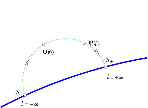
Figure 1: Convergence to stationary states.

All proofs rely on the analysis of radiation which irreversibly carries a portion of energy to infinity. The details can be found in the surveys [E8, E9].

In all the problems considered, the convergence (9.1) implies, by the Fatou theorem, the inequality

$${\cal H}(S_{\pm})\leq{\cal H}(Y(t))\equiv\mathop{\mathrm{const}}\nolimits,\,\,\,t\in\mathbb{R},$$ (9.7)

where $\mathcal{H}$ is the corresponding Hamiltonian (energy) functional. This inequality is an analog of the well-known property of weak convergence in Hilbert and Banach spaces. Simple examples show that the strict inequality in (9.7) is possible, which means that an irreversible scattering of energy to infinity occurs.

Example 9.1 (The d’Alembert waves).

In particular, the asymptotics (9.1) with the strict inequality (9.7) can easily be demonstrated for the d’Alembert equation $\ddot{\psi}(x,t)=\partial_{x}^{2}\psi(x,t)$ with general solution

$$\psi(x,t)=f(x-t)+g(x+t).$$ (9.8)

Indeed, the convergence $\psi(\cdot,t)\to 0$ in $L^{2}_{\mathrm{loc}}(\mathbb{R})$ obviously holds for all $f,g\in L^{2}(\mathbb{R})$. On the other hand, the convergence to zero in global norms obviously fails if $f(x)\not\equiv 0$ or $g(x)\not\equiv 0$.

Example 9.2 (Nonlinear Huygens Principle).

Consider solutions of 3D wave equation with a unit propagation velocity and initial data with support in a ball $|x|<R$. The corresponding solution is concentrated in spherical layers $|t|-R<|x|<|t|+R$. Therefore, the energy localized in any bounded region converges to zero as $t\to\pm\infty$, although its total energy remains constant. This convergence to zero is known as the strong Huygens principle. Thus, global attraction to stationary states (9.1) is a generalization of the strong Huygens principle to nonlinear equations. The difference is that for the linear wave equation, the limit is always zero, while for nonlinear equations the limit can be any stationary solution.

Remark 9.3.

The proofs in [E10] and [E14] rely on the relaxation of acceleration

$$\ddot{q}(t)\to 0,\qquad t\to\pm\infty$$ (9.9)

for solutions to the coupled system (9.4) and similarly for solutions to the Maxwell–Lorentz system. This relaxation was discovered about 100 years ago in classical electrodynamics and is known as the radiation damping; see [A12, Chapter 16]. The detailed account on early investigations of this problem by A. Sommerfeld, H. Poincaré, P. Dirac and others can be found in Chapter 3 of [E15], see also [A7].

However, a rigorous proof of the relaxation (9.9) is not so obvious. It first appeared in [E10] and [E14] under the Wiener condition on the particle charge density

$$\hat{\rho}(k):=\int e^{ikx}\rho(x)\,dx\neq 0,\qquad k\in\mathbb{R}^{3}.$$ (9.10)

This condition is an analogue of the ‘‘Fermi Golden Rule’’ first introduced by Sigal in the context of nonlinear wave and Schrödinger equations [J34]. The proof of the relaxation (9.9) relies on a novel application of the Wiener Tauberian theorem.

9.2 Group of translations $G=\mathbb{R}^{n}$

For generic translation-invariant equations, the conjecture (8.5) means the attraction of all finite-energy solutions to solitons:

$$\psi(x,t)\sim\psi_{\pm}(x-v_{\pm}t),\qquad t\to\pm\infty,$$ (9.11)

where the convergence holds in local seminorms of type $L^{2}(|x-v_{\pm}t|<R)$ with any $R>0$, i.e., in the comoving reference frame. A trivial example is provided by the d’Alembert equation $\ddot{\psi}(x,t)=\partial_{x}^{2}\psi(x,t)$ with general solution (9.8) corresponding to the asymptotics (9.11) with $v_{+}=\pm 1$ and $v_{-}=\pm 1$.

Such soliton asymptotics was first proved for completely integrable equations (Korteweg–de Vries equation, etc.); see [F1, F8]. Moreover, for the Korteweg–de Vries equation, more accurate soliton asymptotics in global norms with several solitons were discovered by Kruskal and Zabusky in 1965 by numerical simulation: it is the decay to solitons

$$\psi(x,t)\sim\sum_{k}\psi_{\pm}(x-v^{k}_{\pm}t)+w_{\pm}(x,t),\qquad t\to\pm\infty,$$ (9.12)

where $w_{\pm}$ are some dispersive waves.

Later on, such asymptotics were proved by the method of inverse scattering problem for nonlinear completely integrable Hamiltonian translation-invariant equations (Korteweg–de Vries, etc.) in the works of Ablowitz, Segur, Eckhaus, van Harten, and others [F1, F8].

For equations which are not completely integrable, the global attraction (9.11) was established in [F2]–[F7]. The first result was obtained in [F6] for the translation-invariant system (9.4) with zero external potential $V=0$. In this case the total momentum is conserved:

$$P:=p-\int\dot{\psi}(x,t)\nabla\psi(x,t)\,dx=\mathop{\mathrm{const}}\nolimits.$$ (9.13)

In [F2], the result was extended to the Maxwell–Lorentz system (9.6) with $V=0$. The proofs in [F6] and [F2] rely on variational properties of solitons and their orbital stability, as well as on the relaxation of the acceleration (9.9) under the Wiener condition (9.10). The case of small charge was considered in [F3, F4].

Let us mention that for non-completely-integrable equations the multi-soliton asymptotics (9.12) were observed numerically for 1D relativistically-invariant nonlinear wave equations in [F7].

9.3 Unitary symmetry group $G=\mathbf{U}(1)$

For generic $\mathbf{U}(1)$-invariant equations, the conjecture (8.5) means the attraction of all finite-energy solutions to ‘‘stationary orbits’’:

$$\psi(x,t)\sim\phi_{\pm}(x)e^{-i\omega_{\pm}t},\qquad t\to\pm\infty,$$ (9.14)

where $\omega_{\pm}\in\mathbb{R}$. Such asymptotics are similar to the Bohr transitions between stationary orbits (6.4) of the coupled Maxwell–Schrödinger equations. This asymptotics means that there is a global attraction to the solitary manifold formed by all stationary orbits (3.3). The asymptotics is considered in the local seminorms $L^{2}(|x|<R)$ with any $R>0$. The global attractor is a smooth manifold formed by the circles that are the orbits of the action of the symmetry group $\mathbf{U}(1)$, as is illustrated on Fig. 2.

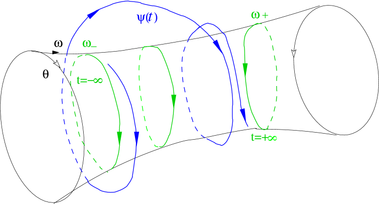
Figure 2: Convergence to stationary orbits.

Such an attraction was proved for the first time i) in [H1] and [H3]–[H9] for the Klein–Gordon and Dirac equations coupled to $\mathbf{U}(1)$-invariant nonlinear oscillators,

$$\ddot{\psi}(x,t) = \Delta\psi(x,t)-m^{2}\psi+\sum_{k=1}^{N}\rho(x-x_{k})F_{k}(\langle\psi(\cdot,t),\rho(\cdot-x_{k})\rangle),$$ (9.15)

$$i\dot{\psi}(x,t) = \big{(}-i\alpha\cdot\nabla+\beta m\big{)}\psi+\sum_{k=1}^{N}\rho(x-x_{k})F_{k}(\langle\psi(\cdot,t),\rho(\cdot-x_{k})\rangle),$$ (9.16)

under the Wiener condition (9.10), where $\alpha=(\alpha_{1},\dotsc,\alpha_{n})$ and $\beta=\alpha_{0}$ are the Dirac matrices; ii) in [H2] for a discrete approximations of such coupled systems, i.e. for the corresponding finite difference schemes; and iii) in [H11]–[H14] for the wave, Klein–Gordon, and Dirac equations with concentrated nonlinearities. More precisely, we have proved global attraction to the solitary manifold of all stationary orbits, although global attraction to particular stationary orbits (orbits with fixed $\omega_{\pm}$) is still an open problem.

All these results were proved under the assumption that the equations are ‘‘strictly nonlinear’’. For linear equations, the global attraction obviously fails if the discrete spectrum consists of at least two different eigenvalues.

The proofs of all these results rely on i) a nonlinear analog of the Kato theorem on the absence of embedded eigenvalues; ii) a new theory of multiplicators in the space of quasimeasures; iii) a novel application of the Titchmarsh convolution theorem [A10, A18, A27]. For application to the Klein–Gordon equation in discrete space-time (a numerical scheme) in [H2], the appropriate version of the Titchmarsh theorem is obtained in [H10].

The asymptotics (9.14) is closely related to the limiting amplitude principle [A16, A21] and to the theory of waveguides [A17].

9.4 Orthogonal group $G=\mathbf{SO}(3)$

For generic rotation-invariant equations, the conjecture (8.5) takes the form of the long-time asymptotics

$$\Psi(t)\sim e^{-i\hat{\Omega}_{\pm}t}\Psi_{\pm},\qquad t\to\pm\infty$$ (9.17)

for all finite-energy solutions, where $\hat{\Omega}_{\pm}$ are suitable representations of $\Omega_{\pm}\in\mathfrak{so}(3)$. This means that global attraction to ‘‘stationary $\mathbf{SO}(3)$-orbits’’ takes place. Such asymptotics for the Maxwell–Lorentz equations with a rotating particle are proved in [G5].

10  On generic equations

We must still specify the meaning of the term generic in our conjecture (8.5). In fact, this conjecture means that the asymptotics (8.5) hold for all solutions from an open dense set of $G$-invariant equations.
i) In particular, the asymptotics (9.1), (9.11), (9.14), and (9.17) hold under appropriate conditions, which define some ‘‘open dense subset’’ of $G$-invariant equations with the four types of the symmetry group $G$. This asymptotic expression may break down if these conditions fail: this corresponds to some ‘‘exceptional’’ equations. For example, the global attraction (9.14) breaks down for linear Schrödinger equations with at least two different eigenvalues. Thus, linear equations are exceptional, not generic!
ii) The general situation is as follows. Let the Lie group $G_{1}$ be a (proper) subgroup of some larger Lie group $G_{2}$. Then $G_{2}$-invariant equations form an ‘‘exceptional subset’’ among all $G_{1}$-invariant equations, and the corresponding asymptotics (8.5) may be completely different. For example, the trivial group $\{e\}$ is a proper subgroup in $\mathbf{U}(1)$ and in $\mathbb{R}^{n}$, and the asymptotic expressions (9.11) and (9.14) may differ significantly from (9.1).
iii) Examples of solitary wave solutions violating asymptotics (8.5) in particular non-generic models were constructed in [H8], [H6] (two-frequency solitary waves in models based on the Klein–Gordon equation with $\mathbf{U}(1)$-symmetry group), in [H2] (two- and four-frequency solitary waves in the discrete time-space Klein–Gordon equation with $\mathbf{U}(1)$-symmetry group), and in [I1] (two-frequency solitary waves in the Soler model with $\mathbf{SU}(1,1)$-symmetry group, when the solitary manifold is larger than the orbit of the action of $\mathbf{SU}(1,1)$).

11  Adiabatic effective dynamics of solitons

The system (9.4) admits soliton solutions

$$\phi_{v}(x-vt),\qquad q=vt$$ (11.1)

in the case of identically zero external potential $V(q)\equiv 0$. However, even in the case of nonzero external potential, soliton-like solutions of the form

$$\psi(x,t)\approx\psi_{v(t)}(x-q(t))$$ (11.2)

may exist if the potential is slowly varying:

$$|\nabla V(q)|\leq\varepsilon\ll 1.$$ (11.3)

In this case, the total momentum (9.13) is generally not conserved, but its slow evolution together with evolution of the parameters $q(t)$, $v(t)$ in (11.2) can be described in terms of an appropriate finite-dimensional Hamiltonian dynamics.

Indeed, denote by $P=P_{v}\in\mathbb{R}^{3}$ the total momentum (9.13) of the soliton (11.1). It is important that the map $\mathbf{P}:v\mapsto P_{v}$ is an isomorphism of the ball $|v|<1$ on $\mathbb{R}^{3}$. Therefore, we can consider $q,\,P$ as global coordinates on the solitary manifold

$$\mathcal{S}:=\{S_{q,v}=(\phi_{v}(x-q),-v\cdot\nabla\phi_{v}(x-q),a,v):q,v\in\mathbb{R}^{3},\,\,\,\,|v|<1\}.$$

The effective Hamiltonian functional is defined by

$$H_{\rm eff}(q,P_{v})\equiv H(S_{q,v}),\qquad q,\,P_{v}\in\mathbb{R}^{3},$$ (11.4)

where $H$ is the Hamiltonian (9.5) with $V(q)\equiv 0$. This functional can be represented as

$$H_{\rm eff}(Q,\Pi)=E(\Pi)+V(Q),$$

since the first integral in (9.5) does not depend on $Q$, while the last integral vanishes on the solitons. Hence, the corresponding Hamiltonian equations have the form

$$\dot{Q}(t)=\nabla E(\Pi(t)),\qquad\dot{\Pi}(t)=-\nabla V(Q(t)).$$ (11.5)

The main result in [G6] is the following theorem. Let us denote by $\|\cdot\|_{R}$ the norm in $L^{2}(B_{R})$, where $B_{R}$ is the ball $\{x\in\mathbb{R}^{3}:|x|<R\}$, and denote $\pi_{v}(x):=-v\nabla\phi_{v}(x)$.

Theorem 11.1.

Let the condition (11.3) hold, and assume that $(\psi(0),\,\dot{\psi}(0),\,q(0),\,p(0))\in\mathcal{S}$ is a soliton with the total momentum $P(0)$. Then the corresponding solution $(\psi(x,t),\,\dot{\psi}(x,t),\,q(t),\,p(t))$ of the system (9.4) with $V=0$ admits the ‘‘adiabatic asymptotics’’

$$|q(t)-Q(t)|\leq C_{0},\quad|P(t)-\Pi(t)|\leq C_{1}\varepsilon\quad\mbox{\rm for}\quad|t|\leq C\varepsilon^{-1},$$

$$\sup_{t\in\mathbb{R}}\Big{[}\|\nabla\psi(q(t)+y,t)-\nabla\psi_{v(t)}(y)]\|_{R}+\|\dot{\psi}(q(t)+y,t)-\pi_{v(t)}(y)\|_{R}\Big{]}\leq C\varepsilon,$$

where $P(t)$ denotes the total momentum (9.13), $v(t)=\mathbf{P}^{-1}(\Pi(t))$, and $(Q(t),\Pi(t))$ is the solution of the effective Hamiltonian equations (11.5) with initial conditions

$$Q(0)=q(0),\qquad\Pi(0)=P(0).$$

We note that such relevance of the effective dynamics (11.5) is due to the consistency of Hamiltonian structures:
I. The effective Hamiltonian (11.4) is the restriction of the Hamiltonian functional (9.5) with $V=0$ to the solitary manifold $\mathcal{S}$.
II. As shown in [G6], the canonical differential form of the Hamiltonian system (11.5) is also the restriction to $\mathcal{S}$ of the canonical differential form of the system (9.4): formally,

$$P\cdot dQ=\Bigl{[}p\cdot dq+\int\pi(x)\,d\psi(x)\,dx\Bigr{]}\Big{|}_{\mathcal{S}}.$$

Therefore, the total momentum $\mathbf{P}$ is canonically conjugate to the variable $Q$ on the solitary manifold $\mathcal{S}$. This fact justifies the definition (11.4) of the effective Hamiltonian as a function of the total momentum $P_{v}$, and not of the particle momentum $p_{v}$.

One of the important results in [G6] is the following ‘‘effective dispersion relation’’:

$$E(\Pi)\sim\frac{\Pi^{2}}{2(1+m_{e})}+{\rm const},\qquad|\Pi|\ll 1.$$ (11.6)

It means that the nonrelativistic mass of a slow soliton increases, due to the interaction with the field, by the amount

$$m_{e}=-\frac{1}{3}\langle\rho,\Delta^{-1}\rho\rangle.$$ (11.7)

This increment is proportional to the field energy of the soliton at rest,

$$E_{\rm own}=H(\Delta^{-1}\rho,0,0,0)=-\frac{1}{2}\langle\rho,\Delta^{-1}\rho\rangle,$$ (11.8)

which agrees with the Einstein mass-energy equivalence principle (see Section 11.1 below).

Remark 11.2.

The relation (11.6) suggests that $m_{e}$ is an increment of the effective mass. The true dynamical justification for such an interpretation is given by Theorem 11.1 which demonstrates the relevance of the effective dynamics (11.5).

Generalizations. In [G7], Kunze and Spohn extended Theorem 11.1 to solitons of the Maxwell–Lorentz equations (9.6) with slowly varying potential (11.3). Following the articles [G6, G7], suitable adiabatic effective dynamics was obtained in [G3] and [G4] for nonlinear Hartree and Schrödinger equations with slowly varying external potentials, and in [G2, G8] and [G9] for the nonlinear equations of Einstein–Dirac, Chern–Simon–Schrödinger and Klein–Gordon–Maxwell with small external fields. In [G5], the adiabatic effective dynamics was established for the Maxwell–Lorentz equations with a rotating particle. Similar adiabatic effective dynamics was established in [G1] for an electron in the second-quantized Maxwell field in the presence of a slowly varying external potential. The results of numerical simulation [F7] confirm the adiabatic effective dynamics of solitons for relativistic 1D nonlinear wave equations (see Section 14).

11.1 Mass-energy equivalence

In [G7], Kunze and Spohn have established that in the case of the Maxwell–Lorentz equations (9.6) with slowly varying potential (11.3), the increment of nonrelativistic mass also turns out to be proportional to the energy of the static soliton’s own field. Such an equivalence of the self-energy of a particle with its mass was first discovered in 1902 by M. Abraham: he showed by direct calculation that the energy $E_{\rm own}$ of electrostatic field of an electron at rest adds

$$m_{e}=\displaystyle\frac{4}{3}E_{\rm own}/c^{2}$$ (11.9)

to its nonrelativistic mass (see [A1, A2], and also [A13, pp. 216–217]). By (11.8), this self-energy is infinite for a point particle with the charge density $\rho(x)=\delta(x)$. This means that the field mass for a point electron is infinite, which contradicts experiments. That is why M. Abraham introduced the model of electrodynamics with extended electron (9.6), whose self-energy is finite.

At the same time, M. Abraham conjectured that the entire mass of an electron is due to its own electromagnetic energy, i.e., $m=m_{e}$: ‘‘matter disappeared, only energy remains’’, as philosophically-minded contemporaries wrote [A11, pp. 63, 87, 88]. (smile :))

In 1905, the formula (11.9) was corrected by A. Einstein, who discovered the famous universal relation $E=m_{0}c^{2}$ which follows from the Special Theory of Relativity [A8]. Thus, Abraham’s discovery of the mass-energy equivalence anticipated Einstein’s theory. The doubtful factor $\frac{4}{3}$ in Abraham’s formula is due to the nonrelativistic character of the system (9.6). According to the modern view, about 80% of the electron mass is of electromagnetic origin [A9].

12  Stability of stationary orbits and solitons

In 1987–1990, Grillakis, Shatah and Strauss developed general theory of orbital stability of the solitary waves [I7]. In [J2], Bambusi and Galgani established orbital stability of solitons for the Maxwell–Lorentz system (9.6).

Asymptotic stability of solitary manifold has the meaning of the local attraction, i.e., the convergence to this manifold of states that were sufficiently close to it. The first results of such type were obtained by Morawetz, Segal, and Strauss in the case when the attractor consists of the single point zero. In this case, the attraction is called local energy decay [C1]–[C7].

In the case of a continuous attractor, the key peculiarity of this convergence is the instability of the dynamics along the manifold. The instability follows directly from the fact that solitons move with different speeds and therefore run away for large times. Analytically, this instability is caused by the presence of the Jordan block corresponding to eigenvalue $\lambda=0$ in the spectrum of the generator of linearized dynamics. The tangent vectors to the soliton manifold are eigenvectors and generalized eigenvectors corresponding to this Jordan block. Thus, Lyapunov’s theory is not applicable to this case.

Remark 12.1.

According to Arnold (see e.g. [A3] and references therein), a similar instability mechanism may be responsible for the mixing and ergodicity of the turbulent flows.

In a series of articles published during 1985–2003, Weinstein, Soffer, Buslaev, Perelman, and Sulem discovered an original strategy for proving asymptotic stability of solitary manifolds. This strategy relies on i) special projection of a trajectory onto the solitary manifold, ii) modulation equations for parameters of the projection, and iii) time decay of the transversal component. This approach is a far-reaching development of the Lyapunov stability theory.

12.1 Spectral stability of solitons

Spectral (or linear) stability of solitary waves can be traced back to 1967, to the work of Zakharov [I19] on nonlinear Schrödinger equation

$$i\dot{\psi}=-\Delta\psi-|\psi|^{2}\psi,\qquad\psi(x,t)\in\mathbb{C},\quad x\in\mathbb{R}^{n},\quad n\geq 1,$$ (12.1)

which was later developed by Kolokolov [I8]. This is the ‘‘weakest’’ type of stability: one considers the perturbation of a solitary wave solution $\phi(x)e^{-i\omega t}$, $\phi(x)\in\mathbb{R}$, in the form of the Ansatz

$$\psi(x,t)=(\phi(x)+\chi(x,t))e^{-i\omega t},$$

with complex-valued perturbation $\chi(x,t)=u(x,t)+iv(x,t)$ (with $u,\,v$ real-valued), which is assumed to be small at $t=0$. Then one derives the linear approximation to the evolution of $\chi$, of the form

$$\frac{\partial}{\partial t}\begin{bmatrix}u\\ v\end{bmatrix}=A\begin{bmatrix}u\\ v\end{bmatrix},$$ (12.2)

and studies the spectrum of the operator $A=\begin{bmatrix}0&L_{0}\\ -L_{1}&0\end{bmatrix}$, where

$$L_{0}=-\Delta-\phi^{2}+\omega,\qquad L_{1}=-\Delta-3\phi^{2}+\omega$$

are the Schrödinger-type operators. One can show that in the case $n\leq 2$ one has $\sigma(A)\subset i\mathbb{R}$ (and the corresponding solitary wave is called spectrally stable), while for $n\geq 3$ the intersection $\sigma(A)\cap(0,+\infty)$ contains a positive eigenvalue (the corresponding solitary wave is called linearly unstable). We note that the system (12.2) can not be written as a $\mathbb{C}$-linear equation on $\chi$: in the Physics terminology, the $\mathbf{U}(1)$-symmetry is broken by the choice $\phi(x)\in\mathbb{R}$.

In the context of the nonlinear Schrödinger and Klein–Gordon equations and similar systems the spectral stability has been extended to orbital stability; see [I6, I7, I10, I18]. At the same time, the orbital stability for the nonlinear Dirac equation, and likewise for the Dirac–Maxwell and Dirac–Klein–Gordon systems, does not seem possible except via the proof of asymptotic stability, with the exception of the completely integrable massive Thirring model in one spatial dimension [I13]. Let us mention that the spectral stability for the nonlinear Dirac equation in the charge-subcritical cases has been proved in [I2] (see also [I3]).

12.2 Asymptotic stability of stationary orbits. Orthogonal projection

This strategy was formed in 1985–1992 in the pioneering work of Soffer and Weinstein [I11, I12, I18]; see the review [I17]. The results concern nonlinear $\mathbf{U}(1)$-invariant Schrödinger equations with real-valued potential $V(x)$,

$$i\dot{\psi}(x,t)=-\Delta\psi(x,t)+V(x)\psi(x,t)+\lambda|\psi(x,t)|^{p}\psi(x,t),\qquad x\in\mathbb{R}^{n},$$ (12.3)

where $\lambda\in\mathbb{R}$, $p=3$ or $4$, $n=2$ or $n=3$, and $\psi(x,t)\in\mathbb{C}$. The corresponding Hamiltonian functional is given by

$$\mathcal{H}=\int\Big{[}\frac{1}{2}|\nabla\psi(x)|^{2}+\frac{1}{2}V(x)|\psi(x)|^{2}+\frac{\lambda}{p}|\psi(x)|^{p}\Big{]}\,dx.$$

For $\lambda=0$, equation (12.3) is linear. Let $\phi_{*}(x)$ denote its ground state corresponding to the minimal eigenvalue $\omega_{*}<0$. Then $C\phi_{*}(x)e^{-i\omega_{*}t}$ are periodic solutions for any complex constant $C$. Corresponding phase curves are circles filling the complex plane. For nonlinear equations (12.3) with a small real $\lambda\neq 0$, it turns out that a wonderful bifurcation occurs: small neighborhood of zero in the complex plane turns into an analytic soliton manifold $\mathcal{S}$ invariant with respect to the dynamics group corresponding to (12.3), which is still filled with invariant circles $\phi_{\omega}(x)e^{-i\omega t}$ whose frequencies $\omega$ are close to $\omega_{*}$.

The main result of [I11, I12] (see also [I14]) is long-time attraction to one of these circles for any solution with sufficiently small initial data:

$$\psi(x,t)=\phi_{\pm}(x)e^{-i\omega_{\pm}t}+r_{\pm}(x,t),$$ (12.4)

where the remainder decay in weighted norms: for any $\sigma>2$,

$$\|\langle x\rangle^{-\sigma}r_{\pm}(\cdot,t)\|_{L^{2}(\mathbb{R}^{n})}\to 0,\qquad t\to\pm\infty,$$

where $\langle x\rangle:=(1+|x|)^{1/2}$. The proof relies on linearization of the dynamics and decomposition of solutions into two components,

$$\psi(t)=e^{-i\Theta(t)}(\phi_{\omega(t)}+\chi(t)),$$

satisfying the following orthogonality condition [I11, (3.2) and (3.4)]:

$$\langle\phi_{\omega(t)},\chi(t)\rangle=0.$$ (12.5)

This orthogonality and dynamics (12.3) imply the modulation equations for $\omega(t)$ and $\gamma(t)$, where $\gamma(t):=\Theta(t)-\displaystyle\int_{0}^{t}\omega(s)ds$ (see [I11, (3.9a)–(3.9b)]). The orthogonality (12.5) implies that the component $\phi(t)$ lies in the continuous spectral space of the Schrödinger operator

$$H(\omega_{0}):=-\Delta+V+\lambda|\phi_{\omega_{0}}|^{p},$$

which leads to the time decay of $\chi(t)$ (see [I11, (4.2a) and (4.2b)]). Finally, this decay implies the convergence $\omega(t)\to\omega_{\pm}$ and the asymptotics (12.4).

These results and methods were subsequently widely developed for the nonlinear Schrödinger, wave and Klein–Gordon equations with potentials under various spectral assumptions on linearized dynamics; see, for instance, [I15, I16].

12.3 Asymptotic stability of solitons. Symplectic projection

Next breakthrough in the theory of asymptotic stability was achieved in 1990–2003 by Buslaev, Perelman and Sulem [J5]–[J7], who first proved asymptotics of type (12.4) for translation-invariant 1D Schrödinger equations

$$i\dot{\psi}(x,t)=-\psi^{\prime\prime}(x,t)-F(\psi(x,t)),\qquad x\in\mathbb{R},$$ (12.6)

which are also assumed to be $\mathbf{U}(1)$-invariant, i.e., $F(\psi)=-\nabla U(\psi)$, and

$$F(e^{i\theta}\psi)=e^{i\theta}F(\psi),\qquad\psi\in\mathbb{C},\,\,\,\theta\in\mathbb{R}.$$ (12.7)

Moreover, they assume that

$$U(\psi)=\mathcal{O}(|\psi|^{10}),\qquad\psi\to 0.$$ (12.8)

Under some simple conditions on the potential $U$, there exist finite energy solutions of the form

$$\psi(x,t)=\phi_{0}(x)e^{i\omega_{0}t},$$ (12.9)

with $\omega_{0}>0$. The amplitude $\phi_{0}(x)$ satisfies the corresponding stationary equation

$$-\omega_{0}\phi_{0}(x)=-\phi_{0}^{\prime\prime}(x)-F(\phi_{0}(x)),\qquad x\in\mathbb{R},$$ (12.10)

which implies the ‘‘conservation law’’

$$\frac{|\phi_{0}^{\prime}(x)|^{2}}{2}+U_{e}(\phi_{0}(x))=E,$$ (12.11)

where the effective potential is given by $U_{e}(\psi)=U(\psi)+\omega_{0}\frac{|\psi|^{2}}{2}\sim\omega_{0}\frac{|\psi|^{2}}{2}$ as $\psi\to 0$ by (12.8). For the existence of a finite energy solution, the graph of ‘‘effective potential’’ $U_{e}(\psi)$ should be similar to Fig. 3. The finite energy solution $\phi_{0}(x)$ is defined by (12.11) with the constant $E=U_{e}(0)$ since for other $E$ the solutions to (12.11) do not converge to zero as $|x|\to\infty$. Equation (12.11) with $E=U_{e}(0)$ implies that

$$\frac{|\phi_{0}^{\prime}(x)|^{2}}{2}=U_{e}(0)-U_{e}(\phi_{0}(x))\sim\frac{\omega_{0}}{2}\phi_{0}^{2}(x).$$ (12.12)

Hence, for finite energy solutions, one has

$$\phi_{0}(x)\sim e^{-\sqrt{\omega_{0}}|x|},\qquad|x|\to\infty.$$ (12.13)

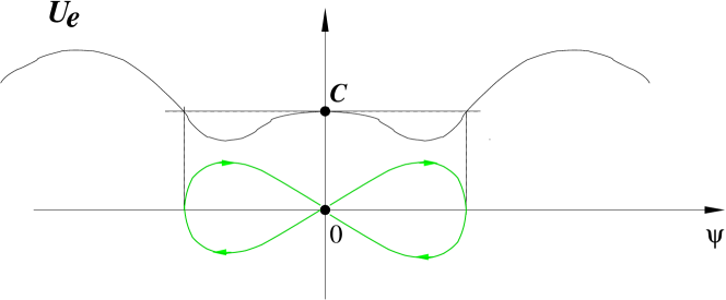
Figure 3: Reduced potential and soliton.

It is easy to verify that the following functions are also solutions (moving solitons):

$$\psi_{\omega,v,a,\theta}(x,t)=\phi_{\omega}(x-vt-a)e^{i(\omega t+kx+\theta)},\qquad\omega=\omega_{0}-v^{2}/4,\qquad k=v/2.$$ (12.14)

The set of all such solitons with parameters $\omega,v,a,\theta$ forms a 4-dimensional smooth submanifold $\mathcal{S}$ in the Hilbert phase space $\mathcal{X}:=L^{2}(\mathbb{R})$. Solitons (12.14) are obtained from (12.9) by the Galilean transformation

$$G(a,v,\theta):\psi(x,t)\mapsto\varphi(x,t)=\psi(x-vt-a,t)e^{i(-\frac{v^{2}}{4}t+\frac{v}{2}x+\theta)};$$ (12.15)

the Schrödinger equation (12.6) is invariant with respect to this group of transformations.

Linearization of the Schrödinger equation (12.6) at the soliton (12.9) is obtained as in Section 12.1, by substitution $\psi(x,t)=(\phi_{0}(x)+\chi(x,t))e^{i\omega_{0}t}$ and retaining terms of the first order in $\chi$. The resulting equation is not linear over the field of complex numbers, since it contains both $\chi$ and $\overline{\chi}$. This follows from the fact that the nonlinearity $F(\psi)=a(|\psi|^{2})\psi$ is not complex-analytic due to the $\mathbf{U}(1)$-invariance (12.7). Complexification of this linearized equation reads as follows:

$$\dot{\Psi}(x,t)=A_{0}\Psi(x,t),\qquad A_{0}=-jH_{0},$$ (12.16)

where $j$ is a real $2\times 2$ matrix, representing the multiplier $i$, $\Psi(x,t)\in\mathbb{C}^{2}$, and $H_{0}=-{d^{2}}/{dx^{2}}+\omega_{0}+V(x)$, where $V(x)$ is a real, matrix-valued potential which decreases exponentially as $|x|\to\infty$ due to (12.13). Note that the operator $A_{0}$ in (12.16) corresponds to the linearization at the soliton (12.14) with parameters $\omega=\omega_{0}$ and $a=v=\theta=0$. Similar operators $A(\omega,a,v,\theta)$ corresponding to linearization at solitons (12.14) with various parameters $\omega,a,v,\theta$ are also connected by the linear Galilean transformation (12.15). Therefore, their spectral properties completely coincide. In particular, their continuous spectra coincide with $(-i\infty,-i\omega_{0}]\cup[i\omega_{0},i\infty)$.

Main results of [J5]–[J7] are asymptotics of type (12.4) for solutions with initial data close to the solitary manifold $\mathcal{S}$:

$$\psi(x,t)=\phi_{\pm}(x-v_{\pm}t)e^{-i(\omega_{\pm}t+k_{\pm}x)}+W(t)\Phi_{\pm}+r_{\pm}(x,t),\qquad\pm t>0,$$ (12.17)

where $W(t)$ is the dynamical group of the free Schrödinger equation, $\Phi_{\pm}$ are some scattering states of finite energy, and $r_{\pm}$ are remainder terms which decay to zero in the global norm:

$$\|r_{\pm}(\cdot,t)\|_{L^{2}(\mathbb{R})}\to 0,\qquad t\to\pm\infty.$$ (12.18)

These asymptotics were obtained under the following assumptions on the spectrum of the generator $B_{0}$:

U1. The discrete spectrum of the operator $C_{0}$ consists of exactly three eigenvalues $0$ and $\pm i\lambda 0$, and

$$\lambda<\omega_{0}<2\lambda.$$ (12.19)

This condition means that the discrete mode interacts with the continuous spectrum already in the first order of approximation.

U2. The edge points $\pm i\omega_{0}$ of the continuous spectrum are neither eigenvalues, nor virtual levels (threshold resonances) of $C_{0}$.

U3. Furthermore, it is assumed the condition [J7, (1.0.12)], which means a strong coupling of discrete and continuous spectral components, providing energy radiation, similarly to the Wiener condition [A14, (6.24)], [E9, (1.5.13)]. It ensures that the interaction of discrete component with continuous spectrum does not vanish already in the first order of perturbation theory.

This condition is a nonlinear version of the Fermi Golden Rule [A23], which was introduced by Sigal in the context of nonlinear PDEs [J34].

Examples of potentials satisfying all these conditions are constructed in [J19].

In 2001, Cuccagna extended results of [J5]–[J7] to translation-invariant Schrödinger equations in $\mathbb{R}^{n}$, $n\geq 2$ [J9]. Similar approach to the asymptotic stability of solitons was developed for the Korteweg–de Vries equation in [J30], for the regularized long-wave equation in [J29], and for the nonlinear Schrödinger equation in $\mathbb{R}^{3}$ with concentrated nonlinearity in [J1]. In the context of the nonlinear Dirac equation with a potential, stability with respect to perturbations of solitary waves in particular directions was considered in [I5].

Method of symplectic projection in the Hilbert phase space. Novel approach [J5]–[J7] relies on symplectic projection $P$ of solutions onto the solitary manifold. This means that

$$Z:=\psi-S\quad\mbox{symplectic-orthogonal to the tangent space}\quad\mathcal{T}:=T_{S}\mathcal{S}$$

for the projection $S:=P\psi$. This projection is correctly defined in a small neighborhood of $\mathcal{S}$. For this it is important that $\mathcal{S}$ is a symplectic manifold, i.e. the corresponding symplectic form is non-degenerate on the tangent spaces $T_{S}\mathcal{S}$.

In particular, the approach [J5]–[J7] allowed to get rid of the assumption that the initial data are small.

Now a solution $\psi(t)$ for each $t>0$ decomposes onto symplectic-orthogonal components $\psi(t)=S(t)+Z(t)$, where $S(t):=P\psi(t)$, and the dynamics is linearized on the soliton $S(t)$.

The Hilbert phase space $\mathcal{X}:=L^{2}(\mathbb{R})$ is split as $\mathcal{X}=\mathcal{T}(t)\oplus\mathcal{Z}(t)$, where ${\mathcal{Z}}(t)$ is symplectic-orthogonal complement to the tangent space $\mathcal{T}(t):=T_{S(t)}\mathcal{S}$. The corresponding equation for the transversal component $Z(t)$ reads

$$\dot{Z}(t)=A(t)Z(t)+N(t),$$

where $A(t)Z(t)$ is the linear part, and $N(t)=\mathcal{O}(\|Z(t)\|^{2})$ is the corresponding nonlinear part. The main difficulties in studying this equation are as follows i) it is non-autonomous, and ii) the generators $A(t)$ are not self-adjoint (see Appendix in [J17]). It is important that $A(t)$ are Hamiltonian operators, for which the existence of spectral decomposition is provided by the Krein–Langer theory of $J$ -selfadjoint operators [J24, J25]. In [J17, J18] we have developed a special version of this theory providing the corresponding eigenfunction expansion which is necessary for the justification of the approach [J5]–[J7].
The main steps of the strategy [J5]–[J7] are as follows:

$\bullet$ Modulation equations. The parameters of the soliton $S(t)$ satisfy modulation equations: for example, for the speed $v(t)$ we have

$$\dot{v}(t)=M(\psi(t)),$$

where $M(\psi)=\mathcal{O}(\|Z\|^{2})$ for small norms $\|Z\|$. Therefore, the parameters change ‘‘super-slow’’ near the soliton manifold, like adiabatic invariants.

$\bullet$ Tangent and transversal components. The transversal component $Z(t)$ in the splitting $\psi(t)=S(t)+Z(t)$ belongs to the transversal space $\mathcal{Z}(t)$. The tangent space $\mathcal{T}(t)$ is the root space of the generator $A(t)$ and corresponds to the ‘‘unstable’’ spectral point $\lambda=0$. The key observation is that

i) symplectic-orthogonal subspace ${\mathcal{Z}}(t)$ does not contain ‘‘unstable’’ tangent vectors, and, moreover,

ii) the subspace ${\mathcal{Z}}(t)$ is invariant with respect to the generator $A(t)$, since the subspace $\mathcal{T}(t)$ is invariant, and $A(t)$ is the Hamiltonian operator.

$\bullet$ Continuous and discrete components. The transversal component allows further splitting $Z(t)=z(t)+f(t)$, where $z(t)$ and $f(t)$ belong, respectively, to discrete and continuous spectral subspaces $\mathcal{Z}_{d}(t)$ and $\mathcal{Z}_{c}(t)$ of $A(t)$ in the space $\mathcal{Z}(t)=\mathcal{Z}_{d}(t)+\mathcal{Z}_{c}(t)$.

$\bullet$ Poincare normal forms and Fermi Golden Rule. The component $z(t)$ satisfies a nonlinear equation, which is reduced to Poincare normal form up to higher order terms [J7, Equations (4.3.20)]. (For the relativistic-invariant Ginzburg–Landau equation, a similar reduction done in [J23, Equations (5.18)].) The normal form allowed to derive some ‘‘conditional’’ decay for $z(t)$ using the Fermi Golden Rule [J7, (1.0.12)].

$\bullet$ Method of majorants. A skillful combination of the conditional decay for $z(t)$ with super-slow evolution of the soliton parameters allows us to prove the decay for $f(t)$ and $z(t)$ by the method of majorants. Finally, this decay implies the asymptotics (12.17)–(12.18).

12.4 Generalizations and Applications

$N$-soliton solutions. The methods and results of [J7] were developed in [J26]–[J28] and [J31]–[J33] for $N$-soliton solutions for translation-invariant nonlinear Schrödinger equations.

Multiphoton radiation. In [J10], Cuccagna and Mizumachi extended methods and results of [J7] to the case when the inequality (12.19) is changed to

$$N\lambda<\omega_{0}<(N+1)\lambda,$$

with some natural $N>1$, and the corresponding analogue of condition U3 holds. It means that the interaction of discrete modes with a continuous spectrum occurs only in the $N$-th order of perturbation theory. The decay rate of the remainder term (12.18) worsens with growing $N$.

Linear equations coupled to nonlinear oscillators and particles. In [I4, I9] methods and results of [J7] were extended to i) the Schrödinger equation interacting with a nonlinear $\mathbf{U}(1)$– invariant oscillator, ii) in [J14, J15]– to translation-invariant systems of relativistic particle coupled to the wave and Maxwell equations, and iii) in [J13, J16, J20]– to similar translation-invariant systems of relativistic particle coupled to the Klein–Gordon, Schrödinger and Dirac equations. The review of the results [J13]–[J15] can be found in [J12].

Relativistic equations. In [J3, J4, J21, J22, J23] methods and results [J7] were extended for the first time to relativistic-invariant nonlinear equations. Namely, i) in [J3] and [J21]–[J23] asymptotics of type (12.17) were obtained for 1D relativistic-invariant nonlinear wave equations with potentials of the Ginzburg–Landau type,

$$\ddot{\psi}(x,t)=\Delta\psi(x,t)-m^{2}\psi(x,t)+f(\psi(x,t)),$$ (12.20)

and ii) in [J4] and [J8] for relativistic-invariant nonlinear Dirac equations. In [J19] we have constructed examples of potentials providing all spectral properties of the linearized dynamics imposed in [J21]–[J23].

The justification of the eigenfunction expansions. In [J17, J18] we have justified the eigenfunction expansions for nonselfadjoint Hamiltonian operators which were used in [J21]–[J23]. For the justification we have developed a special version of the Krein–Langer theory of $J$ -selfadjoint operators [J24, J25]

Vavilov–Cherenkov radiation. The article [J11] concerns the nonrelativistic particle coupled to the Schrödinger equation (system (1.9)–(1.10) in [J11]). This system is considered as a model of the Cherenkov radiation. The main result of [J11] is long-time convergence to a soliton with the sonic speed for initial solitons with a supersonic speed in the case of a weak interaction (‘‘Bogoliubov limit’’) and small initial field.

Asymptotic stability of solitons for similar system was established in [J16].

12.5 Further generalizations

The results on asymptotic stability of solitons were developed in different directions.

Systems with several bound states. The case of many simple eigenvalues of linearization at a soliton (12.16) was first investigated in [K1]–[K5] for the nonlinear Schrödinger equation

$$i\dot{\psi}(x,t)=(-\Delta+V(x))\psi(x,t)\pm|\psi(x,t)|^{2}\psi(x,t),\qquad x\in\mathbb{R}^{3}.$$

Asymptotic stability and long-time asymptotics of solutions were established under the following assumptions:

i) the endpoint of the essential spectrum is neither an eigenvalue nor a virtual level (threshold resonance) for linearized equation;

ii) the eigenvalues of the linearized equation satisfy the corresponding non-resonance condition;

iii) a new version of the Fermi Golden Rule.

The main obtained result: any solution with small initial data converges to some ground state at $t\to\infty$ with speed $t^{-1/2}$ in $L^{2}_{\rm loc}(\mathbb{R}^{3})$. There are different long-time regimes depending on relative contributions of eigenfunctions into initial data.

One of the difficulties is the possible existence of invariant tori corresponding to the resonances. Great efforts have been applied to show that the role of metastable tori decays like $t^{-1/2}$ as $t\to\infty$.

This result was extended in [K1] to nonlinear Klein–Gordon equations

$$\ddot{\psi}(x,t)=(\Delta-V(x)-m^{2})\psi(x,t)+f(\psi(x,t)),\qquad x\in\mathbb{R}^{3}.$$

Namely, under conditions i) – iii) above, any sufficiently small solution for large times asymptotically is a free wave in the norm $H^{1}(\mathbb{R}^{3})$. The proofs largely rely on the theory of the Birkhoff normal forms. The main novelty is the transition to normal forms without loss of the Hamiltonian structure.

In [K2] the results of [J10, K1] are extended to nonlinear Schrödinger equation

$$i\dot{\psi}(x,t)=(-\Delta+V(x))\psi(x,t)+\beta(|\psi(x,t)|)\psi(x,t),\qquad x\in\mathbb{R}^{3}.$$

Main results are long-time asymptotics ‘‘ground state + dispersive wave’’ in the norm $H^{1}(\mathbb{R}^{3})$ for solutions close to the ground state.

The corresponding linearized equation can have many eigenvalues, which must satisfy the non-resonant conditions [K1], and suitable modification of the Fermi Golden Rule holds. However, for nonlinear Schrödinger equations methods of [K1] required a significant improvement: now the canonical coordinates are constructed using the Darboux theorem.

General theory of relativity. The article [L4] concerns so-called ‘‘kink instability’’ of self-similar and spherically symmetric solutions of the equations of the general theory of relativity with a scalar field, as well as with a ‘‘hard fluid’’ as sources. The authors constructed examples of self-similar solutions that are unstable to the kink perturbations.

The article [L2] examines linear stability of slowly rotating Kerr solutions for the Einstein equations in vacuum. In [L5] a pointwise damping of solutions to the wave equation is investigated for the case of stationary asymptotically flat space-time in the three-dimensional case.

In [L1] the Maxwell equations are considered outside slowly rotating Kerr black hole. The main results are: i)   boundedness of a positive definite energy on each hypersurface $t=\mathop{\mathrm{const}}\nolimits$ and ii) convergence of each solution to a stationary Coulomb field.

In [L3] the pointwise decay was proved for linear waves against the Schwarzschild black hole.

Method of concentration compactness. In [M4] the concentration compactness method was used for the first time to prove global well-posedness, scattering and blow-up of solutions to critical focusing nonlinear Schrödinger equation

$$i\dot{\psi}(x,t)=-\Delta\psi(x,t)-|\psi(x,t)|^{\frac{4}{n-2}}\psi(x,t),\qquad x\in\mathbb{R}^{n}$$

in the radial case. Later on, these methods were extended in [M1, M3, M5, M9] to general non-radial solutions and to nonlinear wave equations of the form

$$\ddot{\psi}(x,t)=\Delta\psi(x,t)+|\psi(x,t)|^{\frac{4}{n-2}}\psi(x,t),\qquad x\in\mathbb{R}^{n}.$$

One of the main results is splitting of the set of initial states, close to the critical energy level, into three subsets with certain long-term asymptotics: either a blow-up in a finite time, or an asymptotically free wave, or the sum of the ground state and an asymptotically free wave. All three alternatives are possible; all nine combinations with $t\to\pm\infty$ are also possible. Lectures [M11] give excellent introduction to this area. The articles [M2, M6] concern super-critical nonlinear wave equations.

Recently, these methods and results were extended to critical wave mappings [M7]–[M10]. The ‘‘decay onto solitons’’ is proved: every $1$-equivariant finite-energy wave mapping of exterior of a ball with Dirichlet boundary conditions into three-dimensional sphere exists globally in time and dissipates into a single stationary solution of its own topological class.

13  Linear dispersion

In all results on long-time asymptotic for nonlinear Hamiltonian PDEs, the key role is played by dispersive decay of solutions of the corresponding linearized equations. In this section, we choose most important or recent articles out of a huge number of publications.

Dispersion decay in weighted Sobolev norms. Dispersion decay for wave equations was first proved in linear scattering theory [N25]. For the Schrödinger equation with a potential, a systematic approach to dispersive decay was proposed by Agmon [N1] and Jensen and Kato [N12]. This theory was extended by many authors to wave, Klein–Gordon and Dirac equations and to the corresponding discrete equations, see [N3]–[N11], [N13]–[N24] and references therein.

$L^{1}$-$L^{\infty}$ decay for solutions of the linear Schrödinger equation was proved for the first time by Journé, Soffer, and Sogge [N13]. Namely, it was shown that the solutions to

$$i\dot{\psi}(x,t)=H\psi(x,t):=(-\Delta+V(x))\psi(x,t),\qquad x\in\mathbb{R}^{n},\qquad n\geq 3$$ (13.1)

satisfy

$$\|P_{c}\psi(t)\|_{L^{\infty}(\mathbb{R}^{n})}\leq Ct^{-n/2}\|\psi(0)\|_{L^{1}(\mathbb{R}^{n})},\qquad t>0,$$ (13.2)

provided that $\lambda=0$ is neither an eigenvalue nor a virtual level of $H$. Here $P_{c}$ is an orthogonal projection onto continuous spectral space of the operator $H$. It is assumed that the potential $V(x)$ is real-valued, sufficiently smooth, and rapidly decays as $|x|\to\infty$. This result was generalized later by many authors; see below.

The decay of type (13.2) and Strichartz estimates were established in [N27] for 3D Schrödinger equations (13.1) with ‘‘rough’’ and time-dependent potentials $V=V(x,t)$. Similar estimates were obtained in [N3] for 3D Schrödinger and wave equations with (stationary) Kato class potentials.

In [N7], the 4D Schrödinger equations (13.1) are considered in the case when there is a virtual level or an eigenvalue at zero energy. In particular, in the case of an eigenvalue at zero energy, there is a time-dependent operator $F_{t}$ of rank $1$ such that $\|F_{t}\|_{L^{1}\to L^{\infty}}\leq 1/\log t$ for $t>2$, and

$$\|e^{itH}P_{c}-F_{t}\|_{L^{1}\to L^{\infty}}\leq Ct^{-1},\qquad t>2.$$

Similar dispersive estimates were also proved for solutions to 4D wave equation with a potential.

In [N8, N9], the Schrödinger equation (13.1) is considered in $\mathbb{R}^{n}$ with $n\geq 5$ with the assumption that zero is an eigenvalue (the Schrödinger operator in dimension $n\geq 5$ could only have zero eigenvalues but no genuine virtual level at zero). It is shown, in particular, that there is a time-dependent rank one operator $F_{t}$ such that $\|F_{t}\|_{L^{1}\to L^{\infty}}\leq C|t|^{2-n/2}$ for $|t|>1$, and

$$\|e^{itH}P_{c}-F_{t}\|_{L^{1}\to L^{\infty}}\leq C|t|^{1-n/2},\qquad|t|>1.$$

With a stronger decay of the potential, the evolution admits an operator-valued expansion

$$e^{itH}P_{c}(H)=|t|^{2-n/2}A_{-2}+|t|^{1-n/2}A_{-1}+|t|^{-n/2}A_{0},$$

where $A_{-2}$ and $A_{-1}$ are finite rank operators $L^{1}(\mathbb{R}^{n})\to L^{\infty}(\mathbb{R}^{n})$, while $A_{0}$ maps weighted $L^{1}$ spaces to weighted $L^{\infty}$ spaces. The operators $A_{-2}$ and $A_{-1}$ are equal to zero under certain conditions of the orthogonality of the potential $V$ to the eigenfunction which corresponds to zero eigenvalue. Under the same orthogonality conditions, the remainder term $|t|^{-n/2}A_{0}$ also maps $L^{1}(\mathbb{R}^{n})$ to $L^{\infty}(\mathbb{R}^{n})$, and therefore the group $e^{itH}P_{c}(H)$ has the same dispersion decay as the free evolution, despite its eigenvalue at zero.

$L^{p}$-$L^{q}$ decay was first established in [N26] for solutions of the free Klein–Gordon equation $\ddot{\psi}=\Delta\psi-\psi$ with initial state $\psi(0)=0$:

$$\|\psi(t)\|_{L^{q}}\leq Ct^{-d}\|\dot{\psi}(0)\|_{L^{p}},\qquad t>1,$$ (13.3)

where $1\leq p\leq 2$, $1/p+1/q=1$, and $d\geq 0$ is a piecewise-linear function of $(1/p,1/q)$. The proofs use the Riesz interpolation theorem.

In [N2], the estimates (13.3) were extended to solutions of the perturbed Klein–Gordon equation

$$\ddot{\psi}=\Delta\psi-\psi+V(x)\psi$$

with $\psi(0)=0$. It is shown that (13.3) holds for $0\leq 1/p-1/2\leq 1/(n+1)$. The smallest value of $p$ and the fastest decay rate $d$ occurs when $1/p=1/2+1/(n+1)$, $d=(n-1)/(n+1)$. The result is proved under the assumption that the potential $V$ is smooth and small in a suitable sense. For example, the result holds true when $|V(x)|\leq c(1+|x|^{2})^{-\sigma}$, where $c>0$ is sufficiently small. Here $\sigma>2$ for $n=3$, $\sigma>n/2$ for odd $n\geq 5$, and $\sigma>(2n^{2}+3n+3)/4(n+1)$ for even $n\geq 4$. The results also apply to the case when $\psi(0)\neq 0$.

The seminal article [N13] concerns $L^{p}$-$L^{q}$ -decay of solutions to the Schrödinger equation (13.1). It is assumed that $(1+|x|^{2})^{\alpha}V(x)$ is a multiplier in the Sobolev spaces $H^{\eta}$ for some $\eta>0$ and $\alpha>n+4$, and the Fourier transform of $V$ belongs to $L^{1}(\mathbb{R}^{n})$. Under this conditions, the main result of [N13] is the following theorem: if $\lambda=0$ is neither an eigenvalue nor a virtual level of $H$, then

$$\|P_{c}\psi(t)\|_{L^{q}}\leq Ct^{-n(1/p-1/2)}\|\psi(0)\|_{L^{p}},\qquad t>1,$$ (13.4)

where $1\leq p\leq 2$ and $1/p+1/q=1$. Proofs are based on $L^{1}$-$L^{\infty}$-decay (13.2) and the Riesz interpolation theorem.

In [N28], under suitable conditions on the spatial decay of $V(x)$, the estimates (13.4) were proved for all $1\leq p\leq 2$ if $\lambda=0$ is neither an eigenvalue nor a virtual level of $H$, and for all $3/2<p\leq 2$ otherwise.

The Strichartz estimates were extended in [N6] to the Schrödinger equations with the magnetic field in $\mathbb{R}^{n}$ with $n\geq 3$; in [N5] – to the wave equations with a magnetic potential in $\mathbb{R}^{n}$ for $n\geq 3$; in [N4] – to the wave equation in $\mathbb{R}^{3}$ with potentials of the Kato class.

14  Numerical simulation of soliton asymptotics

Here we describe the results of Arkady Vinnichenko (1945-2009) on numerical simulation of i) global attraction to solitons (9.11) and (9.12), and ii) adiabatic effective dynamics of solitons for relativistic-invariant one-dimensional nonlinear wave equations [F7].

14.1 Kinks of relativistic-invariant Ginzburg–Landau equations

First, we simulated numerically solutions to relativistic-invariant 1D nonlinear wave equations with polynomial nonlinearity

$$\ddot{\psi}(x,t)=\psi^{\prime\prime}(x,t)+F(\psi(x,t)),$$ (14.1)

where $F(\psi)=-\psi^{3}+\psi$. Since $F(\psi)=0$ for $\psi=0,\,\pm 1$, there are three equilibrium states: $S(x)\equiv 0,\,+1,\,-1$.

The corresponding potential $U(\psi)=\frac{\psi^{4}}{4}-\frac{\psi^{2}}{2}+\frac{1}{4}$ has minima at $\psi=\pm 1$ and a local maximum at $\psi=0$, therefore two finite energy solutions $\psi={\pm 1}$ are stable, and the solution $\psi=0$ with infinite energy is unstable. Such potentials with two wells are called Ginzburg–Landau potentials.

Besides the constant stationary solutions $S(x)\equiv 0,+1,-1$, there is also a non-constant one, $S(x)=\tanh\frac{x}{\sqrt{2}}$, called a ‘‘kink’’. Its shifts and reflections $\pm S(\pm x-a)$ are also solutions, as well as their Lorentz transforms

$$\pm S(\gamma(\pm x-a-vt)),\qquad\gamma=1/{\sqrt{1-v^{2}}},\quad|v|<1.$$

These are uniformly moving ‘‘traveling waves’’ (i.e. solitons). The kink is strongly compressed when the velocity $v$ is close to $\pm 1$. Equation (14.1) is formally equivalent to the Hamiltonian system with the Hamiltonian

$$\mathcal{H}(\psi,\pi)=\int\Big{[}\frac{1}{2}|\pi(x)|^{2}+\frac{1}{2}|\psi^{\prime}(x)|^{2}+U(\psi(x))\Big{]}\,dx.$$ (14.2)

This Hamiltonian is finite for functions $(\psi,\pi)$ from the Hilbert space $\mathcal{E}=H^{1}(\mathbb{R}^{3})\oplus L^{2}(\mathbb{R}^{3})$, for which the convergence

$$\psi(x)\to\pm 1\quad\mbox{as}\quad|x|\to\pm\infty$$

is sufficiently fast.

Numerical simulation. Our numerical experiments show a decay of finite energy solutions to a finite set of kinks and dispersive waves that corresponds to the asymptotics of (9.12). One of the experiments is shown on Fig. 4: a finite energy solution to equation (14.1) decays into three kinks. Here the vertical line is the time axis, and the horizontal line is the space axis; the spatial scale redoubles at $t=20$ and at $t=60$. Red color corresponds to $\psi>1+\varepsilon$ values, blue color to $\psi<-1-\varepsilon$ values, and the yellow one to intermediate values $-1+\varepsilon<\psi<1-\varepsilon$, where $\varepsilon>0$ is sufficiently small. Thus, the yellow stripes represent the kinks, while the blue and red zones outside the yellow stripes are filled with dispersive waves. For $t=0$, the solution begins with a rather chaotic behavior, when there are no visible kinks. After 20 seconds, three separate kinks appear, which subsequently move almost uniformly.

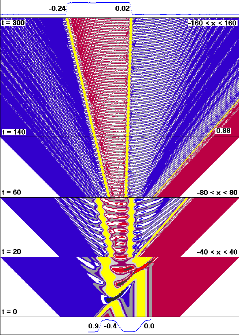
Figure 4: Decay to three kinks

The Lorentz contraction. The left kink moves to the left at a low speed $v_{1}\approx 0.24$, the central kink moves with a small velocity $v_{2}\approx 0.02$, and the right kink moves very fast with the speed $v_{3}\approx 0.88$. The Lorentz spatial contraction $\sqrt{1-v_{k}^{2}}$ is clearly visible on this picture: the central kink is wide, the left one is a bit narrower, and the right one is very narrow.

The Einstein time delay. Also, the Einstein time delay is also very prominent. Namely, all three kinks oscillate due to the presence of nonzero eigenvalue in the linearized equation at the kink: substituting $\psi(x,t)=S(x)+\varepsilon\varphi(x,t)$ in (14.1), we get in the first order of $\varepsilon$ the linearized equation

$$\ddot{\varphi}(x,t)=\varphi^{\prime\prime}(x,t)-2\varphi(x,t)-V(x)\varphi(x,t),$$ (14.3)

where the potential $V(x)=3S^{2}(x)-3=-\frac{3}{\cosh^{2}{x}/{\sqrt{2}}}$ decays exponentially for large $|x|$. It is of great convenience that for this potential the spectrum of the corresponding Schrödinger operator $H:=-\frac{d^{2}}{dx^{2}}+2+V(x)$ is well known [F8]. Namely, the operator $H$ is non-negative, and its continuous spectrum is given by $[2,\infty)$. It turns out that $H$ still has a two-point discrete spectrum: the points $\lambda=0$ and $\lambda=\frac{3}{2}$. Exactly this nonzero eigenvalue is responsible for the pulsations that we observe for the central slow kink, with the frequency $\omega_{2}\approx\sqrt{\frac{3}{2}}$ and period $T_{2}\approx 2\pi\sqrt{\frac{2}{3}}$. On the other hand, for fast kinks, the ripples are much slower, i.e., the corresponding period is longer. This time delay agrees numerically with the Lorentz formulas. These agreements qualitatively confirm the relevance of our numerical simulation.

Dispersive waves. The analysis of dispersive waves provides additional confirmation. Namely, the space outside the kinks on Fig. 4 is filled with dispersive waves, whose values are very close to $\pm 1$, with accuracy $0.01$. These waves satisfy with high accuracy the linear Klein–Gordon equation which is obtained by linearization of the Ginzburg–Landau equation (14.1) at the stationary solutions $\psi_{\pm}\equiv\pm 1$:

$$\ddot{\varphi}(x,t)=\varphi^{\prime\prime}(x,t)-2\varphi(x,t).$$

The corresponding dispersion relation $\omega^{2}=k^{2}+2$ determines the group velocities of high-frequency wave packets:

$$\omega^{\prime}(k)=\frac{k}{\sqrt{k^{2}+2}}=\pm\frac{\sqrt{\omega^{2}-2}}{\omega}.$$ (14.4)

These wave packets are clearly visible on Fig. 4 as straight lines whose propagation speeds converge to $\pm 1$. This convergence is explained by the high-frequency limit $\omega^{\prime}(k)\to\pm 1$ as $\omega\to\pm\infty$. For example, for dispersive waves emitted by central kink, the frequencies $\omega=\pm n\omega_{2}\to\pm\infty$ are generated by the polynomial nonlinearity in (14.1), see [E8] for details.

The nonlinearity in (14.1) is chosen exactly because of well-known spectrum of the linearized equation (14.3). In numerical experiments [F7] we have also considered more general nonlinearities of the Ginzburg–Landau type. The results were qualitatively the same: for ‘‘any’’ initial data, the solution decays for large times into a sum of kinks and dispersive waves. Numerically, this is clearly visible, but rigorous justification remains an open problem.

14.2 Numerical observation of soliton asymptotics

Besides the kinks, our numerical experiments [F7] have also resulted in the soliton-type asymptotics (9.12) and adiabatic effective dynamics for solutions to the 1D relativistically-invariant nonlinear wave equations (14.1) with $F(\psi)=-U^{\prime}(\psi)$ for the polynomial potentials

$$U(\psi)=a|\psi|^{2m}-b|\psi|^{2n},$$ (14.5)

where $a,\,b>0$ and $m>n=2,\,3,\,\dotsc$. Respectively,

$$F(\psi)=-2am|\psi|^{2m-2}\psi+2bn|\psi|^{2n-2}\psi.$$ (14.6)

The parameters $a,\,m,\,b,\,n$ were taken as follows:

$a$	$m$	$b$	$n$
1	3	0.61	2
10	4	2.1	2
10	6	8.75	5

We have considered various ‘‘smooth’’ initial functions $\psi(x,0),\dot{\psi}(x,0)$ with supports on the interval $[-20,20]$. The second order finite-difference scheme with $\Delta x,\sim 0.01$, $\Delta t\sim 0.001$ was employed. In all cases we have observed the asymptotics of type (9.12) with the numbers of solitons $0,1,3,5$ for $t>100$.

14.3 Adiabatic effective dynamics of relativistic solitons

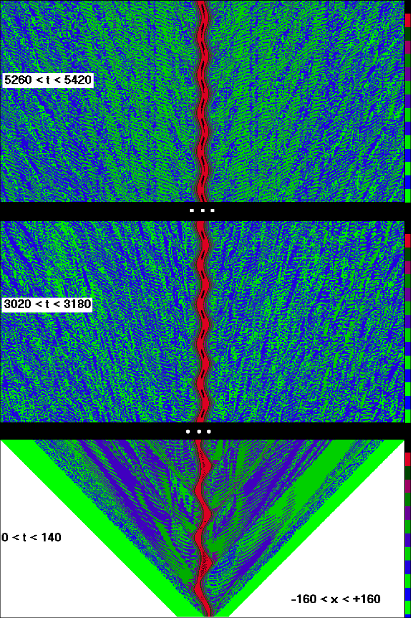
Figure 5: Adiabatic effective dynamics of relativistic solitons

In the numerical experiments [F7] we also observed the adiabatic effective dynamics for soliton-like solutions of the 1D equations with a slowly varying external potential $V(x)$:

$$\ddot{\psi}(x,t)=\psi^{\prime\prime}(x,t)-\psi(x,t)+F(\psi(x,t))-V(x)\psi(x,t),\qquad x\in\mathbb{R}.$$ (14.7)

This equation is formally equivalent to the Hamiltonian system with the Hamiltonian functional

$$\mathcal{H}_{V}(\psi,\pi)=\int\Big{[}\frac{1}{2}|\pi(x)|^{2}+\frac{1}{2}|\psi^{\prime}(x)|^{2}+U(\psi(x))+\frac{1}{2}V(x)|\psi(x)|^{2}\Big{]}\,dx.$$ (14.8)

The soliton-like solutions are of the form

$$\psi(x,t)\approx e^{i\Theta(t)}\phi_{\omega(t)}(\gamma_{v(t)}(x-q(t))).$$ (14.9)

Let us describe our numerical experiments which qualitatively confirm the adiabatic effective Hamiltonian dynamics for the parameters $\Theta,\,\omega,\,q$, and $v$, although its rigorous justification is still missing. The effective dynamics of such type is proved in [G1]–[G9] for several Hamiltonian models of PDEs coupled to a particle.

Figure 5 represents solutions to equation (14.7) with the potential (14.5) with $a=10$, $m=6$, $b=8.75$, and $n=5$. We choose

$$V(x)=-0.2\cos(0.31x)$$ (14.10)

and the following initial conditions:

$$\psi(x,0)=\phi_{\omega_{0}}(\gamma_{v_{0}}(x-q_{0})),\qquad\dot{\psi}(x,0)=0,$$ (14.11)

where $v_{0}=0$, $\omega_{0}=0.6$, and $q_{0}=5.0$. We note that the initial state does not belong to solitary manifold. The effective width (half-amplitude) of the solitons is in the range $[4.4,5.6]$. It is quite small compared to the spatial period of the potential $2\pi/0.31\sim 20$, which is confirmed by numerical simulations shown on Figure 5. Namely,
$\bullet$ Blue and green colors represent a dispersive wave with values $|\psi(x,t)|<0.01$, while red color represents a soliton with values $|\psi(x,t)|\in[0.4,0.8]$.
$\bullet$ The soliton trajectory (a thick red meandering curve) corresponds to oscillations of a classical particle in the potential $V(x)$.
$\bullet$ For $0<t<140$, the solution is far from the solitary manifold; the radiation is intense.
$\bullet$ For $3020<t<3180$, the solution approaches the solitary manifold; the radiation weakens. The oscillation amplitude of the soliton is almost unchanged for a long time, confirming Hamilton-type dynamics.
$\bullet$ However, for $5260<t<5420$, the amplitude of the soliton oscillation is halved. This suggests that at a large time scale the deviation from the Hamiltonian effective dynamics becomes essential. Consequently, the effective dynamics gives a good approximation only on the adiabatic time scale $t\sim\varepsilon^{-1}$.
$\bullet$ The deviation from the Hamiltonian dynamics is due to radiation, which plays the role of dissipation.
$\bullet$ The radiation is realized as dispersive waves bringing the energy to the infinity. The dispersive waves combine into uniformly moving bunches with discrete set of group velocities, as on Fig. 4. The magnitude of solutions is of order $\sim 1$ on the trajectory of the soliton, while the values of the dispersive waves is less than $0.01$ for $t>200$, so that their energy density does not exceed $0.0001$. The amplitude of the dispersive waves decays at large times. In the limit $t\to\pm\infty$, the soliton converges to a limit position which corresponds to a local minimum of the potential (14.10).

References

- [A1] M. Abraham, Prinzipien der Dynamik des Elektrons, Physikal. Zeitschr. 4 (1902), 57–63.
- [A2] M. Abraham, Theorie der Elektrizität, Bd.2: Elektromagnetische Theorie der Strahlung, Teubner, Leipzig, 1905.
- [A3] V.I. Arnold, B.S. Khesin, Topological Methods in Hydrodynamics, Springer, New York, 1998.
- [A4] N. Bohr, On the constitution of atoms and molecules, Phil. Mag. 26 (1913), 1–25, 476–502, 857–875.
- [A5] N. Bohr, Discussion with Einstein on epistemological problems in atomic physics, pp 201–241 in: Schilpp, P.A., Ed., Albert Einstein: Philosopher-Scientist Vol 7, Library of Living Philosophers, Evanston, Illinois, 1949.
- [A6] P. A. M. Dirac, The Principles of Quantum Mechanics, Oxford University Press, Oxford, 1999.
- [A7] P.A.M. Dirac, Classical theory of radiating electrons, Proc. Roy. Soc. A, 167 (1938), 148–169.
- [A8] A. Einstein, Ist die Trägheit eines Körpers von seinem Energieinhalt abhängig? Annalen der Physik 18 (1905), 639–643.
- [A9] R.P. Feynman, R.B. Leighton, M. Sands, The Feynman Lectures on Physics. Vol. 2: Mainly Electromagnetism and Matter, Addison-Wesley Publishing Co., Inc., Reading, Mass.-London, 1964.
- [A10] L. Hörmander, The Analysis of Linear Partial Differential Operators. I: Distribution theory and Fourier analysis, vol. 256 of Grundlehren der Mathematischen Wissenschaften, 2nd edition, Springer-Verlag, Berlin, 1990.
- [A11] L. Houllevigue, L’Évolution des Sciences, A. Collin, Paris, 1908.
- [A12] R.D. Jackson, Classical Electrodynamics, Wiley, New York, 1999.
- [A13] A. Komech, Quantum Mechanics: Genesis and Achievements, Springer, Dordrecht, 2013.
- [A14] A. Komech, Lectures on Quantum Mechanics and Attractors, World Scientific, Singapore, 2021.
- [A15] A. Komech, On quantum jumps and attractors of the Maxwell–Schrödinger equations, Annales mathématiques du Québec (2021), to appear.
- [A16] O.A. Ladyženskaya, On the principle of limit amplitude, Uspekhi Mat. Nauk 12 (1957), 161–164.
- [A17] L. Lewin, Advanced Theory of Waveguides, Iliffe and Sons, Ltd., London, 1951.
- [A18] B.Y. Levin, Lectures on Entire Functions, vol. 150 of Translations of Mathematical Monographs, American Mathematical Society, Providence, RI, 1996.
- [A19] L. Lusternik, L. Schnirelmann, Méthodes Topologiques dans les Problèmes Variationels, Hermann, Paris, 1934.
- [A20] L. Lusternik, L. Schnirelmann, Topological methods in variational problems and their applications to differential geometry of surfaces, Uspekhi Mat. Nauk 2 (1947), 166–217.
- [A21] C.S. Morawetz, The limiting amplitude principle, Comm. Pure Appl. Math. 15 (1962), 349–361.
- [A22] J. von Neumann, Mathematical Foundations of Quantum Mechanics, Princeton University Press Princeton, 1955.
- [A23] M. Reed, B. Simon, Methods of Modern Mathematical Physics. IV: Analysis of Operators, Academic Press, New York – London, 1978.
- [A24] W. Rudin, Functional Analysis, McGraw Hill, New York, 1977.
- [A25] E. Schrödinger, Quantisierung als Eigenwertproblem, Ann. d. Phys. I, II 79 (1926) 361, 489; III 80 (1926) 437; IV 81 (1926) 109. (English translations: E. Schrödinger, Collected Papers on Wave Mechanics, Blackie & Sohn, London, 1928.)
- [A26] V.I. Smirnov, A course of higher mathematics. II, Pergamon Press, 1964.
- [A27] E.C. Titchmarsh, The zeros of certain integral functions, Proc. London Math. Soc. S2-25 (1926), 283. B. Attractors of nonlinear dissipative PDEs
- [B1] A.V. Babin, M.I. Vishik, Attractors of Evolution Equations, vol. 25 of Studies in Mathematics and its Applications, North-Holland Publishing Co., Amsterdam, 1992.
- [B2] V.V. Chepyzhov, M.I. Vishik, Attractors of periodic processes and estimates of their dimensions, Math. Notes 57 (1995), 127–140.
- [B3] V.V. Chepyzhov, M.I. Vishik, Attractors for Equations of Mathematical Physics, vol. 49 of American Mathematical Society Colloquium Publications, American Mathematical Society, Providence, RI, 2002.
- [B4] V.V. Chepyzhov, V. Pata, M.I. Vishik, Averaging of nonautonomous damped wave equations with singularly oscillating external forces, Journal de Mathématiques Pures et Appliquées 90 (2008), no. 5, 469-491.
- [B5] C. Foias, O. Manley, R. Rosa, R. Temam, Navier–Stokes Equations and Turbulence, vol. 83 of Encyclopedia of Mathematics and its Applications, Cambridge University Press, Cambridge, 2001.
- [B6] J.K. Hale, Asymptotic Behavior of Dissipative Systems, vol. 25 of Mathematical Surveys and Monographs, American Mathematical Society, Providence, RI, 1988.
- [B7] A. Haraux, Systémes Dynamiques Dissipatifs et Applications, R.M.A. 17, Collection dirigé par Ph. Ciarlet et J.L. Lions, Masson, Paris, 1990.
- [B8] D. Henry, Geometric Theory of Semilinear Parabolic Equations, vol. 840 of Lecture Notes in Mathematics, Springer-Verlag, Berlin – New York, 1981.
- [B9] L. Landau, On the problem of turbulence, Doklady Acad. Sci. URSS 44 (1944), 311–314.
- [B10] R. Temam, Infinite-Dimensional Dynamical Systems in Mechanics and Physics, Springer, New York, 1997. C. Local energy decay
- [C1] C.S. Morawetz, Time decay for the nonlinear Klein–Gordon equations, Proc. Roy. Soc. Ser. A 306 (1968), 291–296.
- [C2] C.S. Morawetz, W.A. Strauss, Decay and scattering of solutions of a nonlinear relativistic wave equation, Comm. Pure Appl. Math. 25 (1972), 1–31.
- [C3] I. Segal, Quantization and dispersion for nonlinear relativistic equations, in Mathematical Theory of Elementary Particles (Proc. Conf., Dedham, Mass., 1965), M.I.T. Press, Cambridge, Mass., 1966, 79–108.
- [C4] I. Segal, Dispersion for non-linear relativistic equations. II, Ann. Sci. École Norm. Sup. (4) 1 (1968), 459–497.
- [C5] W.A. Strauss, Decay and asymptotics for , J. Functional Analysis 2 (1968), 409–457.
- [C6] W.A. Strauss, Nonlinear scattering theory at low energy, J. Funct. Anal. 41 (1981), 110–133.
- [C7] W.A. Strauss, Nonlinear scattering theory at low energy: sequel, J. Funct. Anal. 43 (1981), 281–293. D. Existence of stationary orbits and solitons
- [D1] H. Berestycki, P.-L. Lions, Nonlinear scalar field equations. I: Existence of a ground state, Arch. Rational Mech. Anal. 82 (1983), 313–345.
- [D2] H. Berestycki, P.-L. Lions, Nonlinear scalar field equations. II: Existence of infinitely many solutions, Arch. Rational Mech. Anal. 82 (1983), 347–375.
- [D3] G.M. Coclite, V. Georgiev, Solitary waves for Maxwell–Schrödinger equations, Electronic Journal of Differential Equations 94 (2004), 1–31.
- [D4] M.J. Esteban, V. Georgiev, E. Séré, Stationary solutions of the Maxwell–Dirac and the Klein–Gordon–Dirac equations, Calc. Var. Partial Differential Equations 4 (1996), 265–281.
- [D5] W.A. Strauss, Existence of solitary waves in higher dimensions, Comm. Math. Phys. 55 (1977), 149–162. E. Global attraction to stationary states
- [E1] A.V. Dymov, Dissipative effects in a linear Lagrangian system with infinitely many degrees of freedom, Izv. Math. 76 (2012), no. 6, 1116–1149.
- [E2] A. Komech, On the stabilization of interaction of a string with a nonlinear oscillator, Moscow Univ. Math. Bull. 46 (1991), no. 6, 34–39.
- [E3] A. Komech, On stabilization of string-nonlinear oscillator interaction, J. Math. Anal. Appl. 196 (1995), 384–409.
- [E4] A. Komech, On the stabilization of string-oscillator interaction, Russian J. Math. Phys. 3 (1995), 227–247.
- [E5] A. Komech, On transitions to stationary states in one-dimensional nonlinear wave equations, Arch. Ration. Mech. Anal. 149 (1999), 213–228.
- [E6] A. Komech, Attractors of non-linear Hamiltonian one-dimensional wave equations, Russ. Math. Surv. 55 (2000), no. 1, 43–92.
- [E7] A. Komech, Attractors of nonlinear Hamilton PDEs, Discrete and Continuous Dynamical Systems A 36 (2016), no. 11, 6201-6256.
- [E8] A. Komech, E. Kopylova, Attractors of nonlinear Hamiltonian partial differential equations, Russian Math. Surveys 75 (2020), no. 1, 1–87.
- [E9] A. Komech, E. Kopylova, Attractors of Hamiltonian Nonlinear Partial Differential Equations, Cambridge Tracts in Mathematics 224, Cambridge University Press, Cambridge, 2021.
- [E10] A. Komech, H. Spohn, M. Kunze, Long-time asymptotics for a classical particle interacting with a scalar wave field, Comm. Partial Differential Equations 22 (1997), 307–335.
- [E11] A. Komech, A. Merzon, Scattering in the nonlinear Lamb system, Phys. Lett. A 373 (2009), 1005–1010.
- [E12] A. Komech, A. Merzon, On asymptotic completeness for scattering in the nonlinear Lamb system, J. Math. Phys. 50 (2009), 023514.
- [E13] A. Komech, A. Merzon, On asymptotic completeness of scattering in the nonlinear Lamb system. II, J. Math. Phys. 54 (2013), 012702.
- [E14] A. Komech, H. Spohn, Long-time asymptotics for the coupled Maxwell–Lorentz equations, Comm. Partial Differential Equations 25 (2000), 559–584.
- [E15] H. Spohn, Dynamics of Charged Particles and their Radiation Field, Cambridge University Press, Cambridge, 2004.
- [E16] D. Treschev, Oscillator and thermostat, Discrete Contin. Dyn. Syst. 28 (2010), no. 4, 1693–1712. F. Global attraction to solitons
- [F1] W. Eckhaus, A. van Harten, The Inverse Scattering Transformation and the Theory of Solitons, vol. 50 of North-Holland Mathematics Studies, North-Holland Publishing Co., Amsterdam – New York, 1981, An introduction.
- [F2] V. Imaykin, A. Komech, N. Mauser, Soliton-type asymptotics for the coupled Maxwell-Lorentz equations, Ann. Inst. H. Poincaré, Phys. Theor. 5 (2004), 1117–1135.
- [F3] V. Imaykin, A. Komech, P.A. Markowich, Scattering of solitons of the Klein–Gordon equation coupled to a classical particle, J. Math. Phys. 44 (2003), 1202–1217.
- [F4] V. Imaykin, A. Komech, H. Spohn, Scattering theory for a particle coupled to a scalar field, Discrete Contin. Dyn. Syst. 10 (2004), 387–396.
- [F5] V. Imaykin, A. Komech, H. Spohn, Soliton-type asymptotics and scattering for a charge coupled to the Maxwell field, Russ. J. Math. Phys. 9 (2002), 428–436.
- [F6] A. Komech, H. Spohn, Soliton-like asymptotics for a classical particle interacting with a scalar wave field, Nonlinear Anal. 33 (1998), 13–24.
- [F7] A. Komech, N. Mauser, A. Vinnichenko, Attraction to solitons in relativistic nonlinear wave equations, Russ. J. Math. Phys. 11 (2004), 289–307.
- [F8] G.L. Lamb Jr., Elements of soliton theory (Pure and Applied Mathematics), A Wiley-Interscience Publication, John Wiley & Sons, Inc., New York, 1980. G. Adiabatic effective dynamics of solitons
- [G1] V. Bach, T. Chen, J. Faupin, J. Fröhlich, I.M. Sigal, Effective dynamics of an electron coupled to an external potential in non-relativistic QED, Ann. H. Poincaré 14 (2013), 1573–1597.
- [G2] S. Demoulini, D. Stuart, Adiabatic limit and the slow motion of vortices in a Chern–Simons–Schrödinger system, Comm. Math. Phys. 290 (2009), 597–632.
- [G3] J. Fröhlich, T.-P. Tsai, H.-T. Yau, On the point-particle (Newtonian) limit of the non-linear Hartree equation, Comm. Math. Phys. 225 (2002), 223–274.
- [G4] J. Fröhlich, S. Gustafson, B.L.G. Jonsson, I.M. Sigal, Solitary wave dynamics in an external potential, Comm. Math. Phys. 250 (2004), 613–642.
- [G5] V. Imaykin, A. Komech, H. Spohn, Rotating charge coupled to the Maxwell field: scattering theory and adiabatic limit, Monatsh. Math. 142 (2004), 143–156.
- [G6] A. Komech, M. Kunze, H. Spohn, Effective dynamics for a mechanical particle coupled to a wave field, Comm. Math. Phys. 203 (1999), 1–19.
- [G7] M. Kunze, H. Spohn, Adiabatic limit for the Maxwell–Lorentz equations, Ann. H. Poincaré 1 (2000), 625–653.
- [G8] E. Long, D. Stuart, Effective dynamics for solitons in the nonlinear Klein–Gordon–Maxwell system and the Lorentz force law, Rev. Math. Phys. 21 (2009), 459–510.
- [G9] D. Stuart, Existence and Newtonian limit of nonlinear bound states in the Einstein–Dirac system, J. Math. Phys. 51 (2010), 032501. H. Global attraction to stationary orbits
- [H1] A. Comech, On global attraction to solitary waves. Klein-Gordon equation with mean field interaction at several points, J. Differential Equations 252 (2012), 5390–5413.
- [H2] A. Comech, Weak attractor of the Klein-Gordon field in discrete space-time interacting with a nonlinear oscillator, Discrete Contin. Dyn. Syst. 33 (2013), 2711–2755.
- [H3] A. Komech, On attractor of a singular nonlinear -invariant Klein–Gordon equation, in Progress in analysis, Vol. I, II (Berlin, 2001), World Sci. Publ., River Edge, NJ, 2003, 599–611.
- [H4] A.I. Komech, A.A. Komech, On the global attraction to solitary waves for the Klein-ordon equation coupled to a nonlinear oscillator, C. R. Math. Acad. Sci. Paris 343 (2006), 111–114.
- [H5] A. Komech, A. Komech, Global attractor for a nonlinear oscillator coupled to the Klein–Gordon field, Arch. Ration. Mech. Anal. 185 (2007), 105–142.
- [H6] A. Komech, A. Komech, On global attraction to solitary waves for the Klein–Gordon field coupled to several nonlinear oscillators, J. Math. Pures Appl. (9) 93 (2010), 91–111.
- [H7] A.I. Komech, A.A. Komech, Global attraction to solitary waves in models based on the Klein–Gordon equation, SIGMA Symmetry Integrability Geom. Methods Appl. 4 (2008), Paper 010, 23.
- [H8] A. Komech, A. Komech, Global attraction to solitary waves for Klein–Gordon equation with mean field interaction, Ann. Inst. H. Poincaré Anal. Non Linéaire 26 (2009), 855–868.
- [H9] A. Komech, A. Komech, Global attraction to solitary waves for a nonlinear Dirac equation with mean field interaction, SIAM J. Math. Anal. 42 (2010), 2944–2964.
- [H10] A.A. Komech, A.I. Komech, A variant of the Titchmarsh convolution theorem for distributions on the circle, Funktsional. Anal. i Prilozhen. 47 (2013), 26–32.
- [H11] E. Kopylova, Global attraction to solitary waves for Klein–Gordon equation with concentrated nonlinearity, Nonlinearity 30 (2017), no. 11, 4191–4207.
- [H12] E. Kopylova, On global attraction to stationary state for wave equation with concentrated nonlinearity, J. Dynamics and Diff. Equations 30 (2018), no. 1, 107–116.
- [H13] E. Kopylova, A. Komech, On global attractor of 3D Klein–Gordon equation with several concentrated nonlinearities Dynamics of PDE, 16 (2019), no. 2, 105-124.
- [H14] E. Kopylova, A. Komech, Global attractor for 1D Dirac field coupled to nonlinear oscillator, Comm. Math. Phys. (2019), to appear. I. Stability of stationary orbits
- [I1] N. Boussaid, A. Comech, Spectral stability of bi-frequency solitary waves in Soler and Dirac–Klein–Gordon models, Commun. Pure Appl. Anal. 17 (2018), 1331–1347.
- [I2] N. Boussaid, A. Comech, Spectral stability of small amplitude solitary waves of the Dirac equation with the Soler-type nonlinearity, J. Functional Analysis 277 (2019), 108289.
- [I3] N. Boussaid, A. Comech, Nonlinear Dirac equation. Spectral stability of solitary waves, vol. 244 of Mathematical Surveys and Monographs, American Mathematical Society, Providence, RI, 2019.
- [I4] V. Buslaev, A. Komech, E. Kopylova, D. Stuart, On asymptotic stability of solitary waves in Schrödinger equation coupled to nonlinear oscillator, Comm. Partial Differential Equations 33 (2008), 669–705.
- [I5] N. Boussaid, Stable directions for small nonlinear Dirac standing waves, Comm. Math. Phys. 268 (2006), 757–817.
- [I6] T. Cazenave, P.-L. Lions, Orbital stability of standing waves for some nonlinear Schrödinger equations, Comm. Math. Phys. 85 (1982), 549–561.
- [I7] M. Grillakis, J. Shatah, W.A. Strauss, Stability theory of solitary waves in the presence of symmetry. I, II. J. Func. Anal. 74 (1987), 160-197; 94 (1990), 308-348.
- [I8] A.A. Kolokolov, Stability of the dominant mode of the nonlinear wave equation in a cubic medium, J. Appl. Mech. Tech. Phys. 14 (1973), 426–428.
- [I9] A. Komech, E. Kopylova, D. Stuart, On asymptotic stability of solitons in a nonlinear Schrödinger equation, Commun. Pure Appl. Anal. 11 (2012), 1063–1079.
- [I10] J. Shatah, Stable standing waves of nonlinear Klein–Gordon equations, Comm. Math. Phys. 91 (1983), 313–327.
- [I11] A. Soffer, M.I. Weinstein, Multichannel nonlinear scattering for nonintegrable equations, Comm. Math. Phys. 133 (1990), 119–146.
- [I12] A. Soffer, M.I. Weinstein, Multichannel nonlinear scattering for nonintegrable equations. II: The case of anisotropic potentials and data, J. Differential Equations 98 (1992), 376–390.
- [I13] D.E. Pelinovsky, Y. Shimabukuro, Orbital stability of Dirac solitons, Lett. Math. Phys. 104 (2014), 21–41.
- [I14] C.A. Pillet, C.E. Wayne, Invariant manifolds for a class of dispersive, Hamiltonian, partial differential equations, J. Differential Equations 141 (1997), 310–326.
- [I15] A. Soffer, M.I. Weinstein, Resonances, radiation damping and instability in Hamiltonian nonlinear wave equations, Invent. Math. 136 (1999), 9–74.
- [I16] A. Soffer, M.I. Weinstein, Selection of the ground state for nonlinear Schrödinger equations, Rev. Math. Phys. 16 (2004), 977–1071.
- [I17] A. Soffer, Soliton dynamics and scattering, pp 459–471 in: International Congress of Mathematicians. Vol. III, Eur. Math. Soc., Zürich, 2006.
- [I18] M.I. Weinstein, Modulational stability of ground states of nonlinear Schrödinger equations, SIAM J. Math. Anal. 16 (1985), 472–491.
- [I19] V.E. Zakharov, Instability of self-focusing of light, Zh. Eksper. Teoret. Fiz 53 (1967), 1735–1743. J. Stability of solitons
- [J1] R. Adami, D. Noja, C. Ortoleva, Orbital and asymptotic stability for standing waves of a nonlinear Schrödinger equation with concentrated nonlinearity in dimension three, J. Math. Phys., 54 (2013), no. 1, 013501, 33 pp.
- [J2] D. Bambusi, L. Galgani, Some rigorous results on the Pauli–Fierz model of classical electrodynamics, Ann. H. Poincaré, Phys. Theor. 58 (1993), 155-171.
- [J3] A. Bensoussan, C. Iliine, A. Komech, Breathers for a relativistic nonlinear wave equation, Arch. Ration. Mech. Anal. 165 (2002), 317–345.
- [J4] N. Boussaid, S. Cuccagna, On stability of standing waves of nonlinear Dirac equations, Comm. Partial Differential Equations 37 (2012), 1001–1056.
- [J5] V.S. Buslaev, G.S. Perelman, Scattering for the nonlinear Schrödinger equation: states that are close to a soliton, Algebra i Analiz 4 (1992), 63–102.
- [J6] V.S. Buslaev, G.S. Perelman, On the stability of solitary waves for nonlinear Schrödinger equations, in Nonlinear evolution equations, vol. 164 of Amer. Math. Soc. Transl. Ser. 2, American Mathematical Society, Providence, RI, 1995, 75–98.
- [J7] V. Buslaev, C. Sulem, On asymptotic stability of solitary waves for nonlinear Schrödinger equations, Ann. Inst. H. Poincaré Anal. Non Linéaire 20 (2003), 419–475.
- [J8] A. Comech, T.V. Phan, A. Stefanov, Asymptotic stability of solitary waves in generalized Gross–Neveu model, Ann. Inst. H. Poincaré Anal. Non Linéaire 34 (2017), 157–196.
- [J9] S. Cuccagna, Stabilization of solutions to nonlinear Schrödinger equations, Comm. Pure Appl. Math. 54 (2001), 1110–1145.
- [J10] S. Cuccagna, T. Mizumachi, On asymptotic stability in energy space of ground states for nonlinear Schrödinger equations, Comm. Math. Phys. 284 (2008), 51–77.
- [J11] J. Fröhlich, Z. Gang, Emission of Cherenkov radiation as a mechanism for Hamiltonian friction, Adv. Math. 264 (2014), 183–235.
- [J12] V. Imaykin, Soliton asymptotics for systems of field-particle type, Russian Math. Surveys 68 (2013), no. 2, 227–281.
- [J13] V. Imaykin, A. Komech, B. Vainberg, On scattering of solitons for the Klein–Gordon equation coupled to a particle, Comm. Math. Phys. 268 (2006), 321–367.
- [J14] V. Imaykin, A. Komech, H. Spohn, Scattering asymptotics for a charged particle coupled to the Maxwell field, J. Math. Phys. 52 (2011), 042701.
- [J15] V. Imaykin, A. Komech, B. Vainberg, Scattering of solitons for coupled wave-particle equations, J. Math. Anal. Appl. 389 (2012), 713–740.
- [J16] A. Komech, E. Kopylova, Scattering of solitons for the Schrödinger equation coupled to a particle, Russ. J. Math. Phys. 13 (2006), 158–187.
- [J17] A. Komech, E. Kopylova, On eigenfunction expansion of solutions to the Hamilton equations, J. Stat. Physics 154 (2014), no. 1-2, 503-521.
- [J18] A. Komech, E. Kopylova, On the eigenfunction expansion for the Hamilton operators, J. Spectr. Theory 5 (2015), no. 2, 331-361.
- [J19] A. Komech, E. Kopylova, S. Kopylov, On nonlinear wave equations with parabolic potentials, J. Spectr. Theory 3 (2013), 485–503.
- [J20] A. Komech, E. Kopylova, H. Spohn, Scattering of solitons for Dirac equation coupled to a particle, J. Math. Anal. Appl. 383 (2011), 265–290.
- [J21] E. Kopylova, Asymptotic stability of solitons for non-linear hyperbolic equations, Russian Math. Surveys 68 (2013), no. 2, 283–334.
- [J22] E. Kopylova, A. Komech, On asymptotic stability of moving kink for relativistic Ginzburg–Landau equation, Comm. Math. Phys. 302 (2011), 225–252.
- [J23] E. Kopylova, A. Komech, On asymptotic stability of kink for relativistic Ginzburg–Landau equations, Arch. Ration. Mech. Anal. 202 (2011), 213–245.
- [J24] M.G. Krein, H.K. Langer, The spectral function of a selfadjoint operator in a space with indefinite metric, Dokl. Akad. Nauk SSSR 152 (1963), 39–42. (English translation: Sov. Math. Dokl. 4 (1963), 1236–1239.)
- [J25] H. Langer, Spectral functions of definitizable operators in Krein spaces, pp 1–46 in: D. Butkovic, H. Kraljevic, S. Kurepa (eds.), Functional analysis. Proceedings of a Conference held in Dubrovnik, November 2–14, 1981. Lecture Notes in Mathematics, 948. Springer, Berlin, 1982.
- [J26] Y. Martel, Asymptotic -soliton-like solutions of the subcritical and critical generalized Korteweg–de Vries equations, Amer. J. Math. 127 (2005), 1103–1140.
- [J27] Y. Martel, F. Merle, Asymptotic stability of solitons of the subcritical gKdV equations revisited, Nonlinearity 18 (2005), 55–80.
- [J28] Y. Martel, F. Merle, T.P. Tsai, Stability and asymptotic stability in the energy space of the sum of solitons for subcritical gKdV equations, Comm. Math. Phys. 231 (2002), 347–373.
- [J29] J.R. Miller, M.I. Weinstein, Asymptotic stability of solitary waves for the regularized long-wave equation, Comm. Pure Appl. Math. 49 (1996), 399–441.
- [J30] R.L. Pego, M.I. Weinstein, Asymptotic stability of solitary waves, Comm. Math. Phys. 164 (1994), 305–349.
- [J31] G. Perelman, Asymptotic stability of multi-soliton solutions for nonlinear Schrödinger equations, Comm. Partial Differential Equations 29 (2004), 1051–1095.
- [J32] I. Rodnianski, W. Schlag, A. Soffer, Asymptotic stability of N-soliton states of NLS (2003), ArXiv:math/0309114.
- [J33] I. Rodnianski, W. Schlag, A. Soffer, Dispersive analysis of charge transfer models, Comm. Pure Appl. Math. 58 (2005), 149–216.
- [J34] I.M. Sigal, Nonlinear wave and Schrödinger equations. I: Instability of periodic and quasiperiodic solutions, Comm. Math. Phys. 153 (1993), 297–320. K. Multibound state systems
- [K1] D. Bambusi, S. Cuccagna, On dispersion of small energy solutions to the nonlinear Klein–Gordon equation with a potential, Amer. J. Math. 133 (2011), 1421–1468.
- [K2] S. Cuccagna, The Hamiltonian structure of the nonlinear Schrödinger equation and the asymptotic stability of its ground states, Comm. Math. Phys. 305 (2011), 279–331.
- [K3] T.P. Tsai, Asymptotic dynamics of nonlinear Schrödinger equations with many bound states, J. Differential Equations 192 (2003), 225–282.
- [K4] T.P. Tsai, H.T. Yau, Classification of asymptotic profiles for nonlinear Schrödinger equations with small initial data, Adv. Theor. Math. Phys. 6 (2002), 107–139.
- [K5] T.P. Tsai, H.T. Yau, Asymptotic dynamics of nonlinear Schrödinger equations: resonance-dominated and dispersion-dominated solutions, Comm. Pure Appl. Math. 55 (2002), 153–216. L. General Relativity
- [L1] L. Andersson, P. Blue, Uniform energy bound and asymptotics for the Maxwell field on a slowly rotating Kerr black hole exterior, J. Hyperbolic Differ. Equ. 12 (2015), 689–743.
- [L2] M. Dafermos, I. Rodnianski, A proof of the uniform boundedness of solutions to the wave equation on slowly rotating Kerr backgrounds, Invent. Math. 185 (2011), 467–559.
- [L3] R. Donninger, W. Schlag, A. Soffer, On pointwise decay of linear waves on a Schwarzschild black hole background, Comm. Math. Phys. 309 (2012), 51–86.
- [L4] T. Harada, H. Maeda, Stability criterion for self-similar solutions with a scalar field and those with a stiff fluid in general relativity, Classical Quantum Gravity 21 (2004), 371–389.
- [L5] D. Tataru, Local decay of waves on asymptotically flat stationary space-times, Amer. J. Math. 135 (2013), 361–401. M. The method of concentration compactness
- [M1] T. Duyckaerts, C. Kenig, F. Merle, Profiles of bounded radial solutions of the focusing, energy-critical wave equation, Geom. Funct. Anal. 22 (2012), 639–698.
- [M2] T. Duyckaerts, C. Kenig, F. Merle, Scattering for radial, bounded solutions of focusing supercritical wave equations, Int. Math. Res. Not. IMRN 2014 (2014), 224–258.
- [M3] T. Duyckaerts, C. Kenig, F. Merle, Concentration-compactness and universal profiles for the non-radial energy critical wave equation, Nonlinear Anal. 138 (2016), 44–82.
- [M4] C.E. Kenig, F. Merle, Global well-posedness, scattering and blow-up for the energy-critical, focusing, non-linear Schrödinger equation in the radial case, Invent. Math. 166 (2006), 645–675.
- [M5] C.E. Kenig, F. Merle, Global well-posedness, scattering and blow-up for the energy-critical focusing non-linear wave equation, Acta Math. 201 (2008), 147–212.
- [M6] C.E. Kenig, F. Merle, Nondispersive radial solutions to energy supercritical non-linear wave equations, with applications, Amer. J. Math. 133 (2011), 1029–1065.
- [M7] C.E. Kenig, A. Lawrie, W. Schlag, Relaxation of wave maps exterior to a ball to harmonic maps for all data, Geom. Funct. Anal. 24 (2014), 610–647.
- [M8] C.E. Kenig, A. Lawrie, B. Liu, W. Schlag, Stable soliton resolution for exterior wave maps in all equivariance classes, Adv. Math. 285 (2015), 235–300.
- [M9] J. Krieger, K. Nakanishi, W. Schlag, Center-stable manifold of the ground state in the energy space for the critical wave equation, Math. Ann. 361 (2015), 1–50.
- [M10] J. Krieger, W. Schlag, Concentration compactness for critical wave maps, EMS Monographs in Mathematics, European Mathematical Society, Zürich, 2012.
- [M11] K. Nakanishi, W. Schlag, Invariant manifolds and dispersive Hamiltonian evolution equations, Zurich Lectures in Advanced Mathematics, European Mathematical Society, Zürich, 2011. N. Dispersion decay
- [N1] S. Agmon, Spectral properties of Schrödinger operators and scattering theory, Ann. Scuola Norm. Sup. Pisa Cl. Sci. (4) 2 (1975), 151–218.
- [N2] M. Beals, W. Strauss, estimates for the wave equation with a potential, Comm. Partial Differential Equations 18 (1993), 1365–1397.
- [N3] M. Beceanu, M. Goldberg, Schrödinger dispersive estimates for a scaling-critical class of potentials, Comm. Math. Phys. 314 (2012), 471–481.
- [N4] M. Beceanu, M. Goldberg, Strichartz estimates and maximal operators for the wave equation in , J. Funct. Anal. 266 (2014), 1476–1510.
- [N5] P. D’Ancona, Kato smoothing and Strichartz estimates for wave equations with magnetic potentials, Comm. Math. Phys. 335 (2015), 1–16.
- [N6] P. D’Ancona, L. Fanelli, L. Vega, N. Visciglia, Endpoint Strichartz estimates for the magnetic Schrödinger equation, J. Funct. Anal. 258 (2010), 3227–3240.
- [N7] M.B. Erdogan, M. Goldberg, W.R. Green, Dispersive estimates for four dimensional Schrödinger and wave equations with obstructions at zero energy, Comm. Partial Differential Equations 39 (2014), 1936–1964.
- [N8] M. Goldberg, W.R. Green, Dispersive estimates for higher dimensional Schrödinger operators with threshold eigenvalues I: The odd dimensional case, J. Funct. Anal. 269 (2015), 633–682.
- [N9] M. Goldberg, W.R. Green, Dispersive Estimates for higher dimensional Schrödinger operators with threshold eigenvalues II: The even dimensional case, J. Spectr. Theory 7 (2017), no. 1, 33–86.
- [N10] I. Egorova, E. Kopylova, V.A. Marchenko, G. Teschl, Dispersion estimates for one-dimensional Schrödinger and Klein–Gordon equations. Revisited. Russian Math. Surveys 71 (2016), no. 3, 391–415.
- [N11] I. Egorova, E. Kopylova, G. Teschl, Dispersion estimates for one-dimensional discrete Schrödinger and wave equations, J. Spectr. Theory 5 (2015), no. 4, 663–696.
- [N12] A. Jensen, T. Kato, Spectral properties of Schrödinger operators and time-decay of the wave functions, Duke Math. J. 46 (1979), 583–611.
- [N13] J.L. Journé, A. Soffer, C.D. Sogge, Decay estimates for Schrödinger operators, Comm. Pure Appl. Math. 44 (1991), 573–604.
- [N14] A. Komech, E. Kopylova, Weighted energy decay for 1D Klein–Gordon equation, Comm. PDE 35 (2010), no. 2, 353-374.
- [N15] A. Komech, E. Kopylova, Long time decay for 2D Klein–Gordon equation, J. Funct. Analysis 259 (2010), no. 2, 477-502.
- [N16] A. Komech, E. Kopylova, Dispersion Decay and Scattering Theory, John Wiley & Sons, Inc., Hoboken, NJ, 2012.
- [N17] A. Komech, E. Kopylova, Dispersion decay for the magnetic Schrödinger equation, J. Funct. Anal. 264 (2013), 735–751.
- [N18] A. Komech, E. Kopylova, Weighted energy decay for magnetic Klein–Gordon equation, Appl. Anal. 94 (2015), no. 2, 219–233.
- [N19] A. Komech, E. Kopylova, M. Kunze, Dispersive estimates for 1D discrete Schrödinger and Klein–Gordon equations Appl. Anal. 85 (2006), 1487–1508.
- [N20] A. Komech, E. Kopylova, B. Vainberg, On dispersive properties of discrete 2D Schrödinger and Klein–Gordon equations, J. Funct. Anal. 254 (2008), 2227–2254.
- [N21] E. Kopylova, Dispersion estimates for Schrödinger and Klein–Gordon equations, Russian Math. Survey 65 (2010), no. 1, 95-142.
- [N22] E. Kopylova, On dispersion estimates for discrete 3D Schrödinger and Klein–Gordon equations, St. Petersburg Math. J. 21 (2010), 743-760.
- [N23] E. Kopylova, On dispersion decay for 3D Klein–Gordon equation, Discrete and Continuous Dynamical Systems–A 38 (2018) no. 11, 5765-5780.
- [N24] E. Kopylova, G. Teschl, Dispersion estimates for one-dimensional discrete Dirac equations, J. Math. Anal. Appl. 434 (2016), no. 1, 191-208.
- [N25] P.D. Lax, C.S. Morawetz, R.S. Phillips, Exponential decay of solutions of the wave equation in the exterior of a star-shaped obstacle, Comm. Pure Appl. Math. 16 (1963), 477–486.
- [N26] B. Marshall, W. Strauss, S. Wainger, - estimates for the Klein–Gordon equation, J. Math. Pures Appl. (9) 59 (1980), 417–440.
- [N27] I. Rodnianski, W. Schlag, Time decay for solutions of Schrödinger equations with rough and time-dependent potentials, Invent. Math. 155 (2004), 451–513.
- [N28] K. Yajima, Dispersive estimates for Schrödinger equations with threshold resonance and eigenvalue, Comm. Math. Phys. 259 (2005), 475–509. P. Elementary particles
- [P1] R.K. Adair, E.C. Fowler, Strange Particles, Interscience Publishers John Wiley & Sons New York – London, 1963.
- [P2] V.E. Barnes & al., Observation of a hyperon with strangeness minus three, Phys. Rev. Lett. 12 (1964), 204–206.
- [P3] M. Gell-Mann, Symmetries of baryons and mesons, Phys. Rev. (2) 125 (1962), 1067–1084.
- [P4] F. Halzen, A. Martin, Quarks and Leptons: an Introductory Course in Modern Particle Physics, John Wiley & Sons, New York, 1984.
- [P5] W. Heisenberg, Der derzeitige Stand der nichtlinearen Spinortheorie der Elementarteilchen, Acta Phys. Austriaca 14 (1961), 328–339.
- [P6] W. Heisenberg, Introduction to the Unified Field Theory of Elementary Particles, Interscience Publishers, London, 1966.
- [P7] Y. Ne’eman, Unified interactions in the unitary gauge theory, Nuclear Phys. 30 (1962), 347–349.
- [P8] J.C. Pati and A. Salam, Lepton number as the fourth ‘‘color’’, Phys. Rev. D 10 (1974), 275–289.