A hybrid quantum gap estimation algorithm using a filtered time series

Abstract

Quantum simulation advantage over classical memory limitations would allow compact quantum circuits to yield insight into intractable quantum many-body problems, but the interrelated obstacles of large circuit depth in quantum time evolution and noise seem to rule out unbiased quantum simulation in the near term. We prove that classical post-processing, i.e., long-time filtering of an offline time series, exponentially improves the circuit depth needed for quantum time evolution. We apply the filtering method to the construction of a hybrid quantum-classical algorithm to estimate energy gap, an important observable not governed by the variational theorem. We demonstrate, within an operating range of filtering, the success of the algorithm in proof-of-concept simulation for finite-size scaling of a minimal spin model. Our findings set the stage for unbiased quantum simulation to offer memory advantage in the near term.

I Introduction

Quantum simulation offers the potential not only to speed up solutions to otherwise intractable quantum many-body problems, but it can also yield significant memory advantages in comparison to classical algorithms [1, 2, 3]. Unbiased (exact) classical methods, such as exact diagonalization applied to a time-independent Hamiltonian matrix, $H$, can, in principle, be used to perform finite-size extrapolation of important observables to benchmark approximations, compare with experiment, or map out phase diagrams. On the other hand, the exponential increase in Hilbert space size of quantum many-body problems severely limits accessible system sizes (i.e., particle or orbital numbers) on classical machines due to memory constraints. The same exponential Hilbert space increase can be leveraged as a memory advantage [4] by unbiased quantum simulation to compete with classical algorithms on appropriately chosen models [5]. The considerable memory advantage of quantum devices suggests that finite-size quantum simulation could, even in the near term, outperform classical machines in unbiased calculations.

The quantum phase estimation (QPE) [6, 2, 3] family of algorithms yields unbiased estimates of various quantities, including energy eigenvalues [7, 8, 9, 10, 11, 12, 13, 14] and energy gaps [15, 16, 17, 18]. QPE conventionally relies on the Trotter-Suzuki decomposition [19, 20] to implement the time propagator, $e^{-iHt}$, with quantum circuits. Unfortunately, the circuit depth needed to implement time evolution is known to scale rather prohibitively for a speedup advantage [21, 22, 23, 24, 25] thus casting doubt on prospects for compact circuit design with QPE. Furthermore, uncorrected noise in large-depth QPE-based circuits will erode coherence.

The interrelated obstacles of large circuit depth and noise led to efforts to develop alternative approaches to QPE. Variational quantum eigensolvers (VQEs) [23, 26, 27] turned out to yield noise-tolerant, but biased, estimates of ground-state energy levels. VQE requires only shallow quantum circuits but with sustaining issues, e.g., the Barren plateaus that plague the cost function landscape in scale up [28]. Another approach, aiming at unbiased quantum simulation, starts from the assumption of large numbers of fault-tolerant qubits while designing improvements to scaling of circuit depth. Such “top-down” approaches have made considerable progress (See Ref. [29] for a review), but nonetheless rely on assumptions of high qubit overhead to implement active error correction even on just one single-qubit noise channel [30]. Meanwhile, QPE can be revisited from the perspective of hybrid quantum-classical circuits designed for scale up of small noisy quantum devices (“bottom-up approach”) for memory advantage (as opposed to speedup advantage). In this approach, as in the case of VQE, classical post-processing is essential but with more focus on unbiased estimates of solutions [11, 12, 13, 14].

In this work we propose a hybrid quantum gap estimation (QGE) algorithm using a filtered time series, built from quantum circuits and post-processed using the classical Fourier transform to return energy gaps. The hybrid QGE algorithm has useful features. First, the quantum circuit remains compact by avoiding calls to ancilla qubits, quantum Fourier transforms, and quantum state tomography. Second, the solution provides an unbiased estimate of energy gaps beyond the rigorous applicability of the variational theorem. Lastly, the filter in post-processing is used to maximize simulation performance within the operating range.

Time-series filters, allowing non-unitary evolution of quantum systems, have been implemented in different contexts such as ground-state energy estimation (GSEE) using the approximate cumulative distribution function [11, 12] and hybrid dynamical mean-field theory (DMFT) with an impurity solver processed online [31, 32, 33]. To our knowledge, however, the role of the filter in gap estimation has not been explored yet. In this work, we show that the filter exponentially improves circuit depth at long times. We demonstrate the performance boost of the hybrid QGE algorithm with time-series filters in proof-of-concept simulations. Noise resilience of the algorithm will be discussed in a separate work [34].

The paper is outlined as follows. In Sec. II, we derive the formula for Trotter truncation error in association with a time-series filter, and reveal the impact on the upper bound of (Trotter) circuit depth. In Sec. III, we describe the hybrid QGE algorithm. In Sec. IV, we demonstrate the simulation results for the gap of a minimal spin model and the gap-based phase diagram using finite-size extrapolation. We conclude in Sec. V.

II Filtered quantum time evolution

II.1 Trotter truncation error with filtering

QPE-based algorithms leverage the enlarged Hilbert space on quantum devices for evaluation of the time propagator. But intractable Hamiltonians with non-commuting terms, e.g., $H=H_{1}+H_{2}$, where $[H_{1},H_{2}]\neq 0$, are non-trivial to time-evolve. Exact time evolution is described by the time propagator $U_{\rm exact}(t)=e^{-iHt}$. Hereafter, we set $\hbar=1$. The Trotter-Suzuki formula offers various levels of approximation, set by the order $p$, to $U_{\rm exact}(t)$ [19, 20]:

$$U_{M}^{(p)}(t) =[U^{(p)}(t_{M})]^{M},$$ (1)

where $t_{M}=t/M$, $M\in\mathbb{N}$, and a single sequence of unitaries is defined by:

$$U^{(1)}(t) =e^{-iH_{1}t}e^{-iH_{2}t},$$ (2)

$$U^{(2)}(t) =e^{-iH_{1}t/2}e^{-iH_{2}t}e^{-iH_{1}t/2},$$ (3)

$$U^{(2q)}(t) =[U^{(2q-2)}(\kappa_{2q}t)]^{2}U^{(2q-2)}((1-4\kappa_{2q})t)$$

$$~{}\times[U^{(2q-2)}(\kappa_{2q}t)]^{2},$$ (4)

with $\kappa_{2q}=(4-4^{1/(2q-1)})^{-1}$ for $q\geq 2$. Eqs. (1)-(4) yield precise results once the Trotter depth $M$ exceeds a certain cutoff $M_{c}$. The $p=1$ formula is especially fit to run on resourced-limited noisy quantum devices. Progress in estimating Trotter truncation error [35, 36, 37, 21, 22] allows us to prove significant improvements in the required cutoff of $M$.

In this section, we prove that long-time filtering of the time propagator leads to substantial improvement in Trotter depth. To start, we take $H\rightarrow H+\Sigma(t)$, where $\Sigma(t)$ defines the self-energy describing energy relaxation to the environment. Here we choose a minimal model [38]: $\Sigma(t)=-i\Gamma(t)I/2$, where $\Gamma(t)>0$ is a user-defined control function to select specific time bins, and $I$ is the identity matrix.

We apply the method in Ref. [22] to derive, in the presence of filtering, the leading correction to $U_{\rm exact}(t)$ by Trotter truncation error and thereby the upper bound of $M$. We consider the first-order inhomogeneous differential equation for $\mathcal{U}(t)$:

$$\frac{d}{dt}\mathcal{U}(t)+i\mathcal{H}(t)\mathcal{U}(t)=\mathcal{R}(t),$$ (5)

where $\mathcal{H}(t)$, $\mathcal{R}(t)$ are continuous operator-valued functions of $t\in\mathbb{R}$. The solution, using variation of parameters, reads as:

$$\mathcal{U}(t) =Te^{-i\int_{0}^{t}d\tau\mathcal{H}(\tau)}\mathcal{U}(0)$$

$$~{}+\int_{0}^{t}d\tau_{1}Te^{-i\int_{\tau_{1}}^{t}d\tau_{2}\mathcal{H}(\tau_{2})}\mathcal{R}(\tau_{1}),$$ (6)

where $T$ is the time-ordering operator. To proceed further with $\mathcal{R}(t)$, we can refer back to Eq. (5). For the application to our problem, we take $\mathcal{U}(t)\rightarrow e^{-\int_{0}^{t}d\tau\Gamma(\tau)/2}U_{M}^{(p)}(t)$, $\mathcal{H}(t)\rightarrow H$ $-i\Gamma(t)I/2$, and factor out the term $e^{-\int_{0}^{t}d\tau\Gamma(\tau)/2}$ from both sides of Eq. (6). The equation for $U_{M}^{(p)}(t)$ is then arranged into the form:

$$U_{M}^{(p)}(t)=U_{\rm exact}(t)+\delta U_{M}^{(p)}(t),$$ (7)

where the correction term is given by:

$$\delta U_{M}^{(p)}(t)=\int_{0}^{t}d\tau U_{\rm exact}(t-\tau)\big{[}\Xi_{M}^{(p)}(\tau)+\Theta_{M}^{(p)}(\tau)\big{]},$$ (8)

with two functions defined in the expansion form:

$$\Xi_{M}^{(p)}(t) =\frac{1}{M}\sum_{l=0}^{M-1}[U^{(p)}(t_{M})]^{l}\bigg{\{}\bigg{(}\frac{d}{dt_{M}}+iH\bigg{)}U^{(p)}(t_{M})\bigg{\}}$$

$$~{}\times[U^{(p)}(t_{M})]^{M-l-1},$$ (9)

$$\Theta_{M}^{(p)}(t) =\bigg{\{}iH-\frac{1}{M}\sum_{l=0}^{M-1}[U^{(p)}(t_{M})]^{l}iH[U^{(p)}(t_{M})]^{-l}\bigg{\}}$$

$$~{}\times[U^{(p)}(t_{M})]^{M}.$$ (10)

Eq. (9) gives the leading correction to $U_{\rm exact}(t)$. To proceed, it is convenient to define the adjoint derivative: ${\rm ad}_{A}B=[A,B]$ along with the related identities: $e^{x{\rm ad}_{A}}B=e^{xA}Be^{-xA}$, $\frac{d^{n}}{dx^{n}}e^{x{\rm ad}_{A}}B=e^{x{\rm ad}_{A}}{\rm ad}_{A}^{n}B$, where $A$, $B$ are matrices and $x$ is a scalar. For $p=1$, we find:

$$\bigg{(}\frac{d}{dt_{M}}+iH\bigg{)} U^{(1)}(t_{M})=e^{-iH_{1}t_{M}}V^{(1)}(t_{M})e^{-iH_{2}t_{M}},$$ (11)

where we define

$$V^{(1)}(t_{M})=(e^{t_{M}{\rm ad}_{iH_{1}}}-1)iH_{2}.$$ (12)

Since Eq. (12) satisfies the order condition $\mathcal{O}(t_{M})$, it can be represented in the integral form of the Taylor remainder:

$$V^{(1)}(t_{M})=\int_{0}^{t_{M}}d\tau e^{\tau{\rm ad}_{iH_{1}}}{\rm ad}_{iH_{1}}iH_{2}.$$ (13)

Similarly, the result for $p=2$ reads as:

$$\bigg{(}\frac{d}{dt_{M}}+iH\bigg{)}U^{(2)}(t_{M}) =e^{-iH_{1}t_{M}/2}V^{(2)}(t_{M})$$

$$~{}\times e^{-iH_{2}t_{M}}e^{-iH_{1}t_{M}/2},$$ (14)

where we define

$$V^{(2)}(t_{M}) =-(e^{t_{M}{\rm ad}_{-iH_{2}}}-1)iH_{1}/2$$

$$~{}~{}~{}~{}+(e^{t_{M}{\rm ad}_{iH_{1}/2}}-1)iH_{2}.$$ (15)

Under the order condition $\mathcal{O}(t_{M}^{2})$, Eq. (15) is recast into:

$$V^{(2)}(t_{M}) =\int_{0}^{t_{M}}d\tau\int_{0}^{\tau}d\tau^{\prime}\big{(}-e^{\tau^{\prime}{\rm ad}_{-iH_{2}}}{\rm ad}_{-iH_{2}}^{2}iH_{1}/2$$

$$~{}+e^{\tau^{\prime}{\rm ad}_{iH_{1}/2}}{\rm ad}_{iH_{1}/2}^{2}iH_{2}\big{)}.$$ (16)

For $p\geq 4$, however, complexity increases. At $p=4$, Eq. (4), for example, has a sequence of 11 unitaries. Here, for our purpose, we just refer to the result in Ref. [22]. Lastly, we note that Eq. (10) can be safely ignored because it gives the subleading correction to $U_{\rm exact}(t)$.

In the context of quantum simulation, we consider the trace distance between the exact and Trotterized output states on quantum circuits. In our setup, the output states are represented in the density matrix form:

$$\rho_{\rm exact}(t) =U_{\rm I}^{\dagger}U_{\rm exact}(t)U_{\rm I}\rho_{0}U_{\rm I}^{\dagger}U_{\rm exact}^{\dagger}(t)U_{\rm I},$$ (17)

$$\rho_{M}^{(p)}(t) =U_{\rm I}^{\dagger}U_{M}^{(p)}(t)U_{\rm I}\rho_{0}U_{\rm I}^{\dagger}[U_{M}^{(p)}(t)]^{\dagger}U_{\rm I},$$ (18)

where $U_{\rm I}$ acts on input registers $\rho_{0}$ for initial state preparation. We plug Eq. (7) in Eq. (18) to find the expansion:

$$\rho_{M}^{(p)}(t)=\rho_{\rm exact}(t)+\delta\rho_{M}^{(p)}(t)+\mathcal{O}[(\delta\rho_{M}^{(p)})^{2}],$$ (19)

where the correction term is given by:

$$\delta\rho_{M}^{(p)}(t) =U_{\rm I}^{\dagger}\delta U_{M}^{(p)}(t)U_{\rm I}\rho_{0}U_{\rm I}^{\dagger}[U_{\rm exact}(t)]^{\dagger}U_{\rm I}$$

$$~{}+U_{\rm I}^{\dagger}U_{\rm exact}(t)U_{\rm I}\rho_{0}U_{\rm I}^{\dagger}[\delta U_{M}^{(p)}(t)]^{\dagger}U_{\rm I}.$$ (20)

In the presence of filtering, we take $\rho(t)\rightarrow\mathcal{F}(t)\rho(t)$, and set Trotter truncation error to: $\varepsilon_{\rm T}^{(p)}\equiv||\mathcal{F}(t)[\rho_{M}^{(p)}(t)-\rho_{\rm exact}(t)]||$, where $||A||$ is the spectral norm, i.e., the largest singular value of matrix $A$. $\mathcal{F}(t)$ defines the filter:

$$\mathcal{F}(t)=e^{-\int_{0}^{t}d\tau\Gamma(\tau)},$$ (21)

which is exemplified by the Lorentzian filter: $\mathcal{F}_{\rm L}(t)=e^{-\eta t}$ for $\Gamma(t)=\eta$, and the Gaussian filter: $\mathcal{F}_{\rm G}(t)=e^{-\sigma^{2}t^{2}/2}$ for $\Gamma(t)=\sigma^{2}t$, where $\eta=\sigma\sqrt{2\ln 2}$. To estimate the bound of $\varepsilon_{\rm T}^{(p)}$, we use the properties of the spectral norm: $||cA||=|c|||A||$, $||AB||\leq||A||~{}||B||$, $||A+B||\leq||A||+||B||$, and $||e^{iA}||=1$ if $A=A^{\dagger}$, where $A$, $B$ are matrices, and $c$ is a scalar. The multiple integrals are then simplified. For example, $\int_{0}^{t}d\tau\int_{0}^{\tau_{M}}d\tau^{\prime}=t^{2}/(2M)$ for $p=1$, and $\int_{0}^{t}d\tau\int_{0}^{\tau_{M}}d\tau^{\prime}$ $\int_{0}^{\tau^{\prime}}d\tau^{\prime\prime}=t^{3}/(6M^{2})$ for $p=2$. The result is summarized by:

$$\varepsilon_{\rm T}^{(p)}\leq C^{(p)}\frac{t^{p+1}\mathcal{F}(t)}{M^{p}},$$ (22)

where the prefactors are defined by:

$$C^{(1)} =||[H_{1},H_{2}]||,$$ (23)

$$C^{(2)} =\sum_{\gamma\in\{1,2\}}c_{\gamma}^{(2)}||[H_{\gamma},[H_{1},H_{2}]]||,$$ (24)

$$C^{(4)} =\sum_{\gamma,\lambda,\mu\in\{1,2\}}c_{\gamma\lambda,\mu}^{(4)}||[H_{\gamma},[H_{\lambda},[H_{\mu},[H_{1},H_{2}]]]]||,$$ (25)

with numerical constants: $c_{1}^{(2)}=0.083$, $c_{2}^{(2)}=0.167$, $c_{111}^{(4)}=0.0094$, $c_{112}^{(4)}=0.0114$, $c_{121}^{(4)}=0.0092$, $c_{122}^{(4)}=0.0148$, $c_{211}^{(4)}$ $=c_{212}^{(4)}=0.0194$, $c_{221}^{(4)}=0.0346$, $c_{222}^{(4)}=0.0568$. We note that, at small times, the upper bound in Eq. (22) scales in a different polynomial order of $t$ for each choice of $p$. $\mathcal{F}(t)$ can be used to control the long-time behavior of the bound such that overall suppression is achieved. The role of $\mathcal{F}(t)$ can be addressed more clearly in Fourier space. See Sec. III.3.

Finally, as a consequence of Eq. (22), we find that the total depth for Trotter circuits is bounded above by the cutoff $D_{c}^{(p)}=N_{g}^{(p)}M_{c}^{(p)}$, where $N_{g}^{(p)}$ counts unitary gates per Trotter iteration (e.g., $N_{g}^{(1)}=2$, $N_{g}^{(2)}=3$, $N_{g}^{(4)}=11$), and $M_{c}^{(p)}$ is Trotter depth cutoff for a fixed $\varepsilon_{\rm T}^{(p)}=\varepsilon_{{\rm T},c}^{(p)}$:

$$M_{c}^{(p)}[\mathcal{F}(t)] =\bigg{(}\frac{C^{(p)}}{\varepsilon_{{\rm T},c}^{(p)}}\bigg{)}^{1/p}t^{1+1/p}[\mathcal{F}(t)]^{1/p}.$$ (26)

This is one of our central results because it allows us to choose $\mathcal{F}(t)$ to relax otherwise stringent conditions on circuit depth in QPE-based simulation.

II.2 Example: 1D Transverse-field Ising model

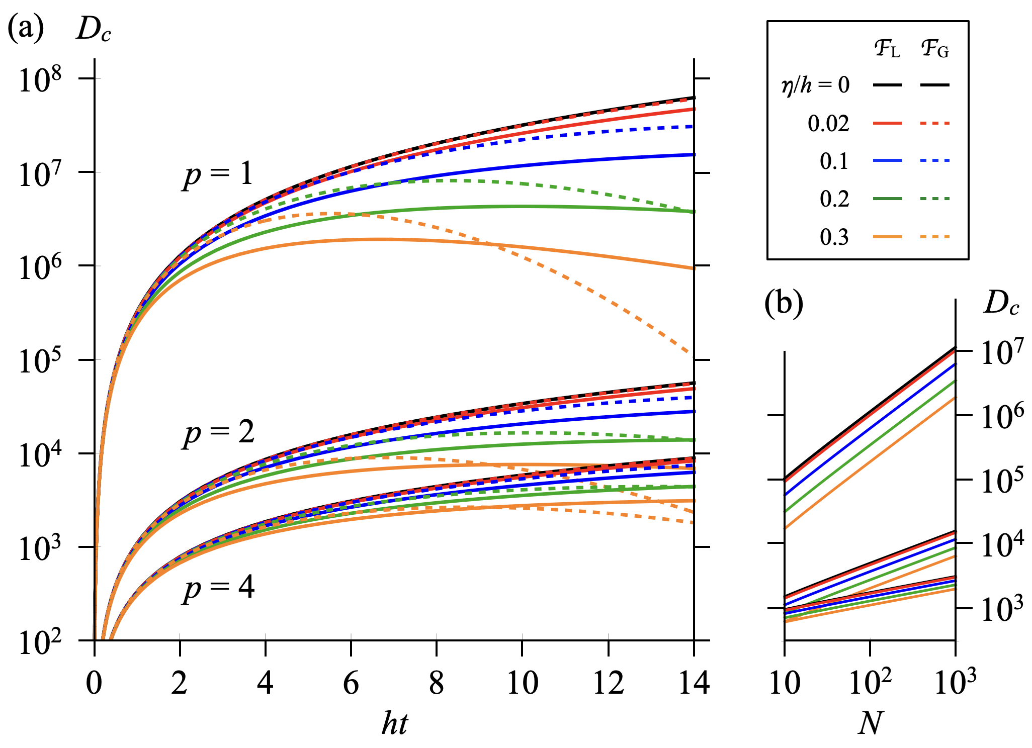
Figure 1: (a) Plot of the upper bound of total circuit depth $D_{c}$ (= Trotter depth cutoff $\times$ gate counts per iteration) versus time for the TFIM ($N=10^{3}$) with different choices for the Trotterization order $p\in\{1,2,4\}$ and the filter $\mathcal{F}\in\{\mathcal{F}_{\rm L},\mathcal{F}_{\rm G}\}$, showing that $\eta$ $(=\sigma\sqrt{2\ln 2})$ exponentially suppresses the bound in a long time. Other parameters are set to $J/h=0.4$, $\varepsilon_{{\rm T},c}=10^{-2}$. The vertical axis is a log scale. (b) Plot of $D_{c}$ versus $N$ for a fixed $ht=6$. Both axes are log scales.

To give an estimate to $M_{c}^{(p)}$, thereby $D_{c}^{(p)}$, we consider the transverse-field Ising model (TFIM) in one dimension:

$$H_{1}=-J\sum_{j=0}^{N-2}\sigma^{z}_{j}\sigma^{z}_{j+1},~{}H_{2}=-h\sum_{j=0}^{N-1}\sigma^{x}_{j},$$ (27)

where $\sigma^{\alpha}$ with $\alpha\in\{x,y,z\}$ are the Pauli matrices, $N$ is the number of spins at sites $j\in[0,N-1]$, $J$ is the Ising coupling, and $h$ is the magnetic field. The TFIM has a paramagnetic ground state (for $J/h<1$) separated from a ferromagnetic state (for $J/h>1$) by a quantum critical point (at $J/h=1$) [39]. Straightforward calculations using Eq. (27) yield the explicit forms of the commutators in Eqs. (23)-(25) and the bounds of the spectral norms. See Appendix A for details.

Figure 1 demonstrates the impact of the filter function on the upper bound of total circuit depth, $D_{c}$, for the TFIM. Here two types of filters $\mathcal{F}_{\rm L}$, $\mathcal{F}_{\rm G}$ are used for comparison. Without filtering ($\eta=0$), the model shows a prohibitive Trotter scaling that appears to prevent QPE simulation on quantum devices. In Fig. 1(a), for spin counts $N=10^{3}$, top black solid curve ($p=1$) exceeds, for example, $D_{c}\sim 10^{7}$ for $ht>6$, which is improved to $D_{c}\sim 10^{4}(10^{3})$ for $p=2(4)$. Figure 1(b) shows that $|D_{c}^{(p)}-D_{c}^{(p^{\prime}\neq p)}|$ is reduced for smaller $N$. In the presence of filtering ($\eta>0$), however, long-time evolution is truncated and $D_{c}$ is significantly improved (colored solid curves for $\mathcal{F}_{\rm L}$; colored dashed curves for $\mathcal{F}_{\rm G}$), thus proposing a route to considerable improvements in QPE-based algorithms. Note that filtering is more effective for smaller $p$ [see Eq. (26)], allowing $D_{c}^{(p)}>D_{c}^{(p^{\prime})}$ for $p<p^{\prime}$ in a long time. Lastly, $D_{c}$ is only a bound. In practice, total circuit depth depends on the choice of $H$, $\mathcal{F}$, and the algorithm.

III Hybrid quantum gap estimation algorithm

III.1 Overview

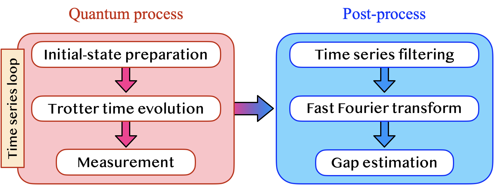
Figure 2: Flowchart for the hybrid QGE algorithm

We now construct a hybrid QGE algorithm and and demonstrate the impact of filtering on time evolution. The algorithm flowchart is depicted in Fig. 2. We start with an input state $|\psi_{\rm I}\rangle$ that overlaps with an exact state $|\psi_{\rm exact}\rangle$ of interest, perform Trotter time evolution, and then readout in the same basis as the input state. The output state oscillates in time at frequencies of the exact energy gaps for any input state satisfying $\langle\psi_{\rm I}|\psi_{\rm exact}\rangle\neq 0$. A classical fast Fourier transform of a time series, after filtered, reveals exact energy gaps within the window $2\eta$ set by the filter. In the following provided are details for quantum process and post-process, respectively.

III.2 Quantum process (online)

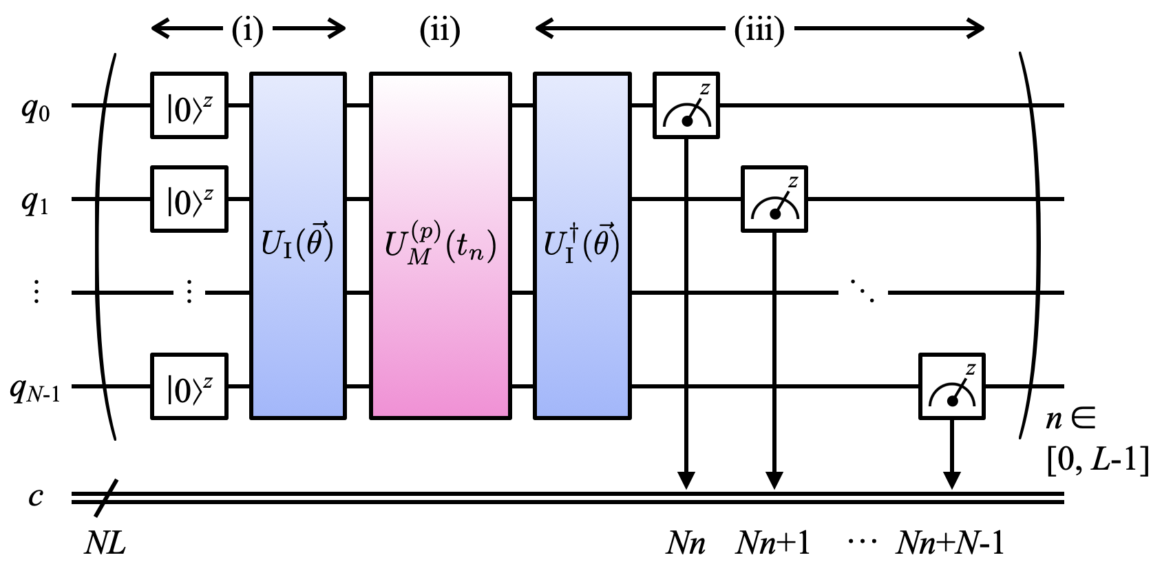
Figure 3: Quantum circuit of the hybrid QGE algorithm for a many-body Hamiltonian $H$. (i) Input preparation: $N$ qubits are prepared (and reset) in the quantum registers, ($q_{0}$, $q_{1}$, $\cdots$, $q_{N-1}$), and rotated by the unitary $U_{\rm I}$ to create the initial state. (ii) Trotter time evolution of the order $p$ by the unitary $U_{M}^{(p)}(t_{n})$. (iii) Measurement: Output qubits are rotated back to compensate $U_{\rm I}$, and $z$-basis (mid-circuit) measurements are carried out to return time-series data (of size $L$) to the classical register, $c$ (while only a single job runs on the quantum processor).

In a quantum processor, each run is iterated over discrete time $t_{n}=n\delta t$ where $n\in[0,L-1]$ for $L$ Fourier sampling points. Figure 3 shows the quantum circuit implementation for our example, the TFIM, in a single run. The circuit proceeds in three steps. First, input qubits are prepared in quantum registers to build the initial state: $|\psi_{\rm I}\rangle=U_{\rm I}\prod_{j=0}^{N-1}|0\rangle_{j}^{z}$. For our purpose, the product-state unitary is a minimal choice (Here entanglement is not essential):

$$U_{\rm I}(\vec{\theta})=\prod_{j=0}^{N-1}R_{j}^{y}(\theta_{j}),$$ (28)

where $R_{j}^{\alpha}(\theta)=\exp(-i\frac{\theta}{2}\sigma_{j}^{\alpha})$, and $\vec{\theta}=(\theta_{0},\theta_{1},\cdots,\theta_{N-1})$ is a free parameter that can be chosen to emphasize different gaps. Second, $|\psi_{\rm I}\rangle$ is time-evolved by applying a sequence of unitaries determined by $H$ and $p\in\{1,2,4\}$:

$$U_{M}^{(1)}(t_{n})=\Big{[}\prod_{j=0}^{N-2}R_{j,j+1}^{zz}\Big{(}\frac{\chi_{n}}{M}\Big{)}R_{j}^{x}\Big{(}\frac{\phi_{n}}{M}\Big{)}\Big{]}^{M},$$

$$U_{M}^{(2)}(t_{n})=\Big{[}\prod_{j=0}^{N-2}R_{j,j+1}^{zz}\Big{(}\frac{\chi_{n}}{2M}\Big{)}R_{j}^{x}\Big{(}\frac{\phi_{n}}{M}\Big{)}R_{j,j+1}^{zz}\Big{(}\frac{\chi_{n}}{2M}\Big{)}\Big{]}^{M},$$

$$U_{M}^{(4)}(t_{n})=\Big{[}\prod_{j=0}^{N-2}R_{j,j+1}^{zz}\Big{(}\frac{\kappa_{4}\chi_{n}}{2M}\Big{)}R_{j}^{x}\Big{(}\frac{\kappa_{4}\phi_{n}}{M}\Big{)}R_{j,j+1}^{zz}\Big{(}\frac{\kappa_{4}\chi_{n}}{M}\Big{)}$$

$$~{}~{}~{}\times R_{j}^{x}\Big{(}\frac{\kappa_{4}\phi_{n}}{M}\Big{)}R_{j,j+1}^{zz}\Big{(}\frac{(1-3\kappa_{4})\chi_{n}}{2M}\Big{)}R_{j}^{x}\Big{(}\frac{(1-4\kappa_{4})\phi_{n}}{M}\Big{)}$$

$$~{}~{}~{}\times R_{j,j+1}^{zz}\Big{(}\frac{(1-3\kappa_{4})\chi_{n}}{2M}\Big{)}R_{j}^{x}\Big{(}\frac{\kappa_{4}\phi_{n}}{M}\Big{)}R_{j,j+1}^{zz}\Big{(}\frac{\kappa_{4}\chi_{n}}{M}\Big{)}$$

$$~{}~{}~{}\times R_{j}^{x}\Big{(}\frac{\kappa_{4}\phi_{n}}{M}\Big{)}R_{j,j+1}^{zz}\Big{(}\frac{\kappa_{4}\chi_{n}}{2M}\Big{)}\Big{]}^{M},$$ (29)

where $R_{j,j+1}^{zz}(\theta)$ $=\exp(-i\frac{\theta}{2}\sigma_{j}^{z}\sigma_{j+1}^{z})$, $\chi_{n}=-2Jt_{n}$, $\phi_{n}=-2ht_{n}$, and $\kappa_{4}=(4-\sqrt[3]{4})^{-1}\approx 0.414$. $M$ repetitions are applied until Trotter error (alternatively, spectral sum or gap estimation error; see Sec. IV.1) is reduced below a tolerance. In the last online step, output qubits are rotated back to the input-state basis and measured. Here, quantum state tomography [40] or ancilla qubits [7, 17] are not involved, thus saving computational resources.

III.3 Post-process (offline)

The time-evolved output state obtained from the quantum circuit is processed offline. In the first offline step, we build time-series data, $\{(t_{n},\mathcal{P}_{n}^{(p)})\}_{n=0}^{L-1}$, where measurement outcomes in the $z$ basis are encoded in:

$$\mathcal{P}_{n}^{(p)}={\rm Tr}[\rho_{0}\rho_{\vec{\theta}}^{(p)}(t_{n})].$$ (30)

Here we define the density matrices $\rho_{0}=$ $\prod_{j=0}^{N-1}|0\rangle_{j}^{z}\langle 0|_{j}^{z}$ for the input registers and $\rho_{\vec{\theta}}^{(p)}(t_{n})=U_{M,\vec{\theta}}^{(p)}(t_{n})\rho_{0}[U_{M,\vec{\theta}}^{(p)}(t_{n})]^{\dagger}$ for the output with the similarity transform $U_{M,\vec{\theta}}^{(p)}(t_{n})=[U_{\rm I}(\vec{\theta})]^{\dagger}$ $U_{M}^{(p)}(t_{n})U_{\rm I}(\vec{\theta})$. Next, Eq. (30) is filtered by $\mathcal{F}_{n}=\mathcal{F}(t_{n})$, and fed into the classical subroutine for a discrete Fourier transform (DFT) which yields a (many-body) spectral function:

$$\mathcal{A}^{(p)}(\omega_{m})=\frac{\delta t}{2\pi}{\rm Re}\sum_{s=\pm}\sum_{n=0}^{L-1}e^{i\omega_{m}t_{sn}}\mathcal{F}_{n}\mathcal{P}_{sn}^{(p)},$$ (31)

where we define discrete frequencies $\omega_{m}=m\delta\omega$, conjugate to $t_{n}$, in units of $\delta t$ and $\delta\omega$ satisfying $\delta\omega\delta t=2\pi/L$, and $m,n\in[0,L-1]$. The $s=+(-)$ terms in Eq. (31) describe causal (anti-causal) processes. In practice, a fast Fourier transform (FFT) is widely adopted to improve computational complexity of the original DFT, $\mathcal{O}(N^{2})$ to $\mathcal{O}(N\log N)$ [41].

To reveal key features of Eq. (31), we consider the continuum limit ($L\rightarrow\infty$):

$$\mathcal{A}^{(p)}(\omega)=\frac{1}{2\pi}\sum_{s=\pm}\int_{-\infty}^{\infty}dt\cos(\omega t)\Theta(st)\mathcal{F}(st)\mathcal{P}^{(p)}(t),$$ (32)

where $\Theta(t)$ is the step function, and $\mathcal{P}^{(p)}(t)={\rm Tr}[\rho_{0}\rho_{\vec{\theta}}^{(p)}(t)]$ $=|\langle\psi_{\rm I}|U_{M}^{(p)}(t)|\psi_{\rm I}\rangle|^{2}\in\mathbb{R}$, that is distinguished from the form $\langle\psi_{\rm I}|U_{M}^{(p)}(t)|\psi_{\rm I}\rangle\in\mathbb{C}$ for eigenvalue estimation [42]. Eq. (32) can be recast further in the convolution form:

$$\mathcal{A}^{(p)}(\omega)=\int_{-\infty}^{\infty}d\tilde{\omega}\tilde{\mathcal{F}}(\tilde{\omega})\mathcal{A}_{0}^{(p)}(\omega-\tilde{\omega}),$$ (33)

where $\tilde{\mathcal{F}}$ represents the filter in Fourier space:

$$\tilde{\mathcal{F}}(\omega)=\frac{1}{\pi}\int_{0}^{\infty}dt\cos(\omega t)\mathcal{F}(t),$$ (34)

and $\mathcal{A}_{0}^{(p)}(\omega)\equiv\mathcal{A}^{(p)}(\omega)|_{\mathcal{F}=1}$ (without filtering). Two features of Eq. (33) are addressed below.

First, peak centers in $\mathcal{A}_{0}^{(p)}$ return exact energy gaps for any choices of $H$ and $|\psi_{\rm I}\rangle$. To show this, ignoring Trotter error for $M>M_{c}$, we approximate $U_{M}^{(p)}(t)\approx e^{-iHt}$. We then expand $|\psi_{\rm I}\rangle=\sum_{u}c_{u}|u\rangle$, where eigenstates $|u\rangle$ satisfy $H|u\rangle=\mathcal{E}_{u}|u\rangle$ with eigenenergies $\mathcal{E}_{u}$, and plug it in $\mathcal{A}_{0}^{(p)}$ to derive the spectral representation (Hereafter, we drop the superscript, $p$):

$$\mathcal{A}_{0}(\omega)=\sum_{u,v}|c_{u}|^{2}|c_{v}|^{2}\delta(\omega-\Delta_{u,v}),$$ (35)

where we define the Dirac delta function $\delta(\omega)=\frac{1}{2\pi}\int dte^{i\omega t}$ and exact energy gaps $\Delta_{u,v}=\mathcal{E}_{u}-\mathcal{E}_{v}$. For estimation of a target, say, $\Delta_{u,v}$, the condition of $|c_{u}||c_{v}|\neq 0$ is generally demanded. Without loss of generality, we can drop the redundant sum over $u\leq v$ to focus on the partial sum over $u>v$.

Second, Eq. (33) converts delta functions in Eq. (35) into the line shapes set by Eq. (34):

$$\mathcal{A}(\omega)=\sum_{u,v}|c_{u}|^{2}|c_{v}|^{2}\tilde{\mathcal{F}}(\omega-\Delta_{u,v}).$$ (36)

For the choice of $\mathcal{F}_{\rm L}(t)=e^{-\eta t}$, $\tilde{\mathcal{F}}(\omega)$ describes a Lorentzian line shape: $\tilde{\mathcal{F}}_{\rm L}(\omega)=\frac{1}{\pi}\frac{\eta}{\omega^{2}+\eta^{2}}$. For $\mathcal{F}_{\rm G}(t)=e^{-\sigma^{2}t^{2}/2}$, it turns out to be a Gaussian line shape: $\tilde{\mathcal{F}}_{\rm G}(\omega)=\frac{1}{\sqrt{2\pi}\sigma}e^{-\frac{\omega^{2}}{2\sigma^{2}}}$. Here, the broadening $2\eta$ defines the full width at half maximum of the line shape, and has a connection to $\sigma$: $\eta=\sigma\sqrt{2\ln 2}$. It has an operating range designed to maximize simulation performance: $2\eta$ is bounded below by Trotter error $\varepsilon_{\rm T}$ and above by peak-to-peak separations to hold spectral resolutions in gap estimation. See Sec. IV.2 for further discussion.

The last offline step establishes a consistent gap estimation protocol for Eq. (31). We need to start with an initial guess of the energy gap, $\Delta_{0}$, e.g., mean-field or perturbative. Here we use perturbation theory for the TFIM with open boundaries: $\Delta_{0}/h=2[1-(1-1/N)J/h]$ (See Appendix B). (We focus on the lowest gap but can find any gap by adjusting the initial guess.) We then search for the peak center in the range $\Delta_{0}-\delta\Delta/2\leq\omega\leq\Delta_{0}+\delta\Delta/2$ to find the unbiased estimate of $\Delta$. Here the search window $\delta\Delta$ is initially set to $2\eta$. If $\Delta$ is not within the range, we restart with either a new choice of $\delta\Delta$ or $\Delta_{0}$. This process is iterated until a solution is found.

IV Results

So far, we have proposed the hybrid QGE algorithm using a filtered time series, thereby requiring shallow circuits. In this section, we demonstrate proof-of-concept simulation results using the TFIM of the small size $N\in\{2,3,4,5\}$ as a benchmark model [43]. The results are compared between different choices of filter $\mathcal{F}$ and Trotterization order $p$. Here the study on noise-induced error in quantum processes is beyond our scope. To demonstrate the algorithm, we discuss our implementation case: gaps of the TFIM and the gap-based paramagnetic phase diagram determined by finite-size extrapolation.

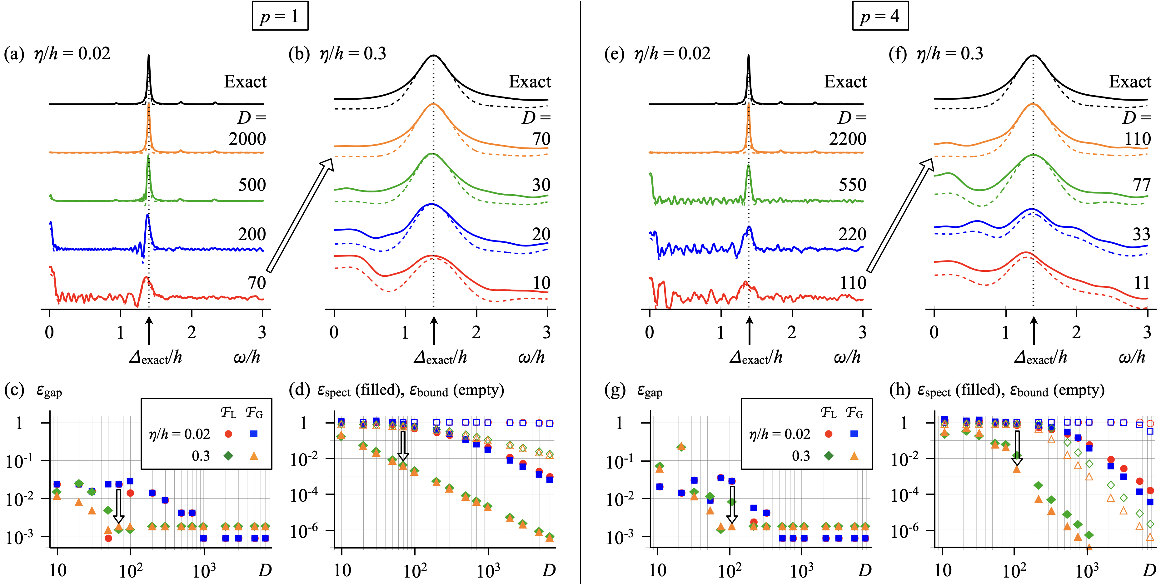
Figure 4: Simulation results demonstrating convergence boost of QGE by filtering. The results are compared between different choices of the Trotterization order $p=$ (a-d) 1, (e-h) 4, the broadening $\eta/h=$ (a,e) 0.02, (b,f) 0.3, and the filter $\mathcal{F}\in\{\mathcal{F}_{\rm L},\mathcal{F}_{\rm G}\}$. The top panels show the spectral function $\mathcal{A}$ versus frequency $\omega$ for the TFIM of $N=4$, $J/h=0.4$. Colored solid (dashed) curves are the results for $\mathcal{F}=\mathcal{F}_{\rm L}$ ($\mathcal{F}_{\rm G}$). All cases show convergence to the exact form (top black curve) for increasing circuit depth $D$. The upper bound of $D$ is effectively reduced by increasing $\eta$. Black vertical dotted line refers to the exact gap $\Delta_{\rm exact}$. Tilted black empty arrow shows how $\mathcal{A}$ evolves as $\eta$ increases for $D=$ (a,b) 70, (e,f) 110. The bottom panels indicate (c,g) gap estimate error $\varepsilon_{\rm gap}$ and (d,h) spectral lineshape error $\varepsilon_{\rm spect}$ (filled symbols), bounded above by $\varepsilon_{\rm bound}$ (empty symbols), as a function of $D$ for different choices of $\mathcal{F}$, $\eta$. In all simulations, 1024 measurement shots were used, and other parameters are: $\theta_{j}=0.27\pi$ (uniform input orientations over sites), $\delta\omega=\eta/4$, $L=2\lceil 7/\delta\omega\rceil$, where $\lceil x\rceil$ is the ceiling function of $x$.

IV.1 Convergence boost of QGE by filtering

The central assertion in Sec. II was that filtering Trotter time evolution for long times effectively lowers the upper bound of circuit depth for a fixed Trotter truncation error. Here we numerically confirm that the filtering method can be leveraged to boost the convergence of the hybrid QGE algorithm.

Figure 4 shows simulation results for $N=4$, $J/h=0.4$ but with different choices of $p\in\{1,4\}$, $\mathcal{F}\in\{\mathcal{F}_{\rm L},\mathcal{F}_{\rm G}\}$. Input orientations are fixed here, but, later on, will be tuned for further investigation. The top panels indicate that increasing $\eta$ gives better convergence of $\mathcal{A}$ to the exact form with $D$. The plots with $D\ll\tilde{D}_{c}$, where $\tilde{D}_{c}$ is the empirical bound of circuit depth, are featured by satellite peaks (apart from the main peak) which are governed by the Floquet stroboscopic dynamics [44]. If the satellite peaks are separated within the resolution limit $2\eta$, they are smoothed out, thereby leaving only the main peak behind. Black empty arrow highlights $D=70$ $(110)$ for $p=1(4)$, allowing direct comparison between the plots with various $\eta$ but fixed $D$.

Either choice of $p$ or $\mathcal{F}$ can change the characteristics of convergence while overall trends hold. To show this clearly, we measure different types of errors from the data and compare them. First off, we define the gap estimate error:

$$\varepsilon_{\rm gap}=|\Delta-\Delta_{\rm exact}|/\Delta_{\rm exact},$$ (37)

where $\Delta$ is a gap estimate obtained using the protocol outlined in Sec. III.3, and $\Delta_{\rm exact}$ is the exact gap as a reference for a small-size system. Figure 4(c),(g) show the evolution of $\varepsilon_{\rm gap}$ with $D$. For each choice of ($\mathcal{F}$, $\eta$), we can estimate the circuit depth cutoff $\tilde{D}_{c}$ where $\varepsilon_{\rm gap}$ reaches the lower bound. Plateaus arise since the frequency resolution is limited by $2\eta$. We find that $\tilde{D}_{c}$ is lowered for larger $\eta$ with an extra shift relying on the choice of $\mathcal{F}$. For $\eta/h=0.3$, the shift is visible: $\tilde{D}_{c,{\rm G}}<\tilde{D}_{c,{\rm L}}$. Such a distinction is because the Gaussian line shape is more concentrated at the center than the Lorentzian case, efficiently suppressing interference with nearby peaks. The distinction is, however, negligible for $\eta/h=0.02$. Meanwhile, the effect of higher $p$ is not as impressive as we might expect. Comparing the data for $p=4$ with $p=1$, for example, $\tilde{D}_{c}$ is slightly lowered (lifted) for $\eta/h=0.02(0.3)$. In fact, this is nothing but what Fig. 1 implies: For $\eta\rightarrow 0$, $p=4$ outperforms $p=1$ in the entire time domain, while it does not for large $\eta$ since $p=1$ is improved more than $p=4$ at long times.

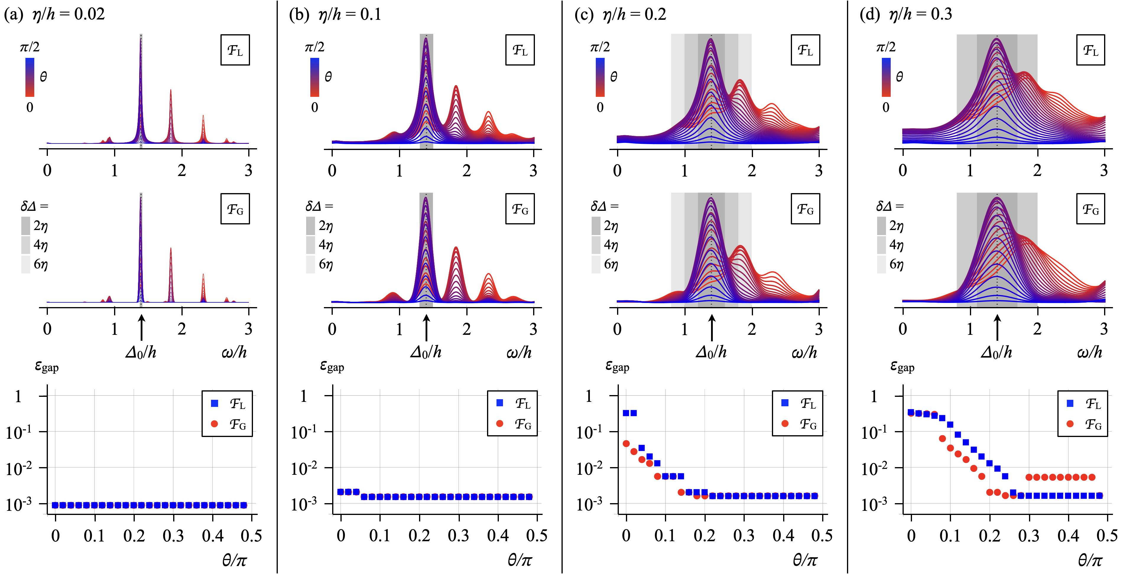
Figure 5: Simulation results demonstrating the operating range of filtering. The results are compared between different choices of the broadening $\eta/h=$ (a) 0.02, (b) 0.1, (c) 0.2, (d) 0.3, the filter $\mathcal{F}\in\{\mathcal{F}_{\rm L},\mathcal{F}_{\rm G}\}$, but with Trotterization set to the order $p=1$. The top and middle panels show the spectral function $\mathcal{A}$ versus frequency $\omega$ for the TFIM of $N=4$, $J/h=0.4$ but with different $\mathcal{F}$. Here circuit depth is set to $D=$ (a) 2000, (b) 300, (c) 100, (d) 70 (satisfying the spectral lineshape error $\varepsilon_{\rm spect}<10^{-2}$), and $\mathcal{A}$’s are sampled with uniformly selected input orientations $\theta_{l}/\pi=l/50$, $l\in[0,24]$ (but irrespective of sites). For each $\theta_{l}$, starting with the initial guess for energy gap $\Delta_{0}$ (black vertical dotted line), we search for the peak center close to $\Delta_{0}$ within the window $[\Delta_{0}-\delta\Delta/2,\Delta_{0}+\delta\Delta/2]$ by progressively increasing $\delta\Delta$ (gray shades). The bottom panels show the gap estimate error $\varepsilon_{\rm gap}$ as a function of $\theta$ for both $\mathcal{F}_{\rm L},\mathcal{F}_{\rm G}$. Other parameters are the same as Fig. 4.

Another useful measure is the spectral lineshape error (as a square root of the measure known as the coefficient of determination in statistics [45]):

$$\varepsilon_{\rm spect}=\sqrt{\frac{\sum_{m=0}^{L-1}[\mathcal{A}(\omega_{m})-\mathcal{A}_{\rm exact}(\omega_{m})]^{2}}{\sum_{m=0}^{L-1}[\mathcal{A}(\omega_{m})-\mathcal{A}_{\rm av}]^{2}}},$$ (38)

where $\mathcal{A}_{\rm av}=\frac{1}{L}\sum_{m=0}^{L-1}\mathcal{A}(\omega_{m})$. Since Eq. (37) only measures error in the main peak center, error may be accidentally reduced when satellite peaks dwell around the main peak for small $D$. Eq. (38), by contrast, accumulates errors in the spectral line shape over the entire frequency domain, and therefore provides a more consistent measure. Figures 4(d),(h) show the counterpart to Figs. 4(c),(g) for different choices of $(p,\mathcal{F},\eta)$. The overall trend of $\varepsilon_{\rm spect}$ is matched with $\varepsilon_{\rm gap}$, but without plateaus since the resolution of $\varepsilon_{\rm spect}$ is not affected by $\eta$.

Lastly, it is useful to derive the upper bound of Eq. (38). A starting point is the Trotter truncation error $||\mathcal{F}(t_{n})[\rho_{M}(t_{n})-\rho_{\rm exact}(t_{n})]||$ with the upper bound [Eq. (22)]. Since the spectral norm $||\cdot||$ plays a key role in deriving the upper bound, we define $\hat{\mathcal{A}}(\omega_{m})$ by replacing ${\rm Tr}[\cdot]$ in Eq. (31) by $||\cdot||$. Then the upper bound of Eq. (38) has the form:

$$\varepsilon_{\rm bound}=\sqrt{\frac{\sum_{m=0}^{L-1}[\hat{\mathcal{A}}(\omega_{m})-\hat{\mathcal{A}}_{\rm exact}(\omega_{m})]^{2}}{\sum_{m=0}^{L-1}[\hat{\mathcal{A}}(\omega_{m})-\hat{\mathcal{A}}_{\rm av}]^{2}}},$$ (39)

where $\hat{\mathcal{A}}(\omega_{m})=\hat{\mathcal{A}}_{\rm exact}(\omega_{m})+\delta\hat{\mathcal{A}}(\omega_{m})$, with

$$\left\{\begin{array}[]{c}\hat{\mathcal{A}}_{\rm exact}\\ \delta\hat{\mathcal{A}}\end{array}\right\}=\frac{\delta t}{2\pi}{\rm Re}\sum_{s=\pm}\sum_{n=0}^{L-1}e^{i\omega_{m}t_{sn}}\mathcal{F}_{n}\left\{\begin{array}[]{c}1\\ C^{(p)}t_{sn}^{p+1}/M^{p}\end{array}\right\},$$ (40)

and $\hat{\mathcal{A}}_{\rm av}=\frac{1}{L}\sum_{m=0}^{L-1}\hat{\mathcal{A}}(\omega_{m})$. Empty symbols in Fig. 4(d),(h) represent Eq. (39), revealing a similar trend to filled symbols but with overestimation in all range of circuit depth.

IV.2 Operating range of filtering

We just showed that the filtering method can be leveraged to improve the convergence of the hybrid QGE algorithm but only with the input unitary $U_{\rm I}(\vec{\theta})$ fixed to a certain form. In fact, $U_{\rm I}(\vec{\theta})$ provides a control knob that allows further investigation of our algorithm. Importantly, the filter has an operating range designed to maximize simulation performance. Specifically, $\eta$ in the filter is bounded above by spectral resolution set by the algorithm and model. Tuning $\vec{\theta}$ in $U_{\rm I}(\vec{\theta})$ can impact the resolution by changing relative peak heights. Here we map out the spectral functions with different ratios of peak heights for different choices of $\vec{\theta}$ to numerically confirm the upper bound of $\eta$.

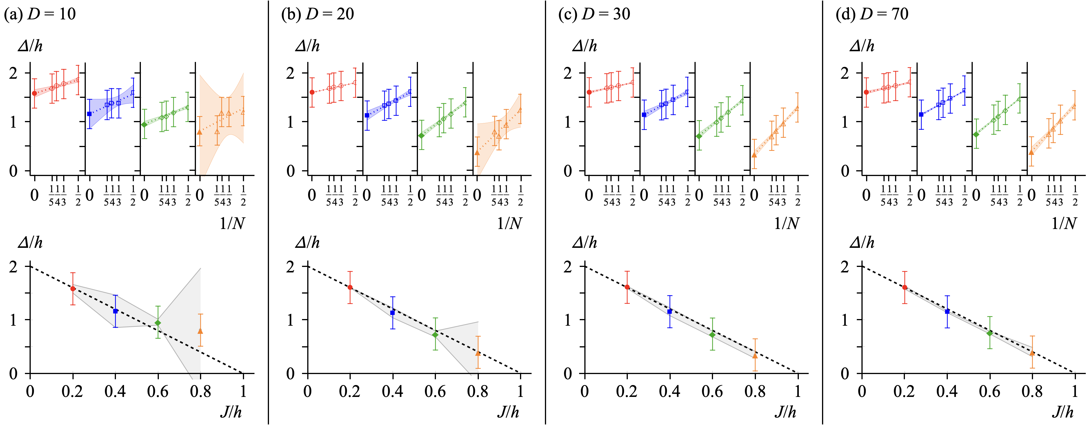
Figure 6: Stages of construction for the gap-based phase diagram of quantum paramagnet. In the hybrid QGE simulation, we fix the Trotterization order $p=1$, the filter $\mathcal{F}=\mathcal{F}_{\rm L}$, and the broadening $\eta/h=0.3$. Each column shows progress on convergence for increasing circuit depth $D=$ (a) 10, (b) 20, (c) 30, (d) 70. The top panels show finite-size scaling of energy gap for the TFIM. Empty symbols indicate the samples of gap estimates $\{\Delta_{N,J/h}\}$ for $N=2-5$, $J/h=$ 0.2 (red), 0.4 (blue), 0.6 (green), 0.8 (orange). Vertical fence symbols set error bounds $[\Delta-\eta,\Delta+\eta]$ around $\Delta$. Filled symbols are extrapolation to $N\rightarrow\infty$ by linear regression (dotted lines). Colored shades are confidence bands with a 95% confidence level. The bottom panels show the gap-based phase diagram of quantum paramagnet ($J<h$). Filled symbols are the extrapolated data points at $N\rightarrow\infty$ (obtained from the top panels). Gray shades are interpolation of the confidence band edges (at $N\rightarrow\infty$) for different $J/h$. Black dashed line indicates the exact gap $\Delta_{\rm exact}^{(N\rightarrow\infty)}$. Other parameters are the same as Fig. 4.

Figure 5 shows simulation results for $N=4$, $J/h=0.4$ but with different choices of $\eta/h\in\{0.02,0.1,0.2,0.3\}$. Here we use $p=1$ Trotterization. The top and middle panels, assuming $\theta_{j}=\theta$, i.e., uniform input orientation over sites $j$, indicates that tuning $\theta\in[0,\pi/2]$ emphasizes different peaks in $\mathcal{A}$ for the choice of $\mathcal{F}_{\rm L}$ (top), $\mathcal{F}_{\rm G}$ (middle). The gap is estimated starting with an initial guess $\Delta_{0}$ (indicated by arrow) and progressively increasing the search window $\delta\Delta$ (gray shades). The bottom panel shows the gap estimate error $\varepsilon_{\rm gap}$ as a function of $\theta$. According to Eq. (35), a gap estimate without filtering is invariant under any choice of $\theta$. This is exemplified by Fig. 5(a), where $2\eta$ is far below peak-to-peak resolution, and thus $\varepsilon_{\rm gap}$ is constant over $\theta$. Meanwhile, filtering makes each peak broadened by $2\eta$ [see Eq. (36)], thus allowing the overlap between neighbor peaks. The tail of neighbor peaks generally forms a slanted background that shifts the peak center in our interest. Figure 5(b-d), in contrast to Fig. 5(a), reveals a non-uniform modification to $\varepsilon_{\rm gap}$ over $\theta$, growing for increasing $\eta$. Specifically, for $\theta$ close to $\pi/2$, $\varepsilon_{\rm gap}$ remains minimal, since the neighbor peak centered at $\omega/h\approx 1.845$ is not well developed. As we tune $\theta$ away from $\pi/2$, however, the neighbor peak grows and eventually dominates the main peak. For larger $\eta$, a minor peak is buried more easily under the background, thus shifting the peak center from one to another and lifting $\varepsilon_{\rm gap}$. The choice of $\mathcal{F}$ also affects the above argument since it sets the background in a different form. In Fig. 5(d), for example, $\mathcal{F}_{\rm G}$ lowers $\varepsilon_{\rm gap}$ more than $\mathcal{F}_{\rm L}$ for $\theta\leq 0.25\pi$, while it is reversed for $0.3\pi\leq\theta\leq 0.46\pi$. As mentioned before, this is attributed to the fact that the Gaussian line shape is more concentrated at the center than the Lorentzian case. Appendix C describes a toy model to support our argument on peak center shift.

IV.3 Finite-size scaling of quantum paramagnetic gap

Previously, we demonstrated the performance of the hybrid QGE algorithm using shallow quantum circuits in the filtering method, and discussed its validity. Our algorithm can be combined with post-processes to calculate important physical quantities such as a (gap-based) phase diagram. As a benchmark, we construct the phase diagram of quantum paramagnet ($J<h$), and compare the simulation result with the exact solution. Here we focus on the case with $p=1$, $\mathcal{F}=\mathcal{F}_{\rm L}$, and $\eta/h=0.3$.

Construction is organized into three stages. First, from the simulation, we obtain the sample of gap estimates $\{\Delta_{N,J/h}\}$ for $N\in\{2,3,4,5\}$, $J/h\in\{0.2,0.4,0.6,0.8\}$. If the broadening $\eta$ is comparable to spectral resolution [See Fig. 5(c,d)], we need a protocol for addressing the range of $\theta$ where $\varepsilon_{\rm gap}$ is minimized. It turns out that a sufficient condition is to maximize the height of a target peak. Empty symbols in the top panels of Fig. 6 indicate data sampled in the above manner. Next, for each choice of $J/h$, we use linear regression to extrapolate the data for $N\in\{2,3,4,5\}$ to $N\rightarrow\infty$ (filled symbols). The result is accompanied by confidence bands (colored shades) that represent misalignment of data points. In the last stage, the extrapolated data is rearranged to construct the phase diagram of quantum paramagnet. The bottom panels in Fig. 6 show the results. Here the black dashed lines compare with the exact gap $\Delta_{\rm exact}^{(N\rightarrow\infty)}=2|h-J|$ (See Appendix B for derivation).

Finally, we confirm convergence of the phase diagram for increasing circuit depth $D$. The columns in Fig. 6 are arranged in the ascending order of $D$ [in the same way as Fig. 4(b)]. For small $D$, $\Delta$ is off from $\Delta_{\rm exact}$ and confidence bands are comparable to/exceed error bounds $2\eta$ (depending on the choice of $J/h$), while, for increasing $D$, they are safely getting inside $2\eta$ and eventually converge to $\Delta_{\rm exact}$.

V Conclusion

We developed a hybrid QGE algorithm using a filtered time series. We found, using the filter, exponential improvement of circuit depth at long times, and mapped out the role of various input states to reveal the operating range of filtering. We finally showed how our protocol can be used. We constructed the gap-based paramagnetic phase diagram for a minimal spin model, which demonstrates how a quantum device can offer memory advantage in finite-size extrapolation of energy gaps.

Further improvements by, e.g., Cartan decomposition [46] and Bayesian methods [47, 16, 17], could allow applications to many-body models requiring more gates to implement time evolution. Our approach can also be applied to hybrid DMFT algorithms [31, 32, 33], where speedup and noise resilience were recently observed [33], and a recent proposal of measurement-based hybrid algorithm for eigenvalue estimation [48].

Appendix A Explicit forms of Eqs. (23)-(25) for the TFIM

Here, using Eq. (27) for the TFIM, we explicitly calculate the spectral norms in Eqs. (23)-(25). The commutators of $H_{1}$ and $H_{2}$ of interest can be successively derived as follows:

$$[H_{1},H_{2}]=2iJh\sum_{j=0}^{N-2}(\sigma^{y}_{j}\sigma^{z}_{j+1}+\sigma^{z}_{j}\sigma^{y}_{j+1}),$$ (41)

$$[H_{1},[H_{1},H_{2}]]=-8J^{2}h\bigg{[}\sum_{j=0}^{N-1}\sigma^{x}_{j}+\sum_{j=0}^{N-3}\sigma^{z}_{j}\sigma^{x}_{j+1}\sigma^{z}_{j+2}\bigg{]},$$ (42)

$$[H_{2},[H_{1},H_{2}]]=-8Jh^{2}\sum_{j=0}^{N-2}(\sigma^{y}_{j}\sigma^{y}_{j+1}-\sigma^{z}_{j}\sigma^{z}_{j+1}),$$ (43)

$$[H_{1},[H_{1},[H_{2},[H_{1},H_{2}]]]]=[H_{1},[H_{2},[H_{1},[H_{1},H_{2}]]]]$$

$$=-64J^{3}h^{2}\bigg{[}\sum_{j=0}^{N-2}\sigma^{y}_{j}\sigma^{y}_{j+1}-\sum_{j=0}^{N-4}\sigma^{z}_{j}\sigma^{x}_{j+1}\sigma^{x}_{j+2}\sigma^{z}_{j+3}\bigg{]},$$ (44)

$$[H_{2},[H_{1},[H_{2},[H_{1},H_{2}]]]]=[H_{2},[H_{2},[H_{1},[H_{1},H_{2}]]]]$$

$$=64J^{2}h^{3}\sum_{j=0}^{N-3}(\sigma^{y}_{j}\sigma^{x}_{j+1}\sigma^{y}_{j+2}-\sigma^{z}_{j}\sigma^{x}_{j+1}\sigma^{z}_{j+2}).$$ (45)

All others are connected with Eqs. (42) and (43):

$$[H_{\gamma},[H_{1},[H_{1},[H_{1},H_{2}]]]]=8J^{2}[H_{\gamma},[H_{1},H_{2}]],$$ (46)

$$[H_{\gamma},[H_{2},[H_{2},[H_{1},H_{2}]]]]=16h^{2}[H_{\gamma},[H_{1},H_{2}]],$$ (47)

where $\gamma\in\{1,2\}$. In the above derivation, we used the identities: $[AB,C]=A[B,C]$ $+[A,C]B$ for the matrices $A$, $B$, $C$, $[\sigma^{\alpha},\sigma^{\beta}]=2i\varepsilon_{\alpha\beta\gamma}\sigma^{\gamma}$, $\{\sigma^{\alpha},\sigma^{\beta}\}=2\delta_{\alpha\beta}I$ with the Kronecker delta $\delta_{\alpha\beta}$, the Levi-Civita symbol $\varepsilon_{\alpha\beta\gamma}$, and $\alpha,\beta,\gamma\in\{x,y,z\}$. For the spectral norms of Eqs. (41)-(47), we apply the properties: $||cA||=|c|||A||$, $||AB||\leq||A||~{}||B||$, $||A+B||\leq||A||+||B||$, and $||e^{iA}||=1$ if $A=A^{\dagger}$, where $A$, $B$ are matrices, and $c$ is a scalar. It turns out that the upper bounds of the commutators are summarized:

$$||[\tilde{H}_{1},\tilde{H}_{2}]|| \leq 4(N-1),$$ (48)

$$||[\tilde{H}_{\gamma},[\tilde{H}_{1},\tilde{H}_{2}]]|| \leq 16(N-1),$$ (49)

$$||[\tilde{H}_{\gamma},[\tilde{H}_{\lambda},[\tilde{H}_{\bar{\lambda}},[\tilde{H}_{1},\tilde{H}_{2}]]]]|| \leq 128(N-2),$$ (50)

$$||[\tilde{H}_{\gamma},[\tilde{H}_{\lambda},[\tilde{H}_{\lambda},[\tilde{H}_{1},\tilde{H}_{2}]]]]|| \leq 128\lambda(N-1),$$ (51)

where $\tilde{H}_{1}=H_{1}/|J|$, $\tilde{H}_{2}=H_{2}/|h|$, $\gamma,\lambda\in\{1,2\}$, and $\bar{\lambda}=1(2)$ if $\lambda=2(1)$. Eqs. (48)-(51) allows deriving the upper bounds of Eqs. (23)-(25), thereby Eq. (22).

Appendix B Reference formulas for energy gap of the TFIM

Here we derive the reference formulas for energy gap of the TFIM using (i) perturbation theory, (ii) exact methods.

B.1 Initial guess of energy gap

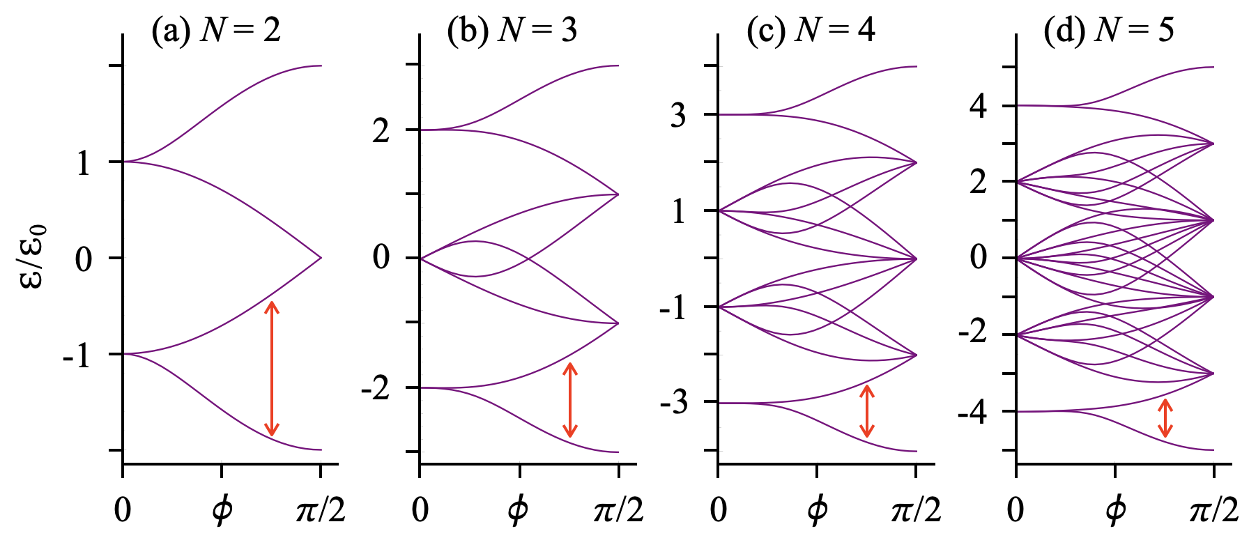
Figure 7: Energy spectrum of the TFIM for $N=2-5$ as a function of $\phi[=\cot^{-1}(J/h)]$. Here we have ferromagnet (or paramagnet) at $\phi=0$ (or $\pi/2$), and red arrow indicates the lowest energy gap of quantum paramagnet ($\pi/4<\phi\leq\pi/2$).

Figure 7 shows the energy spectrum of the TFIM for $N=2-5$, where the lowest energy gap of interest is indicated by the red arrow. In the hybrid QGE algorithm, gap estimation generally requires an initial guess of the energy gap. For this purpose, we consider a generally applicable procedure: perturbation expansion [39]. In our case, we perturb in powers of $J/h$ to find the approximate energy gap of the quantum paramagnet. For the TFIM with $N$ spins, a spin-flip from the paramagnetic ground state $\prod_{j=1}^{N}|0\rangle_{j}^{z}$ requires excitation energy $2h-2J$ for $N-2$ bulk spins and $2h-J$ for two boundary spins. Averaging excitation energies over all spins yields an approximate formula for energy gap:

$$\Delta_{0}/h =[(N-2)(2h-2J)+2(2h-J)]/(Nh)$$

$$=2[1-(1-1/N)J/h],$$ (52)

that is reduced to the case with periodic boundaries [39]:

$$\Delta_{0}/h|_{N\rightarrow\infty}=2(1-J/h).$$ (53)

This expression for $\Delta_{0}$ shows how we derived the initial guess for the gap and also establishes that perturbative methods can, in other models, be used to define the guess.

B.2 Exact energy gap

The TFIM is tractable in the limit $N\rightarrow\infty$. An exact solution provides a reference to compare with the simulation result. Using the Jordan-Wigner transformation [49]: $\sigma_{j}^{x}=1-$ $2c_{j}^{\dagger}c_{j}$, $\sigma_{j}^{z}=-\prod_{k<j}(1-2c_{k}^{\dagger}c_{k})(c_{j}+c_{j}^{\dagger})$, the TFIM is mapped to the Kitaev model describing p-wave superconductor:

$$H_{\rm K}=-w\sum_{j=1}^{N-1}(c_{j}^{\dagger}c_{j+1}+c_{j}^{\dagger}c_{j+1}^{\dagger}+{\rm H.c.})-\mu\sum_{j=1}^{N}\delta n_{j},$$ (54)

where $w(=J)$ is the hopping/pairing energy, $\mu(=-2h)$ is the chemical potential, and $\delta n_{j}=c_{j}^{\dagger}c_{j}^{\vphantom{\dagger}}$ $-1/2$. Assuming periodic boundaries, $H_{\rm K}$ can be diagonalized by the Bogoliubov transformation [39]. The result yields the exact form of the upper and lower energy bands:

$$\mathcal{E}_{\bf k}^{\pm}=\pm\sqrt{J^{2}+h^{2}-2Jh\cos(ka)},$$ (55)

where $k$ is momentum, and $a$ is the lattice constant. The lowest energy gap between two bands is therefore given by the energy difference at ${\bf k}=0$:

$$\Delta_{\rm exact}^{(N\rightarrow\infty)}=\mathcal{E}_{{\bf k}=0}^{+}-\mathcal{E}_{{\bf k}=0}^{-}=2|h-J|,$$ (56)

consistent with Eq. (53) in the paramagnetic regime ($J<h$).

Appendix C Toy model for peak center shift

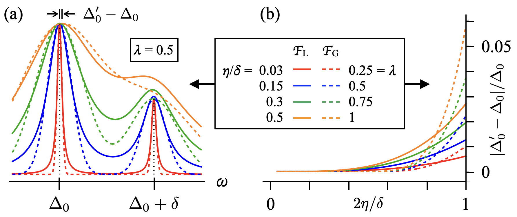
Figure 8: (a) Spectral function for two peaks separated by $\delta/\Delta_{0}=0.6$ with different choices of the broadening $\eta$ but fixed relative height $\lambda=0.5$. Here all plots are normalized and the vertical black dotted lines indicate the reference to the peak centers at $\omega=\Delta_{0},\Delta_{0}+\delta$ for $\eta\rightarrow 0$. (b) Peak center shift $|\Delta^{\prime}_{0}-\Delta_{0}|/\Delta_{0}$ as a function of $\eta$ for different choices of $\lambda$ and the filter $\mathcal{F}\in\{\mathcal{F}_{\rm L},\mathcal{F}_{\rm G}\}$.

Here we describe a toy model for peak center shift to support the argument in Sec. IV.2. In general, peak centers are subject to shift when the separation between peaks is comparable to the broadening of each peak. To show this, we model the spectral function for two peaks separated by $\delta$:

$$\mathcal{A}(\omega)\propto\mathcal{A}_{0}(\omega-\Delta_{0})+\lambda\mathcal{A}_{0}(\omega-\Delta_{0}-\delta),$$ (57)

where we set

$$\mathcal{A}_{0}(\omega)=\left\{\begin{array}[]{cc}\frac{1}{\pi}\frac{\eta}{\omega^{2}+\eta^{2}},&\textrm{Lorentzian}\\ \frac{1}{\sqrt{2\pi}\sigma}e^{-\frac{\omega^{2}}{2\sigma^{2}}},&\textrm{Gaussian}\end{array}\right.$$ (60)

describing an isolated Lorentzian (Gaussian) peak associated with the filter $\mathcal{F}_{\rm L(G)}$, $\eta=\sigma\sqrt{2\ln 2}$, and $\lambda$ controls the second peak height. Figure 8(a) shows how much the original line shape is modified when two peaks are overlapped in the tail for different choices of $\eta$ but fixed $\lambda$. In Fig. 8(b), we focus on the first peak at $\omega=\Delta_{0}$ and measure the peak center shift $|\Delta^{\prime}_{0}-\Delta_{0}|/\Delta_{0}$ as a function of $\eta$ for different choices of $\lambda$. The result implies: (i) the peak center shift is enhanced for increasing $\eta$, (ii) it is enhanced (suppressed) for increasing (decreasing) symmetry between peaks, (iii) $\mathcal{F}_{\rm L(G)}$ induces larger shift than $\mathcal{F}_{\rm G(L)}$ for $2\eta/\delta\lesssim(\gtrsim)$ 0.85.

References

- Feynman [1982] R. P. Feynman, Simulating physics with computers, Int. J. Theor. Phys. 21, 467 (1982).
- Lloyd [1996] S. Lloyd, Universal quantum simulators, Science 273, 1073 (1996).
- Abrams and Lloyd [1999] D. S. Abrams and S. Lloyd, Quantum Algorithm Providing Exponential Speed Increase for Finding Eigenvalues and Eigenvectors, Phys. Rev. Lett. 83, 5162 (1999).
- Nielsen and Chuang [2010] M. A. Nielsen and I. L. Chuang, Quantum Computation and Quantum Information (Cambridge University Press, 2010).
- Yung et al. [2014] M.-H. Yung, J. D. Whitfield, S. Boixo, D. G. Tempel, and A. Aspuru-Guzik, Introduction to Quantum Algorithms for Physics and Chemistry, in Quantum Information and Computation for Chemistry (John Wiley & Sons, Ltd, 2014) Chap. 3, pp. 67–106.
- Kitaev [1996] A. Kitaev, Quantum measurements and the Abelian stabilizer problem, Electr. Coll. Comput. Complex. TR96-003 (1996).
- Somma et al. [2002] R. Somma, G. Ortiz, J. E. Gubernatis, E. Knill, and R. Laflamme, Simulating physical phenomena by quantum networks, Phys. Rev. A 65, 042323 (2002).
- Somma [2019] R. D. Somma, Quantum eigenvalue estimation via time series analysis, New J. Phys. 21, 123025 (2019).
- O’Brien et al. [2019] T. E. O’Brien, B. Tarasinski, and B. M. Terhal, Quantum phase estimation of multiple eigenvalues for small-scale (noisy) experiments, New J. Phys. 21, 023022 (2019).
- O’Brien et al. [2021] T. E. O’Brien, S. Polla, N. C. Rubin, W. J. Huggins, S. McArdle, S. Boixo, J. R. McClean, and R. Babbush, Error Mitigation via Verified Phase Estimation, PRX Quantum 2, 020317 (2021).
- Lin and Tong [2022] L. Lin and Y. Tong, Heisenberg-Limited Ground-State Energy Estimation for Early Fault-Tolerant Quantum Computers, PRX Quantum 3, 010318 (2022).
- Wang et al. [2023] G. Wang, D. S. França, R. Zhang, S. Zhu, and P. D. Johnson, Quantum algorithm for ground state energy estimation using circuit depth with exponentially improved dependence on precision, Quantum 7, 1167 (2023).
- Ding and Lin [2023a] Z. Ding and L. Lin, Even shorter quantum circuit for phase estimation on early fault-tolerant quantum computers with applications to ground-state energy estimation, PRX Quantum 4, 020331 (2023a).
- Ding and Lin [2023b] Z. Ding and L. Lin, Simultaneous estimation of multiple eigenvalues with short-depth quantum circuit on early fault-tolerant quantum computers, Quantum 7, 1136 (2023b).
- Wecker et al. [2015a] D. Wecker, M. B. Hastings, N. Wiebe, B. K. Clark, C. Nayak, and M. Troyer, Solving strongly correlated electron models on a quantum computer, Phys. Rev. A 92, 062318 (2015a).
- Zintchenko and Wiebe [2016] I. Zintchenko and N. Wiebe, Randomized gap and amplitude estimation, Phys. Rev. A 93, 062306 (2016).
- Sugisaki et al. [2021] K. Sugisaki, C. Sakai, K. Toyota, K. Sato, D. Shiomi, and T. Takui, Bayesian phase difference estimation: a general quantum algorithm for the direct calculation of energy gaps, Phys. Chem. Chem. Phys. 23, 20152 (2021).
- Russo et al. [2021] A. E. Russo, K. M. Rudinger, B. C. A. Morrison, and A. D. Baczewski, Evaluating Energy Differences on a Quantum Computer with Robust Phase Estimation, Phys. Rev. Lett. 126, 210501 (2021).
- Trotter [1959] H. F. Trotter, On the product of semi-groups of operators, Proc. Am. Math. Soc. 10, 545 (1959).
- Suzuki [1976] M. Suzuki, Generalized Trotter’s formula and systematic approximants of exponential operators and inner derivations with applications to many-body problems, Commun. Math. Phys. 51, 183 (1976).
- Barthel and Zhang [2020] T. Barthel and Y. Zhang, Optimized Lie–Trotter–Suzuki decompositions for two and three non-commuting terms, Ann. Phys. 418, 168165 (2020).
- Childs et al. [2021] A. M. Childs, Y. Su, M. C. Tran, N. Wiebe, and S. Zhu, Theory of Trotter Error with Commutator Scaling, Phys. Rev. X 11, 011020 (2021).
- Peruzzo et al. [2014] A. Peruzzo, J. McClean, P. Shadbolt, M.-H. Yung, X.-Q. Zhou, P. J. Love, A. Aspuru-Guzik, and J. L. O’Brien, A variational eigenvalue solver on a photonic quantum processor, Nat. Commun. 5, 4213 (2014).
- McClean et al. [2014] J. R. McClean, R. Babbush, P. J. Love, and A. Aspuru-Guzik, Exploiting locality in quantum computation for quantum chemistry, J. Phys. Chem. Lett. 5, 4368 (2014).
- Wecker et al. [2015b] D. Wecker, M. B. Hastings, and M. Troyer, Progress towards practical quantum variational algorithms, Phys. Rev. A 92, 042303 (2015b).
- McClean et al. [2016] J. R. McClean, J. Romero, R. Babbush, and A. Aspuru-Guzik, The theory of variational hybrid quantum-classical algorithms, New J. Phys. 18, 023023 (2016).
- Tilly et al. [2022] J. Tilly, H. Chen, S. Cao, D. Picozzi, K. Setia, Y. Li, E. Grant, L. Wossnig, I. Rungger, G. H. Booth, and J. Tennyson, The variational quantum eigensolver: A review of methods and best practices, Phys. Rep. 986, 1 (2022).
- McClean et al. [2018] J. R. McClean, S. Boixo, V. N. Smelyanskiy, R. Babbush, and H. Neven, Barren plateaus in quantum neural network training landscapes, Nat. Commun. 9, 4812 (2018).
- Lee et al. [2021] J. Lee, D. W. Berry, C. Gidney, W. J. Huggins, J. R. McClean, N. Wiebe, and R. Babbush, Even More Efficient Quantum Computations of Chemistry Through Tensor Hypercontraction, PRX Quantum 2, 030305 (2021).
- Terhal [2015] B. M. Terhal, Quantum error correction for quantum memories, Rev. Mod. Phys. 87, 307 (2015).
- Bauer et al. [2016] B. Bauer, D. Wecker, A. J. Millis, M. B. Hastings, and M. Troyer, Hybrid Quantum-Classical Approach to Correlated Materials, Phys. Rev. X 6, 031045 (2016).
- Keen et al. [2020] T. Keen, T. Maier, S. Johnston, and P. Lougovski, Quantum-classical simulation of two-site dynamical mean-field theory on noisy quantum hardware, Quantum Sci. Technol. 5, 035001 (2020).
- Steckmann et al. [2021] T. Steckmann, T. Keen, A. F. Kemper, E. F. Dumitrescu, and Y. Wang, Simulating the Mott transition on a noisy digital quantum computer via Cartan-based fast-forwarding circuits, arXiv:2112.05688 [quant-ph] (2021).
- [34] W.-R. Lee, N. Meyers, and V. W. Scarola, Noise-resilient trial-state optimization algorithm for quantum gap estimation, unpublished .
- Childs et al. [2018] A. M. Childs, D. Maslov, Y. Nam, N. J. Ross, and Y. Su, Toward the first quantum simulation with quantum speedup, Proc. Natl. Acad. Sci. U.S.A. 115, 9456 (2018).
- Childs and Su [2019] A. M. Childs and Y. Su, Nearly Optimal Lattice Simulation by Product Formulas, Phys. Rev. Lett. 123, 050503 (2019).
- Tran et al. [2020] M. C. Tran, S. K. Chu, Y. Su, A. M. Childs, and A. V. Gorshkov, Destructive Error Interference in Product-Formula Lattice Simulation, Phys. Rev. Lett. 124, 220502 (2020).
- Meir and Wingreen [1992] Y. Meir and N. S. Wingreen, Landauer formula for the current through an interacting electron region, Phys. Rev. Lett. 68, 2512 (1992).
- Sachdev [2011] S. Sachdev, Quantum Phase Transitions (Cambridge University Press, 2011).
- Vogel and Risken [1989] K. Vogel and H. Risken, Determination of quasiprobability distributions in terms of probability distributions for the rotated quadrature phase, Phys. Rev. A 40, 2847 (1989).
- Duhamel and Vetterli [1990] P. Duhamel and M. Vetterli, Fast fourier transforms: A tutorial review and a state of the art, Signal Process. 19, 259 (1990).
- Com [a] In contrast to QGE, the time propagator for eigenvalue estimation is not represented in a density matrix form. For eigenvalue estimation, instead, a Hadamard test circuit is constructed to return the real and imaginary parts of the time propagator when a single ancilla qubit is measured (See Refs. [7, 11], for example).
-
Com [b]
Qiskit code for the hybrid QGE algorithm is provided in:
https://github.com/wrlee7609/hybrid_quantum_gap_estimation. - Heyl et al. [2019] M. Heyl, P. Hauke, and P. Zoller, Quantum localization bounds Trotter errors in digital quantum simulation, Sci. Adv. 5, eaau8342 (2019).
- Chicco et al. [2021] D. Chicco, M. J. Warrens, and G. Jurman, The coefficient of determination R-squared is more informative than SMAPE, MAE, MAPE, MSE and RMSE in regression analysis evaluation, PeerJ Comput. Sci. 7, e623 (2021).
- Kökcü et al. [2022] E. Kökcü, T. Steckmann, Y. Wang, J. K. Freericks, E. F. Dumitrescu, and A. F. Kemper, Fixed Depth Hamiltonian Simulation via Cartan Decomposition, Phys. Rev. Lett. 129, 070501 (2022).
- Wiebe and Granade [2016] N. Wiebe and C. Granade, Efficient Bayesian Phase Estimation, Phys. Rev. Lett. 117, 010503 (2016).
- Lee et al. [2022] W.-R. Lee, Z. Qin, R. Raussendorf, E. Sela, and V. W. Scarola, Measurement-based time evolution for quantum simulation of fermionic systems, Phys. Rev. Res. 4, L032013 (2022).
- Jordan and Wigner [1928] P. Jordan and E. Wigner, Über das Paulische Äquivalenzverbot, Z. Phys. 47, 631 (1928).