On Implicit Bias in Overparameterized Bilevel Optimization

Abstract

Many problems in machine learning involve bilevel optimization (BLO), including hyperparameter optimization, meta-learning, and dataset distillation. Bilevel problems consist of two nested sub-problems, called the outer and inner problems, respectively. In practice, often at least one of these sub-problems is overparameterized. In this case, there are many ways to choose among optima that achieve equivalent objective values. Inspired by recent studies of the implicit bias induced by optimization algorithms in single-level optimization, we investigate the implicit bias of gradient-based algorithms for bilevel optimization. We delineate two standard BLO methods—cold-start and warm-start—and show that the converged solution or long-run behavior depends to a large degree on these and other algorithmic choices, such as the hypergradient approximation. We also show that the inner solutions obtained by warm-start BLO can encode a surprising amount of information about the outer objective, even when the outer parameters are low-dimensional. We believe that implicit bias deserves as central a role in the study of bilevel optimization as it has attained in the study of single-level neural net optimization.

1 Introduction

Bilevel optimization (BLO) problems consist of two nested sub-problems, called the outer and inner problems respectively, where the outer problem must be solved subject to the optimality of the inner problem. Let $\mathbf{u}\in\mathcal{U}$, $\mathbf{w}\in\mathcal{W}$ denote the outer and inner parameters, respectively, and let $F,f:\mathcal{U}\times\mathcal{W}\to\mathbb{R}$ denote the outer and inner objectives, respectively. Using this notation, the bilevel problem is:

$$\mathbf{u}^{\star}\in\text{``}\operatorname*{arg\,min}_{\mathbf{u}\in\mathcal{U}}\text{''}F(\mathbf{u},\mathbf{w}^{\star}_{\mathbf{u}})\qquad\text{s.t.}\qquad\mathbf{w}^{\star}_{\mathbf{u}}\in\mathcal{S}(\mathbf{u})=\operatorname*{arg\,min}_{\mathbf{w}\in\mathcal{W}}f(\mathbf{u},\mathbf{w})$$ (1)

where $\mathcal{S}:\mathcal{U}\rightrightarrows\mathcal{W}$ is the set-valued best-response mapping. We use quotes around the outer $\text{``}\operatorname*{arg\,min}\text{''}$ to denote the ambiguity in the definition of the bilevel problem when the inner objective has multiple solutions, a point we expand upon in Section 2. Examples of bilevel optimization in machine learning include hyperparameter optimization (Domke, 2012; Maclaurin et al., 2015; MacKay et al., 2019; Lorraine et al., 2020; Shaban et al., 2019), dataset distillation (Wang et al., 2018; Zhao et al., 2021), influence function estimation (Koh & Liang, 2017), meta-learning (Finn et al., 2017; Franceschi et al., 2018; Rajeswaran et al., 2019), example reweighting (Bengio et al., 2009; Ren et al., 2018), neural architecture search (Zoph & Le, 2017; Liu et al., 2019) and adversarial learning (Goodfellow et al., 2014; Pfau & Vinyals, 2016) (see Table 1).

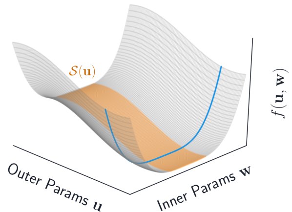
(a)

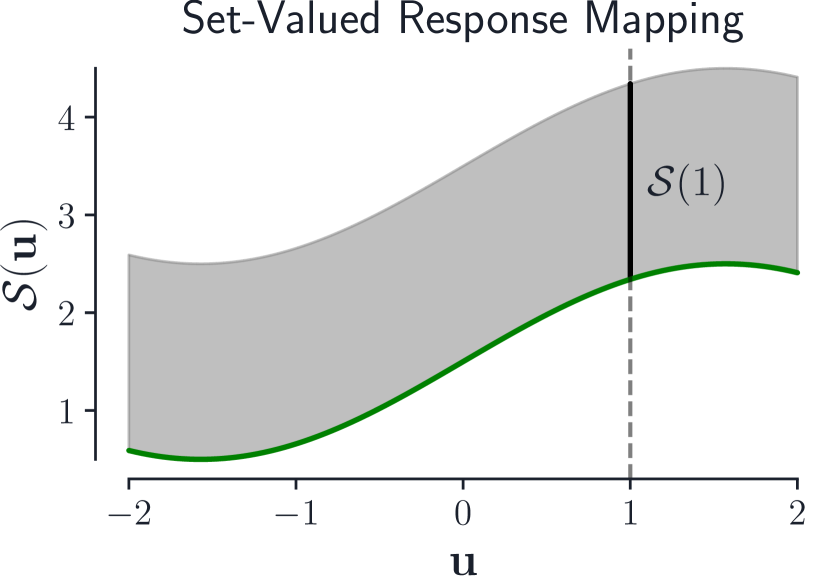
(b)

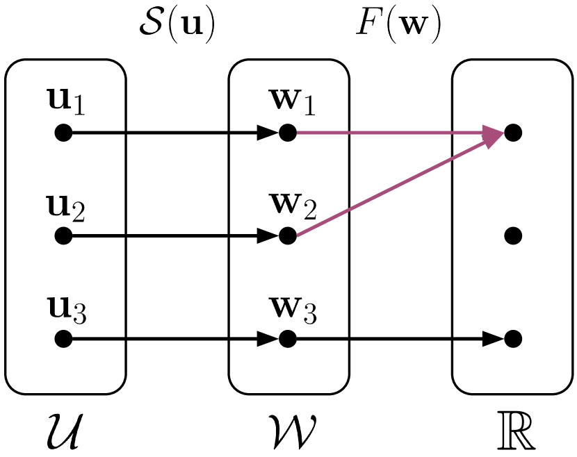
(c)

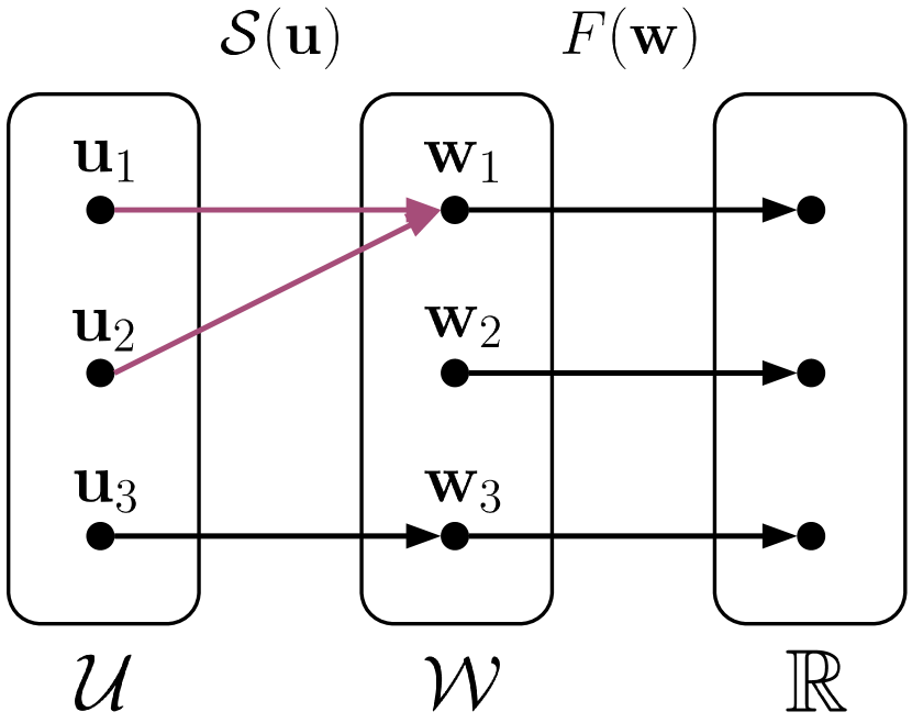
(d)

Figure 1: Underspecification in BLO. (a) Simplified visualization of inner underspecification, yielding a manifold of optimal solutions $\mathcal{S}(\mathbf{u})=\operatorname*{arg\,min}_{\mathbf{w}}f(\mathbf{u},\mathbf{w})$ for each $\mathbf{u}$ (a slice is highlighted in blue for a fixed $\mathbf{u}$). The orange region along the floor of the valley highlights the set-valued best-response mapping. (b) The set-valued best-response for $\mathbf{u},\mathbf{w}\in\mathbb{R}$, where the shaded gray region contains values of $\mathbf{w}$ that achieve equivalent performance on the inner objective. The green curve highlights the minimum-norm inner solutions for each $\mathbf{u}$. (c) Outer underspecification due to $F$ mapping a range of inner parameters to the same value; or (d) from $\mathcal{S}(\mathbf{u})$ associating a range of outer parameters with the same inner parameters.

Most algorithmic contributions to BLO make the simplifying assumption that the inner problem has a unique solution (e.g., $|\mathcal{S}(\mathbf{u})|=1,\forall\mathbf{u}\in\mathcal{U}$), and give approximation methods that provably get close to the solution (Shaban et al., 2019; Pedregosa, 2016; Yang et al., 2021; Hong et al., 2020; Grazzi et al., 2020a). In practice, however, these algorithms are often run in settings where either the inner or outer problem is underspecified; i.e., the set of optima forms a non-trivial manifold. Underspecification often occurs due to overparameterization, e.g., given a learning problem with more parameters than datapoints, there are typically infinitely many solutions that achieve the optimal objective value (Belkin, 2021). Analyses of the dynamics of overparameterized single-objective optimization have shown that the nature of the converged solution, such as its pattern of generalization, depends in subtle ways on the details of the optimization dynamics (Lee et al., 2019; Arora et al., 2019; Bartlett et al., 2020; Amari et al., 2020); this general phenomenon is known as implicit bias. We extend this investigation to the bilevel setting: What are the implicit biases of practical BLO algorithms? What types of solutions do they favor, and what are the implications for how the trained models behave?

Task	Inner ($\mathbf{w}$)	Outer ($\mathbf{u}$)	Inner Overparam	Outer Overparam
Dataset Distillation (Wang et al., 2018)	NN weights	Synthetic data	✓	✗
Data Augmentation (Hataya et al., 2020b)	NN weights	Augmentation params	✓	✗
GANs (Goodfellow et al., 2014)	Discriminator	Generator	✓	✓
Meta-Learning (Finn et al., 2017)	NN weights	NN weights	✓	✓
NAS (Liu et al., 2019)	NN weights	Architectures	✓	✓
Hyperopt (Maclaurin et al., 2015)	NN weights	Hyperparams	✓	✗
Example reweighting (Ren et al., 2018)	NN weights	Example weights	✓	✓

Table 1: Inner and outer overparameterization in common bilevel tasks. For each task, we reference whether the common use-case includes inner overparametrization and/or outer overparametrization (InnerU/OuterU).

We identify two sources of implicit bias in underspecified BLO: 1) bias resulting from the optimization algorithm, either cold-start or warm-start BLO (described below); and 2) bias resulting from the hypergradient approximation. Classic literature on bilevel optimization (Dempe, 2002) considers two ways to break ties between solutions in the set $\mathcal{S}(\mathbf{u})$: optimistic and pessimistic equilibria (discussed in Section 2). However, as we will show, neither describes the solutions obtained by the most common BLO algorithms. We focus on two algorithms that are relevant for practical machine learning, which we term cold-start and warm-start BLO. Cold-start BLO (Maclaurin et al., 2015; Metz et al., 2019; Micaelli & Storkey, 2020) defines the inner solution $\mathbf{w}^{\star}$ as the fixpoint of an update rule, which captures the notion of running an optimization algorithm to convergence. For each outer update, the inner parameters are re-initialized to $\mathbf{w}_{0}$ and the inner optimization is run from scratch. This is computationally expensive, as it requires full unrolls of the inner optimization for each outer step. Warm-start BLO is a more tractable and widely-used alternative (Luketina et al., 2016; MacKay et al., 2019; Lorraine et al., 2020; Tang et al., 2020) that alternates gradient descent steps on the inner and outer parameters: in each step of warm-start BLO, the inner parameters are optimized from their current values, rather than the initialization $\mathbf{w}_{0}$.

In Section 3, we characterize solution concepts that capture the behavior of the cold- and warm-start BLO algorithms and show that, for quadratic inner and outer objectives, cold-start BLO yields minimum-norm outer parameters. In Section 4, we show that warm-start BLO induces an implicit bias on the inner parameter iterates, regularizing the updates to maintain proximity to previous solutions. In addition to the BLO algorithm, another source of implicit bias is the hypergradient approximation. In Sections 3 and 4, we investigate the effect of using approximate implicit differentiation to compute the hypergradient $\frac{dF}{d\mathbf{u}}$, where different approximations can lead to vastly different outer solutions. In this paper, we consider both inner and outer underspecification.

Inner Underspecification.

Many bilevel tasks in machine learning train a neural network in the inner level, which typically yields an underspecified problem, as shown in Table 1. Figure 1(a,b) illustrates set-valued response mappings in underspecified BLO.

Outer Underspecification.

Outer underspecification can arise in two ways: either 1) the mapping $\mathcal{S}(\mathbf{u})$ is a function (e.g., not set-valued) and maps a range of outer parameters to the same inner parameter; or 2) the outer objective $F$ maps a range of inner parameters to the same objective value. These two pathways are illustrated in Figure 1(c,d).

Our code is available on Github, and we provide a Colab notebook here.

2 Background

In this section, we provide an overview of several key concepts that we build on in this paper. First, we review two methods for computing approximate hypergradients: differentiation through unrolling and implicit differentiation. Then, we discuss optimistic and pessimistic BLO, which are two existing solution concepts for problems with non-unique inner solutions, that differ in how they break ties among equally-valid inner parameters. Finally, we describe the task of dataset distillation, which we use for our empirical investigations in Section 4.

Hypergradient Approximation.

We assume that $F$ and $f$ are differentiable, and consider gradient-based BLO algorithms, which require the hypergradient $\frac{dF(\mathbf{u},\mathbf{w}_{\mathbf{u}}^{\star})}{d\mathbf{u}}=\frac{\partial F(\mathbf{u},\mathbf{w}_{\mathbf{u}}^{\star})}{\partial\mathbf{u}}+\left(\frac{d\mathbf{w}_{\mathbf{u}}^{\star}}{d\mathbf{u}}\right)^{\top}\frac{\partial F(\mathbf{u},\mathbf{w}_{\mathbf{u}}^{\star})}{\partial\mathbf{w}_{\mathbf{u}}^{\star}}$. The main challenge to computing the hypergradient lies in computing the response Jacobian $\frac{d\mathbf{w}_{\mathbf{u}}^{\star}}{d\mathbf{u}}$, which captures how the converged inner parameters depend on the outer parameters. Exactly computing this Jacobian is often intractable for large-scale problems. The two most common approaches to approximate it are: 1) iterative differentiation, which unrolls the inner optimization to reach an approximate best-response (BR) and backpropagates through the unrolled computation graph to compute the approximate BR Jacobian (Domke, 2012; Maclaurin et al., 2015; Shaban et al., 2019); and 2) implicit differentiation, which leverages the implicit function theorem (IFT) to compute the BR Jacobian, assuming that the inner parameters are at a stationary point of the inner objective (Larsen et al., 1996; Chen & Hagan, 1999; Bengio, 2000; Foo et al., 2008; Pedregosa, 2016; Lorraine et al., 2020; Hataya et al., 2020b; Raghu et al., 2020). The IFT states that, assuming uniqueness of the inner solution and under certain regularity conditions, we can compute the response Jacobian as $\frac{\partial\mathbf{w}^{\star}_{\mathbf{u}}}{\partial\mathbf{u}}=\left(\frac{\partial^{2}f}{\partial\mathbf{w}\partial\mathbf{w}^{\top}}\right)^{-1}\frac{\partial^{2}f}{\partial\mathbf{w}\partial\mathbf{u}}$. The term inside the inverse is the Hessian of the inner objective, which is typically intractable to store or invert directly (as neural nets can easily have millions of parameters). Thus, multiplication by the inverse Hessian is typically approximated using an iterative linear solver, such as truncated conjugate gradient (CG) (Pedregosa, 2016), GMRES (Blondel et al., 2021), or the Neumann series (Liao et al., 2018; Lorraine et al., 2020). The (un-truncated) Neumann series for an invertible Hessian $\frac{\partial^{2}f}{\partial\mathbf{w}\partial\mathbf{w}^{\top}}$ is defined as:

$$\left(\frac{\partial^{2}f}{\partial\mathbf{w}\partial\mathbf{w}^{\top}}\right)^{-1}=\alpha\sum_{j=0}^{\infty}\left(\mathbf{I}-\alpha\frac{\partial^{2}f}{\partial\mathbf{w}\partial\mathbf{w}^{\top}}\right)^{j}\,.$$ (2)

This series is known to converge when the largest eigenvalue of $\mathbf{I}-\alpha\frac{\partial^{2}f}{\partial\mathbf{w}\partial\mathbf{w}^{\top}}$ is $<$ 1. In practice, the Neumann series is typically truncated to the first $K$ terms.  Lorraine et al. (2020) showed that differentiating through $K$ steps of unrolling starting from optimal inner parameters $\mathbf{w}^{\star}$ is equivalent to approximating the inverse Hessian with the first $K$ terms in the Neumann series, a result we review in Appendix E. Approximate implicit differentiation can be implemented with efficient Hessian-vector products using modern autodiff libraries (Pearlmutter, 1994; Abadi et al., 2015; Paszke et al., 2017; Bradbury et al., 2018). However, when the inner problem is overparameterized, the Hessian $\frac{\partial^{2}f}{\partial\mathbf{w}\partial\mathbf{w}^{\top}}$ is singular. In Section 3, we discuss how the $K$-term truncated Neumann series approximates the inverse of the damped Hessian $(\mathbf{H}+\epsilon\mathbf{I})^{-1}$ (which is always non-singular), and we discuss the implications of this approximation.

Response Jacobians for Overparameterized Problems.

Let $\mathbf{H}=\frac{\partial^{2}f(\mathbf{u},\mathbf{w})}{\partial\mathbf{w}\partial\mathbf{w}^{\top}}$, $\mathbf{M}=\frac{\partial^{2}f(\mathbf{u},\mathbf{w})}{\partial\mathbf{u}\partial\mathbf{w}}$, and $\mathbf{J}=\frac{\partial\mathbf{w}_{\mathbf{u}}}{\partial\mathbf{u}}$. Then, for $\mathbf{w}_{\mathbf{u}}\in\operatorname*{arg\,min}_{\mathbf{w}}f(\mathbf{u},\mathbf{w})$, we have $\mathbf{H}\mathbf{J}=\mathbf{M}$. If $\mathbf{H}$ is invertible, then the unique response Jacobian is $\mathbf{J}=\mathbf{H}^{-1}\mathbf{M}$. However, when the inner problem is overparameterized, $\mathbf{H}$ is singular, and the Jacobian is not uniquely defined—it may be any matrix $\mathbf{J}$ satisfying $\mathbf{H}\mathbf{J}=\mathbf{M}$. If $\mathbf{J}$ is one such solution, then $\mathbf{J}+\mathbf{Z}$ is also a solution, where each column of $\mathbf{Z}$ is in the nullspace of $\mathbf{H}$. In this case, we define the canonical response Jacobian to be $\mathbf{J}=\mathbf{H}^{+}\mathbf{M}$, where $\mathbf{H}^{+}$ denotes the Moore-Penrose pseudoinverse of $\mathbf{H}$. This is the matrix with minimum Frobenius norm out of all solutions to the linear system (see Appendix B.1). We refer to the hypergradient computed using this canonical response Jacobian as the “exact” hypergradient.

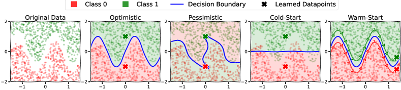
Figure 2: Dataset distillation sketch illustrating four solution concepts for BLO: optimistic, pessimistic, cold-start, and warm-start. We distill the dataset consisting of red and green points into two synthetic datapoints denoted by ✖ and ✖ (one per class). The learned datapoints ✖ and ✖ are the outer parameters, and the inner parameters correspond to a model (classifier) trained on these synthetic datapoints. We assume an overparameterized inner model, which can fit the synthetic datapoints with many different decision boundaries. All of the solutions here correctly classify the synthetic datapoints (and are thus valid solutions to the inner problem) but they differ in their behavior on the original dataset. Optimistic: finds the decision boundary that correctly classifies all the original datapoints; Pessimistic: finds the decision boundary that achieves the worst loss on the original datapoints—it correctly classifies the synthetic datapoints but incorrectly classifies the original datapoints (note the flipped red/green shading on either side of the decision boundary); Cold-start: finds the min-norm solution that correctly classifies the synthetic datapoints; Warm-start: yields a trajectory of synthetic datapoints over time, which can allow for a model trained on two learned datapoints to fit the original data.

Optimistic and Pessimistic BLO.

For scenarios where the inner problem has multiple solutions, i.e., $|\mathcal{S}(\mathbf{u})|>1$, two solution concepts have been widely studied in the classical BLO literature: the optimistic (Sinha et al., 2017; Dempe et al., 2007; Dempe, 2002; Harker & Pang, 1988; Lignola & Morgan, 1995; 2001; Outrata, 1993) and pessimistic (Sinha et al., 2017; Dempe, 2002; Dempe et al., 2014; Loridan & Morgan, 1996; Lucchetti et al., 1987; Wiesemann et al., 2013; Liu et al., 2018; 2020) solutions. In optimistic BLO, $\mathbf{w}$ is chosen such that it leads to the best outer objective value. In contrast, in pessimistic BLO, $\mathbf{w}$ is chosen such that it leads to the worst outer objective value. The corresponding equilibria are defined below, with the differences highlighted in purple and teal.

Dataset Distillation.

Given an original (typically large) dataset, the task of dataset distillation (Maclaurin et al., 2015; Wang et al., 2018; Lorraine et al., 2020) is to learn a smaller synthetic dataset such that a model trained on the synthetic data generalizes well to the original data. In this problem, the inner parameters are the weights of a model, and the outer parameters are the synthetic datapoints. The inner objective is the loss of the inner model trained on the synthetic datapoints, and the outer objective is the loss of the inner model on the original dataset:

We focus on dataset distillation throughout this paper because the degree of inner and outer overparameterization can be modified by varying the number of original versus synthetic datapoints. The solutions for this task are also easy to visualize and interpret.

Visualizing Solution Concepts.

Figure 2 illustrates four different solution concepts for a toy 2D problem: the optimistic and pessimistic solutions, as well as two new solution concepts—cold- and warm-start equilibria—that we discuss in Section 3. We consider dataset distillation for binary classification, with red and green datapoints representing the two classes, and a sinusoidal ground-truth decision boundary. We distill this dataset into two synthetic datapoints, represented by ✖ and ✖. In each subplot, the blue curve shows the decision boundary of the inner classifier, and the background colors show which class is predicted on each side of the decision boundary. See the caption of Figure 2 for a description of each solution concept on this task.

The optimistic solution can be tractable to compute (Mehra & Hamm, 2019; Ji & Liang, 2021), while the pessimistic solution is known to be less tractable (Sinha et al., 2017). From Figure 2, however, it is unclear whether either of these solution concepts is useful. For example, in hyperparameter optimization, the optimistic and pessimistic solutions correspond to choosing hyperparameters such that the inner training loop achieves minimum or maximum performance on the validation set, and it is unclear why this would be beneficial. Most widely-used BLO algorithms do not aim to find either of these solution concepts, which motivates our study of the behavior of the algorithms used in practice.

2.1 Algorithms

Here, we provide the algorithms for cold-start (Algorithm 1) and warm-start (Algorithm 2) bilevel optimization. Each algorithm can make use of different hypergradient approximations, including implicit differentiation with the truncated Neumann series (Algorithm 6), implicit differentiation with the damped Hessian inverse (Algorithm 5), and differentiation through unrolling (Algorithm 4).

Algorithm 1 Cold-Start BLO

1:Input: $\alpha$: inner LR, $\beta$: outer LR

2:           $T$: number of inner optimization steps

3:           $K$: number of Neumann series terms

4:while $||\hat{\nabla}_{\mathbf{u}}F(\mathbf{u},\mathbf{w})||^{2}>0$, iteration $t$ do

5:     $\hat{\nabla}_{\mathbf{u}}F\leftarrow\text{HypergradApprox}(\mathbf{u}_{t},{\color[rgb]{0,1,1}\mathbf{w}_{0}},T,K)$

6:     $\mathbf{u}_{t+1}\leftarrow\mathbf{u}_{t}-\beta\hat{\nabla}_{\mathbf{u}}F$

7:     

8:end while

9:return $(\mathbf{u}_{t},{\color[rgb]{0,1,1}\text{Optimize}(\mathbf{u}_{t},\mathbf{w}_{0},T)})$

Algorithm 2 Warm-start BLO

1:Input: $\alpha$: inner LR, $\beta$: outer LR

2:           $T$: number of inner optimization steps

3:           $K$: number of Neumann series terms

4:while $||\hat{\nabla}_{\mathbf{u}}F(\mathbf{u},\mathbf{w})||^{2}>0$, iteration $t$ do

5:     $\hat{\nabla}_{\mathbf{u}}F\leftarrow\text{HypergradApprox}(\mathbf{u}_{t},{\color[rgb]{1,.5,0}\mathbf{w}_{t}},T,K)$

6:     $\mathbf{u}_{t+1}\leftarrow\mathbf{u}_{t}-\beta\hat{\nabla}_{\mathbf{u}}F$

7:     $\mathbf{w}_{t+1}\leftarrow\text{Optimize}(\mathbf{u}_{t+1},\mathbf{w}_{t},T)$

8:end while

9:return $(\mathbf{u}_{t},{\color[rgb]{1,.5,0}\mathbf{w}_{t}})$

Figure 3: Algorithms for cold-start and warm-start bilevel optimization. We highlight the key differences in cyan for cold-start and orange for warm-start. HypergradApprox is a placeholder for one of three different algorithms: 1) NeumannHypergrad (Algorithm 6), which computes the hypergradient using the IFT with the Neumann series approximation of the inverse Hessian; 2) DampedHypergrad (Algorithm 5), which similarly uses the IFT with the damped Hessian inverse $(\mathbf{H}+\epsilon\mathbf{I})^{-1}$; or 3) IterDiffHypergrad (Algorithm 4), which computes the hypergradient by differentiating through unrolled inner optimization.

Algorithm 3 $\textnormal{Optimize}(\mathbf{u},\mathbf{w},T)$

1:Input: $\gamma$: learning rate

2:           $T$: unroll steps

3:           $\mathbf{w}$: initialization

4:for $t=1,\dots,T$ do

5:     $\mathbf{w}\leftarrow\mathbf{w}-\gamma\nabla_{\mathbf{w}}f(\mathbf{u},\mathbf{w})$

6:end for

7:return $\mathbf{w}$

Algorithm 4 IterDiffHypergrad

1:Input: $\alpha$: inner LR

2:           $\beta$: outer LR

3:           $T$: inner steps

4:$\hat{\mathbf{w}}_{T}^{*}\leftarrow\text{Optimize}(\mathbf{u}_{t},\mathbf{w}_{t},T)$

5:$\hat{F}\leftarrow F(\mathbf{u},\hat{\mathbf{w}}^{*}_{T})$

6:Compute $\nabla_{\mathbf{u}}\hat{F}$ using auto-diff.

Figure 4: Helper functions to compute the implicit hypergradient using the Neumann series to approximate the inverse inner loss Hessian.

Algorithm 5 DampedHypergrad

1:Input: $\alpha$: inner LR

2:           $\beta$: outer LR

3:           $T$: inner steps

4:            $\epsilon$: damping coeff.

5:$\hat{\mathbf{w}}_{T}^{*}\leftarrow\text{Optimize}(\mathbf{u}_{t},\mathbf{w}_{t},T)$

6:$\mathbf{A}\leftarrow\left(\frac{\partial^{2}f(\mathbf{u}_{t},\hat{\mathbf{w}}_{T}^{*})}{\partial\mathbf{w}\partial\mathbf{w}^{\top}}+\epsilon\mathbf{I}\right)^{-1}$

7:$\mathbf{M}\leftarrow\frac{\partial^{2}f(\mathbf{u}_{t},\hat{\mathbf{w}}_{T}^{*})}{\partial\mathbf{u}\partial\mathbf{w}}$

8:$\frac{d\hat{\mathbf{w}}_{T}^{*}}{d\mathbf{u}}\leftarrow\mathbf{A}\mathbf{M}$

9:$\hat{\nabla}_{\mathbf{u}}F\leftarrow\frac{\partial F}{\partial\mathbf{u}}+\left(\frac{d\hat{\mathbf{w}}_{T}^{*}}{d\mathbf{u}}\right)^{\top}\frac{\partial F(\mathbf{u},\hat{\mathbf{w}}_{T}^{*})}{\partial\hat{\mathbf{w}}_{T}^{*}}$

10:return $\hat{\nabla}_{\mathbf{u}}F$

Algorithm 6 NeumannHypergrad

1:Input: $\alpha$: inner LR

2:           $\beta$: outer LR

3:           $T$: inner steps

4:           $K$: Neumann terms

5:$\hat{\mathbf{w}}_{T}^{*}\leftarrow\text{Optimize}(\mathbf{u}_{t},\mathbf{w}_{t},T)$

6:$\frac{d\hat{\mathbf{w}}_{T}^{*}}{d\mathbf{u}}\leftarrow\alpha\sum_{j=0}^{K}\left(\mathbf{I}-\alpha\frac{\partial^{2}f(\mathbf{u},\mathbf{w})}{\partial\mathbf{w}\partial\mathbf{w}^{\top}}\right)^{j}$

7:$\hat{\nabla}_{\mathbf{u}}F\leftarrow\frac{\partial F}{\partial\mathbf{u}}+\left(\frac{d\hat{\mathbf{w}}_{T}^{*}}{d\mathbf{u}}\right)^{\top}\frac{\partial F(\mathbf{u},\hat{\mathbf{w}}_{T}^{*})}{\partial\hat{\mathbf{w}}_{T}^{*}}$

8:return $\hat{\nabla}_{\mathbf{u}}F$

Figure 5: DampedHypergrad uses the IFT with the damped Hessian inverse $(\mathbf{H}+\epsilon\mathbf{I})^{-1}$ and IterDiffHypergrad unrolls the inner optimization and backpropagates through the unroll.

3 Equilibrium Concepts

We aim to understand the behavior of two popular BLO algorithms: cold-start (Algorithm 1) and warm-start (Algorithm 2). A summary of the updates for each algorithm is shown in Table 2. In this section, we first define equilibrium notions that capture the solutions found by warm-start and cold-start BLO. We then discuss properties of these equilibria, in particular focusing on the norms of the resulting inner and outer parameters. Finally, we analyze the implicit bias induced by approximating the hypergradient with the truncated Neumann series.

3.1 Cold-Start Equilibrium

Here, we introduce a solution concept that captures the behavior of cold-start BLO. We consider an iterative optimization algorithm used to compute an approximate solution to the inner objective. We denote a step of inner optimization by $\mathbf{w}_{t+1}=\Xi(\mathbf{u},\mathbf{w}_{t})$; for gradient descent, we have $\Xi(\mathbf{u},\mathbf{w}_{t})=\mathbf{w}_{t}-\alpha\nabla_{\mathbf{w}}f(\mathbf{u},\mathbf{w}_{t})$. We denote $K$ steps of inner optimization from $\mathbf{w}_{0}$ by $\Xi^{(K)}(\mathbf{u},\mathbf{w}_{0})$. Under certain assumptions (e.g., that $f$ has a unique finite root and that the step size $\alpha$ for the update is chosen appropriately), repeated application of $\Xi$ will converge to a fixpoint. We denote the fixpoint for an initialization $\mathbf{w}_{0}$ by $\Xi^{(\infty)}(\mathbf{u},\mathbf{w}_{0})$.

In some cases, we can compute the fixpoint of the inner optimization analytically. In particular, when $f$ is quadratic, the analytic solution minimizes the displacement from $\mathbf{w}_{0}$: $\Xi^{(\infty)}(\mathbf{u},\mathbf{w}_{0})=\operatorname*{arg\,min}_{\mathbf{w}\in\mathcal{S}(\mathbf{u})}\|\mathbf{w}-\mathbf{w}_{0}\|_{2}^{2}$.

3.2 Warm-Start Equilibrium

Next, we introduce a solution concept intended to capture the behavior of warm-start BLO. Warm-starting refers to initializing the inner optimization from the inner parameters obtained in the previous hypergradient computation. One can consider two variants of warm-starting: (1) using full inner optimization, that is, running the inner optimization to convergence starting from $\mathbf{w}_{t}$ to obtain the next iterate $\mathbf{w}_{t+1}$; or (2) partial inner optimization, where we approximate the solution to the inner problem via a few gradient steps.

Method	Inner Update
Full Cold-Start	$\mathbf{w}^{\star}_{k+1}=\Xi^{(\infty)}(\mathbf{u}_{k+1},\mathbf{w}_{0})$
Full Warm-Start	$\mathbf{w}^{\star}_{k+1}=\Xi^{(\infty)}(\mathbf{u}_{k+1},\mathbf{w}_{k}^{\star})$
Partial Warm-Start	$\mathbf{w}^{\star}_{k+1}=\Xi^{(T)}(\mathbf{u}_{k+1},\mathbf{w}_{k}^{\star})$

Table 2: Inner parameter updates for cold-start, full warm-start, and partial warm-start BLO.

Full warm-start can be expressed as computing $\mathbf{w}_{k+1}^{\star}=\Xi^{(\infty)}(\mathbf{u},\mathbf{w}_{k}^{\star})$ in each iteration, starting from the previous inner solution $\mathbf{w}_{k}^{\star}$ rather than $\mathbf{w}_{0}$. Similarly, partial warm-start can be expressed as $\mathbf{w}_{k+1}^{\star}=\Xi^{(T)}(\mathbf{u},\mathbf{w}_{k}^{\star})$, where $T$ is often small (e.g., $T<10$).

3.3 Solution Properties

In this section, we examine properties of cold-start and warm-start equilibria—we analyze the norms of the inner and outer parameters given by different methods. First, we show that, when $F$ and $f$ are quadratic, cold-start equilibria yield minimum-norm outer parameters. Then, we analyze the implicit bias induced by the hypergradient approximation, in particular by using the truncated Neumann series to estimate the inverse Hessian for implicit differentiation. To make the analysis tractable, we make the following assumption:

We assume that the inner objective is a convex (but not strongly-convex) quadratic, which may have many global minima, providing a tractable setting to analyze implicit bias. This allows us to model an overparameterized linear regression problem with data matrix $\boldsymbol{\Phi}\in\mathbb{R}^{n\times p}$, which corresponds to a quadratic with curvature $\boldsymbol{\Phi}^{\top}\boldsymbol{\Phi}$. When the number of parameters is greater than the number of training examples ($p>n$), $\boldsymbol{\Phi}^{\top}\boldsymbol{\Phi}$ is PSD. In this case, $f$ has a manifold of valid solutions (Wu & Xu, 2020).

Implicit Bias of Cold-Start for Inner Solutions.

Because cold-start BLO optimizes the inner parameters from initialization to convergence for each outer iteration, the inner solution inherits properties from the single-level optimization literature. For example, in linear regression trained with gradient descent, the inner solution will minimize displacement from the initialization $\left|\left|\mathbf{w}-\mathbf{w}_{0}\right|\right|_{2}^{2}$. Recent work aims to generalize such statements to other model classes and optimization algorithms—e.g., obtaining min-norm solutions with algorithm-specific norms (Gunasekar et al., 2018). Generalizing the results for various types of neural nets is an active research area (Vardi & Shamir, 2021).

Implicit Bias of Cold-Start for Outer Solutions.

In the following theorem, we show that cold-start BLO from outer initialization $\mathbf{u}_{0}$, converges to the outer solution $\mathbf{u}^{\star}$ that minimizes displacement from $\mathbf{u}_{0}$.

Next, we observe that the full warm-start and cold-start algorithms are equivalent for strongly-convex inner problems.

We relate partial and full warm-start equilibria as follows:

3.3.1 Implicit Bias from Hypergradient Approximation

Neumann Series.

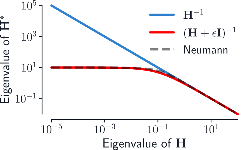
Figure 6: Eigenvalues of various matrix functions of $\mathbf{H}$ (denoted $\mathbf{H}^{\star}$ in the diagram): $\mathbf{H}^{-1}$, $(\mathbf{H}+\epsilon\mathbf{I})^{-1}$, and the Neumann series approximation $\alpha\sum_{j=0}^{K}(\mathbf{I}-\alpha\mathbf{H})^{j}$. Here, $\epsilon=\frac{1}{\alpha K}$.

Next, we investigate the impact of the hypergradient approximation on the converged outer solution. In practice, one often uses the truncated Neumann series to estimate the inverse Hessian when computing the implicit hypergradient. Note that:

where $\epsilon=\frac{1}{\alpha K}$. This is known from the spectral regularization literature (Gerfo et al., 2008; Rosasco, 2009). We show in Appendix D that the damped Hessian inverse $(\mathbf{H}+\epsilon\mathbf{I})^{-1}$ corresponds to the hypergradient of a proximally-regularized inner objective: $\hat{f}(\mathbf{u},\mathbf{w})=f(\mathbf{u},\mathbf{w})+\frac{\epsilon}{2}\|\mathbf{w}-\mathbf{w}^{\prime}\|_{2}^{2}$, where $\mathbf{w}^{\prime}\in\operatorname*{arg\,min}_{\mathbf{w}}f(\mathbf{u},\mathbf{w})$. The damping prevents the inner optimization from moving far in low-curvature directions. Consider the spectral decomposition of the real symmetric matrix $\mathbf{H}=\mathbf{U}\mathbf{D}\mathbf{U}^{\top}$, where $\mathbf{D}$ is a diagonal matrix containing the eigenvalues of $\mathbf{H}$, and $\mathbf{U}$ is an orthogonal matrix. Then, $(\mathbf{H}+\epsilon\mathbf{I})^{-1}=(\mathbf{U}\mathbf{D}\mathbf{U}^{\top}+\epsilon\mathbf{I})^{-1}=(\mathbf{U}(\mathbf{D}+\epsilon\mathbf{I})\mathbf{U}^{\top})^{-1}=\mathbf{U}^{\top}(\mathbf{D}+\epsilon\mathbf{I})^{-1}\mathbf{U}$. If $\lambda$ is an eigenvalue of $\mathbf{H}$, then the corresponding eigenvalue of $\mathbf{H}^{-1}$ is $\frac{1}{\lambda}$. In contrast, the corresponding eigenvalue of $(\mathbf{H}+\epsilon\mathbf{I})^{-1}$ is $\frac{1}{\lambda+\epsilon}$. When $\epsilon\ll\lambda$, $\frac{1}{\lambda+\epsilon}\approx\frac{1}{\lambda}$; when $\lambda\ll\epsilon$, $\frac{1}{\lambda+\epsilon}\approx\frac{1}{\epsilon}$. Thus, the influence of small eigenvalues (associated with low-curvature directions) is diminished, and the truncated Neumann series primarily takes into account high-curvature directions. Figure 6 illustrates the relationship between the eigenvalues of $\mathbf{H}^{-1}$, $(\mathbf{H}+\epsilon\mathbf{I})^{-1}$, and $\alpha\sum_{j=0}^{K}(\mathbf{I}-\alpha\mathbf{H})^{j}$.

Unrolling.

The implicit bias induced by approximating the hypergradient via $K$-step unrolled differentiation is qualitatively similar to the bias induced by the truncated Neumann series. For quadratic inner objectives $f$, the truncated Neumann series coincides with the result of differentiating through $K$ steps of unrolled gradient descent, because the Hessian of a quadratic is constant over the inner optimization trajectory (Lorraine et al., 2020). Note that gradient descent on a quadratic converges (for step-size $\alpha\leq 1/\|\mathbf{H}\|_{2}$) more rapidly in high-curvature directions than in low-curvature directions. Thus, the approximate best response obtained by truncated unrolling only takes into account high-curvature directions of the inner objective, and is less sensitive to low-curvature directions. In turn, the response Jacobian will only capture how the inner parameters depend on the outer parameters in these high-curvature directions. Note that for general objectives $f$ (e.g., when training neural networks), differentiating through unrolling only coincides with the Neumann series when the inner parameters are at a stationary point of $f$.

4 Empirical Overparameterization Results

Many large-scale empirical studies—in particular in the areas of hyperparameter optimization and data augmentation—use warm-start bilevel optimization (Hataya et al., 2020b; Ho et al., 2019; Mounsaveng et al., 2021; Peng et al., 2018; Tang et al., 2020). In this section, we introduce simple tasks based on dataset distillation, designed to provide insights into the phenomena at play. First, we show that when the inner problem is overparameterized, the inner parameters $\mathbf{w}$ can retain information associated with different settings of the outer parameters over the course of joint optimization. Then, we show that when the outer problem is overparameterized, the choice of hypergradient approximation can affect which outer solution is found. Experimental details and extended results are provided in Appendix F.

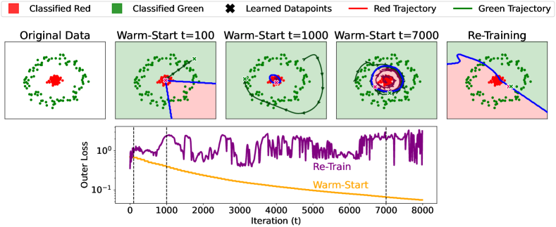
Figure 7: Dataset distillation for binary classification, with two learned datapoints (outer parameters) adapted jointly with the model weights (inner parameters). Top left: The original data distribution we wish to distill; Top middle three plots: Visualizations of snapshots during training with warm-start BLO, at iterations $t\in\{100,1000,7000\}$ (indicated by the dashed vertical lines in the bottom plot). In each middle figure, we plot the new portion of the synthetic datapoint trajectory since the previous snapshot, shown by a curve with arrows; Top right: Decision boundary when re-training to convergence on the final values of the two distilled datapoints yields a poor solution for the original data. Bottom: We show the outer loss over the course of a single run of warm-start BLO corresponding to the middle three plots in the top row. We also demonstrate that none of the intermediate synthetic datapoint pairs along the trajectory is sufficient to fit the original data well, by re-training on each intermediate point (shown by the purple curve).

4.1 Inner Overparameterization: Dataset Distillation

In dataset distillation, the original dataset is only accessed in the outer objective; thus, one might expect that the lower-dimensional distilled dataset would act as an information bottleneck between the objectives. Because the outer objective is only used directly to update the outer variables, it would seem intuitive that all of the information about the outer objective is compressed into the outer variables. While this is correct for the cold-start equilibrium, we show that it does not hold for the warm-start equilibrium: a surprisingly large amount of information can leak from the original dataset to the inner variables (e.g., network weights).

Consider a 2D binary classification task where the classes form concentric rings (Figure 7). We aim to learn two distilled datapoints (one per class) to model the circular decision boundary. One may a priori expect that this would not be possible when training an MLP on only the two distilled points; indeed, we observe poor decision boundaries for the original dataset when training a model to convergence on the synthetic datapoints (Figure 7, Top Right). However, when performing warm-start alternating updates on the MLP parameters and the learned datapoints, the datapoints follow a nontrivial trajectory, tracing out the decision boundary between classes over time (Figure 7, middle three plots). The model trained jointly with the two learned datapoints fits to the full trajectory of those datapoints. Thus, warm-started BLO yields a model that achieves nearly the same outer loss as one trained directly on the original data, despite only training on a single datapoint per class. See the caption of Figure 7 for details on interpreting this result. We provide additional results in Appendix F.1, where we consider the three-class variant of this problem: we show that similar results hold when learning three distilled datapoints (one per class), and even when learning just two distilled datapoints along with their soft labels—in which case one datapoint switches its label over the course of training.

Warm-Start Memory.

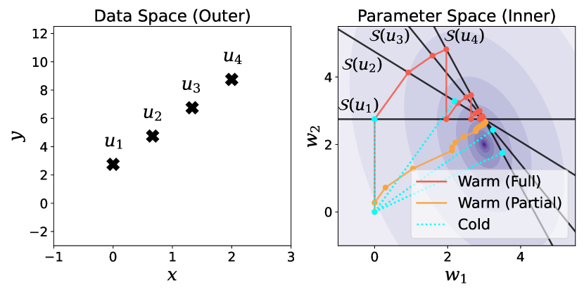
Figure 8: Sketch illustrating projection onto a fixed sequence of solution sets $\{\mathcal{S}(\mathbf{u}_{i})\}_{i=1}^{4}$, from different initializations. Warm-start with full inner optimization projects from one solution set to the next; warm-start with partial inner optimization takes a step in the direction towards each solution set; and cold-start re-projects from the origin.

Here we provide intuition for the warm-start behavior observed in Figure 7. In particular, we discuss how warm-start BLO can induce a memory effect. Figure 8 sketches warm- and cold-start algorithms on a toy example where we can visualize the steps of each algorithm in the inner parameter space. The solution sets for four fixed values of a single synthetic datapoint are shown by the solid black lines in Figure 8, and outer loss contours are shown in the background. The inner parameters are initialized at the origin. Due to the implicit bias of the inner optimization problem, in each iteration of cold-start BLO, the initial inner parameters $\mathbf{w}_{0}=\boldsymbol{0}$ are projected onto the solution set corresponding to the current outer parameter: $\mathbf{w}_{k+1}^{\star}=\Pi(\boldsymbol{0},\mathcal{S}(\mathbf{u}_{k}))$, where $\Pi(\cdot,\mathcal{C})$ denotes projection onto the (convex) set $\mathcal{C}$. In contrast, full warm-start projects the previous inner parameters onto the current solution set: $\mathbf{w}_{k+1}^{\star}=\Pi(\mathbf{w}_{k}^{\star},\mathcal{S}(\mathbf{u}_{k}))$. If one cycles through the solution sets repeatedly, then full warm-start BLO is equivalent to the Kaczmarz algorithm (Karczmarz, 1937), a classic alternating projection algorithm for finding a point in the intersection of the constraint sets (see Appendix B.2 for details). In this case, the inner parameters will converge to the intersection of the solution sets $\{\mathcal{S}(\mathbf{u}_{i})\}_{i=1}^{4}$, in effect yielding inner parameters that perform well for several outer parameters simultaneously. In the case of dataset distillation, this corresponds to model weights which fit all of the distilled datapoints over the outer optimization trajectory.

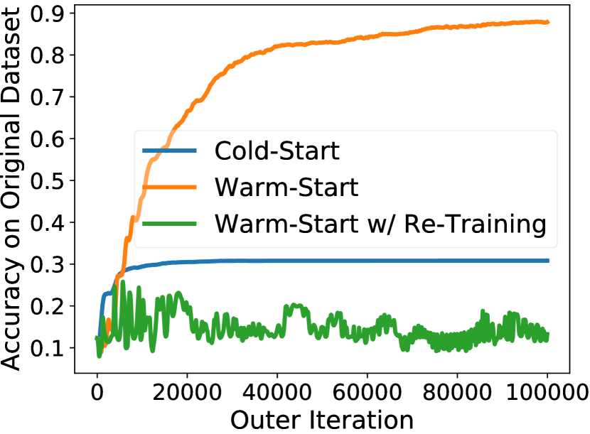
(a) Accuracies

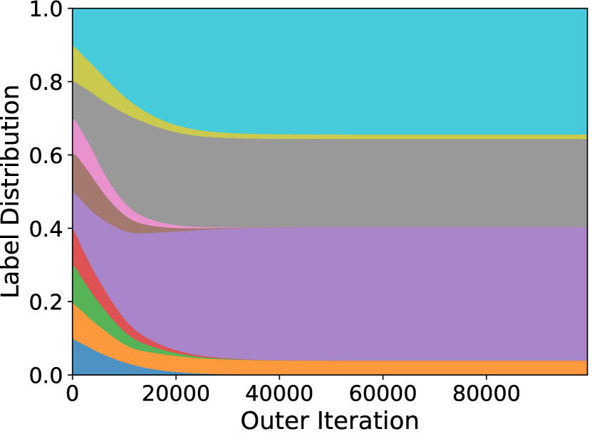
(b) Cold-start soft labels

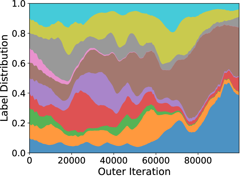
(c) Warm-start soft labels

Figure 9: MNIST dataset distillation using a linear classifier. Here, we learn a single synthetic datapoint (a $28\times 28$ image canvas) and corresponding soft label (a 10-dimensional vector representing class logits).

Warm-Start vs Cold-Start in High-Dimensions.

To illustrate warm-start phenomena in high-dimensional problems, we ran dataset distillation on MNIST using a linear classifier. The original dataset to be distilled consists of 10000 examples from the MNIST training set. The BLO methods are tasked with learning a single $28\times 28$ image canvas and a 10-dimensional vector of soft labels—e.g., the outer parameters are $28^{2}+10=794$ dimensional. Figure 9(a) shows the accuracy of the model on the original dataset, when optimizing a single synthetic datapoint and its soft label with warm-start, cold-start, and warm-start + re-training (which trains a model from scratch on the warm-start synthetic datapoint at the current outer iteration). We visualize the soft label evolution in Figures 9(b) and 9(c), showing classes 0-9 as colored regions. While the cold-start soft label quickly converges to a mixture of three classes, warm-start continues to adapt the soft label over the course of joint optimization, effectively training the inner model on all 10 classes (e.g., by placing more weight on different classes at different timesteps along the training trajectory). We obtained similar results on MNIST, FashionMNIST, and CIFAR-10, with 1 or 10 synthetic datapoints (see Table 3). In addition to dataset distillation, we observe similar phenomena in hyperparameter optimization. We trained a linear data augmentation (DA) network that transforms inputs before feeding them into a classifier; here, the DA net parameters are hyperparameters $\mathbf{u}$, tuned on the validation set. We used subsampled training sets consisting of 50 datapoints—so that data augmentation is beneficial—and evaluated performance on the full validation set. Table 3 compares warm- and cold-start BLO on this task. Note that in order to compare with cold-start solutions (which need $10^{3}$–$10^{4}$ inner optimization steps), we require tractable inner problems like linear models or MLPs.

	Dataset Distillation			Data Augmentation Net
Method	MNIST	Fashion	CIFAR-10	MNIST	Fashion	CIFAR-10
Cold-Start	30.7 / 89.1	33.2 / 83.0	17.6 / 46.9	84.86	84.04	45.38
Warm-Start	90.8 / 97.5	88.2 / 94.2	50.3 / 59.8	92.81	89.51	59.30
Warm-Start + Retraining	12.9 / 17.1	7.0 / 12.6	10.2 / 8.9	9.15	25.32	11.12

Table 3: Columns 1-3: Accuracy on original data with 1/10 synthetic samples. Columns 4-6: Learning a linear data augmentation network.

Warm-Start Takeaways.

Warm-start BLO yields outer parameters that fail to generalize under re-initialization of the inner problem. In both toy and high-dimensional problems, re-training with the final outer parameters (e.g., discarding the outer optimization trajectory) yields a model that performs poorly on the outer objective. In addition, warm-start BLO leaks information about the outer objective to the inner parameters, which can lead to overestimation of performance. For example, when adapting a small number of hyperparameters online, warm-start BLO may overfit the validation set, yielding a model that fails to generalize to the test set.

4.2 Outer Overparameterization: Anti-Distillation

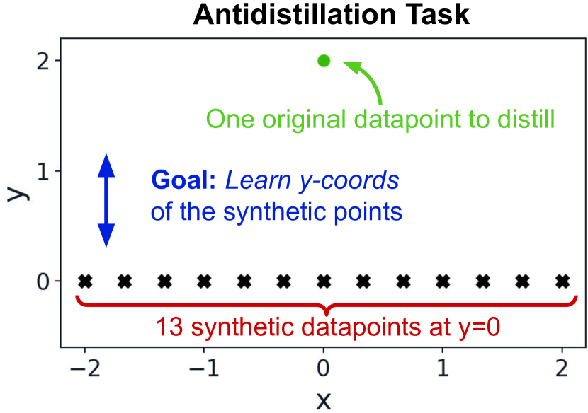
Figure 10: Antidistillation regression task setup.

In the previous section, we investigated implicit bias resulting from the choice of cold- vs warm-start BLO algorithms. Next, we focus on cold-start BLO, and show that when the outer problem is overparameterized, different hypergradient approximations can lead to vastly different outer solutions. In particular, we construct a simple problem that illustrates the impact of using the truncated Neumann series or damping to approximate the inverse Hessian when computing the hypergradient. We propose a task related to dataset distillation, but where we have more learned datapoints than original dataset examples, which we term anti-distillation (see Figure 10 for an illustration of the problem setup). Here, there are many valid ways to set the learned datapoints such that a model trained on those points achieves good performance on the original data: any solution that places one learned datapoint on top of the original point perfectly fits the outer objective.

Anti-Distillation.

Consider a regression task with inner objective $f(\mathbf{u},\mathbf{w})=\frac{1}{2}\|\mathbf{\Phi}\mathbf{w}-\mathbf{u}\|_{2}^{2}$, where the outer parameters $\mathbf{u}$ represent only the targets, not the inputs. The outer objective computes the loss on a fixed set of original datapoints $\{(x^{(o)}_{i},y^{(o)}_{i})\}_{i=1}^{P}$: $F(\mathbf{u},\mathbf{w})=\frac{1}{2}\|\mathbf{\Phi}^{(o)}\mathbf{w}-\mathbf{y}\|_{2}^{2}$. Here, $f$ and $F$ are quadratics that satisfy Assumption 3.1. The distillation task is to learn the $y$-coordinates of $N$ synthetic datapoints $\{(x_{i},y_{i})\}_{i=1}^{N}$ with fixed $x$-coordinates. The design matrix $\mathbf{\Phi}$ is $N\times D$, where each row is a $D$-dimensional feature vector given by the following Fourier basis mapping:

$$\boldsymbol{\phi}(x)=\begin{bmatrix}1&\smash{\underbrace{\begin{matrix}2^{L-1}\cos(x)&2^{L-2}\cos(2x)&\cdots&\cos(Lx)\end{matrix}}_{L\cos\text{terms}}}&\smash{\underbrace{\begin{matrix}2^{L-1}\sin(x)&2^{L-2}\sin(2x)&\cdots&\sin(Lx)\end{matrix}}_{L\sin\text{terms}}}\end{bmatrix}$$

We designed $\boldsymbol{\phi}(x)$ such that low-frequency terms have larger amplitudes than high-frequency terms, yielding an inductive bias for smoothness: it is easier (e.g., requires a smaller adjustment to the weights $\mathbf{w}$) to fit a given curve using the low-frequency terms than using the high-frequency terms. Thus, the minimum-norm solution found by gradient descent will explain as much as possible using low frequency terms. Note that neural networks have also been observed to have a bias towards low-frequency information (Basri et al., 2020; Rahaman et al., 2019; Tancik et al., 2020).

Hypergradient Approximations.

We consider the cold-start solution for the inner problem from initialization $\mathbf{w}_{0}=\boldsymbol{0}$, which can be computed analytically as $\mathbf{w}^{\star}=\mathbf{\Phi}^{+}\mathbf{u}$. At this inner solution, we compare three different methods to compute the hypergradient $\nabla_{\mathbf{u}}F(\mathbf{u},\mathbf{w})$, which differ in how they estimate the response Jacobian $\frac{\partial\mathbf{w}}{\partial\mathbf{u}}$: 1) differentiation through the closed-form, min-norm solution yields $\frac{\partial(\mathbf{\Phi}^{+}\mathbf{u})}{\partial\mathbf{u}}=\mathbf{\Phi}^{+}$; 2) implicit differentiation using the truncated, $K$-term Neumann series yields $\alpha\left(\sum_{j=0}^{K}(\mathbf{I}-\alpha\mathbf{H})^{j}\right)\mathbf{M}$; and 3) implicit differentiation using the damped Hessian inverse yields $(\mathbf{H}+\epsilon\mathbf{I})^{-1}\mathbf{M}$.

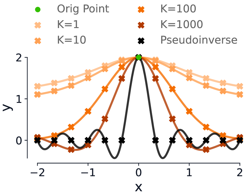
(a) Neumann/unrolling

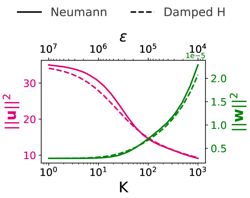
(b) Parameter norms

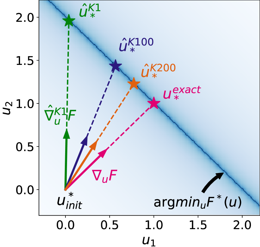
(c) Approx. hypergrads

Figure 11: Antidistillation task for linear regression with an overparameterized outer objective. We learn the $y$-component of 13 synthetic datapoints such that a regressor trained on those points will fit a single original dataset point, shown by the green dot at $(0,2)$. Fig. (a) shows the learned datapoints (outer parameters) obtained via different truncated Neumann approximations to the hypergradient. Fig. (b) shows the norms of the outer parameters $\|\mathbf{u}\|^{2}$ as a function of $K$ (for Neumann/unrolling) or $\epsilon$ (for the damped Hessian inverse). We observe that better hypergradient approximations (e.g., larger $K$ or smaller $\epsilon$) lead to smaller norm outer parameters, because they account for both high- and low-curvature directions of the inner objective. Fig. (c) visualizes outer optimization trajectories in the outer parameter space, to provide intuition for the behavior in (a) and (b). We consider antidistillation with 1 original datapoint and 2 learned datapoints. We show the true hypergradient $\nabla_{\mathbf{u}}F$, approximations using truncated Neumann series $\hat{\nabla}_{\mathbf{u}}F$, and the converged outer parameters for each setting, e.g., $\hat{\mathbf{u}}^{K1}_{\star}$.

Results.

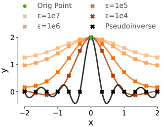
Figure 14: Antidistillation task for linear regression with an overparameterized outer objective. This plot uses the same setup as Figure 11, but shows learned datapoints obtained using the damped Hessian inverse $(\mathbf{H}+\epsilon\mathbf{I})^{-1}$ to compute the approximate hypergradient, for various damping factors $\epsilon$.

When we estimate the response Jacobian with a small number of steps of unrolling, the inner optimizer will do its best to fit the data using the low-frequency basis terms, which correspond to high-curvature directions of the inner loss. In Figure 11(a), we show the solutions obtained for different truncations of the Neumann series; also note that, because this problem is quadratic, the $K$-step unrolled hypergradient coincides with the $K$-step Neumann series hypergradient. To demonstrate the relationship $\alpha\sum_{j=0}^{K}(\mathbf{I}-\alpha\mathbf{H})^{j}\approx(\mathbf{H}+\frac{1}{\alpha K}\mathbf{I})^{-1}$ empirically, we also show the distilled datasets obtained with the damped inverse Hessian hypergradient approximation, for various damping factors $\epsilon\in\{\text{1e4, 1e5, 1e6, 1e7}\}$ (where $\epsilon=\frac{1}{\alpha K}$), in Appendix F.2 Figure 14, where we observe similar behavior to the Neumann series. In Figure 11(b) we plot the norms of the converged inner and outer parameters for a range of Neumann truncation lengths $K$ and damping factors $\epsilon$. We see that although they are not equivalent, the Neumann and damped Hessian approximate hypergradients behave similarly. In Appendix F, Figure 18, we show similar behavior when using an MLP rather than a linear model. Also note that this effect occurs in general for quadratic problems that are outer-overparameterized; it does not depend on inner overparameterization (see Appendix F.2).

Figure 11(c) visualizes optimization trajectories in the outer parameter space to provide additional intuition for the behavior of the outer parameter norms in Figure 11(b). We consider antidistillation with 1 original and 2 learned datapoints. We use $\hat{\nabla}_{\mathbf{u}}^{K}F(\mathbf{u},\mathbf{w})$ to denote the approximate hypergradient obtained via implicit differentiation with the $K$-term truncated Neumann series. We show the true hypergradient $\nabla_{\mathbf{u}}F$ (which we define in terms of the pseudoinverse), approximations using truncated Neumann series $\hat{\nabla}_{\mathbf{u}}F$, and the converged outer parameters for each setting, e.g., $\hat{\mathbf{u}}^{K1}_{\star}$. We observe that: 1) when the outer problem is overparameterized, approximate hypergradients converge to valid solutions in $\operatorname*{arg\,min}_{\mathbf{u}}F^{\star}(\mathbf{u})$; and 2) the exact hypergradient converges to the min-norm outer solution.

5 Related Work

Overparameterization.

Overparameterization has long been studied in single-level optimization, generating key insights such as neural network behavior in the infinite-width limit (Jacot et al., 2018; Sohl-Dickstein et al., 2020; Lee et al., 2019), double descent phenomena (Nakkiran et al., 2020; Belkin et al., 2019), the ability to fit random labels (Zhang et al., 2016), and the inductive biases of optimizers. However, prior work has not investigated implicit bias in bilevel optimization. While we focus quadratic problems, note that in single-level optimization, analyses based on the Neural Tangent Kernel (NTK) (Sohl-Dickstein et al., 2020; Lee et al., 2019) are often extendable to nonlinear networks. Implicit bias has a long history in machine learning: many works have observed and studied the connection between early stopping and $L_{2}$ regularization (Strand, 1974; Morgan & Bourlard, 1989; Friedman & Popescu, 2003; Yao et al., 2007). Interest in implicit bias has increased over the past few years (Nacson et al., 2019; Soudry et al., 2018; Suggala et al., 2018; Poggio et al., 2019; Ji & Telgarsky, 2019; Ali et al., 2019; 2020).

Prior Work using Warm Start.

Many papers perform joint optimization of the inner and outer parameters (e.g., data augmentations together with a base model), such as (Hataya et al., 2020a; b; Ho et al., 2019; Mounsaveng et al., 2021; Peng et al., 2018; Tang et al., 2020).  (Ghadimi & Wang, 2018), (Hong et al., 2020), and  (Ji et al., 2020) propose bilevel algorithms that use warm-starting; however, they focus on analyzing the convergence rates of their algorithms and do not consider inner underspecification.

Gap Between Theory & Practice.

Existing BLO theory typically assumes unique solutions to the inner (and sometimes outer) problem, and focuses on showing that approximation methods get (provably) close to the solution.  Shaban et al. (2019) provide conditions where optimization with an approximate hypergradient $\hat{\mathbf{h}}$ from truncated unrolling converges to a BLO solution, but they assume uniqueness of the inner solution.  Grazzi et al. (2020a; b) study iteration complexity and convergence of hypergradient approximations in the strongly-convex inner problem setting. Several other works focus on convergence rate analyses (Ji et al., 2021; Yang et al., 2021; Ji & Liang, 2021).

Hyperparameter Optimization (HO).

There are three main approaches for gradient-based HO: 1) differentiating through unrolls of the inner problem, sometimes called iterative differentiation (Domke, 2012; Maclaurin et al., 2015; Shaban et al., 2019); 2) using implicit differentiation to compute the response Jacobian assuming that the inner optimization has converged (Larsen et al., 1996; Bengio, 2000; Foo et al., 2008; Pedregosa, 2016); and 3) using a hypernetwork Ha et al. (2017) to approximate the best-response function locally, $\hat{\mathbf{w}}_{\phi}(\boldsymbol{\lambda})\approx\mathbf{w}^{\star}(\boldsymbol{\lambda})$, such that the outer gradient can be computed using the chain rule through the hypernetwork, $\frac{\partial\mathcal{L}_{V}}{\partial\boldsymbol{\lambda}}=\frac{\partial\mathcal{L}_{V}}{\partial\hat{\mathbf{w}}\phi(\boldsymbol{\lambda})}\frac{\partial\hat{\mathbf{w}}\phi(\boldsymbol{\lambda})}{\partial\boldsymbol{\lambda}}$. Hypernetworks have been applied to HO in (Lorraine & Duvenaud, 2017; MacKay et al., 2019; Bae & Grosse, 2020).  MacKay et al. (2019) and  Bae & Grosse (2020) have observed that STNs learn online hyperparameter schedules (e.g., for dropout rates and augmentations) that can outperform any fixed hyperparameter value. We believe that warm-start effects may partially explain the observed improvements from hyperparameter schedules.

Truncation Bias.

We restrict our focus to bilevel problems in which the outer parameters affect the fixed points of the inner problem—this includes dataset distillation and hyperparameter optimization for most regularizers, but not the optimization hyperparameters such as the learning rate and momentum. Truncation bias has been shown to lead to critical failures when used for tuning such hyperparameters (Wu et al., 2018; Metz et al., 2019). In contrast, greedy adaptation of regularization hyperparameters has been successful empirically, via population-based training (Jaderberg et al., 2017), hypernetwork-based HO (Lorraine & Duvenaud, 2017; MacKay et al., 2019; Bae & Grosse, 2020), and online implicit differentiation (Lorraine et al., 2020; Hataya et al., 2020b).

Hysteresis.

Luketina et al. (2016) are among the first we are aware of, who considered the effect of hysteresis (e.g., path-dependence) on the model obtained via alternating optimization of the model parameters and hyperparameters. The HO algorithm they introduce, dubbed T1-T2, uses the IFT with the identity matrix as an approximation to the inverse Hessian (e.g., equivalent to using $K=0$ terms of the Neumann series). Interestingly, in contrast to more recent HO papers (particularly ones that focus on data augmentation),  Luketina et al. (2016) found that re-training the model from scratch performed better than the online model. One potential explanation for this is the choice of hyperparameters: they adapted L2 coefficients and Gaussian noise added to inputs and activations, rather than augmentations.

6 Conclusion

Most work on bilevel optimization has made the simplifying assumption that the solutions to the inner and outer problems are unique. However, this does not hold in many practical applications, such as dataset distillation for overparameterized neural networks. We investigated overparameterized bilevel optimization, where either the inner or outer problems may admit non-unique solutions. We formalized warm- and cold-start equilibria, which correspond to common BLO algorithms. We analyzed the properties of these equilibria, and algorithmic choices such as the number of Neumann series terms used to approximate the hypergradient. We presented several tasks illustrating how these choices can significantly affect the solutions obtained in practice. More generally, we highlighted the importance of, and laid groundwork for, analyzing the effects of overparameterization in nested optimization problems.

Appendix

This appendix is structured as follows:

• In Section A, we provide an overview of the notation we use.

• In Section B, we provide derivations of formulas used in the main text.

• In Section C, we provide proofs of the theorems in the main text.

• In Section D, we derive the response Jacobian for a proximal inner objective, recovering a form of the IFT using the damped Hessian inverse.

• In Section E, we provide an overview of the result from  Lorraine et al. (2020) that shows that differentiating through $K$ steps of unrolling starting from optimal inner parameters $\mathbf{w}^{\star}$ is equivalent to approximating the inverse Hessian with the first $K$ terms of the Neumann series.

• In Section F, we provide experimental details and extended results, as well as a link to an animation of the bilevel training dynamics for the dataset distillation task from Section 4.1.

Appendix A Notation

$F$	Outer objective
$f$	Inner objective
$\mathbf{u}$	Outer variables
$\mathbf{w}$	Inner variables
$\mathcal{U}$	Outer parameter space
$\mathcal{W}$	Inner parameter space
$\rightrightarrows$	Multi-valued mapping between two sets
$\mathcal{S}(\mathbf{u})$	Set-valued response mapping for $\mathbf{u}$: $\mathcal{S}(\mathbf{u})=\operatorname*{arg\,min}_{\mathbf{w}}f(\mathbf{u},\mathbf{w})$
$\mathbf{\Phi}$	Design matrix, where each row corresponds to an example
$||\cdot||_{2}^{2}$	(Squared) Euclidean norm
$||\cdot||_{F}^{2}$	(Squared) Frobenius norm
$\mathbf{A}^{+}$	Moore-Penrose pseudoinverse of $\mathbf{A}$
$\mathbf{u}^{\star}_{k}$	A fixpoint of the outer problem obtained via the $k$-step unrolled hypergradient
$\hat{\nabla}_{\mathbf{u}}^{K10}F$	Hypergradient approximation using $K=10$ terms of the Neumann series
$\alpha$	Learning rate for inner optimization or step size for the Neumann series
$\beta$	Learning rate for outer optimization
$k$	Number of unrolling iterations / Neumann steps
$F^{\star}(\mathbf{u})$	$F(\mathbf{u},\mathbf{w}^{\star}_{\mathbf{u}})$ where $\mathbf{w}^{\star}_{\mathbf{u}}\in\mathcal{S}(\mathbf{u})$
$\mathbf{w}^{\star}$	An inner solution, $\mathbf{w}^{\star}\in\mathcal{S}(\mathbf{u})=\operatorname*{arg\,min}_{\mathbf{w}}f(\mathbf{u},\mathbf{w})$
$\mathbf{w}_{0}$	The inner parameter initialization
$\mathcal{N}(\mathbf{A})$	Nullspace of $\mathbf{A}$
PSD	Positive semi-definite
Neumann series	If $(\mathbf{I}-\mathbf{A})$ is contractive, then $\mathbf{A}^{-1}=\sum_{j=0}^{\infty}(\mathbf{I}-\mathbf{A})^{j}$
Implicit Differentiation Hypergradient	$\frac{dF}{d\mathbf{u}}=\left(\frac{\partial\mathbf{w}^{\star}}{\partial\mathbf{u}}\right)^{\top}\left(\frac{\partial F(\mathbf{u},\mathbf{w}^{\star})}{\partial\mathbf{w}}\right)=-\left(\frac{\partial^{2}f(\mathbf{w}^{\star},\mathbf{u})}{\partial\mathbf{w}\partial\mathbf{w}^{\top}}\right)^{-1}\left(\frac{\partial^{2}f(\mathbf{w}^{\star},\mathbf{u})}{\partial\mathbf{u}\partial\mathbf{w}}\right)\left(\frac{\partial F(\mathbf{u},\mathbf{w}^{\star})}{\partial\mathbf{w}}\right)$
$\textnormal{HypergradApprox}(\mathbf{u},\mathbf{w})$	Compute hypergradient approximation at given inner/outer parameters
Optimistic BLO	$\mathbf{u}^{\star}\in\operatorname*{arg\,min}_{\mathbf{u}}F(\mathbf{u},\mathbf{w}^{\star}_{\mathbf{u}})\quad\text{s.t.}\quad\mathbf{w}^{\star}_{\mathbf{u}}\in\operatorname*{arg\,min}_{\mathbf{w}\in\mathcal{S}(\mathbf{u})}F(\mathbf{u},\mathbf{w})$
Pessimistic BLO	$\mathbf{u}^{\star}\in\operatorname*{arg\,min}_{\mathbf{u}}F(\mathbf{u},\mathbf{w}^{\star}_{\mathbf{u}})\quad\text{s.t.}\quad\mathbf{w}^{\star}_{\mathbf{u}}\in\operatorname*{arg\,max}_{\mathbf{w}\in\mathcal{S}(\mathbf{u})}F(\mathbf{u},\mathbf{w})$
BLO	Bilevel optimization
HO	Hyperparameter optimization
NAS	Neural architecture search
DD	Dataset distillation
BR	Best-response
IFT	Implicit Function Theorem

Table 4: Summary of the notation and abbreviations used in this paper.

Appendix B Derivations

B.1 Minimum-Norm Response Jacobian

Suppose we have the following inner problem:

$$f(\mathbf{w},\mathbf{u})=\frac{1}{2}\left|\left|\mathbf{\Phi}\mathbf{w}-\mathbf{u}\right|\right|^{2}_{2}$$

The gradient, Hessian, and second-order mixed partial derivatives of $f$ are:

$$\frac{\partial f(\mathbf{w},\mathbf{u})}{\partial\mathbf{w}}=\mathbf{\Phi}^{\top}\mathbf{\Phi}\mathbf{w}-\mathbf{\Phi}^{\top}\mathbf{u}\qquad\frac{\partial^{2}f(\mathbf{w},\mathbf{u})}{\partial\mathbf{w}\partial\mathbf{w}^{\top}}=\mathbf{H}=\mathbf{\Phi}^{\top}\mathbf{\Phi}\qquad\frac{\partial^{2}f(\mathbf{w},\mathbf{u})}{\partial\mathbf{u}\partial\mathbf{w}}=\mathbf{\Phi}^{\top}$$

The minimum-norm response Jacobian is:

$$\frac{\partial\mathbf{w}^{\star}(\mathbf{u})}{\partial\mathbf{u}}=\operatorname*{arg\,min}_{\mathbf{H}\mathbf{M}=\mathbf{\Phi}}||\mathbf{M}||_{F}^{2}$$ (6)

We need a solution to the linear system $\mathbf{H}\mathbf{M}=\mathbf{\Phi}$. Assuming this system is satisfiable, the matrix $\mathbf{Q}=\mathbf{H}^{+}\mathbf{\Phi}$ is a solution that satisfies $||\mathbf{Q}||_{F}^{2}\leq||\mathbf{M}||_{F}^{2}$ for any matrix $\mathbf{M}$:

$$\mathbf{Q}=\mathbf{H}^{+}\mathbf{\Phi}=(\mathbf{\Phi}^{\top}\mathbf{\Phi})^{+}\mathbf{\Phi}=(\mathbf{\Phi}^{\top}\mathbf{\Phi})^{-1}\mathbf{\Phi}=\mathbf{\Phi}^{+}$$ (7)

Thus, the minimum-norm response Jacobian is the Moore-Penrose pseudoinverse of the feature matrix, $\mathbf{\Phi}^{+}$.

B.2 Iterated Projection.

Alternating projections is a well-known algorithm for computing a point in the intersection of convex sets. Dijkstra’s projection algorithm is a modified version which finds a specific point in the intersection of the convex sets, namely the point obtained by projecting the initial iterate onto the intersection. Iterated algorithms for projection onto the intersection of a set of convex sets are studied in (Stošić et al., 2016).  Angelos et al. (1998) show that successive projections onto hyperplanes can converge to limit cycles.  Mishachev & Shmyrin (2019) study algorithms based on sequential projection onto hyperplanes defined by equations of a linear system (like Kaczmarz), and show that with specifically-chosen systems of equations, the limit polygon of such an algorithm can be any predefined polygon.

Closed-Form Projection Onto the Solution Set

Here, we provide a derivation of the formula we use to compute the analytic projections onto the solution sets given by different hyperparameters in Figure 8. This derivation is known in the literature on the Kaczmarz algorithm (Karczmarz, 1937); we provide it here for clarity.

Consider homogeneous coordinates for the data $\mathbf{x}=[x,1]$ such that we can write the weights as $\mathbf{w}=[w_{1},w_{2}]$ and the model as $\mathbf{w}^{\top}\mathbf{x}=y$. Given an initialization $\mathbf{w}_{0}$, we would like to find the point $\mathbf{w}^{*}$ such that:

$$\mathbf{w}^{*}=\arg\min_{\{\mathbf{w}\mid\mathbf{w}^{\top}\mathbf{x}=y\}}\frac{1}{2}||\mathbf{w}-\mathbf{w}_{0}||^{2}$$ (8)

To find the solution to this problem, we write the Lagrangian:

$$L(\mathbf{w},\lambda)=\frac{1}{2}||\mathbf{w}-\mathbf{w}_{0}||^{2}+\lambda(\mathbf{w}^{\top}\mathbf{x}-y)$$ (9)

The solution to this problem is the stationary point of the Lagrangian. Taking the gradient and equating its components to 0 gives:

$$\nabla_{\mathbf{w}}L(\mathbf{w},\lambda) =\mathbf{w}-\mathbf{w}_{0}+\lambda\mathbf{x}=0$$ (10)

$$\nabla_{\lambda}L(\mathbf{w},\lambda) =\mathbf{w}^{\top}\mathbf{x}-y=0$$ (11)

From the first equation, we have:

$$\mathbf{w}=\mathbf{w}_{0}-\lambda\mathbf{x}$$ (12)

Plugging this into the second equation gives:

$$\mathbf{x}^{\top}\mathbf{w}-y =0$$ (13)

$$\mathbf{x}^{\top}(\mathbf{w}_{0}-\lambda\mathbf{x})-y =0$$ (14)

$$\mathbf{x}^{\top}\mathbf{w}_{0}-\lambda\mathbf{x}^{\top}\mathbf{x}-y =0$$ (15)

$$\lambda\mathbf{x}^{\top}\mathbf{x} =\mathbf{x}^{\top}\mathbf{w}_{0}-y$$ (16)

$$\lambda =\frac{\mathbf{x}^{\top}\mathbf{w}_{0}-y}{\mathbf{x}^{\top}\mathbf{x}}$$ (17)

Finally, plugging this expression for $\lambda$ back into the equation $\mathbf{w}=\mathbf{w}_{0}-\lambda\mathbf{x}$, we have:

$$\mathbf{w}=\mathbf{w}_{0}-\frac{\mathbf{x}^{\top}\mathbf{w}_{0}-y}{\mathbf{x}^{\top}\mathbf{x}}\mathbf{x}$$ (18)

Appendix C Proofs

First, we prove a well-known result on the implicit bias of gradient descent used to optimize convex quadratic functions (Lemma C.1), which we use in this section.

Proof.

Note that $\nabla_{\mathbf{w}}g(\mathbf{w})=\mathbf{A}\mathbf{w}+\mathbf{b}$. By the lower-bounded assumption, the minimum of $g$ is reached when $\nabla_{\mathbf{w}}g(\mathbf{w})=0$; one solution, which is the minimum-norm solution with respect to the origin, is $\mathbf{w}=-\mathbf{A}^{+}\mathbf{b}$, where $\mathbf{A}^{+}$ denotes the Moore-Penrose pseudoinverse of $\mathbf{A}$. The minimum-cost subspace is defined by:

$$\operatorname*{arg\,min}_{\mathbf{w}}g(\mathbf{w})=\{\mathbf{w}^{\star}+\mathbf{w}^{\prime}\mid\mathbf{w}^{\prime}\in\mathcal{N}(\mathbf{A})\}\,,$$ (21)

where $\mathbf{w}^{\star}$ is any specific minimizer of $g$ and $\mathcal{N}(\mathbf{A})$ denotes the nullspace of $\mathbf{A}$. The closed-form solution for the minimizer of $g$ which minimizes the $L_{2}$ distance from some initialization $\mathbf{w}_{0}$ is:

$$\mathbf{w}^{\star}=-\mathbf{A}^{+}\mathbf{b}+(\mathbf{I}-\mathbf{A}^{+}\mathbf{A})\mathbf{w}_{0}\,.$$ (22)

Note that $(\mathbf{I}-\mathbf{A}^{+}\mathbf{A})\mathbf{w}_{0}$ is in the nullspace of $\mathbf{A}$, since $\mathbf{A}(\mathbf{I}-\mathbf{A}^{+}\mathbf{A})\mathbf{w}_{0}=\mathbf{A}\mathbf{w}_{0}-\mathbf{A}\mathbf{A}^{+}\mathbf{A}\mathbf{w}_{0}=\mathbf{A}\mathbf{w}_{0}-\mathbf{A}\mathbf{w}_{0}=\boldsymbol{0}$. Next, we derive a closed-form expression for the result of $k$ steps of gradient descent with a fixed learning rate $\alpha$. We write the recurrence:

$$\mathbf{w}_{k+1} =\mathbf{w}_{k}-\alpha\nabla_{\mathbf{w}}g(\mathbf{w}_{k})$$ (23)

$$=\mathbf{w}_{k}-\alpha(\mathbf{A}\mathbf{w}_{k}+\mathbf{b})$$ (24)

We can subtract the optimum from both sides, yielding:

$$\mathbf{w}_{k+1}+\mathbf{A}^{+}\mathbf{b} =\mathbf{w}_{k}-\alpha(\mathbf{A}\mathbf{w}_{k}+\mathbf{b})+\mathbf{A}^{+}\mathbf{b}$$ (25)

$$=\mathbf{w}_{k}-\alpha\mathbf{A}\mathbf{w}_{k}-\alpha\mathbf{b}+\mathbf{A}^{+}\mathbf{b}$$ (26)

$$=\mathbf{w}_{k}-\alpha\mathbf{A}\mathbf{w}_{k}-\alpha\mathbf{A}\mathbf{A}^{+}\mathbf{b}+\mathbf{A}^{+}\mathbf{b}$$ (27)

$$=(\mathbf{I}-\alpha\mathbf{A})\mathbf{w}_{k}+\mathbf{A}^{+}\mathbf{b}-\alpha\mathbf{A}\mathbf{A}^{+}\mathbf{b}$$ (28)

$$=(\mathbf{I}-\alpha\mathbf{A})\mathbf{w}_{k}+(\mathbf{I}-\alpha\mathbf{A})\mathbf{A}^{+}\mathbf{b}$$ (29)

$$=(\mathbf{I}-\alpha\mathbf{A})(\mathbf{w}_{k}+\mathbf{A}^{+}\mathbf{b})$$ (30)

Thus, to obtain $\mathbf{w}_{k+1}+\mathbf{A}^{+}\mathbf{b}$, we simply multiply $\mathbf{w}_{k}+\mathbf{A}^{+}\mathbf{b}$ by $(\mathbf{I}-\alpha\mathbf{A})$. This allows us to write $\mathbf{w}_{k+1}$ as a function of the initialization $\mathbf{w}_{0}$:

$$\mathbf{w}_{k+1}+\mathbf{A}^{+}\mathbf{b} =(\mathbf{I}-\alpha\mathbf{A})^{k}(\mathbf{w}_{0}+\mathbf{A}^{+}\mathbf{b})$$ (31)

$$\mathbf{w}_{k+1} =-\mathbf{A}^{+}\mathbf{b}+(\mathbf{I}-\alpha\mathbf{A})^{k}(\mathbf{w}_{0}+\mathbf{A}^{+}\mathbf{b})$$ (32)

$$=-\mathbf{A}^{+}\mathbf{b}+(\mathbf{I}-\alpha\mathbf{A})^{k}((\mathbf{I}-\mathbf{A}^{+}\mathbf{A})\mathbf{w}_{0}+\mathbf{A}^{+}\mathbf{A}\mathbf{w}_{0}+\mathbf{A}^{+}\mathbf{b})$$ (33)

$$=-\mathbf{A}^{+}\mathbf{b}+(\mathbf{I}-\alpha\mathbf{A})^{k}((\mathbf{I}-\mathbf{A}^{+}\mathbf{A})\mathbf{w}_{0})+(\mathbf{I}-\alpha\mathbf{A})^{k}(\mathbf{A}^{+}\mathbf{A}\mathbf{w}_{0}+\mathbf{A}^{+}\mathbf{b})$$ (34)

$$=-\mathbf{A}^{+}\mathbf{b}+(\mathbf{I}-\mathbf{A}^{+}\mathbf{A})\mathbf{w}_{0}\,,$$ (35)

where the last equation follows from:

$$(\mathbf{I}-\alpha\mathbf{A})(\mathbf{I}-\mathbf{A}^{+}\mathbf{A})\mathbf{w}_{0}=(\mathbf{I}-\alpha\mathbf{A}-\mathbf{A}^{+}\mathbf{A}+\alpha\mathbf{A}\mathbf{A}^{+}\mathbf{A})\mathbf{w}_{0}=(\mathbf{I}-\mathbf{A}^{+}\mathbf{A})\mathbf{w}_{0}$$ (36)

and thus $(\mathbf{I}-\alpha\mathbf{A})^{k}(\mathbf{I}-\mathbf{A}^{+}\mathbf{A})\mathbf{w}_{0}=(\mathbf{I}-\mathbf{A}^{+}\mathbf{A})\mathbf{w}_{0}$, and the term $((\mathbf{I}-\mathbf{A}^{+}\mathbf{A})\mathbf{w}_{0})+(\mathbf{I}-\alpha\mathbf{A})^{k}(\mathbf{A}^{+}\mathbf{A}\mathbf{w}_{0}+\mathbf{A}^{+}\mathbf{b}$ goes to 0 as $k\to\infty$ because $\mathbf{A}^{+}\mathbf{A}\mathbf{w}_{0}$ and $\mathbf{A}^{+}\mathbf{b}$ are in the span of $\mathbf{A}$. Gradient descent will converge for learning rates $\alpha<2\lambda^{-1}_{\text{max}}$, where $\lambda_{\text{max}}$ is the maximum eigenvalue of $\mathbf{A}$. Thus, from Eq. 35 we see that gradient descent on the quadratic converges to the solution which minimizes the $L_{2}$ distance to the initialization $\mathbf{w}_{0}$. ∎

We also prove the following Lemma C.2, which we use in Theorem 3.1.

Proof.

The min-norm solution to the inner optimization problem for a given outer parameter $\mathbf{u}$, $\operatorname*{arg\,min}_{\mathbf{w}}f(\mathbf{u},\mathbf{w})$, can be expressed as:

$$\mathbf{w}^{\star}=-\mathbf{A}^{+}(\mathbf{B}\mathbf{u}+\mathbf{d})\,,$$ (37)

where $\mathbf{A}^{+}$ is the Moore-Penrose pseudoinverse of $\mathbf{A}$. Plugging this inner solution into the outer objective $F$, we have:

$$F(\mathbf{u},\mathbf{w}^{\star}) =\frac{1}{2}{\mathbf{w}^{\star}}^{\top}\mathbf{P}\mathbf{w}^{\star}+\mathbf{f}^{\top}\mathbf{w}^{\star}+h$$ (38)

$$=\frac{1}{2}\left(-\mathbf{A}^{+}\mathbf{B}\mathbf{u}-\mathbf{A}^{+}\mathbf{d}\right)^{\top}\mathbf{P}\left(-\mathbf{A}^{+}\mathbf{B}\mathbf{u}-\mathbf{A}^{+}\mathbf{d}\right)+\mathbf{f}^{\top}(-\mathbf{A}^{+}\mathbf{B}\mathbf{u}-\mathbf{A}^{+}\mathbf{d})+h$$ (39)

$$=\frac{1}{2}\mathbf{u}^{\top}\underbrace{\mathbf{B}^{\top}\mathbf{A}^{+}\mathbf{P}\mathbf{A}^{+}\mathbf{B}}_{\text{PSD}}\mathbf{u}+\mathbf{u}^{\top}(\mathbf{B}^{\top}\mathbf{A}^{+}\mathbf{P}\mathbf{A}^{+}\mathbf{d}-\mathbf{B}^{\top}\mathbf{A}^{+}\mathbf{f})$$ (40)

$$\quad+\left(\frac{1}{2}\mathbf{d}^{\top}\mathbf{A}^{+}\mathbf{P}\mathbf{A}^{+}\mathbf{d}-\mathbf{f}^{\top}\mathbf{A}^{+}\mathbf{d}+h\right)\,.$$ (41)

The final equation is a quadratic form in $\mathbf{u}$; we wish to show that the curvature matrix, $\mathbf{B}^{\top}\mathbf{A}^{+}\mathbf{P}\mathbf{A}^{+}\mathbf{B}$, is positive semi-definite. Note that $\mathbf{A}^{+}\mathbf{P}\mathbf{A}^{+}$ is PSD because $\mathbf{P}$ is PSD by assumption, and thus for any vector $\mathbf{v}$ we have:

$$\mathbf{v}^{\top}(\mathbf{A}^{+}\mathbf{P}\mathbf{A}^{+})\mathbf{v}=\mathbf{v}^{\top}(\mathbf{A}^{+})^{\top}\mathbf{P}\mathbf{A}^{+}\mathbf{v}=\left(\mathbf{A}^{+}\mathbf{v}\right)^{\top}\mathbf{P}\left(\mathbf{A}^{+}\mathbf{v}\right)\geq 0\,.$$ (42)

Next, because $\mathbf{A}^{+}\mathbf{P}\mathbf{A}^{+}$ is a PSD matrix, it can be expressed in the form $\mathbf{M}^{\top}\mathbf{M}$ for some PSD matrix $\mathbf{M}$ (e.g., the matrix square root of $\mathbf{A}^{+}\mathbf{P}\mathbf{A}^{+}$). Then, for any vector $\mathbf{u}$, we have:

$$\mathbf{u}^{\top}\mathbf{B}^{\top}\mathbf{A}^{+}\mathbf{P}\mathbf{A}^{+}\mathbf{B}\mathbf{u}=\mathbf{u}^{\top}\mathbf{B}^{\top}\mathbf{M}^{\top}\mathbf{M}\mathbf{B}\mathbf{u}=\left(\mathbf{M}\mathbf{B}\mathbf{u}\right)^{\top}\left(\mathbf{M}\mathbf{B}\mathbf{u}\right)=\left|\left|\mathbf{M}\mathbf{B}\mathbf{u}\right|\right|^{2}_{2}\geq 0$$ (43)

Thus, $\mathbf{B}^{\top}\mathbf{A}^{+}\mathbf{P}\mathbf{A}^{+}\mathbf{B}$ is PSD. ∎

C.1 Proof of Statement 3.1

Proof.

By assumption, the inner objective $f$ is a convex quadratic in $\mathbf{w}$ for each fixed $\mathbf{u}$, with positive semi-definite curvature matrix $\mathbf{A}$. By Lemma C.1, with an appropriately-chosen learning rate, the iterates of gradient descent in the inner loop of Algorithm 1 converge to the solution with minimum $L_{2}$ norm from the inner initialization $\mathbf{w}_{0}$: $\mathbf{w}_{k+1}^{*}=\operatorname*{arg\,min}_{\mathbf{w}\in\mathcal{S}(\mathbf{u}_{k})}\frac{1}{2}\left|\left|\mathbf{w}-\mathbf{w}_{0}\right|\right|^{2}$. Because $\mathbf{w}_{k+1}^{*}\in\operatorname*{arg\,min}_{\mathbf{w}}f(\mathbf{w},\mathbf{u}_{k})$ and assuming that we compute the exact hypergradient, each outer step performs gradient descent on the objective $F^{\star}(\mathbf{u})\equiv F(\mathbf{u},\mathbf{w}^{\star})$. By Lemma C.2, the outer objective $F^{\star}(\mathbf{u})$ is quadratic in $\mathbf{u}$ with a PSD curvature matrix, so that with an appropriate outer learning rate, the outer loop of Algorithm 1 will converge to a solution of $F^{\star}(\mathbf{u})$. Thus, we will have a final iterate $\mathbf{u}^{\star}\in\operatorname*{arg\,min}_{\mathbf{u}}F(\mathbf{u},\mathbf{w}^{\star})$ for which the corresponding inner solution is $\mathbf{w}^{\star}\in\operatorname*{arg\,min}_{\mathbf{w}\in\mathcal{S}(\mathbf{u}^{\star})}\frac{1}{2}\left|\left|\mathbf{w}^{\star}-\mathbf{w}_{0}\right|\right|^{2}$, yielding a pair of outer and inner parameters $(\mathbf{u}^{\star},\mathbf{w}^{\star})$ that are a cold-start equilibrium. ∎

C.2 Proof of Theorem 3.1

Proof.

Because the inner parameters are initialized at $\mathbf{w}_{0}=\boldsymbol{0}$, the solution to the inner optimization problem found by gradient descent for a given outer parameter $\mathbf{u}$, $\operatorname*{arg\,min}_{\mathbf{w}}f(\mathbf{u},\mathbf{w})$, can be expressed in closed-form as:

$$\mathbf{w}^{\star}=-\mathbf{A}^{+}(\mathbf{B}\mathbf{u}+\mathbf{d})\,,$$ (45)

where $\mathbf{A}^{+}$ denotes the Moore-Penrose pseudoinverse of $\mathbf{A}$. Plugging this min-norm inner solution into the outer objective $F$, we have:

$$F^{\star}(\mathbf{u})\equiv F(\mathbf{u},\mathbf{w}^{\star}) =\frac{1}{2}{\mathbf{w}^{\star}}^{\top}\mathbf{P}\mathbf{w}^{\star}+\mathbf{f}^{\top}\mathbf{w}^{\star}+h$$ (46)

$$=\frac{1}{2}\mathbf{u}^{\top}\underbrace{\mathbf{B}^{\top}\mathbf{A}^{+}\mathbf{P}\mathbf{A}^{+}\mathbf{B}}_{\text{PSD}}\mathbf{u}+\mathbf{u}^{\top}(\mathbf{B}^{\top}\mathbf{A}^{+}\mathbf{P}\mathbf{A}^{+}\mathbf{d}-\mathbf{B}^{\top}\mathbf{A}^{+}\mathbf{f})+\left(\frac{1}{2}\mathbf{d}^{\top}\mathbf{A}^{+}\mathbf{P}\mathbf{A}^{+}\mathbf{d}-\mathbf{f}^{\top}\mathbf{A}^{+}\mathbf{d}+h\right)$$ (47)

Then $F^{\star}(\mathbf{u})$ is quadratic in $\mathbf{u}$, and by Lemma C.2, the curvature matrix $\mathbf{B}^{\top}\mathbf{A}^{+}\mathbf{P}\mathbf{A}^{+}\mathbf{B}$ is positive semi-definite. Let $\mathbf{Z}\equiv\mathbf{B}^{\top}\mathbf{A}^{+}\mathbf{P}\mathbf{A}^{+}\mathbf{B}$. Similarly to the analysis in Lemma C.1, the iterates $\mathbf{u}_{k}$ of gradient descent with learning rate $\alpha$ are given by:

$$\mathbf{u}_{k}=\mathbf{u}^{\star}+(\mathbf{I}-\alpha\mathbf{Z})^{k}(\mathbf{u}_{0}-\mathbf{u}^{\star})\,,$$ (48)

where

$$\mathbf{u}^{\star}=\operatorname*{arg\,min}_{\mathbf{u}\in\operatorname*{arg\,min}_{\mathbf{u}}F^{\star}(\mathbf{u})}\frac{1}{2}\left|\left|\mathbf{u}-\mathbf{u}_{0}\right|\right|^{2}\,.$$ (49)

From Eq. (48), we see that the iterates of gradient descent converge exponentially to $\mathbf{u}^{\star}$, which is the outer solution with minimum $L_{2}$ distance from the outer initialization $\mathbf{u}_{0}$. ∎

C.3 Proof of Remark 3.2

Proof.

If $f(\mathbf{u},\mathbf{w})$ is strongly convex in $\mathbf{w}$ for each $\mathbf{u}$, then it has a unique global minimum for each $\mathbf{u}$. Thus, given an appropriate learning rate for the inner optimization, repeated application of the update $\Xi$ will converge to this unique solution for any inner parameter initialization. That is, $\Xi^{(\infty)}(\mathbf{u},\mathbf{w}_{\text{init}})=\operatorname*{arg\,min}_{\mathbf{w}}f(\mathbf{u},\mathbf{w})$ for any initialization $\mathbf{w}_{\text{init}}\in\mathcal{W}$. In particular, the fixpoint will be identical for cold-start and full warm-start, $\Xi^{(\infty)}(\mathbf{u},\mathbf{w}_{0})=\Xi^{(\infty)}(\mathbf{u},\mathbf{w}_{k})$ for any $\mathbf{w}_{0}$ and $\mathbf{w}_{k}$. Therefore, the inner solutions are identical, and yield identical hypergradients, so the iterates of the full warm-start and cold-start algorithms are equivalent. ∎

C.4 Proof of Statement 3.2

Proof.

Let $(\mathbf{u}^{\star},\mathbf{w}^{\star})$ be an arbitrary partial warm-start equilibrium for $T=1$. By definition, $\mathbf{u}^{\star}\in\operatorname*{arg\,min}_{\mathbf{u}}F(\mathbf{u},\mathbf{w}^{\star})$ and $\mathbf{w}^{\star}=\Xi^{(1)}(\mathbf{u}^{\star},\mathbf{w}^{\star})$. Thus, $\nabla_{\mathbf{w}}f(\mathbf{u},\mathbf{w})=0$, which entails that $\mathbf{w}^{\star}=\Xi^{(\infty)}(\mathbf{u}^{\star},\mathbf{w}^{\star})$. Hence, $(\mathbf{u}^{\star},\mathbf{w}^{\star})$ is a full warm-start equilibrium.

Next, let $(\mathbf{u}^{\star},\mathbf{w}^{\star})$ be an arbitrary full warm-start equilibrium. By definition, this means that $\mathbf{w}^{\star}=\Xi^{(\infty)}(\mathbf{u}^{\star},\mathbf{w}^{\star})$. By assumption, $\Xi(\mathbf{u},\mathbf{w})=\mathbf{w}-\alpha\nabla_{\mathbf{w}}f(\mathbf{u},\mathbf{w})$ with a fixed step size $\alpha$. The fixed step size combined with the $T\to\infty$ limit excludes the possibility that there is a finite-length cycle such that the inner optimization arrives back to the initial point $\mathbf{w}^{\star}$ after a finite number of gradient steps $T$. Thus, we must have $\Xi^{(1)}(\mathbf{u},\mathbf{w})=\mathbf{w}$, so $(\mathbf{u}^{\star},\mathbf{w}^{\star})$ is a partial warm-start equilibrium. ∎

Appendix D Proximal Best-Response

Consider the proximal objective $\hat{f}(\mathbf{u},\mathbf{w})=f(\mathbf{u},\mathbf{w})+\frac{\epsilon}{2}||\mathbf{w}-\mathbf{w}^{\prime}||^{2}$. Here, we will treat $\mathbf{w}^{\prime}$ as a constant (e.g., we won’t consider its dependence on $\mathbf{u}$). Let $\mathbf{w}^{\star}(\mathbf{u})\in\operatorname*{arg\,min}_{\mathbf{w}}\hat{f}(\mathbf{u},\mathbf{w})$ be a fixed point of $\hat{f}$. We want to compute the response Jacobian $\frac{\partial\mathbf{w}^{\star}(\mathbf{u})}{\partial\mathbf{u}}$. Since $\mathbf{w}^{\star}$ is a fixed point, we have:

$$\frac{\partial\hat{f}(\mathbf{u},\mathbf{w}^{\star}(\mathbf{u}))}{\partial\mathbf{w}} =0$$ (50)

$$\frac{\partial f(\mathbf{u},\mathbf{w}^{\star}(\mathbf{u}))}{\partial\mathbf{w}}+\epsilon(\mathbf{w}^{\star}(\mathbf{u})-\mathbf{w}^{\prime}) =0$$ (51)

$$\frac{\partial}{\partial\mathbf{u}}\frac{\partial f(\mathbf{u},\mathbf{w}^{\star}(\mathbf{u}))}{\partial\mathbf{w}}+\epsilon\frac{\partial\mathbf{w}^{\star}(\mathbf{u})}{\partial\mathbf{u}} =0$$ (52)

$$\frac{\partial^{2}f(\mathbf{u},\mathbf{w}^{\star}(\mathbf{u}))}{\partial\mathbf{u}\partial\mathbf{w}}+\frac{\partial^{2}f}{\partial\mathbf{w}\partial\mathbf{w}^{\top}}\frac{\partial\mathbf{w}^{\star}(\mathbf{u})}{\partial\mathbf{u}}+\epsilon\frac{\partial\mathbf{w}^{\star}(\mathbf{u})}{\partial\mathbf{u}} =0$$ (53)

$$\left(\frac{\partial^{2}f}{\partial\mathbf{w}\partial\mathbf{w}^{\top}}+\epsilon\mathbf{I}\right)\frac{\partial\mathbf{w}^{\star}(\mathbf{u})}{\partial\mathbf{u}} =-\frac{\partial^{2}f(\mathbf{u},\mathbf{w}^{\star}(\mathbf{u}))}{\partial\mathbf{u}\partial\mathbf{w}}$$ (54)

$$\frac{\partial\mathbf{w}^{\star}(\mathbf{u})}{\partial\mathbf{u}} =-\left(\frac{\partial^{2}f}{\partial\mathbf{w}\partial\mathbf{w}^{\top}}+\epsilon\mathbf{I}\right)^{-1}\frac{\partial^{2}f}{\partial\mathbf{u}\partial\mathbf{w}}$$ (55)

Appendix E Equivalence Between Unrolling and Neumann Hypergradients

In this section, we review the result from  Lorraine et al. (2020), which shows that when we are at a converged solution to the inner problem $\mathbf{w}^{\star}\in\mathcal{S}(\mathbf{u})$, then computing the hypergradient by differentiating through $k$ steps of unrolled gradient descent on the inner objective is equivalent to computing the hypergradient with the $k$-term truncated Neumann series approximation to the inverse Hessian.

In this derivation, the inner and outer objectives are arbitrary—we do not need to assume that they are quadratic. The SGD recurrence for unrolling the inner optimization is:

$$\mathbf{w}_{i+1} =\mathbf{w}_{i}(\mathbf{u})-\alpha\frac{\partial f(\mathbf{w}_{i}(\mathbf{u}),\mathbf{u})}{\partial\mathbf{w}_{i}(\mathbf{u})}$$ (56)

Then,

$$\frac{\partial\mathbf{w}_{i+1}}{\partial\mathbf{u}} =\frac{\partial\mathbf{w}_{i}(\mathbf{u})}{\partial\mathbf{u}}-\alpha\frac{\partial}{\partial\mathbf{w}_{i}(\mathbf{u})}\left(\frac{\partial f(\mathbf{w}_{i}(\mathbf{u}),\mathbf{u})}{\partial\mathbf{w}_{i}(\mathbf{u})}\frac{\partial\mathbf{w}_{i}(\mathbf{u})}{\partial\mathbf{u}}+\frac{\partial f(\mathbf{w}_{i}(\mathbf{u}),\mathbf{u})}{\partial\mathbf{u}}\right)$$ (57)

$$=\frac{\partial\mathbf{w}_{i}(\mathbf{u})}{\partial\mathbf{u}}-\alpha\frac{\partial^{2}f(\mathbf{w}_{i}(\mathbf{u}),\mathbf{u})}{\partial\mathbf{w}_{i}(\mathbf{u})\partial\mathbf{w}_{i}(\mathbf{u})}\frac{\partial\mathbf{w}_{i}(\mathbf{u})}{\partial\mathbf{u}}-\alpha\frac{\partial^{2}f(\mathbf{w}_{i}(\mathbf{u}),\mathbf{u})}{\partial\mathbf{w}_{i}(\mathbf{u})\partial\mathbf{u}}$$ (58)

$$=-\alpha\frac{\partial^{2}f(\mathbf{w}_{i}(\mathbf{u}),\mathbf{u})}{\partial\mathbf{w}_{i}(\mathbf{u})\partial\mathbf{u}}+\left(\mathbf{I}-\alpha\frac{\partial^{2}f(\mathbf{w}_{i}(\mathbf{u}),\mathbf{u})}{\partial\mathbf{w}_{i}(\mathbf{u})\partial\mathbf{w}_{i}(\mathbf{u})}\right)\frac{\partial\mathbf{w}_{i}(\mathbf{u})}{\partial\mathbf{u}}$$ (59)

We can similarly expand out $\frac{\partial\mathbf{w}_{i}(\mathbf{u})}{\partial\mathbf{u}}$ as:

$$\frac{\partial\mathbf{w}_{i}(\mathbf{u})}{\partial\mathbf{u}}=-\alpha\frac{\partial^{2}f(\mathbf{w}_{i-1}(\mathbf{u}),\mathbf{u})}{\partial\mathbf{w}_{i-1}\partial\mathbf{u}}+\left(\mathbf{I}-\alpha\frac{\partial^{2}f(\mathbf{w}_{i-1}(\mathbf{u}),\mathbf{u})}{\partial\mathbf{w}_{i-1}(\mathbf{u})\partial\mathbf{w}_{i-1}(\mathbf{u})}\right)\frac{\partial\mathbf{w}_{i-1}(\mathbf{u})}{\partial\mathbf{u}}$$ (60)

Plugging in this expression for $\frac{\partial\mathbf{w}_{i}(\mathbf{u})}{\partial\mathbf{u}}$ into the expression for $\frac{\partial\mathbf{w}_{i+1}(\mathbf{u})}{\partial\mathbf{u}}$, we have:

$$\frac{\partial\mathbf{w}_{i+1}(\mathbf{u})}{\partial\mathbf{u}} =-\alpha\frac{\partial^{2}f(\mathbf{w}_{i}(\mathbf{u}),\mathbf{u})}{\partial\mathbf{w}_{i}(\mathbf{u})\partial\mathbf{u}}+\left(\mathbf{I}-\alpha\frac{\partial^{2}f(\mathbf{w}_{i}(\mathbf{u}),\mathbf{u})}{\partial\mathbf{w}_{i}(\mathbf{u})\partial\mathbf{w}_{i}(\mathbf{u})}\right)$$ (61)

$$\qquad\times\left[-\alpha\frac{\partial^{2}f(\mathbf{w}_{i-1}(\mathbf{u}),\mathbf{u})}{\partial\mathbf{w}_{i-1}(\mathbf{u})\partial\mathbf{u}}+\left(\mathbf{I}-\alpha\frac{\partial^{2}f(\mathbf{w}_{i-1}(\mathbf{u}),\mathbf{u})}{\partial\mathbf{u}_{i-1}(\mathbf{u})\partial\mathbf{w}_{i-1}(\mathbf{u})}\right)\frac{\partial\mathbf{w}_{i-1}(\mathbf{u})}{\partial\mathbf{u}}\right]$$ (62)

Expanding, we have:

$$\frac{\partial\mathbf{w}_{i+1}(\mathbf{u})}{\partial\mathbf{u}} =-\alpha\frac{\partial^{2}f(\mathbf{w}_{i}(\mathbf{u}),\mathbf{u})}{\partial\mathbf{w}_{i}(\mathbf{u})\partial\mathbf{u}}+\left(\mathbf{I}-\alpha\frac{\partial^{2}f(\mathbf{w}_{i}(\mathbf{u}),\mathbf{u})}{\partial\mathbf{w}_{i}(\mathbf{u})\partial\mathbf{w}_{i}(\mathbf{u})}\right)\left(-\alpha\frac{\partial^{2}f(\mathbf{w}_{i-1}(\mathbf{u}),\mathbf{u})}{\partial\mathbf{w}_{i-1}(\mathbf{u})\partial\mathbf{u}}\right)$$ (63)

$$\qquad+\prod_{k<j}\left(\mathbf{I}-\alpha\frac{\partial^{2}f(\mathbf{w},\mathbf{u})}{\partial\mathbf{w}\partial\mathbf{w}^{\top}}\bigg{\rvert}_{\mathbf{u},\mathbf{w}_{i-k}(\mathbf{u})}\right)\frac{\partial\mathbf{w}_{i-1}(\mathbf{u})}{\partial\mathbf{u}}$$ (64)

Telescoping this sum, we have:

$$\frac{\partial\mathbf{w}_{i+1}(\mathbf{u})}{\partial\mathbf{u}}=\sum_{j\leq i}\left[\prod_{k<j}\left(\mathbf{I}-\alpha\frac{\partial^{2}f(\mathbf{w},\mathbf{u})}{\partial\mathbf{w}\partial\mathbf{w}^{\top}}\bigg{\rvert}_{\mathbf{u},\mathbf{w}_{i-k}(\mathbf{u})}\right)\right]\left(-\alpha\frac{\partial^{2}f(\mathbf{u})}{\partial\mathbf{w}\partial\mathbf{u}}\bigg{\rvert}_{\mathbf{u},\mathbf{w}_{i-j}(\mathbf{u})}\right)$$ (65)

If we start unrolling from a stationary point of the proximal objective, then all the $\mathbf{w}_{i}$ will be equal, so this simplifies to:

$$\frac{\partial\mathbf{w}_{i+1}(\mathbf{u})}{\partial\mathbf{u}}=\left[\sum_{j\leq i}\left(\mathbf{I}-\alpha\frac{\partial^{2}f(\mathbf{w},\mathbf{u})}{\partial\mathbf{w}\partial\mathbf{w}^{\top}}\right)^{j}\right]\left(-\alpha\frac{\partial^{2}f(\mathbf{w},\mathbf{u})}{\partial\mathbf{w}\partial\mathbf{u}}\right)$$ (66)

This recovers the Neumann series approximation to the inverse Hessian.

Appendix F Experimental Details and Extended Results

Compute Environment.

All experiments were implemented using JAX (Bradbury et al., 2018), and were run on NVIDIA P100 GPUs. Each instance of the dataset distillation and antidistillation task took approximately 5 minutes of compute on a single GPU.

F.1 Details and Extended Results for Dataset Distillation.

Details.

For our dataset distillation experiments, we trained a 4-layer MLP with 200 hidden units per layer and ReLU activations. For warm-start joint optimization, we computed hypergradients by differentiating through $K=1$ steps of unrolling, and updated the outer parameters (learned datapoints) and MLP parameters using alternating gradient descent, with one step on each. We used SGD with learning rate 0.001 for the inner optimization and Adam with learning rate 0.01 for the outer optimization.

Link to Animations.

Here is a link to an document containing animations of the bilevel training dynamics for the dataset distillation task. We visualize the dynamics of warm-started bilevel optimization in the setting where the inner problem is overparameterized, by animating the trajectories of the learned datapoints over time, and showing how the decision boundary of the model changes over the course of joint optimization.

Extended Results.

Here, we show additional dataset distillation results, using a similar setup to Section 4.1. Figure 12 shows the results where we fit a three-class problem (e.g., three concentric rings) using three learned datapoints. Figure 13 shows the results for fitting three classes using only two datapoints, where both the coordinates and soft labels are learned. For each training datapoint, in addition to learning its $(x,y)$ coordinates, we learn a $C$-dimensional vector (where $C$ is the number of classes, in this example $C=3$) representing the un-normalized class label: this vector passed through a softmax when we perform cross-entropy training of the inner model. Joint adaptation of the model parameters and learned data is able to fit three classes by changing the learned class label for one of the datapoints during training.

(a) Training on original data.

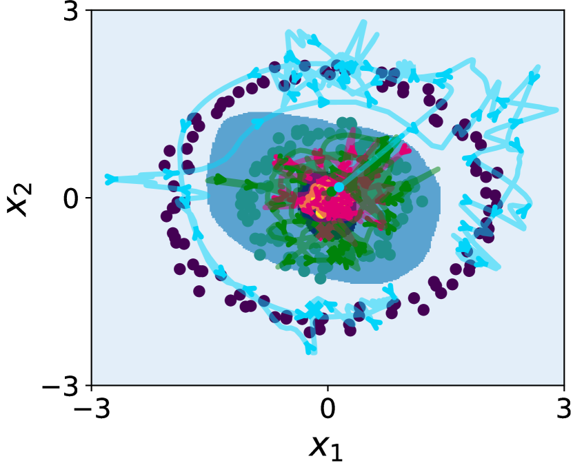
(b) Warm-start joint optimization.

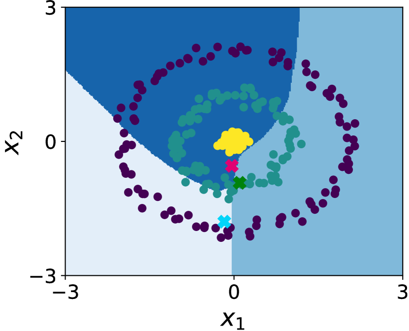
(c) Re-training on final points.

Figure 12: Dataset distillation fitting three classes with three learned datapoints. Similarly to the results in Sec. 4.1, when using warm-start joint optimization, the three learned datapoints adapt during training to trace out the data in their respective classes, guiding the network to learn a decision boundary that performs well on the original data. Cold-start re-training yields a model that correctly classifies the three learned datapoints, but has poor performance on the original data.

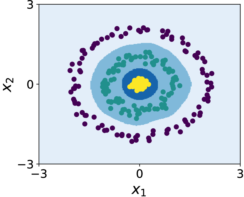
(a) Training on original data.

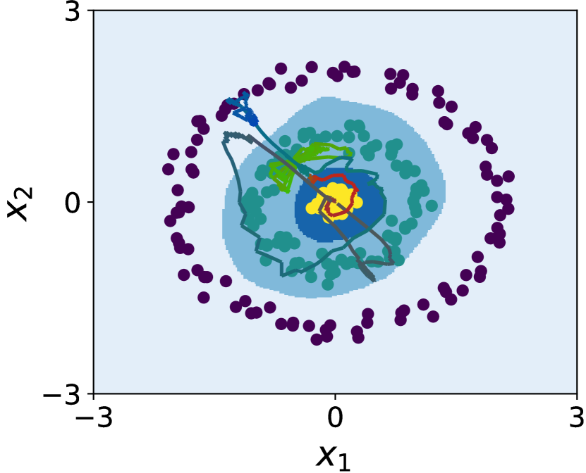
(b) Warm-start joint optimization.

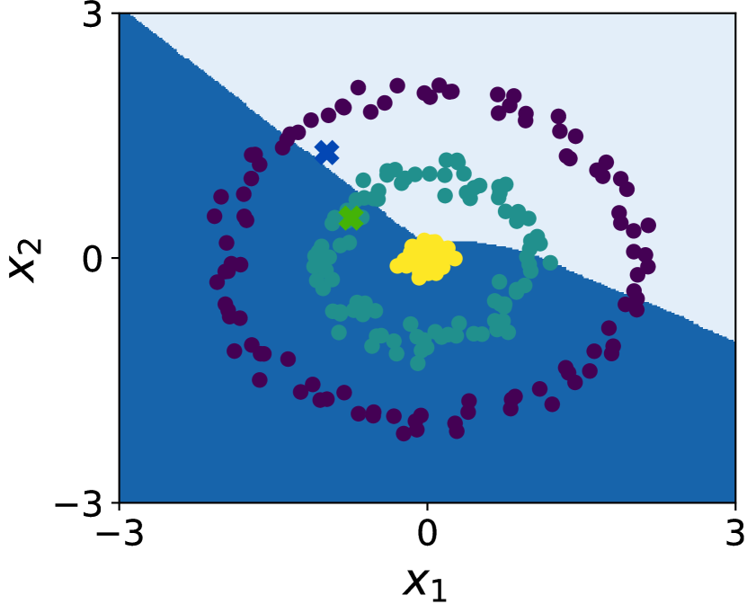
(c) Re-training on final points.

Figure 13: Dataset distillation results fitting three classes with only two learned datapoints. In the warm-start plot, the color of the trajectory of each learned datapoint indicates its soft class membership, with magenta, green, and blue corresponding to the inner, middle, and outer rings, respectively. Darker/gray colors indicate soft labels that place approximately equal probability on each class. We see that although we only have two learned datapoints, the class labels change over the course of training such that all three classes are covered. Cold-start re-training yields a model that correctly classifies the two learned datapoints, but has poor performance on the original data.

F.2 Details and Extended Results for Anti-Distillation

Details.

For the anti-distillation results in Section 4.2, we used a Fourier basis consisting of 10 $\sin$ terms, 10 $\cos$ terms, and a bias, yielding 21 total inner parameters. For the exponential-amplitude Fourier basis used in Section 4.2, we used SGD with learning rates 1e-7 and 1e-2 for the inner and outer parameters, respectively; for the $1/n$ amplitude Fourier basis (discussed below, and used for Figure 16), we used SGD with learning rates 1e-3 and 1e-2 for the inner and outer parameters, respectively.

Approximate Hypergradient Visualization.

For the visualization in Figure 11(c), the experiment setup is as follows: we have a single original dataset point at $(x,y)$ coordinate $(1,1)$, and we learn the $y$-coordinates of two synthetic datapoints, which we initialize at $(x,y)$-coordinates $(0,0)$ and $(2,0)$, respectively. The inner model trained on these two synthetic datapoints is a linear regressor with one weight and one bias, e.g., $y=wx+b$. The outer problem is overparameterized, because there are many valid settings of the learned datapoints such that the inner model trained on those datapoints will fit the point $(1,1)$. For example, three valid solutions for the learned datapoints are $\{(0,0),(2,2)\}$, $\{(0,1),(2,1)\}$, and $\{(0,2),(2,0)\}$. The set of such valid solutions is visualized in Figure 11(c), as well as the gradients using different hypergradient approximations, outer optimization trajectories, and converged outer solutions with each approximation. We focused on Neumann series approximations with different $k$, and ran the Neumann series at the converged inner parameters in each case.

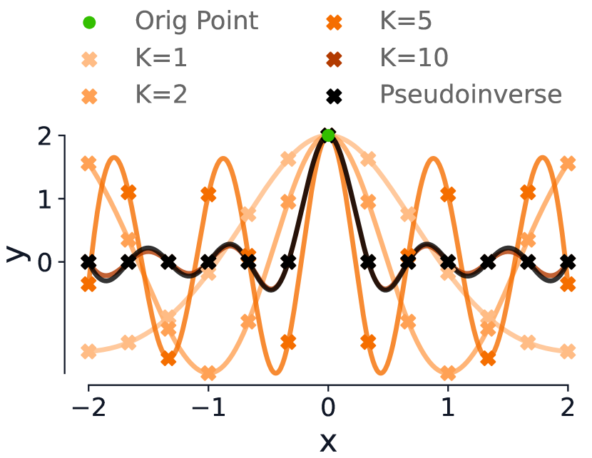
Figure 15: Truncated CG used to compute hypergradients for the anti-distillation task.

Conjugate Gradient.

Here, we present results using truncated conjugate gradient to approximate the inverse Hessian vector product when using the implicit function theorem to compute the hypergradient. We use the same problem setup as in Section 4.2, where we have a single validation datapoint and 13 learned datapoints. Because our Fourier basis consists of 10 $\sin$ terms, 10 $\cos$ terms, and a bias, we have 21 inner parameters, and using 21 steps of CG is guaranteed to yield the true inverse-Hessian vector product (barring any numerical issues). In Figure 15, we show the effect of using truncated CG iterations on the learned datapoints: we found that while Neumann iterations, truncated unrolling, and proximal optimization all yield nearly identical results, CG produces a very different inductive bias.

An Alternate Set of Fourier Basis Functions.

In Section 4.2, we used a Fourier basis in which the lower-frequency terms had exponentially larger amplitudes than the high-frequency terms. Figure 16 presents results using an alternative feature transform, where lower-frequency terms have linearly larger amplitudes than high-frequency terms.

$$\boldsymbol{\phi}(x)=\begin{bmatrix}1&\smash{\underbrace{\begin{matrix}\cos(x)&\frac{1}{2}\cos(2x)&\cdots&\frac{1}{L}\cos(Lx)\end{matrix}}_{L\cos\text{terms}}}&\smash{\underbrace{\begin{matrix}\sin(x)&\frac{1}{2}\sin(2x)&\cdots&\frac{1}{L}\sin(Lx)\end{matrix}}_{L\sin\text{terms}}}\end{bmatrix}$$

Thus, the inner problem aims to learn a weight vector $\mathbf{w}\in\mathbb{R}^{2N+1}$ that minimizes:

$$f(\mathbf{u},\mathbf{w})=\frac{1}{2}\|\mathbf{\Phi}\mathbf{w}-\mathbf{u}\|^{2}_{2}=\frac{1}{2}\sum_{i=1}^{n}\left(\mathbf{w}^{\top}\boldsymbol{\phi}(x_{i})-u_{i}\right)^{2}$$ (67)

where

$$\mathbf{w}^{\top}\boldsymbol{\phi}(x)=w_{0}+\sum_{\ell=1}^{L}\left(w_{\ell}\left(\frac{1}{\ell}\right)\cos(\ell x)+w_{L+\ell}\left(\frac{1}{\ell}\right)\sin(\ell x)\right)$$ (68)

(a) Neumann/unrolling

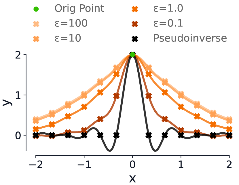
(b) Damped Hessian

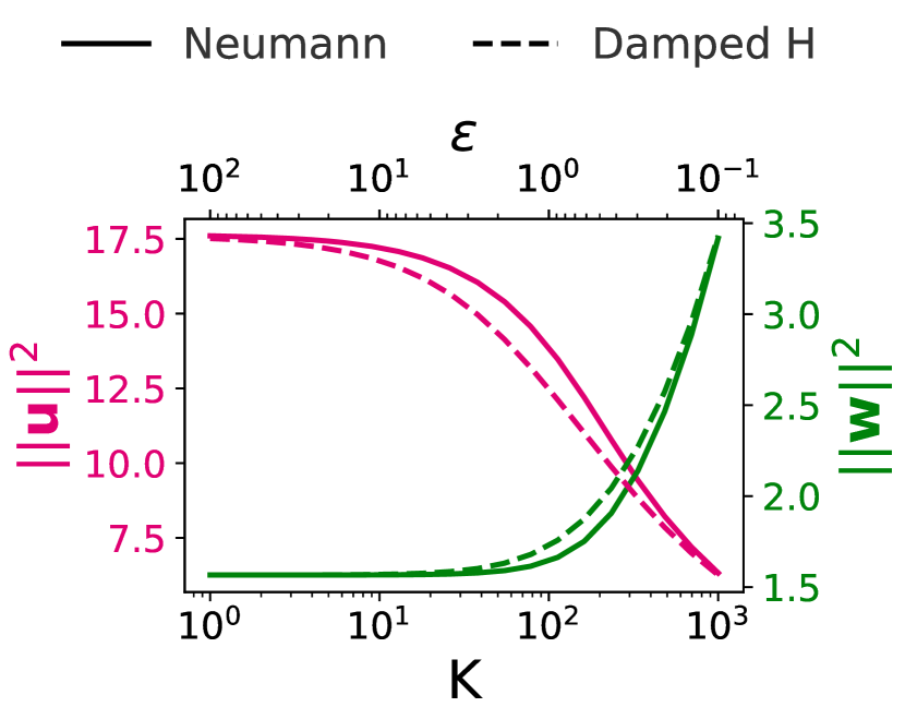
(c) Outer parameter norms.

Figure 16: Fourier-basis 1D linear regression, where the outer objective is overparameterized. We learn 13 synthetic datapoints such that a regressor trained on those points will fit a single original datapoint, shown by the green circle at $(0,2)$. The synthetic datapoints are initialized at linearly-spaced $x$-coordinates in the interval $[-2,2]$, with $y$-coordinate 0, and we only learn $y$ coordinates. In the Fourier basis we use, lower frequency components have larger amplitudes. Here, we use the $1/n$ amplitude scheme.

Underparameterized Inner Problem.

The antidistillation phenomena we describe occur in outer-overparameterized settings; they do not rely on inner overparameterization. In Figure 17, we show a version of experiment with an underparameterized inner problem (such that there is a unique inner optimum for each outer parameter, and the Hessian of the inner objective is invertible).

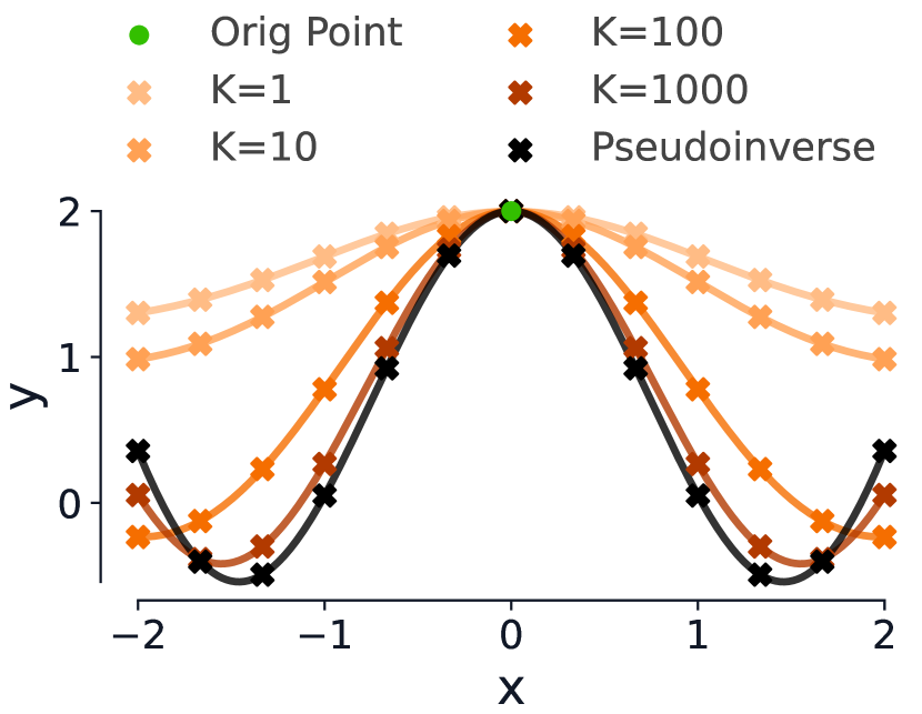
(a) Neumann/unrolling

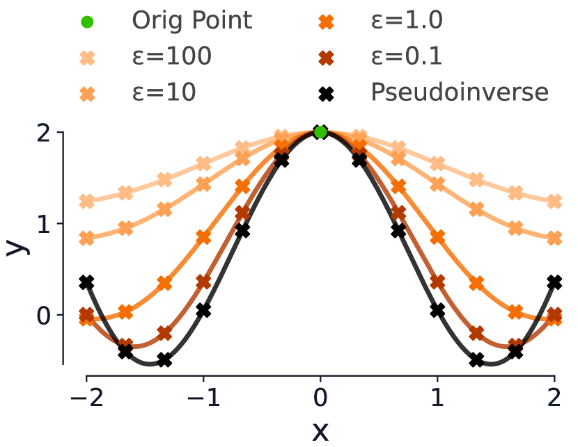
(b) Damped Hessian inverse

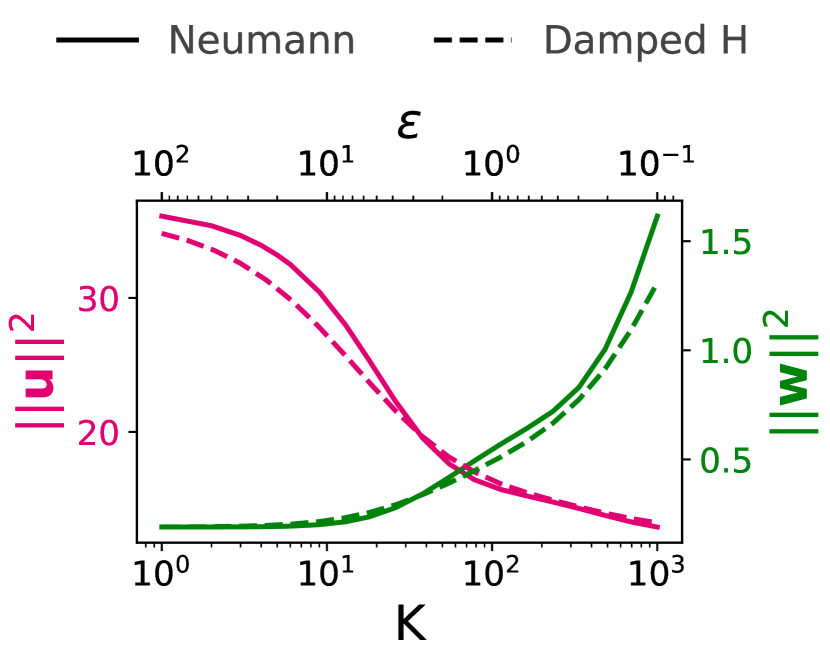
(c) Outer parameter norms.

Figure 17: Fourier-basis 1D linear regression, where the outer objective is overparameterized, but the inner objective is underparameterized. We learn 13 synthetic datapoints such that a regressor trained on those points will fit a single original datapoint, shown by the green circle at $(0,2)$. The synthetic datapoints are initialized at linearly-spaced $x$-coordinates in the interval $[-2,2]$, with $y$-coordinate 0, and we only learn the $y$-coordinates. In the Fourier basis we use, lower frequency components have larger amplitudes.

Using an MLP.

Finally, we show that similar conclusions hold when training a multi-layer perceptron (MLP) on the anti-distillation task. We used a 2-layer MLP with 10 hidden units per layer and ReLU activations. We used SGD with learning rate 0.01 for both the inner and outer parameters. Figure 18 shows the learned datapoints and model fits resulting from running several different steps of Neumann iterations or unrolling, as well as the norms of the inner and outer parameters as a function of $K$. For the Neumann experiments, we first optimize the MLP for 5000 steps to reach approximate convergence of the inner problem, before running $K$ Neumann iterations—the MLP is re-trained from scratch for 5000 steps for each outer parameter update (e.g., cold-started).

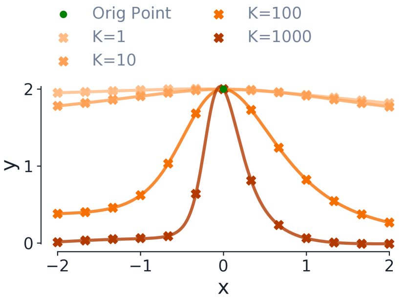
(a) Neumann

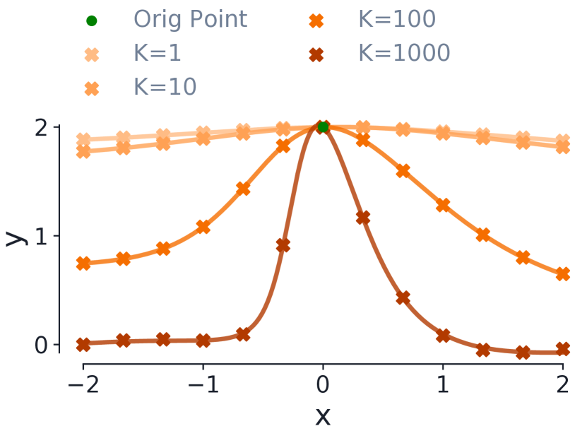
(b) Unrolling

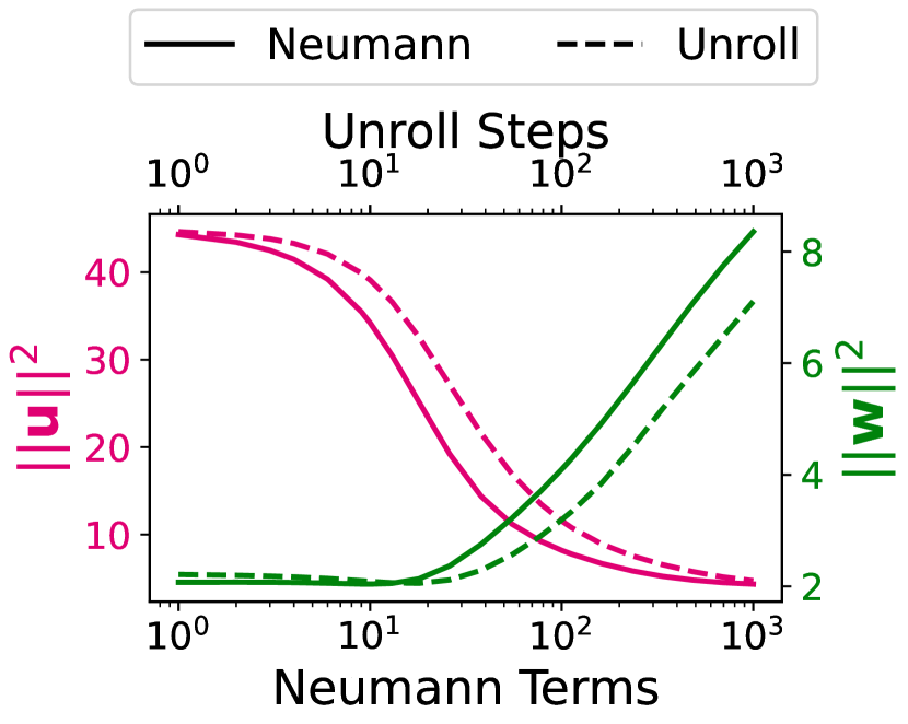
(c) Parameter norms.

Figure 18: 1D linear regression with an overparameterized outer objective, where we train an MLP rather than performing Fourier-basis function regression. Note that here we cannot analytically compute the damped Hessian inverse as in the linear regression case, so we only include results for full-unrolls with truncated Neumann approximations of the inverse Hessian, and alternating gradient descent with various numbers of unroll steps.

References

- Abadi et al. (2015) Abadi, M., Agarwal, A., Barham, P., Brevdo, E., Chen, Z., Citro, C., Corrado, G. S., Davis, A., Dean, J., Devin, M., Ghemawat, S., Goodfellow, I., Harp, A., Irving, G., Isard, M., Jia, Y., Jozefowicz, R., Kaiser, L., Kudlur, M., Levenberg, J., Mané, D., Monga, R., Moore, S., Murray, D., Olah, C., Schuster, M., Shlens, J., Steiner, B., Sutskever, I., Talwar, K., Tucker, P., Vanhoucke, V., Vasudevan, V., Viégas, F., Vinyals, O., Warden, P., Wattenberg, M., Wicke, M., Yu, Y., and Zheng, X. TensorFlow: Large-scale machine learning on heterogeneous systems, 2015. URL https://www.tensorflow.org/. Software available from tensorflow.org.
- Ali et al. (2019) Ali, A., Kolter, J. Z., and Tibshirani, R. J. A continuous-time view of early stopping for least squares regression. In International Conference on Artificial Intelligence and Statistics (AISTATS), pp. 1370–1378, 2019.
- Ali et al. (2020) Ali, A., Dobriban, E., and Tibshirani, R. The implicit regularization of stochastic gradient flow for least squares. In International Conference on Machine Learning (ICML), pp. 233–244, 2020.
- Amari et al. (2020) Amari, S.-i., Ba, J., Grosse, R., Li, X., Nitanda, A., Suzuki, T., Wu, D., and Xu, J. When does preconditioning help or hurt generalization? arXiv preprint arXiv:2006.10732, 2020.
- Angelos et al. (1998) Angelos, J., Grossman, G., Kaufman, E., Lenker, T., and Rakesh, L. Limit cycles for successive projections onto hyperplanes in RN. Linear Algebra and its Applications, 285(1-3):201–228, 1998.
- Arora et al. (2019) Arora, S., Du, S., Hu, W., Li, Z., and Wang, R. Fine-grained analysis of optimization and generalization for overparameterized two-layer neural networks. In International Conference on Machine Learning, pp. 322–332. PMLR, 2019.
- Bae & Grosse (2020) Bae, J. and Grosse, R. Delta-STN: Efficient bilevel optimization for neural networks using structured response Jacobians. Advances in Neural Information Processing Systems (NeurIPS), 2020.
- Bartlett et al. (2020) Bartlett, P. L., Long, P. M., Lugosi, G., and Tsigler, A. Benign overfitting in linear regression. Proceedings of the National Academy of Sciences, 117(48):30063–30070, 2020.
- Basri et al. (2020) Basri, R., Galun, M., Geifman, A., Jacobs, D., Kasten, Y., and Kritchman, S. Frequency bias in neural networks for input of non-uniform density. In International Conference on Machine Learning, pp. 685–694. PMLR, 2020.
- Belkin (2021) Belkin, M. Fit without fear: Remarkable mathematical phenomena of deep learning through the prism of interpolation. Acta Numerica, 30:203–248, 2021.
- Belkin et al. (2019) Belkin, M., Hsu, D., Ma, S., and Mandal, S. Reconciling modern machine-learning practice and the classical bias–variance trade-off. Proceedings of the National Academy of Sciences, 116(32):15849–15854, 2019.
- Bengio (2000) Bengio, Y. Gradient-based optimization of hyperparameters. Neural Computation, 12(8):1889–1900, 2000.
- Bengio et al. (2009) Bengio, Y., Louradour, J., Collobert, R., and Weston, J. Curriculum learning. In International Conference on Machine Learning (ICML), pp. 41–48, 2009.
- Blondel et al. (2021) Blondel, M., Berthet, Q., Cuturi, M., Frostig, R., Hoyer, S., Llinares-López, F., Pedregosa, F., and Vert, J.-P. Efficient and modular implicit differentiation. arXiv preprint arXiv:2105.15183, 2021.
- Bradbury et al. (2018) Bradbury, J., Frostig, R., Hawkins, P., Johnson, M. J., Leary, C., Maclaurin, D., Necula, G., Paszke, A., VanderPlas, J., Wanderman-Milne, S., and Zhang, Q. JAX: Composable transformations of Python+NumPy programs, 2018. URL http://github.com/google/jax.
- Chen & Hagan (1999) Chen, D. and Hagan, M. T. Optimal use of regularization and cross-validation in neural network modeling. In International Joint Conference on Neural Networks (IJCNN), volume 2, pp. 1275–1280, 1999.
- Dempe (2002) Dempe, S. Foundations of bilevel programming. Springer Science & Business Media, 2002.
- Dempe et al. (2007) Dempe, S., Dutta, J., and Mordukhovich, B. New necessary optimality conditions in optimistic bilevel programming. Optimization, 56(5-6):577–604, 2007.
- Dempe et al. (2014) Dempe, S., Mordukhovich, B. S., and Zemkoho, A. B. Necessary optimality conditions in pessimistic bilevel programming. Optimization, 63(4):505–533, 2014.
- Domke (2012) Domke, J. Generic methods for optimization-based modeling. In Artificial Intelligence and Statistics, pp. 318–326, 2012.
- Finn et al. (2017) Finn, C., Abbeel, P., and Levine, S. Model-agnostic meta-learning for fast adaptation of deep networks. In International Conference on Machine Learning (ICML), pp. 1126–1135, 2017.
- Foo et al. (2008) Foo, C.-s., Do, C. B., and Ng, A. Y. Efficient multiple hyperparameter learning for log-linear models. In Advances in Neural Information Processing Systems (NeurIPS), pp. 377–384, 2008.
- Franceschi et al. (2018) Franceschi, L., Frasconi, P., Salzo, S., Grazzi, R., and Pontil, M. Bilevel programming for hyperparameter optimization and meta-learning. arXiv preprint arXiv:1806.04910, 2018.
- Friedman & Popescu (2003) Friedman, J. and Popescu, B. E. Gradient directed regularization for linear regression and classification. Technical report, Statistics Department, Stanford University, 2003.
- Gerfo et al. (2008) Gerfo, L. L., Rosasco, L., Odone, F., Vito, E. D., and Verri, A. Spectral algorithms for supervised learning. Neural Computation, 20(7):1873–1897, 2008.
- Ghadimi & Wang (2018) Ghadimi, S. and Wang, M. Approximation methods for bilevel programming. arXiv preprint arXiv:1802.02246, 2018.
- Goodfellow et al. (2014) Goodfellow, I. J., Pouget-Abadie, J., Mirza, M., Xu, B., Warde-Farley, D., Ozair, S., Courville, A., and Bengio, Y. Generative adversarial networks. In Advances in Neural Information Processing Systems (NeurIPS), 2014.
- Grazzi et al. (2020a) Grazzi, R., Franceschi, L., Pontil, M., and Salzo, S. On the iteration complexity of hypergradient computation. In International Conference on Machine Learning (ICML), pp. 3748–3758, 2020a.
- Grazzi et al. (2020b) Grazzi, R., Pontil, M., and Salzo, S. Convergence properties of stochastic hypergradients. arXiv preprint arXiv:2011.07122, 2020b.
- Gunasekar et al. (2018) Gunasekar, S., Lee, J., Soudry, D., and Srebro, N. Characterizing implicit bias in terms of optimization geometry. In International Conference on Machine Learning (ICML), pp. 1832–1841, 2018.
- Ha et al. (2017) Ha, D., Dai, A., and Le, Q. V. Hypernetworks. In International Conference on Learning Representations (ICLR), 2017.
- Harker & Pang (1988) Harker, P. T. and Pang, J.-S. Existence of optimal solutions to mathematical programs with equilibrium constraints. Operations Research Letters, 7(2):61–64, 1988.
- Hataya et al. (2020a) Hataya, R., Zdenek, J., Yoshizoe, K., and Nakayama, H. Faster Autoaugment: Learning augmentation strategies using backpropagation. In European Conference on Computer Vision (ECCV), pp. 1–16, 2020a.
- Hataya et al. (2020b) Hataya, R., Zdenek, J., Yoshizoe, K., and Nakayama, H. Meta approach to data augmentation optimization. arXiv preprint arXiv:2006.07965, 2020b.
- Ho et al. (2019) Ho, D., Liang, E., Chen, X., Stoica, I., and Abbeel, P. Population based augmentation: Efficient learning of augmentation policy schedules. In International Conference on Machine Learning (ICML), pp. 2731–2741, 2019.
- Hong et al. (2020) Hong, M., Wai, H.-T., Wang, Z., and Yang, Z. A two-timescale framework for bilevel optimization: Complexity analysis and application to actor-critic. arXiv preprint arXiv:2007.05170, 2020.
- Jacot et al. (2018) Jacot, A., Gabriel, F., and Hongler, C. Neural tangent kernel: Convergence and generalization in neural networks. In Advances in Neural Information Processing Systems (NeurIPS), 2018.
- Jaderberg et al. (2017) Jaderberg, M., Dalibard, V., Osindero, S., Czarnecki, W. M., Donahue, J., Razavi, A., Vinyals, O., Green, T., Dunning, I., Simonyan, K., et al. Population based training of neural networks. arXiv preprint arXiv:1711.09846, 2017.
- Ji & Liang (2021) Ji, K. and Liang, Y. Lower bounds and accelerated algorithms for bilevel optimization. arXiv preprint arXiv:2102.03926, 2021.
- Ji et al. (2020) Ji, K., Yang, J., and Liang, Y. Bilevel optimization: Nonasymptotic analysis and faster algorithms. arXiv preprint arXiv:2010.07962, 2020.
- Ji et al. (2021) Ji, K., Yang, J., and Liang, Y. Bilevel optimization: Convergence analysis and enhanced design. In International Conference on Machine Learning (ICML), pp. 4882–4892, 2021.
- Ji & Telgarsky (2019) Ji, Z. and Telgarsky, M. The implicit bias of gradient descent on nonseparable data. In Conference on Learning Theory, pp. 1772–1798, 2019.
- Karczmarz (1937) Karczmarz, S. Angenaherte Auflosung von Systemen linearer Gleichungen. Bull. Int. Acad. Pol. Sic. Let., Cl. Sci. Math. Nat., pp. 355–357, 1937.
- Koh & Liang (2017) Koh, P. W. and Liang, P. Understanding black-box predictions via influence functions. In International Conference on Machine Learning (ICML), pp. 1885–1894, 2017.
- Larsen et al. (1996) Larsen, J., Hansen, L. K., Svarer, C., and Ohlsson, M. Design and regularization of neural networks: The optimal use of a validation set. In IEEE Signal Processing Society Workshop, pp. 62–71, 1996.
- Lee et al. (2019) Lee, J., Xiao, L., Schoenholz, S. S., Bahri, Y., Novak, R., Sohl-Dickstein, J., and Pennington, J. Wide neural networks of any depth evolve as linear models under gradient descent. In Advances in Neural Information Processing Systems (NeurIPS), 2019.
- Liao et al. (2018) Liao, R., Xiong, Y., Fetaya, E., Zhang, L., Yoon, K., Pitkow, X., Urtasun, R., and Zemel, R. Reviving and improving recurrent back-propagation. In International Conference on Machine Learning (ICML), 2018.
- Lignola & Morgan (1995) Lignola, M. B. and Morgan, J. Topological existence and stability for Stackelberg problems. Journal of Optimization Theory and Applications, 84(1):145–169, 1995.
- Lignola & Morgan (2001) Lignola, M. B. and Morgan, J. Existence of solutions to bilevel variational problems in Banach spaces. In Equilibrium Problems: Nonsmooth Optimization and Variational Inequality Models, pp. 161–174. Springer, 2001.
- Liu et al. (2019) Liu, H., Simonyan, K., and Yang, Y. DARTS: Differentiable architecture search. In International Conference on Learning Representations (ICLR), 2019.
- Liu et al. (2018) Liu, J., Fan, Y., Chen, Z., and Zheng, Y. Pessimistic bilevel optimization: A survey. International Journal of Computational Intelligence Systems, 11(1):725–736, 2018.
- Liu et al. (2020) Liu, J., Fan, Y., Chen, Z., and Zheng, Y. Methods for pessimistic bilevel optimization. In Bilevel Optimization, pp. 403–420. Springer, 2020.
- Loridan & Morgan (1996) Loridan, P. and Morgan, J. Weak via strong Stackelberg problem: New results. Journal of Global Optimization, 8(3):263–287, 1996.
- Lorraine & Duvenaud (2017) Lorraine, J. and Duvenaud, D. Stochastic hyperparameter optimization through hypernetworks. In NIPS Meta-Learning Workshop, 2017.
- Lorraine et al. (2020) Lorraine, J., Vicol, P., and Duvenaud, D. Optimizing millions of hyperparameters by implicit differentiation. In International Conference on Artificial Intelligence and Statistics (AISTATS), pp. 1540–1552, 2020.
- Lucchetti et al. (1987) Lucchetti, R., Mignanego, F., and Pieri, G. Existence theorems of equilibrium points in Stackelberg games with constraints. Optimization, 18(6):857–866, 1987.
- Luketina et al. (2016) Luketina, J., Berglund, M., Greff, K., and Raiko, T. Scalable gradient-based tuning of continuous regularization hyperparameters. In International Conference on Machine Learning (ICML), pp. 2952–2960, 2016.
- MacKay et al. (2019) MacKay, M., Vicol, P., Lorraine, J., Duvenaud, D., and Grosse, R. Self-Tuning Networks: Bilevel optimization of hyperparameters using structured best-response functions. In International Conference on Learning Representations (ICLR), 2019.
- Maclaurin et al. (2015) Maclaurin, D., Duvenaud, D., and Adams, R. Gradient-based hyperparameter optimization through reversible learning. In International Conference on Machine Learning (ICML), pp. 2113–2122, 2015.
- Mehra & Hamm (2019) Mehra, A. and Hamm, J. Penalty method for inversion-free deep bilevel optimization. arXiv preprint arXiv:1911.03432, 2019.
- Metz et al. (2019) Metz, L., Maheswaranathan, N., Nixon, J., Freeman, D., and Sohl-Dickstein, J. Understanding and correcting pathologies in the training of learned optimizers. In International Conference on Machine Learning (ICML), pp. 4556–4565, 2019.
- Micaelli & Storkey (2020) Micaelli, P. and Storkey, A. Non-greedy gradient-based hyperparameter optimization over long horizons. arXiv preprint arXiv:2007.07869, 2020.
- Mishachev & Shmyrin (2019) Mishachev, N. and Shmyrin, A. M. On realization of limit polygons in sequential projection method. International Transaction Journal of Engineering, Management and Applied Sciences and Technologies, 10(15):1015–1015, 2019.
- Morgan & Bourlard (1989) Morgan, N. and Bourlard, H. Generalization and parameter estimation in feedforward nets: Some experiments. Advances in Neural Information Processing Systems (NeurIPS), 2:630–637, 1989.
- Mounsaveng et al. (2021) Mounsaveng, S., Laradji, I., Ben Ayed, I., Vazquez, D., and Pedersoli, M. Learning data augmentation with online bilevel optimization for image classification. In Winter Conference on Applications of Computer Vision, pp. 1691–1700, 2021.
- Nacson et al. (2019) Nacson, M. S., Srebro, N., and Soudry, D. Stochastic gradient descent on separable data: Exact convergence with a fixed learning rate. In International Conference on Artificial Intelligence and Statistics (AISTATS), pp. 3051–3059, 2019.
- Nakkiran et al. (2020) Nakkiran, P., Kaplun, G., Bansal, Y., Yang, T., Barak, B., and Sutskever, I. Deep double descent: Where bigger models and more data hurt. In International Conference on Learning Representations (ICLR), 2020.
- Outrata (1993) Outrata, J. V. Necessary optimality conditions for Stackelberg problems. Journal of Optimization Theory and Applications, 76(2):305–320, 1993.
- Paszke et al. (2017) Paszke, A., Gross, S., Chintala, S., Chanan, G., Yang, E., DeVito, Z., Lin, Z., Desmaison, A., Antiga, L., and Lerer, A. Automatic differentiation in PyTorch. In NIPS Workshop Autodifferentiation, 2017.
- Pearlmutter (1994) Pearlmutter, B. A. Fast exact multiplication by the Hessian. Neural Computation, 6(1):147–160, 1994.
- Pedregosa (2016) Pedregosa, F. Hyperparameter optimization with approximate gradient. In International Conference on Machine Learning (ICML), 2016.
- Peng et al. (2018) Peng, X., Tang, Z., Yang, F., Feris, R. S., and Metaxas, D. Jointly optimize data augmentation and network training: Adversarial data augmentation in human pose estimation. In Conference on Computer Vision and Pattern Recognition (CVPR), pp. 2226–2234, 2018.
- Pfau & Vinyals (2016) Pfau, D. and Vinyals, O. Connecting generative adversarial networks and actor-critic methods. In NeurIPS Workshop on Adversarial Training, 2016.
- Poggio et al. (2019) Poggio, T., Banburski, A., and Liao, Q. Theoretical issues in deep networks: Approximation, optimization and generalization. In Proceedings of the National Academy of Sciences, 2019.
- Raghu et al. (2020) Raghu, A., Raghu, M., Kornblith, S., Duvenaud, D., and Hinton, G. Teaching with commentaries. In International Conference on Learning Representations (ICLR), 2020.
- Rahaman et al. (2019) Rahaman, N., Baratin, A., Arpit, D., Draxler, F., Lin, M., Hamprecht, F., Bengio, Y., and Courville, A. On the spectral bias of neural networks. In International Conference on Machine Learning, pp. 5301–5310. PMLR, 2019.
- Rajeswaran et al. (2019) Rajeswaran, A., Finn, C., Kakade, S., and Levine, S. Meta-learning with implicit gradients. In Advances in Neural Information Processing Systems (NeurIPS), 2019.
- Ren et al. (2018) Ren, M., Zeng, W., Yang, B., and Urtasun, R. Learning to reweight examples for robust deep learning. In International Conference on Machine Learning (ICML), pp. 4334–4343, 2018.
- Rosasco (2009) Rosasco, L. 9.520: Statistical Learning Theory and Applications, Lecture 7. Lecture Notes, 2009. URL https://www.mit.edu/~9.520/spring09/Classes/class07_spectral.pdf.
- Shaban et al. (2019) Shaban, A., Cheng, C.-A., Hatch, N., and Boots, B. Truncated back-propagation for bilevel optimization. In International Conference on Artificial Intelligence and Statistics (AISTATS), pp. 1723–1732, 2019.
- Sinha et al. (2017) Sinha, A., Malo, P., and Deb, K. A review on bilevel optimization: From classical to evolutionary approaches and applications. IEEE Transactions on Evolutionary Computation, 22(2):276–295, 2017.
- Sohl-Dickstein et al. (2020) Sohl-Dickstein, J., Novak, R., Schoenholz, S. S., and Lee, J. On the infinite width limit of neural networks with a standard parameterization. arXiv preprint arXiv:2001.07301, 2020.
- Soudry et al. (2018) Soudry, D., Hoffer, E., Nacson, M. S., Gunasekar, S., and Srebro, N. The implicit bias of gradient descent on separable data. The Journal of Machine Learning Research, 19(1):2822–2878, 2018.
- Stošić et al. (2016) Stošić, M., Xavier, J., and Dodig, M. Projection on the intersection of convex sets. Linear Algebra and its Applications, 509:191–205, 2016.
- Strand (1974) Strand, O. N. Theory and methods related to the singular-function expansion and Landweber’s iteration for integral equations of the first kind. SIAM Journal on Numerical Analysis, 11(4):798–825, 1974.
- Suggala et al. (2018) Suggala, A., Prasad, A., and Ravikumar, P. K. Connecting optimization and regularization paths. Advances in Neural Information Processing Systems (NeurIPS), 31:10608–10619, 2018.
- Tancik et al. (2020) Tancik, M., Srinivasan, P., Mildenhall, B., Fridovich-Keil, S., Raghavan, N., Singhal, U., Ramamoorthi, R., Barron, J., and Ng, R. Fourier features let networks learn high frequency functions in low dimensional domains. Advances in Neural Information Processing Systems, 33:7537–7547, 2020.
- Tang et al. (2020) Tang, Z., Gao, Y., Karlinsky, L., Sattigeri, P., Feris, R., and Metaxas, D. OnlineAugment: Online data augmentation with less domain knowledge. In European Conference on Computer Vision (ECCV), 2020.
- Vardi & Shamir (2021) Vardi, G. and Shamir, O. Implicit regularization in ReLU networks with the square loss. In Conference on Learning Theory, pp. 4224–4258, 2021.
- Wang et al. (2018) Wang, T., Zhu, J.-Y., Torralba, A., and Efros, A. A. Dataset distillation. arXiv preprint arXiv:1811.10959, 2018.
- Wiesemann et al. (2013) Wiesemann, W., Tsoukalas, A., Kleniati, P.-M., and Rustem, B. Pessimistic bilevel optimization. SIAM Journal on Optimization, 23(1):353–380, 2013.
- Wu & Xu (2020) Wu, D. and Xu, J. On the optimal weighted regularization in overparameterized linear regression. arXiv preprint arXiv:2006.05800, 2020.
- Wu et al. (2018) Wu, Y., Ren, M., Liao, R., and Grosse, R. Understanding short-horizon bias in stochastic meta-optimization. In International Conference on Learning Representations (ICLR), 2018.
- Yang et al. (2021) Yang, J., Ji, K., and Liang, Y. Provably faster algorithms for bilevel optimization. arXiv preprint arXiv:2106.04692, 2021.
- Yao et al. (2007) Yao, Y., Rosasco, L., and Caponnetto, A. On early stopping in gradient descent learning. Constructive Approximation, 26(2):289–315, 2007.
- Zhang et al. (2016) Zhang, C., Bengio, S., Hardt, M., Recht, B., and Vinyals, O. Understanding deep learning requires rethinking generalization. In International Conference on Learning Representations (ICLR), 2016.
- Zhao et al. (2021) Zhao, B., Mopuri, K. R., and Bilen, H. Dataset condensation with gradient matching. In International Conference on Learning Representations (ICLR), 2021.
- Zoph & Le (2017) Zoph, B. and Le, Q. V. Neural architecture search with reinforcement learning. In International Conference on Learning Representations (ICLR), 2017.