Non-Gaussian fluctuation dynamics in relativistic fluids

Abstract

We consider non-equilibrium evolution of non-Gaussian fluctuations within relativistic hydrodynamics relevant for the QCD critical point search in heavy-ion collision experiments. We rely on the hierarchy of relaxation time scales, which emerges in the hydrodynamic regime near the critical point, to focus on the slowest mode such as the fluctuations of specific entropy, whose equilibrium magnitude, non-Gaussianity and typical relaxation time are increasing as the critical point is approached. We derive evolution equations for the non-Gaussian correlators of this diffusive mode in an arbitrary relativistic hydrodynamic flow. We compare with the simpler case of the stochastic diffusion on a static homogeneous background and identify terms which are specific to the case of the full hydrodynamics with pressure fluctuations and flow.

I Introduction

The physics of thermal fluctuations Landau:2013stat2 in hydrodynamics Landau:2013fluid has received renewed interest recently in the context of relativistic heavy-ion collision experiments. Hydrodynamics proved to be remarkably successful in describing the data from such collisions Jeon:2015dfa ; Romatschke:2017ejr . One of the major goals of heavy-ion collision experiments is the discovery of the QCD critical point – the end point of the conjectured first-order transition separating hadron gas and the quark-gluon plasma phases Aggarwal:2010cw . This point is characterized by a certain singular behavior of fluctuations – a universal feature of the critical points Stephanov:1998dy ; Stephanov:1999zu ; Stephanov:2004wx . Therefore, understanding of fluctuations and, in particular, of their non-equilibrium evolution in the environment of the hydrodynamically expanding QCD fireball is important to enable the experimental search for the QCD critical point Bzdak:2019pkr ; An_2022 .

The parameter controlling the importance of fluctuations at wavelengths of order $\ell$ is the ratio of the “correlation volume” of the size of the correlation length $\xi$ to the “homogeneity volume” of order $\ell^{3}$. We shall generically refer to this parameter as $\varepsilon$. The central limit theorem suppresses the magnitude of fluctuations as well as their non-Gaussianity by a power of $\varepsilon$. In a typical condensed matter experiment $\varepsilon$ is extremely small and thus fluctuations often play a negligible role. In heavy-ion collisions, where the system size ($\mathcal{O}(10\text{ fm})$) is large compared to the typical correlation length $\xi$ (a fraction of fm), the parameter $\varepsilon$ is small but not negligible. Fluctuations are observable in heavy-ion collisions and play important role in understanding the thermodynamic properties of the QCD fireball.

Furthermore, near the critical point, as the correlation length becomes longer, the fluctuations grow and play even more important role. Non-Gaussianity of fluctuations, also controlled by $\varepsilon$, is increasing even faster at the critical point than their magnitude Stephanov:2008qz , and is expected to show a specific nonmonotonic dependence on the collision energy Stephanov:2011pb , which in heavy-ion collisions controls the thermodynamic conditions at freeze-out. Therefore, non-Gaussian fluctuation measures have emerged as observables of primary experimental interest in the search for the QCD critical point STAR:2021iop .

Another effect of the critical point is to slow down the relaxation towards local thermodynamic equilibrium. The critical slowing down makes it increasingly important to consider non-equilibrium evolution of fluctuations near the critical point, as earlier estimates and model calculations demonstrate Stephanov:1999zu ; Berdnikov:1999ph ; Mukherjee:2015swa . To make quantitatively reliable predictions, however, one needs to consider the non-equilibrium behavior of fluctuations in the “first principle” hydrodynamic approach.

There has been considerable recent effort and progress towards understanding non-equilibrium evolution of fluctuations in the context of the hydrodynamics of the heavy-ion collisions with the aim of mapping the QCD phase diagram (see Ref. An_2022 and references therein). The focus of this paper is on the approach where fluctuations are described in terms of the correlation functions obeying deterministic evolution equations, i.e., the so-called deterministic (also known as hydrokinetic) approach. This approach was introduced and developed recently in the context of relativistic heavy-ion collisions Akamatsu:2017 ; Akamatsu:2018 ; Martinez:2018 , more generally in An:2019rhf ; An:2019fdc ; An:2020jjk ; An_2021 ; An:2022tfk , and much earlier, in the non-relativistic condensed matter context, in andreev1970twoliquid ; Andreev:1978 .

Within the deterministic approach most of the work has been done on Gaussian fluctuation measures: two-point correlators, or their Wigner transforms. In this approach, the first step towards the study of the non-Gaussian hydrodynamic fluctuations out of equilibrium was made in Ref. An_2021 , where the generalized $n$-point Wigner transform was introduced and the equations for the corresponding $n$-point Wigner functions were derived. Ref. An_2021 considered the simplest hydrodynamic system: nonlinear charge diffusion at constant temperature. Such a system is characterized by a single hydrodynamic field: conserved charge density. Full hydrodynamics necessary to describe heavy-ion collisions involves (at least) five hydrodynamic fields: conserved densities of energy, baryon charge and three-momentum of the fluid. The full theory of hydrodynamic fluctuations is an ambitious goal and in this paper we shall present another step towards it by considering fluctuations of both energy and baryon density in the regime relevant to the critical point search, where the correlation length becomes large compared to typical microscopic scales (while still being smaller than $\ell$) and fluctuations of a certain critical mode dominate.

In this regime an important hierarchy of scales emerges. The slowest mode is the diffusive (nonpropagating) mode $m=s/n$, i.e., entropy to baryon number ratio, which we shall refer to as specific entropy. This mode does not mix with propagating sound oscillations, which makes it purely diffusive (unlike fluctuations of energy and baryon densities on their own). Furthermore, unlike the case of other diffusive modes, such as transverse momentum densities, the diffusion constant for $m$ vanishes at the critical point making $m$ the slowest mode in this regime. Such a hierarchy of scales was exploited in the construction of Hydro+ theory in Ref. Stephanov:2018hydro+ as well as in the Hydro++ theory in Ref. An:2019fdc , where the next-to-slowest momentum diffusion modes were also included. In both cases only two-point correlators were considered. The goal of this work is to extend the Hydro+ formalism to the non-Gaussian fluctuation measures, i.e., $n$-point correlation functions.

As in Ref. Stephanov:2018hydro+ we shall focus on fluctuations of $m$, which are important for two related reasons. First, as explained above, this mode and its fluctuations are slowest to relax, and therefore are most in need of nonequilibrium description. Second, the magnitude and non-Gaussianity measures of the fluctuations of this mode diverge with the correlation length most strongly (with the largest critical exponent), thus providing the most sensitive observable signatures of the critical point.

Furthermore, in Ref. An_2021 we considered fluctuations in a stationary fluid without any flow. Here we shall treat the most general relativistic flow in a fully Lorentz covariant formalism necessary for applications to heavy-ion collisions. We review the formalism which was introduced in Ref. An:2019rhf ; An:2019fdc for two-point correlators with a specific focus on generalizing it to non-Gaussian fluctuations. We use the $n$-point wave number dependent correlation functions which we introduced in Ref. An_2021 by generalizing the well-known Wigner transform and show how the confluent formalism of Refs. An:2019rhf ; An:2019fdc naturally extends to these objects in Section II.4.

While the simple diffusion problem in Ref. An_2021 contains only one fluctuating field variable (charge density $n$), we find that—even in the regime where the fluctuations of $m$ are the slowest and the fluctuations of the faster hydrodynamic modes, such as pressure $p$, can be considered as equilibrated—we cannot neglect these fluctuations, as they modify equations for the evolution of fluctuations of $m$ via nonlinearities in the equation of state, or mode coupling. We discuss this nontrivial part of the derivation in Section III.2.

We should point out again that we set up the formalism in the most general form necessary to tackle the full system of hydrodynamic equations with fluctuations of all hydrodynamic variables. Our focus on the slowest variable $m$ allows us to make the logical first step towards considering the full system. This focus simplifies the calculations and allows us to hone the tools needed to tackle this ambitious goal.

We shall use the approach of Refs. An:2019rhf ; An:2019fdc , i.e., expand the stochastic hydrodynamic equations in powers of fluctuation magnitude. Unlike Refs. An:2019rhf ; An:2019fdc we shall not consider feedback of fluctuations and assume, based on the analysis of these contributions in Refs. An:2019rhf ; An:2019fdc , that the major effect of these (UV sensitive) contributions have been absorbed into renormalization of hydrodynamic variables, equation of state and transport coefficients which, therefore, take physical (cutoff independent) values. In the diagrammatic representation we introduced in Ref. An_2021 such feedback contributions are represented by loop diagrams. As in Ref. An_2021 , we shall consider only “tree-level” terms in the evolution equations for non-Gaussian correlators. Again, this is not a limitation of the approach, but a natural simplifying first step in its development.

In Sec. II we introduce the general formalism for the dynamical evolution equations for the $n$-point correlation functions in the presence of background hydrodynamic flow. In Sec. III we focus on the specific entropy fluctuations for reasons explained above and, by using the results developed in Sec. II, we derive the evolution equations for the two-, three- and four-point functions of the specific entropy fluctuations. Thus we arrive at the main results of this paper which can be found in Sec. III.2. We summarize our findings and discuss the outlook for future developments in Sec. IV.

II General deterministic formalism for field fluctuations

In this section we extend the formalism for the dynamical evolution equation of relativistic hydrodynamic fluctuations we developed in Refs. An:2019rhf ; An:2019fdc to $n$-point correlation functions. In particular, we show that the confluent formalism, which allows us to describe fluctuations in the local rest frame of the fluid in a natural and fully Lorentz covariant way, generalizes naturally to $n$-point functions. We also use the multipoint Wigner transform, which we introduced in Ref. An_2021 , to express the $n$-point correlators in terms of one spatial coordinate of the midpoint and $n-1$ independent wave vectors. The results of this section are general, i.e., not limited to a particular fluctuating variable of variables.

II.1 Evolution of correlation functions

Let us first derive the evolution equation for the $n$-point correlation functions of a set of generic stochastic field variables $\breve{\psi}_{i}$ where the subscript $i$ labels different local hydrodynamic fields (such as entropy per baryon $m\equiv s/n$, pressure $p$, and fluid velocity $u$ as in Refs. An:2019rhf ; An:2019fdc ). Each of those variables satisfies its own Langevin-type equation that can be generically written in a covariant form,

$$\breve{u}\cdot\partial\breve{\psi}_{i}=\breve{F}_{i}+\xi_{i}\,,\quad\mbox{with}\quad\xi_{i}=\breve{H}_{ij}\eta_{j}\,,$$ (1)

where the symbol “$~{}\breve{~{}}~{}$” denotes a stochastic quantity. Functions or functionals, such as $\breve{u}\equiv u(\breve{\psi}_{i})$ or $\breve{F}\equiv F(\breve{\psi})$ inherit the stochastic symbol “$~{}\breve{~{}}~{}$” from their arguments. The four-velocity obeys $\breve{u}^{2}=-1$, and should be understood as a four-vector function of $\psi_{i}$’s (or can also be chosen to be among the variables $\psi_{i}$ as in Refs. An:2019rhf ; An:2019fdc ). $\breve{F}_{i}$ is the drift “force” and $\xi_{i}$ is the noise (random “force”) for the variable $\psi_{i}$, expressed in terms of the canonically normalized local Gaussian noise:

$$\langle{\eta_{i}}\rangle=0\,,\qquad\langle{\eta_{i}(x_{1})\eta_{j}(x_{2})}\rangle=2\delta_{ij}\delta^{(4)}(x_{1}-x_{2})\,.$$ (2)

We include multiplicative noise, since $\breve{H}=H(\breve{\psi})$, and define the product $\breve{H}\eta$ in terms of the It${\bar{\rm o}}$ calculus.

The Onsager matrix (operator) $Q=Q^{T}$ is the “square” of $H$: $Q_{ij}\equiv H_{ik}H_{jk}$.

Denoting fluctuation of a given stochastic quantity $\breve{X}$ as

$$\,:\!\breve{X}\!:\,\equiv\delta X\equiv\breve{X}-\langle\breve{X}\rangle\equiv\breve{X}-X\,,$$ (3)

and introducing the fluctuation of the variables $\psi_{i}$,

$$\phi_{i}\equiv\,:\!{\breve{\psi}}_{i}\!:\,\equiv{\breve{\psi}}_{i}-\psi_{i}\,,$$ (4)

we can expand the stochastic equations (1) in powers of $\phi_{i}$, using, e.g.,

$$\breve{F}_{i}=\sum_{n=0}^{\infty}\frac{1}{n!}F_{i,\,j_{1}\dots j_{n}}\phi_{j_{1}}\dots\phi_{j_{n}}=F_{i}+F_{i,\,j_{1}}\phi_{j_{1}}+\frac{1}{2}F_{i,\,j_{1}j_{2}}\phi_{j_{1}}\phi_{j_{2}}+\dots\,,$$ (5)

where $F\equiv F(\psi)$, etc. , and obtain the evolution equation for fluctuation field $\phi_{i}$:

$$u\cdot\partial\phi_{i}=\,:\!\breve{u}\cdot\partial{\breve{\psi}}_{i}-\delta u\cdot\partial{\breve{\psi}}_{i}:\,\,= :\sum_{n=1}^{\infty}\frac{1}{n!}L_{i,\,j_{1}\dots j_{n}}\phi_{j_{1}}\dots\phi_{j_{n}}+\xi_{i}\!:\,\,,$$ (6)

where the term involving $\delta u$ in Eq. (6) must be kept if the fluctuation of velocity is taken into account and

$$L_{i,\,j_{1}j_{2}\dots j_{n}}=F_{i,\,j_{1}j_{2}\dots j_{n}}-u^{\mu}_{,\,j_{1}\dots j_{n}}(\partial_{\mu}\psi_{i})-\left[n\delta_{ij_{1}}u^{\mu}_{,\,j_{2}\dots j_{n}}\partial_{\mu}^{(j_{1})}\right]_{\overline{1\dots n}}\,.$$ (7)

Here $\partial_{\mu}^{(j_{1})}$ acts on $\phi_{j_{1}}$ only, and the Einstein summation rule over repeated indices is implied throughout this paper. The subscript $\overline{1\dots n}$ denotes the “averaging over permutations”, i.e., the sum over all $n!$ permutations of all composite index-position labels $(j_{1},x_{1}),\dots,(j_{n},x_{n})$ divided by $n!$,

$$\Big{[}\dots\Big{]}_{\overline{1\dots n}}=\frac{1}{n!}\Big{[}\dots\Big{]}_{{\rm P}_{1\dots n}}\,,$$ (8)

where we used the notation of Ref. An_2021 , ${{\rm P}_{1\dots n}}$, to denote the sum over permutations. Furthermore, since Eqs. (1) that we consider are differential equations, each expansion coefficient such as $L_{i,\,j_{1}j_{2}\dots j_{n}}$ must be treated as a multilinear differential operator. These operators are linear in each of their arguments, which are identified by the matching repeated indices. It is helpful, in this regard, to think of the arguments $x_{i}$ of the field $\phi_{i}(x_{i})$ as a part of the composite label $(i,x_{i})$ denoting position as well as the name or index of the variable.

Having this at hand it is straightforward to write down the evolution equation for the “raw” $n$-point correlation functions

$$G_{i_{1}\dots i_{n}}\equiv\langle{\phi_{i_{1}}(x_{1})\dots\phi_{i_{n}}(x_{n})}\rangle$$ (9)

by taking the time derivative in the rest frame of the fluid at midpoint $x\equiv\sum_{i=1}^{n}x_{i}/n$:

$$u\cdot\partial^{(x)}G_{i_{1}\dots i_{n}}\equiv\sum_{i=1}^{n}u\cdot\frac{\partial}{\partial x_{i}}G_{i_{1}\dots i_{n}}=n\left[u\cdot\frac{\partial}{\partial x_{1}}G_{i_{1}\dots i_{n}}\right]_{\overline{1\dots n}}=n\Bigg{\{}-\left(y_{1}\cdot\partial u\right)\cdot\frac{\partial}{\partial x_{1}}G_{i_{1}\dots i_{n}}\\[1.0pt] +\sum_{m=0}^{\infty}\frac{1}{m!}\Big{[}L_{i_{1},\,j_{1}\dots j_{m}}(G_{j_{1}\dots j_{m}i_{2}\dots i_{n}}-G_{j_{1}\dots j_{m}}G_{i_{2}\dots i_{n}})+(n-1)Q_{i_{1}i_{2},\,j_{1}\dots j_{m}}G_{j_{1}\dots j_{m}i_{3}\dots i_{n}}\Big{]}\Bigg{\}}_{\overline{1\dots n}}\,,$$ (10)

where we have used

$$u\cdot\frac{\partial}{\partial x_{1}}G_{i_{1}\dots i_{n}}=\left[u(x_{1})-\left(y_{1}\cdot\partial u\right)\right]\cdot\frac{\partial}{\partial x_{1}}G_{i_{1}\dots i_{n}}$$ (11)

and

$$u(x_{1})\cdot\frac{\partial}{\partial x_{1}}G_{i_{1}\dots i_{n}}=u(x_{1})\cdot\frac{\partial}{\partial x_{1}}\langle{\phi_{i_{1}}(x_{1})\dots\phi_{i_{n}}(x_{n})}\rangle$$

$$= \sum_{m=0}^{\infty}\frac{1}{m!}\langle{:\!L_{i_{1},\,j_{1}\dots j_{m}}(x_{1})\phi_{j_{1}}(x_{1})\dots\phi_{j_{m}}(x_{1})\!:\phi_{i_{2}}(x_{2})\dots\phi_{i_{n}}(x_{n})}\rangle$$

$$+\frac{n-1}{m!}\langle{Q_{i_{1}i_{2},\,j_{1}\dots j_{m}}(x_{1},x_{2})\phi_{j_{1}}(x_{1})\dots\phi_{j_{m}}(x_{1})\phi_{i_{3}}(x_{3})\dots\phi_{i_{n}}(x_{n})}\rangle_{\overline{2\dots n}}$$

$$= \sum_{m=0}^{\infty}\frac{1}{m!}\Big{[}L_{i_{1},\,j_{1}\dots j_{m}}(G_{j_{1}\dots j_{m}i_{2}\dots i_{n}}-G_{j_{1}\dots j_{m}}G_{i_{2}\dots i_{n}})+(n-1)\left(Q_{i_{1}i_{2},\,j_{1}\dots j_{m}}G_{j_{1}\dots j_{m}i_{3}\dots i_{n}}\right)_{\overline{2\dots n}}\Big{]}\,.$$ (12)

By the first equality in Eq. (10) we defined the differential operator, which can be understood as the derivative with respect to the midpoint $x$ (see also Eq. (33)). The subscripts $\overline{1\dots n}$ in Eq. (10), and $\overline{2\dots n}$ in Eq. (11), denote the “averaging over permutations” defined in Eq. (8). The factors $n=n!/(n-1)!$ and $n(n-1)=n!/(n-2)!$ in Eq. (10) conveniently match the number of the nonidentical terms among the $n!$ permutations. The identical terms arise due to the invariance of the correlators in Eq. (9) under the permutation ${\rm P}_{1\dots n}$. The function $Q(x_{1},x_{2})$ is the integral kernel of the Onsager operator, i.e., $Q(x_{1},x_{2})\equiv Q\delta^{(3)}(x_{1}-x_{2})$, where the delta-function support is a line parallel to $u(x)$, i.e., $\delta^{(3)}(y)=0$ unless $u(x)\cdot y=0$. The first term on the right-hand side of Eq. (10) arises because the velocity at midpoint $u(x)$ on the left-hand side is different from the velocity $u(x_{1})$ involved in the equation of motion for $\phi(x_{1})$ by the amount proportional to $y_{1}$.

II.2 Power counting and perturbation theory

Evolution equations (10) form an infinite system of equations for an infinite set of correlation functions. However, in the regime of applicability of hydrodynamics, there is a natural hierarchy in this system which allows us to systematically truncate and solve these equations. In this section we discuss this hierarchy and the small power counting parameter(s) which control it (see also Refs. An:2019fdc ; An_2021 ).

Hydrodynamics is an effective theory that emerges when the thermal state of the system is sufficiently homogeneous. More precisely, hydrodynamic variables (i.e., conserved densities) characterizing the local thermal state of the system must vary on a scale $\ell$ much longer than the microscopic scale $\ell_{\rm mic}$, which typically is of order of the correlation length $\xi$. Indeed, without such a scale separation one could not describe the state of the system entirely in terms of thermodynamic (conserved) quantities and, e.g., the thermodynamic concept of equation of state would lose meaning. The scale separation $\ell\gg\ell_{\rm mic}$ is the essential property of the hydrodynamic regime and it gives rise to a small parameter $\ell_{\rm mic}/\ell$ (Knudsen number) which controls the gradient expansion of hydrodynamic equations and ensures their locality.

When we consider fluctuations in hydrodynamics the relevant characteristic inhomogeneity scale is the wavelength of the fluctuations, or the inverse of their wave number $q$, and the corresponding small parameter is $\varepsilon_{q}\equiv q\ell_{\rm mic}$.

The small parameter which controls the magnitude and importance of fluctuations is closely related to $\varepsilon_{q}$. This parameter is the inverse of the typical number of the uncorrelated microscopic cells (of volume $\xi^{3}$) in the homogeneity region (of volume $\ell^{3}$, or $1/q^{3}$): $\varepsilon\equiv(\xi/\ell)^{3}\sim(q\xi)^{3}$. The central limit theorem guarantees that (1) the magnitude of the fluctuations averaged over the scale of $\ell\sim 1/q$ is suppressed by $\sqrt{\varepsilon}$ and (2) the non-Gaussian connected correlators of order $n>2$ are suppressed by $\varepsilon^{n-1}$.

Both $\varepsilon_{q}$ and $\varepsilon$ are small in the hydrodynamic regime, when $q\ell_{\rm mic}\ll 1$, and $\varepsilon\sim\varepsilon_{q}^{3}$. However, for the sake of generality, and to emphasize the difference between the gradient expansion corrections and the fluctuation corrections to hydrodynamics, we shall treat these two parameters as independent.

The corresponding power counting for various quantities involved in our calculation is as follows:

$$G_{i_{1}\dots i_{n}}\sim\varepsilon^{[n/2]}\,,\quad G^{c}_{i_{1}\dots i_{n}}\sim\varepsilon^{n-1}\,,\quad L_{i_{1},\,i_{2}\dots i_{n}}\sim\varepsilon_{q}+\mathcal{O}(\varepsilon_{q}^{2})\,,\quad Q_{i_{1}i_{2},\,j_{1}\dots j_{m}}\sim\varepsilon_{q}^{2}\varepsilon\,,\quad u\cdot\partial\sim\varepsilon_{q}^{2}\,,$$ (13)

where $[n/2]=n/2$ for even $n$ and $(n+1)/2$ for odd $n$, while $G^{c}$ denote connected correlation functions defined below in Eq. (17) or (20). The factor $(\sqrt{\varepsilon})^{n}$ in $G$ is a consequence of the suppression of the magnitude of fluctuations averaged over hydrodynamic scale by a factor $\sqrt{\varepsilon}$. The factor $\varepsilon^{n-1}$ in $G^{\rm c}$ results from the requirement that $n-1$ internal correlations are needed for a fully connected $n$-point correlator (with each internal two-point correlator being of order $\varepsilon$). The factor $\varepsilon_{q}$ in $L$ reflects the fact that the rate of ideal hydrodynamic evolution for fluctuations is first order in spatial derivatives, while the $\mathcal{O}(\varepsilon_{q}^{2})$ term in $L$ represents dissipative terms in hydrodynamic equations which are second order (as in diffusion). The $\varepsilon_{q}$ term is absent for purely diffusive variables. The factor $\varepsilon_{q}^{2}$ in the Onsager operator $Q$ controls the magnitude of the noise and is determined by the fluctuation-dissipation theorem, while the factor $\varepsilon$ is due to the locality (short range correlation) of the noise and its suppression on the hydrodynamic scale by the central limit theorem.

The first few equations (with $n=2,3,4$) of Eq. (10) are truncated in the double expansion of $\varepsilon$ and $\varepsilon_{q}$, i.e.,

$$u\cdot\partial^{(x)}G_{i_{1}i_{2}}(x_{1},x_{2})= \,2\Big{[}-\left(y_{1}\cdot\partial u\right)\cdot\frac{\partial}{\partial x_{1}}G_{i_{1}i_{2}}(x_{1},x_{2})+L_{i_{1},\,j_{1}}(x_{1})G_{j_{1}i_{2}}(x_{1},x_{2})$$

$$+ \frac{1}{2}L_{i_{1},\,j_{1}j_{2}}(x_{1})G_{j_{1}j_{2}i_{2}}(x_{1},x_{1},x_{2})+\frac{1}{6}L_{i_{1},\,j_{1}j_{2}j_{3}}(x_{1})G_{j_{1}j_{2}j_{3}i_{2}}(x_{1},x_{1},x_{1},x_{2})$$

$$+ Q_{i_{1}i_{2}}(x_{1},x_{2})+\frac{1}{2}Q_{i_{1}i_{2},\,j_{1}j_{2}}(x_{1},x_{2})G_{j_{1}j_{2}}(x_{1},x_{1})+\mathcal{O}(\varepsilon_{q}^{2}\varepsilon^{3})\Big{]}_{\overline{12}}\,,$$ (14a)

$$u\cdot\partial^{(x)}G_{i_{1}i_{2}i_{3}}(x_{1},x_{2},x_{3})= \,3\Big{[}-\left(y_{1}\cdot\partial u\right)\cdot\frac{\partial}{\partial x_{1}}G_{i_{1}i_{2}i_{3}}(x_{1},x_{2},x_{3})+L_{i_{1},\,j_{1}}(x_{1})G_{j_{1}i_{2}i_{3}}(x_{1},x_{2},x_{3})$$

$$+\frac{1}{2}L_{i_{1},\,j_{1}j_{2}}(x_{1})\left[G_{j_{1}j_{2}i_{2}i_{3}}(x_{1},x_{1},x_{2},x_{3})-G_{j_{1}j_{2}}(x_{1},x_{1})G_{i_{2}i_{3}}(x_{2},x_{3})\right]$$

$$+2Q_{i_{1}i_{2},\,j_{1}}(x_{1},x_{2})G_{j_{1}i_{3}}(x_{1},x_{3})+\mathcal{O}(\varepsilon_{q}^{2}\varepsilon^{3})\Big{]}_{\overline{123}}\,,$$ (14b)

$$u\cdot\partial^{(x)}G_{i_{1}i_{2}i_{3}i_{4}}(x_{1},x_{2},x_{3},x_{4})= \,4\Big{[}-\left(y_{1}\cdot\partial u\right)\cdot\frac{\partial}{\partial x_{1}}G_{i_{1}i_{2}i_{3}i_{4}}(x_{1},x_{2},x_{3},x_{4})+L_{i_{1},\,j_{1}}(x_{1})G_{j_{1}i_{2}i_{3}i_{4}}(x_{1},x_{2},x_{3},x_{4})$$

$$+\frac{1}{2}L_{i_{1},\,j_{1}j_{2}}(x_{1})[G_{j_{1}j_{2}i_{2}i_{3}i_{4}}(x_{1},x_{1},x_{2},x_{3},x_{4})-G_{j_{1}j_{2}}(x_{1},x_{1})G_{i_{2}i_{3}i_{4}}(x_{2},x_{3},x_{4})]$$

$$+\frac{1}{6}L_{i_{1},\,j_{1}j_{2}j_{3}}(x_{1})G_{j_{1}j_{2}j_{3}i_{2}i_{3}i_{4}}(x_{1},x_{1},x_{1},x_{2},x_{3},x_{4})$$

$$+3Q_{i_{1}i_{2}}(x_{1},x_{2})G_{i_{3}i_{4}}(x_{3},x_{4})+3Q_{i_{1}i_{2},\,j_{1}}(x_{1},x_{2})G_{j_{1}i_{3}i_{4}}(x_{1},x_{3},x_{4})$$

$$+\frac{3}{2}Q_{i_{1}i_{2},\,j_{1}j_{2}}(x_{1},x_{2})G_{j_{1}j_{2}i_{3}i_{4}}(x_{1},x_{1},x_{3},x_{4})+\mathcal{O}(\varepsilon_{q}^{2}\varepsilon^{4})\Big{]}_{\overline{1234}}\,,$$ (14c)

and equations for $n\geqslant 5$ can be obtained accordingly. Here we only consider the first-order hydrodynamics. Thus the equations for all multipoint functions are truncated at order $\varepsilon_{q}^{2}$. While we keep only the leading order terms in $\varepsilon$ in Eqs. (14b) and (14c), both leading and next-to-leading order terms are kept in Eq. (14a), for the purpose of deriving the evolution equation for the four-point connected function, Eq. (16).

Our purpose is to derive the evolution equations for connected correlation functions, which can be directly related to the correlations of particles in experiments Pradeep:2022eil . To this end we would need to express the correlation functions $G$ in terms of the connected correlation functions $G^{\rm c}$ (and vice versa). The equations relevant for our calculation of evolution equations up to $n=4$ are given by

$$\begin{gathered}G_{i_{1}i_{2}}=G^{\rm c}_{i_{1}i_{2}}\,,\qquad G_{i_{1}i_{2}i_{3}}=G^{\rm c}_{i_{1}i_{2}i_{3}}\,,\qquad G_{i_{1}i_{2}i_{3}i_{4}}=\left[G^{\rm c}_{i_{1}i_{2}i_{3}i_{4}}+3G^{\rm c}_{i_{1}i_{2}}G^{\rm c}_{i_{3}i_{4}}\right]_{\overline{1234}}\,,\\[7.0pt] G_{i_{1}i_{2}i_{3}i_{4}i_{5}}=\left[G^{\rm c}_{i_{1}i_{2}i_{3}i_{4}i_{5}}+10G^{\rm c}_{i_{1}i_{2}}G^{\rm c}_{i_{3}i_{4}i_{5}}\right]_{\overline{12345}}\,,\\[7.0pt] G_{i_{1}i_{2}i_{3}i_{4}i_{5}i_{6}}=\left[G^{\rm c}_{i_{1}i_{2}i_{3}i_{4}i_{5}i_{6}}+15G^{\rm c}_{i_{1}i_{2}}G^{\rm c}_{i_{3}i_{4}i_{5}i_{6}}+10G^{\rm c}_{i_{1}i_{2}i_{3}}G^{\rm c}_{i_{4}i_{5}i_{6}}+15G^{\rm c}_{i_{1}i_{2}}G^{\rm c}_{i_{3}i_{4}}G^{\rm c}_{i_{5}i_{6}}\right]_{\overline{123456}}\,.\end{gathered}$$ (15)

Using Eq. (14) and (15) and keeping the leading order terms in $\varepsilon$, we obtain the evolution equations for the “raw” connected functions for $n=2,3,4$:

$$\,u\cdot\partial^{(x)}G^{\rm c}_{i_{1}i_{2}}(x_{1},x_{2})$$

$$= \,2\Big{[}-\left(y_{1}\cdot\partial u\right)\cdot\frac{\partial}{\partial x_{1}}G^{\rm c}_{i_{1}i_{2}}(x_{1},x_{2})+L_{i_{1},\,j_{1}}(x_{1})G^{\rm c}_{j_{1}i_{2}}(x_{1},x_{2})+Q_{i_{1}i_{2}}(x_{1},x_{2})+\mathcal{O}(\varepsilon_{q}^{2}\varepsilon^{2})\Big{]}_{\overline{12}}\,,$$ (16a)

$$\,u\cdot\partial^{(x)}G^{\rm c}_{i_{1}i_{2}i_{3}}(x_{1},x_{2},x_{3})$$

$$= \,3\Big{[}-\left(y_{1}\cdot\partial u\right)\cdot\frac{\partial}{\partial x_{1}}G^{\rm c}_{i_{1}i_{2}i_{3}}(x_{1},x_{2},x_{3})+L_{i_{1},\,j_{1}}(x_{1})G^{\rm c}_{j_{1}i_{2}i_{3}}(x_{1},x_{2},x_{3})$$

$$+L_{i_{1},\,j_{1}j_{2}}(x_{1})G^{\rm c}_{j_{1}i_{2}}(x_{1},x_{2})G^{\rm c}_{j_{2}i_{3}}(x_{1},x_{3})+2Q_{i_{1}i_{2},\,j_{1}}(x_{1},x_{2})G^{\rm c}_{j_{1}i_{3}}(x_{1},x_{3})+\mathcal{O}(\varepsilon_{q}^{2}\varepsilon^{3})\Big{]}_{\overline{123}}\,,$$ (16b)

$$\,u\cdot\partial^{(x)}G^{\rm c}_{i_{1}i_{2}i_{3}i_{4}}(x_{1},x_{2},x_{3},x_{4})$$

$$= \,4\Big{[}-\left(y_{1}\cdot\partial u\right)\cdot\frac{\partial}{\partial x_{1}}G^{\rm c}_{i_{1}i_{2}i_{3}i_{4}}(x_{1},x_{2},x_{3},x_{4})+L_{i_{1},\,j_{1}}(x_{1})G^{\rm c}_{j_{1}i_{2}i_{3}i_{4}}(x_{1},x_{2},x_{3},x_{4})$$

$$+3L_{i_{1},\,j_{1}j_{2}}(x_{1})G^{\rm c}_{j_{1}i_{2}}(x_{1},x_{2})G^{\rm c}_{j_{2}i_{3}i_{4}}(x_{1},x_{3},x_{4})+L_{i_{1},\,j_{1}j_{2}j_{3}}(x_{1})G^{\rm c}_{j_{1}i_{2}}(x_{1},x_{2})G^{\rm c}_{j_{2}i_{3}}(x_{1},x_{3})G^{\rm c}_{j_{3}i_{4}}(x_{1},x_{4})$$

$$+3Q_{i_{1}i_{2},\,j_{1}}(x_{1},x_{2})G^{\rm c}_{j_{1}i_{3}i_{4}}(x_{1},x_{3},x_{4})+3Q_{i_{1}i_{2},\,j_{1}j_{2}}(x_{1},x_{2})G^{\rm c}_{j_{1}i_{3}}(x_{1},x_{3})G^{\rm c}_{j_{2}i_{4}}(x_{1},x_{4})+\mathcal{O}(\varepsilon_{q}^{2}\varepsilon^{4})\Big{]}_{\overline{1234}}\,.$$

The diagrammatic representation of Eqs. (16) is shown in Fig. 1. We find that the leading terms (of order $\varepsilon_{q}^{2}\varepsilon^{n-1}$) are represented by connected tree diagrams.

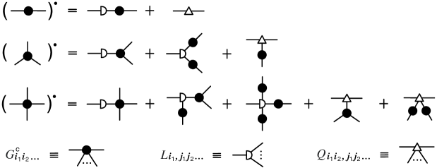
Figure 1: Diagrammatic representation of the evolution equations (16) for multipoint connected correlation functions. The dot on the left-hand side of each diagrammatic equation represents material derivative $u\cdot\partial$. The open half-circle with two legs represents $L_{i_{1},\,j_{1}}-\delta_{i_{1}j_{1}}(y_{1}\cdot\partial u)\cdot(\partial/\partial x_{1})$, i.e., it includes the first term on the right-hand side of each equation in (16). It is straightforward to generate the evolution equation for $G^{\rm c}_{n+1}$ recursively by adding in each diagram representing equation for $G^{\rm c}_{n}$ either one new leg to filled vertices or one new $G_{2}$ correlator to open vertices. This recursive rule can be readily verified using Eq. (23); see also Fig. 2. Similar diagrammatic representation applies to evolution equations (63) we derive below.

II.3 Arbitrary $n$

Our derivation can be extended beyond $n\leqslant 4$ to higher-order $n$-point functions, which are also of interest from the experimental point of view STAR:2022vlo . In this subsection we discuss generalization of Eqs. (15) and (16) to multipoint connected functions of arbitrary order $n$. In this work we do not need to use such general-$n$ equations, but these equations could facilitate the extension of our results to higher $n$ in future research. They also shed more light on the structure of the $n\leqslant 4$ equations we do use.

To start, we need to express correlators $G$ in terms of connected correlators $G^{\rm c}$, similarly to Eq. (15). The correlator $G_{i_{1}\dots i_{n}}$ is a sum of all possible nonequivalent products of $G^{\rm c}$ with indices ${i_{1}\dots i_{n}}$ divided between the $G^{\rm c}$ factors in all possible ways. As in Eq. (15) we can group these terms into sets within each of which the difference between the terms is a permutation of the indices; e.g., $G_{i_{1}i_{2}}G_{i_{3}i_{4}}+G_{i_{1}i_{3}}G_{i_{2}i_{4}}+G_{i_{1}i_{4}}G_{i_{2}i_{3}}$ is such a set. Using the permutation average notation Eq. (8) we can represent each such a set of terms by a single term. The resulting combinatorial factors will simply count the number of terms in each such “equivalent by permutation” set. We thus find the generalization of Eq. (15) in the form

$$G_{i_{1}\dots i_{n}}=\sum_{k=1}^{n}\sum_{\{n_{1},\dots,n_{k}\}}\{n_{1},\dots,n_{k}\}!\,G^{\rm c}_{\underbrace{i_{1}\dots i_{n_{1}}}_{n_{1}}}G^{\rm c}_{\underbrace{i_{n_{1}+1}\dots i_{n_{1}+n_{2}}}_{n_{2}}}\dots G^{\rm c}_{\underbrace{i_{n-n_{k}+1}\dots i_{n}}_{n_{k}}}\bigg{|}_{\overline{1\dots n}}\,,$$ (17)

where the inner sum is over all ordered sets of integer numbers $\{n_{1},\dots,n_{k}\}\in\mathbb{N}^{k}$, such that $n_{1}\leqslant n_{2}\leqslant\dots\leqslant n_{k}$ and $n_{1}+\dots+n_{k}=n$. Each set describes a partition of the $n$ indices $i_{1},\dots,i_{n}$ into $k$ groups

$$\underbrace{i_{1},\dots,i_{n_{1}}}_{n_{1}}|\underbrace{i_{n_{1}+1},\dots,i_{n_{1}+n_{2}}}_{n_{2}}|\dots|\underbrace{i_{n-n_{k}+1}\dots i_{n}}_{n_{k}}\,,$$ (18)

in a way that each term in the sum in Eq. (17) is different.

The factor $\{n_{1},\dots,n_{k}\}!\,$ is the order of the group of permutations of $n$ indices $i_{1},\dots,i_{n}$ which leaves the product of $G^{\rm c}$’s in Eq. (17) unchanged due to the symmetry of each $G^{\rm c}$ with respect to its own indices as well as the commutativity of the product of $G^{\rm c}$’s themselves. In other words, the factor counts how many identical terms of a given type appear in the sum over all $n!$ permutations of $n$ indices:

$$\{n_{1},\dots,n_{k}\}!\,\equiv\frac{n!}{n_{1}!\dots n_{k}!\,k_{1}!\dots k_{n}!}\,,$$ (19)

where $k_{m}$ is the count of times a given integer $m$ appears in the given set $\{n_{1},\dots,n_{k}\}$; e.g., for $n=7$ set $\{2,2,3\}$ the counts are $k_{1}=0$, $k_{2}=2$ and $k_{3}=1$. The denominator in Eq. (19) can be viewed as a symmetry factor corresponding to a diagram with $k$ vertices (factors of $G^{\rm c}$) with $n_{1},\dots,n_{k}$ equivalent legs (indices) each. In this picture, $k_{m}$ is the number of equivalent vertices with $m$ legs.

By definition, $k_{m}=0$ for $m>n$ and $\sum_{m}mk_{m}=n$. For a given $k$ in the outer sum in Eq. (17) all terms must obey $k_{1}+\dots+k_{n}=k$. This ensures that all terms in Eq. (17) with the same $k$ are of the same order in $\varepsilon$, i.e., $\mathcal{O}(\varepsilon^{n-k})$, according to Eq. (13).

The inverse of Eq. (17) gives connected correlator $G^{\rm c}$ in terms of correlators $G$’s:

$$G^{\rm c}_{i_{1}\dots i_{n}}=\sum_{k=1}^{n}\sum_{\{n_{1},\dots,n_{k}\}}(-1)^{k-1}(k-1)!\{n_{1},\dots,n_{k}\}!\,G_{\underbrace{i_{1}\dots i_{n_{1}}}_{n_{1}}}G_{\underbrace{i_{n_{1}+1}\dots i_{n_{1}+n_{2}}}_{n_{2}}}\dots G_{\underbrace{i_{n-n_{k}+1}\dots i_{n}}_{n_{k}}}\bigg{|}_{\overline{1\dots n}}\,.$$ (20)

This relation can be obtained by noting that the connected correlator generating function, $g_{\rm c}(\mu)=\sum_{n=1}^{\infty}\frac{1}{n!}G^{\rm c}_{n}\mu^{n}$, and the correlator generating function, $g(\mu)=1+\sum_{m=1}^{\infty}\frac{1}{m!}G_{m}\mu^{m}$, are related by $g_{\rm c}(\mu)=\ln g(\mu)$; i.e.,

$$\sum_{n=1}^{\infty}\frac{1}{n!}G^{\rm c}_{n}\mu^{n}=\ln\left(1+\sum_{m=1}^{\infty}\frac{1}{m!}G_{m}\mu^{m}\right)=\sum_{k=1}^{\infty}\frac{(-1)^{k-1}}{k}\left(\sum_{m=1}^{\infty}\frac{1}{m!}G_{m}\mu^{m}\right)^{k}\,,$$ (21)

where the logarithmic function is expanded in the last equality. Equating the terms of order $\mu^{n}$ on both sides, and noting that the contributions from $(\sum_{m}\frac{1}{m!}G_{m}\mu^{m})^{k}$ to the terms of order $\mu^{n}$ are simply given by

$$\sum_{\{n_{1},\dots,n_{k}\}}\frac{k!}{k_{1}!\dots k_{n}!}\frac{1}{n_{1}!\dots n_{k}!}G_{n_{1}}\dots G_{n_{k}}\mu^{n}$$ (22)

where $n_{1}+\dots+n_{k}=n$ and $k_{1}+\dots+k_{n}=k$, one obtains Eq. (20) immediately. For the sake of notation simplicity, we suppress the multivariable indices here, for instance, $G_{m}\mu^{m}\equiv G_{i_{1}\dots i_{m}}\mu_{i_{1}}\dots\mu_{i_{m}}$.

Using Eqs. (10), (13), (17), and (20), we arrive at the generic equation for $n$-point connected correlation function. At leading order ($\sim\varepsilon_{q}^{2}\varepsilon^{n-1}$) it can be obtained by induction from Eqs. (16) that

$$\,u\cdot\partial^{(x)}G^{\rm c}_{i_{1}\dots i_{n}}(x_{1},\dots,x_{n})=n\Big{[}-\left(y_{1}\cdot\partial u\right)\cdot\frac{\partial}{\partial x_{1}}G^{\rm c}_{i_{1}\dots i_{n}}(x_{1},\dots,x_{n})\\[2.0pt] +\sum_{k=1}^{n-1}\sum_{\begin{subarray}{c}\{n_{1},\dots,n_{k}\}\\ n_{1}+\dots+n_{k}=n-1\end{subarray}}\{n_{1},\dots,n_{k}\}!\,L_{i_{1},\,j_{1}\dots j_{k}}(x_{1})G^{\rm c}_{j_{1}\underbrace{i_{2}\dots}_{n_{1}}}(x_{1},x_{2},\dots)\dots G^{\rm c}_{j_{k}\underbrace{\dots i_{n}}_{n_{k}}}(x_{1},\dots,x_{n})\\[2.0pt] +(n-1)\sum_{k=0}^{n-2}\sum_{\begin{subarray}{c}\{n_{1},\dots,n_{k}\}\\ n_{1}+\dots+n_{k}=n-2\end{subarray}}\{n_{1},\dots,n_{k}\}!\,Q_{i_{1}i_{2},\,j_{1}\dots j_{k}}(x_{1},x_{2})G^{\rm c}_{j_{1}\underbrace{i_{3}\dots}_{n_{1}}}(x_{1},x_{3},\dots)\dots G^{\rm c}_{j_{k}\underbrace{\dots i_{n}}_{n_{k}}}(x_{1},\dots,x_{n})\Big{]}_{\overline{1\dots n}}\,.\\ \vspace{0mm}$$ (23)

The diagrammatic representation of Eq. (23) is sketched in Fig. 2.

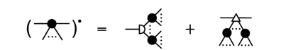
Figure 2: Diagrammatic representation of the evolution equations for generic multipoint connected correlation functions. Similarly to Fig. 1, the first term on the right-hand side of Eq. (23) is included into the diagram with an open semicircle with two legs. The last two terms are drawn in this figure, with all possible combinatorial arrangements at leading order. See Fig. 1 for the meaning of the diagram elements, and for the explicit representation of these diagrams when $n=2,3,4$.

II.4 Confluent formalism for multipoint equal-time correlators

An important ingredient for our derivation of the fluctuation evolution equations in relativistic hydrodynamics is the confluent formalism, which allows us to covariantly describe fluctuations in the local rest frame of the fluid. We follow the approach introduced in Ref. An:2019rhf for two-point correlators, but generalize it here to arbitrary $n$-point correlators. Most of the notations in this section are similar to the ones introduced in Ref. An:2019rhf and are summarized in Appendix D for convenience.

The four-velocities $u$ of the flow in two space-time points $x$ and $x+\Delta x$ can be related by a Lorentz boost $\Lambda$ which we define as

$$\Lambda(\Delta x)u(x+\Delta x)=u(x)\,.$$ (24)

For infinitesimal $\Delta x$, the four-velocities are different by infinitesimal amount $\Delta u=(\Delta x\cdot\partial)u$ and the boost can be represented by the following matrix close to unity

$$\Lambda(\Delta x)={\mathbb{1}}+\Delta\Lambda\,,\quad\mbox{where}\quad\Delta\Lambda_{\mu}^{~{}\nu}(\Delta x)=-u_{\mu}\Delta u^{\nu}+u^{\nu}\Delta u_{\mu}\,.$$ (25)

For $n$-point function the fluctuations of the $n$ variables are evaluated at different points $(x_{1},\ldots,x_{n})$ with different local velocities $u(x_{i})$. Before comparing or correlating these local variables it is natural to boost all of them to the same local rest frame at the midpoint

$$x\equiv\sum_{i=1}^{n}\frac{x_{i}}{n}.$$ (26)

If the variables are components of a four-vector (such as $\delta u^{\mu}$), then the boost mixes those components using matrix $\Lambda$ given explicitly in Eq. (25). If the variables are scalars (such as $\delta m$ or $\delta p$) the boost is trivial (identity), or $\Delta\Lambda=0$. To treat these two cases simultaneously in our formalism, we introduce (as in Ref. An:2019rhf ) an object $u^{i}$ whose components equal to $u^{\mu}$ when $i=0,\dots,3$, and zero for all other values of $i$, corresponding to scalar hydrodynamic variables. Then we can express infinitesimal boost from $x+\Delta x$ to $x$, as a matrix

$$\Delta\Lambda_{i}^{~{}j}(\Delta x)=-\Delta x^{\mu}\bar{\omega}_{\mu i}^{j}\,,$$ (27)

where we defined the confluent connection as in Ref. An:2019rhf ,

$$\bar{\omega}_{\mu i}^{j}=u_{i}\partial_{\mu}u^{j}-u^{j}\partial_{\mu}u_{i}\,.$$ (28)

Boosting all variables into the local rest frame at the midpoint using $\Lambda(x_{i}-x)$, we can then define the confluent $n$-point correlator $\bar{G}$ and express it in terms of the “raw” correlators $G$:

$$\bar{G}_{i_{1}\dots i_{n}}(x_{1},\dots,x_{n})\equiv\Lambda_{i_{1}}^{~{}j_{1}}(x_{1}-x)\ldots\Lambda_{i_{n}}^{~{}j_{n}}(x_{n}-x)G_{j_{1}\dots j_{n}}(x_{1},\dots,x_{n})$$

$$\approx\,\, G_{i_{1}\dots i_{n}}(x_{1},\dots,x_{n})-n\left[(x_{1}-x)^{\mu}\bar{\omega}^{j_{1}}_{\mu i_{1}}G_{j_{1}i_{2}\dots i_{n}}(x_{1},\dots,x_{n})\right]_{\overline{1\dots n}}\,,$$ (29)

where in the second line we have kept only the leading term in the expansion in powers of $x_{i}-x$. The idea of the confluent correlator is illustrated in Fig. 3.

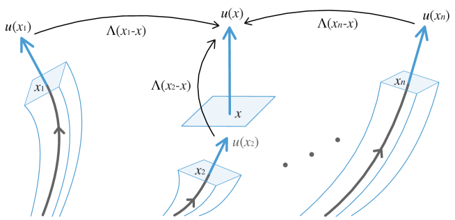
Figure 3: An illustration, in space-time, of the process involved in constructing the confluent $n$-point function $\bar{G}$ from the “raw” $n$-point function $G$. All $n$ fluctuation fields are boosted from their respective local rest frames at $x_{i}$ to the same frame at the midpoint $x$.

In order to describe the rate of change of a correlation function such as $\bar{G}_{n}$ with respect to the midpoint position $x$, we want to compare the values of $\bar{G}_{n}$ at two sets of arguments $x_{i}$ and $x_{i}^{\prime}$. The ordinary derivative would correspond to $x_{i}^{\prime}=x_{i}+\Delta x$ with the same $\Delta x$ for all $i$. A more natural measure in the context of hydrodynamics, however, would take into account the change of the four-velocity between the old midpoint $x$ and the new midpoint $x^{\prime}=x+\Delta x$. Specifically, we want to evaluate the function at a new set of arguments (points $x_{i}^{\prime}$), which are located relative to the new midpoint $x^{\prime}$ in exactly the same way (in the sense to be precisely defined below) as they were around $x$ in the rest frame at midpoint. This is essential if we want to evaluate the rate of change of an equal-time correlator.

That rest frame defined by the four-velocity $u(x+\Delta x)$, in general, is different from $u(x)$. The relative position of the points can be described by four-vectors

$$y_{i}(x)\equiv x_{i}-x\,.$$ (30)

In order to preserve the relative positions in the rest frame at the midpoint we shall define new relative positions using the same boost as in Eq. (24), i.e., $y_{i}(x+\Delta x)=\Lambda(\Delta x)^{-1}y_{i}(x)$. This would ensure, in particular, that the time components of the relative four-vectors $y_{i}(x)$ in the rest frame are preserved: $y_{i}(x)\cdot u(x)=y_{i}(x+\Delta x)\cdot u(x+\Delta x)$. Which means that if we define equal-time correlator by $y_{i}(x)\cdot u(x)=0$, the same relation remain true at the new point: $y_{i}(x+\Delta x)\cdot u(x+\Delta x)=0$. In other words, if the points $x_{i}$ are equal-time in the frame at their midpoint, so are the points $x^{\prime}_{i}$.

Therefore, we define the confluent derivative via the following relation, where $\Delta x$ is infinitesimal:

$$\Delta x\cdot\bar{\nabla}\bar{G}_{i_{1}\dots i_{n}}\equiv\,\Lambda(\Delta x)_{i_{1}}^{~{}j_{1}}\ldots\Lambda(\Delta x)_{i_{n}}^{~{}j_{n}}\bar{G}_{j_{1}\dots j_{n}}(x_{1}^{\prime},\dots,x_{n}^{\prime})-\bar{G}_{i_{1}\dots i_{n}}(x_{1},\dots,x_{n})\,,\\[2.0pt] \quad\mbox{where}\quad x_{i}^{\prime}=x+\Delta x+\Lambda(\Delta x)^{-1}y_{i}(x)\quad\mbox{and}\quad x_{i}=x+y_{i}(x)\,.$$ (31)

Note that the variables which are being correlated are also boosted accordingly to make sure that only their change with respect to the local rest frame is measured, and not the change of the components of these variables due to the change of the rest frame itself. Taking the limit $\Delta x\to 0$ we can write Eq. (31) in terms of the partial derivatives of $G$ and the boost connection $\bar{\omega}$:

$$\bar{\nabla}_{\mu}\bar{G}_{i_{1}\dots i_{n}} \equiv n\left[\left(\frac{\partial}{\partial x_{1}^{\mu}}-\bar{\omega}_{\mu\beta}^{\alpha}y_{1}^{\beta}\frac{\partial}{\partial x_{1}^{\alpha}}\right)\bar{G}_{i_{1}\dots i_{n}}-\bar{\omega}_{\mu i_{1}}^{j_{1}}\bar{G}_{j_{1}\dots i_{n}}\right]_{\overline{1\dots n}}\,.$$ (32)

At this point it is convenient to introduce the derivative with respect to the midpoint, $x$ which was already defined in Eq. (10), as well as the derivatives with respect to separation vectors $y_{i}$ at fixed midpoint $x$:

$${\partial^{(x)}}\equiv\sum_{i=1}^{n}\frac{\partial}{\partial x_{i}}\,,\quad\partial^{(y_{i})}\equiv\frac{\partial}{\partial x_{i}}-\frac{1}{n}\sum_{j=1}^{n}\frac{\partial}{\partial x_{j}}\equiv\frac{\partial}{\partial x_{i}}-\frac{1}{n}\frac{\partial}{\partial x}\,.$$ (33)

Note that $y_{i}$ variables are not independent, since $\sum_{i=1}^{n}y_{i}=0$, so the derivative $\partial^{(y_{i})}$ has unusual, but simple, properties, e.g., $\partial^{(y_{i})}x=0$, $\partial^{(y_{i})}y_{j}=\delta_{ij}-1/n$. In terms of such derivatives Eq. (32) reads

$$\bar{\nabla}_{\mu}\bar{G}_{i_{1}\dots i_{n}} \equiv\partial^{(x)}_{\mu}\bar{G}_{i_{1}\dots i_{n}}-n\left[\bar{\omega}_{\mu\beta}^{\alpha}y_{1}^{\beta}\partial^{(y_{1})}_{\alpha}\bar{G}_{i_{1}\dots i_{n}}+\bar{\omega}_{\mu i_{1}}^{j_{1}}\bar{G}_{j_{1}\dots i_{n}}\right]_{\overline{1\dots n}}\,.$$ (34)

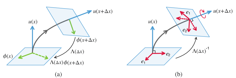
Figure 4: The origin of two connections $\bar{\omega}$ and $\mathring{\omega}$ in the confluent derivative applying to confluent $n$-point functions. Panel (a) explains the origin of boost connection $\bar{\omega}$, brought out by boosting the fluctuation variable $\phi(x+\Delta x)$ from the local rest frame of $u(x+\Delta x)$ to the local rest frame of $u(x)$, i.e., $\Lambda(\Delta x)\phi(x+\Delta x)$, using the same boost that takes velocity $u(x+\Delta x)$ to $u(x)$. The action of the boost on $\phi$ is determined by the tensor rank of $\phi$ and is illustrated in the figure for the case of a four-vector (e.g., velocity fluctuation). Panel (b) explains the origin of spin connection due to the confluent motion of equal-time surface and the arbitrariness of the local triad $e_{a}$ choice. Under the boost from the local rest frame of $u(x)$ to $u(x+\Delta x)$ every coordinate vector $y$ in the local equal-time three-hyperplane (represented by the blue rectangle), subject to the constraint $u(x)\cdot y=0$, must also be boosted simultaneously by $\Lambda(\Delta x)^{-1}$. This includes the basis $e_{a}(x)$ in that hyperplane (red vectors, only two dimensions $a=1,2$ are shown). Upon the boost the basis vectors map onto $\Lambda(\Delta x)^{-1}e_{a}(x)$ (dashed red vectors) at point $x+\Delta x$ . The additional rotation (indicated by the red circular arrow) in the equal-time plane needed to align the boosted basis (dashed red) with the local basis $e_{a}(x+\Delta x)$ (solid red) gives rise to the $\mathring{\omega}$ connection.

Another derivative which will be even more useful when discussing the Wigner transform is obtained by introducing the local tetrad consisting of vector $u(x)$ and a triad $e_{a}(x)$, $a=1,2,3$, thus expressing vector $y$ in components: $y(x)=e_{a}(x)y^{a}+u(x)y^{u}$, where $y^{u}=-u(x)\cdot y$ is the time component in the local rest frame at point $x$. In this paper we shall only consider equal-time correlators, so we work with $y^{u}=0$ (cf. Fig. 5(a)). We can then define a derivative where $y^{a}$ and $y^{u}=0$ are fixed, i.e.,

$$\Delta x\cdot\mathring{\partial}\bar{G}_{i_{1}\dots i_{n}}\equiv\,\bar{G}_{i_{1}\dots i_{n}}(x_{1}^{\prime},\dots,x_{n}^{\prime})-\bar{G}_{i_{1}\dots i_{n}}(x_{1},\dots,x_{n})\,,\\[2.0pt] \quad\mbox{where}\quad x_{i}^{\prime}=x+\Delta x+e_{a}(x+\Delta x)y^{a}_{i}\quad\mbox{and}\quad x_{i}=x+e_{a}(x)y^{a}_{i}\,.$$ (35)

Taking the limit $\Delta x\to 0$ we find:

$$\mathring{\partial}_{\mu}\bar{G}_{i_{1}\dots i_{n}}\equiv n\left[\left(\frac{\partial}{\partial x_{1}^{\mu}}+\mathring{\omega}_{\mu b}^{a}y_{1}^{b}\frac{\partial}{\partial x_{1}^{a}}+(\partial_{\mu}u_{\lambda})y_{1}^{\lambda}\left(u\cdot\frac{\partial}{\partial x_{1}}\right)\right)\bar{G}_{i_{1}\dots i_{n}}\right]_{\overline{1\dots n}}\\[2.0pt] =\partial^{(x)}_{\mu}\bar{G}_{i_{1}\dots i_{n}}+n\left[\mathring{\omega}_{\mu b}^{a}y_{1}^{b}\partial^{(y_{1})}_{a}\bar{G}_{i_{1}\dots i_{n}}-\bar{\omega}_{\mu\lambda}^{\nu}y_{1}^{\lambda}\partial^{(y_{1})}_{\nu}\bar{G}_{i_{1}\dots i_{n}}\right]_{\overline{1\dots n}}$$ (36)

where we introduced

$$\mathring{\omega}_{\mu b}^{a}\equiv e_{\nu}^{a}\partial_{\mu}e^{\nu}_{b}$$ (37)

with $a,b=1,2,3$; the connection associated with the freedom of choice of the local basis triad $e_{a}$ at each point $x$. Using this connection we expressed the derivatives of $e_{a}$ appearing in Eq. (36) as

$$\partial_{\mu}e^{\nu}_{a}=(e^{\nu}_{b}e^{b}_{\lambda}-u^{\nu}u_{\lambda})\partial_{\mu}e^{\lambda}_{a}=e^{\nu}_{b}\mathring{\omega}^{b}_{\mu a}+{e^{\lambda}_{a}u^{\nu}(\partial_{\mu}u_{\lambda})}=e^{\nu}_{b}\mathring{\omega}^{b}_{\mu a}-{e^{\lambda}_{a}\bar{\omega}^{\nu}_{\mu\lambda}}$$ (38)

where we also used Eq. (28) and $u\cdot y_{i}=0$. We also defined the derivative

$$\partial^{(y)}_{a}\equiv e_{a}^{\mu}\partial^{(y)}_{\mu}\,,$$ (39)

which is essentially the derivative with respect to three-component vector $y^{a}$, which, similarly to $\partial^{(y_{i})}_{\mu}$ defined in Eq. (33), is preserving the constraint $\sum_{i=1}^{n}y_{i}=0$.

Substituting Eq. (36) into Eq. (34), we find the relationship between the derivatives we defined:

$$\bar{\nabla}_{\mu}\bar{G}_{i_{1}\dots i_{n}} \equiv\mathring{\partial}_{\mu}\bar{G}_{i_{1}\dots i_{n}}-n\left[\mathring{\omega}_{\mu b}^{a}y_{1}^{b}\partial^{(y_{1})}_{a}\bar{G}_{i_{1}\dots i_{n}}+\bar{\omega}_{\mu i_{1}}^{j_{1}}\bar{G}_{j_{1}\dots i_{n}}\right]_{\overline{1\dots n}}\,.$$ (40)

The confluent derivative in Eq. (40) incorporating the two connections defined in Eqs. (28) and (37) is illustrated in Fig. 4.

Considering now a connected correlation function, $G^{\text{c}}(x_{1},\ldots,x_{n})$ (see Eq. (15)), and using the generalized Wigner transform introduced in Ref. An_2021 we define the Wigner function

$$W_{n}(x;\bm{q}_{1},\dots,\bm{q}_{n})=\mathop{\text{\Large$\int$}}\nolimits\left[\prod_{i=1}^{n}d^{3}y_{i}^{a}\,e^{-iq_{ia}y_{i}^{a}}\right]\delta^{(3)}\left(\frac{1}{n}\sum_{i=1}^{n}y_{i}^{a}\right)\bar{G}_{n}^{\text{c}}(x+e_{a}y_{1}^{a},\ldots,x+e_{a}y_{n}^{a})\,.$$ (41)

where $q^{a}$ denote components of three-vector ${\bm{q}}=\{q^{a}\}\in{\mathbb{R}}^{3}$ with $a=1,2,3$ which is the wave number conjugate to vector $y^{a}$. To avoid clutter in our notation, we replaced the indices $i_{1},\ldots,i_{n}$, which are the same on $W_{i_{1}\ldots i_{n}}$ and $\bar{G}^{\text{c}}_{i_{1}\ldots i_{n}}$, with a single index $n$. The inverse transformation of Eq. (41) is given by

$$\bar{G}_{n}^{\text{c}}(x+e_{a}y_{1}^{a},\ldots,x+e_{a}y_{n}^{a})=\mathop{\text{\Large$\int$}}\nolimits\left[\prod_{i=1}^{n}\frac{d^{3}\bm{q}_{i}}{(2\pi)^{3}}\,e^{iq_{ia}y_{i}^{a}}\right]\delta^{(3)}\left(\sum_{i=1}^{n}\frac{\bm{q}_{i}}{2\pi}\right)W_{n}(x;\bm{q}_{1},\dots,\bm{q}_{n})\,.$$ (42)

Some of the features of this transformation of variables are illustrated in Fig. 5. In particular we note that, due to the constraint $\sum_{i}y_{i}=0$ implemented by the delta function in Eq. (41), the Wigner function is invariant with respect to the shift of all wave numbers $\bm{q}_{i}$ by the same vector. That means we can constrain the value of $\sum_{i}\bm{q}_{i}$ without losing any information about the dependence of $W$ on its arguments (of course, this is related to the fact that $W_{n}$ has one argument more than $G_{n}$). The natural choice of the constraint is $\sum_{i}\bm{q}_{i}=0$ as in Eq. (42). An intuitive way to understand this is to think of $W_{n}$ as an $n$-point “amplitude” and of $\bm{q}_{i}$ as the corresponding “momenta” flowing in. Then the constraint is simply a reflection of “momentum” conservation.

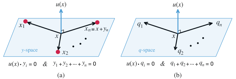
Figure 5: An illustration of the vectors relevant to the Wigner transform of equal-time confluent correlators living in coordinate $y$-space (shown in panel (a)) to Wigner functions living in wave number $\bm{q}$-space (shown in panel (b)). The wave numbers drawn in the figure are four-vectors $e^{\mu}_{a}q^{a}\equiv q^{\mu}$. The nature of the constraint $\sum_{i}\bm{q}_{i}=0$ is discussed in the text.

It is easy to see that the derivative of the Wigner function with respect to $x$ at fixed $\bm{q}_{i}$’s,

$$\Delta x\cdot\mathring{\partial}W_{n}(x;\bm{q}_{1},\ldots,\bm{q}_{n})=W_{n}(x+\Delta x;\bm{q}_{1},\ldots,\bm{q}_{n})-W_{n}(x;\bm{q}_{1},\ldots,\bm{q}_{n})\,,$$ (43)

is the Wigner transform of $\mathring{\partial}\bar{G}^{\text{c}}$; i.e., the derivative $\mathring{\partial}$ commutes with the Wigner transform.

It is also easy to see that the derivative defined in Eqs. (39) and (33) upon Wigner transform becomes simply the multiplication by the corresponding $iq_{a}$:

$$\partial_{a}^{(y_{i})}\quad\ext@arrow 0099\arrowfill@\relbar\relbar\longrightarrow{}{~{}~{}\text{W.T.}~{}~{}}\quad iq_{ia}\,.$$ (44)

We shall define $\bar{\nabla}W$ as Wigner transform of $\bar{\nabla}\bar{G}^{\text{c}}$. Using Eq. (34) it is then easy to show that

$$\bar{\nabla}_{\mu}W_{i_{1}\dots i_{n}}=\mathring{\partial}_{\mu}W_{i_{1}\dots i_{n}}+n\left(\mathring{\omega}_{\mu b}^{a}q_{1a}\frac{\partial}{\partial q_{1b}}W_{i_{1}\dots i_{n}}-\bar{\omega}_{\mu i_{1}}^{j_{1}}W_{j_{1}i_{2}\dots i_{n}}\right)_{\overline{1\dots n}}\,.$$ (45)

Now let us turn to the derivation of the evolution equation of connected Wigner functions. Applying the confluent derivative in Eq. (45) along $u(x)$ to Eq. (41), we express the result in terms of the “raw” connected correlation functions $G^{\text{c}}$ as follows:

$$u\cdot\bar{\nabla}W_{i_{1}\dots i_{n}}(x;\bm{q}_{1},\dots,\bm{q}_{n})=u\cdot\mathring{\partial}W_{i_{1}\dots i_{n}}-nu^{\mu}\left(\bar{\omega}_{\mu i_{1}}^{j_{1}}W_{j_{1}i_{2}\dots i_{n}}-\mathring{\omega}_{\mu b}^{a}q_{1a}\frac{\partial}{\partial q_{1b}}W_{i_{1}\dots i_{n}}\right)_{\overline{1\dots n}}$$

$$= \mathop{\text{\Large$\int$}}\nolimits\left[\prod_{i=1}^{n}d^{3}y_{i}\,e^{-iq_{ia}y_{i}^{a}}\right]\,\delta^{(3)}\left(\frac{1}{n}\sum_{i=1}^{n}y_{i}\right)\Big{\{}u\cdot\partial G^{\rm c}_{i_{1}\dots i_{n}}$$

$$\qquad-n\left[\left(u^{\mu}\bar{\omega}^{\nu}_{\mu\lambda}y_{1}^{\lambda}\partial_{\nu}^{(y_{1})}\delta_{i_{1}}^{j_{1}}+y_{1}^{\mu}\bar{\omega}^{j_{1}}_{\mu i_{1}}u\cdot\partial+u^{\mu}\bar{\omega}_{\mu i_{1}}^{j_{1}}\right)G^{\rm c}_{j_{1}i_{2}\dots i_{n}}\right]_{\overline{1\dots n}}\Big{\}}\,,$$ (46)

where we used Eqs. (II.4), (34) and (36).

We then apply the evolution equations (16) (and, generically, Eq. (23)) for $G_{n}^{\rm c}$ to convert local rest frame time derivatives $u\cdot\partial$ into spatial derivatives and perform the inverse Wigner transform using Eq. (42). As a result, we express the confluent local rest frame time derivative of the Wigner function on the left-hand side of Eq. (II.4) in terms of the Wigner functions themselves, thus obtaining a set of local evolution equations.

The explicit form of the evolution equations for Wigner functions will depend on the explicit form of multilinear operators $L$ and $Q$ in Eqs. (16) that need to be substituted into Eq. (II.4). Below we shall obtain this explicit form for an important subset of correlators in hydrodynamics.

III Specific entropy fluctuations in relativistic hydrodynamics

III.1 Stochastic equation for specific entropy fluctuations

With the generic formalism established, we now apply it to a more specific hydrodynamic framework governed by the local equations for the conservation of energy, momentum, and charge:

$$\partial_{\mu}\breve{T}^{\mu\nu}=0\,,$$ (47a)

$$\partial_{\mu}\breve{J}^{\mu}=0\,,$$ (47b)

supplemented by constitutive relations for the stress tensor $T^{\mu\nu}$ and charge current $J^{\mu}$ in the Landau frame for the stochastic relativistic hydrodynamics Kapusta:2011gt ,

$$\breve{T}^{\mu\nu} =\breve{\epsilon}\breve{u}^{\mu}\breve{u}^{\nu}+\breve{p}\breve{\Delta}^{\mu\nu}+\breve{\Pi}^{\mu\nu}+\breve{S}^{\mu\nu}\,,$$ (48a)

$$\breve{J}^{\mu} =\breve{n}\breve{u}^{\mu}+\breve{\nu}^{\mu}+\breve{I}^{\mu}\,,$$ (48b)

where $\epsilon$ and $n$ are the energy density and charge density respectively, measured in the local rest frame; $u$ is the four-velocity already introduced in Eq. (1); $\Delta_{\mu\nu}=g_{\mu\nu}+u_{\mu}u_{\nu}$ is the transverse projection operator satisfying $\Delta^{\mu\nu}u_{\nu}=0$; the pressure $p$, appearing as the coefficient of $\Delta^{\mu\nu}$ in the ideal part of the stress tensor, is determined by chosen primary hydrodynamic variables (such as $\epsilon$ and $n$) through the equation of state. The explicit forms of the dissipative parts, denoted by $\Pi^{\mu\nu}$ and $\nu^{\mu}$ for stress tensor and charge current respectively, are determined by applying the second law of thermodynamics Landau:2013fluid :

$$\Pi^{\mu\nu}\equiv-2\eta\sigma^{\mu\nu}-\zeta\theta\Delta^{\mu\nu}\,,\qquad\nu^{\mu}\equiv-\lambda\Delta^{\mu}_{~{}\nu}\partial^{\nu}\alpha\,,$$ (49)

where $\alpha\equiv\beta\mu\equiv{\mu}/{T}$ is the chemical potential to temperature ratio, and gradients of velocity are decomposed into the traceless and trace parts where

$$\sigma^{\mu\nu}\equiv\theta^{\mu\nu}-\frac{1}{3}\theta\Delta^{\mu\nu}\,,\quad\theta^{\mu\nu}\equiv\frac{1}{2}\Delta^{\mu\alpha}\Delta^{\nu\beta}(\partial_{\alpha}u_{\beta}+\partial_{\beta}u_{\alpha})\,,\quad\theta\equiv\theta^{\mu}_{\mu}=\partial\cdot u\,.$$ (50)

The transport coefficients, denoted by $\eta$, $\zeta$ and $\lambda$ above, are shear viscosity, bulk viscosity and charge conductivity respectively.

Eqs. (48), accompanied by the constitutive equations (48) become stochastic due to the presence of the microscopic scale noises $\breve{I}^{\mu}$ and $\breve{S}^{\mu\nu}$. The noises are defined similarly to Eqs. (1) and (2):

$$\breve{I}^{\mu}=\breve{H^{I}}^{\mu}_{a}\eta^{I}_{a}\,,\quad\mbox{where}\quad\langle\eta^{I}_{a}(x_{1})\eta^{I}_{b}(x_{2})\rangle=2\delta_{ab}\delta^{(4)}(x_{1}-x_{2})\quad\mbox{and}\quad{H^{I}}^{\mu}_{a}=\sqrt{\lambda}e^{\mu}_{a}\,,$$ (51)

with $a=1,2,3$ since there are three independent noises (random currents) in the local rest frame, and $e^{\mu}_{a}$ is an arbitrary spatial basis triad in the local rest frame: $e_{a}\cdot u=0$ (as already defined and discussed in Ref. An:2019rhf and in the previous section). As a result $({H^{I}}^{\mu}_{a}){H^{I}}^{\nu}_{a}=\lambda\Delta^{\mu\nu}$ (note that the choice of the triad $e_{a}$ does not matter, since $e^{\mu}_{a}e^{\nu}_{a}=\Delta^{\mu\nu}$). We define $\breve{S}^{\mu\nu}$ accordingly. Since there are six independent noise variables (corresponding to random stress tensor in local rest frame), the components of $\breve{S}^{\mu\nu}$ are expressed in terms of a symmetric rank-three random matrix $\eta^{S}_{ab}$, i.e.,

$$\breve{S}^{\mu\nu}=\breve{H^{S}}^{\mu\nu}_{ab}\eta^{S}_{ab}\,,\quad\mbox{where}\quad\langle\eta^{S}_{ab}(x_{1})\eta^{S}_{cd}(x_{2})\rangle=(\delta_{ac}\delta_{bd}+\delta_{ad}\delta_{bc})\delta^{(4)}(x_{1}-x_{2})\\[4.0pt] \quad\mbox{and}\quad{H^{S}}^{\mu\nu}_{ab}=\sqrt{\frac{T\eta}{2}}\left(e^{\mu}_{a}e^{\nu}_{b}+e^{\mu}_{b}e^{\nu}_{a}-\frac{2}{3}\Delta^{\mu\nu}\delta_{ab}\right)+\sqrt{\frac{T\zeta}{3}}\Delta^{\mu\nu}\delta_{ab}\,.$$ (52)

Similarly to Eqs. (51) and (52), isotropy requires that the random current and stress noises are statistically independent:

$$\begin{gathered}\langle{\eta^{I}_{a}(x_{1})\eta^{S}_{bc}(x_{2})}\rangle=0\,.\end{gathered}$$ (53)

We now turn our focus to the fluctuations of specific entropy (i.e., ratio of entropy density $s$ to charge density $n$), $m\equiv s/n$, which is parametrically the slowest and also the most significant hydrodynamic mode near a liquid-gas critical point, as we already discussed in Section I, such a focus also underlies the Hydro+ approach in Ref. Stephanov:2018hydro+ .

Specifically, we are going to derive deterministic equations of motion for the correlators of $m$. To achieve this, we first obtain the stochastic equation for the evolution of $\breve{m}$ starting from the conservation equation (47). We find

$$\breve{u}\cdot\partial\breve{m} =\breve{m}_{n}\partial^{\mu}\breve{\lambda}\breve{\Delta}_{\mu\nu}\partial^{\nu}\breve{\alpha}+2\breve{m}_{\epsilon}\breve{\eta}\breve{\sigma}^{\mu\nu}\breve{\sigma}_{\mu\nu}+\breve{m}_{\epsilon}\breve{\zeta}\breve{\theta}^{2}+\xi_{m}\,,$$ (54)

where

$$m_{n}\equiv\left(\frac{\partial m}{\partial n}\right)_{\!\epsilon}=-\frac{\beta w}{n^{2}}\,,\qquad m_{\epsilon}\equiv\left(\frac{\partial m}{\partial\epsilon}\right)_{\!n}=\frac{\beta}{n}$$ (55)

are expressed in terms of independent thermodynamic derivatives chosen in the set I given by Table 1 in Appendix. A, and

$$\xi_{m}=-\breve{m}_{n}\partial_{\mu}\breve{I}^{\mu}+\breve{m}_{\epsilon}\breve{u}_{\nu}\partial_{\mu}\breve{S}^{\mu\nu}\,.$$ (56)

Eq. (54) has a form similar to Eq. (1) with $\psi=m$. Therefore the formalism of the previous section can be applied. To obtain the equation corresponding to Eq. (6), we expand Eq. (54) in the fluctuation field, $\delta m$, as well as in derivatives applying to fluctuation fields, such as $\partial\delta m=\mathcal{O}(q)$, up to $\mathcal{O}(q^{2})$. It is sufficient to truncate the expansion at order $\delta m^{3}$ to obtain equations for the four-point connected functions.

While we are interested in correlators of $\delta m$, the evolution of $\delta m$ also depends on fluctuations of other hydrodynamic variables, in particular, on fluctuations of pressure, $\delta p$. As a result, the evolution of the correlators of $\delta m$ will depend on correlators of $\delta p$ as well. As we shall see below, to the leading order in hydrodynamic (gradient) expansion and in the regime we consider, we only need to include terms linear in $\delta p$. Correspondingly, if we only write the terms which will contribute to the correlator evolution equations in the regime we consider (e.g., Eqs. (61) or (63)), we find

$$u\cdot\partial\delta m=:u\cdot\partial\breve{m}:\,\equiv~{}u\cdot\partial\breve{m}-\langle{u\cdot\partial\breve{m}}\rangle=\,\,:L_{m,m}\delta m+L_{m,p}\delta p+\frac{1}{2}L_{m,mm}\delta m\delta m+L_{m,mp}\delta m\delta p\\ +\frac{1}{6}L_{m,mmm}\delta m\delta m\delta m+\frac{1}{2}L_{m,mmp}\delta m\delta m\delta p+\xi_{m}:$$ (57)

The multilinear operators $L_{m,m\dots m}$ serving as expansion coefficients are more explicitly written as

$$L_{m,m}\delta m\equiv L_{m,m}[\delta m]=m_{n}\partial^{\mu}\lambda\Delta_{\mu\nu}\partial^{\nu}\alpha_{m}\delta m+m_{n}\partial^{\mu}\lambda_{m}\delta m\Delta_{\mu\nu}\partial^{\nu}\alpha+(m_{n})_{,m}\delta m\partial^{\mu}\lambda\Delta_{\mu\nu}\partial^{\nu}\alpha\\[2.0pt] =m_{n}\lambda\alpha_{m}\Delta_{\mu\nu}\partial^{\mu}\partial^{\nu}\delta m+\mathcal{O}(kq)\,,$$ (58a)

$$L_{m,p}\delta p\equiv L_{m,p}[\delta p]=m_{n}\partial^{\mu}\lambda\Delta_{\mu\nu}\partial^{\nu}\alpha_{p}\delta p+m_{n}\partial^{\mu}\lambda_{p}\delta p\Delta_{\mu\nu}\partial^{\nu}\alpha+(m_{n})_{,p}\delta p\partial^{\mu}\lambda\Delta_{\mu\nu}\partial^{\nu}\alpha\\[2.0pt] =m_{n}\lambda\alpha_{p}\Delta_{\mu\nu}\partial^{\mu}\partial^{\nu}\delta p+\mathcal{O}(kq)\,,$$ (58b)

$$L_{m,mm}\delta m\delta m\equiv L_{m,mm}[\delta m,\delta m]\\[2.0pt] =m_{n}\lambda\alpha_{mm}\Delta_{\mu\nu}\partial^{\mu}\partial^{\nu}\delta m^{2}+2m_{n}\lambda_{m}\alpha_{m}\Delta_{\mu\nu}\partial^{\mu}\delta m\partial^{\nu}\delta m+2(m_{n})_{,m}\lambda\alpha_{m}\Delta_{\mu\nu}\delta m\partial^{\mu}\partial^{\nu}\delta m+\mathcal{O}(kq)\,,$$ (58c)

$$L_{m,mp}\delta m\delta p\equiv L_{m,mp}[\delta m,\delta p]\\[2.0pt] =m_{n}\lambda\alpha_{mp}\Delta_{\mu\nu}\partial^{\mu}\partial^{\nu}\delta m\delta p+m_{n}\lambda_{m}\alpha_{p}\Delta_{\mu\nu}\partial^{\mu}\delta m\partial^{\nu}\delta p+m_{n}\lambda_{p}\alpha_{m}\Delta_{\mu\nu}\partial^{\mu}\delta p\partial^{\nu}\delta m\\[2.0pt] +(m_{n})_{,m}\lambda\alpha_{p}\Delta_{\mu\nu}\delta m\partial^{\mu}\partial^{\nu}\delta p+(m_{n})_{,p}\lambda\alpha_{m}\Delta_{\mu\nu}\delta p\partial^{\mu}\partial^{\nu}\delta m+\mathcal{O}(kq)\,,$$ (58d)

$$L_{m,mmm}\delta m\delta m\delta m\equiv L_{m,mmm}[\delta m,\delta m,\delta m]\\[2.0pt] =m_{n}\partial^{\mu}\lambda\alpha_{mmm}\Delta_{\mu\nu}\partial^{\nu}\delta m^{3}+3m_{n}\lambda_{m}\alpha_{mm}\Delta_{\mu\nu}\partial^{\mu}\delta m\partial^{\nu}\delta m^{2}+3(m_{n})_{,m}\lambda\alpha_{mm}\Delta_{\mu\nu}\delta m\partial^{\mu}\partial^{\nu}\delta m^{2}\\[2.0pt] +3m_{n}\lambda_{mm}\alpha_{m}\Delta_{\mu\nu}\partial^{\mu}\delta m^{2}\partial^{\nu}\delta m+6(m_{n})_{,m}\lambda_{m}\alpha_{m}\Delta_{\mu\nu}\delta m\partial^{\mu}\delta m\partial^{\nu}\delta m\\[2.0pt] +3(m_{n})_{,mm}\lambda\alpha_{m}\Delta_{\mu\nu}\delta m^{2}\partial^{\mu}\partial^{\nu}\delta m+\mathcal{O}(kq)\,,$$ (58e)

where

$$\alpha_{\underbrace{{}_{m\dots m}}_{k}\underbrace{{}_{p\dots p}}_{\ell}}\equiv\left(\frac{\partial^{\ell}}{\partial p^{\ell}}\left(\frac{\partial^{(k)}\alpha}{\partial m^{k}}\right)_{p}\right)_{m}\,,\qquad\lambda_{\underbrace{{}_{m\dots m}}_{k}\underbrace{{}_{p\dots p}}_{\ell}}\equiv\left(\frac{\partial^{(\ell)}}{\partial p^{\ell}}\left(\frac{\partial^{(k)}\lambda}{\partial m^{k}}\right)_{p}\right)_{m}\,.$$ (59)

In Eqs. (58) derivative $\partial$ applies to all factors to the right of it, and, since we only consider fluctuations of $m$, i.e., $i,j_{1},\dots,j_{n}=m$ and $u_{,m\dots m}=0$ in Eq. (7), we have $L_{m,m\dots m}=F_{m,m\dots m}$.

The noise introduced in Eq. (56) satisfies

$$Q_{mm}(x_{1},x_{2}) =\frac{1}{2}\langle{\xi_{m}(x_{1})\xi_{m}(x_{2})}\rangle=\frac{1}{2}\langle{(-\breve{m}_{n}\partial_{\mu}\breve{I}^{\mu}+\breve{m}_{\epsilon}\breve{u}_{\kappa}\partial_{\lambda}\breve{S}^{\lambda\kappa})(x_{1})(-\breve{m}_{n}\partial_{\nu}\breve{I}^{\nu}+\breve{m}_{\epsilon}\breve{u}_{\beta}\partial_{\alpha}\breve{S}^{\alpha\beta})(x_{2})}\rangle$$

$$\approx\frac{1}{2}\langle{(\breve{m}_{n}\partial_{\mu}\breve{I}^{\mu})(x_{1})(\breve{m}_{n}\partial_{\nu}\breve{I}^{\nu})(x_{2})}\rangle=m_{n}(x_{1})m_{n}(x_{2})\partial_{\mu}^{(x_{1})}\partial_{\nu}^{(x_{2})}\lambda(x_{1})\Delta^{\mu\nu}(x_{1})\delta^{(3)}(x_{1}-x_{2})\,,$$

where in the absence of velocity fluctuation $\delta u$, terms involving stress noises $S^{\mu\nu}$ are of a higher order in the gradient expansion, i.e., they are at least of order $kq\sim\varepsilon_{q}^{3}$ whereas we truncated Eq. (III.1) at order $q^{2}\sim k\sim\varepsilon_{q}^{2}$.

III.2 Evolution of non-Gaussian correlation functions

The evolution equations for $G^{\rm c}_{m\dots m}$ can be readily obtained by setting external indices $i\text{'s}=m$ and internal indices $j\text{'s}=(m,p)$ in Eq. (16):

$$u\cdot\partial G^{\rm c}_{mm}(x_{1},x_{2})= ~{}2\Big{[}-\left(y_{1}\cdot\partial u\right)\cdot\frac{\partial}{\partial x_{1}}G^{\rm c}_{mm}(x_{1},x_{2})+L_{m,m}(x_{1})G^{\rm c}_{mm}(x_{1},x_{2})+Q_{mm}(x_{1},x_{2})\Big{]}_{\overline{12}}\,,$$

$$u\cdot\partial G^{\rm c}_{mmm}(x_{1},x_{2},x_{3})= ~{}3\Big{[}-\left(y_{1}\cdot\partial u\right)\cdot\frac{\partial}{\partial x_{1}}G^{\rm c}_{mmm}(x_{1},x_{2},x_{3})+L_{m,m}(x_{1})G^{\rm c}_{mmm}(x_{1},x_{2},x_{3})$$

$$+L_{m,p}(x_{1})G^{\rm c}_{pmm}(x_{1},x_{2},x_{3})+L_{m,mm}(x_{1})G^{\rm c}_{mm}(x_{1},x_{2})G^{\rm c}_{mm}(x_{1},x_{3})$$

$$+2Q_{mm,m}(x_{1},x_{2})G^{\rm c}_{mm}(x_{1},x_{3})\Big{]}_{\overline{123}}\,,$$ (61b)

$$u\cdot\partial G^{\rm c}_{mmmm}(x_{1},x_{2},x_{3},x_{4})= ~{}4\Big{[}-\left(y_{1}\cdot\partial u\right)\cdot\frac{\partial}{\partial x_{1}}G^{\rm c}_{mmmm}(x_{1},x_{2},x_{3},x_{4})+L_{m,m}(x_{1})G^{\rm c}_{mmmm}(x_{1},x_{2},x_{3},x_{4})$$

$$+L_{m,p}(x_{1})G^{\rm c}_{pmmm}(x_{1},x_{2},x_{3},x_{4})+3L_{m,mm}(x_{1})G^{\rm c}_{mm}(x_{1},x_{2})G^{\rm c}_{mmm}(x_{1},x_{3},x_{4})$$

$$+3L_{m,mp}(x_{1})G^{\rm c}_{mm}(x_{1},x_{2})G^{\rm c}_{pmm}(x_{1},x_{3},x_{4})$$

$$+L_{m,mmm}(x_{1})G^{\rm c}_{mm}(x_{1},x_{2})G^{\rm c}_{mm}(x_{1},x_{3})G^{\rm c}_{mm}(x_{1},x_{4})$$

$$+3Q_{mm,p}(x_{1},x_{2})G^{\rm c}_{pmm}(x_{1},x_{3},x_{4})+3Q_{mm,m}(x_{1},x_{2})G^{\rm c}_{mmm}(x_{1},x_{3},x_{4})$$

$$+3Q_{mm,mm}(x_{1},x_{2})G^{\rm c}_{mm}(x_{1},x_{3})G^{\rm c}_{mm}(x_{1},x_{4})\Big{]}_{\overline{1234}}\,,$$ (61c)

where $L_{m,m\dots m}$’s and $Q_{mm}$ are given by Eqs. (58) and (III.1) respectively. In deriving Eqs. (61), we have used $G^{\rm c}_{mp}=0$ following Ref. An:2019fdc .

Moreover, for $\psi_{i}$ being scalars, Eq. (II.4) is simplified to

$$u\cdot\bar{\nabla}W_{i_{1}\dots i_{n}}(\bm{q}_{1},\dots,\bm{q}_{n})= \mathop{\text{\Large$\int$}}\nolimits\left[\prod_{i=1}^{n}d^{3}y_{i}\,e^{-iq_{ia}y_{i}^{a}}\right]\,\delta^{3}\left(\frac{1}{n}\sum_{i=1}^{n}y_{i}\right)$$

$$\times\left\{u\cdot\partial G^{\rm c}_{i_{1}\dots i_{1}}+n\left[(u\cdot\partial u)\cdot y_{1}u\cdot\partial^{(y_{1})}G^{\rm c}_{i_{1}\dots i_{n}}\right]_{\overline{1\dots n}}\right\},$$ (62)

where we suppressed the argument $x$ of $W$. Eq. (III.2) applies to our situation when $\psi_{i}=(m,p)$. Following the procedure discussed at the end of Sec. II, we substitute Eqs. (61) into Eq. (III.2) and perform the inverse Wigner transform using Eq. (42). We then arrive at

$$\mathcal{L}[W_{mm}(\bm{q}_{1},\bm{q}_{2})]= ~{}\theta W_{mm}(\bm{q}_{1},\bm{q}_{2})+2\big{[}L_{m,m}(\bm{q}_{1},-\bm{q}_{1})W_{mm}(\bm{q}_{1},\bm{q}_{2})+Q_{mm}(\bm{q}_{1},\bm{q}_{2})\big{]}_{\overline{12}}\,,$$ (63a)

$$\mathcal{L}[W_{mmm}(\bm{q}_{1},\bm{q}_{2},\bm{q}_{3})]= ~{}2\theta W_{mmm}(\bm{q}_{1},\bm{q}_{2},\bm{q}_{3})+3\big{[}L_{m,m}(\bm{q}_{1},-\bm{q}_{1})W_{mmm}(\bm{q}_{1},\bm{q}_{2},\bm{q}_{3})$$

$$+L_{m,p}(\bm{q}_{1},-\bm{q}_{1})W_{pmm}(\bm{q}_{1},\bm{q}_{2},\bm{q}_{3})$$

$$+L_{m,mm}(\bm{q}_{1},\bm{q}_{2},\bm{q}_{3})W_{mm}(-\bm{q}_{2},\bm{q}_{2})W_{mm}(-\bm{q}_{3},\bm{q}_{3})$$

$$+2Q_{mm,m}(\bm{q}_{1},\bm{q}_{2},\bm{q}_{3})W_{mm}(-\bm{q}_{3},\bm{q}_{3})\big{]}_{\overline{123}}\,,$$ (63b)

$$\mathcal{L}[W_{mmmm}(\bm{q}_{1},\bm{q}_{2},\bm{q}_{3},\bm{q}_{4})]= ~{}3\theta W_{mmmm}(\bm{q}_{1},\bm{q}_{2},\bm{q}_{3},\bm{q}_{4})+4\big{[}L_{m,m}(\bm{q}_{1},-\bm{q}_{1})W_{mmmm}(\bm{q}_{1},\bm{q}_{2},\bm{q}_{3},\bm{q}_{4})$$

$$+L_{m,p}(\bm{q}_{1},-\bm{q}_{1})W_{pmmm}(\bm{q}_{1},\bm{q}_{2},\bm{q}_{3},\bm{q}_{4})$$

$$+3L_{m,mm}(\bm{q}_{1},\bm{q}_{2},\bm{q}_{3}+\bm{q}_{4})W_{mm}(-\bm{q}_{2},\bm{q}_{2})W_{mmm}(-\bm{q}_{3}-\bm{q}_{4},\bm{q}_{3},\bm{q}_{4})$$

$$+3L_{m,mp}(\bm{q}_{1},\bm{q}_{2},\bm{q}_{3}+\bm{q}_{4})W_{mm}(-\bm{q}_{2},\bm{q}_{2})W_{pmm}(-\bm{q}_{3}-\bm{q}_{4},\bm{q}_{3},\bm{q}_{4})$$

$$+L_{m,mmm}(\bm{q}_{1},\bm{q}_{2},\bm{q}_{3},\bm{q}_{4})W_{mm}(-\bm{q}_{2},\bm{q}_{2})W_{mm}(-\bm{q}_{3},\bm{q}_{3})W_{mm}(-\bm{q}_{4},\bm{q}_{4})$$

$$+3Q_{mm,m}(\bm{q}_{1},\bm{q}_{2},\bm{q}_{3}+\bm{q}_{4})W_{mmm}(-\bm{q}_{3}-\bm{q}_{4},\bm{q}_{3},\bm{q}_{4})$$

$$+3Q_{mm,p}(\bm{q}_{1},\bm{q}_{2},\bm{q}_{3}+\bm{q}_{4})W_{pmm}(-\bm{q}_{3}-\bm{q}_{4},\bm{q}_{3},\bm{q}_{4})$$

$$+3Q_{mm,mm}(\bm{q}_{1},\bm{q}_{2},\bm{q}_{3},\bm{q}_{4})W_{mm}(-\bm{q}_{3},\bm{q}_{3})W_{mm}(-\bm{q}_{4},\bm{q}_{4})\big{]}_{\overline{1234}}\,,$$ (63c)

where

$$\mathcal{L}[W]\equiv\left(u\cdot\bar{\nabla}-(\partial_{\nu}u_{\mu})e^{\mu}_{a}e^{\nu}_{b}q_{i}^{a}\frac{\partial}{\partial q_{ib}}\right)W$$ (64)

is the Liouville-like operator for the scalar Wigner function An:2019rhf ; An:2019fdc , and

$$\begin{gathered}L_{m,m}(\bm{q}_{1},\bm{q}_{2})=\gamma_{mm}\bm{q}_{1}\cdot\bm{q}_{2}\,,\qquad L_{m,p}(\bm{q}_{1},\bm{q}_{2})=\gamma_{mp}\bm{q}_{1}\cdot\bm{q}_{2}\,,\\[4.0pt] L_{m,mm}(\bm{q}_{1},\bm{q}_{2},\bm{q}_{3})=-(\gamma_{mm})_{,m}\bm{q}_{1}^{2}+2(\ln m_{n})_{,m}\gamma_{mm}\bm{q}_{2}\cdot\bm{q}_{3}\,,\\[4.0pt] L_{m,mp}(\bm{q}_{1},\bm{q}_{2},\bm{q}_{3})=(\gamma_{mm})_{,p}\bm{q}_{1}\cdot\bm{q}_{2}+(\gamma_{mp})_{,m}\bm{q}_{1}\cdot\bm{q}_{3}+\left((\ln m_{n})_{,m}\gamma_{mp}+(\ln m_{n})_{,p}\gamma_{mm}\right)\bm{q}_{2}\cdot\bm{q}_{3}\,,\\[4.0pt] L_{m,mmm}(\bm{q}_{1},\bm{q}_{2},\bm{q}_{3},\bm{q}_{4})=-(\gamma_{mm})_{,mm}\bm{q}_{1}^{2}+2\left((\ln m_{n})_{,m}\gamma_{mm}\right)_{,m}(\bm{q}_{2}\cdot\bm{q}_{3}+\bm{q}_{3}\cdot\bm{q}_{4}+\bm{q}_{4}\cdot\bm{q}_{2})\,,\\[4.0pt] Q_{mm}(\bm{q}_{1},\bm{q}_{2})=-m_{n}^{2}\lambda\bm{q}_{1}\cdot\bm{q}_{2}\,,\qquad Q_{mm,m}(\bm{q}_{1},\bm{q}_{2},\bm{q}_{3})=-(m_{n}^{2}\lambda)_{,m}\bm{q}_{1}\cdot\bm{q}_{2}+(\ln m_{n})_{,m}m_{n}^{2}\lambda(\bm{q}_{1}+\bm{q}_{2})^{2}\,,\\[4.0pt] Q_{mm,p}(\bm{q}_{1},\bm{q}_{2},\bm{q}_{3})=-(m_{n}^{2}\lambda)_{,p}\bm{q}_{1}\cdot\bm{q}_{2}+(\ln m_{n})_{,p}m_{n}^{2}\lambda(\bm{q}_{1}+\bm{q}_{2})^{2}\,,\\[4.0pt] Q_{mp,m}(\bm{q}_{1},\bm{q}_{2},\bm{q}_{3})=-(m_{n}p_{n}\lambda)_{,m}\bm{q}_{1}\cdot\bm{q}_{2}-(\ln p_{n})_{,m}m_{n}p_{n}\lambda\bm{q}_{1}\cdot\bm{q}_{3}-(\ln m_{n})_{,m}m_{n}p_{n}\lambda\bm{q}_{2}\cdot\bm{q}_{3}\,,\\[4.0pt] Q_{mm,mm}(\bm{q}_{1},\bm{q}_{2},\bm{q}_{3},\bm{q}_{4})=-(m_{n}^{2}\lambda)_{,mm}\bm{q}_{1}\cdot\bm{q}_{2}+\left((\ln m_{n})_{,m}m_{n}^{2}\lambda\right)_{,m}(\bm{q}_{1}+\bm{q}_{2})^{2}-2((\ln m_{n})_{,m})^{2}m_{n}^{2}\lambda\bm{q}_{3}\cdot\bm{q}_{4}\,,\\[4.0pt] \end{gathered}$$ (65)

where the coefficients in front of $\bm{q}_{i}\cdot\bm{q}_{j}$ are thermodynamic derivatives of transport coefficients and thermodynamic quantities. In terms of the independent thermodynamic derivatives chosen from set I in Table 1, they are given by

$$\begin{gathered}\gamma_{mm}=m_{n}\lambda\alpha_{m}\,,\qquad\gamma_{mp}=m_{n}\lambda\alpha_{p}\,,\qquad(\gamma_{mm})_{,m}=\left(\frac{\lambda_{m}}{\lambda}+\frac{\alpha_{mm}}{\alpha_{m}}+\frac{\alpha_{p}}{\beta m_{n}}-\frac{2+\alpha_{m}}{nm_{n}}\right)\gamma_{mm}\,,\\[4.0pt] (\gamma_{mm})_{,p}=\left(\frac{\lambda_{p}}{\lambda}+\frac{\alpha_{mp}}{\alpha_{m}}-\frac{\alpha_{p}}{nm_{n}}-\frac{\epsilon_{p}}{w}\right)\gamma_{mm}\,,\qquad(\gamma_{mp})_{,m}=\left(\frac{\lambda_{m}}{\lambda}+\frac{\alpha_{mp}}{\alpha_{m}}+\frac{\alpha_{p}}{\beta m_{n}}-\frac{2+\alpha_{m}}{nm_{n}}\right)\gamma_{mp}\,,\\[4.0pt] (\gamma_{mm})_{,mm}=\Bigg{[}\frac{\lambda_{mm}}{\lambda}+2\left(\frac{\alpha_{mm}}{\alpha_{m}}+\frac{\alpha_{p}}{\beta m_{n}}-\frac{2+\alpha_{m}}{nm_{n}}\right)\frac{\lambda_{m}}{\lambda}+\frac{\alpha_{mmm}}{\alpha_{m}}\\[4.0pt] +\left(\frac{2\alpha_{p}}{\beta m_{n}}-\frac{4+3\alpha_{m}}{nm_{n}}\right)\frac{\alpha_{mm}}{\alpha_{m}}+\frac{\alpha_{mp}}{\beta m_{n}}-\frac{2\alpha_{p}}{\beta nm_{n}^{2}}+\frac{2+\alpha_{m}}{n^{2}m_{n}^{2}}\Bigg{]}\gamma_{mm}\,,\\[4.0pt] (\ln m_{n})_{,m}=\frac{\alpha_{p}}{\beta m_{n}}-\frac{2+\alpha_{m}}{nm_{n}}\,,\qquad(\ln m_{n})_{,p}=-\frac{\alpha_{p}}{nm_{n}}-\frac{\epsilon_{p}}{w}\,,\\[4.0pt] (\ln m_{n})_{,mm}=\frac{\alpha_{mp}}{\beta m_{n}}-\frac{\alpha_{mm}}{nm_{n}}+\frac{\alpha_{p}}{\beta nm_{n}^{2}}\left(2+2\alpha_{m}-\frac{n\alpha_{p}}{\beta}\right)-\frac{(1+\alpha_{m})(2+\alpha_{m})}{n^{2}m_{n}^{2}}\,,\\[4.0pt] (m_{n}^{2}\lambda)_{,m}=\left(\frac{\lambda_{m}}{\lambda}+\frac{2\alpha_{p}}{\beta m_{n}}-\frac{4+2\alpha_{m}}{nm_{n}}\right)m_{n}^{2}\lambda\,,\qquad(m_{n}^{2}\lambda)_{,p}=\left(\frac{\lambda_{p}}{\lambda}-\frac{2\alpha_{p}}{nm_{n}}-\frac{2\epsilon_{p}}{w}\right)m_{n}^{2}\lambda\,,\\[4.0pt] (m_{n}p_{n}\lambda)_{,m}=\left[\frac{\lambda_{m}}{\lambda}+\frac{\alpha_{mp}}{\alpha_{p}}+\frac{\alpha_{p}}{\beta m_{n}\epsilon_{p}}\left(\frac{w\alpha_{pp}}{\alpha_{p}}-\frac{2n\alpha_{p}}{\beta}+2\epsilon_{p}+2\right)-\frac{2}{nm_{n}}\right]\frac{m_{n}w\alpha_{p}}{\beta\epsilon_{p}}\lambda\,,\\[4.0pt] p_{n}=\frac{w\alpha_{p}}{\beta\epsilon_{p}}\,,\qquad(\ln p_{n})_{,m}=\frac{\alpha_{mp}}{\alpha_{p}}+\frac{\alpha_{p}}{\beta m_{n}\epsilon_{p}}\left(\frac{w\alpha_{pp}}{\alpha_{p}}-\frac{2n\alpha_{p}}{\beta}+\epsilon_{p}+2\right)+\frac{\alpha_{m}}{nm_{n}}\,,\\[4.0pt] (m_{n}^{2}\lambda)_{,mm}=\Bigg{[}\frac{\lambda_{mm}}{\lambda}+4\left(\frac{\alpha_{p}}{\beta m_{n}}-\frac{2+\alpha_{m}}{nm_{n}}\right)\frac{\lambda_{m}}{\lambda}-\frac{2\alpha_{mm}}{nm_{n}}+\frac{2\alpha_{mp}}{\beta m_{n}}\\[4.0pt] -\frac{2\alpha_{p}}{\beta nm_{n}^{2}}\left(6+2\alpha_{m}-\frac{n\alpha_{p}}{\beta}\right)+\frac{2(2+\alpha_{m})(3+\alpha_{m})}{n^{2}m_{n}^{2}}\Bigg{]}m_{n}^{2}\lambda\,.\end{gathered}$$ (66)

The corresponding expressions written in terms of independent thermodynamic derivatives from set II given by Table 1 are given in Eq. (83). It is worthwhile to mention the following relations:

$$m_{n}^{2}\lambda=\frac{\kappa}{n^{2}}\,,\qquad\alpha_{m}=-\frac{\beta w}{c_{p}}\,,\qquad\gamma_{mm}=\frac{\kappa}{c_{p}}\,,$$ (67)

where $\kappa$ is the thermal conductivity and $c_{p}\equiv Tn\left({\partial m}/{\partial T}\right)_{p}$ is the fixed pressure heat capacity per unit volume. Eqs. (63) are represented diagrammatically in Fig. 6.

Figure 6: Diagrammatic representation of the evolution equations (63). Similarly to Fig. 1, the solid circles with $k$ legs represent $k$-point Wigner functions $W_{k}$, while the open half-circles represent $L_{m,\dots}$ (the open half-circles with two solid legs in the equation for $W_{k}$ represent $\sim kL_{m,m}+(k-1)\theta$), and open triangles represent $Q_{mm,\dots}$. The dot on the left-hand side of the diagrammatic equation represents the Liouville operator in Eq. (64). A dashed line leg corresponds to index $p$ replacing index $m$ in each of the above objects. In the regime we consider, the Wigner functions involving pressure fluctuations ($p$ index, or dashed line leg) can be replaced by their partial equilibrium values given in Eq. (68) and represented diagrammatically in Fig. 7. Note that the diagrams with two-point correlator $W_{mp}$ are not shown, since this correlator vanishes in the regime we consider.

Note that the arguments $\bm{q}_{i}$ in each function ($W$, $L$, and $Q$) in Eq. (63) sum up to zero, according to the constraint $\sum_{i}\bm{q}_{i}=0$ discussed in Section II.4 and illustrated in Fig. 5. Diagrammatically, this can be understood as the conservation of “momenta” $\bm{q}_{i}$ in each element of the diagram.

In order to close Eqs. (63) we need to supply the values of $W_{mmp}$ and $W_{mmmp}$, i.e., crosscorrelators involving fluctuations of pressure. We have not written terms in which the linear (Gaussian) correlator $W_{mp}$ appears, because this correlator vanishes upon averaging over the timescales longer than the period of sound oscillation, as already observed in Ref. An:2019fdc . The vanishing of the linear correlator $W_{mp}$ significantly simplifies equations (63). However, we cannot drop the nonlinear correlators $W_{mmp}$ and $W_{mmmp}$, since they do not average to zero. This can be easily seen by computing (cf. Eqs. (69) and (80)) the equilibrium values of $W_{mmp}$ and $W_{mmmp}$, which are not zero, unlike the equilibrium value of $W_{mp}$.

Outside of the regime we consider (i.e., at faster timescales) these nonlinear cross-correlators obey dynamic equations which will be a part of the full system of equations for fluctuation correlators. In this paper we do not intend to derive this full system. Instead, we use the fact that different correlators relax on parametrically different timescales, with correlators of the specific entropy fluctuations being the slowest. We use this hierarchy of scales and observe that pressure fluctuations (upon averaging over the sound oscillations) relax parametrically faster (i.e., on the timescale of sound attenuation) than the timescale of the evolution of the specific entropy fluctuations on which we focus. This parametric separation of scales enables the regime we consider, i.e., Hydro+ regime with only one parametrically slow nonhydrodynamic mode. Effectively, we can consider the fluctuations $\delta m$ frozen when we determine the fluctuations of $\delta p$.

This means that, while in complete equilibrium, by definition, $\delta p=\delta m=0$, we can also consider partial equilibrium where $\delta m$ is not zero, i.e., not in equilibrium, and determine the “equilibrium” value of $\delta p$ under these (slowly varying) conditions. Since fluctuations $\delta p$ relax faster than fluctuations $\delta m$, the value of $\delta p$ becomes a function of $\delta m$, and not an independent variable, in the regime we consider. That function is the partial equilibrium value $(\delta p)^{\rm peq}$, which we derive in Appendix B. Consequently, the correlators $W_{mmp}$ and $W_{mmmp}$ can be expressed in terms of the specific entropy correlators as follows:

$$\begin{gathered}W_{pmm}^{\rm peq}(\bm{q}_{1},\bm{q}_{2},\bm{q}_{3})=-S_{,mmp}S_{,pp}^{-1}W_{mm}(-\bm{q}_{2},\bm{q}_{2})W_{mm}(-\bm{q}_{3},\bm{q}_{3})\,,\\[5.0pt] W_{pmmm}^{\rm peq}(\bm{q}_{1},\bm{q}_{2},\bm{q}_{3},\bm{q}_{4})=-3S_{,mmp}S_{,pp}^{-1}W_{mm}(\bm{q}_{2},-\bm{q}_{2})W_{mmm}(-\bm{q}_{3}-\bm{q}_{4},\bm{q}_{3},\bm{q}_{4})\\[2.0pt] -\left(S_{,mmmp}S_{,pp}^{-1}-3S_{,mmp}S_{,mpp}S_{,pp}^{-2}\right)W_{mm}(-\bm{q}_{2},\bm{q}_{2})W_{mm}(-\bm{q}_{3},\bm{q}_{3})W_{mm}(-\bm{q}_{4},\bm{q}_{4})\,.\end{gathered}$$ (68)

where $S_{,\dots}$ are derivatives, given by Eqs. (76), of the entropy functional $S$ that is maximized in equilibrium, as discussed in Appendix A. These equations are represented diagrammatically in Fig. 7. Substituting partial equilibrium values for the crosscorrelators $W_{pmm}$ and $W_{pmmm}$ from Eq. (68) into Eqs. (63) we now obtain a closed system of equations for correlators of the specific entropy.

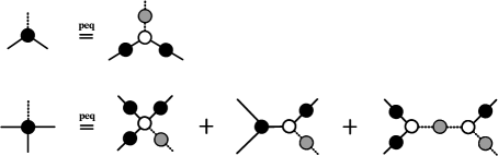
Figure 7: Diagrammatic representation for the partial equilibrium values of the correlators involving pressure fluctuation, as given by Eqs. (68). An open circle with $k$ legs represents the derivative of entropy with respect to $k$ variables, e.g., $S_{,mmp}$ for $k=3$, with solid and dashed lines representing derivatives with respect to $m$ and $p$, respectively. The solid gray circle with two dashed line legs represents $-S^{-1}_{,pp}=W^{\rm eq}_{pp}$, the equilibrium value of $W_{pp}$.

In order to check the validity of Eqs. (63)–(66) together with (68) we verified that they are solved by the following space-time and wave number independent values:

$$\begin{gathered}W_{mm}^{\rm eq}=\frac{m_{n}}{\alpha_{m}}\,,\quad W_{mp}^{\rm eq}=0\,,\quad W_{pp}^{\rm eq}=\frac{w}{\beta\epsilon_{p}}\,,\\[3.0pt] W_{mmm}^{\rm eq}=-\left(\frac{m_{n}}{\alpha_{m}}\right)^{2}\left(\frac{\alpha_{mm}}{\alpha_{m}}+\frac{4+2\alpha_{m}}{nm_{n}}-\frac{3\alpha_{p}}{\beta m_{n}}\right)\,,\quad W_{mmp}^{\rm eq}=-\frac{m_{n}}{\beta\alpha_{m}}\,,\\[3.0pt] W_{mmmm}^{\rm eq}=\left(\frac{m_{n}}{\alpha_{m}}\right)^{3}\bigg{[}-\frac{\alpha_{mmm}}{\alpha_{m}}+3\left(\frac{\alpha_{mm}}{\alpha_{m}}\right)^{2}+\frac{2\alpha_{mm}}{nm_{n}\alpha_{m}}\left(9+3\alpha_{m}-\frac{7n\alpha_{p}}{\beta}\right)+\frac{6\alpha_{mp}}{\beta m_{n}}+\frac{3\alpha_{m}\epsilon_{p}}{\beta wm_{n}}\\[2.0pt] ~{}~{}~{}~{}~{}~{}~{}~{}+\frac{3(2+\alpha_{m})(5+2\alpha_{m})}{n^{2}m_{n}^{2}}-\frac{\alpha_{p}}{\beta nm_{n}^{2}}\left(44+16\alpha_{m}-15\frac{n\alpha_{p}}{\beta}\right)\bigg{]}\,,\\[3.0pt] W_{mmmp}^{\rm eq}=\frac{2}{\beta}\left(\frac{m_{n}}{\alpha_{m}}\right)^{2}\left(\frac{\alpha_{mm}}{\alpha_{m}}+\frac{4+2\alpha_{m}}{nm_{n}}-\frac{3\alpha_{p}}{\beta m_{n}}\right)\,,\end{gathered}$$ (69)

which, of course, can be obtained from an independent calculation based on thermodynamics (see Appendix A). This is a highly nontrivial check of the evolution equations, since it involves cancellations of many terms, including the contribution of the pressure fluctuations discussed above.

Eqs. (69) are expressed in terms of independent thermodynamic derivatives from set I in Table 1. This is useful for verifying that equilibrium correlators in Eqs. (69) satisfy evolution equations. An alternative representation of Eqs. (69) using the independent thermodynamic derivatives from set II is given by Eqs. (84).

The terms involving $\theta$ reflect trivial expansion effect on the Wigner function described by the equation $u\cdot\partial W_{k}=(k-1)\theta W_{k}$. This effect was already discussed in Ref. An:2019fdc for $k=2$, where it was absorbed by rescaling $W_{k}$ by a factor of the density $n$ which also obeys a similar equation due to expansion: $u\cdot\partial n=-n\theta$. Generalizing this approach to arbitrary $k$ we can eliminate the terms with $\theta$ and simplify the expressions by writing the evolution equations in terms of rescaled Wigner functions $N$:

$$N_{\underbrace{{}_{m\dots m}}_{k}}=n^{k-1}W_{\underbrace{{}_{m\dots m}}_{k}}\,,\qquad N_{\underbrace{{}_{pm\dots m}}_{k}}=n^{k-1}W_{\underbrace{{}_{pm\dots m}}_{k}}\,.$$ (70)

In terms of $N$, equations (63) retain exactly the same form, but without $\theta$ terms (and with extra factor of $n$ for each $Q_{mm,m\dots}$, which is understandable recalling that $Q_{mm}$ is a two-point Wigner function), i.e.,

$$\mathcal{L}[N_{mm}(\bm{q}_{1},\bm{q}_{2})]= ~{}2\big{[}L_{m,m}(\bm{q}_{1},-\bm{q}_{1})N_{mm}(\bm{q}_{1},\bm{q}_{2})+nQ_{mm}(\bm{q}_{1},\bm{q}_{2})\big{]}_{\overline{12}}\,,$$ (71a)

$$\mathcal{L}[N_{mmm}(\bm{q}_{1},\bm{q}_{2},\bm{q}_{3})]= ~{}3\big{[}L_{m,m}(\bm{q}_{1},-\bm{q}_{1})N_{mmm}(\bm{q}_{1},\bm{q}_{2},\bm{q}_{3})$$

$$+L_{m,p}(\bm{q}_{1},-\bm{q}_{1})N_{pmm}(\bm{q}_{1},\bm{q}_{2},\bm{q}_{3})$$

$$+L_{m,mm}(\bm{q}_{1},\bm{q}_{2},\bm{q}_{3})N_{mm}(-\bm{q}_{2},\bm{q}_{2})N_{mm}(-\bm{q}_{3},\bm{q}_{3})$$

$$+2nQ_{mm,m}(\bm{q}_{1},\bm{q}_{2},\bm{q}_{3})N_{mm}(-\bm{q}_{3},\bm{q}_{3})\big{]}_{\overline{123}}\,,$$ (71b)

$$\mathcal{L}[N_{mmmm}(\bm{q}_{1},\bm{q}_{2},\bm{q}_{3},\bm{q}_{4})]= ~{}4\big{[}L_{m,m}(\bm{q}_{1},-\bm{q}_{1})N_{mmmm}(\bm{q}_{1},\bm{q}_{2},\bm{q}_{3},\bm{q}_{4})$$

$$+L_{m,p}(\bm{q}_{1},-\bm{q}_{1})N_{pmmm}(\bm{q}_{1},\bm{q}_{2},\bm{q}_{3},\bm{q}_{4})$$

$$+3L_{m,mm}(\bm{q}_{1},\bm{q}_{2},\bm{q}_{3}+\bm{q}_{4})N_{mm}(-\bm{q}_{2},\bm{q}_{2})N_{mmm}(-\bm{q}_{3}-\bm{q}_{4},\bm{q}_{3},\bm{q}_{4})$$

$$+3L_{m,mp}(\bm{q}_{1},\bm{q}_{2},\bm{q}_{3}+\bm{q}_{4})N_{mm}(-\bm{q}_{2},\bm{q}_{2})N_{pmm}(-\bm{q}_{3}-\bm{q}_{4},\bm{q}_{3},\bm{q}_{4})$$

$$+L_{m,mmm}(\bm{q}_{1},\bm{q}_{2},\bm{q}_{3},\bm{q}_{4})N_{mm}(-\bm{q}_{2},\bm{q}_{2})N_{mm}(-\bm{q}_{3},\bm{q}_{3})N_{mm}(-\bm{q}_{4},\bm{q}_{4})$$

$$+3nQ_{mm,m}(\bm{q}_{1},\bm{q}_{2},\bm{q}_{3}+\bm{q}_{4})N_{mmm}(-\bm{q}_{3}-\bm{q}_{4},\bm{q}_{3},\bm{q}_{4})$$

$$+3nQ_{mm,p}(\bm{q}_{1},\bm{q}_{2},\bm{q}_{3}+\bm{q}_{4})N_{pmm}(-\bm{q}_{3}-\bm{q}_{4},\bm{q}_{3},\bm{q}_{4})$$

$$+3nQ_{mm,mm}(\bm{q}_{1},\bm{q}_{2},\bm{q}_{3},\bm{q}_{4})N_{mm}(-\bm{q}_{3},\bm{q}_{3})N_{mm}(-\bm{q}_{4},\bm{q}_{4})\big{]}_{\overline{1234}}\,.$$ (71c)

The equilibrium solutions for Eqs. (71) can be obtained accordingly, using Eqs. (69) (or Eqs. (84)) and (70).

It is instructive to compare Eqs. (63) or (71) for fluctuations of $m$ to similar evolution equations for the fluctuations of $n$ at fixed $T$ in the charge diffusion problem derived in Ref. An_2021 . The following map between the two problems was conjectured in Ref. An_2021 (this substitution correctly reproduces the equation for the two-point correlator in Eq. (63a), already known from Ref. An:2019fdc ):

$$n\to m\,,\qquad\gamma\to\frac{\kappa}{c_{p}}\,,\qquad\alpha^{\prime}\to\frac{n^{2}}{c_{p}}\,.$$ (72)

While the substitution (72) reproduces the terms in Eqs. (63) or (71), the expressions for the coefficients in these equations given by Eqs. (65) contain terms with derivatives of $\ln m_{n}$ which are not reproduced by the simple map (72). These terms reflect the fact that the $\bm{q}=0$ mode of $n$, i.e., $\int\!d^{3}x\,n$, is a constant of motion, while $\int\!d^{3}x\,m$ is not (see Eq. (54)), unless $m$ happens to be a linear function of $n$, of course, in which case the derivatives of $\ln m_{n}$ vanish. Also, the contributions of the pressure fluctuations (the terms with $W_{pm\dots m}$) are not captured by the replacement in Eq. (72).

IV Conclusions and outlook

We have generalized the fully Lorentz covariant deterministic approach to relativistic fluctuating hydrodynamics to non-Gaussian fluctuations. While the full system of equations involving correlators of all hydrodynamic variables is still a work in progress, here we demonstrate how this approach allows us to derive the relativistically covariant equations for the fluctuations of the slowest hydrodynamic mode, which is specific entropy, or $m=s/n$, in a fluid with arbitrary relativistic flow. Such fluctuations are of special significance near a critical point, in particular, the QCD critical point, for two reasons. First, the equilibrium fluctuations of $m$ are the largest near the critical point: $\langle\delta m^{2}\rangle\sim c_{p}\sim\xi^{2-\eta}$. In that sense, this is the “soft” direction and the source of the most prominent critical point signatures. Second, this mode is also the slowest (not only it is diffusive, but its diffusion coefficient $\gamma_{\lambda}=\kappa/c_{p}$ vanishes at the critical point as $c_{p}$ diverges) and, thus, it is the furthest from equilibrium. Therefore, the non-equilibrium dynamics of this mode of fluctuations are the most consequential from the point of view of predicting the dynamical effects on the signatures of the QCD critical point.

Similar evolution equations for non-Gaussian correlators in a static (nonflowing) fluid at given temperature were derived in Ref. An_2021 . In this paper we consider diffusion of the slowest diffusive mode in a flowing fluid, more relevant for the description of the dynamics of critical fluctuations in heavy-ion collisions.

Comparing evolution equations (63) to the results of Ref. An_2021 we observe many similarities, which were already anticipated in Ref. An_2021 . In fact, equations (63) can be obtained from those in Ref. An_2021 by a substitution, Eq. (72), as conjectured in Ref. An_2021 . However, the terms containing derivatives of $\ln m_{n}$ appearing in the coefficients given by Eqs. (65) cannot be obtained that way. Their appearance is related to the qualitative difference between the density $n$, whose space integral is a conserved quantity, and the specific entropy $m$, whose space integral (i.e., $\bm{q}=0$ mode) is generally not conserved. We have also found nontrivial contributions of pressure fluctuations to the evolution of the specific entropy correlators due to non-linearities of the equation of state (i.e., mode coupling).

As a very nontrivial check of the evolution equations (63) and (65), we verified that the equilibrium (thermodynamic) correlators in Eq. (69) solve the evolution equations. This requires multiple cancellations which cannot be achieved without the terms with derivatives of $\ln m_{n}$ as well as the contributions of pressure fluctuations.

As we pointed out in the Introduction, our equations include only tree-level contributions (as did the equations derived in Ref. An_2021 ). It could potentially be interesting to extend this analysis to one-loop order and consider “long-time tail” effects on the evolution of fluctuations. The resulting theory would represent the generalization of Hydro+ Stephanov:2018hydro+ to non-Gaussian fluctuations.

Although we limited our analysis to the slowest diffusive mode, we presented our derivation in a sufficiently general form to facilitate the extension to fluctuations of faster hydrodynamic modes. The next-to-slowest modes correspond to fluctuations of the transverse velocity of the fluid. The theory describing fluctuations of all diffusive hydrodynamic modes (specific entropy and transverse velocity) was referred to as Hydro++ in Ref. An:2019fdc . Finally, the full set of hydrodynamic modes includes pressure/longitudinal velocity fluctuations, i.e., they include sound – the fastest hydrodynamic mode. We leave the development of such a full hydrodynamic theory of fluctuations to further work.

Despite the focus on the slowest hydrodynamic mode, we believe the equations presented in this paper are valuable for more realistic simulations of the dynamical evolution of fluctuations in heavy-ion collisions (as a first step one can consider extending exploratory Hydro+ calculations, such as in Refs. Rajagopal:2019hydro ; Du:2020bxp ; Pradeep:2022mkf , to non-Gaussian fluctuations). The ingredients required are the same as in the usual hydrodynamic simulation: equation of state, e.g., as in Refs. Parotto:2018pwx ; Karthein:2021nxe ; Kapusta:2021oco , and kinetic coefficients.

Appendix A Non-Gaussian correlators in thermodynamics

In the local rest frame, the total entropy subject to the conservation of charge and energy are given by

$$S(m,p)=\int_{\bm{x}}s(m,p)+\bar{\alpha}n(m,p)-\bar{\beta}\epsilon(m,p)\,,$$ (73)

where we choose our two independent thermodynamic variables as the specific entropy density $m$ and pressure $p$ associated with conserved quantities $n$ and $\epsilon$, i.e., $m=m(n,\epsilon)$, $p=p(n,\epsilon)$ and the variable associated with momentum (e.g., velocity $u$) is absent due to the fact that we choose the local rest frame. $\bar{\alpha}$ and $\bar{\beta}$ are the local chemical potential per temperature and inverse of temperature of the heat bath respectively.

For a system with two independent thermodynamic variables (such as $m$ and $p$), there are $n+1$ independent $n$th-order thermodynamic derivatives of entropy. It is convenient for calculations to choose a basis set of independent derivatives for each order to make sure that cancellations are easier to carry out. Table 1 provides two such basis sets (set I and II) for derivatives up to fourth order. In set I and II we have primarily chosen the derivatives of $\alpha$ and $\ln m_{n}$, respectively. Of course, one can relate the independent thermodynamic derivatives from set I to those from set II. Taking the second-order derivative as an example, we have

$$\begin{gathered}\epsilon_{p}=2+\alpha_{m}+nm_{n}(\ln m_{n})_{,m}-w(\ln m_{n})_{,p}\,,\qquad\alpha_{p}=\beta m_{n}(\ln m_{n})_{,m}+\frac{\beta}{n}(2+\alpha_{m})\,,\end{gathered}$$ (74)

while $\alpha_{m}$ and $m_{n}/\alpha_{m}$ are simply functions of each other and the first-order derivative $m_{n}=-\beta w/n^{2}$, so we can also treat $\alpha_{m}$ instead of $m_{n}/\alpha_{m}$ as an independent thermodynamic derivative in set II.

order	independent derivatives (set I)	independent derivatives (set II)
2nd	$\epsilon_{p},\,\alpha_{m},\,\alpha_{p}$	$\frac{m_{n}}{\alpha_{m}},\,(\ln m_{n})_{,m},\,(\ln m_{n})_{,p}$
3rd	$\epsilon_{pp},\,\alpha_{mm},\,\alpha_{mp},\,\alpha_{pp}$	$\left(\ln\frac{m_{n}}{\alpha_{m}}\right)_{,m},\,(\ln m_{n})_{,mm},\,(\ln m_{n})_{,mp},\,(\ln m_{n})_{,pp}$
4th	$\epsilon_{ppp},\,\alpha_{mmm},\,\alpha_{mmp},\,\alpha_{mpp},\,\alpha_{ppp}$	$\left(\ln\frac{m_{n}}{\alpha_{m}}\right)_{,mm},\,(\ln m_{n})_{,mmm},\,(\ln m_{n})_{,mmp},\,(\ln m_{n})_{,mpp},\,(\ln m_{n})_{,ppp}$

Table 1: Two sets of independent thermodynamic derivatives chosen in this work. The derivative of quantity $X$ with respect to $m$ (or $p$) while keeping $p$ (or $m$) fixed is denoted by $X_{m}$ (or $X_{p}$).

As a consequence, all thermodynamic derivatives can be expressed solely in terms of the independent ones such as those listed in Table 1. In terms of the independent derivatives from set I given by Table 1, useful expressions for some second-, third-, and fourth-order thermodynamic derivatives are presented below:

$$\begin{gathered}n_{m}=\frac{1}{m_{n}}\left(1-\frac{n\alpha_{p}}{\beta}\right)\,,\quad n_{p}=\frac{n\epsilon_{p}}{w}\,,\quad\epsilon_{m}=-\frac{w\alpha_{p}}{\beta m_{n}}\,,\quad\beta_{m}=\frac{n\alpha_{m}}{w}\,,\quad\beta_{p}=-\frac{\beta}{w}\left(1-\frac{n\alpha_{p}}{\beta}\right)\,,\\[4.0pt] n_{mm}=\frac{1}{m_{n}}\left[-\frac{n\alpha_{mp}}{\beta}+\frac{2n\alpha_{p}^{2}}{\beta^{2}m_{n}}+\frac{2+\alpha_{m}}{nm_{n}}\left(1-\frac{2n\alpha_{p}}{\beta}\right)\right]\,,\quad n_{pp}=-\frac{n}{w^{2}}\left(w\epsilon_{pp}-\epsilon_{p}\right)\,,\\[4.0pt] \epsilon_{mm}=-\frac{w\alpha_{p}}{\beta m_{n}}\left[\frac{\alpha_{mp}}{\alpha_{p}}+\frac{2}{nm_{n}}\left(1+\alpha_{m}-\frac{n\alpha_{p}}{\beta}\right)\right]\,,\quad\epsilon_{mp}=-\frac{\alpha_{p}}{\beta m_{n}}\left[\frac{w\alpha_{pp}}{\alpha_{p}}+2\left(1+\epsilon_{p}-\frac{n\alpha_{p}}{\beta}\right)\right]\,,\\[4.0pt] n_{mmm}=\frac{1}{m_{n}}\Bigg{[}-\frac{n\alpha_{mmp}}{\beta}+\frac{\alpha_{mm}}{nm_{n}}\left(1-\frac{2n\alpha_{p}}{\beta}\right)-\frac{\alpha_{mp}}{\beta m_{n}}\left(7+4\alpha_{m}-\frac{6n\alpha_{p}}{\beta}\right)~{}~{}~{}~{}~{}~{}~{}~{}~{}~{}~{}~{}~{}~{}~{}~{}~{}~{}\\ ~{}~{}~{}~{}~{}~{}~{}~{}~{}~{}~{}~{}~{}~{}~{}~{}+6\left(\frac{\alpha_{p}}{\beta m_{n}}\right)^{2}\left(3+2\alpha_{m}-\frac{n\alpha_{p}}{\beta}\right)+\frac{(2+\alpha_{m})(3+2\alpha_{m})}{n^{2}m_{n}^{2}}\left(1-\frac{3\alpha_{p}n}{\beta}\right)\Bigg{]}\,,\\[4.0pt] \epsilon_{mmm}=-\frac{w\alpha_{p}}{\beta m_{n}}\left[\frac{\alpha_{mmp}}{\alpha_{p}}+\frac{2\alpha_{mp}}{nm_{n}\alpha_{p}}\left(2+2\alpha_{m}-\frac{3n\alpha_{p}}{\beta}\right)+6\left(1+\alpha_{m}-\frac{\alpha_{p}}{\beta m_{n}}\right)^{2}\right]\,.\end{gathered}$$ (75)

Applying the derivative with respect to $m$ or $p$ to the entropy given by Eq. (73), we obtain

$$\begin{gathered}S_{,\,m}=0\,,\quad S_{,\,p}=0\,,\quad S_{,\,mm}=-\frac{\alpha_{m}}{m_{n}}\,,\quad S_{,\,mp}=0\,,\quad S_{,\,pp}=-\frac{\beta\epsilon_{p}}{w}\,,\quad S_{,\,mmp}=-\frac{\alpha_{m}\epsilon_{p}}{wm_{n}}\,,\\[3.0pt] S_{,\,mmm}=-\frac{\alpha_{m}}{m_{n}}\left(\frac{\alpha_{mm}}{\alpha_{m}}+\frac{2(2+\alpha_{m})}{nm_{n}}-\frac{3\alpha_{p}}{\beta m_{n}}\right),\quad S_{,\,mpp}=\frac{\alpha_{p}}{wm_{n}}\left(\frac{w\alpha_{pp}}{\alpha_{p}}-\frac{2n\alpha_{p}}{\beta}+\epsilon_{p}+2\right)\,,\\[3.0pt] S_{,\,mmmp}=\frac{\alpha_{m}}{m_{n}}\left[\frac{3\alpha_{pp}}{\beta m_{n}}-\left(\frac{\alpha_{mm}}{\alpha_{m}}+\frac{2+\alpha_{m}}{nm_{n}}-\frac{6\alpha_{p}}{\beta m_{n}}\right)\frac{\epsilon_{p}}{w}+\frac{6\alpha_{p}}{\beta wm_{n}}\left(1-\frac{n\alpha_{p}}{\beta}\right)\right]\,,\\[3.0pt] S_{,\,\,mmmm}=-\frac{\alpha_{m}}{m_{n}}\bigg{[}\frac{\alpha_{mmm}}{\alpha_{m}}+\frac{2\alpha_{mm}}{nm_{n}\alpha_{m}}\left(3+3\alpha_{m}-\frac{2n\alpha_{p}}{\beta}\right)-\frac{6\alpha_{mp}}{\beta m_{n}}+\frac{3(2+\alpha_{m})(3+2\alpha_{m})}{n^{2}m_{n}^{2}}\\[2.0pt] -\frac{4\alpha_{p}}{\beta nm_{n}^{2}}\left(7+5\alpha_{m}-\frac{3n\alpha_{p}}{\beta}\right)\bigg{]}\,.\end{gathered}$$ (76)

The above expressions for entropy derivatives are evaluated at the maximum of the entropy $S$ (i.e., in equilibrium), which corresponds to $\alpha=\bar{\alpha}$ and $\beta=\bar{\beta}$. As in Ref. An:2019rhf ; An:2019fdc , the choice of $m$ and $p$ as independent thermodynamic variables makes the second-order entropy derivative quadratic form diagonal, i.e., $S_{,mp}=0$.

The connected $n$-point correlation functions in thermodynamic equilibrium are given by

$$\begin{gathered}W^{\rm eq}_{i_{1}i_{2}}=-S^{-1}_{,\,i_{1}i_{2}}\,,\quad W^{\rm eq}_{i_{1}i_{2}i_{3}}=-S^{-1}_{,\,i_{1}j_{1}}S^{-1}_{,\,i_{2}j_{2}}S^{-1}_{,\,i_{3}j_{3}}S_{,\,j_{1}j_{2}j_{3}}\,,\\ W^{\rm eq}_{i_{1}i_{2}i_{3}i_{4}}=\bigg{[}S^{-1}_{,\,i_{1}j_{1}}S^{-1}_{,\,i_{2}j_{2}}S^{-1}_{,\,i_{3}j_{3}}S^{-1}_{,\,i_{4}j_{4}}S_{,\,j_{1}j_{2}j_{3}j_{4}}-3S^{-1}_{,\,i_{1}j_{1}}S^{-1}_{,\,i_{2}j_{2}}S_{,\,j_{1}j_{2}j_{3}}S^{-1}_{,\,j_{3}j_{4}}S_{,\,j_{4}j_{5}j_{6}}S^{-1}_{,\,j_{5}i_{3}}S^{-1}_{,\,j_{6}j_{4}}\bigg{]}_{\overline{i_{1}i_{2}i_{3}i_{4}}}\,,\end{gathered}$$ (77)

and generically

$$W^{\rm eq}_{i_{1}\dots i_{n}}=\bigg{[}W^{\rm eq}_{i_{1}j_{1}}W^{\rm eq}_{i_{2}\dots i_{n},\,j_{1}}\bigg{]}_{\overline{i_{1}\dots i_{n}}}\,,$$ (78)

where indices $i_{n}$’s label the external points while indices $j_{n}$’s label the internal ones. The relation given by Eq. (78) easily follows from the cumulant generating function $g_{\rm c}(\mu_{1},\dots,\mu_{n})$ such that $W^{\rm eq}_{i_{1}\dots i_{n}}=d^{n}g_{\rm c}/d\mu_{1}\dots d\mu_{n}$. Indeed, using the chain rule on the $\mu$ derivative in $W^{\rm eq}_{i_{1}\dots i_{n}}=\left[dW^{\rm eq}_{i_{2}\dots i_{n}}/d\mu_{1}\right]_{\overline{1\dots n}}$ and the fact that (susceptibility) $d\psi_{j}/d\mu_{i}=W^{\rm eq}_{ij}$ we obtain Eq. (78).

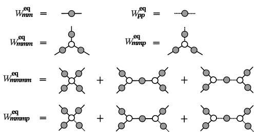
Figure 8: Diagrammatic representation of the equilibrium correlation functions in Eq. (79). A solid (dashed) line entering a vertex denotes the $m$ ($p$) index. Open circles represent entropy derivatives. The solid gray circles with two legs are equilibrium two-point correlators expressed in terms of the second derivatives of the entropy: $W^{\rm eq}_{mm}=-S^{-1}_{mm}$ and $W^{\rm eq}_{pp}=-S^{-1}_{pp}$. Note the absence of the cross-correlator $W^{\rm eq}_{mp}=0$, which simplifies the calculation.

In the discussion presented in Sec. III, the indices are chosen as $i\text{'s}=m$ and $j\text{'s}=(m,p)$, thus the connected $n$-point functions are (see Fig. 8 for diagrammatic representation)

$$\begin{gathered}W^{\rm eq}_{mm}=-S^{-1}_{,\,mm}\,,\quad W^{\rm eq}_{mp}=0\,,\quad W^{\rm eq}_{pp}=-S^{-1}_{,\,pp}\,,\\[3.0pt] W^{\rm eq}_{mmm}=-S^{-3}_{,\,mm}S_{,\,mmm}\,,\quad W^{\rm eq}_{mmp}=-S^{-2}_{,\,mm}S^{-1}_{pp}S_{,\,mmp}\,,\\[3.0pt] W^{\rm eq}_{mmmm}=S^{-4}_{,\,mm}S_{,\,mmmm}-3S^{-5}_{,\,mm}(S_{,\,mmm})^{2}-3S^{-4}_{,\,mm}S^{-1}_{,\,pp}(S_{,\,mmp})^{2}\,,\\[3.0pt] W^{\rm eq}_{mmmp}=S^{-3}_{,\,mm}S^{-1}_{,\,pp}S_{,\,mmmp}-3S^{-4}_{,\,mm}S^{-1}_{,\,pp}S_{,\,mmm}S_{,\,mmp}-3S^{-3}_{,\,mm}S^{-2}_{,\,pp}S_{,\,mmp}S_{,\,mpp}\,,\end{gathered}$$ (79)

where we have used the fact that $S_{,mp}=0$ given in Eq. (76), which largely simplifies our calculation. Now substituting Eq. (76) into Eq. (79) one immediately obtains Eq. (69).

Interestingly, one can infer the following relations from the above expressions:

$$\begin{gathered}W_{mmp}^{\rm eq}=-\frac{1}{\beta}W_{mm}^{\rm eq}\,,\quad W_{mmmp}^{\rm eq}=-\frac{2}{\beta}W_{mmm}^{\rm eq}\,.\end{gathered}$$ (80)

The above relations, similarly to $W_{mp}^{\rm eq}=0$, are consequences of choosing $m$ and $p$ as our independent thermodynamic variables.

Appendix B Partial equilibrium for pressure fluctuations

We shall now use the equilibrium entropy functional given by Eq. (73) to determine the partial equilibrium value of $\delta p$. This value, $(\delta p)^{\rm peq}$, maximizes the entropy functional $S$ under the condition that $\delta m$ is fixed. Thus, $(\delta p)^{\rm peq}$ is determined by solving $S_{,p}(m+\delta m,p+(\delta p)^{\rm peq})=0$, were $m$ and $p$ are full equilibrium values, determined by $S_{,m}(m,p)=S_{,p}(m,p)=0$. As a result we obtain

$$(\delta p)^{\rm peq}=\,-\frac{1}{2}S_{,pp}^{-1}S_{,mmp}\delta m^{2}-\left(\frac{1}{6}S_{,pp}^{-1}S_{,mmmp}-\frac{1}{2}S_{,pp}^{-2}S_{,mmp}S_{,mpp}\right)\delta m^{3}\,,$$ (81)

where we truncated the solution to the order we need to calculate the third and fourth order correlators. Notice, that the absence of a term linear in $\delta m$ is a consequence of the well-known fact that the fluctuations of pressure and specific entropy are not correlated, or $S_{,mp}=0$. This lack of correlation, however, does not persist beyond the linear order. This observation is important for the non-Gaussian fluctuation equations we derive in this paper.

Using Eq. (81), we can now calculate partial equilibrium values of the cross-correlators of pressure and specific entropy, such as

$$G^{\rm c,peq}_{pmm}(x_{1},x_{2},x_{3})\equiv \,\langle{:\!(\delta p)^{\rm peq}(x_{1})\!:\delta m(x_{2})\delta m(x_{3})}\rangle_{\rm c}=-\frac{1}{2}S_{,pp}^{-1}S_{,mmp}\langle{:\!\delta m(x_{1})^{2}\!:\delta m(x_{2})\delta m(x_{3})}\rangle_{\rm c}$$

$$= -S_{,pp}^{-1}S_{,mmp}G^{\rm c}_{mm}(x_{1},x_{2})G^{\rm c}_{mm}(x_{1},x_{3})\,,$$

$$G^{\rm c,peq}_{pmmm}(x_{1},x_{2},x_{3},x_{4})\equiv \,\langle{:\!(\delta p)^{\rm peq}(x_{1})\!:\delta m(x_{2})\delta m(x_{3})\delta m(x_{4})}\rangle_{\rm c}$$

$$= -\frac{1}{2}S_{,pp}^{-1}S_{,mmp}\langle{:\delta m(x_{1})^{2}:\delta m(x_{2})\delta m(x_{3})\delta m(x_{4})}\rangle_{\rm c}$$

$$-\left(\frac{1}{6}S_{,pp}^{-1}S_{,mmmp}-\frac{1}{2}S_{,pp}^{-2}S_{,mmp}S_{,mpp}\right)\langle{:\!\delta m(x_{1})^{3}\!:\delta m(x_{2})\delta m(x_{3})\delta m(x_{4})}\rangle_{\rm c}$$

$$= -3S_{,pp}^{-1}S_{,mmp}G^{\rm c}_{mm}(x_{1},x_{2})G^{\rm c}_{mmm}(x_{1},x_{3},x_{4})$$

$$-\left(S_{,pp}^{-1}S_{,mmmp}-3S_{,pp}^{-2}S_{,mmp}S_{,mpp}\right)G^{\rm c}_{mm}(x_{1},x_{2})G^{\rm c}_{mm}(x_{1},x_{3})G^{\rm c}_{mm}(x_{1},x_{4})|_{\overline{x_{2}x_{3}x_{4}}}\,,$$

where in the second equality of each above equation, we neglected the terms which contribute to higher order in fluctuation expansion parameter $\varepsilon$. Finally, taking the $n$-point Wigner transform (41), we obtain Eqs. (68).

Appendix C Alternative expressions in terms of independent thermodynamic derivatives

We have expressed Eqs. (66) and (69) in terms of the independent thermodynamic derivatives chosen from set I given by Table 1. There are, of course, numerous different choices for the independent thermodynamic derivatives in terms of which our equations can be formulated. In this section we provide alternative expressions for these equations, which are instead expressed in terms of independent thermodynamic derivatives specified in set II, where all independent derivatives of $\ln m_{n}$ (with respect to $m$ or $p$) are chosen as the independent thermodynamic derivatives.

The presence of the derivatives of $m_{n}$ reflects the fact that the volume integral of $m$ is not a constant of motion, in contrast to the volume integral of $n$. The choice of the independent thermodynamic derivatives given by set II allows us to quantify such a difference. For example, if $m$ were to be a linear function of $n$, $m_{n}$ would be a constant and all thermodynamic derivatives acting on $m_{n}$ would vanish, significantly simplifying above equations. In this case, there is only one independent $n$th-order thermodynamic derivative (cf. Table 1), as in the charge diffusion problem studied in Ref. An_2021 .

The alternative expressions for Eqs. (66), in terms of the independent thermodynamic derivatives from set II, read

$$\begin{gathered}\gamma_{mm}=m_{n}\lambda\alpha_{m}\,,\qquad\gamma_{mp}=\left(\frac{2+\alpha_{m}}{nm_{n}}+(\ln m_{n})_{,m}\right)\beta m_{n}^{2}\lambda\,,\\[4.0pt] (\gamma_{mm})_{,m}=\Bigg{(}(\ln\lambda)_{,m}+2(\ln m_{n})_{,m}-\left(\ln\frac{m_{n}}{\alpha_{m}}\right)_{,m}\Bigg{)}\gamma_{mm}\,,\\[4.0pt] (\gamma_{mm})_{,p}=\bigg{[}(\ln m_{n})_{,mm}-\frac{\alpha_{m}}{nm_{n}}\left(\ln\frac{m_{n}}{\alpha_{m}}\right)_{,m}+\left(\frac{2+\alpha_{m}}{nm_{n}}+(\ln m_{n})_{,m}\right)(\ln m_{n})_{,m}\\[2.0pt] +\frac{\alpha_{m}}{\beta m_{n}}\left((\ln\lambda)_{,p}+(\ln m_{n})_{,p}\right)+\frac{2+\alpha_{m}}{n^{2}m_{n}^{2}}\bigg{]}\beta m_{n}^{2}\lambda\,,\\[4.0pt] (\gamma_{mp})_{,m}=\bigg{[}(\ln m_{n})_{,mm}-\frac{\alpha_{m}}{nm_{n}}\left(\ln\frac{m_{n}}{\alpha_{m}}\right)_{,m}\\[2.0pt] +\left(\frac{2+\alpha_{m}}{nm_{n}}+(\ln m_{n})_{,m}\right)\left((\ln\lambda)_{,m}+2(\ln m_{n})_{,m}\right)+\frac{2+\alpha_{m}}{n^{2}m_{n}^{2}}\bigg{]}\beta m_{n}^{2}\lambda\,,\\[4.0pt] (\gamma_{mm})_{,mm}=\Bigg{[}(\ln\lambda)_{,mm}+2(\ln m_{n})_{,mm}-\left(\ln\frac{m_{n}}{\alpha_{m}}\right)_{,mm}\\[2.0pt] +\left((\ln\lambda)_{,m}+2(\ln m_{n})_{,m}-\left(\ln\frac{m_{n}}{\alpha_{m}}\right)_{,m}\right)^{2}\Bigg{]}\gamma_{mm}\,,\\[6.0pt] (m_{n}^{2}\lambda)_{,m}=\left((\ln\lambda)_{,m}+2(\ln m_{n})_{,m}\right)m_{n}^{2}\lambda\,,\qquad(m_{n}^{2}\lambda)_{,p}=\left((\ln\lambda)_{,p}+2(\ln m_{n})_{,p}\right)m_{n}^{2}\lambda\,,\\[8.0pt] (m_{n}p_{n}\lambda)_{,m}=\left((\ln\lambda)_{,m}+(\ln m_{n})_{,m}+(\ln p_{n})_{,m}\right)m_{n}p_{n}\lambda\,,\\[4.0pt] p_{n}=\frac{w}{n}-\frac{w}{\beta}(\ln m_{n})_{,p}\left((\ln m_{n})_{,m}+\frac{n(\ln m_{n})_{,p}}{\beta}+\frac{2+\alpha_{m}}{nm_{n}}\right)^{-1}\,,\\[4.0pt] (\ln p_{n})_{,m}=-\frac{2}{nm_{n}}+\frac{nm_{n}(\ln m_{n})_{,mm}-\alpha_{m}\left(\ln\frac{m_{n}}{\alpha_{m}}\right)_{,m}+\frac{2+\alpha_{m}}{nm_{n}}}{nm_{n}(\ln m_{n})_{,m}+2+\alpha_{m}}\\[2.0pt] +\frac{\alpha_{m}\left(\ln\frac{m_{n}}{\alpha_{m}}\right)_{,m}-nm_{n}(\ln m_{n})_{,mm}+w(\ln m_{n})_{,mp}-w(\ln m_{n})_{,p}\left((\ln m_{n})_{,m}+\frac{2+\alpha_{m}}{nm_{n}}\right)+(\ln m_{n})_{,m}}{nm_{n}(\ln m_{n})_{,m}-w(\ln m_{n})_{,p}+2+\alpha_{m}}\,,\\[4.0pt] (m_{n}^{2}\lambda)_{,mm}=\left((\ln\lambda)_{,mm}+2(\ln m_{n})_{,mm}+((\ln\lambda)_{,m}+2(\ln m_{n})_{,m})^{2}\right)m_{n}^{2}\lambda\,.\end{gathered}$$ (83)

Note again that we also treat $\alpha_{m}$ as an independent second-order thermodynamic derivative as $m_{n}/\alpha_{m}$, since they are different by $m_{n}=-\beta w/n^{2}$ which is only a first-order thermodynamic derivative.

The alternative expressions for Eqs. (69) likewise read

$$\begin{gathered}W_{mm}^{\rm eq}=\frac{m_{n}}{\alpha_{m}}\,,\quad W_{mp}^{\rm eq}=0\,,\quad W_{pp}^{\rm eq}=-\frac{n}{\beta^{2}}\left(\frac{2+\alpha_{m}}{nm_{n}}+(\ln m_{n})_{,m}-\frac{w}{nm_{n}}(\ln m_{n})_{,p}\right)^{-1}\,,\\ W_{mmm}^{\rm eq}=\left(\frac{m_{n}}{\alpha_{m}}\right)^{2}\left[\left(\ln\frac{m_{n}}{\alpha_{m}}\right)_{,m}+2(\ln m_{n})_{,m}+\frac{2+\alpha_{m}}{nm_{n}}\right]\,,\quad W_{mmp}^{\rm eq}=-\frac{m_{n}}{\beta\alpha_{m}}\,,\\ W_{mmmm}^{\rm eq}=\left(\frac{m_{n}}{\alpha_{m}}\right)^{3}\Bigg{[}\left(\ln\frac{m_{n}}{\alpha_{m}}\right)_{,mm}+2\left(\left(\ln\frac{m_{n}}{\alpha_{m}}\right)_{,m}+5(\ln m_{n})_{,m}+\frac{5+\alpha_{m}}{nm_{n}}\right)\left(\ln\frac{m_{n}}{\alpha_{m}}\right)_{,m}\\ +5(\ln m_{n})_{,mm}+9\left((\ln m_{n})_{,m}+\frac{2+\alpha_{m}}{nm_{n}}\right)(\ln m_{n})_{,m}-\frac{3\alpha_{m}}{\beta m_{n}}(\ln m_{n})_{,p}+\frac{(2+\alpha_{m})(7+2\alpha_{m})}{n^{2}m_{n}^{2}}\Bigg{]}\,,\\ W_{mmmp}^{\rm eq}=-\frac{2}{\beta}\left(\frac{m_{n}}{\alpha_{m}}\right)^{2}\left[\left(\ln\frac{m_{n}}{\alpha_{m}}\right)_{,m}+2(\ln m_{n})_{,m}+\frac{2+\alpha_{m}}{nm_{n}}\right]\,.\end{gathered}$$ (84)

Appendix D Notations

This appendix summarizes the notations introduced in Section II.4.

• $\bar{\nabla}_{\mu}$ – confluent derivative – Eqs. (31), (45);

• $\bar{\omega}^{\nu}_{\lambda\mu}$ – confluent connection – Eq. (28);

• $\mathring{\omega}^{a}_{\mu b}$ – spin connection for local triad $e^{a}$ – Eq. (37), Fig. 4;

• $\mathring{\partial}_{\mu}G_{n}(x_{1},\ldots,x_{n})$ – derivative with respect to the midpoint $x$ at fixed $y_{i}^{a}$ – Eq. (35);

• $\bar{\nabla}_{\mu}{\bar{G}}_{n}$ – confluent derivative of ${\bar{G}}_{n}$ – Eq. (31);

• $G_{n}\equiv G_{i_{1}\dots i_{n}}$ – “raw” $n$-point correlator – Eq. (9);

• $G_{n}^{\text{c}}\equiv G_{i_{1}\dots i_{n}}^{\text{c}}$ – connected $n$-point correlator – Eqs. (15), (17), (20);

• ${\bar{G}}_{n}\equiv{\bar{G}}_{i_{1}\dots i_{n}}$ – confluent correlator – Eq. (II.4), Fig. 3;

• $W_{n}\equiv W_{i_{1}\dots i_{n}}$ – Wigner transform of connected confluent correlator ${\bar{G}}_{n}^{\text{c}}$ – Eq. (41);

• $\mathring{\partial}_{\mu}{W}_{n}(x;\bm{q}_{1},\ldots,\bm{q}_{n})$ – partial $x$-derivative at fixed $\bm{q}_{i}$’s (Wigner transform of $\mathring{\partial}_{\mu}{\bar{G}}_{n}^{\text{c}}$) – Eq. (43);

• $\bar{\nabla}_{\mu}{W}_{n}$ – confluent derivative of $W_{n}$ (Wigner transform of $\bar{\nabla}_{\mu}{\bar{G}}_{n}^{\text{c}}$) – Eq. (45);

• $x$ – the midpoint space-time vector – Eq.(26);

• $y_{i}\equiv x_{i}-x$ – the separation four-vector – Eq. (30);

• $y_{i}^{a}\equiv e^{a}\cdot y_{i}$ – the components of the separation vector in the local triad basis $e^{a}(x)$, $a=1,2,3$.

References

- (1) L. Landau and E. Lifshitz, Statistical Physics, Part 2, vol. 9 of Course of Theoretical Physics. Elsevier Science, 2013.
- (2) L. Landau and E. Lifshitz, Fluid Mechanics, vol. 6 of Course of Theoretical Physics. Elsevier Science, 2013.
- (3) S. Jeon and U. Heinz, “Introduction to Hydrodynamics,” Int. J. Mod. Phys. E 24 no. 10, (2015) 1530010, arXiv:1503.03931 [hep-ph].
- (4) P. Romatschke and U. Romatschke, Relativistic Fluid Dynamics In and Out of Equilibrium – Ten Years of Progress in Theory and Numerical Simulations of Nuclear Collisions. Cambridge University Press, 2019. arXiv:1712.05815 [nucl-th].
- (5) STAR Collaboration, M. M. Aggarwal et al., “An Experimental Exploration of the QCD Phase Diagram: The Search for the Critical Point and the Onset of De-confinement,” arXiv:1007.2613 [nucl-ex].
- (6) M. Stephanov, K. Rajagopal, and E. Shuryak, “Signatures of the tricritical point in QCD,” Phys.Rev.Lett. 81 (1998) 4816–4819, arXiv:hep-ph/9806219 [hep-ph].
- (7) M. Stephanov, K. Rajagopal, and E. Shuryak, “Event-by-event fluctuations in heavy ion collisions and the QCD critical point,” Phys. Rev. D 60 (1999) 114028, arXiv:hep-ph/9903292.
- (8) M. Stephanov, “QCD phase diagram and the critical point,” Prog. Theor. Phys. Suppl. 153 (2004) 139–156, arXiv:hep-ph/0402115.
- (9) A. Bzdak, S. Esumi, V. Koch, J. Liao, M. Stephanov, and N. Xu, “Mapping the Phases of Quantum Chromodynamics with Beam Energy Scan,” arXiv:1906.00936 [nucl-th].
- (10) X. An et al., “The BEST framework for the search for the QCD critical point and the chiral magnetic effect,” Nucl. Phys. A 1017 (2022) 122343, arXiv:2108.13867 [nucl-th].
- (11) M. Stephanov, “Non-Gaussian fluctuations near the QCD critical point,” Phys. Rev. Lett. 102 (2009) 032301, arXiv:0809.3450 [hep-ph].
- (12) M. Stephanov, “On the sign of kurtosis near the QCD critical point,” Phys. Rev. Lett. 107 (2011) 052301, arXiv:1104.1627 [hep-ph].
- (13) STAR Collaboration, M. Abdallah et al., “Cumulants and correlation functions of net-proton, proton, and antiproton multiplicity distributions in Au+Au collisions at energies available at the BNL Relativistic Heavy Ion Collider,” Phys. Rev. C 104 no. 2, (2021) 024902, arXiv:2101.12413 [nucl-ex].
- (14) B. Berdnikov and K. Rajagopal, “Slowing out-of-equilibrium near the QCD critical point,” Phys. Rev. D 61 (2000) 105017, arXiv:hep-ph/9912274 [hep-ph].
- (15) S. Mukherjee, R. Venugopalan, and Y. Yin, “Real time evolution of non-Gaussian cumulants in the QCD critical regime,” Phys. Rev. C 92 (2015) 034912, arXiv:1506.00645 [hep-ph].
- (16) Y. Akamatsu, A. Mazeliauskas, and D. Teaney, “Kinetic regime of hydrodynamic fluctuations and long time tails for a bjorken expansion,” Phys. Rev. C 95 (Jan, 2017) 014909.
- (17) Y. Akamatsu, A. Mazeliauskas, and D. Teaney, “Bulk viscosity from hydrodynamic fluctuations with relativistic hydrokinetic theory,” Phys. Rev. C 97 (Feb, 2018) 024902.
- (18) M. Martinez and T. Schäfer, “Stochastic hydrodynamics and long time tails of an expanding conformal charged fluid,” Phys. Rev. C 99 no. 5, (2019) 054902, arXiv:1812.05279 [hep-th].
- (19) X. An, G. Başar, M. Stephanov, and H.-U. Yee, “Relativistic Hydrodynamic Fluctuations,” Phys. Rev. C 100 (2019) 024910, arXiv:1902.09517 [hep-th].
- (20) X. An, G. Başar, M. Stephanov, and H.-U. Yee, “Fluctuation dynamics in a relativistic fluid with a critical point,” Phys. Rev. C 102 (2020) 034901, arXiv:1912.13456 [hep-th].
- (21) X. An, “Relativistic dynamics of fluctuations and QCD critical point,” Nucl. Phys. A 1005 (2021) 121957, arXiv:2003.02828 [hep-th].
- (22) X. An, G. Başar, M. Stephanov, and H.-U. Yee, “Evolution of non-gaussian hydrodynamic fluctuations,” Phys. Rev. Lett. 127 (2021) 072301, arXiv:2009.10742 [hep-th].
- (23) X. An, “Non-gaussian fluctuation dynamics,” Acta Phys. Pol. B Proc. Suppl. 16 (2023) 1–A47, arXiv:2209.15005 [hep-th].
- (24) A. Andreev, “Two-liquid effects in a normal liquid,” Zh. Ehksp. Teor. Fiz. 59 (1970) 1819–1827.
- (25) A. Andreev, “Corrections to the hydrodynamics of liquids,” Zh. Ehksp. Teor. Fiz. 75 no. 3, (1978) 1132–1139.
- (26) S. Mukherjee, R. Venugopalan, and Y. Yin, “Universal off-equilibrium scaling of critical cumulants in the QCD phase diagram,” Phys. Rev. Lett. 117 no. 22, (2016) 222301, arXiv:1605.09341 [hep-ph].
- (27) M. Nahrgang, M. Bluhm, T. Schaefer, and S. A. Bass, “Diffusive dynamics of critical fluctuations near the QCD critical point,” Phys. Rev. D 99 no. 11, (2019) 116015, arXiv:1804.05728 [nucl-th].
- (28) N. Sogabe and Y. Yin, “Off-equilibrium non-Gaussian fluctuations near the QCD critical point: an effective field theory perspective,” JHEP 03 (2022) 124, arXiv:2111.14667 [nucl-th].
- (29) M. Stephanov and Y. Yin, “Hydrodynamics with parametric slowing down and fluctuations near the critical point,” Phys. Rev. D 98 (Aug, 2018) 036006.
- (30) P. Hohenberg and B. Halperin, “Theory of dynamic critical phenomena,” Rev. Mod. Phys. 49 (Jul, 1977) 435–479.
- (31) M. S. Pradeep and M. Stephanov, “Maximum entropy freezeout of hydrodynamic fluctuations,” arXiv:2211.09142 [hep-ph].
- (32) STAR Collaboration, “Beam Energy Dependence of Fifth and Sixth-Order Net-proton Number Fluctuations in Au+Au Collisions at RHIC,” Phys. Rev. Lett. 130 (7, 2023) 082301, arXiv:2207.09837 [nucl-ex].
- (33) J. I. Kapusta, B. Muller, and M. Stephanov, “Relativistic Theory of Hydrodynamic Fluctuations with Applications to Heavy Ion Collisions,” Phys. Rev. C 85 (2012) 054906, arXiv:1112.6405 [nucl-th].
- (34) K. Rajagopal, G. Ridgway, R. Weller, and Y. Yin, “Understanding the out-of-equilibrium dynamics near a critical point in the qcd phase diagram,” Phys. Rev. D 102 (Nov, 2020) 094025, arXiv:1908.08539 [hep-ph].
- (35) L. Du, U. Heinz, K. Rajagopal, and Y. Yin, “Fluctuation dynamics near the QCD critical point,” Phys. Rev. C 102 no. 5, (2020) 054911, arXiv:2004.02719 [nucl-th].
- (36) M. Pradeep, K. Rajagopal, M. Stephanov, and Y. Yin, “Freezing out fluctuations in Hydro+ near the QCD critical point,” arXiv:2204.00639 [hep-ph].
- (37) P. Parotto, M. Bluhm, D. Mroczek, M. Nahrgang, J. Noronha-Hostler, K. Rajagopal, C. Ratti, T. Schäfer, and M. Stephanov, “QCD equation of state matched to lattice data and exhibiting a critical point singularity,” Phys. Rev. C 101 no. 3, (2020) 034901, arXiv:1805.05249 [hep-ph].
- (38) J. M. Karthein, D. Mroczek, A. R. Nava Acuna, J. Noronha-Hostler, P. Parotto, D. R. P. Price, and C. Ratti, “Strangeness-neutral equation of state for QCD with a critical point,” Eur. Phys. J. Plus 136 no. 6, (2021) 621, arXiv:2103.08146 [hep-ph].
- (39) J. I. Kapusta, C. Plumberg, and T. Welle, “Embedding a critical point in a hadron to quark-gluon crossover equation of state,” arXiv:2112.07563 [nucl-th].