Massless graviton in a model of quantum gravity with emergent spacetime

Abstract

In the model of quantum gravity proposed in JHEP 2020, 70 (2020), dynamical spacetime arises as a collective phenomenon of underlying quantum matter. Without a preferred decomposition of the Hilbert space, the signature, topology and geometry of an emergent spacetime depend upon how the total Hilbert space is partitioned into local Hilbert spaces. In this paper, it is shown that the massless graviton emerges in the spacetime realized from a Hilbert space decomposition that supports a collection of largely unentangled local clocks.

I Introduction

There is a mounting evidence that dynamical gravity can emerge along with space itself from non-gravitational quantum matterMaldacena (1999); Witten (1998); Gubser et al. (1998); Ryu and Takayanagi (2006); Klebanov and Polyakov (2002); Hubeny et al. (2007); Van Raamsdonk (2010); Lewkowycz and Maldacena (2013); Kiritsis (2013); Headrick et al. (2014); Faulkner et al. (2013); Lashkari et al. (2014); Anninos et al. (2017); Lee (2014); Faulkner et al. (2014); Cao et al. (2017); Maldacena and Susskind (2013). What is lacking, though, is a concrete model from which a low-energy effective theory that includes general relativity can be derived from the first principle. The difficulty often lies in bridging the gap between a microscopic model and the continuum limit. If one starts with a discrete model, it is non-trivial to show the emergence of general relativity in the continuum limit. On the other hand, continuum theories usually require new structures at short distances due to strong quantum fluctuations.

A toy model of quantum gravity proposed in Ref. Lee (2020) is well defined non-perturbatively but simple enough that its continuum limit can be understood in a controlled manner. In the theory, the entirety of spacetime emerges as a collective behaviour of underlying quantum matter, where the pattern of entanglement formed across local Hilbert spaces determines the dimension, topology and geometry of spacetime. One unusual feature of the theory is that it has no pre-determined partitioning of the Hilbert space, and the set of local Hilbert spaces can be rotated within the total Hilbert space under gauge transformations. As a result, the theory has a large gauge group that includes the usual diffeomorphism as a subset. A spacetime can be unambiguously determined from a state only after the Hilbert space decomposition is specified in terms of some dynamical degrees of freedom as a reference. As much as the entanglement is in the eye of the beholder, the nature of emergent spacetime depends upon the Hilbert space decomposition. Wildly different spacetimes with varying dimensions and topologies can emerge out of one state, depending on what part of the total Hilbert space is deemed to comprise each local Hilbert spaceLee (2021). With an arbitrary partitioning of the Hilbert space, a generic state does not exhibit any local structure in the pattern of entanglement, and the theory that emerges from the state is highly non-local. This raises one crucial question : Is there a Hilbert space decomposition that gives rise to a ‘local’ theory of dynamical spacetime that includes general relativity? In this paper, we address this question by showing that there exists a natural partitioning of the Hilbert space for states that exhibit local entanglement structures. In a Hilbert space decomposition that supports a collection of largely unentangled local clocks, a massless graviton arises as a propagating mode along with the local Lorentz invariance.

II A model of quantum gravity with emergent spacetime

We begin with a brief review of the model introduced in Ref. Lee (2020). The fundamental degree of freedom is an $M\times L$ real rectangular matrix $\Phi^{A}_{~{}~{}i}$ with $1\leq A\leq M$, $1\leq i\leq L$ and $M>L$. The row ($A$) labels flavours and the column ($i$) labels sites. The matrix can be viewed as representing a vector field with $M$ flavours defined on a ‘space‘ with $L$ sites. However, the dimension, topology and geometry of the space is not pre-determined. They will be determined from the pattern of entanglement of states. The full kinematic Hilbert space is spanned by the set of basis states $\big{|}\Phi\big{>}\equiv\otimes_{i,A}\big{|}\Phi^{A}_{~{}~{}i}\big{>}$, where $\big{|}\Phi^{A}_{~{}~{}i}\big{>}$ is the eigenstate of $\hat{\Phi}^{A}_{~{}~{}i}$. The conjugate momentum of $\hat{\Phi}$ is an $L\times M$ matrix $\hat{\Pi}^{i}_{~{}A}$. The eigenstates of $\hat{\Pi}$ are denoted as $\big{|}\Pi\big{>}\equiv\int d\Phi~{}e^{i\Pi^{j}_{~{}A}\Phi^{A}_{~{}j}}\big{|}\Phi\big{>}$.

The gauge symmetry is generated by two operator-valued constraint matrices,

$$\hat{\bf G}^{i}_{~{}j} = \frac{1}{2}\left(\hat{\Pi}^{i}_{~{}~{}A}\hat{\Phi}^{A}_{~{}~{}j}+\hat{\Phi}^{A}_{~{}~{}j}\hat{\Pi}^{i}_{~{}~{}A}+iMC\delta^{i}_{~{}j}\right),$$

$$\hat{H}^{ij} = \frac{1}{2}\left[\left(-\hat{\Pi}\hat{\Pi}^{T}+\frac{\tilde{\alpha}_{0}}{M^{2}}\hat{\Pi}\hat{\Pi}^{T}\hat{\Phi}^{T}\hat{\Phi}\hat{\Pi}\hat{\Pi}^{T}\right)^{ij}+\left(-\hat{\Pi}\hat{\Pi}^{T}+\frac{\tilde{\alpha}_{0}}{M^{2}}\hat{\Pi}\hat{\Pi}^{T}\hat{\Phi}^{T}\hat{\Phi}\hat{\Pi}\hat{\Pi}^{T}\right)^{ji}\right].$$ (1)

Here, $(\hat{\Pi}\hat{\Pi}^{T})^{ij}=\sum_{A}\hat{\Pi}^{i}_{~{}A}\hat{\Pi}^{j}_{~{}A}$, $(\hat{\Phi}^{T}\hat{\Phi})_{ij}=\sum_{A}\hat{\Phi}^{A}_{~{}i}\hat{\Phi}^{A}_{~{}j}$. $C$ and $\tilde{\alpha}_{0}$ are constants. ${\bf G}$ is the generalized momentum constraint that generates $GL(L,\mathbb{R})$ transformation. Under a transformation generated by the momentum constraint, $\Phi$ transforms as $\Phi\rightarrow\Phi g$, where $g\in GL(L,\mathbb{R})$. This includes permutations among sites, which can be viewed as a discrete version of the spatial diffeomorphism. However, $GL(L,\mathbb{R})$ is much bigger than the permutation group. Under $GL(L,\mathbb{R})$ transformations, the very notion of local sites can be changed because the local Hilbert space of $\Phi^{\prime}=\Phi g$ at one site (column) is made of states that involve multiple sites (columns) of $\Phi$. Therefore, there is no fixed notion of local sites in this theory. In Ref. Lee (2020), only $SL(L,\mathbb{R})$ subgroup of $GL(L,\mathbb{R})$ is taken as the gauge symmetry. In this paper, we include the full $GL(L,\mathbb{R})$ as the gauge group and introduce an additional parameter $C$ that controls gauge invariant Hilbert space. $\hat{H}$ is the generalized Hamiltonian constraint, which includes the Hamiltonian constraint of general relativity, as will be shown later. Both $\hat{\bf G}$ and $\hat{H}$ are invariant under the $O(M)$ flavour symmetry. The most general gauge transformation is generated by $\hat{\bf G}_{y_{0}}+\hat{H}_{v_{0}}$, where $\hat{\bf G}_{y_{0}}\equiv~{}\mbox{tr}\left\{{\hat{\bf G}y_{0}}\right\}$ and $\hat{H}_{v_{0}}\equiv~{}\mbox{tr}\left\{{\hat{H}v_{0}}\right\}$. $y_{0}$ is an $L\times L$ real matrix called shift tensor and $v_{0}$ is an $L\times L$ real symmetric matrix called lapse tensor. The constraints, as quantum operators, satisfy the first-class algebra,

$$\left[\hat{\bf G}_{x},\hat{\bf G}_{y}\right] = i{\hat{\bf G}}_{(yx-xy)},$$ (2)

$$\left[\hat{\bf G}_{x},\hat{H}_{v}\right] = i\hat{H}_{vx+x^{T}v},$$ (3)

$$\left[\hat{H}_{v_{1}},\hat{H}_{v_{2}}\right] = i\left[\hat{C}^{ijkln}_{m}~{}\hat{\bf G}^{m}_{~{}n}+\frac{1}{M}\hat{D}^{ijkl}_{nm}~{}\hat{H}^{mn}\right]v_{1,ij}v_{2,kl},$$ (4)

where

$$\hat{C}^{ijkln}_{m} = -4\tilde{\alpha}_{0}\Bigl{[}\hat{U}^{n(j}\hat{U}^{i)[l}\delta^{k]}_{m}-\hat{U}^{n[l}\hat{U}^{k](j}\delta^{i)}_{m}\Bigr{]}$$

$$+4\tilde{\alpha}_{0}^{2}\Biggl{[}-(\hat{U}\hat{Q})^{(j}_{~{}[m}\hat{U}^{\{l[n}\hat{U}^{n^{\prime}]k\}}\delta^{i)}_{m^{\prime}]}+\hat{U}^{(j[n}(\hat{Q}\hat{U})_{[m^{\prime}}^{~{}\{k}\hat{U}^{n^{\prime}]i)}\delta^{l\}}_{m]}$$

$$\hskip 34.14322pt+\hat{U}^{(j[n}(\hat{U}\hat{Q})^{\{l}_{~{}[m}\hat{U}^{n^{\prime}]i)}\delta^{k\}}_{m^{\prime}]}-\hat{U}^{\{l[n}\hat{U}^{n^{\prime}]k\}}(\hat{Q}\hat{U})_{[m^{\prime}}^{~{}(i}\delta^{j)}_{m]}$$

$$\hskip 34.14322pt+\frac{1}{M^{2}}\Bigl{(}M\hat{U}^{(j[n}\hat{U}^{n^{\prime}]\{k}\delta^{l\}}_{[m}\delta^{i)}_{m^{\prime}]}+(M+2)\hat{U}^{(j[n}\hat{U}^{\{li)}\delta^{n^{\prime}]}_{[m}\delta^{k\}}_{m^{\prime}]}+2\hat{U}^{(j[n}\hat{U}^{n^{\prime}]i)}\delta^{\{l}_{[m}\delta^{k\}}_{m^{\prime}]}$$

$$\hskip 34.14322pt-2\hat{U}^{(j\{k}\hat{U}^{l\}[n}\delta^{n^{\prime}]}_{[m}\delta^{i)}_{m^{\prime}]}-2\hat{U}^{(j\{k}\hat{U}^{[n^{\prime}n]}\delta^{l\}}_{[m}\delta^{i)}_{m^{\prime}]}-2\hat{U}^{(ij)}\hat{U}^{\{k[n}\delta^{n^{\prime}]}_{[m}\delta^{l\}}_{m^{\prime}]}\Bigr{)}\Biggr{]}\delta^{m^{\prime}}_{n^{\prime}},$$

$$\hat{D}^{ijkl}_{nm} = -4i\tilde{\alpha}_{0}\left(\hat{U}^{kl}\delta^{ij}_{nm}-\hat{U}^{ij}\delta^{kl}_{nm}\right)$$ (5)

with $\hat{U}=\frac{1}{M}(\hat{\Pi}\hat{\Pi}^{T})$, $\hat{Q}=\frac{1}{M}(\hat{\Phi}^{T}\hat{\Phi})$ and $\delta_{ij}^{kl}=\frac{1}{2}\left(\delta_{i}^{k}\delta_{j}^{l}+\delta_{i}^{l}\delta_{j}^{k}\right)$. Pairs of indices in $(i,j)$, $[n,n^{\prime}]$, $[m,m^{\prime}]$, $\{k,l\}$ are symmetrized. The physical Hilbert space is spanned by gauge invariant states that satisfy $\hat{H}_{v_{0}}\big{|}0\big{>}=0$ and $\hat{G}_{y_{0}}\big{|}0\big{>}=0$ for any lapse tensor $v_{0}$ and shift tensor $y_{0}$. Gauge invariant states are non-normalizable with respect to the standard inner product for the scalarsLee (2020).

Within the full Hilbert space, we focus on a sub-Hilbert space that respects a specific flavour symmetry. Here, we consider states that respect the $O(N/2)\times O(N/2)\subset O(M)$ flavour symmetry, where $N=M-L$. The first $O(N/2)$ acts on flavours $A=L+1,..,L+N/2$ and the second $O(N/2)$ acts on flavours $A=L+N/2+1,..,M$. The sub-Hilbert space can be spanned by the basis states labeled by three matrix-valued collective variables,

$$\big{|}q,P_{1},P_{2}\big{>} = \int D\Pi~{}e^{-i\left[\sqrt{N}\sum_{a=1}^{L}\Pi^{i}_{~{}a}q^{a}_{~{}i}+\sum_{b=L+1}^{L+\frac{N}{2}}P_{1,ij}\Pi_{b}^{~{}i}\Pi_{b}^{~{}j}+\sum_{c=L+\frac{N}{2}+1}^{M}P_{2,ij}\Pi_{c}^{~{}i}\Pi_{c}^{~{}j}\right]}\big{|}\Pi\big{>},$$ (6)

where $q$ is an $L\times L$ matrix and $P_{1}$ and $P_{2}$ are $L\times L$ symmetric matrices. Repeated indices $i,j$ are summed over all sites. Under an infinitesimal transformation generated by the constraints, $\big{|}q,P_{1},P_{2}\big{>}$ evolves as

$$e^{-i\epsilon(\hat{H}_{v_{0}}+\hat{G}_{y_{0}})}\big{|}q,P_{1},P_{2}\big{>}=\int Dq^{{}^{\prime}}Ds^{{}^{\prime}}DP^{{}^{\prime}}DT^{{}^{\prime}}~{}\big{|}q^{{}^{\prime}},P_{1}^{{}^{\prime}},P_{2}^{{}^{\prime}}\big{>}\times$$

$$\hskip 85.35826pte^{iN\epsilon~{}\mbox{tr}\left\{{s^{{}^{\prime}}\frac{q^{{}^{\prime}}-q}{\epsilon}+T_{c}^{{}^{\prime}}\frac{P_{c}^{{}^{\prime}}-P_{c}}{\epsilon}-{\cal H}[q,s^{{}^{\prime}},P_{1},T_{1}^{{}^{\prime}},P_{2},T_{2}^{{}^{\prime}}]v-{\cal G}[q,s^{{}^{\prime}},P_{1},T_{1}^{{}^{\prime}},P_{2},T_{2}^{{}^{\prime}}]y}\right\}}.$$ (7)

Here, $Dq\equiv\prod_{i,a}dq^{a}_{~{}~{}i}$, $Ds\equiv\prod_{i,a}ds^{i}_{~{}a}$, $DP\equiv\prod_{i\geq j}\left[dP_{1,ij}dP_{2,ij}\right]$, $DT\equiv\prod_{i\geq j}\left[dT_{1}^{ij}dT_{2}^{ij}\right]$. Eq. (7) corresponds to the phase space path integration representation of one infinitesimal step of evolution along a gauge orbit. $\epsilon$ and $1/N$ play the role of an infinitesimal parameter time and the Planck constant, respectively. Identifying $\frac{q^{{}^{\prime}}-q}{\epsilon}$ and $\frac{P_{c}^{{}^{\prime}}-P_{c}}{\epsilon}$ as time derivatives of $q$ and $P_{c}$, respectively, we conclude that $s$ and $T_{c}$ are matrix-valued conjugate momenta of $q$ and $P_{c}$ with $c=1,2$, respectively. The theory for the collective variables $\{q,s,P_{1},T_{1},P_{2},T_{2}\}$ becomes

$$S=N\int d\tau~{}~{}\mbox{tr}\left\{{s\partial_{\tau}q+T_{1}\partial_{\tau}P_{1}+T_{2}\partial_{\tau}P_{2}-{\cal H}[q,s,P_{1},T_{1},P_{2},T_{2}]v-{\cal G}[q,s,P_{1},T_{1},P_{2},T_{2}]y}\right\},$$

(8)

where the generalized Hamiltonian and momentum matrices are given by

$${\cal H}[q,s,P_{1},T_{1},P_{2},T_{2}]=-U+\tilde{\alpha}UQU,~{}~{}{\cal G}[q,s,P_{1},T_{1},P_{2},T_{2}]=\left(sq+2\sum_{c}T_{c}P_{c}+i\beta I\right),$$ (9)

where $U^{ij}=\left(ss^{T}+T_{1}+T_{2}\right)^{ij}$, $Q_{ij}=\left(q^{T}q+\sum_{c}[4P_{c}T_{c}P_{c}+iP_{c}]\right)_{ij}$ with $\beta=\frac{M}{2N}(1+C)$, $\tilde{\alpha}=\frac{N^{2}}{M^{2}-\tilde{\alpha}_{0}CM(L+1)}\tilde{\alpha}_{0}$, $v=\left(1-\frac{\tilde{\alpha}_{0}C(L+1)}{M}\right)v_{0}$, $y=y_{0}+i\frac{\tilde{\alpha}_{0}N}{M^{2}}[(L+2)Uv_{0}+~{}\mbox{tr}\left\{{Uv_{0}}\right\}I]$. $I$ is the $L\times L$ identity matrix. It is noted that $\tilde{\alpha}$, $v$ and $y$ are renormalized by ‘contact’ terms generated from normal ordering, and Eq. (9) is exact for any $L$ and $N$. From now on, we consider the large $N$ limit in which we first take the large $L$ limit followed by the large $N$ limit while tuning $\tilde{\alpha}_{0}$ and $C$ such that $\tilde{\alpha}\sim O(1)$ and $\beta=\frac{1}{2}$.

In Ref. Lee (2020), the same Hamiltonian and momentum matrices have been written for collective variables in the dual basis, $\big{|}\Phi\big{>}$. That theory can be obtained from Eq. (9) through a canonical transformation,

$$T_{c}=4t_{c}p_{c}t_{c}-it_{c},~{}~{}~{}P_{c}=\frac{1}{4t_{c}}.$$ (10)

In terms of $\{q,s,p_{1},t_{1},p_{2},t_{2}\}$, the generalized momentum constraint becomes ${\cal G}=\left(sq+2\sum_{c}t_{c}p_{c}-\frac{i}{2}I\right)$. The Hamiltonian takes the same form as Eq. (9) with

$$U^{ij}=\left(ss^{T}+\sum_{c}\left[4t_{c}p_{c}t_{c}-it_{c}\right]\right)^{ij},~{}~{}Q_{ij}=\left(q^{T}q+p_{1}+p_{2}\right)_{ij}.$$ (11)

In the large $N$ limit, the collective variables $\{q,s,p_{1},t_{1},p_{2},t_{2}\}$ become classical. The symplectic form defines the Poisson bracket, $\{A,B\}=\left(\frac{\partial A}{\partial q^{\alpha}_{~{}i}}\frac{\partial B}{\partial s^{i}_{~{}\alpha}}-\frac{\partial A}{\partial s^{i}_{~{}\alpha}}\frac{\partial B}{\partial q^{\alpha}_{~{}i}}\right)+\delta^{kl}_{ij}\left(\frac{\partial A}{\partial p_{c,ij}}\frac{\partial B}{\partial t_{c}^{kl}}-\frac{\partial A}{\partial t_{c}^{kl}}\frac{\partial B}{\partial p_{c,ij}}\right)$. From now on, we will use $\{q,s,p_{1},t_{1},p_{2},t_{2}\}$ for describing emergent spacetime. There are $2L^{2}+4\frac{L(L+1)}{2}$ phase space degrees of freedom in these collective variables.

III Frame and local clocks

A semi-classical state with well-defined collective variables must satisfy the classical constraints,

$$-U+\tilde{\alpha}UQU=0,~{}~{}~{}sq+2\sum_{c}\tilde{t}_{c}p_{c}=0,$$ (12)

where $\tilde{t}_{c}=t_{c}-\frac{i}{8p_{c}}$. This freezes $L(L+1)/2+L^{2}$ collective variables in terms of other variables. The gauge redundancy removes the same number of additional variables from physical degrees of freedom, leaving only $2L^{2}+4\frac{L(L+1)}{2}-2\left(\frac{L(L+1)}{2}+L^{2}\right)=L(L+1)$ physical degrees of freedom. Suppose we have an ‘initial’ configuration of the collective variables that satisfies Eq. (12). A gauge orbit is generated by evolving the collective variables with $\frac{\partial A}{\partial\tau}=\{A,{\cal H}_{v}+{\cal G}_{y}\}$, where $\tau$ is the parameter time. The resulting equation of motion reads

$$\partial_{\tau}\tilde{t}_{c}=-4\tilde{t}_{c}v\tilde{t}_{c}-\tilde{\alpha}UvU+\frac{1}{16}\frac{1}{p_{c}}v\frac{1}{p_{c}}-y\tilde{t}_{c}-\tilde{t}_{c}y^{T}, \partial_{\tau}s=-2\tilde{\alpha}UvUq^{T}-ys,$$

$$\partial_{\tau}p_{c}=4p_{c}\tilde{t}_{c}v+4v\tilde{t}_{c}p_{c}+p_{c}y+y^{T}p_{c}, \partial_{\tau}q=2s^{T}v+qy.$$ (13)

Different gauge orbits are obtained by evolving the initial collective variables with different lapse tensors ($v$) and shift tensors ($y$). In general relativity, different choices of lapse function and shift vector only generate different spatial slices of one spacetime history. In the present theory, spacetimes with different topologies and geometries can be realized out of one state with different choices of lapse and shift tensorsLee (2021). This is because in the present theory the set of gauge orbits is much larger than that of general relativity. Each gauge orbit is labeled by the lapse tensor ($v_{ij}$) and the shift tensor ($y^{i}_{~{}j}$), which can be viewed as bi-local fields defined on a space with $L$ sites. In particular, the symmetric rank $2$ lapse tensor has $L(L+1)/2$ independent entries while the lapse function of general relativity, being a scalar function, would have only $L$ independent parameters for a system with $L$ sites. The extra parameters in the lapse tensor are associated with the freedom of rotating the frame that defines local sites. Under a frame rotation generated by $GL(L,\mathbb{R})$, $v$ transforms as $v\rightarrow g^{T}vg$ with $g\in$ $GL(L,\mathbb{R})$. Since one can always find $g\in O(L)\subset$ $GL(L,\mathbb{R})$ in which the lapse tensor is diagonalized, the Hamiltonian with an off-diagonal lapse tensor can be viewed as the Hamiltonian with a diagonal lapse function in a rotated frame. Namely, $L$ eigenvalues of $v$ play the role of the lapse function defined on $L$ sites while the rotation matrix that diagonalizes $v$ encodes the information about the frame in which spatial sites are defined.

Therefore, we need to choose a frame by fixing gauge to extract a spacetime unambiguously. As a first step, we impose a gauge fixing condition,

$${\cal q}\equiv q^{T}q=I.$$ (14)

With this, we demand sites are defined in a frame in which $q$ is orthonormal as a matrix. This still leaves the $O(L)$ subgroup of $GL(L,\mathbb{R})$ unfixed. One can fix the remaining $O(L)$ gauge symmetry in terms of a variable that is used as local clocks. For example, we can pick $p_{1}$ as our clock variable, choose a frame in which $p_{1}$ is diagonal, and regard the $i$-th diagonal element of $p_{1}$ as a physical time at site $i$. With diagonal $p_{1}$, the local clocks are not entangled with each other.

Let us now consider a state that has a local structure in a frame in which ${\cal q}=I$ and $p_{1}$ is diagonal. States with $d$-dimensional local structures are the ones that are short-range entangled (obeying the ‘area’ law of entanglement) when the sites are embedded in a $d$-dimensional manifoldLee (2020). In this case, we introduce a mapping from sites to a $d$-dimensional manifold ${\cal M}$ that has a well-defined topology, $r$ : $i\rightarrow r_{i}\in{\cal M}$, where region $R_{i}\supset r_{i}$ is assigned to each site such that $\cup_{i}R_{i}={\cal M}$Lee (2020). For states with local structures, collective variables $t_{c}^{ij}$, $p_{c,ij}$ that are viewed as bi-local fields $t_{c}(r_{i},r_{j})$, $p_{c}(r_{i},r_{j})$ decay exponentially as functions of $r_{i}-r_{j}$ in ${\cal M}$. To extract a spacetime in the gauge in which ${\cal q}=I$ and $p_{1}$ is diagonal, one should evolve the state with the lapse and shift tensors that respect the gauge fixing conditions. However, the shift and lapse tensors that keep $p_{1}$ strictly diagonal are complicatedLee (2021). So, we take an alternative way of fixing gauge. We still impose ${\cal q}=I$, but relax the condition that $p_{1}$ is strictly diagonal. Instead, we fix gauge by choosing simple lapse and shift tensors such that local clocks remain ‘almost’ unentangled under the Hamiltonian evolution. The gauge orbits that respect the condition ${\cal q}=I$ are generated by

$$\{{\cal H}_{v}+{\cal G}_{-2{\cal s}^{T}v},{\cal G}_{y^{\prime}}\},$$ (15)

where ${\cal s}\equiv s(q^{-1})^{T}$ and $y^{\prime}$ is $L\times L$ real matrices that satisfy ${\cal q}y^{\prime}+y^{{}^{\prime}T}{\cal q}=0$. ${\cal G}_{y^{\prime}}$ generates the unfixed $O(L)$ frame rotation. Within Eq. (15), we now choose a subset of constraints that satisfy the following two conditions :

$$(i)$$ the constraints in the subset satisfy the same algebra that the momentum density

$$\mbox{and the Hamiltonian density obey in general relativity},$$

$$(ii)$$ the Hamiltonian density does not entangle initially unentangled local clocks (16)

through an $$O(L)$$ frame rotation in the limit that sites are weakly entangled.

These conditions are more explicitly explained as we construct the momentum and Hamiltonian densities in the following.

One can readily identify the momentum constraint of general relativity from ${\cal G}_{y^{\prime}}$Lee (2020). Under an infinitesimal $GL(L,\mathbb{R})$ transformation, $\Phi^{A}_{~{}i}$ is transformed into $\Phi^{{}^{\prime}A}_{~{}i}=\Phi^{A}_{~{}j}(e^{-\epsilon y^{\prime}})^{j}_{~{}i}$. If $\Phi^{A}_{i}$ varies slowly in the manifold, it can be viewed as field $\Phi^{A}(r_{i})$ defined on manifold ${\cal M}$, and the transformation can be written in the gradient expansion, $\Phi^{{}^{\prime}A}(r_{i})=\left[1-\epsilon\zeta(r_{i})\right]\hat{\Phi}^{A}(r_{i})-\epsilon\xi^{\mu}(r_{i})\frac{\partial\Phi^{A}(r_{i})}{\partial r^{\mu}_{i}}-\epsilon\sum_{{\bf s}=2}^{\infty}\frac{\xi^{\mu_{1}..\mu_{\bf s}}(r_{i})}{{\bf s}!}\frac{\partial^{{\bf s}}\Phi^{A}(r_{i})}{\partial r^{\mu_{1}}_{i}..\partial r^{\mu_{\bf s}}_{i}}$ with $\zeta(r_{i})=\sum_{j}y^{{}^{\prime}j}_{~{}i}$, $\xi^{\mu}(r_{i})=\sum_{j}y^{{}^{\prime}j}_{~{}i}r^{\mu}_{ji}$, $\xi^{\mu_{1}..\mu_{\bf s}}(r_{i})=\sum_{j}y^{{}^{\prime}j}_{~{}i}r^{\mu_{1}}_{ji}..r^{\mu_{\bf s}}_{ji}$ and $r^{\mu}_{ji}=r^{\mu}_{j}-r^{\mu}_{i}$. Here $\zeta$ is the scale factor for the Weyl transformation. $\xi^{\mu}$ is the shift vector and $\xi^{\mu_{1}..\mu_{\bf s}}$ with ${\bf s}\geq 2$ corresponds to tensorial displacements for higher-derivative transformations. One can single out the generator with each spin by expressing ${\cal G}$ in the gradient expansion, ${\cal G}_{y^{\prime}}=\int dr\Bigl{(}{\cal D}(r)\zeta(r)+{\cal P}_{\mu}(r)\xi^{\mu}(r)+\sum_{{\bf s}=2}^{\infty}{\cal P}_{\mu_{1}..\mu_{\bf s}}(r)\xi^{\mu_{1}..\mu_{{\bf s}}}(r)\Bigr{)}$. Here, we use $\sum_{i}A_{i}=\int dr\tilde{A}(r)$ with $\tilde{A}(r_{i})=V_{i}^{-1}A_{i}$ with $V_{i}$ denoting the coordinate volume of region $R_{i}$ assigned to site $i$. ${\cal D}(r_{i})=V_{i}^{-1}{\cal G}^{i}_{~{}i}$, ${\cal P}_{\mu}(r_{i})=V_{i}^{-1}\left.\frac{\partial{\cal G}^{i}_{~{}j}}{\partial r^{\mu}_{j}}\right|_{j=i}$ and ${\cal P}_{\mu_{1}..\mu_{\bf s}}(r_{i})=\frac{V_{i}^{-1}}{{\bf s}!}\left.\frac{\partial^{{\bf s}}{\cal G}^{i}_{~{}j}}{\partial r^{\mu_{1}}_{j}..\partial r^{\mu_{\bf s}}_{j}}\right|_{j=i}$ correspond to the generator of scale transformation, the momentum density and the generators of higher-derivative transformation, respectively. The full algebra that ${\cal D}$, ${\cal P}_{\mu}$, ${\cal P}_{\mu_{1}..\mu_{\bf s}}$ satisfy is completely determined from Eq. (4). In the absence of the tensorial displacement ($\xi^{\mu_{1}..\mu_{\bf s}}=0$ for ${\bf s}\geq 2$), a simple closed algebra arises for ${\cal D}$ and ${\cal P}_{\mu}$,

$$\left\{\int dr\Bigl{(}{\cal D}(r)\zeta_{1}(r)+{\cal P}_{\mu}(r)\xi_{1}^{\mu}(r)\Bigr{)},\int dr^{\prime}\Bigl{(}{\cal D}(r^{\prime})\zeta_{2}(r^{\prime})+{\cal P}_{\nu}(r^{\prime})\xi_{2}^{\nu}(r^{\prime})\Bigr{)}\right\}$$

$$~{}~{}~{}~{}~{}~{}~{}~{}~{}~{}=\int dr\Bigl{[}\left(\mathcal{L}_{\xi_{1}}\zeta_{2}(r)-\mathcal{L}_{\xi_{2}}\zeta_{1}(r)\right){\cal D}(r)+\left(\mathcal{L}_{\xi_{1}}\xi_{2}(r)\right)^{\mu}{\cal P}_{\mu}(r)\Bigr{]},$$ (17)

where $\mathcal{L}_{\xi}$ denotes the Lie derivative. It is noted that ${\cal P}_{\mu}$ indeed satisfies the same algebra that the momentum density satisfies in general relativity.

Identifying the Hamiltonian density of general relativity in Eq. (15) is less straightforward because it can in general depend on both ${\cal H}$ and ${\cal G}$. As a candidate for the Hamiltonian, we consider a constraint that is labeled by a lapse function and written as a linear combination of ${\cal H}$ and ${\cal G}$,

$${\bf H}_{\theta}\equiv{\cal H}_{\theta}+{\cal G}_{Y(\theta)}.$$ (18)

Here, $\theta_{ij}=\theta_{i}\delta_{ij}$ is the diagonal lapse tensor and $Y^{i}_{~{}j}(\theta)$ is a shift tensor that is linear in $\theta$. $\theta_{i}$ is identified as the lapse function at position $r_{i}$, and ${\bf H}_{\theta}$ corresponds to the Hamiltonian associated with lapse function $\theta$. For states with local structures, ${\bf H}_{\theta}$ is written as $\int dr{\bf H}(r)\theta(r)$, where ${\bf H}(r_{i})=V_{i}^{-1}\frac{\partial{\bf H}_{\theta}}{\partial\theta_{i}}$ is the Hamiltonian density. In order for the gauge orbits to satisfy the gauge fixing condition in Eq. (14), $Y(\theta)$ in Eq. (18) should take the form of $Y(\theta)=-2{\cal s}^{T}\theta+{\cal q}^{-1}(F\theta-\theta F^{T})$, where $F_{i}^{~{}j}$ is a rank $2$ tensor that in general depends on the collective variables. The way ${\bf H}_{\theta}$ is transformed under a scale transformation and a shift follows from Eq. (4)Lee (2020). To the leading order in the derivative expansion of the collective variables, the Poisson bracket between the momentum constraint and the Hamiltonian density is given by

$$\left\{\int dr\Bigl{(}{\cal D}(r)\zeta(r)+{\cal P}_{\mu}(r)\xi^{\mu}(r)\Bigr{)},\int dr\theta(r){\bf H}(r)\right\}=\int dr~{}\left(2\zeta(r)\theta(r)+\mathcal{L}_{\xi}\theta(r)\right){\bf H}(r).$$ (19)

On the other hand, the Poisson bracket of two Hamiltonians can be written as

$$\{{\bf H}_{\theta_{1}},{\bf H}_{\theta_{2}}\} ={\bf H}_{\theta_{2}Y(\theta_{1})+Y(\theta_{1})^{T}\theta_{2}-\theta_{1}Y(\theta_{2})-Y(\theta_{2})^{T}\theta_{1}}+\{Y(\theta_{1})_{{\cal G}},Y(\theta_{2})_{{\cal G}}\}^{\prime}$$ (20)

$$-\{{\cal G}_{Y(\theta_{1})},{\cal G}_{Y(\theta_{2})}\}^{\prime}+\{{\cal H}_{\theta_{1}},{\cal H}_{\theta_{2}}\}^{\prime}+\{Y(\theta_{1})_{{\cal G}},{\cal H}_{\theta_{2}}\}^{\prime}+\{{\cal H}_{\theta_{1}},Y(\theta_{2})_{{\cal G}}\}^{\prime}.$$

Here, $\{A_{x},B_{y}\}^{\prime}\equiv\{A^{i}_{~{}j},B^{k}_{~{}l}\}x^{j}_{~{}i}y^{l}_{~{}k}$ denotes a reduced Poisson bracket, where the derivatives of the Poisson bracket do not act on the variables in the subscripts of $\{A_{x},B_{y}\}^{\prime}$. On the right hand side of Eq. (20), the first term is proportional to ${\bf H}$ while the rest of the terms are all proportional to ${\cal G}$. The state obtained from an infinitesimal evolution with ${\bf H}_{\theta_{1}}$ followed by an evolution with ${\bf H}_{\theta_{2}}$ must be related to the state obtained from the sequence of evolutions performed in the opposite order through a spatial diffeomorphismArnowitt et al. (1959); Teitelboim (1973). This implies that the term that is proportional to ${\bf H}$ must vanish in Eq. (20). Therefore, the first requirement in (16) leads to

$$\theta_{2}Y(\theta_{1})+Y(\theta_{1})^{T}\theta_{2}-\theta_{1}Y(\theta_{2})-Y(\theta_{2})^{T}\theta_{1}=0.$$ (21)

For ${\cal q}=I$, Eq. (21) is solved for $Y$ of the form, $Y(\theta)=-2{\cal s}^{T}\theta+(\Delta-2{\cal s})\theta-{\cal q}^{-1}\theta(\Delta-2{\cal s}^{T}){\cal q}$, where $\Delta$ is a symmetric matrix. Here we consider $\Delta$ that is linear in ${\cal s}$. The only symmetric matrix linear in ${\cal s}$ is $\Delta=2\kappa({\cal s}+{\cal s}^{T})$, where $\kappa$ is a parameter to be fixed from the second requirement in (16). This gives

$$Y(\theta)=\kappa(-2{\cal q}^{-1}\theta{\cal s}{\cal q})+(1-\kappa)(-2{\cal s}^{T}\theta-2{\cal s}\theta+2{\cal q}^{-1}\theta{\cal s}^{T}{\cal q}).$$ (22)

Then, the Poisson bracket of ${\bf H}_{\theta}$ becomes proportional to ${\cal G}$,

$$\{{\bf H}_{\theta_{1}},{\bf H}_{\theta_{2}}\}=\theta_{1,i}\theta_{2,l}{\bf C}^{iilln}_{m}{\cal G}^{m}_{~{}n},$$ (23)

where

$$C^{ijkln}_{m^{\prime}}({\cal q}^{-1})^{m^{\prime}m}=4\Biggl{[}-\tilde{\alpha}U^{nk}U^{li}\delta^{jm}+\kappa\Bigl{(}\tilde{\alpha}U^{jk}U^{lm}\delta^{ni}+{\cal s}^{kn}{\cal s}^{jm}\delta^{li}+{\cal s}^{li}{\cal s}^{jm}\delta^{nk}-({\cal s}{\cal s}^{T})^{jk}\delta^{ni}\delta^{lm}\Bigr{)}$$

$$+(1-\kappa)\Bigl{(}2\tilde{\alpha}U^{nk}U^{li}\delta^{jm}-\tilde{\alpha}U^{jk}U^{lm}\delta^{ni}+{\cal s}^{kn}{\cal s}^{il}\delta^{jm}-{\cal s}^{kn}{\cal s}^{mj}\delta^{li}$$

$$-{\cal s}^{li}{\cal s}^{mj}\delta^{nk}-{\cal s}^{kj}{\cal s}^{ml}\delta^{ni}+{\cal s}^{kj}{\cal s}^{lm}\delta^{ni}+({\cal s}^{2})^{kj}\delta^{ni}\delta^{lm}+{\cal s}^{nk}{\cal s}^{li}\delta^{jm}\Bigr{)}$$

$$+(1-\kappa)^{2}({\cal s}+{\cal s}^{T})^{in}({\cal s}+{\cal s}^{T})^{jk}\delta^{lm}-(1-\kappa)({\cal s}+{\cal s}^{T})^{in}\left\{(1-\kappa){\cal s}^{ml}-\kappa{\cal s}^{lm}\right\}\delta^{jk}$$

$$+\Bigl{(}(1-\kappa)^{2}{\cal s}^{kj}{\cal s}^{ml}+\kappa^{2}{\cal s}^{jk}{\cal s}^{lm}-\kappa(1-\kappa)\left\{{\cal s}^{kj}{\cal s}^{lm}+{\cal s}^{jk}{\cal s}^{ml}\right\}\Bigr{)}\delta^{ni}$$

$$-\Bigl{(}(1-\kappa)^{2}\big{\{}({\cal s}^{2})^{kj}+({\cal s}^{T}{\cal s})^{jk}\big{\}}-(1-\kappa)\kappa\big{\{}({\cal s}{\cal s}^{T})^{jk}+({\cal s}^{2})^{jk}\big{\}}\Bigr{)}\delta^{ni}\delta^{lm}\Biggr{]}-\Bigl{[}(ij)\leftrightarrow(kl)\Bigr{]}.$$ (24)

In Eq. (24), we use the constraint ${\cal G}=0$ and the gauge fixing condition ${\cal q}=I$ to simplify the expression for $C^{ijkln}_{m}$. For the state that has a local structure, Eq. (23) can be written as

$$\Bigl{\{}\int dr~{}\theta_{1}(r){\cal H}(r),\int dr~{}\theta_{2}(r){\cal H}(r)\Bigr{\}}=\int dr~{}\left(\theta_{1}\nabla_{\mu_{1}}\theta_{2}-\theta_{2}\nabla_{\mu_{1}}\theta_{1}\right)\times$$

$$~{}~{}~{}~{}~{}~{}\Bigl{[}F^{\mu_{1}}(r){\cal D}(r)+G^{\mu_{1}\mu_{2}}{\cal P}_{\mu_{2}}(r)+\sum_{{\bf s}=3}^{\infty}G^{\mu_{1}\mu_{2}..\mu_{{\bf s}}}{\cal P}_{\mu_{2}..\mu_{{\bf s}}}(r)\Bigr{]},$$ (25)

to the leading order in the derivative of the lapse function, where

$$F^{\mu}(r)=\left.\frac{1}{2}\sum_{i,l,m,n}C^{iilln}_{m}r^{\mu}_{li}\right|_{\frac{r_{n}+r_{m}}{2}=r},~{}~{}G^{\mu_{1}\mu_{2}}=\left.\frac{1}{2}\sum_{i,l,m,n}C^{iilln}_{m}r^{\mu_{1}}_{li}r^{\mu_{2}}_{nm}\right|_{\frac{r_{n}+r_{m}}{2}=r},$$

$$G^{\mu_{1}\mu_{2}..\mu_{{\bf s}}}=\left.\frac{1}{2}\sum_{i,l,m,n}C^{iilln}_{m}r^{\mu_{1}}_{li}r^{\mu_{2}}_{nm}..r^{\mu_{{\bf s}}}_{nm}\right|_{\frac{r_{n}+r_{m}}{2}=r}$$ (26)

with the sum over $m$ and $n$ restricted to those sites for which $\frac{r_{n}+r_{m}}{2}=r$. If the third and higher moments of $C^{iilln}_{m}$ are small, the spin-${{\bf s}}$ field $G^{\mu_{1}\mu_{2}..\mu_{{\bf s}}}$ is negligible for ${\bf s}\geq 3$. In this limit, ${\cal D}(r)$, ${\cal P}_{\mu}(r)$ and ${\cal H}(r)$ form a closed algebra to the leading order in the derivative expansion. In particular, Eqs. (17), (19) and (25) restore the algebra that the momentum density and the Hamiltonian density satisfy in general relativityArnowitt et al. (1959); Teitelboim (1973) provided that $\frac{G^{\mu\nu}+G^{\nu\mu}}{2}$ is identified as $-{\cal S}g^{\mu\nu}$, where ${\cal S}$ and $g^{\mu\nu}$ are the signature of time and the space metric, respectively, in the convention in which the spatial metric is positive.

Interestingly, the metric depends on $\kappa$ that parameterizes the $O(L)$ frame rotation included in the Hamiltonian. The value of $\kappa$ affects how dynamical variables run under the Hamiltonian evolution because the very notion of local sites is rotated under the frame rotation. To fix $\kappa$, we turn to the second condition in (16). For this, we consider the simplest ‘pre-gometric’ state in which collective variables are ultra-local with no inter-site entanglement,

$$p_{1}=p_{2}={\cal q}=I.$$ (27)

The rate at which the clock variable $p_{1}$ runs under the Hamiltonian evolution depends on the conjugate momentum $\tilde{t}_{1}$. On the other hand, $\tilde{t}_{1}$ along with $\tilde{t}_{2}$ is subject to the gauge constrains in Eq. (12),

$${\cal s}+2(\tilde{t}_{1}+\tilde{t}_{2})=0,~{}~{}~{}~{}8\tilde{t}_{1}^{2}+8\tilde{t}_{2}^{2}+4\tilde{t}_{1}\tilde{t}_{2}+4\tilde{t}_{2}\tilde{t}_{1}+\frac{1}{8}-\frac{1}{3\tilde{\alpha}}=0.$$ (28)

For the stationary clock with $\tilde{t}_{1}=0$, $\tilde{t}_{2}$ and ${\cal s}$ are determined to be $\tilde{t}_{2}=-\frac{{\cal s}}{2}=\bar{t}I$ with $\bar{t}=\left[\frac{1}{8}\left(\frac{1}{3\tilde{\alpha}}-\frac{1}{8}\right)\right]^{1/2}$. Now, consider a small perturbation to the conjugate momentum of the clock variable $\tilde{t}_{1}=t^{\prime}$ with $|t^{{}^{\prime}ij}|\ll\bar{t}$. The constraints determine $\tilde{t}_{2}$ and ${\cal s}$ to be $\tilde{t}_{2}=\bar{t}-\frac{t^{\prime}}{2}$ and ${\cal s}=-2\bar{t}-t^{\prime}$ to the linear order in $t^{\prime}$. Under the evolution generated by ${\bf H}_{\theta}$, the clock variable evolve as

$$\partial_{\tau}p_{1}=p_{1}R+R^{T}p_{1},$$ (29)

where $R=4t^{\prime}\theta+\kappa(-2\theta{\cal s})+(1-\kappa)(-2{\cal s}^{T}\theta-2{\cal s}\theta+2\theta{\cal s}^{T})$. The anti-symmetric part of $R$, which generates $O(L)$ rotation of the clock variable, is given by $R-R^{T}=2(5-4\kappa)(t^{\prime}\theta-\theta t^{\prime})$. The $O(L)$ rotation, if present, would mix the clock at one site with the one at another site. We choose $\kappa$ such that local clocks do not get entangled through $O(L)$ rotation in the limit that the sites are weakly entangled. This leads to

$$\kappa=\frac{5}{4}.$$ (30)

With this, the Hamiltonian density is uniquely fixed. We now examine the dynamics of the spacetime that emerges from a state with a three-dimensional local structure and study the spin-$2$ mode that propagates on top of the semi-classical background spacetime.

IV Background spacetime

Since the metric determined from Eq. (24) and Eq. (26) depends only on ${\cal s}$ and $U$, it suffices to understand the evolution of $U$ and ${\cal s}$ to understand the dynamics of geometry. We choose the lapse $\theta=I$ which corresponds to the uniform lapse function $\theta(r)=1$. The equations of motion for $U$ and ${\cal s}$ are given by

$$\frac{\partial U}{\partial\tau}=2{\cal s}U+2U{\cal s}^{T},~{}~{}~{}~{}\frac{\partial{\cal s}}{\partial\tau}=-2\tilde{\alpha}U^{2}+2{\cal s}{\cal s}^{T}.$$ (31)

While $U$ is a symmetric matrix, ${\cal s}$ is a general $L\times L$ matrix. However, we can focus on the sub-Hilbert space in which ${\cal s}$ is symmetric because Eq. (31) preserves the symmetric nature of initial ${\cal s}$.

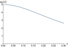
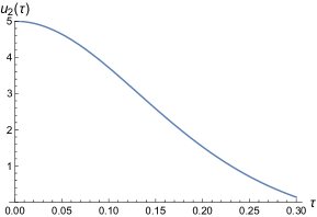
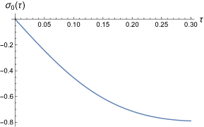
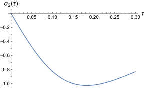
Figure 1: $u_{0}(\tau)$, $u_{2}(\tau)$, $\sigma_{0}(\tau)$, $\sigma_{2}(\tau)$ plotted as functions of $\tau$ for $\tilde{\alpha}=0.1$, $\kappa=5/4$, $\bar{u}_{0}=\bar{u}_{2}=5$ and $\bar{\sigma}_{0}=\bar{\sigma}_{2}=0$.

Let us consider a state with a three-dimensional local structure with $T^{3}$ topology, the translational and space inversion symmetry. For simplicity, let us consider $L=\ell^{3}$ for an integer $\ell$. The natural mapping from sites to $T^{3}$ is $r_{i}=\left(i\mod\ell,~{}~{}\lfloor\frac{i}{\ell}\rfloor\mod\ell,~{}~{}\lfloor\frac{i}{\ell^{2}}\rfloor\mod\ell\right)$ for $1\leq i\leq L$, where $\lfloor x\rfloor$ is the floor function. In $T^{3}$, the periodic boundary condition is used with $(x,y,z)\sim(x+\ell,y,z)\sim(x,y+\ell,z)\sim(x,y,z+\ell)$. In the Fourier space, the collective variables satisfy

$$\frac{\partial U_{k}}{\partial\tau}=4{\cal s}_{k}U_{k},~{}~{}~{}~{}\frac{\partial{\cal s}_{k}}{\partial\tau}=-2\tilde{\alpha}U_{k}^{2}+2{\cal s}_{k}^{2},$$ (32)

where $k=\frac{2\pi}{\ell}(n_{1},n_{2},n_{3})$ with $-\ell/2\leq n_{i}<\ell/2$ denotes three-dimensional momenta, $U_{k}=\sum_{j}e^{-ikr_{j}}~{}U_{r_{j},0}$ and ${\cal s}_{k}=\sum_{j}e^{-ikr_{j}}~{}{\cal s}^{r_{j},0}$. The solution of Eq. (31) is given by

$$U_{k}(\tau)=\frac{U_{k}(0)}{(1-2{\cal s}_{k}(0)\tau)^{2}+4\tilde{\alpha}U_{k}(0)^{2}\tau^{2}},~{}~{}~{}{\cal s}_{k}(\tau)=\frac{{\cal s}_{k}(0)-2\left[{\cal s}_{k}(0)^{2}+\tilde{\alpha}U_{k}(0)^{2}\right]\tau}{(1-2{\cal s}_{k}(0)\tau)^{2}+4\tilde{\alpha}U_{k}(0)^{2}\tau^{2}}.$$ (33)

For states with local structures, $U_{k}$ and ${\cal s}_{k}$ are analytic functions of $k$ and can be expanded around $k=0$ as

$$U_{k}(\tau)=u_{0}(\tau)+u_{2}(\tau)k^{2}+O(k^{4}),~{}~{}~{}{\cal s}_{k}(\tau)=\sigma_{0}(\tau)+\sigma_{2}(\tau)k^{2}+O(k^{4}),$$ (34)

where $k^{2}\equiv\sum_{\mu=1}^{3}(k_{\mu})^{2}$. While $U_{k}$ and ${\cal s}_{k}$ have only the discrete rotational symmetry at the lattice scale, at small $k$ the full rotational symmetry emerges. The coefficients of $U_{k}$ and ${\cal s}_{k}$ evolve as

$$u_{0}(\tau)=\frac{\bar{u}_{0}}{(1-2\bar{\sigma}_{0}\tau)^{2}+4\tilde{\alpha}\bar{u}_{0}^{2}\tau^{2}},~{}~{}u_{2}(\tau)=\frac{\bar{u}_{2}-4\tau\left[\bar{u}_{2}\left(\bar{\sigma}_{0}-\bar{\sigma}_{0}^{2}\tau+\tilde{\alpha}\tau\bar{u}_{0}^{2}\right)+\bar{\sigma}_{2}\bar{u}_{0}(2\bar{\sigma}_{0}\tau-1)\right]}{\left[(1-2\bar{\sigma}_{0}\tau)^{2}+4\tilde{\alpha}\bar{u}_{0}^{2}\tau^{2}\right]^{2}},$$

$$\sigma_{0}(\tau)=\frac{-2\bar{\sigma}_{0}^{2}\tau+\bar{\sigma}_{0}-2\tilde{\alpha}\bar{u}_{0}^{2}\tau}{(1-2\bar{\sigma}_{0}\tau)^{2}+4\tilde{\alpha}\bar{u}_{0}^{2}\tau^{2}},~{}~{}\sigma_{2}(\tau)=\frac{\bar{\sigma}_{2}(1-2\bar{\sigma}_{0}\tau)^{2}-4\tilde{\alpha}\bar{u}_{0}(-2\bar{\sigma}_{0}\bar{u}_{2}\tau+\bar{\sigma}_{2}\bar{u}_{0}\tau+\bar{u}_{2})\tau}{\left[(1-2\bar{\sigma}_{0}\tau)^{2}+4\tilde{\alpha}\bar{u}_{0}^{2}\tau^{2}\right]^{2}},$$

where $\bar{u}_{0}=u_{0}(0)$, $\bar{u}_{2}=u_{2}(0)$, $\bar{\cal s}_{0}={\cal s}_{0}(0)$ and $\bar{\cal s}_{2}={\cal s}_{2}(0)$. These functions are plotted in Fig. 1 for a choice of initial condition.

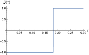
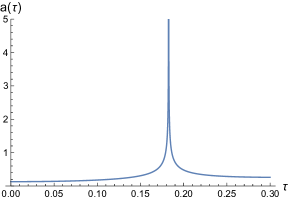
Figure 2: The signature and the scale factor plotted as functions of $\tau$ for the same parameters used in Fig. 1. Initially, the de Sitter-like spacetime with the Lorentzian signature is realized, where the scale factor increases with increasing parameter time. The spacetime undergoes a phase transition into a Euclidean spacetime around $\tau_{c}=0.182$. The signature-changing phase transition is accompanied with the divergent scale factorLee (2020).

The signature and the spatial metric is determined from Eq. (26), which reduces to

$$-{\cal S}g^{\mu\nu}(r)=\left.-6\sum_{m,n}\left[\tilde{\alpha}U^{2}-{\cal s}^{2}\right]^{nm}r^{\mu}_{nm}r^{\nu}_{nm}\right|_{\frac{r_{n}+r_{m}}{2}=r}.$$ (36)

Because the spatial metric gives the uniform and flat three torus with a time dependent scale factor, we obtain the Friedmann–Robertson–Walker (FRW) metricLee (2020),

$$ds^{2}={\cal S}(\tau)d\tau^{2}+a(\tau)^{2}dx^{\mu}dx^{\mu},$$ (37)

where ${\cal S}(\tau)$ is the signature of time and $a(\tau)$ is the scale factor of the uniform space given by

$${\cal S}(\tau) = -\mbox{sgn}\left(\left[\tilde{\alpha}u_{0}(\tau)u_{2}(\tau)-\sigma_{0}(\tau)\sigma_{2}(\tau)\right]\right),$$

$$a(\tau) = \frac{1}{\sqrt{24|\tilde{\alpha}u_{0}(\tau)u_{2}(\tau)-\sigma_{0}(\tau)\sigma_{2}(\tau)|}}.$$ (38)

The signature and scale factor associated with the solution shown in Fig. 1 are plotted in Fig. 2. The saddle point solution determines the background spacetime. In the following, we examine the dynamics of the spin-$2$ mode that propagates on this spacetime. At a critical parameter time $\tau_{c}\approx 0.182$, there is a phase transition at which the scale factor diverges and the signature of spacetime jumps. Signature-changing transitions have been also studied in Ref. Bojowald and Brahma (2017); Stern and Xu (2018). Here we will focus on the range of parameter time ($0<\tau<\tau_{c}$) in which the spacetime is Lorentzian (${\cal S}=-1$) and the space is expanding.

V Graviton

Small fluctuations of the collective variables above the translationally invariant solution are described by the linearized equations,

$$\frac{\partial\delta U_{k_{1}k_{2}}}{\partial\tau} = 2({\cal s}_{k_{1}}+{\cal s}_{k_{2}})\delta U_{k_{1}k_{2}}+2(U_{k_{1}}+U_{k_{2}})\delta{\cal s}_{k_{1}k_{2}},$$

$$\frac{\partial\delta{\cal s}_{k_{1}k_{2}}}{\partial\tau} = -2\tilde{\alpha}(U_{k_{1}}+U_{k_{2}})\delta U_{k_{1}k_{2}}+2({\cal s}_{k_{1}}+{\cal s}_{k_{2}})\delta{\cal s}_{k_{1}k_{2}},$$ (39)

where $\delta U_{k_{1}k_{2}}=\sum_{r_{1}r_{2}}e^{-ik_{1}r_{1}-ik_{2}r_{2}}~{}\delta U_{r_{1},r_{2}}$ and $\delta{\cal s}_{k_{1}k_{2}}=\sum_{r_{1}r_{2}}e^{-ik_{1}r_{1}-ik_{2}r_{2}}~{}\delta{\cal s}^{r_{1},r_{2}}$. A deviation of $g^{\mu\nu}$ denoted as $h^{\mu\nu}$ is linearly related to $\delta U$ and $\delta{\cal s}$. In the Fourier space, the metric fluctuation with momentum $k$ is written as

$$h^{\mu\nu}_{k} = -6{\cal S}\Biggl{\{}\Delta^{\mu\nu}\Bigl{[}\tilde{\alpha}(U_{k_{1}}+U_{k_{2}})\delta U_{k_{1}k_{2}}-({\cal s}_{k_{1}}+{\cal s}_{k_{2}})\delta{\cal s}_{k_{1}k_{2}}\Bigr{]}\Biggr{\}}_{k_{1}=k_{2}=\frac{k}{2}},$$ (40)

where $\Delta^{\mu\nu}\equiv\left(\frac{\partial}{\partial k_{1\mu}}-\frac{\partial}{\partial k_{2\mu}}\right)\left(\frac{\partial}{\partial k_{1\nu}}-\frac{\partial}{\partial k_{2\nu}}\right)$. A traceless transverse mode can be isolated as $h_{k}\equiv a^{2}\epsilon_{\mu\nu}h^{\mu\nu}_{k}$, where $\epsilon_{\mu\nu}$ is a time-independent polarization tensor that satisfies $\epsilon_{\mu\nu}k^{\nu}=0$ and $\epsilon^{\mu}_{~{}\mu}=0$. Due to $\epsilon_{\mu\nu}\frac{\partial}{\partial k_{\mu}}U_{k}=\epsilon_{\mu\nu}\frac{\partial^{2}}{\partial k_{\mu}\partial k_{\nu}}U_{k}=0$, which is guaranteed by the inversion symmetry and the discrete rotational symmetry of the background configuration, the traceless transverse mode is given by

$$h_{k}=-12{\cal S}a^{2}\epsilon_{\mu\nu}\Biggl{\{}\tilde{\alpha}U_{k/2}\Delta^{\mu\nu}\delta U_{k_{1}k_{2}}-{\cal s}_{k/2}\Delta^{\mu\nu}\delta{\cal s}_{k_{1}k_{2}}\Biggr{\}}_{k_{1}=k_{2}=\frac{k}{2}}.$$ (41)

The equation of motion of $h_{k}$ directly follows from Eq. (39). To the second order in $k$ and the number of derivatives in time, it becomes

$$\ddot{h}_{k}+\left[\frac{15u_{0}\dot{u_{2}}-u_{2}\dot{u_{0}}}{4u_{0}u_{2}}\right]\dot{h}_{k}-{\cal S}k^{2}h_{k}=0.$$ (42)

Here, $\dot{f}\equiv\partial_{\eta}f$ and $\ddot{f}\equiv\partial_{\eta}^{2}f$, where $\eta$ is the conformal time defined from $d\eta=a(\tau)^{-1}d\tau$. Eq. (42) describes a massless spin-$2$ mode propagating in the presence of time dependent background metric and other fieldsLifshitz (2017). In the Lorentzian spacetime (${\cal S}=-1$), the low-energy graviton propagates with speed $1$ in the background metric given by Eqs. (37) and (38). This indicates that the local Lorentz invariance emerges in the frame that supports local clocks. The uniqueness of general relativity as a Lorentz-invariant interacting theory of gapless spin-$2$ particleWeinberg (1995) suggests that the present theory includes general relativity as an effective theory for states with local structures in a gauge that supports an extended space and local clocks.

VI Toward an isolated graviton

One way to understand why the gapless graviton is present as a propagating mode is to view the theory for the collective variables in Eq. (8) as the holographic dual of a boundary theory. In this perspective, the exponent of the wavefunction in Eq. (6) is identified as the action of a non-unitary boundary theory, and the Hamiltonian constraint becomes the generator of the evolution along the emergent radial directionLee (2014, 2016). As is the case for the AdS/CFT correspondencerMaldacena (1999); Witten (1998); Gubser et al. (1998), every global symmetry of the boundary theory is promoted to a gauge symmetry in the bulk, and an unbroken symmetry in the boundary gives rise to a gapless gauge field in the bulkNakayama (2013); Bednik (2014). In the present theory, the gauge symmetry includes the space diffeomorphism generated by the momentum constraint. Therefore, the unbroken translational symmetry in Eq. (6) gives rise to a gapless gauge field associated with it, which is the gapless graviton.

Besides the gapless graviton, there also exists a continuum of spin-$2$ modes in the present model. Those modes are labeled by the relative momentum of bi-local fields,

$$h^{\mu\nu}_{k,q} = -6{\cal S}\Biggl{\{}\Delta^{\mu\nu}\Bigl{[}\tilde{\alpha}(U_{k_{1}}+U_{k_{2}})\delta U_{k_{1}k_{2}}-({\cal s}_{k_{1}}+{\cal s}_{k_{2}})\delta{\cal s}_{k_{1}k_{2}}\Bigr{]}\Biggr{\}}_{k_{1}=\frac{k+q}{2},k_{2}=\frac{k-q}{2}},$$ (43)

where $k$ is the center of mass momentum and $q$ is the relative momentum of $\delta U_{k1,k2}$. The gapless graviton in Eq. (40) corresponds to the mode with $q=0$. If both $k$ and $q$ are transverse to the polarization ($\epsilon_{\mu\nu}k^{\nu}=\epsilon_{\mu\nu}q^{\nu}=0$), $h_{k,q}\equiv a^{2}\epsilon_{\mu\nu}h^{\mu\nu}_{k,q}$ satisfies the equation of motion similar to Eq. (42),

$$\ddot{h}_{k,q}+\left[\frac{15u_{0}\dot{u_{2}}-u_{2}\dot{u_{0}}}{4u_{0}u_{2}}\right]\dot{h}_{k,q}-{\cal S}(k^{2}+m_{q}^{2})h_{k,q}=0,$$ (44)

where the $q$-dependent mass goes as $m_{q}^{2}=q^{2}$ in the small $q$ limit. The existence of the continuum of modes is a consequence of the fact that both the center of mass momentum and the relative momentum of the bi-local fields are conserved. This feature is shared with the holographic descriptions of vector models in the large $N$ limit Klebanov and Polyakov (2002); Das and Jevicki (2003); Koch et al. (2011); Douglas et al. (2011); Pando Zayas and Peng (2013); Leigh et al. (2014, 2015); Mintun and Polchinski (2014); Vasiliev (1996, 1999); Giombi and Yin (2010); Vasiliev (2003); Maldacena and Zhiboedov (2013a, b); Sachs (2014); Lee (2016). In order to remove this unrealistic feature, one has to allow mixing between modes with different relative momenta. In this section, we discuss how such mixing arises through $1/N$ corrections.

Figure 3: The left diagram shows the cubic vertex for the bi-local field $\delta T_{2}$ shown in Eq. (45). The momentum along each single line is preserved. As a result, the one-loop self-energy, shown in the right, is diagonal both in the center of mass momentum and the relative momentum of the bi-local field.

To consider $1/N$ corrections, we need the full theory in Eq. (8). The theory for the propagating modes can be obtained by expanding the collective fields around the the saddle-point $\{\bar{q},\bar{s},\bar{P}_{1},\bar{T}_{1},\bar{P}_{2},\bar{T}_{2}\}$ and writing down the theory for the fluctuating variables $\{\delta q,\delta s,\delta P_{1},\delta T_{1},\delta P_{2},\delta T_{2}\}$. The quadratic part determines the free propagator, which can be obtained from the equation of motion obeyed by the fluctuating variables. The full theory also include interaction vertices. For example, $\tilde{\alpha}UQU$ in Eq. (8) includes a cubic vertex for $\delta T_{2}$, $4\tilde{\alpha}~{}\mbox{tr}\left\{{\delta T_{2}\bar{P}_{2}\delta T_{2}\bar{P}_{2}\delta T_{2}}\right\}$ for the choice of $v=I$. In the Fourier space, the vertex can be written as

$$4\tilde{\alpha}\int dk_{1}dk_{2}dk_{3}~{}V_{k_{1},k_{2},k_{3}}~{}\delta T_{2}^{k_{1},-k_{2}}\delta T_{2}^{k_{2},-k_{3}}\delta T_{2}^{k_{3},-k_{1}},$$ (45)

where $V_{k_{1},k_{2},k_{3}}=\bar{P}_{2;k_{2},-k_{2}}\bar{P}_{2;k_{3},-k_{3}}$. At the saddle-point, the collective fields have non-zero expectation values only for the modes with zero center of mass momentum due to the translational invariance. In general, loop corrections can modify the quadratic action for $\delta T_{2}$ as

$$\delta S=\int dk_{1}dk_{2}dk_{3}dk_{4}~{}\Sigma_{k_{1},k_{2};k_{3},k_{4}}\left(\delta T_{2}^{k1,k2}\right)^{*}\delta T_{2}^{k3,k4},$$ (46)

where $\Sigma_{k_{1},k_{2};k_{3},k_{4}}$ denotes the self-energy of $\delta T_{2}$, which is suppressed by $1/N$ compared to Eq. (8). The self-energy generated from Eq. (45) through the one-loop diagram in Fig. 3 takes the form of

$$\Sigma_{k_{1},k_{2};k_{3},k_{4}}\sim\left(\delta_{k_{1},k_{3}}\delta_{k_{2},k_{4}}+\delta_{k_{1},k_{4}}\delta_{k_{2},k_{3}}\right)\int dqV_{k_{1},-k_{2},-q}V_{-k_{1},q,k_{2}}G_{2}(-k_{1},-q)G_{2}(q,-k_{2}),$$ (47)

where $G_{2}(k_{1},k_{2})$ is the propagator of $\delta T_{2}^{k_{1},k_{2}}$. It is noted that the self-energy is still diagonal both in the center of mass momentum and the relative momentum. It can be easily checked that no interaction in Eq. (8) gives rise to a mixing between modes with different relative momenta except for the modes with strictly zero center of mass momentum. This is because the vertex in Eq. (45) and all other vertices in Eq. (8) are invariant under $k$-dependent $U(1)$ tranformations, $\delta T_{2}^{k_{1},k_{2}}\rightarrow\delta T_{2}^{k_{1},k_{2}}e^{i(\varphi_{k_{1}}+\varphi_{k_{2}})}$, where $\varphi_{k}$ is $k$-dependent phase angle with $\varphi_{-k}=-\varphi_{k}$. These $U(1)$ symmetries forbid mixing between modes with different relative momenta.

Figure 4: With the lower flavour symmetry group of $O(N/2)\times O(\sqrt{N/2})\times O(\sqrt{N/2})$, additional operators are allowed in the basis states that span the kinematic Hilbert space. Besides the bi-local operators included in Eq. (6), one has to include $W^{C}=\left(\frac{N}{2}\right)^{-\frac{n-1}{2}}~{}\mbox{tr}\left\{{\pi^{i_{1}}(\pi^{i_{2}})^{T}\pi^{i_{3}}(\pi^{i_{4}})^{T}...\pi^{i_{2n-1}}(\pi^{i_{2n}})^{T}}\right\}$ defined on a series of sites $C=(i_{1},i_{2},....,i_{2n})$ that can be viewed as a loop, where $\pi^{i}$ is is the matrix obtained by rearranging $N/2$ components of $\Pi_{A}^{~{}i}$ with $A=L+N/2+1,..,L+N$ into a $\sqrt{N/2}$ by $\sqrt{N/2}$ matrix. In the figure, circles (squares) denote sites with $\pi$ ($\pi^{T}$).

In order to generate mixing between modes with different relative momenta, one has to break these $U(1)$ symmetries. One simple way of achieving this is to enlarge the kinematic Hilbert space from Eq. (6) to the one in which the $O(N/2)\times O(N/2)$ flavour symmetry is further broken down to $O(N/2)\times O(\sqrt{N/2})\times O(\sqrt{N/2})$. The first $O(N/2)$ acts on $\Pi_{A}^{~{}i}$ with $A=L+1,..,L+N/2$ as before. The remaining $O(\sqrt{N/2})\times O(\sqrt{N/2})$ acts on $\Pi_{A}^{~{}i}$ with $A=L+N/2+1,..,M$ as left and right $O(\sqrt{N/2})$ multiplications as $\Pi_{A}^{~{}i}$ is viewed as a matrix. Namely, we identify $N/2$ components of $\Pi_{A}^{~{}i}$ with $A=L+N/2+1,..,M$ as a $\sqrt{N/2}\times\sqrt{N/2}$ matrix : $\Pi_{A}^{~{}i}=\pi_{{\bf a}{\bf b}}^{~{}i}$ with ${\bf a}=\lfloor\frac{A-(L+N/2+1)}{\sqrt{N/2}}+1\rfloor$ and ${\bf b}=\left[A-(L+N/2+1)\mod\sqrt{N/2}\right]+1$ for $A=L+N/2+1,..,M$. Under $O(\sqrt{N/2})\times O(\sqrt{N/2})$, $\pi^{~{}i}$ is transformed as $\pi^{i}\rightarrow o_{L}\pi^{i}o_{R}$, where $o_{L}$ and $o_{R}$ are $\sqrt{N/2}\times\sqrt{N/2}$ orthogonal matrices. The enlarged sub-Hilbert space with the lower flavour symmetry is spanned by a larger set of basis states given by

$$\big{|}q,P_{1},P_{2},X\big{>} = \int D\Pi~{}e^{-i\left[\sqrt{N}\sum_{a=1}^{L}\Pi^{i}_{~{}a}q^{a}_{~{}i}+\sum_{b=L+1}^{L+\frac{N}{2}}P_{1,ij}\Pi_{b}^{~{}i}\Pi_{b}^{~{}j}+P_{2,ij}~{}\mbox{tr}\left\{{\pi^{~{}i}(\pi^{~{}j})^{T}}\right\}\right]}\times$$ (48)

$$~{}~{}~{}~{}~{}e^{-i\sum_{C}X_{C}W^{C}}\big{|}\Pi\big{>}.$$

The first line of Eq. (48) is exactly the same as Eq. (6) because $~{}\mbox{tr}\left\{{\pi^{~{}i}(\pi^{~{}j})^{T}}\right\}=\sum_{b=L+N/2+1}^{M}\Pi_{b}^{~{}i}\Pi_{b}^{~{}j}$. $q$ is an $L\times L$ matrix and $P_{1}$ and $P_{2}$ are $L\times L$ symmetric matrices as before. The second line includes additional operators that are allowed due to the lowered flavour symmetry. Besides what is already included in the first line, the most general operators needed to span the Hilbert space with $O(\sqrt{N/2})\times O(\sqrt{N/2})$ symmetry are the Wilson-loop-like operators $W^{C}=\left(\frac{N}{2}\right)^{-\frac{n-1}{2}}~{}\mbox{tr}\left\{{\pi^{i_{1}}(\pi^{i_{2}})^{T}\pi^{i_{3}}(\pi^{i_{4}})^{T}...\pi^{i_{2n-1}}(\pi^{i_{2n}})^{T}}\right\}$ defined on a series of sites $C=(i_{1},i_{2},....,i_{2n})$ (see Fig. 4)Ma and Lee (2022), where the prefactor normalizes the multi-site loop operators as $W^{C}\sim O(N)$ in the large $N$ limit. In the new term, we only include loop operators with $n\geq 2$ because the bi-local operators, which are the special case of $W^{C}$ with $n=1$, are already included in the first line. The enlarged kinematic Hilbert space is spanned by the bi-local fields and the new multi-local fields $X_{C}$ which are defined in the space of loops.

Figure 5: The dynamics that $Q_{ij}$ induces on loop operators. (a) At the linear order in the source of loop ($X_{C}$), a loop either splits into two loops or shrinks to a smaller loop. If $\pi$ and $\pi^{T}$ are contracted, one loop is broken into two loops. If two $\pi$’s (or two $\pi^{T}$’s) are contracted, one of the segment is reversed before glued to the other segment to form one smaller loop. (b) At the quadratic order in the source, two loops merge into one loop. If $\pi$ and $\pi^{T}$ are contracted, two loops merge without changing their orientations. If two $\pi$’s (or two $\pi^{T}$’s) are contracted, one of the segment is reversed before merging.

Because $\{\big{|}q,P_{1},P_{2},X\big{>}\}$ forms a complete basis of the Hilbert space with the symmetry, $e^{-i\epsilon(\hat{H}_{v_{0}}+\hat{G}_{y_{0}})}\big{|}q,P_{1},P_{2},X\big{>}$ can be expressed as a linear superposition of $\big{|}q,P_{1},P_{2},X\big{>}$. The theory of the new set of collective variables can be derived in the same way that Eq. (8) is derived,

$$S = N\int d\tau~{}\Bigl{[}~{}\mbox{tr}\left\{{s\partial_{\tau}q+T_{1}\partial_{\tau}P_{1}+T_{2}\partial_{\tau}P_{2}}\right\}+\sum_{C}Y^{C}\partial_{\tau}X_{C}$$ (49)

$$-~{}\mbox{tr}\left\{{{\cal H}[q,s,P_{1},T_{1},P_{2},T_{2},X,Y]v+{\cal G}[q,s,P_{1},T_{1},P_{2},T_{2},X,Y]y}\right\}\Bigr{]}.$$

Here $X_{C}$ is the dynamical source for the loop operator just as $P_{1}$ and $P_{2}$ are promoted to dynamical variables in Eq. (8). $Y^{C}$ is the conjugate momentum of $X_{C}$ whose saddle-point value represents the expectation value of the loop operators, $\big{<}Y^{C}\big{>}=\frac{1}{N}\big{<}W^{C}\big{>}$. The momentum constraint and Hamiltonian constraints are modified to

$${\cal G}^{j}_{~{}i}[q,s,P_{1},T_{1},P_{2},T_{2},X_{C},Y^{C}] = \left[sq+2(T_{1}P_{1}+T_{2}P_{2})+i\beta I\right]^{j}_{~{}i}+\sum_{C}Y^{C-i+j}X_{C},$$

$${\cal H}[q,s,P_{1},T_{1},P_{2},T_{2}] = -U+\tilde{\alpha}UQU.$$ (50)

The last term in the momentum constraint is the new addition that describes the action of a generalized diffeomorphism under which loop $C$ is deformed into a new loop $C-i+j$ which is obtained by removing site $i$ with $j$ in $C$. If $C$ does not include $i$, $Y^{C-i+j}=0$. In the Hamiltonian, $U^{ij}=\left(ss^{T}+T_{1}+T_{2}\right)^{ij}$ is unchanged, but $Q_{ij}$ is modified with additional terms that involve general loop fields,

$$Q_{ij} = \left(q^{T}q+\sum_{c}[4P_{c}T_{c}P_{c}+iP_{c}]+2i\sum_{C}X_{C}\sum_{C_{1},C_{2}}F^{C}_{C_{1},C_{2};ij}Y^{C_{1}}Y^{C_{2}}\right.$$ (51)

$$\left.+2\sum_{C}X_{C}\sum_{l}\left[G^{C}_{i}P_{2,jl}Y^{C-i+l}+G^{C}_{j}P_{2,il}Y^{C-j+l}\right]+\sum_{C_{1},C_{2}}X_{C_{1}}X_{C_{2}}G^{C_{1},C_{2}}_{C;ij}Y^{C}\right)_{ij}.$$

Here, the first two terms are the same as before. The third term describes the process where loop $C$ breaks into loops $C_{1}$ and $C_{2}$ with the removal of sites $i$ and $j$ out of $C$ and rejoining the remaining segments. The way the remaining segments are rejoined depends on whether $i$ and $j$ are separated by an even or odd number of sites. If $C$ includes both $i$ and $j$, it can be written as $C=i+C^{\prime}+j+C^{\prime\prime}$ without loss or generality, where $C^{\prime},C^{\prime\prime}$ represent open chains that form loop $C$ once $C^{\prime}$ and $C^{\prime\prime}$ are glued via $i$ and $j$. Let $n_{C^{\prime}}$ denote the number of sites in chain $C^{\prime}$. If $n_{C^{\prime}}$ is even, $F^{C}_{C_{1},C_{2};ij}=1$ for $C_{1}=C^{\prime}$ and $C_{2}=C^{\prime\prime}$. If $n_{C^{\prime}}$ is odd, $F^{C}_{C_{1},C_{2};ij}=\sqrt{2/N}$ for $C_{1}=C^{\prime}+\bar{C}^{\prime\prime}$ and $C_{2}=\emptyset$. Here, $\bar{C}^{\prime\prime}$ denotes the chain constructed by reversing the order of sites in $C^{\prime\prime}$. For the loop made of the empty set, we use the convention of $Y^{\emptyset}\equiv 1/2$. This is illustrated in Fig. 5. While $n_{C}\geq 4$, $n_{C_{1}}$ and $n_{C_{2}}$ can be any non-negative even integer because loops generated from $C$ can be of smaller sizes. For example, $C_{2}=\emptyset$ if $i$ and $j$ are adjacent in $C$. If $C_{2}$ is bi-local with $C_{2}=(ij)$, $Y^{C_{2}}\equiv T_{2}^{ij}$. If $C$ does not include $i$ or $j$, $F^{C}_{C_{1},C_{2};ij}=0$. The fourth term describes the process where loop $C$ merge with a bi-local field $P_{2}$ to create a new loop by replacing site $i$ from $C$ and site $j$ from $P_{2}$, or vice versa. If $C$ includes site $i$, $G^{C}_{i}=1$. Otherwise, $G^{C}_{i}=0$. $C-i+l$ represent the loop obtained by replacing site $i$ with $l$ in $C$. In the last term, loops $C_{1}$ and $C_{2}$ merge into a new loop $C$ by removing a site from each loop and rejoining them. If $C_{1}$ and $C_{2}$ include site $i$ and $j$, respectively, we can write $C_{1}=i+C_{1}^{\prime}$ and $C_{2}=j+C_{2}^{\prime}$. If site $i$ has $\pi$ and $j$ has $\pi^{T}$ (or vice versa), $G^{C_{1},C_{2}}_{C;ij}=1$ for $C=C_{1}^{\prime}+C_{2}^{\prime}$. If site $i$ and $j$ both have $\pi$ (or $\pi^{T}$), $G^{C_{1},C_{2}}_{C;ij}=1$ for $C=C_{1}^{\prime}+\bar{C}_{2}^{\prime}$. This is illustrated in Fig. 5. The induced dynamics of loops is similar to the dynamics that loop fields obey in holographic duals of lattice gauge theoriesLee (2012). It is noted that the second to the last term can be viewed as a special case of the last term where one of the merged loops is just bi-local.

Figure 6: The diagram on the left shows a new cubic vertex for the bi-local field $\delta T_{2}$ in the presence of a non-zero expectation value of the four-site loop field $\bar{X}_{k1,k2,k3,k4}$ as is shown in Eq. (52). Unlike the vertex in , the momentum in each single line does not have to be conserved because the four-site loop field breaks the local $Z_{2}$ symmetry. Consequently, the one-loop self-energy shown in the right panel has a non-zero off-diagonal element between bi-local fields with different relative momenta (see Eq. (53)).

The semi-classical equation of motion for $U$ and ${\cal s}$, which determine the metric, remains the same as Eq. (31) even in the presence of the additional loop fields. This is because $U$ depends only on the bi-local fields $(ss^{T})$, $T_{1}$ and $T_{2}$. Therefore, the equation of motion for the spin-$2$ modes remains the same and there still exist a continuum of spin-$2$ modes labeled by the relative momentum of the bi-local fields in the large $N$ limit. However, differences arise from $1/N$ corrections because the general loop-fields give rise to new interaction vertices. For example, $\tilde{\alpha}UQU$ in Eq. (9) generates a cubic vertex for $\delta T_{2}$, $i\alpha\sum_{ijkl}\delta T_{2}^{ij}\bar{X}_{jklm}\delta T_{2}^{ki}\delta T_{2}^{lm}$, where $\bar{X}_{i_{1}i_{2}i_{3}i_{4}}$ represents the saddle-point value of the four-site loop field. In momentum space, this gives rise to a vertex that breaks the $k$-dependent $U(1)$ symmetry,

$$i\tilde{\alpha}\int dk_{1}dk_{2}dk_{3}dk_{4}~{}\bar{X}_{-k_{1},-k_{3},k_{1}-k_{4},k_{3}+k_{4}}~{}\delta T_{2}^{k_{1},k_{2}}\delta T_{2}^{-k_{2},k_{3}}\delta T_{2}^{-k_{1}+k_{4},-k_{3}-k_{4}}.$$ (52)

Without the $k$-dependent $U(1)$ symmetry, loop-corrections can give rise to the self-energy that is off-diagonal in the space of relative momentum. Through the one-loop correction shown in Fig. 6, one obtains the self-energy for $\delta T_{2}$,

$$\Sigma_{k_{1},k_{2};k_{1}-l,k_{2}+l}\sim\tilde{\alpha}^{2}\int dq~{}\bar{X}_{-k_{1},-q,q,k_{1}}\bar{X}_{-k_{1},-k_{2},k_{1}-l,k_{2}+l}G_{2}(k_{1},q)G_{2}(q,-k_{2}).$$ (53)

While the center of mass momentum is still conserved, the self-energy mixes modes with different relative momenta. This off-diagonal self-energy also creates mixing between $\delta U_{\frac{k+q}{2},\frac{k-q}{2}}$ and $\delta U_{\frac{k+q^{\prime}}{2},\frac{k-q^{\prime}}{2}}$ for $q\neq q^{\prime}$ because $\delta T_{2}$ linearly mixes with $\delta U$. In the presence of such mixings, the eigenmodes of the wave equation derived from the quantum effective action should be given by linear superpositions of modes with different relative momenta as

$$\delta U^{(l)}_{k}=\int dq~{}f^{(l)}_{k,q}\delta U_{\frac{k+q}{2},\frac{k-q}{2}},$$ (54)

where each eigenmode is labeled by the center of mass momentum $k$ and an additional label $l$. Finding the eigenvector $f^{(l)}_{k,q}$ reduces to the problem of diagonalizing a quantum mechanical Hamiltonian of a ‘particle’ moving in the space of relative momentum. The particle is subject to a potential $Nm_{q}^{2}$ because of the mass term that is diagonal in relative momentum (see Eq. (44)). The off-diagonal self-energy allows the particle to hop from $q$ to $q^{\prime}$ with hopping amplitude proportional to $\Sigma_{\frac{k+q}{2},\frac{k-q}{2};\frac{k+q^{\prime}}{2},\frac{k-q^{\prime}}{2}}$. The diagonalization of the Hamiltonian will give rise to a discrete set of bound states at low energies because the $Nm_{q}^{2}$ provides a harmonic potential at low $q$. The true graviton should stay gapless due to the diffeomorphism invariance and the unbroken translational invariance. However, other spin-$2$ modes are expected to acquire non-zero masses that are order of $1/N$ as their masses are not protected from quantum corrections.

VII Discussion

In this paper, we show that the model of quantum gravity proposed in Ref. Lee (2020) supports a gapless spin-$2$ excitation as a propagating mode. Although the model has no pre-determined partitioning of the Hilbert space into local Hilbert spaces, the low-energy effective theory takes the form of a local theory with an emergent Lorentz symmetry in a frame where the pattern of entanglement exhibits a local structure and local clocks are well defined. We conclude with some open questions. First, the present model has a continuum of spin-$2$ modes with a continuously varying mass in the large $N$ limit. This unrealistic feature is expected to go away once the kinematic Hilbert space is enlarged and $1/N$ corrections are included as is discussed in the previous section. It will be of interest to take into account all leading $1/N$ corrections and compute the full mass spectrum of the propagating modes. However, this wouldn’t be fully satisfactory in that there are still light massive spin-$2$ modes in the semi-classical limit. It is desirable to find a new mechanism that isolates the massless graviton from other massive modes with a mass gap that is not suppressed in the large $N$ limit. Second, the present theory suffers from the cosmological constant problem. Without fine tuning, there is no separation between the scale that controls the rate at which time dependent background fields change and the scale that suppresses higher derivative terms in the effective theory. It would be interesting to consider an alternative model (possibly a supersymmetric model) that stabilizes the flat spacetime as a saddle point. Despite these drawbacks, this model serves as a concrete toy model of quantum gravity that realizes some interesting features that the true theory of quantum gravity may share. Those features are the Hilbert-space-partition-independence and the emergence of dimension, topology, signature and geometry of spacetime. Finally, we comment on the relation between the present model and the BFSS/IKKT matrix models that have been proposed as a non-perturbative formulation of string theoryBanks et al. (1997); Ishibashi et al. (1997); Brahma et al. (2023). Those matrix models share the same goal of realizing emergent spacetime from non-geometric microscopic degrees of freedom. However, one notable difference is the fact that the number of non-compact spacetime directions is bounded by the number of matrices in the previous matrix models. In the present model, the spacetime dimension is dynamical, and there are states that exhibit spacetimes with any dimension. It would be interesting to know if there is any relation between the earlier matrix models and the present model restricted to a sub-Hilbert space with a fixed spacetime dimension. Ultimately, it will be great to understand a dynamical mechanism that selects certain spacetime dimensions in the model where the spacetime dimension is fully dynamical.

References

- Maldacena (1999) J. M. Maldacena, Int.J.Theor.Phys. 38, 1113 (1999), eprint hep-th/9711200.
- Witten (1998) E. Witten, Adv.Theor.Math.Phys. 2, 253 (1998), eprint hep-th/9802150.
- Gubser et al. (1998) S. Gubser, I. R. Klebanov, and A. M. Polyakov, Phys.Lett. B428, 105 (1998), eprint hep-th/9802109.
- Ryu and Takayanagi (2006) S. Ryu and T. Takayanagi, Phys. Rev. Lett. 96, 181602 (2006), URL http://link.aps.org/doi/10.1103/PhysRevLett.96.181602.
- Klebanov and Polyakov (2002) I. R. Klebanov and A. M. Polyakov, Physics Letters B 550, 213 (2002), eprint hep-th/0210114.
- Hubeny et al. (2007) V. E. Hubeny, M. Rangamani, and T. Takayanagi, Journal of High Energy Physics 2007, 062 (2007), URL http://stacks.iop.org/1126-6708/2007/i=07/a=062.
- Van Raamsdonk (2010) M. Van Raamsdonk, Gen. Rel. Grav. 42, 2323 (2010), [Int. J. Mod. Phys.D19,2429(2010)], eprint 1005.3035.
- Lewkowycz and Maldacena (2013) A. Lewkowycz and J. Maldacena, Journal of High Energy Physics 2013, 1 (2013), ISSN 1029-8479, URL http://dx.doi.org/10.1007/JHEP08(2013)090.
- Kiritsis (2013) E. Kiritsis, Journal of High Energy Physics 1, 30 (2013), eprint 1207.2325.
- Headrick et al. (2014) M. Headrick, V. E. Hubeny, A. Lawrence, and M. Rangamani, Journal of High Energy Physics 2014, 162 (2014), URL https://doi.org/10.1007/JHEP12(2014)162.
- Faulkner et al. (2013) T. Faulkner, A. Lewkowycz, and J. Maldacena, Journal of High Energy Physics 2013, 74 (2013), URL https://doi.org/10.1007/JHEP11(2013)074.
- Lashkari et al. (2014) N. Lashkari, M. B. McDermott, and M. Van Raamsdonk, Journal of High Energy Physics 2014, 195 (2014), URL https://doi.org/10.1007/JHEP04(2014)195.
- Anninos et al. (2017) D. Anninos, T. Hartman, and A. Strominger, Classical and Quantum Gravity 34, 015009 (2017).
- Lee (2014) S.-S. Lee, Journal of High Energy Physics 2014, 76 (2014), ISSN 1029-8479, URL https://doi.org/10.1007/JHEP01(2014)076.
- Faulkner et al. (2014) T. Faulkner, M. Guica, T. Hartman, R. C. Myers, and M. Van Raamsdonk, Journal of High Energy Physics 3, 51 (2014), eprint 1312.7856.
- Cao et al. (2017) C. Cao, S. M. Carroll, and S. Michalakis, Phys. Rev. D 95, 024031 (2017), URL https://link.aps.org/doi/10.1103/PhysRevD.95.024031.
- Maldacena and Susskind (2013) J. Maldacena and L. Susskind, Fortschritte der Physik 61, 781 (2013), eprint https://onlinelibrary.wiley.com/doi/pdf/10.1002/prop.201300020, URL https://onlinelibrary.wiley.com/doi/abs/10.1002/prop.201300020.
- Lee (2020) S.-S. Lee, Journal of High Energy Physics 2020, 70 (2020), URL https://doi.org/10.1007/JHEP06(2020)070.
- Lee (2021) S.-S. Lee, Journal of High Energy Physics 2021, 204 (2021), URL https://doi.org/10.1007/JHEP04(2021)204.
- Arnowitt et al. (1959) R. Arnowitt, S. Deser, and C. W. Misner, Phys. Rev. 116, 1322 (1959), URL https://link.aps.org/doi/10.1103/PhysRev.116.1322.
- Teitelboim (1973) C. Teitelboim, Annals of Physics 79, 542 (1973), ISSN 0003-4916, URL http://www.sciencedirect.com/science/article/pii/0003491673900961.
- Bojowald and Brahma (2017) M. Bojowald and S. Brahma, Phys. Rev. D 95, 124014 (2017), URL https://link.aps.org/doi/10.1103/PhysRevD.95.124014.
- Stern and Xu (2018) A. Stern and C. Xu, Phys. Rev. D 98, 086015 (2018), URL https://link.aps.org/doi/10.1103/PhysRevD.98.086015.
- Lifshitz (2017) E. Lifshitz, General Relativity and Gravitation 49, 18 (2017), URL https://doi.org/10.1007/s10714-016-2165-8.
- Weinberg (1995) S. Weinberg, The Quantum Theory of Fields, vol. 1 (Cambridge University Press, 1995).
- Lee (2016) S.-S. Lee, Journal of High Energy Physics 2016, 44 (2016), ISSN 1029-8479, URL https://doi.org/10.1007/JHEP09(2016)044.
- Nakayama (2013) Y. Nakayama, International Journal of Modern Physics A 28, 1350166 (2013), eprint https://doi.org/10.1142/S0217751X13501662, URL https://doi.org/10.1142/S0217751X13501662.
- Bednik (2014) G. Bednik, Master’s thesis, McMaster University, http://hdl.handle.net/11375/15452 (2014).
- Das and Jevicki (2003) S. R. Das and A. Jevicki, Phys.Rev. D68, 044011 (2003), eprint hep-th/0304093.
- Koch et al. (2011) R. d. M. Koch, A. Jevicki, K. Jin, and J. P. Rodrigues, Phys.Rev. D83, 025006 (2011), eprint 1008.0633.
- Douglas et al. (2011) M. R. Douglas, L. Mazzucato, and S. S. Razamat, Phys.Rev. D83, 071701 (2011), eprint 1011.4926.
- Pando Zayas and Peng (2013) L. A. Pando Zayas and C. Peng, ArXiv e-prints (2013), eprint 1303.6641.
- Leigh et al. (2014) R. G. Leigh, O. Parrikar, and A. B. Weiss, Phys.Rev. D89, 106012 (2014), eprint 1402.1430.
- Leigh et al. (2015) R. G. Leigh, O. Parrikar, and A. B. Weiss, Phys. Rev. D 91, 026002 (2015), eprint 1407.4574.
- Mintun and Polchinski (2014) E. Mintun and J. Polchinski, ArXiv e-prints (2014), eprint 1411.3151.
- Vasiliev (1996) M. A. Vasiliev, Int.J.Mod.Phys. D5, 763 (1996), eprint hep-th/9611024.
- Vasiliev (1999) M. A. Vasiliev (1999), eprint hep-th/9910096.
- Giombi and Yin (2010) S. Giombi and X. Yin, JHEP 1009, 115 (2010), eprint 0912.3462.
- Vasiliev (2003) M. Vasiliev, Phys.Lett. B567, 139 (2003), eprint hep-th/0304049.
- Maldacena and Zhiboedov (2013a) J. Maldacena and A. Zhiboedov, J.Phys. A46, 214011 (2013a), eprint 1112.1016.
- Maldacena and Zhiboedov (2013b) J. Maldacena and A. Zhiboedov, Class.Quant.Grav. 30, 104003 (2013b), eprint 1204.3882.
- Sachs (2014) I. Sachs, Phys. Rev. D 90, 085003 (2014), eprint 1306.6654.
- Ma and Lee (2022) H. Ma and S.-S. Lee, SciPost Phys. 12, 046 (2022), URL https://scipost.org/10.21468/SciPostPhys.12.2.046.
- Lee (2012) S.-S. Lee, Nucl.Phys. B862, 781 (2012), eprint 1108.2253.
- Banks et al. (1997) T. Banks, W. Fischler, S. H. Shenker, and L. Susskind, Phys. Rev. D 55, 5112 (1997), URL https://link.aps.org/doi/10.1103/PhysRevD.55.5112.
- Ishibashi et al. (1997) N. Ishibashi, H. Kawai, Y. Kitazawa, and A. Tsuchiya, Nuclear Physics B 498, 467 (1997), ISSN 0550-3213, URL https://www.sciencedirect.com/science/article/pii/S0550321397002903.
- Brahma et al. (2023) S. Brahma, R. Brandenberger, and S. Laliberte, Physics 5, 1 (2023), ISSN 2624-8174, URL https://www.mdpi.com/2624-8174/5/1/1.